1

Work in progress (first draft)

LOW-LEVEL FRACTALITY AND THE TERASCALE SECTOR OF FIELD THEORY

Ervin Goldfain

Advanced Technology and Sensor Group, Welch Allyn Inc., Skaneateles Falls, NY 13153

Abstract

As it is widely known, the Standard Model for particle physics (SM) has been successfully tested at all accelerator

facilities and is currently the best tool available for understanding the phenomena on the subatomic scale.

Conventional wisdom is that the SM represents only the low-energy limit of a more fundamental theory and that it

can be consistently extrapolated to scales many orders of magnitude beyond the energy levels probed by the Large

Hadron Collider (LHC).

Despite its impressive performance, the SM leaves out a fairly large number of unsolved puzzles. In contrast with

the majority of mainstream proposals on how to address these challenges, the approach developed here exploits the

idea that space-time dimensionality becomes scale-dependent near or above the low TeV scale. This conjecture has

recently received considerable attention in theoretical physics and goes under several designations, from

“continuous dimension” to “dimensional flow” and “fractional field theory”. Drawing from the principles of the

Renormalization Group program, our key finding is that the SM represents a self-contained multifractal set. The set

is defined on continuous space-time having arbitrarily small deviations from four-dimensions, referred to as a

“minimal fractal manifold” (MFM). This work explores the full dynamical implications of the MFM and, staying

consistent with experimental data, it offers novel explanations on some of the unsolved puzzles raised by the SM.

2

“Rereading classic theoretical physics textbooks leaves a sense that there are holes large enough to steam a

Eurostar train through them. Here we learn about harmonic oscillators and Keplerian ellipses - but where is the

chapter on chaotic oscillators, the tumbling Hyperion? We have just quantized hydrogen, where is the chapter on

the classical 3-body problem and its implications for quantization of helium? We have learned that an instanton is a

solution of field-theoretic equations of motion, but shouldn’t a strongly nonlinear field theory have turbulent

solutions? How are we to think about systems where things fall apart; the center cannot hold; every trajectory is

unstable?”

“Chaos: Classical and Quantum I: Deterministic Chaos “

- P. Cvitanovic et al.

( http://chaosbook.org/chapters/ChaosBook.pdf )

INTRODUCTION

This study develops a new perspective on the dynamical structure of the Standard Model for

particle physics (SM), a framework that successfully explains the subatomic world and its

fundamental interactions. The SM includes the (3) (2) (1)SU SU U gauge model of strong

and electroweak interactions along with the Higgs mechanism that spontaneously breaks the

electroweak (2) (1)SU U group down to the (1)U group of electrodynamics. It has been

confirmed countless times in all accelerator experiments, including the first round of runs at the

LHC. The main motivation behind this study stems in the fact that, despite being

overwhelmingly supported by experimental data, the SM has many puzzling aspects, such as the

large number of physical parameters, a triplication of chiral families and the existence of three

gauge interactions. Some of the unsettled issues revolve around the following questions:

3

Is the Higgs boson solely responsible for the electroweak symmetry breaking and the

origin of mass? The current view supports this assertion, although understanding of the

Higgs sector remains widely open at this time [ ]. There are two primary mass-generation

mechanisms in the SM: the Higgs mechanism of electroweak symmetry breaking,

accounting for the spectrum of massive gauge bosons and fermions, and dimensional

transmutation, partially responsible for the mass of baryonic matter. While technical

aspects of both mechanisms are well under control, neither one is able to uncover the

origin of the electroweak scale or of the Higgs boson mass.

Are fundamental parameters of the SM finely tuned? The mass of the Higgs boson is

sensitive to the physics at high energy scales. If there is no physics beyond the SM, the

elementary Higgs mass parameter must be adjusted to an accuracy order of 1 part in 1032

in order to explain the large gap between the low TeV scale and the Planck scale [ ].

What is the origin of quark, lepton and neutrino mass hierarchies and mixing angles?

These “flavor” parameters account for most of the basic parameters of the SM, and their

pattern remains elusive. New particles at or above the TeV scale with flavor-dependent

coupling charges are postulated in many scenarios, and observation of such particles

would provide critical insights to these puzzles [ ].

What is the physical nature and composition of Dark Matter and how is the SM related to

the gravitational interaction?

What is the underlying mechanism behind the matter-antimatter asymmetry in the

Universe?

It is generally believed that we are at a crossroads in the development of high-energy theory. Is

there any compelling path to follow in our model-building efforts? We came a long way to

4

recognize that, in general, Nature fails to fit the streamlined framework of conventional quantum

field theories (QFT). Systems of quantum fields that are

weakly interacting,

nearly linear and stable against disturbances,

perturbatively renormalizable,

form the backbone of “effective” QFT and are likely to represent exceptions rather than the rule.

And yet we also know that both QFT and SM work exceptionally well up to the low TeV range

probed by the LHC. A dilemma has undoubtedly surfaced on how to best proceed. For example,

over the years, the many unsolved challenges of the SM led to an overflow of extensions

targeting the physics beyond the SM scale. The majority of these proposals focus on solving

some unsatisfactory aspects of the theory while introducing new unknowns. Experiments are

expected to provide guidance in pointing to the correct theory yet, so far, LHC searches show no

credible hint for physics beyond the SM up to a center-of-mass energy of s = 8 TeV [ ].

These results, albeit entirely preliminary, suggest two possible scenarios, namely:

SM fields are either decoupled or ultra-weakly coupled to new dynamic structures

emerging in the low or intermediate TeV scale,

There is an undiscovered and possibly non-trivial connection between the SM and TeV

phenomena.

It is often said that progress on the theoretical front requires understanding the first principles

that drive Nature. The guiding principle we follow throughout this study is the universal

5

behavior of nonlinear dynamical systems. Our belief is that there are strong reasons to conclude

that this principle underlies a broad range of phenomena on the subatomic scale. In particular,

The universality principle is a natural tool for decoding the dynamics of the SM, a

manifestly nonlinear theory whose structure is based on self-interacting gauge and Higgs

fields. As explained below, the principle also implies that space-time dimensionality

becomes scale-dependent near or above the low TeV scale. This conjecture has recently

seen growing interest in theoretical physics and goes under several designations, from

“continuous dimension” to “dimensional flow” and “fractional field theory”. Drawing

from the ideas of the Renormalization Group (RG) program, a key finding below is that

the SM represents a self-contained multifractal set. The set is defined on continuous

space-time having arbitrarily small deviations from four-dimensions, referred to as a

“minimal fractal manifold” (MFM). Here we explore the dynamical implications of the

MFM and, staying consistent with experimental data, we show that they offer novel

explanations for some of the unsolved puzzles raised by the SM.

In contrast with many mainstream proposals, the universality principle hints that moving

beyond the SM requires further advancing the RG program. In particular, understanding

the nonlinear dynamics of RG flow equations and the transition from smooth to fractal

dimensionality of space-time are essential steps for the success of this endeavor. RG

trajectories form a nonlinear and multidimensional system of coupled differential

equations. The traditional assumption is that these equations describe parameter evolution

towards isolated and stable fixed points. There is evidence today that this assumption is

too restrictive, that it may ignore the rich dynamics of the flow in the presence of

perturbations, in particular the emergence of bifurcations, limit cycles and strange

6

attractors [ ]. This may alter the conclusion (drawn from a linear stability analysis) that

the flow is well-behaved and that non-renormalizable interactions become irrelevant at

the electroweak (EW) scale.

Our approach does not rely on additional hypotheses, symmetries or degrees of freedom

beyond what the SM is based upon. It is also in line with the emerging science of

complexity, in general, and to the well-developed fields of nonlinear dynamics, fractal

geometry and chaotic behavior, in particular. A key feature of the MFM is that the

assumption << 1, postulated near the EW scale, is the only sensible way of

asymptotically matching all consistency requirements mandated by relativistic QFT and

the SM [ ]. In particular, large departures from four-dimensionality imply non-

differentiability of space-time trajectories in the conventional sense. This in turn, spoils

the very concept of “speed of light” and it becomes manifestly incompatible with the

Poincaré symmetry.

Few words of caution are now in order, namely,

It must be emphasized from the outset that ideas discussed here stand in sharp contrast

with the multitude of avenues followed by Quantum Gravity theories such as, but not

limited to, String/M theories, Unified field models, Loop Quantum Gravity, Deformed

Special Relativity, Foam models of quantum space-time, Black Hole phenomenology,

Deformed Special Relativity, Causal Dynamical Triangulation, Causal Sets, Lorentz

Invariance Violation, Horava-Lifschitz gravity, Asymptotic Safety, Planck scale

phenomenology and so on. The path taken here does not advocate any changes to either

General or Special Relativity or the current framework of the SM.

7

By default, given the breadth and complexity of topics linked to the development of QFT

and SM, our work cannot claim to be either fully rigorous or formally complete. The sole

intent here is to proceed from a less conventional standpoint and outline a new research

strategy. Many premises and consequences of our approach are left out to avoid excessive

information. Ideas are introduced in the simplest possible context with the caveat that

they can be further extended to more realistic scenarios. For concision and simplicity, the

mathematical presentation is kept at an elementary level.

The layout of the presentation is as follows: the basics of regularization theory as key tool of the

RG program are discussed in the first section. This sets the stage for section 2, where we argue

that the continuum limit of QFT is a weak manifestation of fractal geometry. Nonlinear

dynamics of RG flow equations and their ability to account for the self-similar structure of SM

parameters form the object of section 3. Drawing on these premises, section 4 argues that, near

the electroweak scale, the ordinary four-dimensional space-time turns into a MFM and that the

SM can be understood as a self-contained multi-fractal set. Along the same line of inquiry,

section 5 shows that the MFM can account for the dynamic generation of mass scales in QFT.

Next couple of sections cover several features of the MFM that are also relevant to QFT and the

physics of the SM, namely, charge quantization and the topological underpinning of quantum

spin. The subtle duality between the MFM and classical gravity is touched upon in section 8. To

provide proper guidance to the main text, several Appendix sections are introduced at the end.

The reader is urged to keep in mind the introductory nature of this work. Further research and

independent experimental validation are needed to substantiate, refute or develop the body of

ideas outlined here.

8

1. BASICS OF REGULARIZATION THEORY

As it is known, the technique of regularization assumes that divergent quantities of perturbative

QFT depend on a continuous regulator [ ]. The regulator can be either a large cutoff UV

or an infinitesimal deviation of the underlying space-time dimension, viz. << 1 ,

D D . A divergent quantity O becomes a function of the regulator, ( )O O ,

asymptotically approaching the original quantity in the limit 1 1 0UV or 0 . As a

result, in close proximity to this limit, the quantity of interest is no longer singular ( ( )O < ).

To fix ideas, consider the one-loop momentum integral of the massive 4 theory defined on a

two-dimensional Euclidean space-time ( 2D )

2

2 2 2

1

(2 )

d p

p m

(0.1)

The integral is logarithmically divergent at large momenta 2( )p for p . One way to

regularize (1) is to upper-bound it with a sharp mass cutoff UV >> m as in

2

2 22

2 2 2

0

1 1ln( )

4 4

UV

UVc

mdp

p m m

(0.2)

The Pauli-Villars regularization method is based on subtracting from (1) the same integral

having a larger momentum scale >> m , that is,

2 2

2 2 2 2 2 2

1 1 1( ) ln( )

(2 ) 4PV

d p

p m p m

(0.3)

9

By contrast, dimensional regularization posits that the space-time dimension can be analytically

continued to D , which turns (1) into

2

2 2 2

1

(2 )DR

d p

p m

(0.4)

where is an arbitrary mass scale that preserves the dimensionless nature of DR (4) can be

formulated as [ ]

2

2

1 2[ ln(4 ) ln( ) ( )]

4DR

mO

(0.5)

in which stands for the Euler constant. Comparing (3) to (5) and further taking to be on the

same order of magnitude with m ( ( )O m ) leads to the identification

1

~

2

2ln ( )

m

(0.6)

Side by side evaluation of (2) and (5) gives instead [ ]

2

2

UV

≈

2

2

UV

m

~

2

1( )O

e

(0.7)

Relations (6) and (7) describe the same scaling behavior if the dimensional parameter is assumed

to be vanishingly small ( << 1) and ( )m O << ( )UVO . From these considerations we

develop the reasonable numerical approximation

~ 2

2

UV

m

(0.8)

10

We’ll make use of (8) in the section 4.

2. QUANTUM FIELD THEORY AS MANIFESTATION OF FRACTAL GEOMETRY

We discuss in this section two theoretical arguments suggesting that the continuum limit of QFT

leads to fractal geometry. The first argument stems from the Path Integral formulation of QFT,

whereas the second one is an inevitable consequence of the RG.

2.1 QFT AS CRITICAL BEHAVIOR IN STATISTICAL PHYSICS

A basic task in perturbative QFT is to compute the time-ordered n-point Green function, i.e. [ ]

1 2

1 2

( ) ( )... ( )0 { ( ) ( )... ( )} 0

i S

n

n i S

D x x x eT x x x

D e

(2.1)

Performing the rotation to Euclidean space ESiSe e and taking the above integral to run over all

configurations that vanish as the Euclidean time goes to infinity ( Et ), leads to the

conclusion that (2.1) is formally identical to the correlation function of classical statistical

systems. A natural question is then: What kind of statistical system is able to duplicate the

properties of a QFT described by (2.1)?

In order to compute (2.1), it is convenient to discretize the Euclidean space using, for example, a

four-dimensional lattice with constant spacing . Under the assumption that the number of

lattice sites is finite, the path integral of (2.1) becomes well defined and the question posed above

amounts to taking the continuum limit 0 at the end of calculations.

11

To fix ideas, consider the two-point Green function for a massive field theory defined on four-

dimensional spacetime with Euclidean metric

4

4 2 2

exp( )( ) (0)

(2 )

d p ipxx

p m

(2.2)

with 2

p p p

and px p x

. Calculations are considerably simplified if m x >> 1 , in

which case (2.2) becomes

( ) (0)x ~ 2

1exp( )m x

x (2.3)

Expressing the space-time separation as x n and assuming n >> 1 leads to

( ) (0)x ~ exp( )n m (2.4)

By analogy with statistical physics, the behavior of

( ) (0)x ~ exp( )n

(2.5)

determines the dimensionless correlation length . Comparing (2.4) and (2.5) yields

1

m

(2.6)

It is immediately apparent that the continuum limit 0 of the massive theory ( m ≠ 0 ) implies

singular correlation length, that is, . This conclusion shows that QFT models phenomena

that are strikingly similar with the ones describing critical behavior in statistical physics. Since

12

all phenomena near criticality are scale-free and lay on a fractal foundation [ ], it is clear that the

continuum limit of QFT necessarily leads to fractal geometry.

2.2 RG AND THE ONSET OF SELF-SIMILARITY IN QFT

As it is known, the RG studies the evolution of dynamical systems scale-by-scale as they

approach criticality [ ]. It does so by defining a mapping between the observation scale ( ) and

the distance ( cx ) from the critical point, where the passage 0x defines the

continuum limit in energy space. The universal utility of the RG is based on the existence of self-

similarity of all observables as 0x .

To illustrate this point, consider a generic model whose fields are evenly distributed on the

discrete lattice of points. The behavior of the Lagrangian ( )L x in the RG formalism is given by

the following set of transformations [ ]

' ( )x x (2.7)

1

( ) ( ) [ ( )]L x h x L x

(2.8)

Here, is a constant describing the rescaling of the Lagrangian upon shifting the scale to the

critical value ( c ), the function ( )x is called the flow map and

( ) ( ) ( )cL x L L (2.9)

such that ( ) 0L x at the critical point. The function ( )h x represents the non-singular part of

( )L x . Assuming that both ( )L x and ( )x are differentiable, the critical points are defined as

13

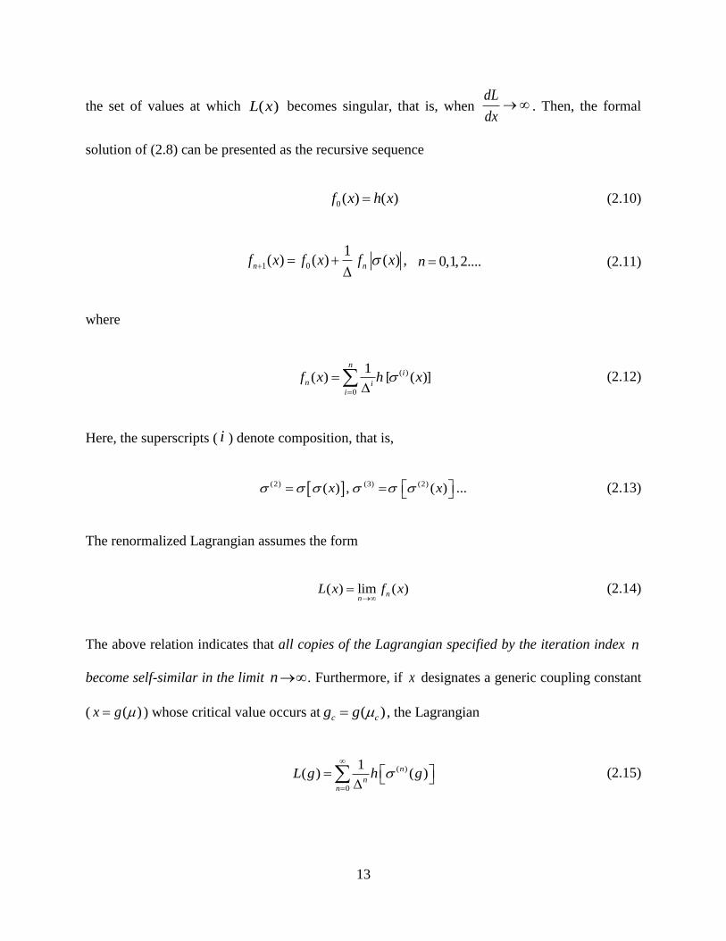
the set of values at which ( )L x becomes singular, that is, when dL

dx . Then, the formal

solution of (2.8) can be presented as the recursive sequence

0( ) ( )f x h x (2.10)

1 0

1( ) ( ) ( ) ,n nf x f x f x

0,1,2....n (2.11)

where

( )

0

1( ) [ ( )]

ni

n ii

f x h x

(2.12)

Here, the superscripts ( i ) denote composition, that is,

(2) (3) (2)( ) , ( ) ...x x (2.13)

The renormalized Lagrangian assumes the form

( ) lim ( )nn

L x f x

(2.14)

The above relation indicates that all copies of the Lagrangian specified by the iteration index n

become self-similar in the limit n. Furthermore, if x designates a generic coupling constant

( ( )x g ) whose critical value occurs at ( )c cg g , the Lagrangian

( )

0

1( ) ( )n

nn

L g h g

(2.15)

14

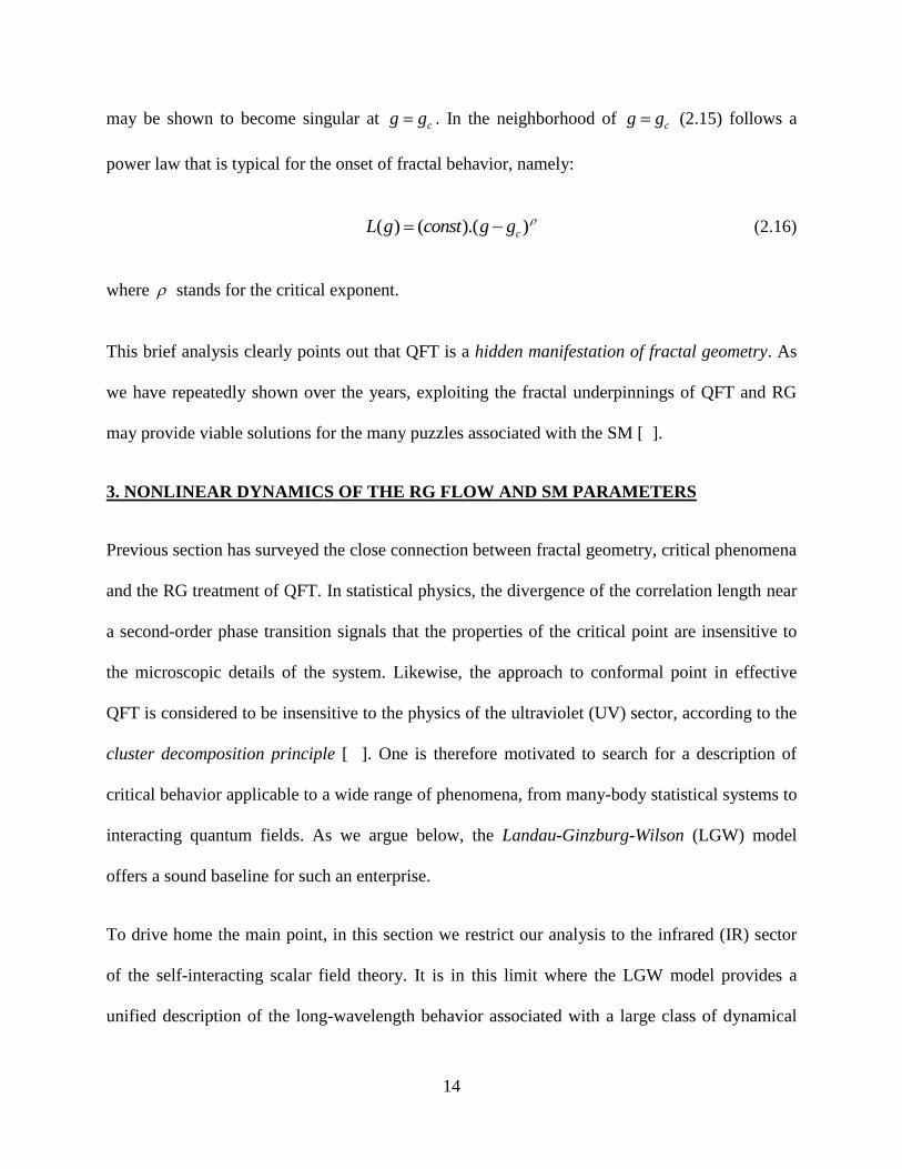
may be shown to become singular at cg g . In the neighborhood of cg g (2.15) follows a

power law that is typical for the onset of fractal behavior, namely:

( ) ( ).( )cL g const g g (2.16)

where stands for the critical exponent.

This brief analysis clearly points out that QFT is a hidden manifestation of fractal geometry. As

we have repeatedly shown over the years, exploiting the fractal underpinnings of QFT and RG

may provide viable solutions for the many puzzles associated with the SM [ ].

3. NONLINEAR DYNAMICS OF THE RG FLOW AND SM PARAMETERS

Previous section has surveyed the close connection between fractal geometry, critical phenomena

and the RG treatment of QFT. In statistical physics, the divergence of the correlation length near

a second-order phase transition signals that the properties of the critical point are insensitive to

the microscopic details of the system. Likewise, the approach to conformal point in effective

QFT is considered to be insensitive to the physics of the ultraviolet (UV) sector, according to the

cluster decomposition principle [ ]. One is therefore motivated to search for a description of

critical behavior applicable to a wide range of phenomena, from many-body statistical systems to

interacting quantum fields. As we argue below, the Landau-Ginzburg-Wilson (LGW) model

offers a sound baseline for such an enterprise.

To drive home the main point, in this section we restrict our analysis to the infrared (IR) sector

of the self-interacting scalar field theory. It is in this limit where the LGW model provides a

unified description of the long-wavelength behavior associated with a large class of dynamical

15

systems [ ]. Despite the fact the LGW model is not a realistic substitute for relativistic QFT and

the SM, it gives valuable insight into how dynamics evolves near criticality. With these

cautionary remarks in mind, the LGW model provides an effective benchmark for understanding

the primary attributes of IR quantum electrodynamics (QED) or UV quantum chromodynamics

(QCD) and asymptotically free theories.

This section is divided into two parts. In paragraph 3.1 we introduce the mapping theorem which

establishes a useful analogy between scalar field theory and the IR sector of the Yang-Mills

theory. Next paragraph develops the nonlinear dynamics of RG flow equations which are found

to provide a straightforward explanation on the hierarchical pattern of SM parameters.

3.1 THE MAPPING THEOREM

The electroweak group of the SM is represented by (2) (1)SU U and is broken at a scale

approximately given by 1

2( )EW FM O G

, in which FG is the Fermi constant [ ]. Yang-Mills

fields associated with (2)SU are vectors denoted as ( )aA x , in which 0,1,2,3 is the Lorentz

index and 1,2,3a is the group index. To manage the large number of equations derived from

the Yang-Mills theory, it is desirable to devise a method whereby ( )aA x are reduced to analog

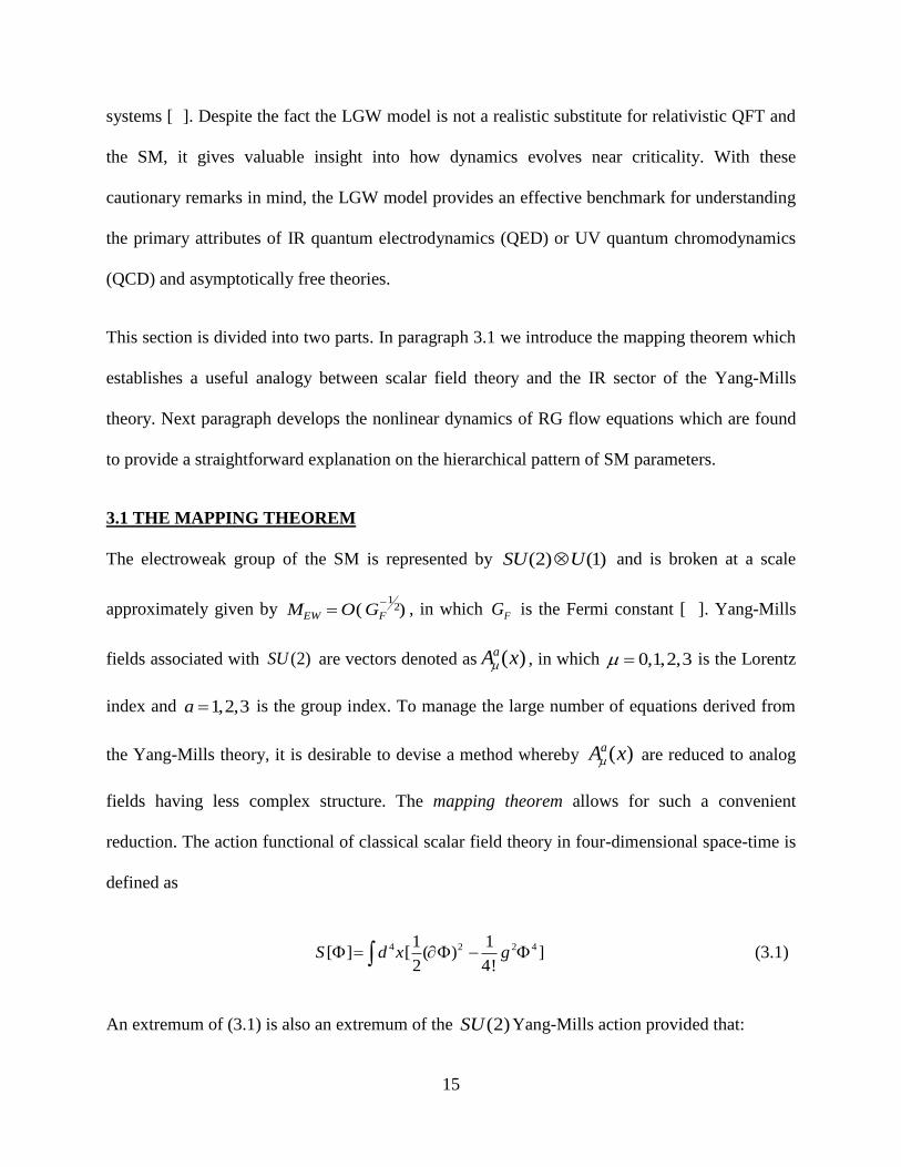
fields having less complex structure. The mapping theorem allows for such a convenient

reduction. The action functional of classical scalar field theory in four-dimensional space-time is

defined as

4 2 2 41 1[ ] [ ( ) ]

2 4!S d x g (3.1)

An extremum of (3.1) is also an extremum of the (2)SU Yang-Mills action provided that:

16

a) g represents the coupling constant of the Yang-Mills field,

b) some components of ( )aA x are chosen to vanish and others to equal each other.

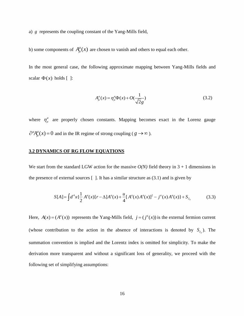
In the most general case, the following approximate mapping between Yang-Mills fields and

scalar ( )x holds [ ]:

1

( ) ( ) ( )2

a aA x x Og

(3.2)

where a

are properly chosen constants. Mapping becomes exact in the Lorenz gauge

( ) 0aA x and in the IR regime of strong coupling ( g ).

3.2 DYNAMICS OF RG FLOW EQUATIONS

We start from the standard LGW action for the massive O(N) field theory in 3 + 1 dimensions in

the presence of external sources [ ]. It has a similar structure as (3.1) and is given by

0

4 21[ ] { ( )[ ] ( ) [ ( ) ( )] ( ) ( )}

2 4

a a a a a a

J

uS A d x A x r A x A x A x j x A x S (3.3)

Here, ( ) ( ( ))aA x A x represents the Yang-Mills field, ( ( ))aj j x is the external fermion current

(whose contribution to the action in the absence of interactions is denoted by 0JS ). The

summation convention is implied and the Lorentz index is omitted for simplicity. To make the

derivation more transparent and without a significant loss of generality, we proceed with the

following set of simplifying assumptions:

17

A3.1) the LGW model is placed on a MFM characterized by a space-time dimension arbitrarily

close to four, that is, 4D , where << 1 . According to the philosophy of critical

phenomena in continuous dimension, is regarded as the sole control parameter driving the

dynamics of the model [ ]. With reference to (1.8), fine-tuning the dimensional parameter is

formally equivalent to applying continuous changes of the momentum cutoff UV . The passage

to the classical limit 0 can be approached in two separate ways:

1) UV and 0 < m << ;

2) UV < and 0m .

The latter condition matches the infrared behavior of the LGW model, i.e. its long-wavelength

properties ( ) ( )Q O m O , in which Q stands for the magnitude of momentum transfer. We

exclusively focus below on this asymptotic regime, whereby m ~ > 0.

Both limits 1) and 2) are disfavored by our current understanding of the far UV and the far IR

boundaries of field theory (see e.g. [ ]). Theory and experimental data alike tell us that the

notions of infinite or zero energy are, strictly speaking, meaningless. This is to say that either

infinite energies (point-like objects) or zero energy (infinite distance scales) are unphysical

idealizations. Indeed, there is always a finite cutoff at both ends of either energy or energy

density scale (far UV = Planck scale, far IR = finite radius of the observable Universe or the non-

vanishing energy density of the vacuum set by cosmological constant). These observations are

also consistent with the estimated infinitesimal (yet non-vanishing) photon mass, as highlighted

in [ ].

18

A3.2) In light of the mapping theorem introduced in section 4.1, the discussion is limited to the

O(1) model, i.e. the gauge field is treated as a scalar.

A3.3) the overall fermion current contains two terms,

0( ) ( ) ( )J x j x J x (3.4)

where ( )j x represents he component that couples to ( )A x and 0( )J x the free (non-interacting)

component. If ( )j x is uniform, its contribution to the action may be presented as

0( ) d

jS j A x d x jA (3.5)

Likewise, if we further assume that 0( )J x is uniform as well, its contribution to the action is well

approximated by an additive constant, that is [ ],

0JS ~ 3

0J d x ~ 3 3

0 0 ( )J J O m (3.6)

The action functional assumed the familiar form

0

4 41[ ] { ( )[ ] ( ) [ ( )] ( ) ( )}

2 4J

uS A d x A x r A x A x j x A x S (3.7)

A3.4) Section 3.1 has pointed out the close analogy between quantum field theory (QFT) and

statistical systems near criticality. On this basis, we assume that the Yang-Mills model is

reasonably well approximated by the LGW theory of critical behavior.

19

A3.5) It follows from A3.4) that the dimensional parameter of LGW theory and dimensional

regulator of Yang-Mills theory 4 D are identical entities. This identity is made explicit in

the first row of Tab. 1 below.

A3.6) As stated above, we focus on the IR regime of Yang-Mills theory in which 1

2EW FG

stands for the EW scale, FG for the Fermi constant ( )O m for the running scale and the

ultraviolet (UV) scale UV EW for the cutoff.

A3.7) The UV cutoff is not uniquely determined but smeared out by high-energy noise [ ]. The

UV cutoff spans a range of values

UV UV (3.8)

(3.8) implies that, at any given and UV , dimensional parameter falls in the range

2 UV

UV

(3.9)

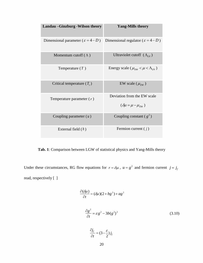
Elaborating from these premises leads to the following side-by-side comparison between the

parameters of LGW of statistical physics and Yang-Mills theory:

20

Landau –Ginzburg -Wilson theory Yang-Mills theory

Dimensional parameter ( 4 D ) Dimensional regulator ( 4 D )

Momentum cutoff ( ) Ultraviolet cutoff ( UV )

Temperature (T ) Energy scale ( EW UV )

Critical temperature ( cT ) EW scale ( EW )

Temperature parameter ( r ) Deviation from the EW scale

( EW )

Coupling parameter (u ) Coupling constant (2g )

External field ( h ) Fermion current ( j )

Tab. 1: Comparison between LGW of statistical physics and Yang-Mills theory

Under these circumstances, RG flow equations for r , 2u g and fermion current fj j

read, respectively [ ]

2 2( )( )(2 )bg ag

t

2

2 2 23 ( )g

g b gt

(3.10)

(3 )2

f

f

jj

t

21

Here,

2

43 UVa K , 43b K , 2 1

4 (8 )K (3.11)

On account of ( ), the Wilson-Fisher (WF) fixed point of (3.10) is defined by the pair

( )*6

a

b (3.12a)

2( )*

3g

b

(3.12b)

(3.12) acts as a non-trivial attractor of the RG flow. Because it resides on the critical line

EW , it describes by definition a massless field theory ( 0r ) [ ]. The non-vanishing

vacuum of at the WF point results from minimization of (3.7), that is,

1

242

6(- )v = 3( )

( )UVK

g

(3.13)

( ) and ( ) show how massive gauge bosons develop at the WF point from critical behavior near

4D . Let v =M denote the mass acquired by the gauge boson. Combining ( ), ( ), ( ) and ( )

yields

2 * 2 2( ) .EWg M const

(3.14)

* 2( )g ~ fm~

22

in which * ( )f fm O j stands for the normalized fermion mass [ ]. On account of the above

assumptions, the WF attractor ( ) changes from a single isolated point to a distribution of points.

Our next step is to explore the link between the structure of the WF attractor and the parameters

of SM.

3.3 WILSON-FISHER ATTRACTOR AS SOURCE OF PARTICLE MASSES AND

GAUGE CHARGES

We are now ready to analyze the dynamics of ( ) using the standard methods employed in the

study of nonlinear systems [ ]. To this end, we first note that the last equation in ( ) is uncoupled

to the first two. This enables us to reduce ( ) to a planar system of differential equations. We

next cast ( ) in the form of a two-dimensional map, namely

2 2 2

1( ) (1 )( ) 3 ( )n n ng t g b t g (3.15)

2 2

1( ) ( ) [1 2 ( ) ] ( )n n n nt b t g a t g (3.16)

where t represents the increment of the sliding scale. Linearizing (22) and computing its

Jacobian J gives

1 (2 ) 1J t (3.17)

It follows that the map (3.15, 3.16) is dissipative for 0 and asymptotically conservative in

the limit 0t . Invoking universality arguments [ ] we conclude that, near criticality, (3.15,

3.16) shares the same universality class with the quadratic map. Furthermore, in the

neighborhood of the Feigenbaum attractor, approaches 0 according to:

23

n

n na

(3.18)

Here, 1n is the index counting the number of cycles generated through the period doubling

cascade, is the rate of convergence (in general, different from Feigenbaum’s constant for the

quadratic map) and na is a coefficient which becomes asymptotically independent of n , that is,

a a [ ]. Substituting ( ) in ( ) yields

2 2( ) ( ) ( )n

j n n f nP n M g m

if 1n (3.19)

in which 1,2,3j indexes the three entries of (3.19). Period-doubling cycles are characterized

by 2pn , with 1p . The ratio of two consecutive terms in (3.19) is then given by

( 2 )( 1)

[ ]( )

pj

j

P pO

P p

(3.20)

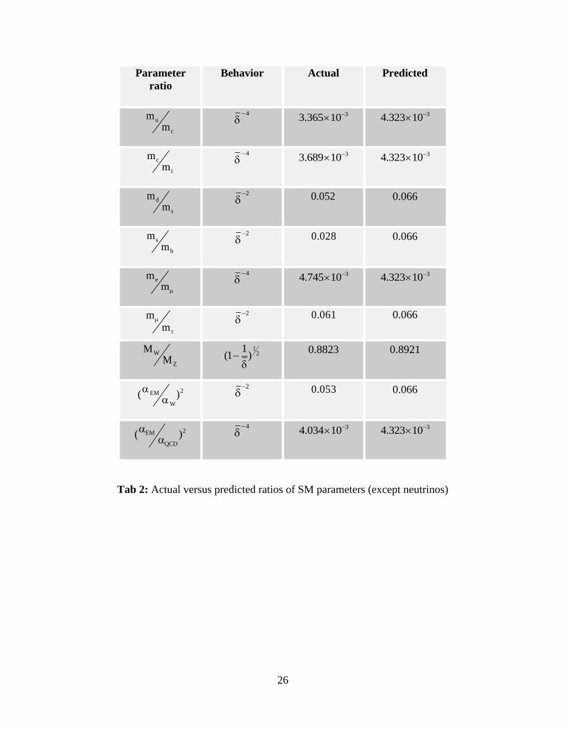
Numerical results derived from (3.20) are displayed in Tab. 3. This table contains a side-by-side

comparison of estimated versus actual mass ratios for charged leptons and quarks and a similar

comparison of coupling strength ratios. Tab. 2 contains the set of known quark and gauge boson

masses as well as the SM coupling strengths. All quark masses are reported at the energy scale

given by the top quark mass and are averaged using reports issued by the Particle Data Group [

]. Gauge boson masses are evaluated at the EW scale and the coupling strengths at the scale set

by the mass of the Z boson. The best-fit rate of convergence is 3.9 which falls close to the

numerical value of the Feigenbaum constant corresponding to hydrodynamic flows [ ]. ( ) and (

) imply that there is a series of terms containing massive electroweak bosons, namely

24

2 2 2

1 1( ) ( ) .... ( ) ... .n n n n n q n qM g M g M g const

(3.21)

For the first two terms of this series we obtain

2 2 2

2

2 2

2 2

1Z EM

W

M g e

M g

(3.22)

in which 2

4EMe

is the electromagnetic coupling strength and

2

22 4

g

the strength of

the weak interaction. The rationale for (3.22) lies in the fact that the charged gauge boson W

carries a superposition of weak and electromagnetic charges, whereas the neutral gauge boson

0Z carries only the weak isospin charge. Inverting (3.22) and taking into account the last rows of

Table 3, leads to

2

2

2

2

1 1 11 cos

111

WW

EMZ

M

M

(3.23)

(3.23) suggests a natural explanation for the Weinberg angle W . Likewise, we may write (3.22)

as

2 2 2

2 2

2 2

W Z

g g econst

M M

(3.24)

This relation offers a straightforward interpretation for both Fermi constant and the mass of the

hypothetical Higgs boson. Indeed, in SM we have [ ]

2

2

24 2 F

W

gG

M (3.25)

25

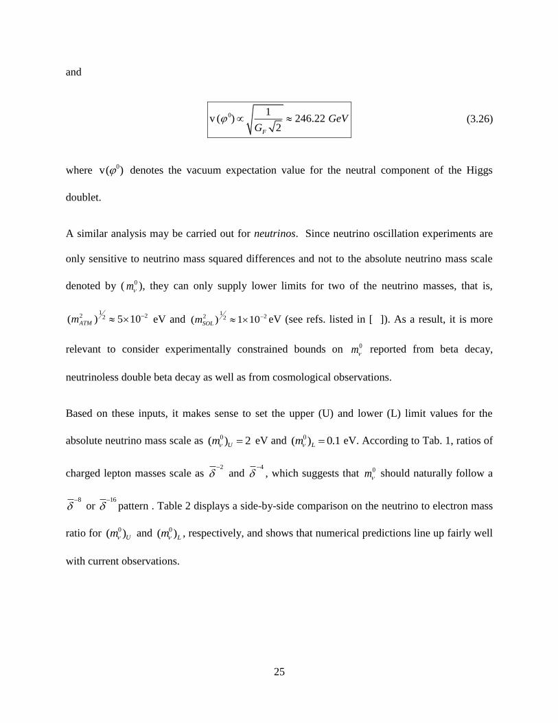
and

0 1

v ( ) 246.222F

GeVG

(3.26)

where 0v( ) denotes the vacuum expectation value for the neutral component of the Higgs

doublet.

A similar analysis may be carried out for neutrinos. Since neutrino oscillation experiments are

only sensitive to neutrino mass squared differences and not to the absolute neutrino mass scale

denoted by ( 0m), they can only supply lower limits for two of the neutrino masses, that is,

12 22( ) 5 10ATMm eV and

12 22( ) 1 10SOLm eV (see refs. listed in [ ]). As a result, it is more

relevant to consider experimentally constrained bounds on 0m reported from beta decay,

neutrinoless double beta decay as well as from cosmological observations.

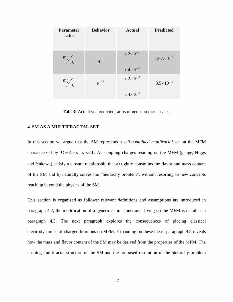
Based on these inputs, it makes sense to set the upper (U) and lower (L) limit values for the

absolute neutrino mass scale as 0( ) 2Um eV and 0( ) 0.1Lm eV. According to Tab. 1, ratios of

charged lepton masses scale as 2

and 4

, which suggests that 0m should naturally follow a

8

or 16

pattern . Table 2 displays a side-by-side comparison on the neutrino to electron mass

ratio for 0( )Um and 0( )Lm , respectively, and shows that numerical predictions line up fairly well

with current observations.

26

Tab 2: Actual versus predicted ratios of SM parameters (except neutrinos)

Parameter

ratio

Parameter

ratio

Behavior

Behavior

Actual

Actual

Predicted

Predicted

u

c

mm

4

33.365 10 34.323 10

c

t

mm

4

33.689 10 34.323 10

d

s

mm

2

0.052 0.066

s

b

mm

2

0.028 0.066

emm

4

34.745 10 34.323 10

mm

2

0.061 0.066

W

Z

MM

12

1(1 )

0.8823 0.8921

2EM

W

( )

2

0.053 0.066

2EM

QCD

( )

4

34.034 10 34.323 10

27

Parameter

ratio

Parameter

ratio

Behavior

Behavior

Actual

Actual

Predicted

Predicted

0

e

mm

8

72 10

64 10

51.87 10

0

e

mm

16

72 10

64 10

103.5 10

Tab. 3: Actual vs. predicted ratios of neutrino mass scales.

4. SM AS A MULTIFRACTAL SET

In this section we argue that the SM represents a self-contained multifractal set on the MFM

characterized by 4 , 1D . All coupling charges residing on the MFM (gauge, Higgs

and Yukawa) satisfy a closure relationship that a) tightly constrains the flavor and mass content

of the SM and b) naturally solves the “hierarchy problem”, without resorting to new concepts

reaching beyond the physics of the SM.

This section is organized as follows: relevant definitions and assumptions are introduced in

paragraph 4.2; the modification of a generic action functional living on the MFM is detailed in

paragraph 4.3. The next paragraph explores the consequences of placing classical

electrodynamics of charged fermions on MFM. Expanding on these ideas, paragraph 4.5 reveals

how the mass and flavor content of the SM may be derived from the properties of the MFM. The

ensuing multifractal structure of the SM and the proposed resolution of the hierarchy problem

28

form the topic of paragraphs 4.6 and 4.7. Two Appendix sections are included to make the paper

self-contained.

4.1 DEFINITIONS AND ASSUMPTIONS

A4.1) The cross-over regime between 0 and 0 is the only sensible setting where the

dynamics of interacting fields is likely to asymptotically approach all consistency requirements

imposed by QFT and the SM [ ]. Large deviations from four dimensions ( ~ (1)O ) may signal

the breakdown of these requirements. Particular attention needs to be paid, for example, to the

potential violation of Lorentz invariance in Quantum Gravity theories advocating the emergence

of space-time of lower dimensionality at high energy scales [ ].

From the standpoint of interacting field theory, a non-vanishing and arbitrarily small deviation

from four dimensions is equivalent to allowing the Renormalization Group (RG) equations to

slide outside the isolated fixed points solutions (FP) [ ]. Recalling that FP are synonymous with

equilibria in the dynamical systems theory, it follows that, in general, the evolution of quantum

fields is no longer required to settle down to equilibrium states. The end result is that the

condition 1 enables the isolated FP of the RG equations to morph into attractors with a

more complex structure [ ].

A4.2) 0u is the reference charge distribution on MFM for a fixed 1 (fixed number of

dimensions),

A4.3) u is the effective charge distribution on MFM when 1 is allowed to vary (i.e., the

number of dimensions is allowed to evolve with the energy scale),

29

A4.4) 0 0 0,, , fg y are the coupling charges for the scalar, gauge and Yukawa sectors of the

Standard Model, measured at the energy of the electroweak scale defined by EWM in ordinary

four dimensional space-time ( 0 ).

A4.5) Any theory exploring physics beyond the Standard Model (BSM) must fully recover the

principles and the framework of perturbative QFT at energy scales approaching EWM . In

particular, it needs to preserve unitarity, renormalizability and local gauge invariance and be

compatible with precision electroweak data [ ].

4.3 THE MINIMAL FRACTAL MANIFOLD (MFM)

Field theory on fractional four-dimensional space-time is described by the action

4( ) (v( ) )S d x L x d x L

(4.1)

where the measure ( )d x denotes the ordinary four-dimensional volume element multiplied by a

weight function v( )x [ ]. If the weight function is factorizable in coordinates and positive

semidefinite, v( )x assumes the form

13

0

v( )( )

xx

(4.2)

in which

0 1 (4.3)

30

are four independent parameters. An isotropic space-time of dimension 4D is

characterized by

14

(4.4)

which turns (4.2) into

v( )x ≈ 4

( )x (4.5)

Dimensional analysis requires all coordinates entering (4.2) and (4.5) to be scalar quantities.

They can be generically specified relative to a characteristic length and time scale, as in

0

0

xx

L

(4.6)

in which 0, are positive-definite energy scales. Relation (4.5) becomes

4

0

v( ) ( )x

(4.7)

such that

0

0, 0lim v( )

, 0x

ifx

if

(4.8)

Choosing 0 we can expand (4.7) as:

lnaa e ≈ 1 ln a (4.9)

31

which yields

0

v( ) 1 4 ln( ) 1 4 ln( )x x

(4.10)

4.4 EMERGENCE OF EFFECTIVE FIELD CHARGES ON THE MFM

A remarkable property of fractal space-time is the emergence of “effective” coupling charges

induced by polarization in non-integer dimensions [ ]. To fix ideas, consider the case of classical

electrodynamics coupled to spinor fields in a MFM with evolving dimensionality [ ]. From

(4.10) we obtain

2

2

0v( )e x e ≈ 2

0

0

1 4 ln( )

e

(4.11)

where, following definitions A4.2) and A4.3),

0 0,e u e u

In light of assumption A4.5), (4.11) has to match the expression of the running charge in

perturbative Quantum Electrodynamics (QED). At one loop, this expression reads [ ]

2

2 0

2

0

2

0

1 ln( )6

ee

e

(4.12)

Comparing (4.11) with (4.12) leads to:

2

0 ( )e O (4.13)

32

This finding reveals that the dimensional parameter represents the physical source of the field

charge in ordinary four-dimensional space-time. As previously alluded to, this “dynamic

generation” of effective field charges can be traced back to the intrinsic polarization induced by

fractal space-time. The process is strikingly similar to the emergence of non-trivial FP’s in the

LGW model of critical behavior in 4D dimensions [ ]. The discussion may be

extrapolated from electrodynamics to classical gauge theory and, as we show next, it sets the

stage for a novel interpretation of mass and flavor hierarchies present in the SM.

4.5 THE MASS AND FLAVOR HIERARCHIES OF THE SM

Re-iterating results obtained in section 3.3, the analysis of the RG equations on the MFM reveals

that, near the electroweak scale, the normalized masses of fermions ( fm ), weak bosons ( M ) and

electroweak gauge charges ( 0g ) scale as

fm ~ (4.14)

2

0g ~ (4.15)

2 2 2

0g M const M ~ 1 (4.16)

It can be also shown that, under some generic assumptions regarding the RG flow and its

boundary conditions, the system of RG equations lead in general to a transition to chaos via

period-doubling bifurcations as 0 [ ]. According to ideas outlined in section 3, the

sequence of critical values , 1,2,...n n driving this transition to chaos satisfies the geometric

progression

33

0n n ~ n

nk

(4.17)

Here, 1n is the index counting the number of cycles created through the period-doubling

cascade, is the rate of convergence and nk is a coefficient that becomes asymptotically

independent of n as n . Period-doubling cycles are characterized by 2in , for i >> 1.

Substituting (4.17) in (4.14) and (4.15) yields the following ladder-like progression of critical

couplings

,f im ~ 2

0,ig ~ 2 i

(4.18a)

In section 3.3 we found that scaling (4.18a) recovers the full mass and flavor content of the SM,

including neutrinos, together with the coupling strengths of gauge interactions. Specifically,

The trivial FP of the RG equations consists of the massless photon ( ) and the massless

UV gluon ( g ).

The non-trivial FP of the RG equations is degenerate and consists of massive quarks ( q ),

massive charged leptons and their neutrinos ( ,l ) and massive weak bosons ( ,W Z ).

Gauge interactions develop near the non-trivial FP and include electrodynamics, the weak

interaction and the strong interaction.

It was suggested in [ ] that a space-time background with low-level fractality ( <<1) favors the

formation of a Higgs-like condensate of gauge bosons, as in

0 01 [( ) ( )]4C W W Z g W W Z g (4.18b)

34

Here, 0,W Z denote the triplet of massive (2)SU bosons and ,g stand for gluon and photon,

respectively. Relation (4.18b) implies that the scalar condensate C acquires a mass in close

agreement with the mass of the SM Higgs boson ( Hm = 125.6GeV ).

4.6 MULTIFRACTAL STRUCTURE OF THE SM

A key parameter of the RG analysis is the dimensionless ratio ( )UV

, in which is the sliding

scale and UV >> the high-energy cutoff of the underlying theory. As discussed in the first

section, the connection between the parameter 4 D and UV is given by

~ 2

2

1

log ( )UV

(4.19)

The large numerical disparity between and UV enables one to approximate as in

~ 2( )UV

(4.20)

Let im denote the full spectrum of particle masses present in the SM. Relation (4.20) can be

written as

2 22 2

02 2( )i i EW

i i

UV EW UV

m m Mr

M

(4.21)

in which

2

0 2,i EW

i

EW UV

m Mr

M

(4.22)

35

and

2

0

iir

(4.23)

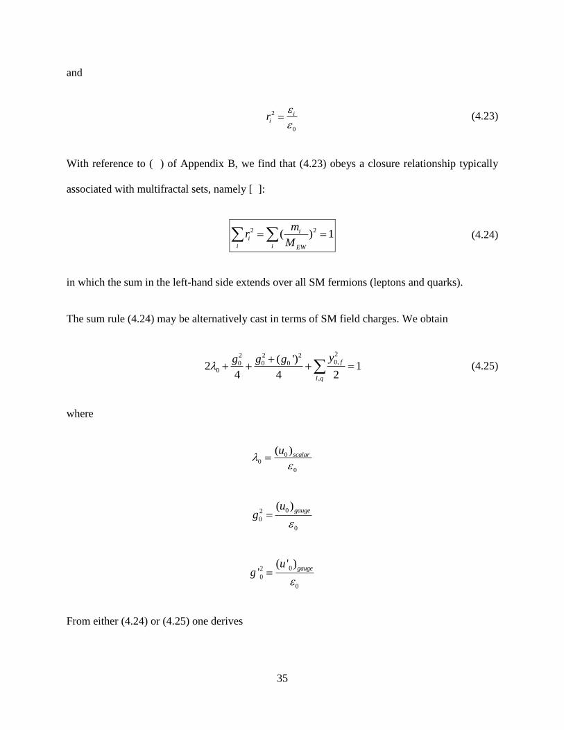
With reference to ( ) of Appendix B, we find that (4.23) obeys a closure relationship typically

associated with multifractal sets, namely [ ]:

2 2( ) 1i

i

i i EW

mr

M (4.24)

in which the sum in the left-hand side extends over all SM fermions (leptons and quarks).

The sum rule (4.24) may be alternatively cast in terms of SM field charges. We obtain

22 2 20,0 0 0

0

,

( ')2 1

4 4 2

f

l q

yg g g

(4.25)

where

00

0

( )scalaru

02

0

0

( )gaugeug

02

0

0

( ' )'

gaugeug

From either (4.24) or (4.25) one derives

36

EWM ~ V = 246.2 GeV (4.26)

in close agreement with the vacuum expectation value of the SM Higgs boson (V ). In closing,

we mention that the existence of (4.25) was first brought up in [ ], with no attempt of

formulating a theoretical interpretation.

4.7 SOLVING THE FLAVOR AND HIERARCHY PROBLEMS ON THE MFM

Relations (4.18), (4.24) and (4.25) tightly constrain the particle content of the SM. They

naturally fix its number of independent field flavors near the electroweak scale. Also, since all

scaling ratios in (4.24) must have a magnitude of less than one unit, (4.24) and (4.25) necessarily

imply that the mass of the Higgs boson cannot grow beyond EWM , at least near the electroweak

scale. This conclusion brings closure to the hierarchy problem, whose formulation is briefly

outlined in Appendix B.

5. MFM AND THE DYNAMIC GENERATION OF MASS SCALES IN FIELD THEORY

The consensus among high-energy theorists is that, as of today, the mechanism underlying the

generation of mass scales in field theory remains elusive. Our intent here is to point out that the

MFM can naturally account for the onset of these scales. A counterintuitive outcome of this

analysis is the deep link between the minimal fractal manifold and the holographic principle.

5.1 MOTIVATION

One of the many unsettled questions raised by field theory revolves around the vast hierarchy of

scales in Nature [ ]. A large numerical disparity exists between the Planck scale ( PlM ), the

37

electroweak scale ( EWM ), the hadronization scale of Quantum Chromodynamics (QCD ) and the

cosmological constant scale (1

4cc , with cc expressed as energy density in 3+1 dimensions).

It has been long known that perturbative QFT cannot provide a complete description of Nature

since its formalism entails divergences at both ends of the energy spectrum [ ]. For instance,

many textbooks emphasize that the singular behavior of momentum integrals in the ultraviolet

(UV) sector arises from the poorly understood space-time structure at short distances [ ]. Lattice

field models handle infinities through discretization of the space-time continuum on a grid of

spacing " " . This procedure naturally bounds the maximal momentum allowed to propagate

through the lattice, namely,

p ≤ maxp ~ 1(2 ) (5.1)

The downside of lattice models is that they generally fail to be either gauge or Poincaré invariant

[ ]. Restoring formal consistency is further enabled via the RG program [ ]. RG regulates the n-

th order momentum integrals of the generic form

2( ) ( )n

nI p dp f p (5.2)

by either inserting an arbitrary momentum cutoff 0 < ~1 < or by continuously

“deforming” the four-dimensional space-time via the dimensional parameter . The resulting

theory is free from divergences and operates with a finite number of redefined physical

parameters. Restoring the continuum space-time limit is done at the end by taking the limit

or 0 . Both limits are disfavored by experimental data, as discussed in section…

38

Reinforcing this viewpoint, some authors argue that the idea of smooth space-time stands in

manifest conflict with the basic premises of quantum theory [ ]. To confine an event within a

region of extension requires a momentum transfer on the order of 1 which, in turn,

generates a local gravitational field. If the density of momentum transfer is comparable in

magnitude with the right hand side of Einstein’s equation, the local curvature of space-time (~

2

0R ) induced by this transfer is given by (in natural units, 1c )

2

0R ~

4

NG (5.3)

However, collapse of the event within a short region of extent 0( )O R amounts to trapping

outgoing light signals and preventing direct observation.

All these considerations invariably point to the following challenge: on the one hand, a

continuum model of space-time near or below EWM serves as an effective paradigm that is likely

to fail at large probing energies. Yet on the other, any discrete model of space-time typically

violates Poincaré or gauge symmetries. It seems only natural, in this context, to take a fresh look

at ( ) and ( ) and appreciate the message it conveys: if either UV stays finite or << 1 is

arbitrarily small but non-vanishing, space-time dimensionality becomes a non-integer arbitrarily

close to four. Stated differently, in the neighborhood of EWM , conventional space-time

necessarily turns into a MFM [ ].

On closer examination, this finding is hinted by a number of alternative theoretical arguments:

a) It is well known that the principle of general covariance lies at the core of classical relativistic

field theory. An implicit assumption of general covariance is that any coordinate transformation

39

and its inverse are smooth functions that can be differentiated arbitrarily many times. However,

as it is also known, there is a plethora of non-differentiable curves and surfaces in Nature, as

repeatedly discovered since the introduction of fractal geometry in 1983 [ ]. The unavoidable

conclusion is that relativistic field theory assigns a preferential status to differentiable

transformations and the smooth geometry of space-time, which is at odds with the very spirit of

general covariance.

b) On the mathematical front, significant effort was recently invested in the development of q-

deformed Lie algebras, non-commutative field theory, quantum groups, fractional field theory

and its relationship to the MFM [ ]. It is instructive to note that all these contributions appear to

be directly or indirectly related to fractal geometry [ ]. Moreover, the condition << 1, defined

within the framework of MFM, is the sole sensible setting where fractal geometry asymptotically

approaches all consistency requirements mandated by QFT and the Standard Model [ ].

c) Demanding that phenomena associated with gravitational collapse follow the postulates of

quantum theory implies that the world is no longer four-dimensional near PlM . This statement

has lately received considerable attention and forms the basis for dimensional reduction and for

the holographic principle of Quantum Gravity theories [ ]. If we accept that the four-

dimensional continuum is an emergent property of the electroweak scale and below ( < EWM ),

the holographic principle implies that space-time dimensionality evolves with the energy scale

between EWM , where << 1, and PlM , where space is expected to become two-dimensional

viz. (1)O [ ].

Our paper is organized as follows: next section introduces the concept of holographic bound and

derives the relationship involving the IR and UV cutoffs of field theory. Building on these

40

premises, section 5.3 presents a comparison between mass scales estimated using our approach

and their currently known values.

5.2 THE HOLOGRAPHIC BOUND

Consider an effective QFT confined to a space-time region with characteristic length scale L and

assume that the theory makes valid predictions up to an UV cutoff scale UV >> 1L . It can be

shown that the entropy associated with this effective QFT takes the form [ ]

S ~ 3 3

UV L (5.4)

To understand the significance of (5.4), consider an ensemble of fermions living on a periodic

space lattice with characteristic size L and period 1

UV

. One finds that (5.4) simply follows from

counting the number of occupied states for this system, which turns out to be 3( )

2 UVLN

[ ]. The

holographic principle stipulates that (5.4) must not exceed the corresponding black hole entropy

BHS , that is,

3 3

UVL ≤ 2 2

24

BHBH Pl

Pl

AS R M

l (5.5)

in which BHA is the area of the spherical event horizon of radius R . Introducing a new reference

length scale defined as

3

2

L

R (5.6)

leads to the condition

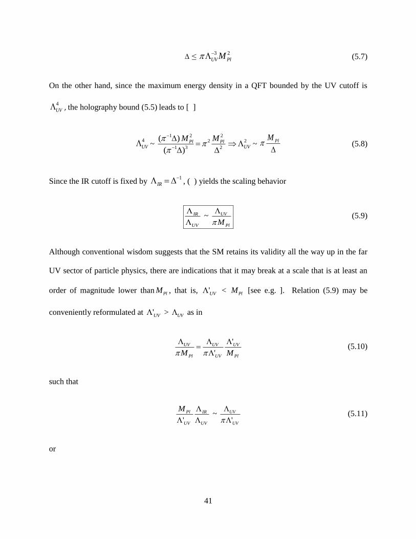
41

≤ 3 2

UV PlM (5.7)

On the other hand, since the maximum energy density in a QFT bounded by the UV cutoff is

4

UV , the holography bound (5.5) leads to [ ]

4

UV ~ 1 2 2

2 2

1 3 2

( )

( )

Pl PlUV

M M

~

PlM

(5.8)

Since the IR cutoff is fixed by 1

IR

, ( ) yields the scaling behavior

IR

UV

~ UV

PlM

(5.9)

Although conventional wisdom suggests that the SM retains its validity all the way up in the far

UV sector of particle physics, there are indications that it may break at a scale that is at least an

order of magnitude lower than PlM , that is, 'UV < PlM [see e.g. ]. Relation (5.9) may be

conveniently reformulated at 'UV > UV as in

'

'

UV UV UV

Pl UV PlM M

(5.10)

such that

'

Pl IR

UV UV

M

~

'

UV

UV

(5.11)

or

42

'IR

UV

~

'

UV

UV

(5.12)

in which 'IR > IR is a new IR scale given by

''

Pl IRIR

UV

M

(5.13)

A glance at ( ), ( ) and ( ) reveals deep similarities between the holographic principle and the

MFM. They all represent scaling relations that mix and constrain largely separated mass scales.

We next use ( ) and ( ) to derive numerical estimates and compare them with experimental data.

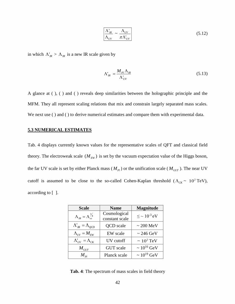
5.3 NUMERICAL ESTIMATES

Tab. 4 displays currently known values for the representative scales of QFT and classical field

theory. The electroweak scale ( )EWM is set by the vacuum expectation value of the Higgs boson,

the far UV scale is set by either Planck mass ( PlM ) or the unification scale ( GUTM ). The near UV

cutoff is assumed to be close to the so-called Cohen-Kaplan threshold ( CK ~ 210 TeV),

according to [ ].

Scale Name Magnitude

14

IR cc Cosmological

constant scale ≤ ~ 10-3 eV

'IR QCD QCD scale ~ 200 MeV

UV EWM EW scale ~ 246 GeV

'UV CK UV cutoff ~ 210 TeV

GUTM GUT scale ~ 1016 GeV

PlM Planck scale ~ 1019 GeV

Tab. 4: The spectrum of mass scales in field theory

43

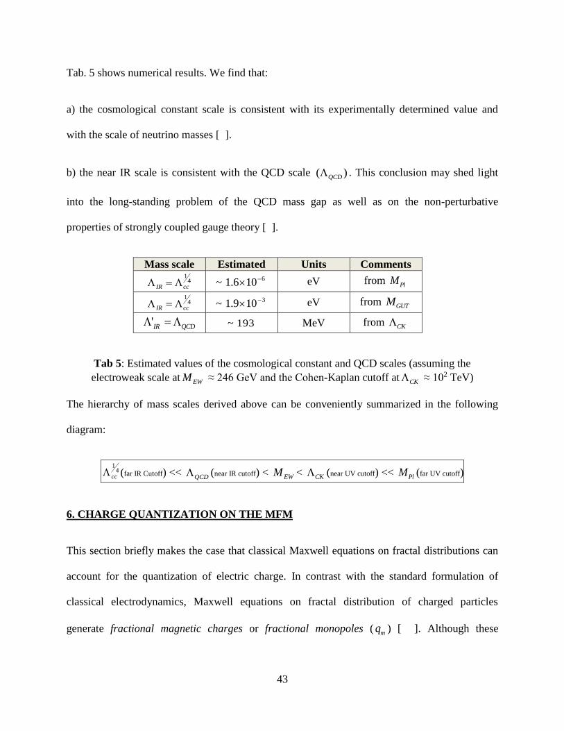
Tab. 5 shows numerical results. We find that:

a) the cosmological constant scale is consistent with its experimentally determined value and

with the scale of neutrino masses [ ].

b) the near IR scale is consistent with the QCD scale ( )QCD . This conclusion may shed light

into the long-standing problem of the QCD mass gap as well as on the non-perturbative

properties of strongly coupled gauge theory [ ].

Mass scale Estimated Units Comments 1

4IR cc ~

61.6 10 eV from PlM

14

IR cc ~ 31.9 10 eV from GUTM

'IR QCD ~ 193 MeV from CK

Tab 5: Estimated values of the cosmological constant and QCD scales (assuming the

electroweak scale at EWM ≈ 246 GeV and the Cohen-Kaplan cutoff at CK ≈ 102 TeV)

The hierarchy of mass scales derived above can be conveniently summarized in the following

diagram:

14

cc (far IR Cutoff) << QCD (near IR cutoff) < EWM < CK (near UV cutoff) << PlM (far UV cutoff)

6. CHARGE QUANTIZATION ON THE MFM

This section briefly makes the case that classical Maxwell equations on fractal distributions can

account for the quantization of electric charge. In contrast with the standard formulation of

classical electrodynamics, Maxwell equations on fractal distribution of charged particles

generate fractional magnetic charges or fractional monopoles ( mq ) [ ]. Although these

44

fractional objects are un-observable at energy scales significantly lower than EWM , their

cumulative contribution may become relevant for charge quantization following Dirac’s theory

of magnetic monopoles. Needless to say, this short analysis is far from being either rigorous or

complete. Our sole intent is opening an unexplored research avenue which, to the best of our

knowledge, has not received any prior consideration.

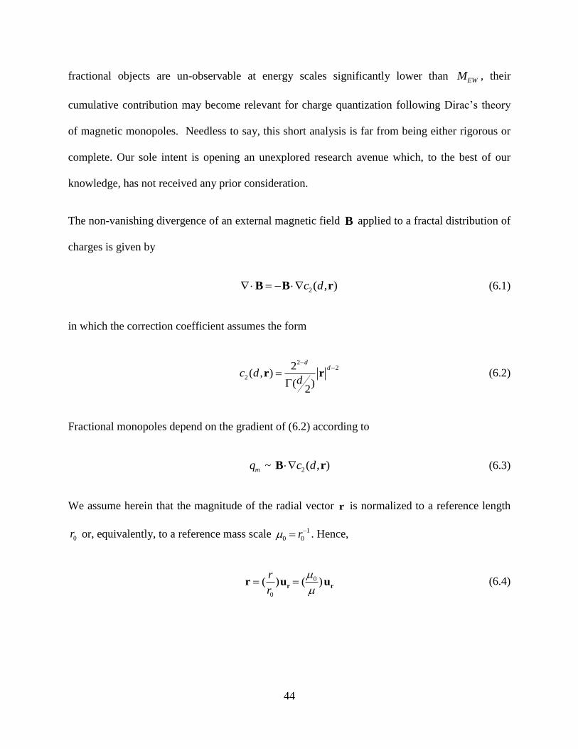
The non-vanishing divergence of an external magnetic field B applied to a fractal distribution of

charges is given by

2( , )B B rc d (6.1)

in which the correction coefficient assumes the form

2

2

2

2( , )

( )2

dd

c dd

r r (6.2)

Fractional monopoles depend on the gradient of (6.2) according to

mq ~ 2( , )c dB r (6.3)

We assume herein that the magnitude of the radial vector r is normalized to a reference length

0r or, equivalently, to a reference mass scale 1

0 0r . Hence,

0

0

( ) ( )r

r

r rr u u (6.4)

45

in which r

u stands for the unit vector in the radial direction. Since the deviation from two

dimensionality on a minimal fractal manifold is quantified as 2d , with << 1, (6.2) is

well approximated by

2( , )c d r ~ 0( )

ru (6.5)

Combined use of (6.2) and (6.5) yields

2( , )rc ~ 10

0

( ) ( )

r ru u (6.6)

Because our analysis is carried out in a classical framework, we choose 0 EWM and the

regime of mesoscopic scales << EWM , with ( )EW

OM

. Relation (6.6) turns into

2( , )rc ~ 2 ru (6.7)

The quadratic dependence on suggests that fractional magnetic charges are likely to be

unobservable on mesoscopic scales. Substituting (6.7) into the Dirac charge quantization

condition [ ] gives

meq ~ 2

n 2( )e rB u ~

2

n (6.8)

where natural units are assumed and 1, 2,...n . It is readily seen that, in contrast with

fractional magnetic charges, the quantization of free electric charges scales as 2 and is likely

to be observable at mesoscopic distances on the order of 1( )O

.

46

7. ON THE CONNECTION BETWEEN MFM AND QUANTUM SPIN

The aim of this section is to point out that the inner connection between MFM and local

conformal field theory (CFT) makes quantum spin a topological property of the MFM.

7.1 INTRODUCTORY REMARKS

In his seminal paper of 1939, Wigner has shown that the concept of quantum spin follows

naturally from the unitary representation of the Poincaré group [ ]. The two invariant Casimir

operators of the Poincaré group, 2P P m

and ( 1)W W ms s

supply the rest mass m and

the spin s of the particle, respectively. Here P is the generator of translations and W the

Pauli-Lubanski operator defined as

W P J

(7.1)

in which stands for the four-dimensional Levi-Civita index and J are the generators of

the Lorentz group. The second Casimir invariant implies that the square of the spin three-vector

of a massive particle ( S ) relates to the Pauli-Lubanski operator via

2

1S S W W

m

(7.2)

Our brief analysis reveals that quantum spin may be understood outside the traditional

framework of representation theory, specifically as emerging attribute of the MFM. Expanding

on these ideas, we next suggest that the inner connection between MFM and local conformal

field theory (CFT) makes quantum spin a topological property of the MFM. It is instructive to

47

note that this interpretation of quantum spin resonates well with the framework of ideas

presented in [S. Forte].

7.2 QUANTUM SPIN AS MANIFESTATION OF THE MFM

Consider a flat four-dimensional space-time with constant metric having the standard signature

( 1,..., 1)diag . A differentiable map ' ( )x x is called a conformal transformation if the

metric tensor changes as [ ]

2' '( )

x xx

x x

(7.3)

in which 2( )x represents the scale factor and Einstein’s summation convention is implied. The

scale factor is strictly equal to unity on flat space-times (2( ) 1x ), a condition matching the

translations and rotations group of Lorentz transformations. In general, if the underlying space-

time background deviates from flatness and is characterized by a metric ( )g x ≠ , the

condition for local conformal transformation (7.3) reads

2( ) ( ) ( ) ( )g x g x x g x (7.4)

where 2( )x ≠ 1 . A nearly conformal transformation (NCT) is defined by a scale factor

departing slightly and continuously from unity, that is,

2( ) 1 ( )x x ≈ exp[ ( )]x , ( )x << 1 (7.5)

Consider next infinitesimal coordinate transformations which, up to a first order in a small

parameter ( )x << 1 , can be presented as

48

2' ( ) ( )x x x O (7.6)

Demanding that (7.6) represents a local conformal transformation amounts to [ ]

2

( )D

(7.7)

The scale factor corresponding to (7.6) is given by

2 22( )( ) 1 ( )x O

D

(7.8)

Any locally defined MFM is characterized by a space-time dimension ( ) 4 ( )D x x , where

the onset of the fractal dimension ( )x << 1 reflects a nearly-vanishing deviation from strict

conformal invariance expected at the trivial FP’s of the RG flow [ ]. Conformal behavior in flat

space-time matches the scale-invariant (constant) metric , whereby 2( ) 1x and ( ) 0x

as a result of (7.3) and (7.5). In field-theoretic language, reaching the conformal limit on the flat

four dimensional space-time means that the RG trajectories flow into stable fixed points where

they settle down to steady equilibria. One arrives at similar conclusions by following the

prescription of the dimensional regularization program [ ]. All these observations enable us to

draw a natural connection between the fractal dimension ( )x << 1 and the NCT, namely,

2( ) 4 ( ) ( ) 1 ( )D x x x x (7.9)

Replacing (7.9) into (7.8) and ignoring the contribution of quadratic terms yields

2 ( ) ( )x x << 1 (7.10)

49

Furthermore, setting the fractal dimension as divergence of a locally defined “dimensional” field

( )x

2 ( )x

(7.11)

leads to the following condition for conformal invariance on the MFM

( ) << 1 (7.12)

A typical ansatz in CFT is to assume that the infinitesimal coordinate transformations ( )x are

at most quadratic in x , that is,

( )x a b x c x x

(7.13)

where , ,a b c << 1 are constant coefficients with c c . The individual terms of

expansion (13) describe various conformal transformations and their respective generators. In

particular,

1) The constant coefficient a represents an infinitesimal translation 'x x a whose

generator is the momentum operator P i .

2) The next term can be split into a symmetric and an anti-symmetric contribution according to

b m (7.14)

where m m . The symmetric part labels infinitesimal scale transformations

(dilatations) of the generic form ' (1 )x x and corresponding generator D ix

. The

50

anti-symmetric part m describes infinitesimal rotations ' ( )x m x

whose associated

generator is the angular momentum operator ( )L i x x .

3) The last term at the quadratic order in x defines the so-called “special conformal

transformations”.

Returning to (7.9) to (7.12), a reasonable hypothesis is to assume that the dimensional field ( )x

is at most linear in x , which corresponds to a nearly-constant fractal dimension ( )x ≈ . Thus

we take

( )x d e x (7.15)

subject to the requirement of infinitesimal coefficients ,d e << 1 . Retracing previous steps, we

split e into a symmetric and anti-symmetric contribution

e f (7.16)

subject to the condition f f . The symmetric part denotes a scale transformation similar to

' (1 )x x , whereas the anti-symmetric part defines an “intrinsic” rotation of the form

' ( )x f x

(7.17)

It follows that the “rotation-like” transformation (17) stems from the fractal topology of the

MFM and may be associated with the generator of quantum spin S . A favorable consequence

of this brief analysis is that, by construction, S replicates the algebra of the angular

51

momentum operator L . In closing we mention that these findings are consistent with the body

of ideas developed in [ ].

8. FRACTAL PROPAGATORS AND THE ASYMPTOTIC SECTORS OF QFT

This section contemplates the connection between the asymptotic regions of QFT and the MFM.

The starting point of our analysis is the observation that propagators for charged fermions no

longer follow the prescription of perturbative QFT in the far IR and far UV sectors of particle

physics. The propagators acquire a fractal structure from radiative corrections contributed by

gauge bosons. We show how this structure may be analyzed using the attributes of the MFM.

An intriguing consequence of this approach is the emergence of classical gravity as long-range

and ultra-weak excitation of the Higgs condensate.

8.1 INTRODUCTORY REMARKS

The free-fermion propagator in QFT determines the probability amplitude for a fermion to travel

between different space-time locations. It is given by [ ]

4

4( ) exp[ ( )] ( )

(2 )F F

d pS x y ip x y S p

(8.1)

in which

2 2

1( )

0 0F

p mS p

p m i p m i

(8.2)

This formula successfully applies to both the IR regime of quantum electrodynamics (QED) and

the UV limit of quantum chromodynamics (QCD), where the approximation of nearly free-

52

fermions holds well. In contrast, at distance scales where the radiative contribution of soft

photons to electron self-interaction becomes relevant and is accounted for, the propagator

changes to [ ]

2 2 (1 )

( ) ( ) (1 )( 0 )

p mmS p

i p m i

(8.3)

Here, the fractional “anomalous” exponent

is related to the low-energy value of the fine

structure constant , is an arbitrary high-energy scale and (...) stands for the Gamma

function. Surveying the history of publications on this topic reveals the limitations of

conventional QFT in dealing with non-perturbative aspects of particle physics [ ].

Let

2 2 (1 )

1 ( 0 )( ) ( )

p m iS p f

p m m

≈ ( 0 ) ( )p m i fm

(8.4a)

( )fm

( )

i

m

(8.4b)

represent the inverse propagator entering (8.3). Relation (8.4) explicitly factors out the

contribution of the standard inverse propagator ( 0 )p m i

and the interpolating function

( ) ( )ifm m

expressed in terms of two widely separated mass scales m << and fractional

exponent .

53

This analysis is, however, not limited to the QED of charged fermions. Similar reasoning

indicates that both scalar and gauge bosons of the Standard Model (SM) cannot be realistically

approximated as excitations of free fields. In particular [ ],

a) Higgs and Yang-Mills theories are nonlinear dynamic models which exhibit self-interaction,

with the possible exception of the deep UV sector where they become ultra-weakly coupled or

“trivial”.

b) In general, the contribution of fermionic loops (and hypothetical new degrees of freedom

arising beyond SM) cannot be fully balanced without invoking precise cancellation of competing

diagrams (“fine tuning”).

c) Although the SM is perturbatively renormalizable and free from anomalies, anomalous

propagators and their corresponding behavior can still occur whenever conditions fall outside

perturbation theory.

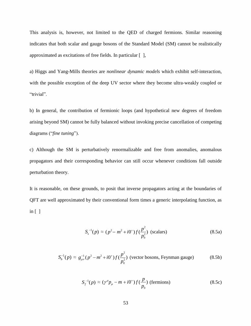
It is reasonable, on these grounds, to posit that inverse propagators acting at the boundaries of

QFT are well approximated by their conventional form times a generic interpolating function, as

in [ ]

1( )sS p

≈ 2

2 2

2

0

( 0 ) ( )p

p m i fp

(scalars) (8.5a)

1( )bS p

≈ 2

1 2 2

2

0

( 0 ) ( )p

g p m i fp

(vector bosons, Feynman gauge) (8.5b)

1( )fS p ≈ 0

( 0 ) ( )p

p m i fp

(fermions) (8.5c)

54

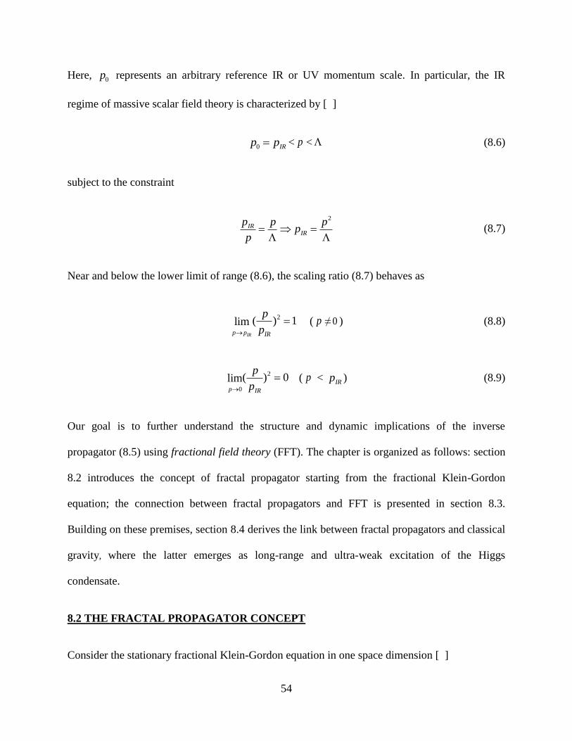
Here, 0p represents an arbitrary reference IR or UV momentum scale. In particular, the IR

regime of massive scalar field theory is characterized by [ ]

0 IRp p < p < (8.6)

subject to the constraint

2

IRIR

p p pp

p

(8.7)

Near and below the lower limit of range (8.6), the scaling ratio (8.7) behaves as

2( ) 1lim

IRp p IR

p

p

( p ≠ 0 ) (8.8)

2

0

( ) 0limp IR

p

p

( p < IRp ) (8.9)

Our goal is to further understand the structure and dynamic implications of the inverse

propagator (8.5) using fractional field theory (FFT). The chapter is organized as follows: section

8.2 introduces the concept of fractal propagator starting from the fractional Klein-Gordon

equation; the connection between fractal propagators and FFT is presented in section 8.3.

Building on these premises, section 8.4 derives the link between fractal propagators and classical

gravity, where the latter emerges as long-range and ultra-weak excitation of the Higgs

condensate.

8.2 THE FRACTAL PROPAGATOR CONCEPT

Consider the stationary fractional Klein-Gordon equation in one space dimension [ ]

55

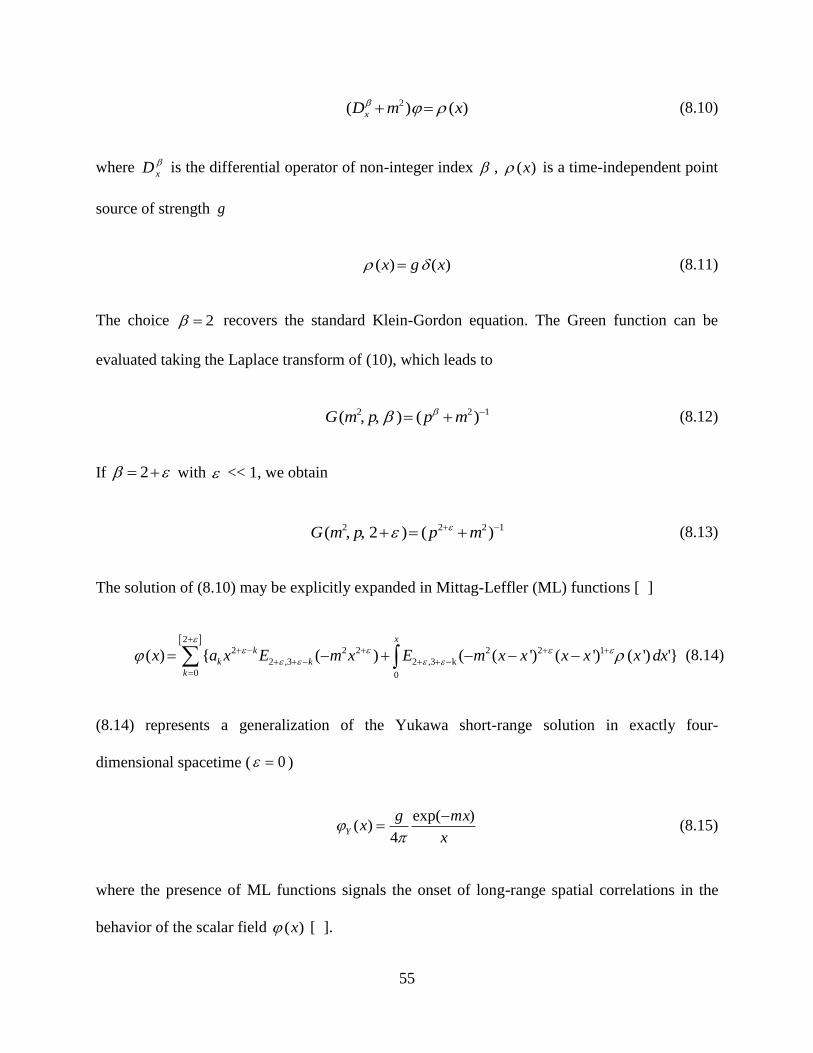
2( ) ( )xD m x (8.10)

where xD is the differential operator of non-integer index , ( )x is a time-independent point

source of strength g

( ) ( )x g x (8.11)

The choice 2 recovers the standard Klein-Gordon equation. The Green function can be

evaluated taking the Laplace transform of (10), which leads to

2 2 1( , , ) ( )G m p p m (8.12)

If 2 with << 1, we obtain

2 2 2 1( , , 2 ) ( )G m p p m (8.13)

The solution of (8.10) may be explicitly expanded in Mittag-Leffler (ML) functions [ ]

2

2 2 2 2 2 1

2 ,3 2 ,3 k

0 0

( ) { ( ) ( ( ') ( ') ( ') '}

x

k

k k

k

x a x E m x E m x x x x x dx

(8.14)

(8.14) represents a generalization of the Yukawa short-range solution in exactly four-

dimensional spacetime ( 0 )

exp( )

( )4

Y

g mxx

x

(8.15)

where the presence of ML functions signals the onset of long-range spatial correlations in the

behavior of the scalar field ( )x [ ].

56

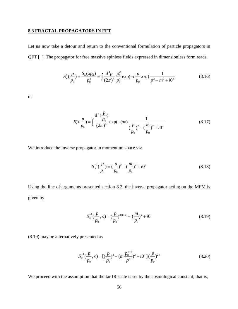
8.3 FRACTAL PROPAGATORS IN FFT

Let us now take a detour and return to the conventional formulation of particle propagators in

QFT [ ]. The propagator for free massive spinless fields expressed in dimensionless form reads

24

0 002 4 4 2 2

0 0 0 0

( ) 1( ) exp( )

(2 ) 0

bs

S xp pp d p pS i xp

p p p p p m i

(8.16)

or

4

0

42 20

0 0

( )1

( ) exp( )(2 )

( ) ( ) 0s

pd

ppS ipx

p mpi

p p

(8.17)

We introduce the inverse propagator in momentum space viz.

1 2 2

0 0 0

( ) ( ) ( ) 0s

p p mS i

p p p

(8.18)

Using the line of arguments presented section 8.2, the inverse propagator acting on the MFM is

given by

1 2(1 ) 2

0 0 0

( , ) ( ) ( ) 0s

p p mS i

p p p

(8.19)

(8.19) may be alternatively presented as

1

1 2 2 20

0 0 0

( , ) [( ) ( ) 0 ] ( )s

pp p pS m i

p p p p

(8.20)

We proceed with the assumption that the far IR scale is set by the cosmological constant, that is,

57

1

4IR ccp (8.21a)

Following [ ], dimensional regularization applied in the context of FFT requires the far IR scale

(1

4cc ), the electroweak scale ( )EWM and the far UV scale fixed by the Planck mass ( )UV PlM

to satisfy the constraint

14

( )cc EW

EW UV

MO

M

(8.21b)

We are now set to explore the IR region of field theory ranging from the electroweak scale

0 EWp M << UV to the far scale of cosmic distances EWM > p >>1

4cc . It makes sense to

revisit the arguments previously made, apply the formalism to the Higgs sector of the Standard

Model ( Hm m ) and cast (8.20) as

1

1 2 2 2( , ) [( ) ( ) 0 ]( )EWH H

EW EW EW

Mp p pS m i

M M p M

(8.22a)

Relation (8.22a) is well approximated by

1( , )HS P

≈ 2 2 2[ ( ) 0 ]HP M i P (8.22b)

where the “effective” momentum and “effective” Higgs mass are respectively defined as

EW

pP

M (8.23)

( )HH

EW

mM

p M (8.24)

58

A glance at (8.21a-b), (8.22a-b), and (8.5) reveals that the interpolating function

2( ) ( )

EW EW

p pf

M M

(8.25)

exhibits the following limiting behavior as << 1, ≠ 0

( ) ( )EW Hp O M O m 2( ) 1limEW

UV

M EW

p

M

(8.26)

p ≤ 1

4( )ccO << 1

4

2lim ( ) 0

cc

EW

EW

EW

M

pM

M

, if EW

pM

<< (8.27)

It is instructive to note here that, consistent with the principles of effective field theory, in the far

IR limit (8.27), the effective Higgs mass ( ( )HM ) of (8.22) diverges and naturally decouples

from physics occurring at very large distances.

Combined use of (8.25) and (8.27) yields

1 1 1

4 4 4

2 1 2lim '(0) lim 2 ( ) lim

( )cc cc cc

EW EW EW

EW

M M MEW

pf

pM

M

≈ 2

( )O

≈ (1)O (8.28)

provided that EW

pM

does not fall too far below . We shall use (8.22) and (8.26-28) in the next

section.

59

8.4 CLASSICAL GRAVITY AS LONG-RANGE EXCITATION OF THE HIGGS

CONDENSATE

An interesting proposal of [ ] is that classical gravity may be modeled as long-range and ultra-

weak excitation of the Higgs condensate. The approach developed here points in the same

direction: The MFM favors the onset of long-range coupling and the emergence of interpolating

functions of the type (8.4b) and (8.25) in the expression of propagators.

Following [ ], the connection between Newton’s constant ( )NG and Fermi’s constant ( )FG is

given by

2

24 '(0)

IRN F

H

pG G

f m (8.29)

Substituting (8.21a-b) and (8.28) in (8.29) leads to

NG ~ 3310 FG

(8.30)

in good agreement with currently known observational values of the two constants.

APPENDIX A

LIMITATIONS OF PERTURBATIVE RENORMALIZATION AND THE

CHALLENGES OF THE SM

In contrast with the paradigm of effective QFT (EFT), realistic RG flows approaching fixed

points are neither perturbative nor linear. We point out that overlooking these limitations is

necessarily linked to many unsolved puzzles challenging the SM. In particular, we show that the

60

analysis of non-linear attributes of RG flows near the electroweak scale can recover the full mass

and flavor structure of the SM. It is also shown that this analysis brings closure to the

“naturalness” puzzle without impacting the cluster decomposition principle of EFT.

1. INTRODUCTION

In his 1979 seminal paper on “Phenomenological Lagrangians” [ ], Steven Weinberg has

formulated the fundamental principles that any sensible EFT must comply with in order to

successfully explain the physics of the subatomic realm: QFT has no content besides unitarity,

analyticity, cluster decomposition and symmetries. This conjecture implies that, in order to

compute the S-matrix for any field theory below some scale, one must use the most general

effective Lagrangian consistent with these principles expressed in terms of the appropriate

asymptotic states [ ].

Closely related to Weinberg’s conjecture are two key aspects of EFT that deal with the

separation of heavy degrees of freedom from the light ones [ ]. One is the Decoupling Theorem

(Appelquist-Carrazone) stating that the effects of heavy particles go into local terms in a field

theory, either renormalizable couplings or in non-renomalizable effective interactions suppressed

by powers of the heavy scale. The other is Wilson’s Perturbative Renormalization Program [ ]

who teaches how to separate the degrees of freedom above and below a given scale and then to

integrate out all the high-energy effects and form a low-energy field theory with the remaining

degrees of freedom below the separation scale.

The idea of scale separation in EFT is typically illustrated by considering the perturbative

expansion of amplitudes in powers of momenta Q over a large scale UV , the latter setting the

upper limit of validity for the EFT [ ]

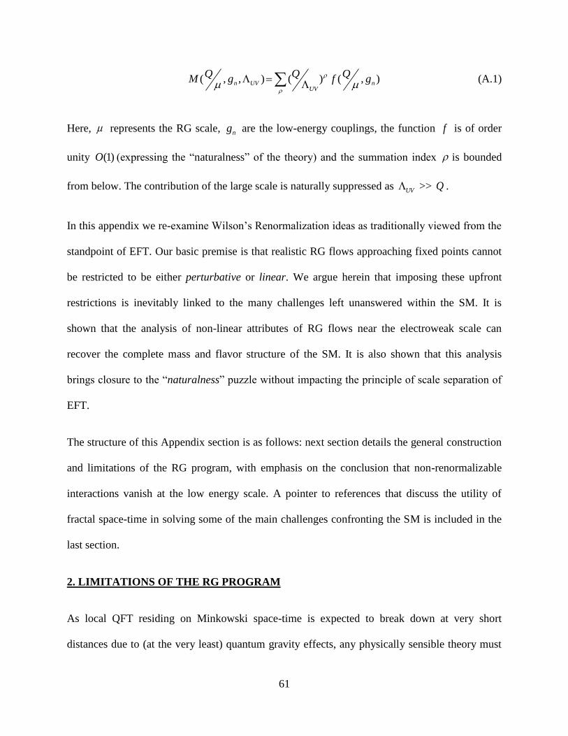
61

( , , ) ( ) ( , )n UV nUV

Q Q QM g f g

(A.1)

Here, represents the RG scale, ng are the low-energy couplings, the function f is of order

unity (1)O (expressing the “naturalness” of the theory) and the summation index is bounded

from below. The contribution of the large scale is naturally suppressed as UV >> Q .

In this appendix we re-examine Wilson’s Renormalization ideas as traditionally viewed from the

standpoint of EFT. Our basic premise is that realistic RG flows approaching fixed points cannot

be restricted to be either perturbative or linear. We argue herein that imposing these upfront

restrictions is inevitably linked to the many challenges left unanswered within the SM. It is

shown that the analysis of non-linear attributes of RG flows near the electroweak scale can

recover the complete mass and flavor structure of the SM. It is also shown that this analysis

brings closure to the “naturalness” puzzle without impacting the principle of scale separation of

EFT.

The structure of this Appendix section is as follows: next section details the general construction

and limitations of the RG program, with emphasis on the conclusion that non-renormalizable

interactions vanish at the low energy scale. A pointer to references that discuss the utility of

fractal space-time in solving some of the main challenges confronting the SM is included in the

last section.

2. LIMITATIONS OF THE RG PROGRAM

As local QFT residing on Minkowski space-time is expected to break down at very short

distances due to (at the very least) quantum gravity effects, any physically sensible theory must

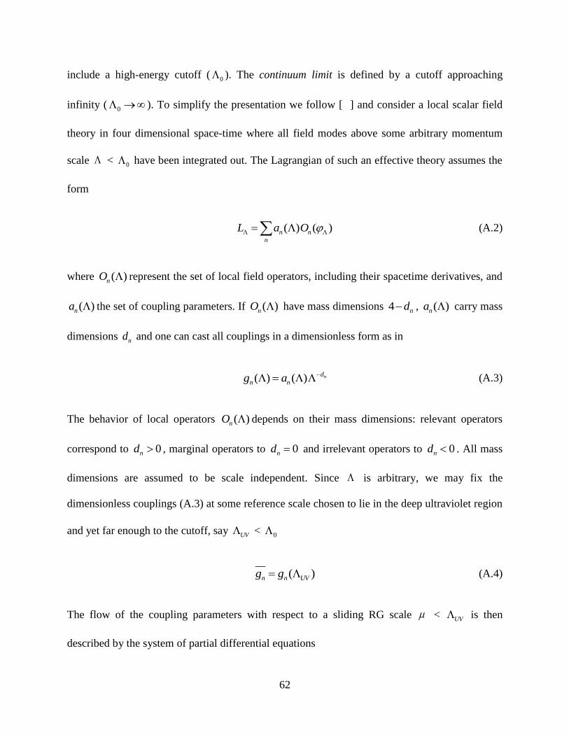
62

include a high-energy cutoff ( 0 ). The continuum limit is defined by a cutoff approaching

infinity ( 0 ). To simplify the presentation we follow [ ] and consider a local scalar field

theory in four dimensional space-time where all field modes above some arbitrary momentum

scale < 0 have been integrated out. The Lagrangian of such an effective theory assumes the

form

( ) ( )n n

n

L a O (A.2)

where ( )nO represent the set of local field operators, including their spacetime derivatives, and

( )na the set of coupling parameters. If ( )nO have mass dimensions 4 nd , ( )na carry mass

dimensions nd and one can cast all couplings in a dimensionless form as in

( ) ( ) nd

n ng a

(A.3)

The behavior of local operators ( )nO depends on their mass dimensions: relevant operators

correspond to 0nd , marginal operators to 0nd and irrelevant operators to 0nd . All mass

dimensions are assumed to be scale independent. Since is arbitrary, we may fix the

dimensionless couplings (A.3) at some reference scale chosen to lie in the deep ultraviolet region

and yet far enough to the cutoff, say UV < 0

( )n n UVg g (A.4)

The flow of the coupling parameters with respect to a sliding RG scale < UV is then

described by the system of partial differential equations

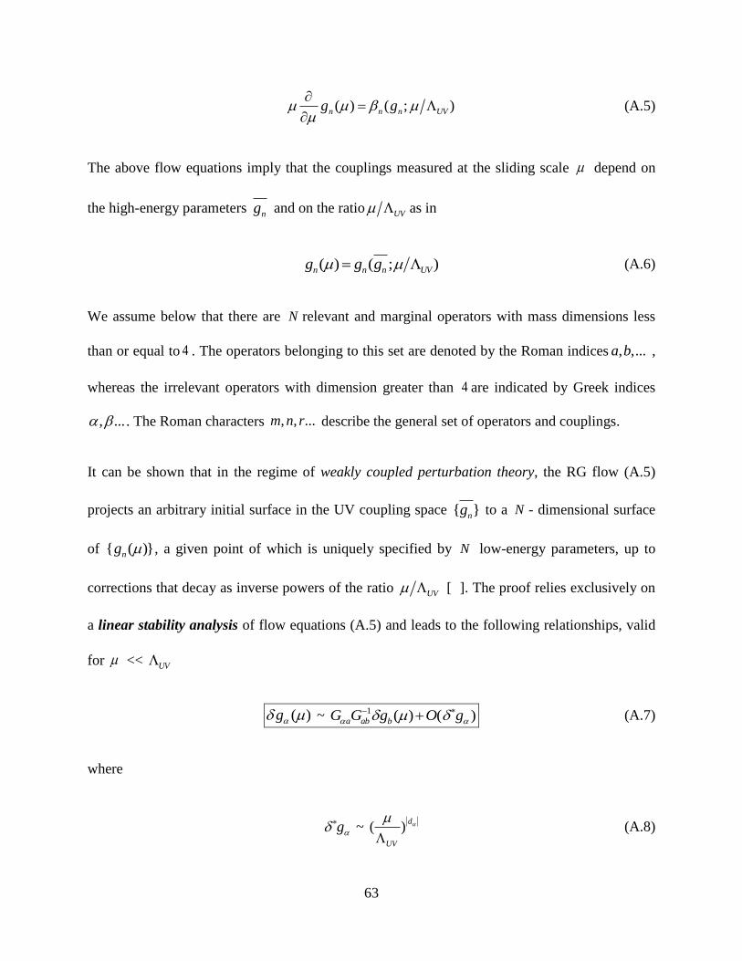
63

( ) ( ; )n n n UVg g

(A.5)

The above flow equations imply that the couplings measured at the sliding scale depend on

the high-energy parameters ng and on the ratio UV as in

( ) ( ; )n n n UVg g g (A.6)

We assume below that there are N relevant and marginal operators with mass dimensions less

than or equal to 4 . The operators belonging to this set are denoted by the Roman indices , ,...a b ,

whereas the irrelevant operators with dimension greater than 4 are indicated by Greek indices

, ... . The Roman characters , , ...m n r describe the general set of operators and couplings.

It can be shown that in the regime of weakly coupled perturbation theory, the RG flow (A.5)

projects an arbitrary initial surface in the UV coupling space { }ng to a N - dimensional surface

of { ( )}ng , a given point of which is uniquely specified by N low-energy parameters, up to

corrections that decay as inverse powers of the ratio UV [ ]. The proof relies exclusively on

a linear stability analysis of flow equations (A.5) and leads to the following relationships, valid

for << UV

( )g ~ 1 ( ) ( )a ab bG G g O g (A.7)

where

g ~ ( )d

UV

(A.8)

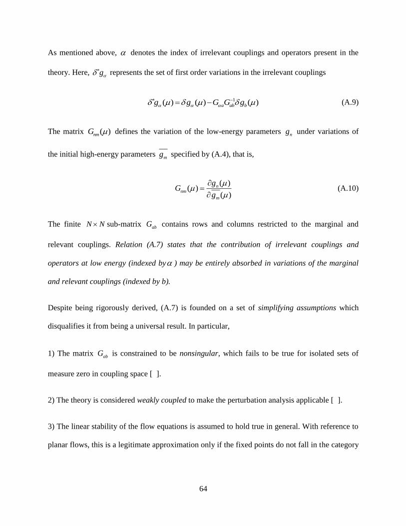
64

As mentioned above, denotes the index of irrelevant couplings and operators present in the

theory. Here, g represents the set of first order variations in the irrelevant couplings

1( ) ( ) ( )a ab bg g G G g (A.9)

The matrix ( )nmG defines the variation of the low-energy parameters ng under variations of

the initial high-energy parameters mg specified by (A.4), that is,

( )

( )( )

nnm

m

gG

g

(A.10)

The finite N N sub-matrix abG contains rows and columns restricted to the marginal and

relevant couplings. Relation (A.7) states that the contribution of irrelevant couplings and

operators at low energy (indexed by ) may be entirely absorbed in variations of the marginal

and relevant couplings (indexed by b).

Despite being rigorously derived, (A.7) is founded on a set of simplifying assumptions which

disqualifies it from being a universal result. In particular,

1) The matrix abG is constrained to be nonsingular, which fails to be true for isolated sets of

measure zero in coupling space [ ].

2) The theory is considered weakly coupled to make the perturbation analysis applicable [ ].

3) The linear stability of the flow equations is assumed to hold true in general. With reference to

planar flows, this is a legitimate approximation only if the fixed points do not fall in the category

65

of borderline equilibria (such as centers, degenerate nodes, stars or non-isolated attractors or

repellers) [ ]. Examples of such non-isolated fixed points are discussed in [ ].

4) The flow equations are assumed to correspond to Markov processes, that is, they are immune

to memory effects [ ].

5) Bound states are excluded from this approach, as they require an entirely non-perturbative

treatment [ ].

It is somehow surprising that many QFT textbooks do not explicitly point out the limitations that

these assumptions place on the validity of field theories in general. The widespread belief is that

they do not appear to directly impact the cluster decomposition principle and all SM predictions

up to the low-TeV scale probed by the LHC. However, in light of all unsettled questions

confronting the SM, one cannot help but wonder if some important piece of the puzzle is not lost

in overlooking these limitations. For example, over past decades the prevailing consequence of

the concept of “naturalness” for model building has been the cancellation of quadratic

divergences to the SM Higgs mass [ ]. According to this paradigm, the SM itself is an unnatural

theory, mandating new physics somewhere near the low-TeV scale. At the same time the LHC,

flavor physics, electroweak precision results and evaluation of the electron dipole moment all

point to the absence of any new phenomena in this range, which is however necessary to

accommodate the observation of both neutrino oscillations and cold Dark Matter [ ].

It seems that a paradigm shift is clearly needed to understand both the SM and the physics lying

beyond it. Tackling this challenge from a novel perspective on the RG program forms the topic

of the next section.

66

3. TOWARD A RESOLUTION OF SM CHALLENGES

Refs. [ ] describe how the concept of fractal space-time defined by 4D can be used to

bring closure to some of the main challenges left open by the SM.

We end this Appendix section with the key observation that, since the continuum field theory is

only an “effective” space-time model [ ], the effects induced by the dimensional parameter

4 D , with << 1 , are not perceivable in the computation of scattering amplitudes (A.1)

at the SM scale. With reference to (1.8) and (4.20), the condition << 1 is equivalent to setting

( )SM O Q << UV and the contribution of becomes strongly suppressed by the power

expansion (A.1). As a result, the cluster decomposition principle of EFT remains insensitive to

the emergence of fractal space-time near or above the SM scale ( ≥ SM ).

…ADDITIONAL APPENDIX SECTIONS AND REFERENCES TO FOLLOW…