Embed Size (px)
Citation preview
Low Carbon Manufacturing: Fundamentals,
Methodology and Application Case Studies
Sakda Tridech
A thesis submitted in partial fulfillment of the requirements of Brunel University
for the degree of Doctor of Philosophy
January 2012
Abstract
i
Abstract
The requirement and awareness of the carbon emissions reduction in several scales and
application of sustainable manufacturing have been now critically reviewed as important
manufacturing trends in the 21st century. The key requirements for carbon emissions reduction in
this context are energy efficiency, resource utilization, waste minimization and even the
reduction of total carbon footprint. The recent approaches tend to only analyse and evaluate
carbon emission contents of interested engineering systems. However, a systematic approach
based on strategic decision making has not been officially defined with no standards or
guidelines further formulated yet. The above requirements demand a fundamentally new
approach to future applications of sustainable low carbon manufacturing.
Energy and resource efficiencies and effectiveness based low carbon manufacturing (EREE-
based LCM) is thus proposed in this research. The proposed EREE-based LCM is able to provide
the systematic approach for integrating three key elements (energy efficiency, resource
utilization and waste minimization) and taking account of them comprehensively in a scientific
manner. The proposed approach demonstrates the solution for reducing carbon emissions in
manufacturing systems at both the machine and shop floor levels.
An integrated framework has been developed to demonstrate the feasible approach to achieve
effective EREE-based LCM at different manufacturing levels including machine, shop floor,
enterprise and supply chains. The framework is established in the matrix form with appropriate
tools and methodologies related to the three keys elements at each manufacturing level. The
theoretical model for EREE-based LCM is also presented, which consists of three essential
elements including carbon dioxide emissions evaluation, an optimization method and waste
reduction methodology. The preliminary experiment and simulations are carried out to evaluate
the proposed concept.
The modelling of EREE-based LCM has been developed for both the machine and shop floor
levels. At the machine level, the modelling consists of the simulation of energy consumption due
to the effect of machining set-up, the optimization model and waste minimization related to the
optimized machining set-up. The simulation is established using sugeno type fuzzy logic. The
learning method uses on experimental data (cutting trials) while the optimization model is

Abstract
ii
created using mamdani type fuzzy logic with grey relational grade technique. At the shop floor
level, the modelling is designed dependent on the cooperation with machine level modelling. The
determination of the work assignment including machining set-up depends on fuzzy integer
linear programming for several objectives with the evaluation of energy consumption data from
machine level modelling. The simulation method is applied as the part of shop floor level
modelling in order to maximize resource utilization and minimize undesired waste. The output
from the shop floor level modelling is machine production a planning with preventive plan that
can minimize the total carbon footprint.
The axiomatic design theory has been applied to generate the comprehensive conceptual model
E-R-W-C (energy, resource, waste and carbon footprint) of EREE-based LCM as a generic
perspective of the systematic modelling. The implementation of EREE-based LCM on both the
machine and shop floor levels are demonstrated using MATLAB toolbox and ProModel based
simulation. The proposed concept, framework and modelling have been further evaluated and
validated through case studies and experimental results.

Acknowledgements
iii
Acknowledgements
I would like to sincerely thank my PhD supervisor, Professor Kai Cheng, for his invaluable
support, guidance and encouragement throughout the programme of this research. Without his
support, the completion of the PhD project would not have been possible.
I would like to express my gratitude to The Royal Thai Government for its financial support
through the PhD scholarship, which has made this research possible. Special thanks also go to
my friends and colleagues, Dr. Xizhi Sun, Dr. Khalid Mohd Nor, Dr. Rasidi Ibrahim, Dr. Manida
Thongroon, Mr. Khir Harun, Mr. Paul Yates and other friends for their support and valuable
discussions throughout this research.
I would like to express my deep obligation to my parents, Dr. Saksit Tridech and Dr. Piyathida
Tridech. Even though, Dr. Saksit Tridech is now pass away, I still would like to give him the
most valuable credit for the encouragement from him. Thank you very much my beloved father.
I am also very graceful to Dr. Charnwit Tridech, my bigger brother and also my guardian in the
UK, for his assistance and encouragement.
Table of Contents
iv
Table of Contents
Abstract .......................................................................................................................................... i
Acknowledgements ..................................................................................................................... iii
Abbreviations ................................................................................................................................ x
Nomenclature .............................................................................................................................. xii
List of figures .............................................................................................................................. xiv
List of tables................................................................................................................................ xix
Chapter 1 Introduction.................................................................................................................. 1
1.1 Background of the research .................................................................................................... 1
1.1.1 Overview of the current carbon emission crisis .............................................................. 1
1.1.2 The current attempt carbon reduction in industrial sectors .............................................. 2
1.1.3 Trend and challenges for low carbon manufacturing in CNC based Manufacturing
systems ..................................................................................................................................... 6
1.2 Aims and objectives of the research ...................................................................................... 7
1.3 Structure of the thesis ............................................................................................................ 8
Chapter 2 Literature Review ..................................................................................................... 10
2.1 Introduction ......................................................................................................................... 10
2.2 State of the art of sustainable manufacturing ...................................................................... 10
2.2.1 Current research areas in the sustainable manufacturing ............................................. 11
2.2.1.1 The role of operational model on environmental management ............................ 11
2.2.1.2 Waste reduction using lean manufacturing ........................................................... 12
Table of Contents
v
2.2.1.3 Environmental issues on machining systems ........................................................ 14
2.2.1.4 Strategic and planning for sustainable manufacturing .......................................... 17
2.2.1.5 The utilization of renewable energy ..................................................................... 19
2.3 Low carbon manufacturing ................................................................................................. 23
2.3.1 Characteristic of low carbon manufacturing ................................................................ 23
2.3.2 The initial design for low carbon manufacturing system ............................................. 27
2.4 Multi-criteria decision making techniques .......................................................................... 29
2.4.1 Analytical Hierarchy Process (AHP) ............................................................................ 29
2.4.2 Fuzzy Logic .................................................................................................................. 31
2.4.3 Taguchi method ............................................................................................................ 32
2.5 Flexible manufacturing ....................................................................................................... 35
2.6 Axiomatic design ................................................................................................................. 38
2.7 Summary ............................................................................................................................. 41
Chapter 3 Research Methodologies ........................................................................................... 42
3.1 Introduction ......................................................................................................................... 42
3.2 The scope of research methodology .................................................................................... 42
3.3 The experimental set-up ...................................................................................................... 44
3.3.1 CNC milling machine ................................................................................................... 44
3.3.2 Data acquisition of electrical energy ............................................................................ 46
3.4 Software tools ...................................................................................................................... 49
3.4.1 Fuzzy logic toolbox ...................................................................................................... 49
Table of Contents
vi
3.4.2 ProModel ...................................................................................................................... 50
3.4.3 Genetic Algorithm toolbox on MATLAB based .......................................................... 53
3.5 Summary ............................................................................................................................. 55
Chapter 4 A Framework for Developing EREE-based LCM ................................................. 57
4.1 Summary ............................................................................................................................. 57
4.2 State of the art ..................................................................................................................... 57
4.2.1 Carbon emission analysis ............................................................................................. 59
4.2.2 Operational model ........................................................................................................ 60
4.2.3 Desktop and micro factory ........................................................................................... 60
4.2.4 The novell approach: devolved manufacturing ............................................................ 61
4.3 Characterization of low carbon manufacturing ................................................................... 61
4.4 EREE-based LCM: conception and a framework ............................................................... 63
4.5 LCM theoretical model ....................................................................................................... 67
4.6 Implementation of LCM at enterprise and supply chain level ............................................ 71
4.7 Implementation of LCM at machine and shop-floor level .................................................. 73
4.8 Modeling of carbon footprint in EREE-based LCM ........................................................... 75
4.8.1 Machine/process energy consumption ......................................................................... 75
4.8.2 Resource utilization ...................................................................................................... 76
4.8.3 Waste minimization ...................................................................................................... 76
4.9 Operational models for LCM .............................................................................................. 77
4.9.1 An operational model at supply chain level ................................................................. 77
Table of Contents
vii
4.9.2 An operational model at shop-floor level ..................................................................... 79
4.10 Experiments and results ..................................................................................................... 80
4.10.1 The system and process .............................................................................................. 80
4.10.2 Optimization procedures ............................................................................................ 81
4.10.3 Results ........................................................................................................................ 82
4.10.4 Carbon emissions ........................................................................................................ 83
4.11 Summary ........................................................................................................................... 84
Chapter 5 Modeling of EREE-based LCM .............................................................................. 85
5.1 Introduction ......................................................................................................................... 85
5.2 The scope and boundary of developing a system approach for low carbon manufacturing
.................................................................................................................................................... 85
5.3 The conceptual model for EREE-based low carbon manufacturing ................................... 88
5.4 Transformation of conceptual design into logical approach ............................................... 91
5.4.1 Energy efficiency .......................................................................................................... 91
5.4.2 Resource utilization ...................................................................................................... 94
5.4.3 Waste minimization .................................................................................................... 100
5.5 The systematic approach for applying the conceptual model to achieve LCM ................ 103
5.6 EREE-based LCM at machine level .................................................................................. 106
5.6.1 The cutting force system ............................................................................................ 106
5.6.1.1 Cutting force model ............................................................................................ 107
5.6.1.2 Chip load model .................................................................................................. 108
Table of Contents
viii
5.6.2 Energy consumption model for the conventional motor ............................................ 109
5.6.3 Modelling and application for machine level ............................................................. 113
5.6.4 Environment of EREE-based LCM for energy efficiency and resource
optimization ......................................................................................................................... 122
5.7 Preparation of waste .......................................................................................................... 127
5.8 Implementation of waste minimization at the machine level ............................................ 128
5.9 EREE-based LCM at shop-floor level .............................................................................. 132
5.9.1 Modelling and application for shop-floor level .......................................................... 132
5.9.2 The proposed concept for development of optimization model at shop-
floor level ............................................................................................................................. 133
5.9.3 Optimization method .................................................................................................. 136
5.9.4 Optimization model .................................................................................................... 138
5.9.5 Simulation model for waste elimination ..................................................................... 140
5.9.5.1 The application of waste elimination model ....................................................... 141
5.10 Summary ......................................................................................................................... 145
Chapter 6 Application Case Studies and Discussions ............................................................ 146
6.1 Introduction ....................................................................................................................... 146
6.2 EREE-based LCM case study one ..................................................................................... 146
6.2.1 Experimental set-up ............................................................................................... 146
6.2.2 Design of experiments ........................................................................................... 148
6.2.3 Experiments and results ......................................................................................... 151
6.2.4 Establishment of energy prediction model ............................................................ 153
Table of Contents
ix
6.2.5 Prediction and optimization of machining parameters for energy efficiency
and cost effective ............................................................................................................ 155
6.2.6 Optimization of machining parameters using grey-fuzzy logic based ................... 157
6.2.7 Analysis of energy efficiency and carbon footprint ............................................... 163
6.3 EREE-based LCM case study two .................................................................................... 165
6.3.1 Simulation model for maximization of resource utilization and waste
minimization ................................................................................................................... 165
6.3.2 Numerical example and results .............................................................................. 167
6.4 Summary ........................................................................................................................... 176
Chapter 7 Conclusions and Recommendations for Future Work ........................................ 177
7.1 Conclusions ....................................................................................................................... 177
7.2 Contributions to knowledge .............................................................................................. 178
7.3 Recommendations for future work .................................................................................... 179
References .................................................................................................................................. 180
Appendices I A list of publications resulted from the research ............................................ 197
Appendices II Parts of programmes of machining with energy efficiency .......................... 199
Appendices III Parts of programmes using to establish model in ProModel ....................... 207
Abbreviations
x
Abbreviations
AHP Analytical Hierarchy Process
AI Artifact Intelligent
ANFIS Neuro Fuzzy Inference Systems
BOM Bill of Materials
BSI The British Standard
CFCs Chlorofluorocarbons
CH4 Methane
CHP Combined Heat and Power
CNC Computer Numerical Control
CO2 Carbon Dioxide
DM Devolved Manufacturing
EIO Enterprise Input-Output Model
EREE Energy Resource Efficiency and Effectiveness
ERP Enterprise Resource Planning
FIS Fuzzy Inference System
FMS Flexible Manufacturing
GA Genetic Algorithm
GDP Gross Domestic Product
GHG Greenhouse Gas
GUI Graphical User Interface
IPCC Intergovernmental Panel on Climate Change
ISO International Organization for Standardization
JIT Just In Time
LCA Life Cycle Assessment
Abbreviations
xi
LCM Low Carbon Manufacturing
LP Linear Programming Solution
MADM Multi-Attribute Decision Making
MC Mass Customization
MCDM Multi-Criteria Decision Making
MODM Multi-Objective Decision Making
MPS Master Production Planning
MRR Material Removal Rate
N2O Nitrous Oxide
OA Orthogonal Array
OR Operations Research
PMPP Poss Mass Production Paradigm
RSM Response Surface Methodology
Nomenclature
xii
Nomenclature
Cijk set-up cost for operation j of workpiece i performing on machine k
Eijk energy consumption using for operation j of workpiece i performing on machine k
ft the feed per tooth (mm)
F force (N)
I current (amp)
m machine type; Mm ,...,2,1∈
Nf number of teeth
Ns spindle speed (RPM)
o operation for workpiece w; Owo ,...,2,1∈
P power (watt or hp)
R distance (m)
RPM rotational speed
Smw set of workpiece can perform on machine m
Sow set of operation of workpiece can perform on machine m
Swo set of machine can perform operation o of workpiece w
T time (sec)
Tijk production time used for operation j of workpiece i performing on machine k
V voltage (volt)
Vf feed rate (mm/minute)
w workpiece type; Ww ,...,2,1∈

Nomenclature
xiii
W work (N·m)
Xijk operation j of workpiece i performing on machine k
angle of the wave form
angular speed (ω)
function of total energy consumption
function of total cost of operation
function of total production time
torque (N·m)
List of Figures
xiv
List of Figures
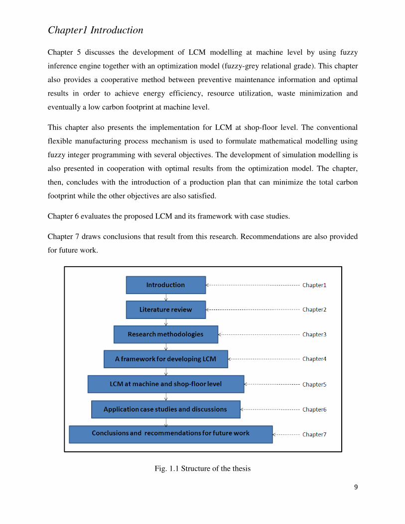
Fig. 1.1 Structure of the thesis ......................................................................................................... 9
Fig. 2.1 A JIT factory design ........................................................................................................ 13
Fig. 2.2 Reconfigurable machines ................................................................................................ 14
Fig. 2.3 Conventional machining process ..................................................................................... 15
Fig. 2.4 The environment of manufacturing process .................................................................... 17
Fig. 2.5 The conventional life cycle .............................................................................................. 19
Fig. 2.6 The EIO model ................................................................................................................ 19
Fig. 2.7 The utilization of source of renewable energy ................................................................ 21
Fig. 2.8 The logical of energy supply for bio-energy ................................................................... 23
Fig. 2.9 The conceptual model for zero carbon manufacturing .................................................... 25
Fig. 2.10 Process for developing an embedded GHG database emissions ................................... 26
Fig. 2.11 Process of the low carbon product design system ......................................................... 26
Fig. 2.12 The evaluation system for energy efficiency ................................................................. 27
Fig. 2.13 Energy and materials inputs and outputs of manufacturing process ............................. 28
Fig. 2.14 Product life cycle based on EU-LCA platform ............................................................. 28
Fig. 2.15 The example of carbon footprint calculation using PAS2050 ........................................ 28
Fig. 2.16 The example of hierarchy structure using AHP method ............................................... 30
Fig. 2.17 Fuzzy inference system ................................................................................................. 31
Fig. 2.18 Main effect plot using MINITAB .................................................................................. 34
Fig. 2.19 UK electricity demand by sector 2008 ........................................................................... 37
List of Figures
xv
Fig. 2.20 The diagram of typical CNC machine ........................................................................... 37
Fig. 2.21 The comparison between different machine set-up ....................................................... 38
Fig. 2.22 Four domains in Axiomatic Design ............................................................................... 39
Fig. 2.23 Zigzagging in Axiomatic Design ................................................................................... 40
Fig. 3.1 The scope of research methodology ................................................................................ 43
Fig. 3.2 Breidgeport CNC milling machine .................................................................................. 44
Fig. 3.3 Three phase power supply of Bridgeport ........................................................................ 45
Fig. 3.4 Snapshot of CNC milling machine of Thailand laboratory ............................................. 46
Fig. 3.5 ISO-TECH IPM 3005 ....................................................................................................... 47
Fig. 3.6 Connection method of the device to power supply ......................................................... 47
Fig. 3.7 Setup of Primus PC-02 ..................................................................................................... 48
Fig. 3.8 Fuzzy logic toolbox on MATLAB based ........................................................................ 50
Fig. 3.9 The relation between event and FIS GUI ........................................................................ 50
Fig. 3.10 The time weight simulation result using ProModel ....................................................... 51
Fig. 3.11 Environments in the model ............................................................................................ 52
Fig. 3.12 Processing editor in ProModel ...................................................................................... 52
Fig. 3.13 Objective establishment in M-file ................................................................................. 54
Fig. 3.14 Constraint establishment in M-file ................................................................................ 55
Fig. 3.15 Running GA from command line .................................................................................. 55
Fig. 4.1 Characterization of Low Carbon Manufacturing ............................................................. 61
Fig. 4.2 The conception and outcome of EREE-based LCM ....................................................... 64
List of Figures
xvi
Fig. 4.3 The theoretical model of LCM ........................................................................................ 68
Fig. 4.4 Implemented Concepts for LCM ..................................................................................... 72
Fig. 4.5 Energy measurement ....................................................................................................... 74
Fig. 4.6 Energy modelling ............................................................................................................ 74
Fig. 4.7 Resource utilization ......................................................................................................... 74
Fig. 4.8 Discrete simulations in ProModel ................................................................................... 74
Fig. 4.9 Modelling of carbon footprint in EREE-based LCM ...................................................... 75
Fig. 4.10 The concept of the capacitated flow model for low carbon manufacturing .................. 77
Fig. 4.11 The configuration of the systems in ProModel simulations .......................................... 82
Fig. 4.12 Location states single of the first system ....................................................................... 82
Fig. 4.13 Location states single of the second system .................................................................. 83
Fig. 4.14 The status of Motor1 in the first (left) system and second (right) system ..................... 83
Fig 5.1 The causes of carbon footprint in FMS ............................................................................ 88
Fig. 5.2 Transformation of design parameter into logical approach ............................................. 91
Fig. 5.3 Procedure at energy efficiency stage ............................................................................... 92
Fig. 5.4 The transformation of generic model into mathematical method .................................... 96
Fig. 5.5 Simulation model for waste minimization ..................................................................... 101
Fig. 5.6 Applied conceptual model for systematic approach ...................................................... 104
Fig. 5.7 The conventional dynamic end milling cutting force prediction model ........................ 107
Fig. 5.8 The elemental cutting forces applied to a flute on the end mill .................................... 108
Fig. 5.9 The thickness of chip load formation ............................................................................ 109
List of Figures
xvii
Fig. 5.10 The configuration of conventional AC motor ............................................................. 110
Fig. 5.11 Cutting trial using 2500 rpm, 1000 mm/min and 1 mm .............................................. 112
Fig. 5.12 Cutting trial using 4166 rpm, 1666.4 mm/min and 1 mm ........................................... 113
Fig. 5.13: EREE-based LCM for machine level ......................................................................... 115
Fig. 5.14 EREE model at machine level performing on aluminum cutting trial ........................ 115
Fig. 5.15 The drawing layout of all cutting trials on the aluminum plate ................................... 118
Fig. 5.16 The user interface for the measurement device ........................................................... 118
Fig. 5.17 Energy consumption using 400 SFM, 12 Ømm, 1mm ................................................ 120
Fig. 5.18 Energy consumption using 500 SFM, 12 Ømm, 2mm ................................................ 121
Fig. 5.19 Architecture of the optimization system ...................................................................... 123
Fig. 5.20 The overall of system perspectives .............................................................................. 123
Fig. 5.21 The main interface of the energy efficiency and optimization system ........................ 125
Fig. 5.22 Machining parameters input interface ......................................................................... 125
Fig. 5.23 Costs preparation input interface ................................................................................. 126
Fig. 5.24 The evaluation and optimization results ...................................................................... 127
Fig. 5.25 Preparation of waste occurrence .................................................................................. 128
Fig. 5.26 The model layout of waste minimization at the machine level ................................... 129
Fig. 5.27 Time weight value of machine down time .................................................................. 131
Fig. 5.28 EREE-based model for shop-floor level ...................................................................... 133
Fig. 5.29 Simulation model for waste energy elimination .......................................................... 141
Fig. 5.30 Simulation model for waste elimination ...................................................................... 142
List of Figures
xviii
Fig. 6.1 The connection of the measurement device with the CNC machine ............................. 147
Fig. 6.2 The full experiment set-up ............................................................................................. 147
Fig. 6.3 workpiece(1)@ 2500rpm:1000mm/min:1mm ............................................................... 151
Fig. 6.4 Workpiece(2)@ 4166rpm:1666.4mm/min:1mm ........................................................... 152
Fig. 6.5 The final membership function of SFM, tool size and depth of cut .............................. 154
Fig. 6.6 Membership function for grey relational coefficient of energy consumption and costs
preparation .................................................................................................................................. 158
Fig. 6.7 Membership function for evaluating fuzzy reasoning grade ......................................... 158
Fig. 6.8 Fuzzy rules using in the mamdani type FIS .................................................................. 159
Fig. 6.9 The effect of machine parameters on considered response using FIS
based…………............................................................................................................................161
Fig. 6.10 The effect of machine parameters on considered response using RSM
based………................................................................................................................................163
Fig. 6.14 Energy consumption and carbon footprint from each scenario ................................... 164
Fig. 6.15 FMS simulation model for waste minimization .......................................................... 166
Fig. 6.16 Carbon footprint occurred from each scenario ............................................................ 173
List of Tables
xix
xix
List of Tables
Table 1.1 Electricity consumption trends 2005-2008 ............................................................................ 3
Table 1.2 Gas consumption trends 2005-2008 ....................................................................................... 3
Table 1.3 Emissions limitation proposals for European countries (IPCC) ......................................... 4
Table 1.4 Emissions limitation proposals for European countries: 2000-2100 (IPCC) .................... 4
Table 1.5 Emissions factors from IPCC .................................................................................................. 5
Table 2.1 Energy analysis on commercial machines ........................................................................... 16
Table 2.2 Energy consumption using in iron and steel manufacturing of UK industry…………16
Table 2.3 Fuzzy reasoning grade related to each experiment32 ........................................................ 34
Table 2.4 Response of parameter on the response ............................................................................... 35
Table 3.1 Specifications of the Bridgeport machine ............................................................................ 44
Table 3.2 Specifications of the CNC milling machine ........................................................................ 45
Table 3.3 The specification of ISO-TECH IPM 3005 ......................................................................... 48
Table 3.4 The specifications of Primus PC-02 ..................................................................................... 48
Table 4.1 Modelling efforts in EREE-related manufacturing research ............................................. 58
Table 4.2 The characterization of EREE-based low carbon manufacturing .................................... 64
Table 4.3 Processing time of the gear and spindle on each machine ................................................ 80
Table 4.4 Energy consumption rate to produce the product on each machine ................................. 80
Table 4.5 Oil consumption rate to produce the product on each machine ........................................ 81
Table 4.6 Operational shift for each device……………………………………………………...81
Table 4.7 Carbon emissions from the first and second system .......................................................... 84
List of Tables
xx
Table 5.1 Experimental results of cutting trial............................................................................... 93
Table 5.2 The decision matrix of process condition at machine level ........................................... 97
Table 5.3 The data of energy consumption and cost of preparation .............................................. 98
Table 5.4 The primary information obtained from the evaluation model...................................... 99
Table 5.5 Simulation of waste during the process using discrete event simulation .................... 102
Table 5.6 Parameters used in cutting trials for recording energy consumption ........................... 118
Table 5.7 The variation in energy consumption from different machining set-up ...................... 120
Table 5.8 Simulation results from fuzzy logic and RSM comparing with
experimental results ..................................................................................................................... 122
Table 5.9 Parameters for simulation set-up ................................................................................. 130
Table 5.10 Percentage of machine down time ............................................................................ 130
Table 5.11 Percentage of resource utilization .............................................................................. 131
Table 5.12 The conventional job-shop with machining optimization ........................................ 134
Table 5.13 Optimal machining set-up for shop-floor level provided by machine
level modeling .............................................................................................................................. 135
Table 5.14 Energy consumption (kWh) for machining the workpiece ........................................ 136
Table 5.15 Wastes occurring from manufacturing process ......................................................... 143
Table 5.16 Input parameter of waste elimination model ............................................................. 143
Table 5.17 Preventive plan obtaining from simulation results .................................................... 144
Table 5.18 Simulation results using preventive plan ................................................................... 144
Table 6.1 The selected cutting parameters associated with their levels ...................................... 148
List of Tables
xxi
Table 6.2 The combination of selected parameters for each cutting trial ................................... 149
Table 6.3 The conventional machining parameters for all cutting sequences ............................. 150
Table 6.4 The energy consumption results from 24 cutting trials .............................................. 152
Table 6.5 Input parameters for both systems ............................................................................... 155
Table 6.6 the L9 orthogonal array of taguchi method ................................................................ 155
Table 6.7 Evaluated results using defuzzification and response surface .................................... 156
Table 6.8 Data preprocessing and grey relational coefficient from FIS and RSM ...................... 157
Table 6.9 The grey-fuzzy reasoning grade from FIS and RSM ................................................... 159
Table 6.10 Calculation of effect from machining parameters using FIS based ........................... 160
Table 6.11 Response table for the grey-fuzzy reasoning grade using FIS based ........................ 161
Table 6.12 Calculation of effect from machining parameters using RSM based ........................ 162
Table 6.13 Response table for the grey-fuzzy reasoning grade using RSM based ...................... 163
Table 6.14 The energy consumption for selected scenario .......................................................... 164
Table 6.15 Type of waste occurred from each machine after simulation .................................... 166
Table 6.16 Parameters used in the simulation model for the considered case study ................... 167
Table 6.17 Energy consumption (kWh) for machining the workpiece ........................................ 168
Table 6.18 Costs of production (£) for machining the workpiece ............................................... 168
Table 6.19 Production time (min) for machining the workpiece ................................................. 169
Table 6.20 Optimal set-up for machine operation ....................................................................... 169
Table 6.21 Scenarios of optimized results ................................................................................... 170
Table 6.22 Hidden waste (carbon footprint) from each scenario after simulation applied .......... 173

List of Tables
xxii
Table 6.23 The operational strategy applied to each scenario to reduce waste at
shop-floor level ............................................................................................................................ 174
Table 6.24 Simulation results without proposed model ............................................................... 175
Table 6.25 Simulation results with proposed model .................................................................... 175
Chapter1 Introduction
1
Chapter 1 Introduction
1.1 Background of the research
1.1.1 Overview of the current carbon emissions crisis
Greenhouse gas
A greenhouse gas (GHG) is normally referred to as a gas in the atmosphere layer that absorbs
and emits radiation within the thermal infrared range. This process is fundamental to the
“greenhouse gas effect” (Pepper 2006). Typically, the primary greenhouse gases include carbon
dioxide (CO2), nitrous oxide (N2O), chlorofluorocarbons (CFCs), methane (CH4) and
tropospheric ozone. From 1899 to 1960, many researchers believed that the effect of greenhouse
gas could be beneficial and neutral to human kind due to the effect of the warming temperature
on the world’s atmosphere. The major advantage from this effect was to prevent the beginning of
the new ice age in the future. However, many researchers critically noticed that the large scale of
geophysical resources that can’t be reproduced or renewable is crucially affected by the
exponential growth of the human population. With this clue, researchers have determined that
the effects of greenhouse gas are a harmful factor for the ecosystem and society (Trenberth
1995).
Source of carbon dioxide (CO2)
The rise in carbon dioxide emissions is now considered as the main effect on the global warming
problem from the greenhouse gas. The amount of carbon dioxide emissions has approximately
increased by 25% since the beginning of the industrial revolution in the early eighteenth century.
CO2 is normally emitted from the industrial process by burning fossil fuels. Fossil fuels are
commonly used for electric power generation, transportation, heating and cooling processes and
in manufacturing. The burning of coal and wood also emits CO2. Taking the current situation
into account, it is expected that developing countries will emit greenhouse gases at the same
level or even higher than the emissions levels of developed countries as a result of the rise in
energy and food demand associated with the increase in the human population (Trenberth 1995).
Chapter1 Introduction
2
1.1.2 The current attempt at carbon reduction in industrial sectors
Today, the increase in carbon dioxide (CO2) emissions is becoming the crucial factor in the
global warming problem, especially in industrial sectors. As the main source of carbon
emissions, all types of energy transformed from fossil fuels play the most important role in this
critical problem (Kone A. C. 2010). The environmental impacts at the local, national and global
levels have been rising as the population increases, which leads to more energy consumption.
With this information, it can be implied that the reduction plan of carbon emissions using purely
policy based approaches might not be enough at the present. In the industrial sector, it was
reported that the industrialised and developing countries have the greatest responsibility to take
action on the reduction of carbon emissions according to the Kyoto Protocol (Omer 2008). The
agreement and framework in the Kyoto Protocol, it significantly states that developed countries
must decrease their total emissions of green house gas (GHG) by at least 5% based on 1990
levels. This action has to be taken during 2008-2012 (Mirasgedis 2002; Erdogdu 2010). As
different sectors have become aware of the negative outcomes from this problem, many
researchers have begun to develop solutions in the forms of methodology and innovation such as
renewable energy planning, energy resource allocation, transportation energy management or
electric utility planning (Pohekar 2004). Therefore, it is essential to develop a systematic
approach for Low Carbon Manufacturing (LCM), which is related to the manufacturing process
that produces low carbon emissions and uses energy and resources efficiently and effectively
during the process (Tridech 2008).
In relation to sustainability problems, many manufacturers have been suffering the crucial effect
of resources and supplies being changed, especially in terms of energy and raw materials. For
instance, energy prices and demand have rapidly increased and oil production is predicted to
intensively produce to reach its maximum capacity due to the higher level of demand compared
to the supply level. In addition, in the case of materials, the consumption rate and price of steel
have doubled in the last decade and the demand is also expected to surpass the supply level as
well as oil production. As a result of this crisis, the introduction of a carbon trading system such
as the EU Emission Trading Scheme regarding the requirement of carbon footprint reduction and
manufacturing cost effectiveness is now a high priority to be considered (Mehling 2009).
Chapter1 Introduction
3
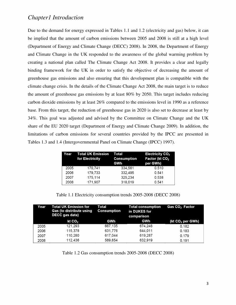
Due to the demand for energy expressed in Tables 1.1 and 1.2 (electricity and gas) below, it can
be implied that the amount of carbon emissions between 2005 and 2008 is still at a high level
(Department of Energy and Climate Change (DECC) 2008). In 2008, the Department of Energy
and Climate Change in the UK responded to the awareness of the global warming problem by
creating a national plan called The Climate Change Act 2008. It provides a clear and legally
binding framework for the UK in order to satisfy the objective of decreasing the amount of
greenhouse gas emissions and also ensuring that this development plan is compatible with the
climate change crisis. In the details of the Climate Change Act 2008, the main target is to reduce
the amount of greenhouse gas emissions by at least 80% by 2050. This target includes reducing
carbon dioxide emissions by at least 26% compared to the emissions level in 1990 as a reference
base. From this target, the reduction of greenhouse gas in 2020 is also set to decrease at least by
34%. This goal was adjusted and advised by the Committee on Climate Change and the UK
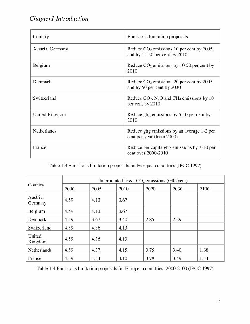
share of the EU 2020 target (Department of Energy and Climate Change 2009). In addition, the
limitations of carbon emissions for several countries provided by the IPCC are presented in
Tables 1.3 and 1.4 (Intergovernmental Panel on Climate Change (IPCC) 1997).
Table 1.1 Electricity consumption trends 2005-2008 (DECC 2008)
Table 1.2 Gas consumption trends 2005-2008 (DECC 2008)
Chapter1 Introduction
4
Country Emissions limitation proposals
Austria, Germany Reduce CO2 emissions 10 per cent by 2005, and by 15-20 per cent by 2010
Belgium Reduce CO2 emissions by 10-20 per cent by 2010
Denmark Reduce CO2 emissions 20 per cent by 2005, and by 50 per cent by 2030
Switzerland Reduce CO2, N2O and CH4 emissions by 10 per cent by 2010
United Kingdom Reduce ghg emissions by 5-10 per cent by 2010
Netherlands Reduce ghg emissions by an average 1-2 per cent per year (from 2000)
France Reduce per capita ghg emissions by 7-10 per cent over 2000-2010
Table 1.3 Emissions limitation proposals for European countries (IPCC 1997)
Country Interpolated fossil CO2 emissions (GtC/year)
2000 2005 2010 2020 2030 2100
Austria, Germany
4.59 4.13 3.67
Belgium 4.59 4.13 3.67
Denmark 4.59 3.67 3.40 2.85 2.29
Switzerland 4.59 4.36 4.13
United Kingdom
4.59 4.36 4.13
Netherlands 4.59 4.37 4.15 3.75 3.40 1.68
France 4.59 4.34 4.10 3.79 3.49 1.34
Table 1.4 Emissions limitation proposals for European countries: 2000-2100 (IPCC 1997)
Chapter1 Introduction
5
For the initial step of achieving low carbon manufacturing, there are now two methodologies
being broadly applied: carbon footprint assessment (by multiplying emission factor with
consumed energy) and an introduction for a low carbon industrial strategy(Intergovernmental
Panel on Climate Change (IPCC) 2006; Department of Energy and Climate Change (DECC)
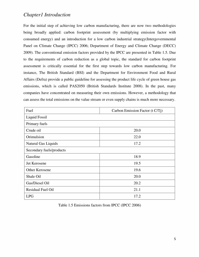
2009). The conventional emission factors provided by the IPCC are presented in Table 1.5. Due
to the requirements of carbon reduction as a global topic, the standard for carbon footprint
assessment is critically essential for the first step towards low carbon manufacturing. For
instance, The British Standard (BSI) and the Department for Environment Food and Rural
Affairs (Defra) provide a public guideline for assessing the product life cycle of green house gas
emissions, which is called PAS2050 (British Standards Institute 2008). In the past, many
companies have concentrated on measuring their own emissions. However, a methodology that
can assess the total emissions on the value stream or even supply chains is much more necessary.
Fuel Carbon Emission Factor (t C/Tj)
Liquid Fossil
Primary fuels
Crude oil 20.0
Orimulsion 22.0
Natural Gas Liquids 17.2
Secondary fuels/products
Gasoline 18.9
Jet Kerosene 19.5
Other Kerosene 19.6
Shale Oil 20.0
Gas/Diesel Oil 20.2
Residual Fuel Oil 21.1
LPG 17.2
Table 1.5 Emissions factors from IPCC (IPCC 2006)
Chapter1 Introduction
6
Although carbon footprint evaluation is now available as an official guideline, the systematic
methodology that can achieve energy efficiency and effectiveness and eventually lower carbon
footprints has not been made available yet, despite the fact that this issue has been discussed as a
timely topic in order to find out the scientific manner. For instance, the Department of Business,
Enterprise and Regulatory Reform and the Department of Energy and Climate Change in the UK
recently introduced a pilot campaign called “Low Carbon Industrial Strategy: A Vision” to
inspire enterprises to create a low carbon economy (Department for Business Enterprise and
Regulatory Reform and Department of Energy and Climate Change 2009). This guideline
specifically suggests the important four drivers to create a Low Carbon Industry:
(1) Achieving energy efficiency to save businesses, consumers and the public services
money
(2) Encouragement in critical factors for the UK’s low carbon industry platform such
as renewable energy, nuclear power, Carbon Capture and Storage and a ‘smart’
grid
(3) Applying low carbon industry concepts to the future UK automotive industry
(4) Providing support for research and development, human skills and demonstration
for every business area
1.1.3 Trends and challenges for low carbon manufacturing in CNC based manufacturing systems
Nowadays, the term of mass customization can be referred to as the capability that can generate
goods and services at a high production rate. This technology can also give manufacturers the
ability to customize product specifications due to customer needs (Slack, 2004). This includes
Internet based manufacturing, which can remotely control output and customization. Logically,
consumers normally expect the outputs/products that can precisely fulfill their requirements and
even have valuable manufacturing features of quality that is produced on time and for the right
costs. Hence, many manufacturers have suffered the impact of the current manufacturing
platform that has moved forward to the new suitable technologies and processes to gain high
value manufacturing.
However, the future trend of world manufacturing cannot just rely on conventional
manufacturing performance due to the emergence of the sustainable development concept and
Chapter1 Introduction
7
even the national crisis of carbon dioxide reduction. From this point of view, it is very essential
for current products and services to be integrated with the characterizations of the sustainable
principle (Jovane 2008). Thus, manufacturers must address environmental issues together with
conventional manufacturing performance and also prepare new methodologies and innovations
to cope with the future manufacturing demand of society (Byrne 1993).
And yet, the existing low carbon manufacturing for CNC based manufacturing systems and even
generic modelling are not systematically formulated. Even though, renewable energy, alternative
fuels and new innovation devices for energy have been rapidly developed to solve the global
warming problem and fulfill sustainable development, the methodologies and processes that can
improve and transform the existing system to a low carbon industry are not available at this
moment. In CNC based manufacturing, there are many variables and factors that can affect the
total energy consumption and eventually total carbon emissions, such as machining operation
set-up, resource allocation and arrangement and waste minimization management. Therefore, it
is very essential and necessary to develop a scientifically novel approach of CNC based low
carbon manufacturing at both machine and shop-floor level.
1.2 Aims and objectives of the research
The proposed LCM concept should have the ability to reduce the total amount of the carbon
footprint in existing manufacturing systems. However, since the LCM concept is very
complicated in terms of the use of energy with efficiency and effectiveness, utilizing available
resources and concerning the process environment, this complexity, therefore, affects the design
process of conceptual modelling to integrate all of the important aspects. The design of a
systematic approach and framework are critically required. For the development of an LCM
framework and conceptual modelling, various scientific tools are incorporated such as artificial
intelligece (AI), optimization algorithms, experimental design and system simulation. Such
modelling enables decision makers to evaluate the energy consumption from processes, resource
allocation optimization and undesired wastes that are associated with the final carbon footprint.
The main objective of the framework is to provide the appropriate solution for every
manufacturing level (machine, shop-floor, enterprise and supply chain level) in order to achieve
energy efficiency, resource utilization and waste minimization.
Chapter1 Introduction
8
Therefore, the overall aim of the project is to investigate and develop an innovative and
industrially feasible approach and methodology for Low Carbon Manufacturing (LCM).
The specific objectives for this research include:
(1) To critically review the state of the art of low carbon manufacturing and its
implementation perspectives
(2) To develop the framework for CNC based low carbon manufacturing
(3) To design the LCM modelling for both the machine and shop-floor levels
(4) To implement LCM modelling with optimization and simulation aspects
(5) To evaluate and validate the proposed LCM and its framework with case studies
1.3 Structure of the thesis
The thesis is divided into seven chapters as shown in Fig. 1.1, on the following page.
Chapter 1 introduces the background, problems and research aims/objectives.
Chapter 2 reviews the state of the art of sustainable manufacturing, the concept, characteristics
and approaches regarding the current sustainable and low carbon manufacturing development,
which is then followed by multi-criteria decision making techniques such as Analytical
Hierarchy Process (AHP), Fuzzzy Logic, the Taguchi Method, Linear and Non-linear
Programming. The topic of flexible manufacturing associated with energy and environmental
aspects is also briefly reviewed.
Chapter 3 explains related methodologies used in this research. It can be categorized into two
parts: experimental design (cutting trials) and computer programming such as fuzzy logic and the
use of the genetic algorithm toolbox (MATLAB based) and a discrete event system simulation
tool (ProModel).
Chapter 4 proposes an integrated framework for low carbon manufacturing development
including state of the art, framework architecture (matrix form), a theoretical model and the
introduction of LCM modelling for machine and shop-floor levels together with guidelines for a
systematic approach.
Chapter1 Introduction
9
Chapter 5 discusses the development of LCM modelling at machine level by using fuzzy
inference engine together with an optimization model (fuzzy-grey relational grade). This chapter
also provides a cooperative method between preventive maintenance information and optimal
results in order to achieve energy efficiency, resource utilization, waste minimization and
eventually a low carbon footprint at machine level.
This chapter also presents the implementation for LCM at shop-floor level. The conventional
flexible manufacturing process mechanism is used to formulate mathematical modelling using
fuzzy integer programming with several objectives. The development of simulation modelling is
also presented in cooperation with optimal results from the optimization model. The chapter,
then, concludes with the introduction of a production plan that can minimize the total carbon
footprint while the other objectives are also satisfied.
Chapter 6 evaluates the proposed LCM and its framework with case studies.
Chapter 7 draws conclusions that result from this research. Recommendations are also provided
for future work.
Fig. 1.1 Structure of the thesis
Chapter2 Literature review
10
Chapter 2 Literature review
2.1 Introduction
In this chapter, the state of the art of sustainable manufacturing is first reviewed. The concept,
characteristics and the initial design of low carbon manufacturing are then discussed. Multi
criteria decision making techniques are well explored especially regarding those that
experimental data is based on (fuzzy logic and the Taguchi Method) and those based on a
mathematical model that is based on objectives and constraints (linear programming, multi
objective programming, integer programming and fuzzy programming). This chapter then
analyzes the needs and trend of low carbon manufacturing in relation to flexible manufacturing.
The trends of UK energy demands and a comparison of machining conditions are also briefly
discussed.
2.2 State of the art of sustainable manufacturing
The procedure of using resources that enables companies to meet human needs while the
environment is preserved for the present and the future is called sustainable development. The
term sustainable development was first used in 1987 in the Brundtland Report (Bhamra 2007). It
was defined as development that meets the needs of the present without compromising the ability
of future generations to meet their own needs (World Comission on Environment and
Development 1987). From this point of view, it is obvious that successful sustainable
development must be fulfilled with economic prosperity, environmental quality and social
quality (Elkington 1997). On the other hand, the environmental impact from enterprise and
manufacturing processes has been considered as a timely topic in recent decades. From this point
of view, it leads to the requirement of environmental responsibility as associated to products and
processes (Jovane 2008). Some requirements can refer to ISO 14000 and 14001, which is used
by organizations to design and implement effective environmental management systems (British
Standards Institute 2004). Conventionally, quality, cost, delivery and resource efficiency (Q, C,
D and efficiency) are essential for the enterprise when the global competition is considered
(Morita 2010). It can be implied that the current manufacturing systems cannot be relied up on in
the coming future because the world’s natural resources are required by their demands (O'Brien
1999). Thus, the term of sustainable manufacturing, which combines the mechanism of pollution
Chapter2 Literature review
11
prevention and product stewardship (Rusinko 2007), is even essential for manufacturing systems.
Currently, most sustainable development models are related to three dimensions: economic,
social and environment (Azapagic, 2004). However, due to the wide spectrum of sustainable
development, the review in this chapter is specifically based upon on the research work of
environmental sustainability that is associated with enterprise and the manufacturing process.
2.2.1 Current research areas in sustainable manufacturing
Current research in sustainable manufacturing mainly involves the understanding of the
utilization of renewable energy/new innovations, the role of operational models (operational
research) on environmental management, waste reduction using a JIT (just-in-time) system, the
implementation of energy efficiency, sustainable policy and analysis of environmental issues on
machining systems.
2.2.1.1 The role of an operational model on environmental management
According to the rapid growth of the economic scale, the conflict between economic and
sustainable development and sustainable development /environmental quality has been emerged
red as a result. It can be implied that the decision makers, thus, need the proper tools or
methodologies to satisfy their environmental objectives (Bloemhof-Ruwaard 1995). Stenam
(1991), then, suggested that an optimization method can be considered as a feasible tool when
the situation of selecting a solution from a set of alternative solutions is occurred (Sterman
1991). The definition of operation research given by the Operational Research Society (UK) is
“The distinctive approach is to develop a scientific model of the system incorporating
measurements of factors, such as chance and risk, with which to predict and compare the
outcomes of alternative strategies or controls.” (Urry, 1991).
The implementation of an operation model to the sustainable problem has been investigated by
many researchers since 1990. For instance, Beek (1992) introduced the role of operational
research as an effective tool to cope with environmental problems (Beek 1992). In relation to the
example of using a mathematical model for a sustainable problem, Wang et al. (2006) proposed
the implementation of using an interval fuzzy multi objective programming to cope with an
integrated watershed management problem. The model formulation is constructed with several
objectives: maximization of social benefit and minimization of soil loss, nitrogen loss,
Chapter2 Literature review
12
phosphorus loss, and chemical oxygen demand discharge, while the constraints are subjected to
cropland, fish pound, forest area, tourism capacity, water supply, sewage plant augment, sewage
water discharge, COD discharge, TN loss, TP loss, capital and technical. The optimal solution
can return the proper planning regarding to sustainable watershed management (Wang 2006). In
addition, the mathematical model is also used to solve the watershed problem by Yuan et al. in
2008 (Yuan 2008). The multi objective model is used for application of water resource
allocation, water environment assessment and water quality management.
While the operational model is broadly used for management of environmental problems, it can
also be integrated with product and process life cycles. Bloemhof-Ruwaard (1995) demonstrated
the methodology to reduce environmental impact by integrating an operational model with the
information from product and process life cycle. The methodology begins by using life cycle
analysis (LCA) to gather relevant data and, then, an analytic hierarchy process (AHP) is used to
determine the weight factor of the environmental index. Finally, a linear programming model
(LP) is formulated by using an environmental index as an input to reduce the environmental
impact (Bloemhof-Ruwaard 1995).
2.2.1.2 Waste reduction using lean manufacturing
Obviously, the term of JIT (just-in-time) refers to a set of management practice that have the
main objective of eliminating all wastes and maximize the utilization of human resources
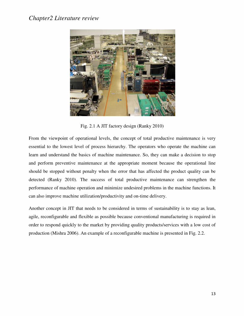
(Monden 1994). Richard et al. (2010) proposed that the implementations of JIT (see Fig. 2.1)
such as focused factory, reduced setup times, group technology, total productive maintenance,
multifunction employees, uniform workload, just-in-time purchasing, Kanban, total quality
control and quality circles should be accomplished by organizations in order to achieve
sustainable operations (Richard 2010). In addition, Ranky et al. (2010) also suggest the
application of a lean and green design concept to gain sustainable green, eco-friendly, quality
products that satisfy customer needs and produce the exact amount demanded. This can lead to a
reduction in inventory waste and cost throughout the whole supply network (Ranky 2010). From
this advantage, the concept of a pull system that integrates flexibility and real time response can,
therefore, play an important role in the ERP model (Chin-Tsai L. 2011).
Chapter2 Literature review
13
Fig. 2.1 A JIT factory design (Ranky 2010)
From the viewpoint of operational levels, the concept of total productive maintenance is very
essential to the lowest level of process hierarchy. The operators who operate the machine can
learn and understand the basics of machine maintenance. So, they can make a decision to stop
and perform preventive maintenance at the appropriate moment because the operational line
should be stopped without penalty when the error that has affected the product quality can be
detected (Ranky 2010). The success of total productive maintenance can strengthen the
performance of machine operation and minimize undesired problems in the machine functions. It
can also improve machine utilization/productivity and on-time delivery.
Another concept in JIT that needs to be considered in terms of sustainability is to stay as lean,
agile, reconfigurable and flexible as possible because conventional manufacturing is required in
order to respond quickly to the market by providing quality products/services with a low cost of
production (Mishra 2006). An example of a reconfigurable machine is presented in Fig. 2.2.
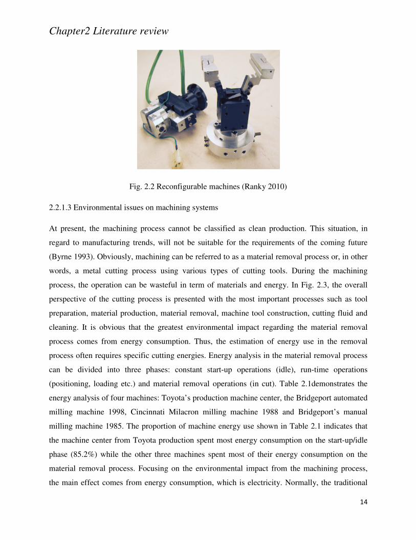
Chapter2 Literature review
14
Fig. 2.2 Reconfigurable machines (Ranky 2010)
2.2.1.3 Environmental issues on machining systems
At present, the machining process cannot be classified as clean production. This situation, in
regard to manufacturing trends, will not be suitable for the requirements of the coming future
(Byrne 1993). Obviously, machining can be referred to as a material removal process or, in other
words, a metal cutting process using various types of cutting tools. During the machining
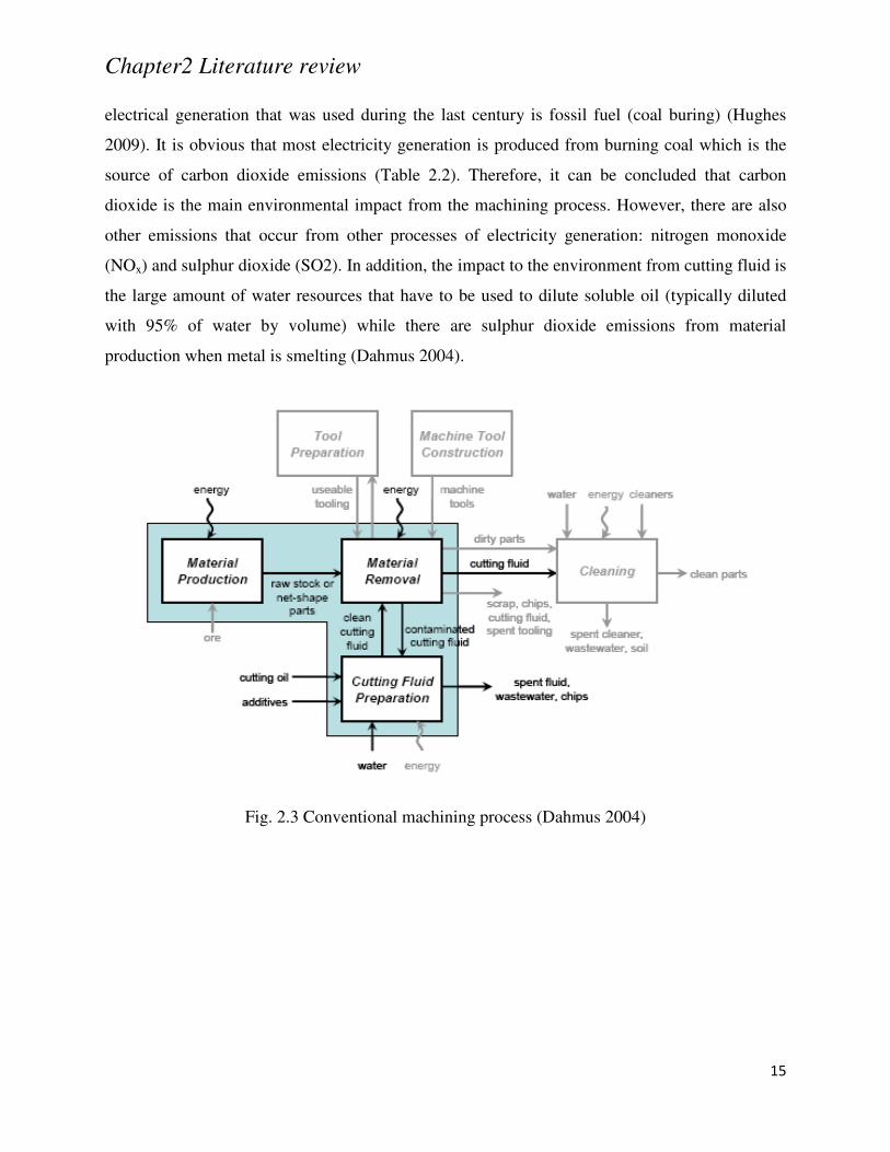
process, the operation can be wasteful in term of materials and energy. In Fig. 2.3, the overall
perspective of the cutting process is presented with the most important processes such as tool
preparation, material production, material removal, machine tool construction, cutting fluid and
cleaning. It is obvious that the greatest environmental impact regarding the material removal
process comes from energy consumption. Thus, the estimation of energy use in the removal
process often requires specific cutting energies. Energy analysis in the material removal process
can be divided into three phases: constant start-up operations (idle), run-time operations
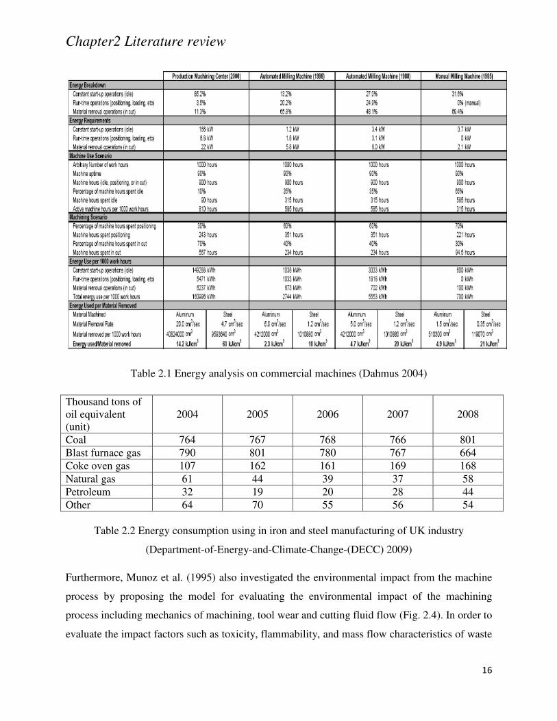
(positioning, loading etc.) and material removal operations (in cut). Table 2.1demonstrates the
energy analysis of four machines: Toyota’s production machine center, the Bridgeport automated
milling machine 1998, Cincinnati Milacron milling machine 1988 and Bridgeport’s manual
milling machine 1985. The proportion of machine energy use shown in Table 2.1 indicates that
the machine center from Toyota production spent most energy consumption on the start-up/idle
phase (85.2%) while the other three machines spent most of their energy consumption on the
material removal process. Focusing on the environmental impact from the machining process,
the main effect comes from energy consumption, which is electricity. Normally, the traditional
Chapter2 Literature review
15
electrical generation that was used during the last century is fossil fuel (coal buring) (Hughes
2009). It is obvious that most electricity generation is produced from burning coal which is the
source of carbon dioxide emissions (Table 2.2). Therefore, it can be concluded that carbon
dioxide is the main environmental impact from the machining process. However, there are also
other emissions that occur from other processes of electricity generation: nitrogen monoxide
(NOx) and sulphur dioxide (SO2). In addition, the impact to the environment from cutting fluid is
the large amount of water resources that have to be used to dilute soluble oil (typically diluted
with 95% of water by volume) while there are sulphur dioxide emissions from material
production when metal is smelting (Dahmus 2004).
Fig. 2.3 Conventional machining process (Dahmus 2004)
Chapter2 Literature review
16
Table 2.1 Energy analysis on commercial machines (Dahmus 2004)
Thousand tons of oil equivalent (unit)
2004 2005 2006 2007 2008
Coal 764 767 768 766 801 Blast furnace gas 790 801 780 767 664
Coke oven gas 107 162 161 169 168
Natural gas 61 44 39 37 58 Petroleum 32 19 20 28 44
Other 64 70 55 56 54
Table 2.2 Energy consumption using in iron and steel manufacturing of UK industry
(Department-of-Energy-and-Climate-Change-(DECC) 2009)
Furthermore, Munoz et al. (1995) also investigated the environmental impact from the machine
process by proposing the model for evaluating the environmental impact of the machining
process including mechanics of machining, tool wear and cutting fluid flow (Fig. 2.4). In order to
evaluate the impact factors such as toxicity, flammability, and mass flow characteristics of waste
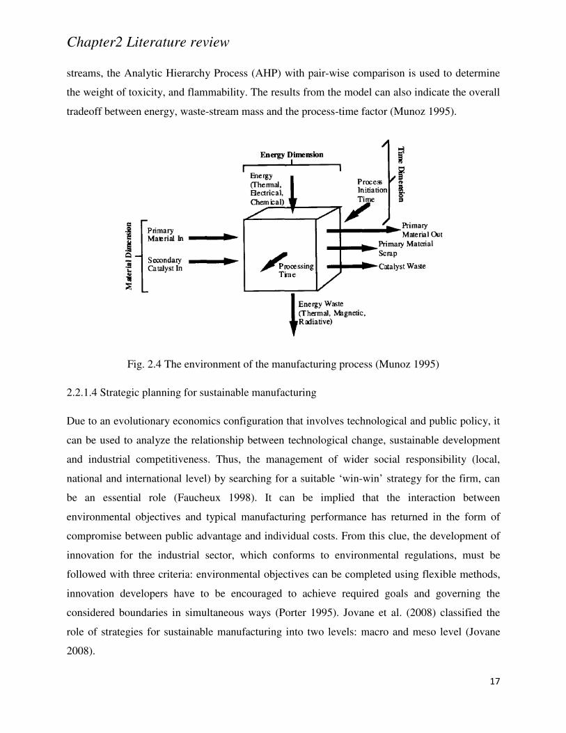
Chapter2 Literature review
17
streams, the Analytic Hierarchy Process (AHP) with pair-wise comparison is used to determine
the weight of toxicity, and flammability. The results from the model can also indicate the overall
tradeoff between energy, waste-stream mass and the process-time factor (Munoz 1995).
Fig. 2.4 The environment of the manufacturing process (Munoz 1995)
2.2.1.4 Strategic planning for sustainable manufacturing
Due to an evolutionary economics configuration that involves technological and public policy, it
can be used to analyze the relationship between technological change, sustainable development
and industrial competitiveness. Thus, the management of wider social responsibility (local,
national and international level) by searching for a suitable ‘win-win’ strategy for the firm, can
be an essential role (Faucheux 1998). It can be implied that the interaction between
environmental objectives and typical manufacturing performance has returned in the form of
compromise between public advantage and individual costs. From this clue, the development of
innovation for the industrial sector, which conforms to environmental regulations, must be
followed with three criteria: environmental objectives can be completed using flexible methods,
innovation developers have to be encouraged to achieve required goals and governing the
considered boundaries in simultaneous ways (Porter 1995). Jovane et al. (2008) classified the
role of strategies for sustainable manufacturing into two levels: macro and meso level (Jovane
2008).

Chapter2 Literature review
18
Considering the macro level of sustainable manufacturing, the implementation of environmental
concern is considered to be the essential key factor while the economic issue is used as a tool for
accessing the social dimension. In the last decade, many countries have been developing their
international and domestic policies to catch up with environmental concerns while economic and
social perspectives are still moving in the right direction. For example, the Department of
Commerce governed by the US government, aims to support the co-operation between public
and private sectors to achieve effective sustainable manufacturing as a result of the requirements
of global competitiveness (United States Department of Commerce 2004). In China, the
awareness of the importance of energy policy is now taken into account due to the rapid
expansion of the China’s economy which requires large amounts of energy consumption (70% of
China’s primary energy supply is coal). Thus, China has been taking action to enable the role of
renewable energy and R&D as a top-down approach in the form of policy. The proposal of this
policy aims to gather energy conservation and economic support together. For instance, the
Chinese government applied the regulation of an electricity surcharge by 0.2 cent/kWh in order
to support the use of renewable energy while the Ministry of Finance launched a new regulation
for the import of wind turbines by refunding tax in order to stimulate the utilization of wind
energy (Chai 2010).
At the meso level, the characteristic of sustainable manufacturing relies on products/services,
processes and business models that are related to economical, social and environmental topics.
Hence, many researchers have been trying to make efforts to develop strategies associated with
products/services life cycles and enterprise business models. For instance, Tomiya proposed a
developed conception called the Poss Mass Production Paradigm (PMPP), which aims to
disconnect the explanation of economics from a material and energy consumption angle while
the quality of life issue can be satisfied based on the conventional life cycle model (Fig. 2.5). To
implement this concept, the idea of closing the life cycle loop, which refers to recycling,
remanufacturing, refurbishing, cascading and reuse, is used as the main methodology to reduce
the production of artifacts (Tomiya 1999). For another example of developed modelling, Kuhtz
et al. (2010) proposed the application of using an enterprise input-output model (EIO) to
investigate the amount of energy consumptions together with the pollution levels of tile
manufacturing (Fig. 2.6). According to the operational mechanism of this model, the flow (raw
material, energy, product and waste etc.) of the considered manufacturing line evaluates how the
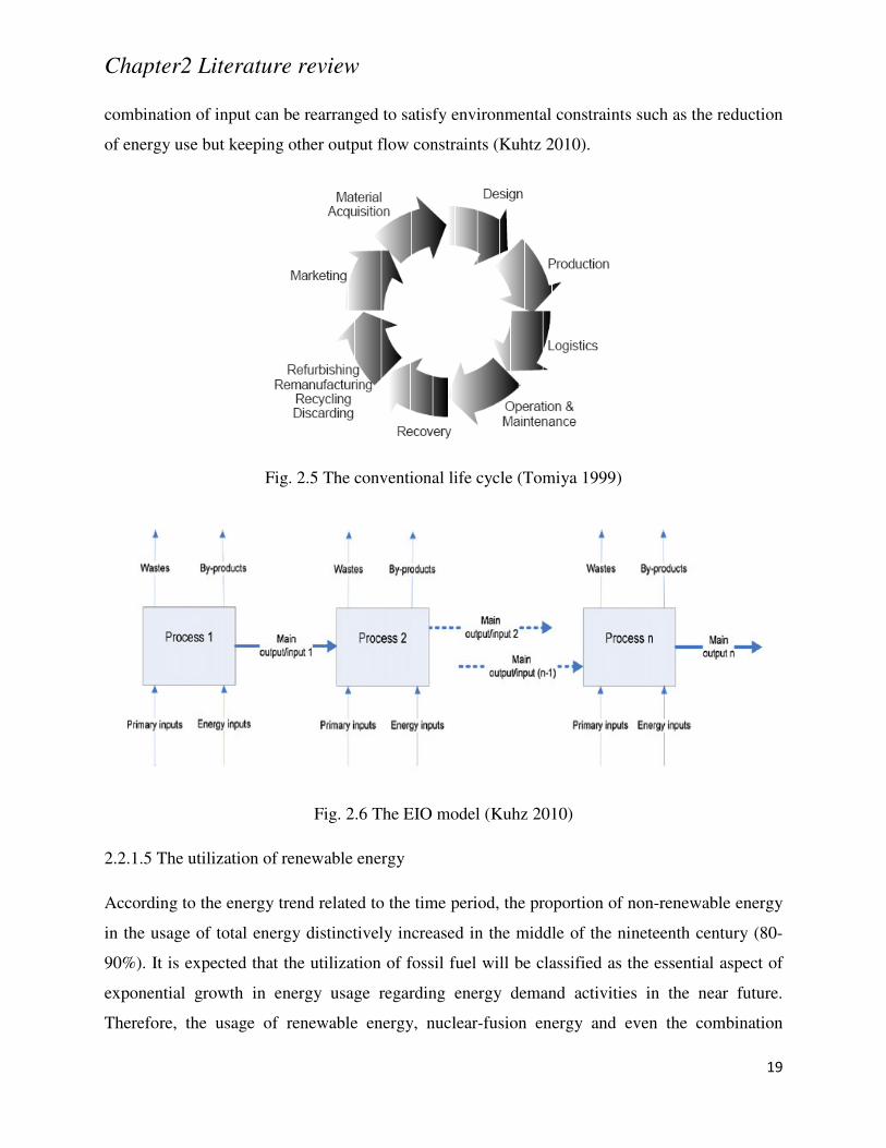
Chapter2 Literature review
19
combination of input can be rearranged to satisfy environmental constraints such as the reduction
of energy use but keeping other output flow constraints (Kuhtz 2010).
Fig. 2.5 The conventional life cycle (Tomiya 1999)
Fig. 2.6 The EIO model (Kuhz 2010)
2.2.1.5 The utilization of renewable energy
According to the energy trend related to the time period, the proportion of non-renewable energy
in the usage of total energy distinctively increased in the middle of the nineteenth century (80-
90%). It is expected that the utilization of fossil fuel will be classified as the essential aspect of
exponential growth in energy usage regarding energy demand activities in the near future.
Therefore, the usage of renewable energy, nuclear-fusion energy and even the combination
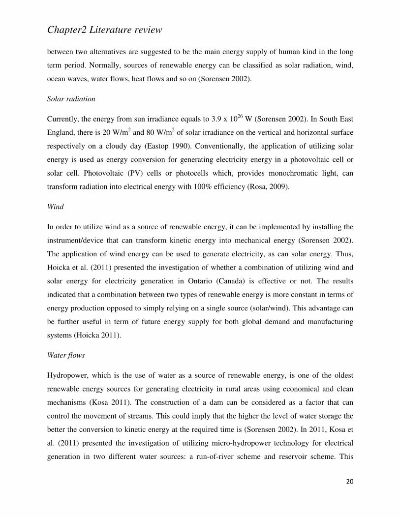
Chapter2 Literature review
20
between two alternatives are suggested to be the main energy supply of human kind in the long
term period. Normally, sources of renewable energy can be classified as solar radiation, wind,
ocean waves, water flows, heat flows and so on (Sorensen 2002).
Solar radiation
Currently, the energy from sun irradiance equals to 3.9 x 1026 W (Sorensen 2002). In South East
England, there is 20 W/m2 and 80 W/m2 of solar irradiance on the vertical and horizontal surface
respectively on a cloudy day (Eastop 1990). Conventionally, the application of utilizing solar
energy is used as energy conversion for generating electricity energy in a photovoltaic cell or
solar cell. Photovoltaic (PV) cells or photocells which, provides monochromatic light, can
transform radiation into electrical energy with 100% efficiency (Rosa, 2009).
Wind
In order to utilize wind as a source of renewable energy, it can be implemented by installing the
instrument/device that can transform kinetic energy into mechanical energy (Sorensen 2002).
The application of wind energy can be used to generate electricity, as can solar energy. Thus,
Hoicka et al. (2011) presented the investigation of whether a combination of utilizing wind and
solar energy for electricity generation in Ontario (Canada) is effective or not. The results
indicated that a combination between two types of renewable energy is more constant in terms of
energy production opposed to simply relying on a single source (solar/wind). This advantage can
be further useful in term of future energy supply for both global demand and manufacturing
systems (Hoicka 2011).
Water flows
Hydropower, which is the use of water as a source of renewable energy, is one of the oldest
renewable energy sources for generating electricity in rural areas using economical and clean
mechanisms (Kosa 2011). The construction of a dam can be considered as a factor that can
control the movement of streams. This could imply that the higher the level of water storage the
better the conversion to kinetic energy at the required time is (Sorensen 2002). In 2011, Kosa et
al. (2011) presented the investigation of utilizing micro-hydropower technology for electrical
generation in two different water sources: a run-of-river scheme and reservoir scheme. This
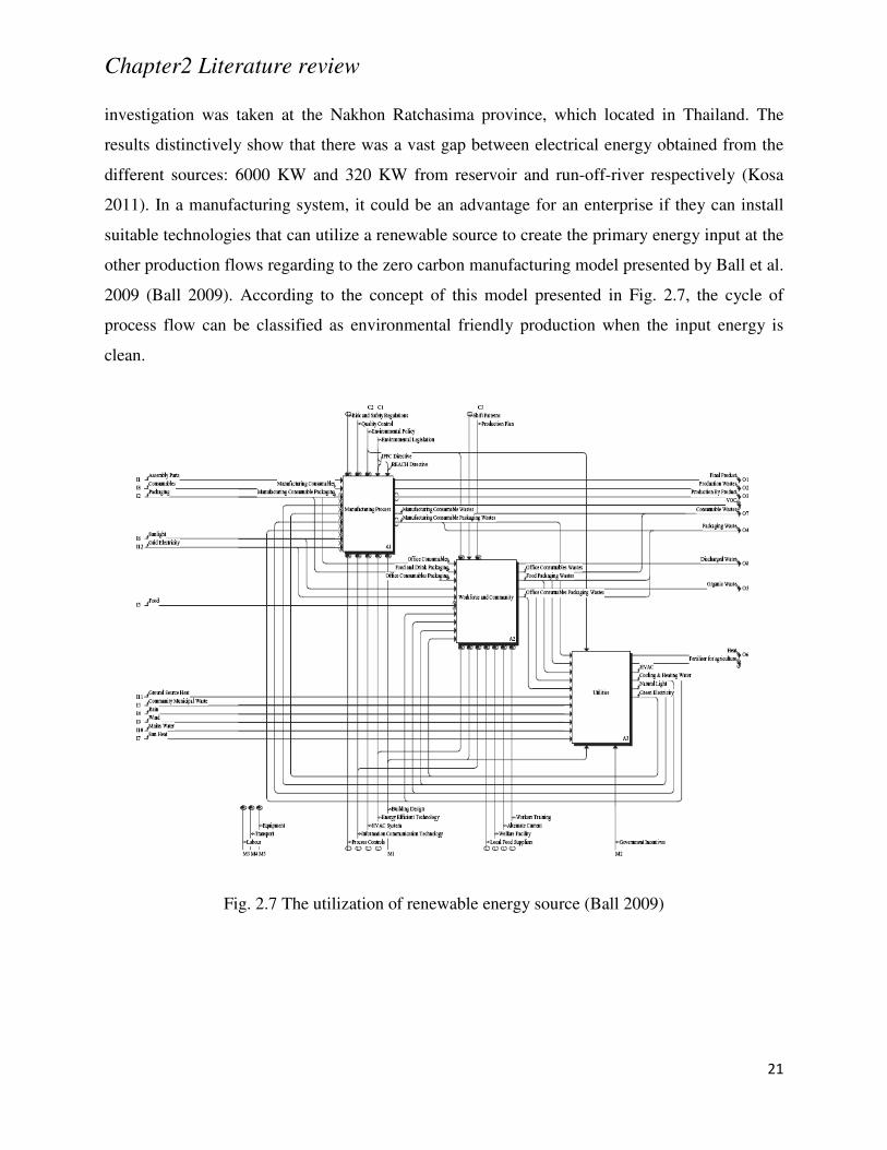
Chapter2 Literature review
21
investigation was taken at the Nakhon Ratchasima province, which located in Thailand. The
results distinctively show that there was a vast gap between electrical energy obtained from the
different sources: 6000 KW and 320 KW from reservoir and run-off-river respectively (Kosa
2011). In a manufacturing system, it could be an advantage for an enterprise if they can install
suitable technologies that can utilize a renewable source to create the primary energy input at the
other production flows regarding to the zero carbon manufacturing model presented by Ball et al.
2009 (Ball 2009). According to the concept of this model presented in Fig. 2.7, the cycle of
process flow can be classified as environmental friendly production when the input energy is
clean.
Fig. 2.7 The utilization of renewable energy source (Ball 2009)
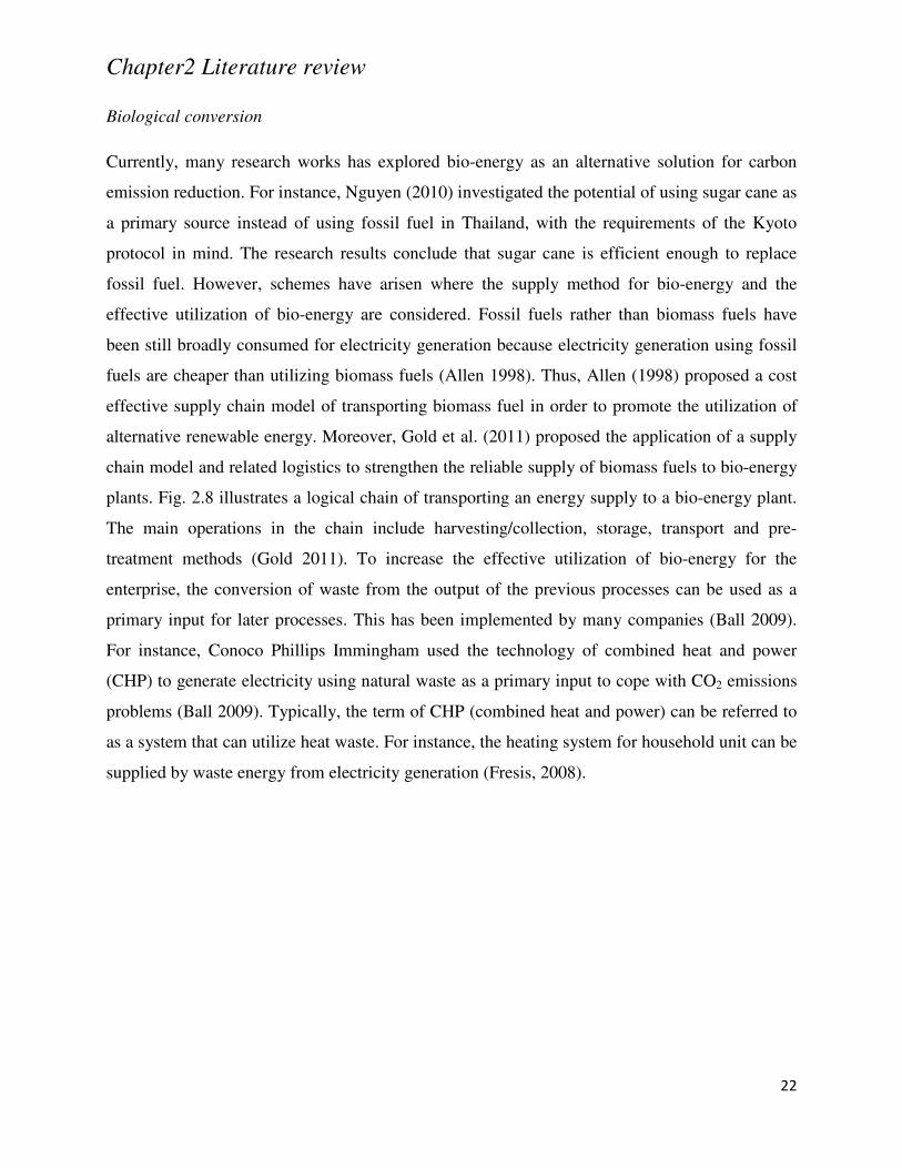
Chapter2 Literature review
22
Biological conversion
Currently, many research works has explored bio-energy as an alternative solution for carbon
emission reduction. For instance, Nguyen (2010) investigated the potential of using sugar cane as
a primary source instead of using fossil fuel in Thailand, with the requirements of the Kyoto
protocol in mind. The research results conclude that sugar cane is efficient enough to replace
fossil fuel. However, schemes have arisen where the supply method for bio-energy and the
effective utilization of bio-energy are considered. Fossil fuels rather than biomass fuels have
been still broadly consumed for electricity generation because electricity generation using fossil
fuels are cheaper than utilizing biomass fuels (Allen 1998). Thus, Allen (1998) proposed a cost
effective supply chain model of transporting biomass fuel in order to promote the utilization of
alternative renewable energy. Moreover, Gold et al. (2011) proposed the application of a supply
chain model and related logistics to strengthen the reliable supply of biomass fuels to bio-energy
plants. Fig. 2.8 illustrates a logical chain of transporting an energy supply to a bio-energy plant.
The main operations in the chain include harvesting/collection, storage, transport and pre-
treatment methods (Gold 2011). To increase the effective utilization of bio-energy for the
enterprise, the conversion of waste from the output of the previous processes can be used as a
primary input for later processes. This has been implemented by many companies (Ball 2009).
For instance, Conoco Phillips Immingham used the technology of combined heat and power
(CHP) to generate electricity using natural waste as a primary input to cope with CO2 emissions
problems (Ball 2009). Typically, the term of CHP (combined heat and power) can be referred to
as a system that can utilize heat waste. For instance, the heating system for household unit can be
supplied by waste energy from electricity generation (Fresis, 2008).
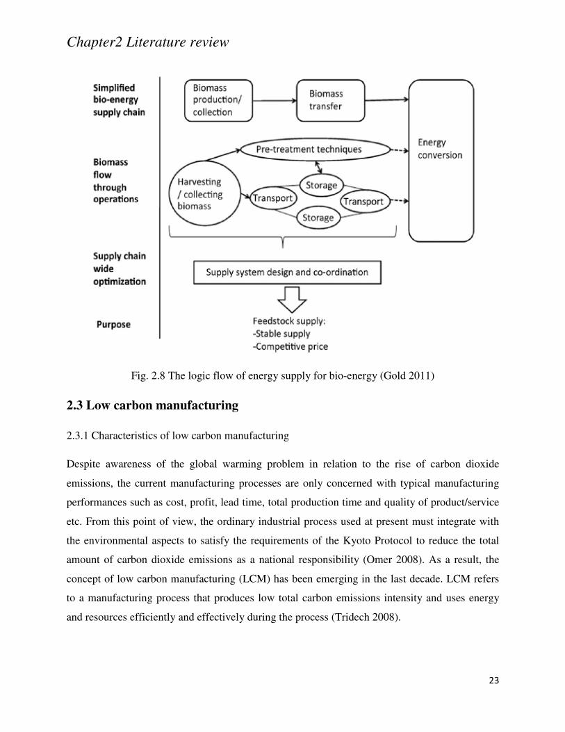
Chapter2 Literature review
23
Fig. 2.8 The logic flow of energy supply for bio-energy (Gold 2011)
2.3 Low carbon manufacturing
2.3.1 Characteristics of low carbon manufacturing
Despite awareness of the global warming problem in relation to the rise of carbon dioxide
emissions, the current manufacturing processes are only concerned with typical manufacturing
performances such as cost, profit, lead time, total production time and quality of product/service
etc. From this point of view, the ordinary industrial process used at present must integrate with
the environmental aspects to satisfy the requirements of the Kyoto Protocol to reduce the total
amount of carbon dioxide emissions as a national responsibility (Omer 2008). As a result, the
concept of low carbon manufacturing (LCM) has been emerging in the last decade. LCM refers
to a manufacturing process that produces low total carbon emissions intensity and uses energy
and resources efficiently and effectively during the process (Tridech 2008).
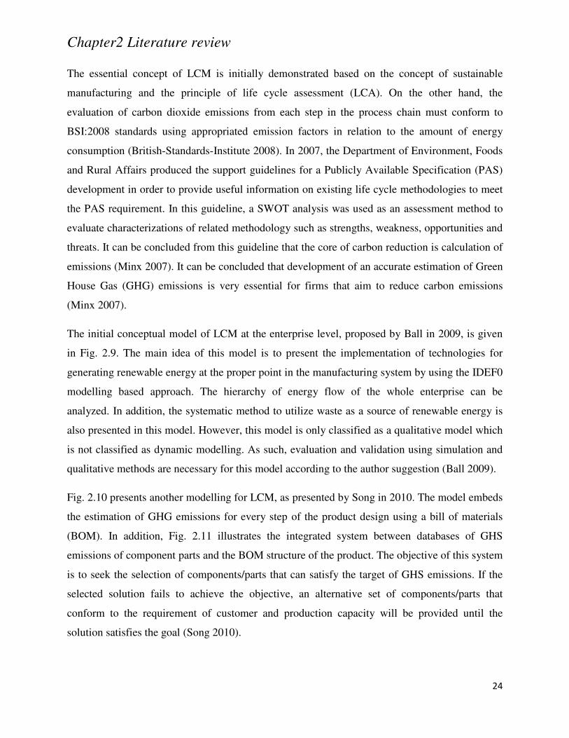
Chapter2 Literature review
24
The essential concept of LCM is initially demonstrated based on the concept of sustainable
manufacturing and the principle of life cycle assessment (LCA). On the other hand, the
evaluation of carbon dioxide emissions from each step in the process chain must conform to
BSI:2008 standards using appropriated emission factors in relation to the amount of energy
consumption (British-Standards-Institute 2008). In 2007, the Department of Environment, Foods
and Rural Affairs produced the support guidelines for a Publicly Available Specification (PAS)
development in order to provide useful information on existing life cycle methodologies to meet
the PAS requirement. In this guideline, a SWOT analysis was used as an assessment method to
evaluate characterizations of related methodology such as strengths, weakness, opportunities and
threats. It can be concluded from this guideline that the core of carbon reduction is calculation of
emissions (Minx 2007). It can be concluded that development of an accurate estimation of Green
House Gas (GHG) emissions is very essential for firms that aim to reduce carbon emissions
(Minx 2007).
The initial conceptual model of LCM at the enterprise level, proposed by Ball in 2009, is given
in Fig. 2.9. The main idea of this model is to present the implementation of technologies for
generating renewable energy at the proper point in the manufacturing system by using the IDEF0
modelling based approach. The hierarchy of energy flow of the whole enterprise can be
analyzed. In addition, the systematic method to utilize waste as a source of renewable energy is
also presented in this model. However, this model is only classified as a qualitative model which
is not classified as dynamic modelling. As such, evaluation and validation using simulation and
qualitative methods are necessary for this model according to the author suggestion (Ball 2009).
Fig. 2.10 presents another modelling for LCM, as presented by Song in 2010. The model embeds
the estimation of GHG emissions for every step of the product design using a bill of materials
(BOM). In addition, Fig. 2.11 illustrates the integrated system between databases of GHS
emissions of component parts and the BOM structure of the product. The objective of this system
is to seek the selection of components/parts that can satisfy the target of GHS emissions. If the
selected solution fails to achieve the objective, an alternative set of components/parts that
conform to the requirement of customer and production capacity will be provided until the
solution satisfies the goal (Song 2010).
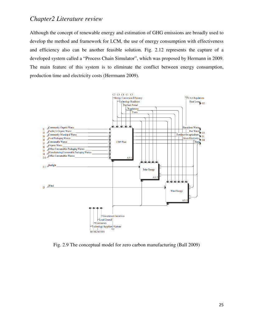
Chapter2 Literature review
25
Although the concept of renewable energy and estimation of GHG emissions are broadly used to
develop the method and framework for LCM, the use of energy consumption with effectiveness
and efficiency also can be another feasible solution. Fig. 2.12 represents the capture of a
developed system called a “Process Chain Simulator”, which was proposed by Hermann in 2009.
The main feature of this system is to eliminate the conflict between energy consumption,
production time and electricity costs (Herrmann 2009).
Fig. 2.9 The conceptual model for zero carbon manufacturing (Ball 2009)
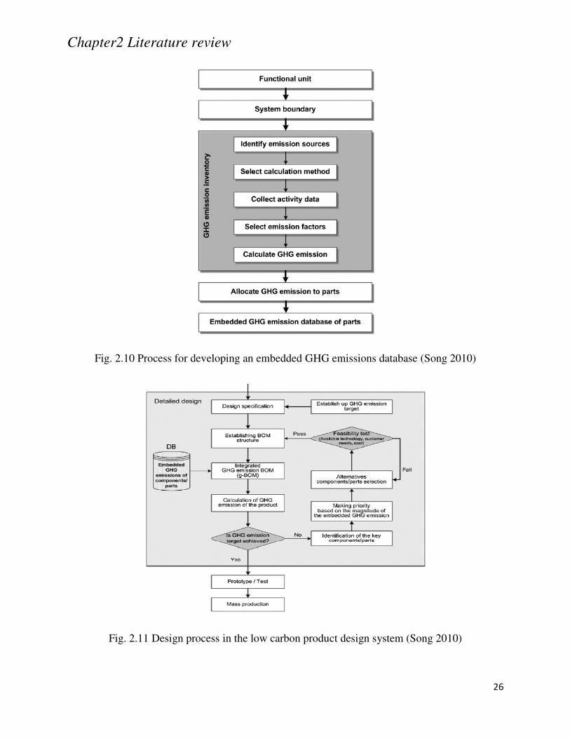
Chapter2 Literature review
26
Fig. 2.10 Process for developing an embedded GHG emissions database (Song 2010)
Fig. 2.11 Design process in the low carbon product design system (Song 2010)
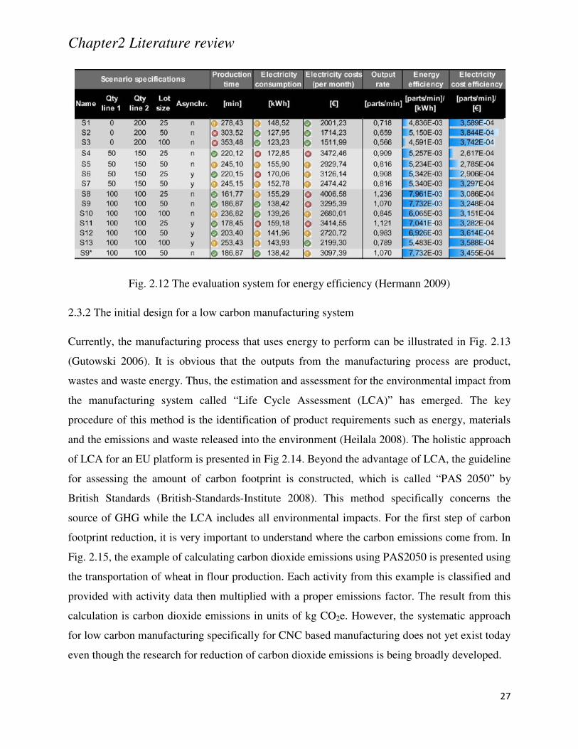
Chapter2 Literature review
27
Fig. 2.12 The evaluation system for energy efficiency (Hermann 2009)
2.3.2 The initial design for a low carbon manufacturing system
Currently, the manufacturing process that uses energy to perform can be illustrated in Fig. 2.13
(Gutowski 2006). It is obvious that the outputs from the manufacturing process are product,
wastes and waste energy. Thus, the estimation and assessment for the environmental impact from
the manufacturing system called “Life Cycle Assessment (LCA)” has emerged. The key
procedure of this method is the identification of product requirements such as energy, materials
and the emissions and waste released into the environment (Heilala 2008). The holistic approach
of LCA for an EU platform is presented in Fig 2.14. Beyond the advantage of LCA, the guideline
for assessing the amount of carbon footprint is constructed, which is called “PAS 2050” by
British Standards (British-Standards-Institute 2008). This method specifically concerns the
source of GHG while the LCA includes all environmental impacts. For the first step of carbon
footprint reduction, it is very important to understand where the carbon emissions come from. In
Fig. 2.15, the example of calculating carbon dioxide emissions using PAS2050 is presented using
the transportation of wheat in flour production. Each activity from this example is classified and
provided with activity data then multiplied with a proper emissions factor. The result from this
calculation is carbon dioxide emissions in units of kg CO2e. However, the systematic approach
for low carbon manufacturing specifically for CNC based manufacturing does not yet exist today
even though the research for reduction of carbon dioxide emissions is being broadly developed.
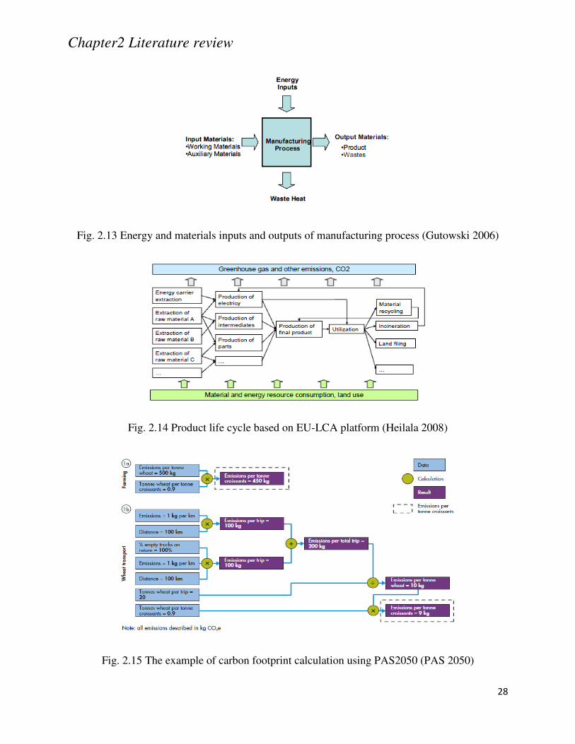
Chapter2 Literature review
28
Fig. 2.13 Energy and materials inputs and outputs of manufacturing process (Gutowski 2006)
Fig. 2.14 Product life cycle based on EU-LCA platform (Heilala 2008)
Fig. 2.15 The example of carbon footprint calculation using PAS2050 (PAS 2050)
Chapter2 Literature review
29
2.4 Multi-criteria decision making techniques
Typically, the term multi-criteria decision making (MCDM) can refers to the method used to
solve the conflict between objectives and return the proper solution from the set of alternative
solutions. Normally, the configuration of MCDM, which is a branch of Operations Research
(OR) models can be categorized into Multi-Objective Decision Making (MODM) and Multi-
Attribute Decision Making (MADM) (Pohekar 2004; Pohekar 2004; Cristobal 2011).
The main distinction between MODM and MADM is their method of the decision making
process. For the MODM, the problem details are transformed into a mathematical formulation
which has three main parts: objective functions, constraints and range of decision variables.
After the mathematical formulation was completed, all equations are arranged into matrix
vectors that are ready for the optimization algorithm. The result of using the MODM method is
the best alternative (optimal solution) which can satisfy all objectives functions in the considered
problem formulation. On the other hand, it can be implied that alternative solutions from the
MODM method are not predetermined regarding, the only optimal solution that can return from
the optimization process. In the scope of Operations Research, types of mathematical
formulation are linear programming, multi-objective/goal programming, integer programming,
fuzzy programming and nonlinear programming. For MADM, each possible alternative is
predetermined before the best solution is returned to the decision maker. Typically, the structure
of MADM consists of goal, criteria and possible alternatives. The normalization of value and
comparison methods are used in the decision process when MADM is selected to find out the
best solution. MODM and MADM are compatible with quantitative and qualitative problems
(Cristobal 2011). The example of contemporary MADM methods used in decision making in
various fields are an Analytical Hierarchy Process (AHP), PROMETHEE, ELECTRE and Multi-
attribute utility theory etc. In the next section, the details of related decision making methods
used in this research are discussed.
2.4.1 Analytical Hierarchy Process (AHP)
According to the fundamentals of the AHP method, it was firstly demonstrated by Saaty in 1980
(Saaty 2008). The procedure for seeking the best solution in AHP is a top-down process by
decomposing the goal into criteria/sub criteria and alternative solutions at the bottom level. All
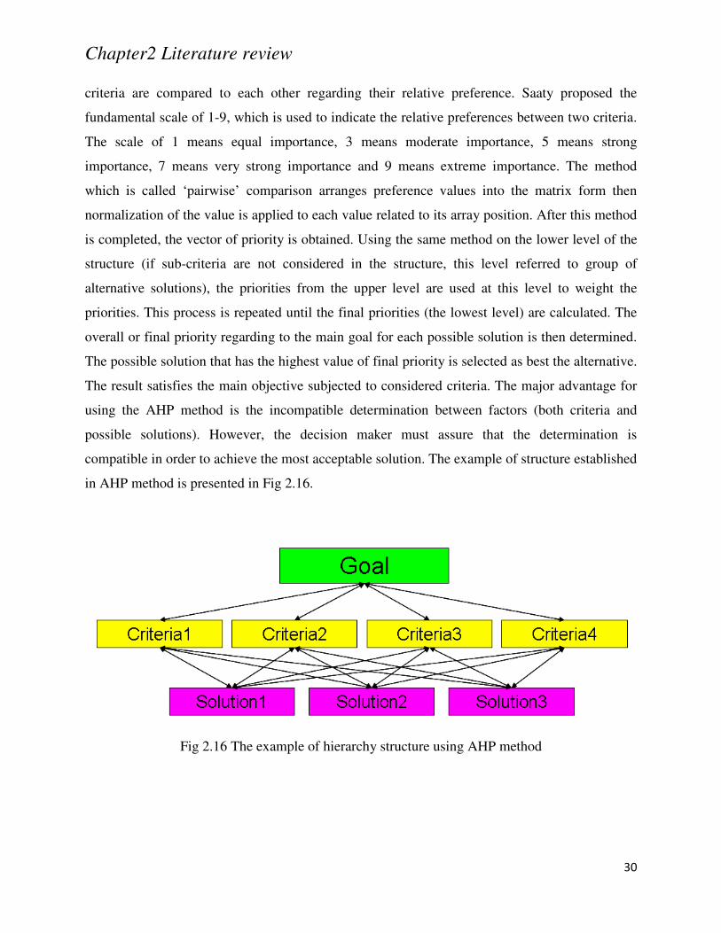
Chapter2 Literature review
30
criteria are compared to each other regarding their relative preference. Saaty proposed the
fundamental scale of 1-9, which is used to indicate the relative preferences between two criteria.
The scale of 1 means equal importance, 3 means moderate importance, 5 means strong
importance, 7 means very strong importance and 9 means extreme importance. The method
which is called ‘pairwise’ comparison arranges preference values into the matrix form then
normalization of the value is applied to each value related to its array position. After this method
is completed, the vector of priority is obtained. Using the same method on the lower level of the
structure (if sub-criteria are not considered in the structure, this level referred to group of
alternative solutions), the priorities from the upper level are used at this level to weight the
priorities. This process is repeated until the final priorities (the lowest level) are calculated. The
overall or final priority regarding to the main goal for each possible solution is then determined.
The possible solution that has the highest value of final priority is selected as best the alternative.
The result satisfies the main objective subjected to considered criteria. The major advantage for
using the AHP method is the incompatible determination between factors (both criteria and
possible solutions). However, the decision maker must assure that the determination is
compatible in order to achieve the most acceptable solution. The example of structure established
in AHP method is presented in Fig 2.16.
Fig 2.16 The example of hierarchy structure using AHP method
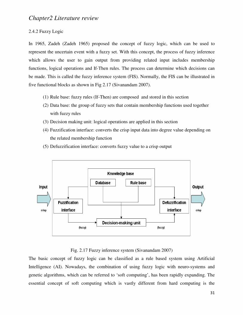
Chapter2 Literature review
31
2.4.2 Fuzzy Logic
In 1965, Zadeh (Zadeh 1965) proposed the concept of fuzzy logic, which can be used to
represent the uncertain event with a fuzzy set. With this concept, the process of fuzzy inference
which allows the user to gain output from providing related input includes membership
functions, logical operations and If-Then rules. The process can determine which decisions can
be made. This is called the fuzzy inference system (FIS). Normally, the FIS can be illustrated in
five functional blocks as shown in Fig 2.17 (Sivanandam 2007).
(1) Rule base: fuzzy rules (If-Then) are composed and stored in this section
(2) Data base: the group of fuzzy sets that contain membership functions used together
with fuzzy rules
(3) Decision making unit: logical operations are applied in this section
(4) Fuzzification interface: converts the crisp input data into degree value depending on
the related membership function
(5) Defuzzification interface: converts fuzzy value to a crisp output
Fig. 2.17 Fuzzy inference system (Sivanandam 2007)
The basic concept of fuzzy logic can be classified as a rule based system using Artificial
Intelligence (AI). Nowadays, the combination of using fuzzy logic with neuro-systems and
genetic algorithms, which can be referred to ‘soft computing’, has been rapidly expanding. The
essential concept of soft computing which is vastly different from hard computing is the
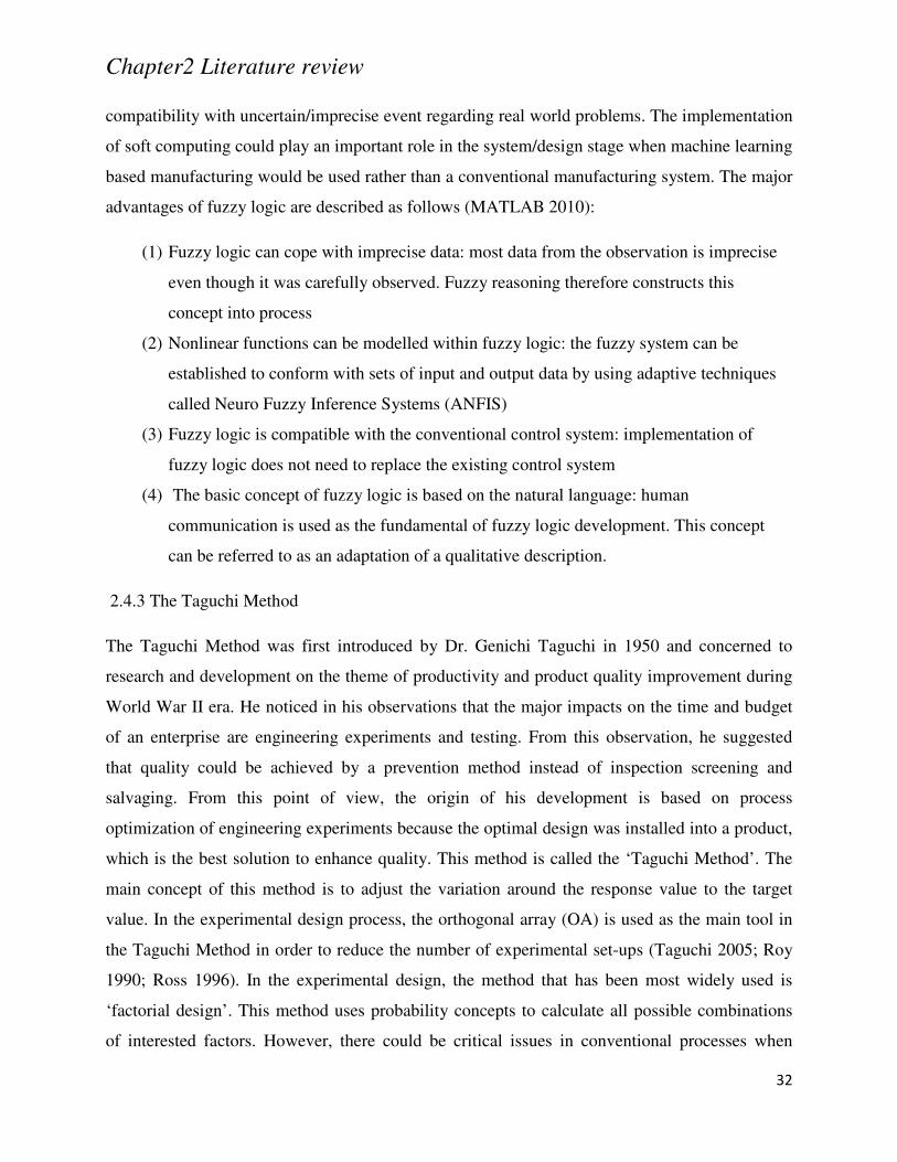
Chapter2 Literature review
32
compatibility with uncertain/imprecise event regarding real world problems. The implementation
of soft computing could play an important role in the system/design stage when machine learning
based manufacturing would be used rather than a conventional manufacturing system. The major
advantages of fuzzy logic are described as follows (MATLAB 2010):
(1) Fuzzy logic can cope with imprecise data: most data from the observation is imprecise
even though it was carefully observed. Fuzzy reasoning therefore constructs this
concept into process
(2) Nonlinear functions can be modelled within fuzzy logic: the fuzzy system can be
established to conform with sets of input and output data by using adaptive techniques
called Neuro Fuzzy Inference Systems (ANFIS)
(3) Fuzzy logic is compatible with the conventional control system: implementation of
fuzzy logic does not need to replace the existing control system
(4) The basic concept of fuzzy logic is based on the natural language: human
communication is used as the fundamental of fuzzy logic development. This concept
can be referred to as an adaptation of a qualitative description.
2.4.3 The Taguchi Method
The Taguchi Method was first introduced by Dr. Genichi Taguchi in 1950 and concerned to
research and development on the theme of productivity and product quality improvement during
World War II era. He noticed in his observations that the major impacts on the time and budget
of an enterprise are engineering experiments and testing. From this observation, he suggested
that quality could be achieved by a prevention method instead of inspection screening and
salvaging. From this point of view, the origin of his development is based on process
optimization of engineering experiments because the optimal design was installed into a product,
which is the best solution to enhance quality. This method is called the ‘Taguchi Method’. The
main concept of this method is to adjust the variation around the response value to the target
value. In the experimental design process, the orthogonal array (OA) is used as the main tool in
the Taguchi Method in order to reduce the number of experimental set-ups (Taguchi 2005; Roy
1990; Ross 1996). In the experimental design, the method that has been most widely used is
‘factorial design’. This method uses probability concepts to calculate all possible combinations
of interested factors. However, there could be critical issues in conventional processes when
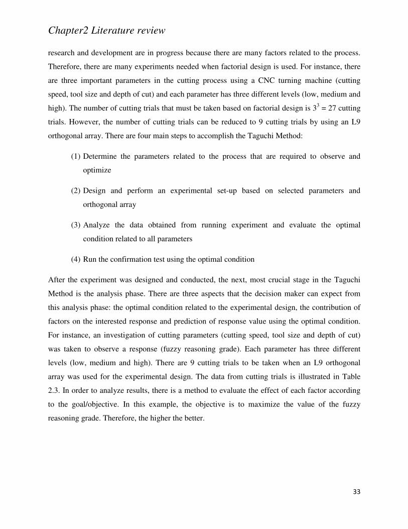
Chapter2 Literature review
33
research and development are in progress because there are many factors related to the process.
Therefore, there are many experiments needed when factorial design is used. For instance, there
are three important parameters in the cutting process using a CNC turning machine (cutting
speed, tool size and depth of cut) and each parameter has three different levels (low, medium and
high). The number of cutting trials that must be taken based on factorial design is 33 = 27 cutting
trials. However, the number of cutting trials can be reduced to 9 cutting trials by using an L9
orthogonal array. There are four main steps to accomplish the Taguchi Method:
(1) Determine the parameters related to the process that are required to observe and
optimize
(2) Design and perform an experimental set-up based on selected parameters and
orthogonal array
(3) Analyze the data obtained from running experiment and evaluate the optimal
condition related to all parameters
(4) Run the confirmation test using the optimal condition
After the experiment was designed and conducted, the next, most crucial stage in the Taguchi
Method is the analysis phase. There are three aspects that the decision maker can expect from
this analysis phase: the optimal condition related to the experimental design, the contribution of
factors on the interested response and prediction of response value using the optimal condition.
For instance, an investigation of cutting parameters (cutting speed, tool size and depth of cut)
was taken to observe a response (fuzzy reasoning grade). Each parameter has three different
levels (low, medium and high). There are 9 cutting trials to be taken when an L9 orthogonal
array was used for the experimental design. The data from cutting trials is illustrated in Table
2.3. In order to analyze results, there is a method to evaluate the effect of each factor according
to the goal/objective. In this example, the objective is to maximize the value of the fuzzy
reasoning grade. Therefore, the higher the better.
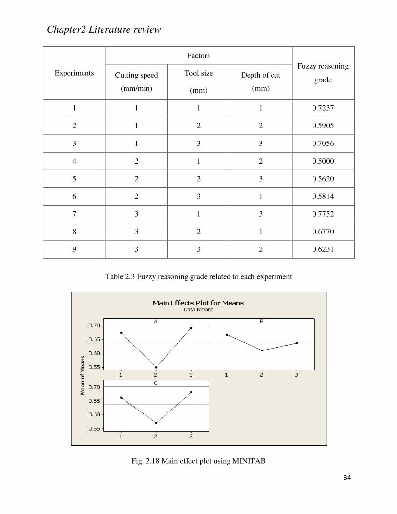
Chapter2 Literature review
34
Experiments
Factors
Fuzzy reasoning
grade Cutting speed
(mm/min)
Tool size
(mm)
Depth of cut
(mm)
1 1 1 1 0.7237
2 1 2 2 0.5905
3 1 3 3 0.7056
4 2 1 2 0.5000
5 2 2 3 0.5620
6 2 3 1 0.5814
7 3 1 3 0.7752
8 3 2 1 0.6770
9 3 3 2 0.6231
Table 2.3 Fuzzy reasoning grade related to each experiment
Fig. 2.18 Main effect plot using MINITAB
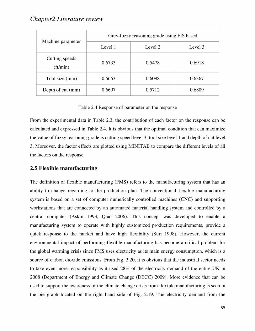
Chapter2 Literature review
35
Machine parameter Grey-fuzzy reasoning grade using FIS based
Level 1 Level 2 Level 3
Cutting speeds
(ft/min) 0.6733 0.5478 0.6918
Tool size (mm) 0.6663 0.6098 0.6367
Depth of cut (mm) 0.6607 0.5712 0.6809
Table 2.4 Response of parameter on the response
From the experimental data in Table 2.3, the contribution of each factor on the response can be
calculated and expressed in Table 2.4. It is obvious that the optimal condition that can maximize
the value of fuzzy reasoning grade is cutting speed level 3, tool size level 1 and depth of cut level
3. Moreover, the factor effects are plotted using MINITAB to compare the different levels of all
the factors on the response.
2.5 Flexible manufacturing
The definition of flexible manufacturing (FMS) refers to the manufacturing system that has an
ability to change regarding to the production plan. The conventional flexible manufacturing
system is based on a set of computer numerically controlled machines (CNC) and supporting
workstations that are connected by an automated material handling system and controlled by a
central computer (Askin 1993, Qiao 2006). This concept was developed to enable a
manufacturing system to operate with highly customized production requirements, provide a
quick response to the market and have high flexibility (Suri 1998). However, the current
environmental impact of performing flexible manufacturing has become a critical problem for
the global warming crisis since FMS uses electricity as its main energy consumption, which is a
source of carbon dioxide emissions. From Fig. 2.20, it is obvious that the industrial sector needs
to take even more responsibility as it used 28% of the electricity demand of the entire UK in
2008 (Department of Energy and Climate Change (DECC) 2009). More evidence that can be
used to support the awareness of the climate change crisis from flexible manufacturing is seen in
the pie graph located on the right hand side of Fig. 2.19. The electricity demand from the
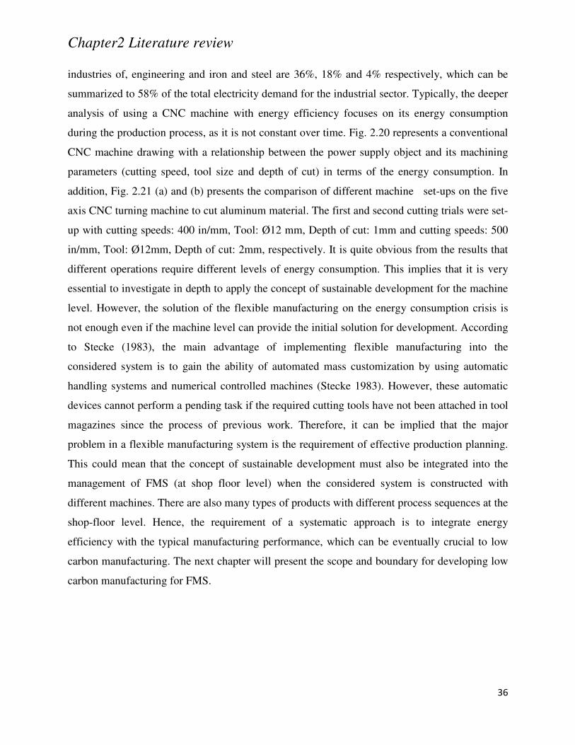
Chapter2 Literature review
36
industries of, engineering and iron and steel are 36%, 18% and 4% respectively, which can be
summarized to 58% of the total electricity demand for the industrial sector. Typically, the deeper
analysis of using a CNC machine with energy efficiency focuses on its energy consumption
during the production process, as it is not constant over time. Fig. 2.20 represents a conventional
CNC machine drawing with a relationship between the power supply object and its machining
parameters (cutting speed, tool size and depth of cut) in terms of the energy consumption. In
addition, Fig. 2.21 (a) and (b) presents the comparison of different machine set-ups on the five
axis CNC turning machine to cut aluminum material. The first and second cutting trials were set-
up with cutting speeds: 400 in/mm, Tool: Ø12 mm, Depth of cut: 1mm and cutting speeds: 500
in/mm, Tool: Ø12mm, Depth of cut: 2mm, respectively. It is quite obvious from the results that
different operations require different levels of energy consumption. This implies that it is very
essential to investigate in depth to apply the concept of sustainable development for the machine
level. However, the solution of the flexible manufacturing on the energy consumption crisis is
not enough even if the machine level can provide the initial solution for development. According
to Stecke (1983), the main advantage of implementing flexible manufacturing into the
considered system is to gain the ability of automated mass customization by using automatic
handling systems and numerical controlled machines (Stecke 1983). However, these automatic
devices cannot perform a pending task if the required cutting tools have not been attached in tool
magazines since the process of previous work. Therefore, it can be implied that the major
problem in a flexible manufacturing system is the requirement of effective production planning.
This could mean that the concept of sustainable development must also be integrated into the
management of FMS (at shop floor level) when the considered system is constructed with
different machines. There are also many types of products with different process sequences at the
shop-floor level. Hence, the requirement of a systematic approach is to integrate energy
efficiency with the typical manufacturing performance, which can be eventually crucial to low
carbon manufacturing. The next chapter will present the scope and boundary for developing low
carbon manufacturing for FMS.
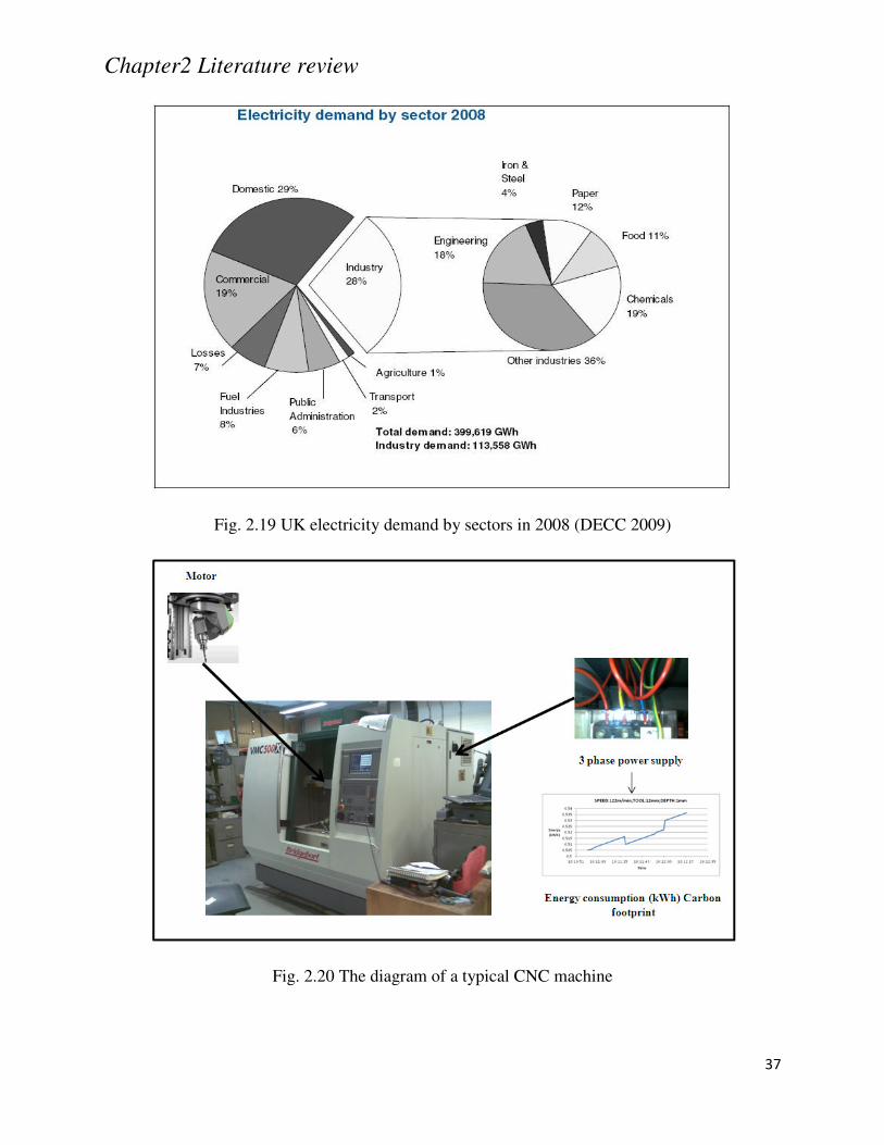
Chapter2 Literature review
37
Fig. 2.19 UK electricity demand by sectors in 2008 (DECC 2009)
Fig. 2.20 The diagram of a typical CNC machine
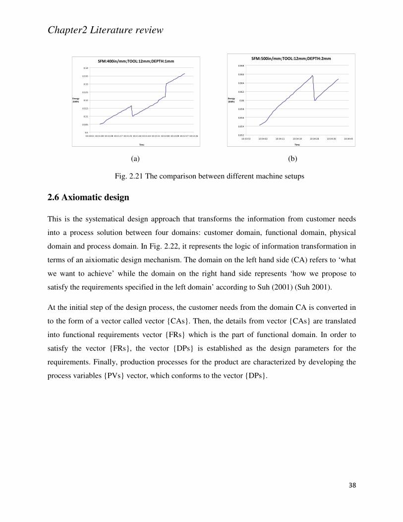
Chapter2 Literature review
38
(a) (b)
Fig. 2.21 The comparison between different machine setups
2.6 Axiomatic design
This is the systematical design approach that transforms the information from customer needs
into a process solution between four domains: customer domain, functional domain, physical
domain and process domain. In Fig. 2.22, it represents the logic of information transformation in
terms of an aixiomatic design mechanism. The domain on the left hand side (CA) refers to ‘what
we want to achieve’ while the domain on the right hand side represents ‘how we propose to
satisfy the requirements specified in the left domain’ according to Suh (2001) (Suh 2001).
At the initial step of the design process, the customer needs from the domain CA is converted in
to the form of a vector called vector CAs. Then, the details from vector CAs are translated
into functional requirements vector FRs which is the part of functional domain. In order to
satisfy the vector FRs, the vector DPs is established as the design parameters for the
requirements. Finally, production processes for the product are characterized by developing the
process variables PVs vector, which conforms to the vector DPs.
SFM:400in/mm;TOOL:12mm;DEPTH:1mm
0.5
0.505
0.51
0.515
0.52
0.525
0.53
0.535
0.54
10:10:51 10:11:00 10:11:08 10:11:17 10:11:25 10:11:34 10:11:43 10:11:51 10:12:00 10:12:09 10:12:17 10:12:26
Time
Energy
(kWh)
SFM:500in/mm;TOOL:12mm;DEPTH:2mm
0.852
0.854
0.856
0.858
0.86
0.862
0.864
0.866
0.868
10:33:53 10:34:02 10:34:11 10:34:19 10:34:28 10:34:36 10:34:45
Time
Energy
(kWh)
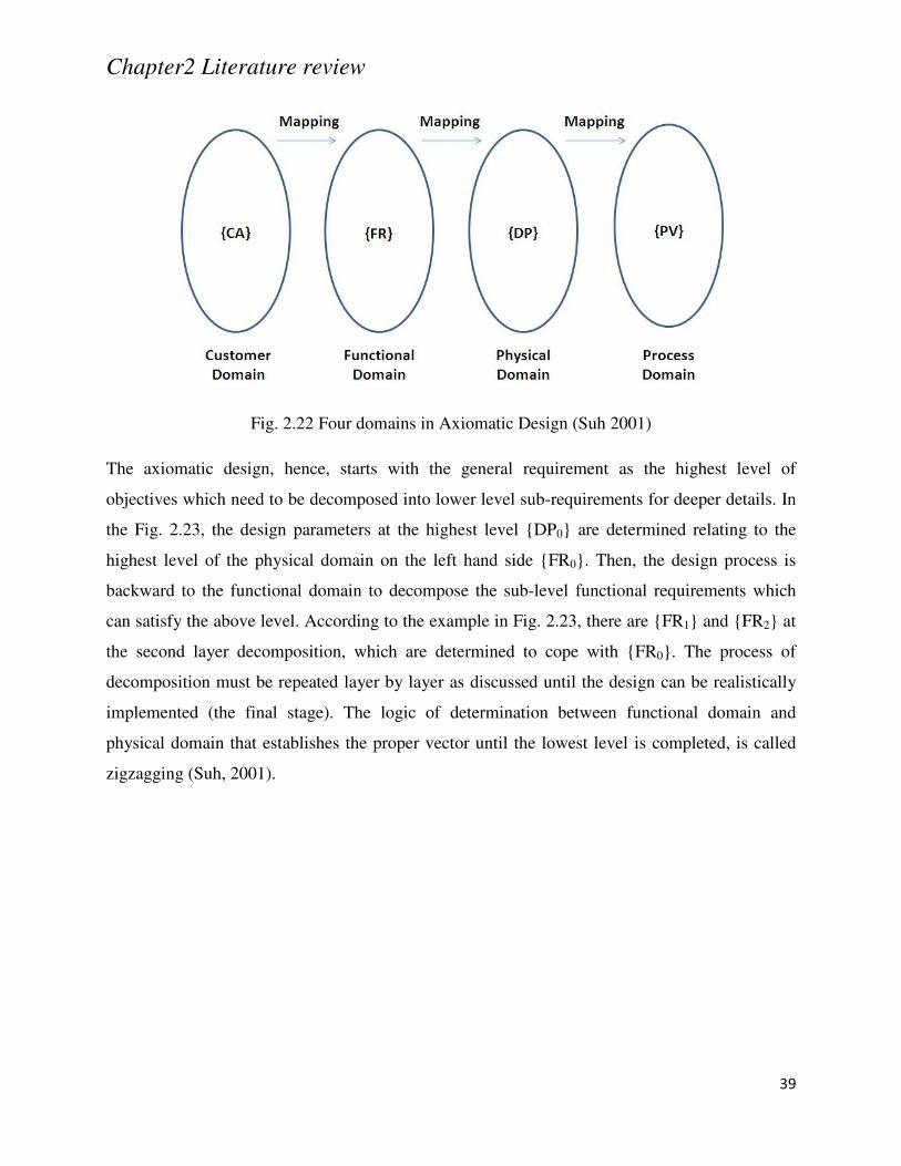
Chapter2 Literature review
39
Fig. 2.22 Four domains in Axiomatic Design (Suh 2001)
The axiomatic design, hence, starts with the general requirement as the highest level of
objectives which need to be decomposed into lower level sub-requirements for deeper details. In
the Fig. 2.23, the design parameters at the highest level DP0 are determined relating to the
highest level of the physical domain on the left hand side FR0. Then, the design process is
backward to the functional domain to decompose the sub-level functional requirements which
can satisfy the above level. According to the example in Fig. 2.23, there are FR1 and FR2 at
the second layer decomposition, which are determined to cope with FR0. The process of
decomposition must be repeated layer by layer as discussed until the design can be realistically
implemented (the final stage). The logic of determination between functional domain and
physical domain that establishes the proper vector until the lowest level is completed, is called
zigzagging (Suh, 2001).
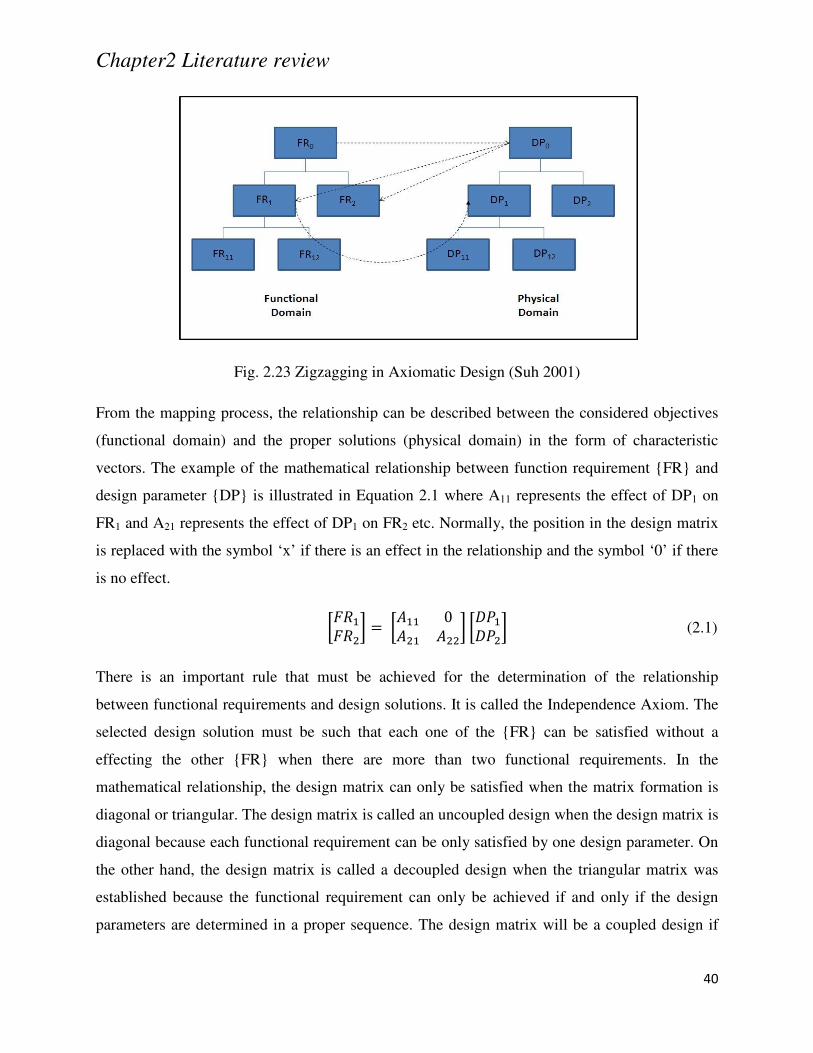
Chapter2 Literature review
40
Fig. 2.23 Zigzagging in Axiomatic Design (Suh 2001)
From the mapping process, the relationship can be described between the considered objectives
(functional domain) and the proper solutions (physical domain) in the form of characteristic
vectors. The example of the mathematical relationship between function requirement FR and
design parameter DP is illustrated in Equation 2.1 where A11 represents the effect of DP1 on
FR1 and A21 represents the effect of DP1 on FR2 etc. Normally, the position in the design matrix
is replaced with the symbol ‘x’ if there is an effect in the relationship and the symbol ‘0’ if there
is no effect.
0 (2.1)
There is an important rule that must be achieved for the determination of the relationship
between functional requirements and design solutions. It is called the Independence Axiom. The
selected design solution must be such that each one of the FR can be satisfied without a
effecting the other FR when there are more than two functional requirements. In the
mathematical relationship, the design matrix can only be satisfied when the matrix formation is
diagonal or triangular. The design matrix is called an uncoupled design when the design matrix is
diagonal because each functional requirement can be only satisfied by one design parameter. On
the other hand, the design matrix is called a decoupled design when the triangular matrix was
established because the functional requirement can only be achieved if and only if the design
parameters are determined in a proper sequence. The design matrix will be a coupled design if
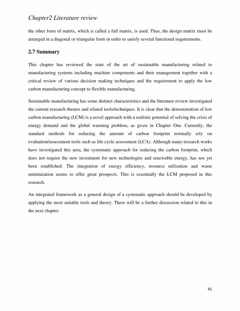
Chapter2 Literature review
41
the other form of matrix, which is called a full matrix, is used. Thus, the design matrix must be
arranged in a diagonal or triangular form in order to satisfy several functional requirements.
2.7 Summary
This chapter has reviewed the state of the art of sustainable manufacturing related to
manufacturing systems including machine components and their management together with a
critical review of various decision making techniques and the requirement to apply the low
carbon manufacturing concept to flexible manufacturing.
Sustainable manufacturing has some distinct characteristics and the literature review investigated
the current research themes and related tools/techniques. It is clear that the demonstration of low
carbon manufacturing (LCM) is a novel approach with a realistic potential of solving the crisis of
energy demand and the global warming problem, as given in Chapter One. Currently, the
standard methods for reducing the amount of carbon footprint normally rely on
evaluation/assessment tools such as life cycle assessment (LCA). Although many research works
have investigated this area, the systematic approach for reducing the carbon footprint, which
does not require the new investment for new technologies and renewable energy, has not yet
been established. The integration of energy efficiency, resource utilization and waste
minimization seems to offer great prospects. This is essentially the LCM proposed in this
research.
An integrated framework as a general design of a systematic approach should be developed by
applying the most suitable tools and theory. There will be a further discussion related to this in
the next chapter.
Chapter3 Research methodology
42
Chapter 3 Research methodology
3.1 Introduction
According to the literature review in the previous chapter, many research works on sustainable
manufacturing and environmental issues have been specifically paid attention to, including
evaluation, optimization, decision making and assessment. From this background, a systematic
method to implement low carbon manufacturing for real practice is very important. In this
chapter, all methodologies including experimental set-up, experimental design, prediction tool,
optimization tool and simulation tool are presented in a systematic way. This chapter also would
like to present the integration of different powerful tools in order to cope with energy efficiency,
resource utilization and waste minimization.
3.2 The scope of the research methodology
In this research, methodologies are divided into four stages as illustrated in Fig. 3.1: critical
review previous research related to attempt on low carbon manufacturing, development of low
carbon manufacturing concept, modeling of EREE-based low carbon manufacturing and
implementation. The details of each stage are described as follow:
(1) Critical review related research: previous research works especially on sustainable
manufacturing and energy efficiency manufacturing platform are critical reviewed in
order to investigate the existing sustainable manufacturing platform and knowledge gap
for developing low carbon manufacturing. This section is discussed in chapter 2.
(2) Development of low carbon manufacturing conception: information from previous
research works and requirements of contemporary regulations are gathered to formulate
characterization and theoretical model for low carbon manufacturing. In addition,
framework for different manufacturing levels is also proposed in this section according to
developed characterizations. This stage is discussed in chapter 4.
(3) Modelling of EREE-based low carbon manufacturing: the modelling is developed to
explain interaction between characterizations discussed in chapter 4 to gain low amount
of carbon emissions. The modelling is formulated in the form of matrix using Axiomatrix
Design discussed in chapter 2. The details of this stage are illustrated in chapter 5.
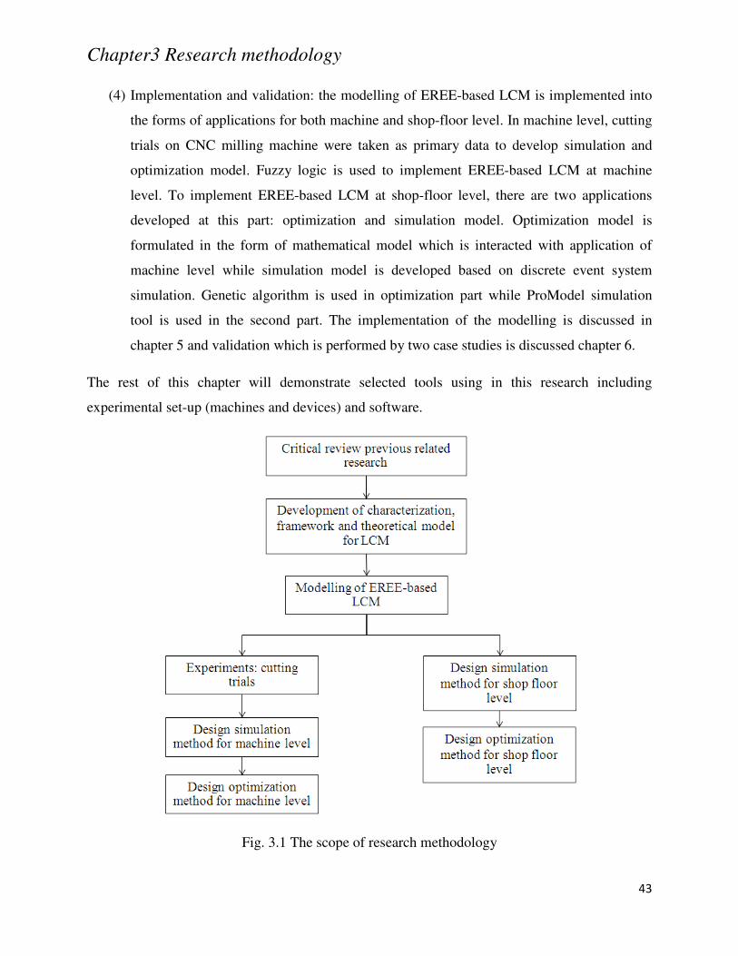
Chapter3 Research methodology
43
(4) Implementation and validation: the modelling of EREE-based LCM is implemented into
the forms of applications for both machine and shop-floor level. In machine level, cutting
trials on CNC milling machine were taken as primary data to develop simulation and
optimization model. Fuzzy logic is used to implement EREE-based LCM at machine
level. To implement EREE-based LCM at shop-floor level, there are two applications
developed at this part: optimization and simulation model. Optimization model is
formulated in the form of mathematical model which is interacted with application of
machine level while simulation model is developed based on discrete event system
simulation. Genetic algorithm is used in optimization part while ProModel simulation
tool is used in the second part. The implementation of the modelling is discussed in
chapter 5 and validation which is performed by two case studies is discussed chapter 6.
The rest of this chapter will demonstrate selected tools using in this research including
experimental set-up (machines and devices) and software.
Fig. 3.1 The scope of research methodology
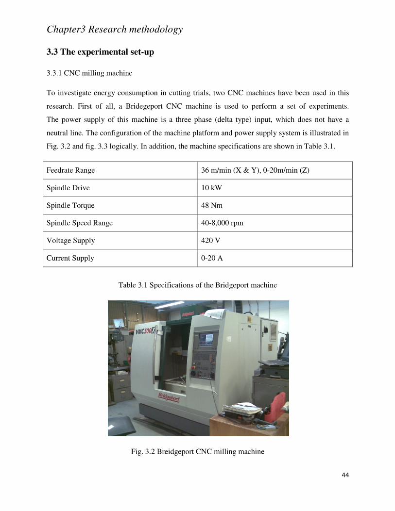
Chapter3 Research methodology
44
3.3 The experimental set-up
3.3.1 CNC milling machine
To investigate energy consumption in cutting trials, two CNC machines have been used in this
research. First of all, a Bridegeport CNC machine is used to perform a set of experiments.
The power supply of this machine is a three phase (delta type) input, which does not have a
neutral line. The configuration of the machine platform and power supply system is illustrated in
Fig. 3.2 and fig. 3.3 logically. In addition, the machine specifications are shown in Table 3.1.
Feedrate Range 36 m/min (X & Y), 0-20m/min (Z)
Spindle Drive 10 kW
Spindle Torque 48 Nm
Spindle Speed Range 40-8,000 rpm
Voltage Supply 420 V
Current Supply 0-20 A
Table 3.1 Specifications of the Bridgeport machine
Fig. 3.2 Breidgeport CNC milling machine
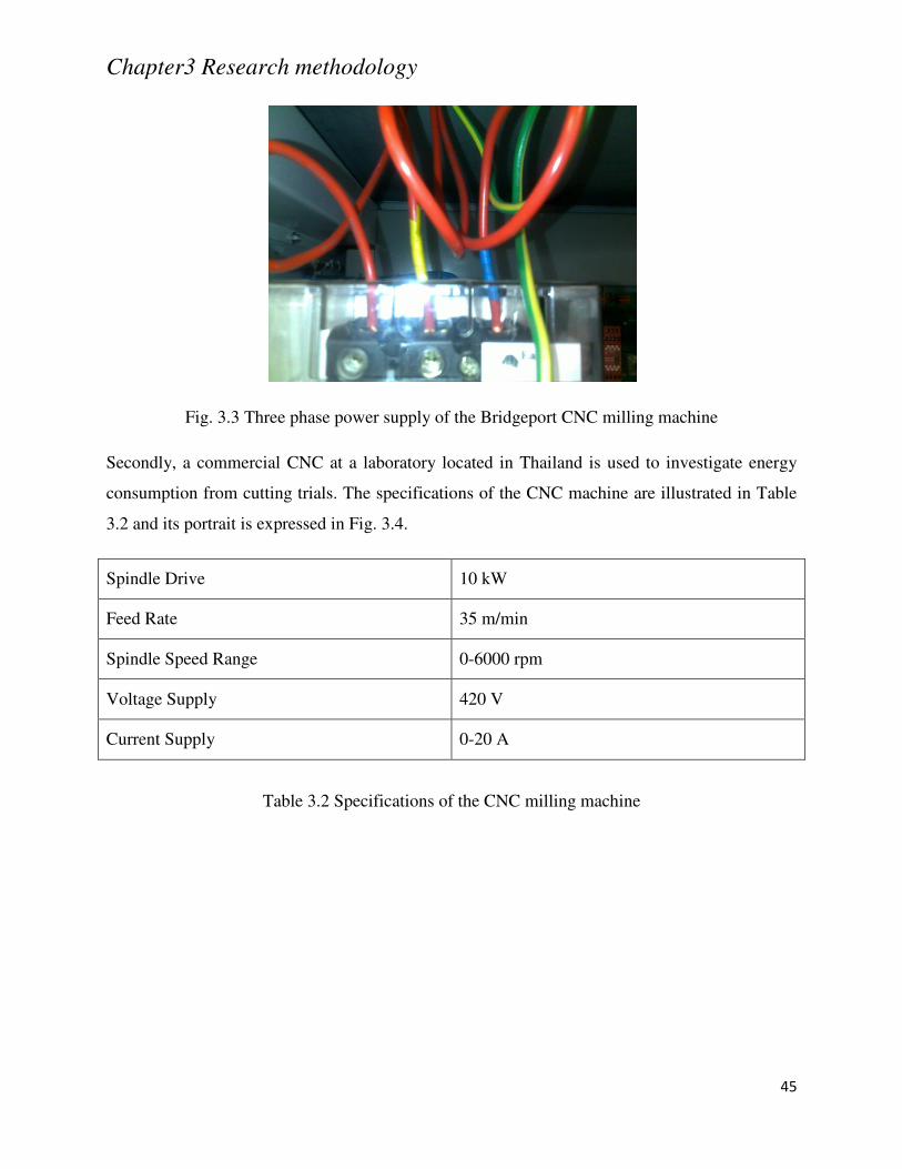
Chapter3 Research methodology
45
Fig. 3.3 Three phase power supply of the Bridgeport CNC milling machine
Secondly, a commercial CNC at a laboratory located in Thailand is used to investigate energy
consumption from cutting trials. The specifications of the CNC machine are illustrated in Table
3.2 and its portrait is expressed in Fig. 3.4.
Spindle Drive 10 kW
Feed Rate 35 m/min
Spindle Speed Range 0-6000 rpm
Voltage Supply 420 V
Current Supply 0-20 A
Table 3.2 Specifications of the CNC milling machine
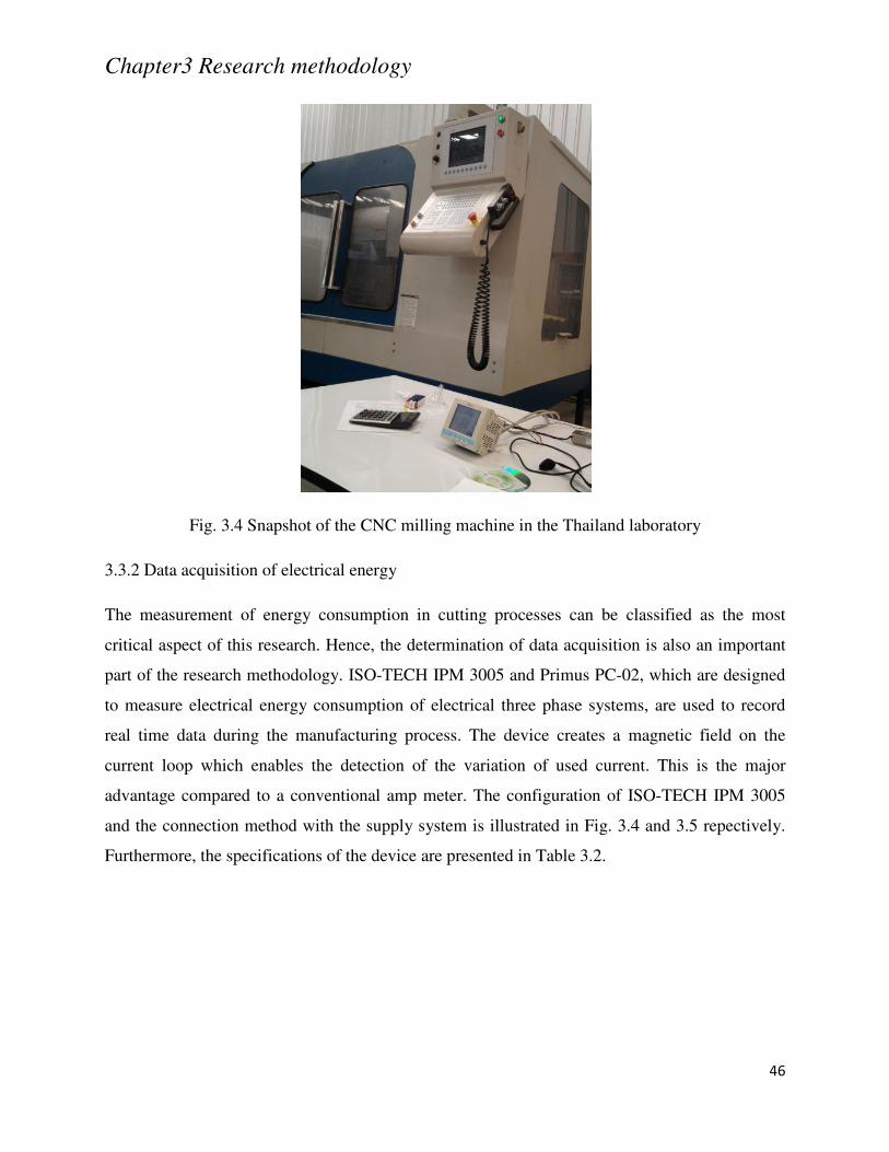
Chapter3 Research methodology
46
Fig. 3.4 Snapshot of the CNC milling machine in the Thailand laboratory
3.3.2 Data acquisition of electrical energy
The measurement of energy consumption in cutting processes can be classified as the most
critical aspect of this research. Hence, the determination of data acquisition is also an important
part of the research methodology. ISO-TECH IPM 3005 and Primus PC-02, which are designed
to measure electrical energy consumption of electrical three phase systems, are used to record
real time data during the manufacturing process. The device creates a magnetic field on the
current loop which enables the detection of the variation of used current. This is the major
advantage compared to a conventional amp meter. The configuration of ISO-TECH IPM 3005
and the connection method with the supply system is illustrated in Fig. 3.4 and 3.5 repectively.
Furthermore, the specifications of the device are presented in Table 3.2.
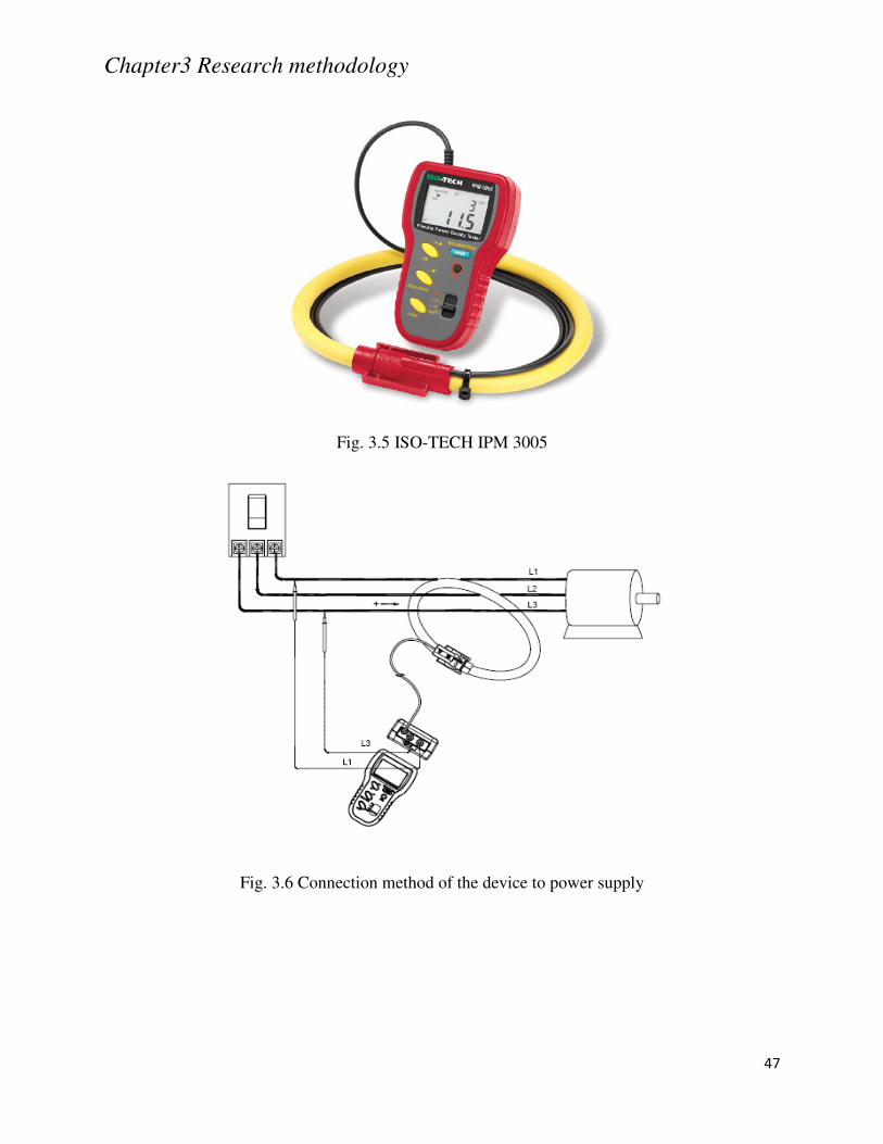
Chapter3 Research methodology
47
Fig. 3.5 ISO-TECH IPM 3005
Fig. 3.6 Connection method of the device to power supply
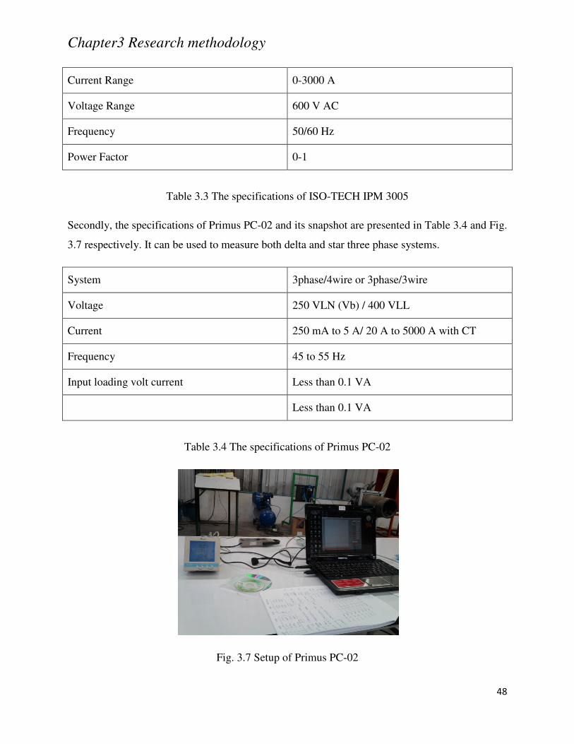
Chapter3 Research methodology
48
Current Range 0-3000 A
Voltage Range 600 V AC
Frequency 50/60 Hz
Power Factor 0-1
Table 3.3 The specifications of ISO-TECH IPM 3005
Secondly, the specifications of Primus PC-02 and its snapshot are presented in Table 3.4 and Fig.
3.7 respectively. It can be used to measure both delta and star three phase systems.
Table 3.4 The specifications of Primus PC-02
Fig. 3.7 Setup of Primus PC-02
System 3phase/4wire or 3phase/3wire
Voltage 250 VLN (Vb) / 400 VLL
Current 250 mA to 5 A/ 20 A to 5000 A with CT
Frequency 45 to 55 Hz
Input loading volt current Less than 0.1 VA
Less than 0.1 VA
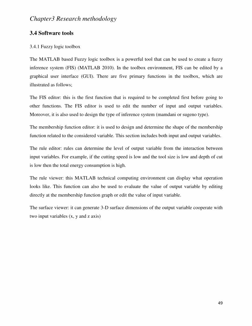
Chapter3 Research methodology
49
3.4 Software tools
3.4.1 Fuzzy logic toolbox
The MATLAB based Fuzzy logic toolbox is a powerful tool that can be used to create a fuzzy
inference system (FIS) (MATLAB 2010). In the toolbox environment, FIS can be edited by a
graphical user interface (GUI). There are five primary functions in the toolbox, which are
illustrated as follows;
The FIS editor: this is the first function that is required to be completed first before going to
other functions. The FIS editor is used to edit the number of input and output variables.
Moreover, it is also used to design the type of inference system (mamdani or sugeno type).
The membership function editor: it is used to design and determine the shape of the membership
function related to the considered variable. This section includes both input and output variables.
The rule editor: rules can determine the level of output variable from the interaction between
input variables. For example, if the cutting speed is low and the tool size is low and depth of cut
is low then the total energy consumption is high.
The rule viewer: this MATLAB technical computing environment can display what operation
looks like. This function can also be used to evaluate the value of output variable by editing
directly at the membership function graph or edit the value of input variable.
The surface viewer: it can generate 3-D surface dimensions of the output variable cooperate with
two input variables (x, y and z axis)
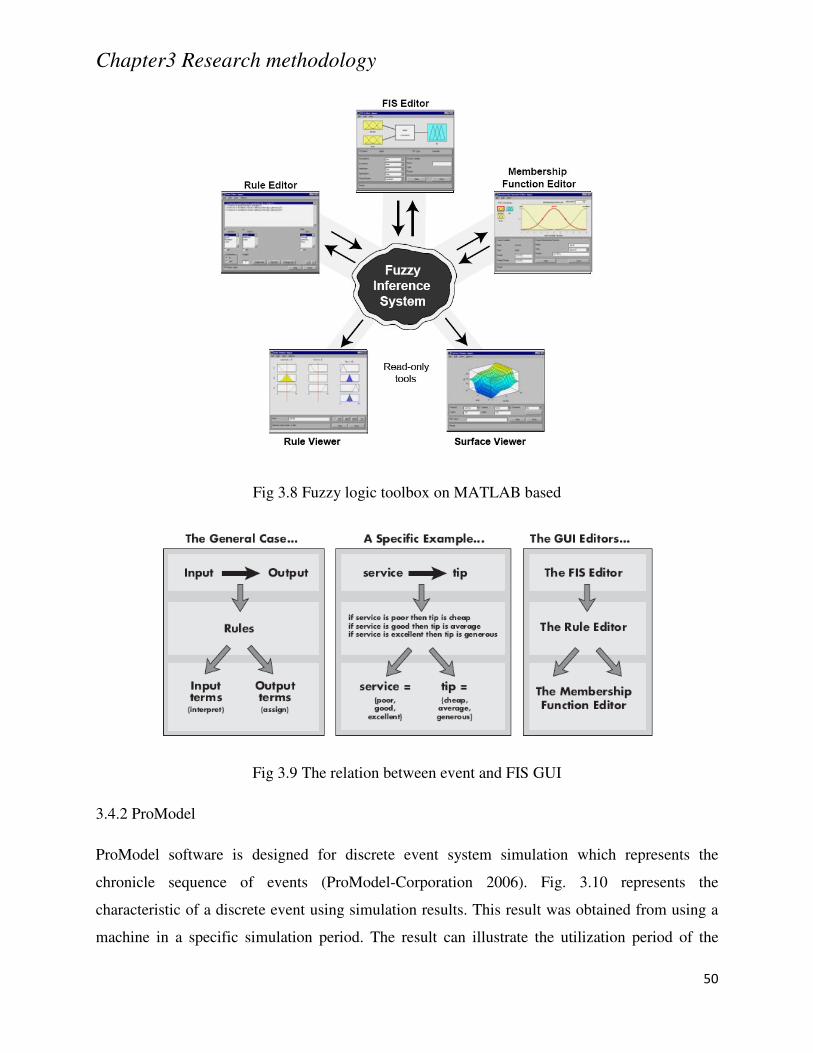
Chapter3 Research methodology
50
Fig 3.8 Fuzzy logic toolbox on MATLAB based
Fig 3.9 The relation between event and FIS GUI
3.4.2 ProModel
ProModel software is designed for discrete event system simulation which represents the
chronicle sequence of events (ProModel-Corporation 2006). Fig. 3.10 represents the
characteristic of a discrete event using simulation results. This result was obtained from using a
machine in a specific simulation period. The result can illustrate the utilization period of the
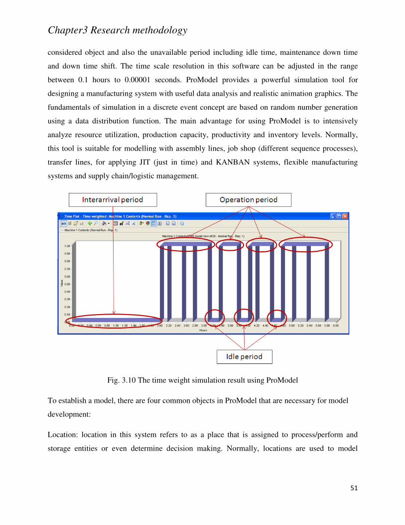
Chapter3 Research methodology
51
considered object and also the unavailable period including idle time, maintenance down time
and down time shift. The time scale resolution in this software can be adjusted in the range
between 0.1 hours to 0.00001 seconds. ProModel provides a powerful simulation tool for
designing a manufacturing system with useful data analysis and realistic animation graphics. The
fundamentals of simulation in a discrete event concept are based on random number generation
using a data distribution function. The main advantage for using ProModel is to intensively
analyze resource utilization, production capacity, productivity and inventory levels. Normally,
this tool is suitable for modelling with assembly lines, job shop (different sequence processes),
transfer lines, for applying JIT (just in time) and KANBAN systems, flexible manufacturing
systems and supply chain/logistic management.
Fig. 3.10 The time weight simulation result using ProModel
To establish a model, there are four common objects in ProModel that are necessary for model
development:
Location: location in this system refers to as a place that is assigned to process/perform and
storage entities or even determine decision making. Normally, locations are used to model
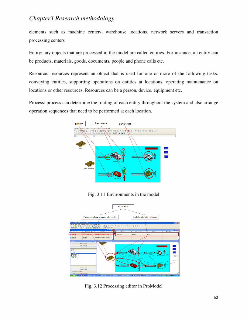
Chapter3 Research methodology
52
elements such as machine centers, warehouse locations, network servers and transaction
processing centers
Entity: any objects that are processed in the model are called entities. For instance, an entity can
be products, materials, goods, documents, people and phone calls etc.
Resource: resources represent an object that is used for one or more of the following tasks:
conveying entities, supporting operations on entities at locations, operating maintenance on
locations or other resources. Resources can be a person, device, equipment etc.
Process: process can determine the routing of each entity throughout the system and also arrange
operation sequences that need to be performed at each location.
Fig. 3.11 Environments in the model
Fig. 3.12 Processing editor in ProModel

Chapter3 Research methodology
53
Fig. 3.11 demonstrates important elements constructed in a flexible manufacturing model.
There are four types of machines (location) that are supported by operators (resource) to perform
four types of products (entity). The snapshot of processing editor in ProModel is illustrated in
Fig. 3.12, which is the same flexible manufacturing model that is presented in Fig. 3.11. This
example shows the processing environment in the waiting area for product type A. It has to be
waiting at this location (using a command to control this sequence) before determining which
machine should be used to perform (routing logic).
3.4.3 MATLAB based Genetic Algorithm toolbox
A genetic algorithm (GA) is one of the optimization methods that is used to solve both constraint
and unconstraint problems by using natural selection methodology (MATLAB 2010). Its main
algorithm is based on biological evolution by repeatedly modifying a population of individual
solutions. In every cycle, the algorithm randomly selects from the current population as parents
to generate children for the new generation by using cross over and mutation rules. Normally, the
modified iteration is terminated when either the maximum number of population generations has
been reached or the tolerance of fitness function value is satisfied by the optimized solution. In
addition, the solution returned from the algorithm might not be a global solution but just a local
solution when the iteration was terminated by the maximum population limit.
In this research, the genetic algorithm toolbox with MATLAB is used to solve the problem
constructed with objective function, constraints and range of variables (interested decision
variables). The mathematical formulation can be transformed into basic language in M-file
commands. In case of linear form problems, constraints can be arranged easily in the form of a
matrix in the command line. However, constraints are also required to transform into M-file as
well as objective function when the non-linear problem needs to be solved. The important
parameters that are determined before running the algorithm are illustrated as follow
[x fval] = ga(@fitnessfun, nvars, A, b, Aeq, beq, lb, ub, nonlcon, options)
Where
x: represents the final value of each decision variable that satisfies the terminated condition.
fval: represents the value of objective function using the value of optimized solution

Chapter3 Research methodology
54
@fitnessfun: represents the objective function (M-file)
nvars: number of design variables
A and b: used for creating matrix and vector for inequality constraints
Aeq and beq: used for creating matrix and vector for equality constraints
lb and ub: represent lower bound and upper bound of decision variable range
nonlcon: represents mathematical formulation of nonlinear constraint (M-file)
options: represents genetic algorithm set-up such as generation limit, time limit, tolerance of
constraint and tolerance of fitness function etc.
In Figs 3.13 and 3.14, the snapshots of objective function and nonlinear constraints creation on
M-file are presented respectively. These two screenshots are established based on a fuzzy integer
programming for a flexible manufacturing problem. Fig. 3.15 presents the snapshot of using a
genetic algorithm from the command line in MATLAB workspace.
Fig 3.13 Objective establishment in M-file
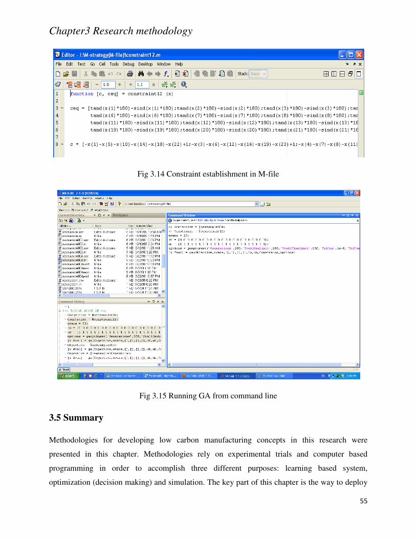
Chapter3 Research methodology
55
Fig 3.14 Constraint establishment in M-file
Fig 3.15 Running GA from command line
3.5 Summary
Methodologies for developing low carbon manufacturing concepts in this research were
presented in this chapter. Methodologies rely on experimental trials and computer based
programming in order to accomplish three different purposes: learning based system,
optimization (decision making) and simulation. The key part of this chapter is the way to deploy

Chapter3 Research methodology
56
different tools that have originally different theoretical backgrounds in a logical way, right place
and right purpose. Methodologies presented in this chapter are both related to machine level and
shopfloor level.
Chapter4 A framework for developing EREE-based LCM
57
Chapter 4 A framework for developing EREE-based LCM
4.1 Introduction
Due to the literature review in the chapter three, although the awareness on formulating low
carbon manufacturing concept has been mentioned as a timely topic, the systematic approach for
transforming the existing system into low carbon industry has not been robust defined. However,
many countries are now suffering the requirement from cooperation in carbon dioxide emissions
protocol in order to cope with global warming problem and also enhance sustainability. From the
national scale, it also leads to the smaller scale that uses carbon based energy such as industrial
sectors, companies and enterprises etc. to provide new methodologies/solutions that can satisfy
the target of carbon dioxide reduction in national scale. For this reason, the LCM must be able
not only to reduce the total amount of carbon dioxide emissions but also integrate the sustainable
ability in itself. This has important implications for the architecture of the framework and the
development of LCM.
Moreover, it is clear from the literature review that optimization techniques and waste reduction
methodologies such as lean manufacturing are taken in several researches in environmental and
sustainable areas. It has the potential to integrate these methodologies to develop initial LCM.
A more practical of combining essential approaches will be demonstrated in the following
sections in this chapter.
4.2 State of the Art
Recently, the term of sustainable manufacturing has been discussed across the value stream
(manufacturing process throughout supply chain) in order to make awareness of using energy
and resource more efficient and effective. On the other hand, this term can be used broadly for
environmental impact topics. Thus, the concept of low carbon manufacturing is emerging to
specifically reduce carbon footprint and energy consumption by applying the principle of
sustainable manufacturing while essential manufacturing performances (cost, quality and time)
can still be simultaneously achieved. However, a schism arises when exploring the strategic
framework, approaches, systematic implementation and application perspectives which are still
ambiguous. Many researchers have been investigating the methods for reducing carbon
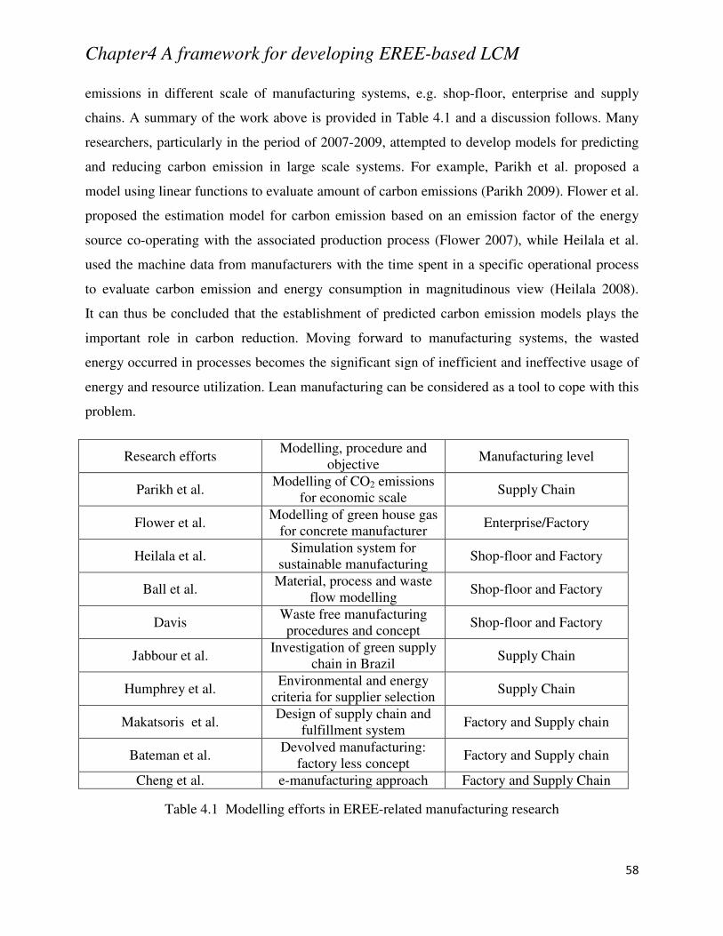
Chapter4 A framework for developing EREE-based LCM
58
emissions in different scale of manufacturing systems, e.g. shop-floor, enterprise and supply
chains. A summary of the work above is provided in Table 4.1 and a discussion follows. Many
researchers, particularly in the period of 2007-2009, attempted to develop models for predicting
and reducing carbon emission in large scale systems. For example, Parikh et al. proposed a
model using linear functions to evaluate amount of carbon emissions (Parikh 2009). Flower et al.
proposed the estimation model for carbon emission based on an emission factor of the energy
source co-operating with the associated production process (Flower 2007), while Heilala et al.
used the machine data from manufacturers with the time spent in a specific operational process
to evaluate carbon emission and energy consumption in magnitudinous view (Heilala 2008).
It can thus be concluded that the establishment of predicted carbon emission models plays the
important role in carbon reduction. Moving forward to manufacturing systems, the wasted
energy occurred in processes becomes the significant sign of inefficient and ineffective usage of
energy and resource utilization. Lean manufacturing can be considered as a tool to cope with this
problem.
Research efforts Modelling, procedure and
objective Manufacturing level
Parikh et al. Modelling of CO2 emissions
for economic scale Supply Chain
Flower et al. Modelling of green house gas
for concrete manufacturer Enterprise/Factory
Heilala et al. Simulation system for
sustainable manufacturing Shop-floor and Factory
Ball et al. Material, process and waste
flow modelling Shop-floor and Factory
Davis Waste free manufacturing procedures and concept
Shop-floor and Factory
Jabbour et al. Investigation of green supply
chain in Brazil Supply Chain
Humphrey et al. Environmental and energy
criteria for supplier selection Supply Chain
Makatsoris et al. Design of supply chain and
fulfillment system Factory and Supply chain
Bateman et al. Devolved manufacturing:
factory less concept Factory and Supply chain
Cheng et al. e-manufacturing approach Factory and Supply Chain
Table 4.1 Modelling efforts in EREE-related manufacturing research
Chapter4 A framework for developing EREE-based LCM
59
Additionally, it might not be sufficient for the whole enterprise to reduce carbon emissions and
energy consumptions by focusing only on manufacturing systems. Ball et al. proposed the
concept of utilizing energy and waste of the facility and utility by applying the waste from one
process to be used as an input to another process (Ball 2009). This can be combined with the
workplace organization method as presented by Davis et al. (Davis 1999). This concept
demonstrates the procedure to seek out waste that can be found in the organization to implement
waste free manufacturing. At the supply chain level, many researchers unveiled that most
industrial sectors and companies have not taken account of sustainable criteria and
environmental impact, which is meant inefficient energy wise on the value stream (Jabbour
2009). In the mean time, Humphreys et al. proposed the model integrated with environmental
and energy criteria for suppliers’ selection, which leads to the green supply chain (Humphreys
2003). In management of supply chains, Makatsoris et al. developed the model using e-
manufacturing to maximize production planning together with supply chains planning with the
real time system (Makatsoris 2004). Bateman et al. developed the concept of ‘factory less’ to
improve supply chains performance with less transportation using Devolved Manufacturing as an
approach (Bateman 2006). This concept can reduce the carbon emission from the value stream
network. Moreover, Cheng et al. suggested that the concept of extended supply chains network
performance using e-manufacturing has the high potential for success (Cheng 2008). From the
literatures having been critically reviewed, it can be concluded that the approach to reduce
carbon footprint and energy consumption is likely to play an important role in manufacturing
systems. However, the core framework and specific approach applicable to every level of
manufacturing operations have not been investigated systematically yet. The knowledge
gap needs to be fulfilled and implementation and application perspectives need to be investigated
and well understood.
4.2.1 Carbon Emissions Analysis
In the past decade, many countries have been conscious to develop the procedures for reducing
carbon emissions. Fan et al. (Fan 2007) have presented the model for prediction of carbon
dioxide (CO2) emissions based on the input of population, economy and urbanization. In 1996,
Golove and Schipper (Golove 1996) introduced the analysis of the tendency of energy
consumption which can cause CO2 emissions from manufacturing sectors based on the input of
Chapter4 A framework for developing EREE-based LCM
60
the gross domestic product (GDP) changed to economic output and process intensity. Although,
these methods have been developed to deal with the global warming problem from carbon
contents, the procedures to analyse is still focusing on the wide range and depending more on
economic factors such as GDP. The procedures for reducing CO2 emissions in manufacturing
systems and the associated manufacturing processes have not been introduced yet.
4.2.2 Operational Model
In the area of production research, most of the research focuses on the objective such as cost
minimization, quality assurance and the level of customer satisfaction as the objectives of the
process optimization according to Gungor and Gupta (1999) (Gungor 1999). Carbon emissions
and energy efficiency have never been a critical factor in operation optimization. However,
Mouzon et al. (Mouzon 2007) have developed the operational model by using the theory of
multi-objective mathematical programming in order to minimize energy consumption from
equipments in manufacturing system. In the operational model, the constraints are focusing on
completion time and total power per unit time. Even though, the production research for reducing
total energy consumption has been introduced at this time, the operational model for reducing
carbon contents from manufacturing processes need to be further developed.
4.2.3 Desktop and Micro Factory
The concepts of micro-factory and desktop machines for micro manufacturing purpose have been
explored in the wide range. For the definition and concepts of the micro-factory and desktop
machine, Yuichi (Okazaki 2004) explain it as small scale manufacturing systems which can
perform with higher throughput while resource utilization and energy consumption rate can be
reduced simultaneously. In addition, Mishima (Mishima 2006) suggests that the concept of
micro-factory and desktop machines should also concentrate on low heat generation and less
energy consumptions of the systems. It is concluded that the concept of desk-top and micro
factory can be applied to the LCM by reducing the unnecessary carbon contents from
manufacturing systems.
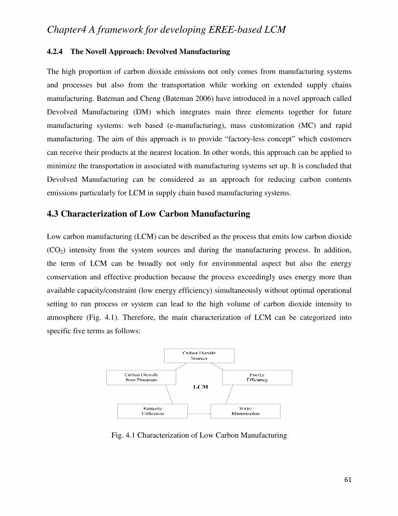
Chapter4 A framework for developing EREE-based LCM
61
4.2.4 The Novell Approach: Devolved Manufacturing
The high proportion of carbon dioxide emissions not only comes from manufacturing systems
and processes but also from the transportation while working on extended supply chains
manufacturing. Bateman and Cheng (Bateman 2006) have introduced in a novel approach called
Devolved Manufacturing (DM) which integrates main three elements together for future
manufacturing systems: web based (e-manufacturing), mass customization (MC) and rapid
manufacturing. The aim of this approach is to provide “factory-less concept” which customers
can receive their products at the nearest location. In other words, this approach can be applied to
minimize the transportation in associated with manufacturing systems set up. It is concluded that
Devolved Manufacturing can be considered as an approach for reducing carbon contents
emissions particularly for LCM in supply chain based manufacturing systems.
4.3 Characterization of Low Carbon Manufacturing
Low carbon manufacturing (LCM) can be described as the process that emits low carbon dioxide
(CO2) intensity from the system sources and during the manufacturing process. In addition,
the term of LCM can be broadly not only for environmental aspect but also the energy
conservation and effective production because the process exceedingly uses energy more than
available capacity/constraint (low energy efficiency) simultaneously without optimal operational
setting to run process or system can lead to the high volume of carbon dioxide intensity to
atmosphere (Fig. 4.1). Therefore, the main characterization of LCM can be categorized into
specific five terms as follows:
Fig. 4.1 Characterization of Low Carbon Manufacturing
Chapter4 A framework for developing EREE-based LCM
62
(1) Low carbon dioxide from source: currently, almost all equipment and machines in modern
industry use electricity as a main energy to operate if machines or equipment can be adjusted
or improved to use less energy, the carbon dioxide intensity from the machines and
equipment sources will be reduced because the conventional electricity generation consumes
fossil fuel which is the source of carbon dioxide.
(2) Low carbon dioxide from process: this can be referred to the process that directly generates
carbon intensity to the atmosphere e.g. chemical process using crude oil or fossil fuel.
The amount of carbon intensity can be reduced if the optimal process parameters can be
determined when energy consumption rate or carbon emissions are considered as an
objective to be minimized.
(3) Energy efficiency: energy efficiency can be explained as a percentage of output of energy
from process (in watt or joules) divided by the input amount of energy (Edwards 2012).
Hence, this parameter in LCM concept should be higher than conventional industrial
processes.
(4) Waste minimization: This term can be meant as how waste can be dislodged or minimized
according to the reference (Mulholland 2001). If the third criteria above are categorized into
carbon dioxide emissions due to machines and equipment, the term ‘waste’ represents
undesired manufacturing wastes that affect on the total carbon emissions. For example,
many wastes can appear in the turbulent manufacturing process: idle time, waiting time and
queuing time etc. Therefore, the optimal solution and algorithm (for example, optimal time
to run machines and equipment which can conform to operational constraint) for the
manufacturing process should be installed into LCM in order to minimize waste energy and
thus carbon dioxide emissions.
(5) Resource utilization: Sivasubramanian et al. (Sivasubramanian 2003) described that
resource utilization in today industry can be typically observed from raw material usage and
queue/waiting time in the process and priority rule in the process chain. These factors can
become as constraints in problem formulation in order to create optimal production
algorithm. The percent of carbon contents can be reduced when percent of resource
utilizations are increased because unnecessary energy for CO2 emissions is also reduced.
Chapter4 A framework for developing EREE-based LCM
63
4.4 EREE-Based LCM: Conception and a Framework
According to the characterization of low carbon manufacturing, energy efficiency, resource
utilization and waste minimization are the key goals for realizing low carbon manufacturing and
consequently essential for its conception and quantitative analysis and modelling (E-R-W-C
modelling). The key constituents as formulated for the conception and framework are presented
in Table 4.2, in the format of a matrix highlighting the manufacturing levels (column) against
their individual characterizations (row). In the matrix, each cell represents the possible solution
for a specific manufacturing level to successfully complete relevant characterization.
For example, the matrix cell 1-1 represents recommended methods for the machine/process level
to achieve energy efficiency. The descriptions of proposed potential solutions for each
manufacturing level are further discussed in the rest of this section. Fig. 4.2 further illustrates
intricate relationships among the constituents of EREE-based LCM, which also demonstrates the
LCM outcomes are not only focused on the conventional manufacturing performance but also
sustainability and low carbon footprint.
Machine/Process: Most machines and processes consume energy in differential ways due to
their components and parts built with and procedures of the processes. Evaluation of energy
consumption from the machine/process is the essential part of studying the machine energy
efficiency/effectiveness. It is difficult to predict energy consumption from the process involving
multiple parameters setting such as cutting speed, depth of cut, feed rate, using cooling and
lubrication, etc. Therefore, the energy consumption modelling for the machine/process must be
carefully undertaken and laborious.
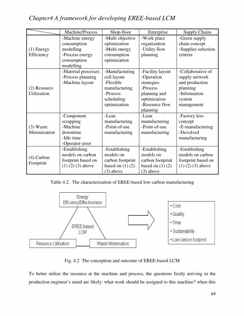
Chapter4 A framework for developing EREE-based LCM
64
Machine/Process Shop-floor Enterprise Supply Chains
(1) Energy Efficiency
-Machine energy consumption modelling -Process energy consumption modelling
-Multi objective optimization -Multi energy consumption optimization
-Work place organization -Utility flow planning
-Green supply chain concept -Supplier selection criteria
(2) Resource Utilization
-Material processes -Process planning -Machine layout
-Manufacturing cell layout -Flexible manufacturing -Process scheduling optimization
-Facility layout -Operation strategies -Process planning and optimization -Resource flow planning
-Collaborative of supply network and production planning -Information system management
(3) Waste Minimization
-Component scrapping -Machine downtime -Idle time -Operator error
-Lean manufacturing -Point-of-use manufacturing
-Lean manufacturing -Point-of-use manufacturing
-Factory less concept -E-manufacturing -Devolved manufacturing
(4) Carbon Footprint
-Establishing models on carbon footprint based on (1) (2) (3) above
-Establishing models on carbon footprint based on (1) (2) (3) above
-Establishing models on carbon footprint based on (1) (2) (3) above
-Establishing models on carbon footprint based on (1) (2) (3) above
Table 4.2. The characterization of EREE-based low carbon manufacturing
Fig. 4.2 The conception and outcome of EREE-based LCM
To better utilize the resource at the machine and process, the questions firstly arriving in the
production engineer’s mind are likely: what work should be assigned to this machine? when this
Chapter4 A framework for developing EREE-based LCM
65
machine should be started and stopped? where this machine should be located? All of the
question must be well attempted in order to maximize the machine’s utilisation for and in the
production process. To comply this step, the machine/process utilization must be co-operated
with energy consumption modelling so as to maximize the utilization and minimize the energy
consumption, and eliminate the waste in the machine and process. The typical wastes on a
machine come from components scrapping, machine down time, idle time and operator errors.
These wastes may cause imperfect machine/process conditions which again lead to undesired
energy and resource efficiency and effectiveness.
Shop-floor: This level refers to the floor of the workshop where technicians and engineers work
on the machine and manufacturing cell. In order to make energy efficient for shop-floor,
the model for predicting energy consumption is a key of success at this stage as well as shop-
floor level. However, the complexity arises when there are many machines to be involved (many
energy consumption models). In addition, the solution can be more complex when the production
objectives include not only energy consumption but also quality, time and cost. Therefore, the
multi objective optimisation method can be appropriate solution. The value of energy
consumption can compromise with other production performance e.g. minimizing energy
consumption and maximizing profit. Moving forward to resource utilisation, layout/position for
machines in shop floor might be an essential issue because of the complexity in process
planning. When machines/processes with same specific function are categorized in the same
location, it could be more convenience for process planning with maximized utilisation of each
machine/process. Thus, the principle of manufacturing cell layout and flexible manufacturing
can be applied to cope with this problem. These concepts must be combined with multi objective
optimisation including energy consumption model while to optimize the process scheduling.
As a result, the requirement of resource utilisation for the machine/process can be provided at
this stage. Furthermore, the conditions of the machine/process are also important for the shop-
floor (manufacturing cell). Lean manufacturing, therefore, can be applied to eliminate
unnecessary waste at shop-floor. Maintenance system can play an important role in this concept
because when shop-floor reliability improves, it can reflex in reduction of each machine/process
down time and component scrapping. Finally, the method of carbon footprint modelling based on
E-R-W-C can be applied just same as that for the machine/process level.
Chapter4 A framework for developing EREE-based LCM
66
Enterprise: There are many departments/sections in a manufacturing enterprise which can be
implied to many kinds of processes and functions occurred in the enterprise. On the other hand,
this means the complexity in evaluation of energy consumption at this stage due to the different
kinds of consumed energy (electricity, fossil fuel, resources, etc.). Hence, the concept of
workplace organization is suitable because the enterprise can seek out what kind of wastes
occurring from the specific area, then the concept of utility flow planning is used together to
efficiently consume energy at each department/section of the enterprise. When energy
requirement is determined in large scale, master process planning, which can be referred as
master production planning (MPS), is involved together to likely make resource planning
comprehensively. With effective process planning, the production manager can provide
operation strategies which can compromise between customer demands and available energy
requirement. This strategy also performs as the top-down process to shop-floor level because
each manufacturing cell receives work order after operation strategy was finished. To realize
energy consumption reduction for the enterprise, the concept of lean manufacturing can also be
used at this level as well as at shop-floor level. Taking account of inventory management,
the concept of making to order is not just for warehouse control but it can also reduce the waste
in terms of energy and resource when demand was changed. For carbon footprint modelling,
E-R-W-C method can be applied same as the previous two levels.
Supply Chain: Nowadays, the role of supply chains has highly impact on the whole value
stream in the competitive marketplace. The supplier selection becomes the successive key for an
enterprise to fulfil enterprise supply chain network. In order to make effective value stream, most
enterprises determine their supply chains based the conventional supplier performance,
e.g. delivery quality, cost and response time. However, the total performance of supply chain
network might not be sufficient for the contemporary manufacturing system due to the lack of
energy and environmental concern. On the other hand, it could be implied that the supply
network could have the effectiveness of quality, cost and delivery but the energy and
environmental inefficiency. Hence, the concept of green supply chain has high potential to be a
feasible solution at this stage. The criteria of supplier selection must have insertion of energy
concern in itself with the questions: how much the energy consumption is in the production
process? does the company have energy policy support? how does the company process wastes
from the production line? As a result, the total energy effectiveness of value stream can be
Chapter4 A framework for developing EREE-based LCM
67
improved by applying the new method of supplier selection. However, the completion of low
carbon manufacturing for supply chain level might be imperfect because of ineffective resource
utilisation. This could be meant that the poorly organized supply chain network between
suppliers and manufacturers can lead to waste of energy and resource including over production
process and unnecessary transportation, etc. Therefore, the effective information system
management is very important to create effective collaboration between supply network and
production planning by using e-manufacturing. With this method, the planning between suppliers
and manufacturers is optimized in light of the real time response of interactive e-manufacturing
system so as to maximize of resource utilisation with elimination of unnecessary waste energy.
In addition, the advantage of e-manufacturing is not only for supply chain resource utilisation but
also waste minimisation. The potential to complete this part with e-manufacturing is using
‘factory less’ concept or Devolved Manufacturing as a tool. The carbon emission from value
stream is likely decreased by combining we-based technology, mass customization and rapid
manufacturing, which may lead to the innovative manufacturing being carried out at the
customer’s door step in a rapid and EREE-oriented manner. This may further lead to point-of-use
manufacturing by using mobile smart machines or ‘factory box’, which possibly means some
modes of sustainable manufacturing in EREE context.
4.5 LCM theoretical model
According to the literature review in Chapter 2, it is obvious that the methodology for carbon
dioxide emissions evaluation and assessment is very essential as initial fundamental for LCM.
Optimization tools/techniques is also required to provide the effective operation when the firms
need to transform their existing system to be LCM environment. In addition, the elimination of
waste from manufacturing processes has been broadly investigated by many researchers in term
of sustainable development and environmental concern. Therefore, the theoretical model for
LCM shall compass three kinds of element, i.e. carbon dioxide emissions evaluation,
optimization methods and waste reduction methodologies, as shown in Fig. 4.3, which are also
described in details in the sub-sections below. Moreover, the theoretical model can be in various
such as mathematical modelling and simulation model.
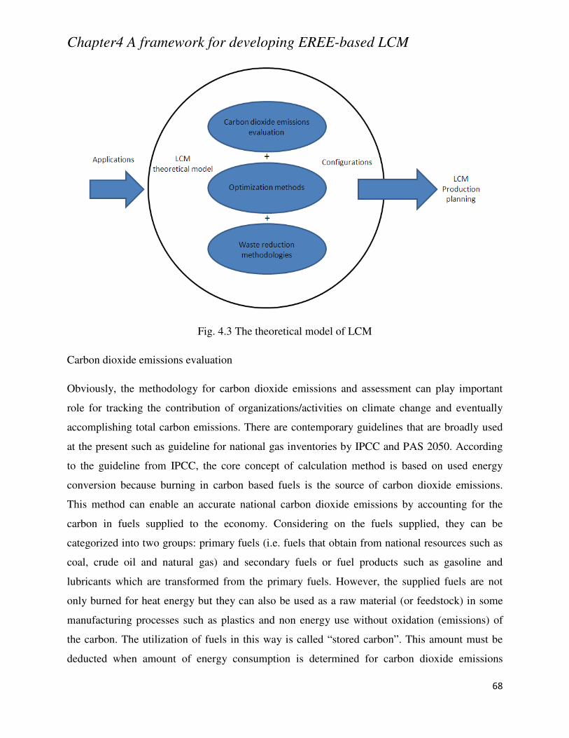
Chapter4 A framework for developing EREE-based LCM
68
Fig. 4.3 The theoretical model of LCM
Carbon dioxide emissions evaluation
Obviously, the methodology for carbon dioxide emissions and assessment can play important
role for tracking the contribution of organizations/activities on climate change and eventually
accomplishing total carbon emissions. There are contemporary guidelines that are broadly used
at the present such as guideline for national gas inventories by IPCC and PAS 2050. According
to the guideline from IPCC, the core concept of calculation method is based on used energy
conversion because burning in carbon based fuels is the source of carbon dioxide emissions.
This method can enable an accurate national carbon dioxide emissions by accounting for the
carbon in fuels supplied to the economy. Considering on the fuels supplied, they can be
categorized into two groups: primary fuels (i.e. fuels that obtain from national resources such as
coal, crude oil and natural gas) and secondary fuels or fuel products such as gasoline and
lubricants which are transformed from the primary fuels. However, the supplied fuels are not
only burned for heat energy but they can also be used as a raw material (or feedstock) in some
manufacturing processes such as plastics and non energy use without oxidation (emissions) of
the carbon. The utilization of fuels in this way is called “stored carbon”. This amount must be
deducted when amount of energy consumption is determined for carbon dioxide emissions
Chapter4 A framework for developing EREE-based LCM
69
calculation. Thus, IPCC suggests an initial approach for carbon dioxide emissions calculation
into six steps as follows
(1) Estimate apparent fuel combustion in original units
(2) Convert to a common energy unit
(3) Multiply by emission factors to compute the carbon content
(4) Compute carbon store
(5) Correct for carbon unoxidised
(6) Convert carbon oxidized to CO2 emissions
In PAS2050, it is also designed as an assistant guideline for carbon dioxide emissions
assessment. It main concept depends on analyzing of process chains/sequences.
Each process/activity must be determined whether there is carbon based fuels/energy involved in
the considered process/activity or not. Then, then amount of fuel/energy is multiplied by the
related coefficient. This can be implied that the main procedure of PAS 2050 and the guideline
from IPCC are identical but PAS 2050 is more suitable for enterprise/systems level while the
guideline from IPCC is suitable for national (large scale) level.
However, the schism arises when the well design and planning for supporting low carbon is
required. Referring to the literature review, many researchers have been trying to develop
methodologies and models which are not only just for assessment but also supports decision
making in term of simulation and predictability. In machine based manufacturing, the
systematical methodology that can evaluate the amount of energy consumption regarding to
machining condition set-up is essentially required according to literature reviews. It would be
rather to predict and simulate the amount of energy consumption with reliable and high precision
results before performing cutting process than only applying assessment at the end of the
process. Therefore, it is very essential to involve carbon dioxide emissions evaluation as one
element in the LCM theoretical model. The evaluation method must be developed by extending
from the conventional carbon dioxide emissions assessment/calculation.
Optimization methods
According to the literature review in Chapter2, various optimization techniques have been
applied into sustainable and environmental problem to provide the optimal solution. Normally,
Chapter4 A framework for developing EREE-based LCM
70
there are two main types of optimization methodologies with their unique advantages.
Their applications are determined based on the type/level of problem definition. Optimization
methods can return the best solution that can satisfy requirement of objective functions and
problem constraints. Therefore, it is very essential to involve optimization methods as one
element of LCM theoretical model.
Multi objective decision making (MODM) are naturally formulated in the form of mathematical
modelling regarding to problem descriptions. The structure of mathematical is constructed by
three parts: objective functions, problem constraints and range of decision variables. In objective
and constraint parts, the formulation can be established as linear and non linear equation while
the final part defines type and boundary of decision variables. Types of decision variable can be
both real or integer. The advantage of using MODM to cope optimization problem is capability
in solving complex problem. At the present, there are various methods of searching algorithm
that enable run time process to reach convergence point faster and easier such as genetic and
direct search algorithms. However, there can be a major problem from optimization procedure
due to searching criteria. Optimization algorithm may return global or local result. In other word,
global result is referred to the true optimal result while local result represents dummy result.
Therefore, the decision maker must always be aware in reliable of result from optimization
method because it can affect on all three elements (energy efficiency, resource utilization and
waste minimization) to achieve LCM.
Multi attribute decision making (MADM) is widely used when there are set of data/information
and objectives/goals to be determined. Most of MADM calculating process normalizes all data
due to their own reference methodology and objectives/goals requirement. The set of value
transformed by normalization method can be compared to select the best solution. MADM is not
complicate for the decision maker by its natural behavior (mathematical modelling is not
required to formulated). In addition, all feasible solutions are predetermined. It can be, in other
words, implied that the performances of possible solution are ordered due to the normalized
value. However, the application of MADM might not be flexible as MODM because the
selection of optimal solution using MADM can perform only on the available data/information
while MODM can define the boundary/range of decision variables.
Chapter4 A framework for developing EREE-based LCM
71
Waste reduction methodologies
As described in characterization of LCM, there are many types of waste that affect on the total
carbon emissions from manufacturing processes. Thus, it is very essential to define waste
reduction methodologies as one element of LCM theoretical model because even effective
carbon dioxide emission evaluation and optimization techniques are successful implemented into
production planning, it is still difficult to prevent undesired wastes from the real situation/process
running. There could be fluctuation in the expected results from evaluation and optimization
methods. On the other hand, it can be referred that the true LCM strategy cannot be
accomplished without the effective waste reduction methodologies. According to possible wastes
that can occur in manufacturing processes, the most important variable associated between
wastes and total carbon emissions is time. Thus, time based simulation could be a possible
solution to eliminate undesired wastes such as idle time, resource utilization and maintenance
down time etc.
4.6 Implementation of LCM at Enterprise and Supply Chains Level
Three implementations have been explored at Brunel University for LCM. The configuration of
implementation of LCM is shown in Fig. 4.4.
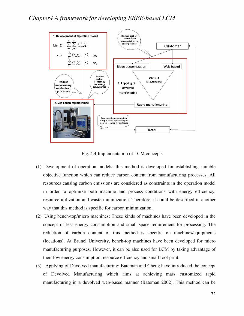
Chapter4 A framework for developing EREE-based LCM
72
Fig. 4.4 Implementation of LCM concepts
(1) Development of operation models: this method is developed for establishing suitable
objective function which can reduce carbon content from manufacturing processes. All
resources causing carbon emissions are considered as constraints in the operation model
in order to optimize both machine and process conditions with energy efficiency,
resource utilization and waste minimization. Therefore, it could be described in another
way that this method is specific for carbon minimization.
(2) Using bench-top/micro machines: These kinds of machines have been developed in the
concept of less energy consumption and small space requirement for processing. The
reduction of carbon content of this method is specific on machines/equipments
(locations). At Brunel University, bench-top machines have been developed for micro
manufacturing purposes. However, it can be also used for LCM by taking advantage of
their low energy consumption, resource efficiency and small foot print.
(3) Applying of Devolved manufacturing: Bateman and Cheng have introduced the concept
of Devolved Manufacturing which aims at achieving mass customized rapid
manufacturing in a devolved web-based manner (Bateman 2002). This method can be
Chapter4 A framework for developing EREE-based LCM
73
applied to the concept of LCM by minimizing carbon emission from make to order
product (upstream) by customizing product via Internet-based instead through the nearest
location (downstream) to pick-up finished goods (less transportation, less fossil fuel
burning). It can be explained in another words that this approach is focused on reducing
carbon emission from supply network.
4.7 Implementation of LCM at Machine and Shop-Floor Level
In this section, the application and implementation for EREE-based LCM conception and
framework are explored and presented. However, the work presented is focused on two
manufacturing levels: the machine/process and shop-floor level as the research project and
interests concerned. The previous section covers with the approaches cooperating with the
characterisation for low carbon manufacturing on different manufacturing level and then the
modelling, optimisation and simulation method are used as selected tools. In Figs 4.5 and 4.6,
the procedure is illustrated to establish the machine/process energy consumption modelling with
the well-design experimental measurement and testing for evaluating and validating the models.
In this research, the CNC based machining is carried out as on test workpieces to assess the
machine energy consumption and mapping in comparsion with modelling and simulation
predictions. The experiment was undertaken on cutting trial with different machining conditions
(cutting speed, depth of cut, tool size) and then collecting energy consumption data computer
acquitted via the power logger device. After data from the power logger was analysed,
the energy consumption model is created by using fuzzy inference system (FIS) as the AI tool
base (mamdani and sugeno type). In addition, sugeno type is used for energy consumption
prediction while mamdani type is used for optimization. The MATLAB GUI is used to create
user interface for user friendly purpose at this stage.
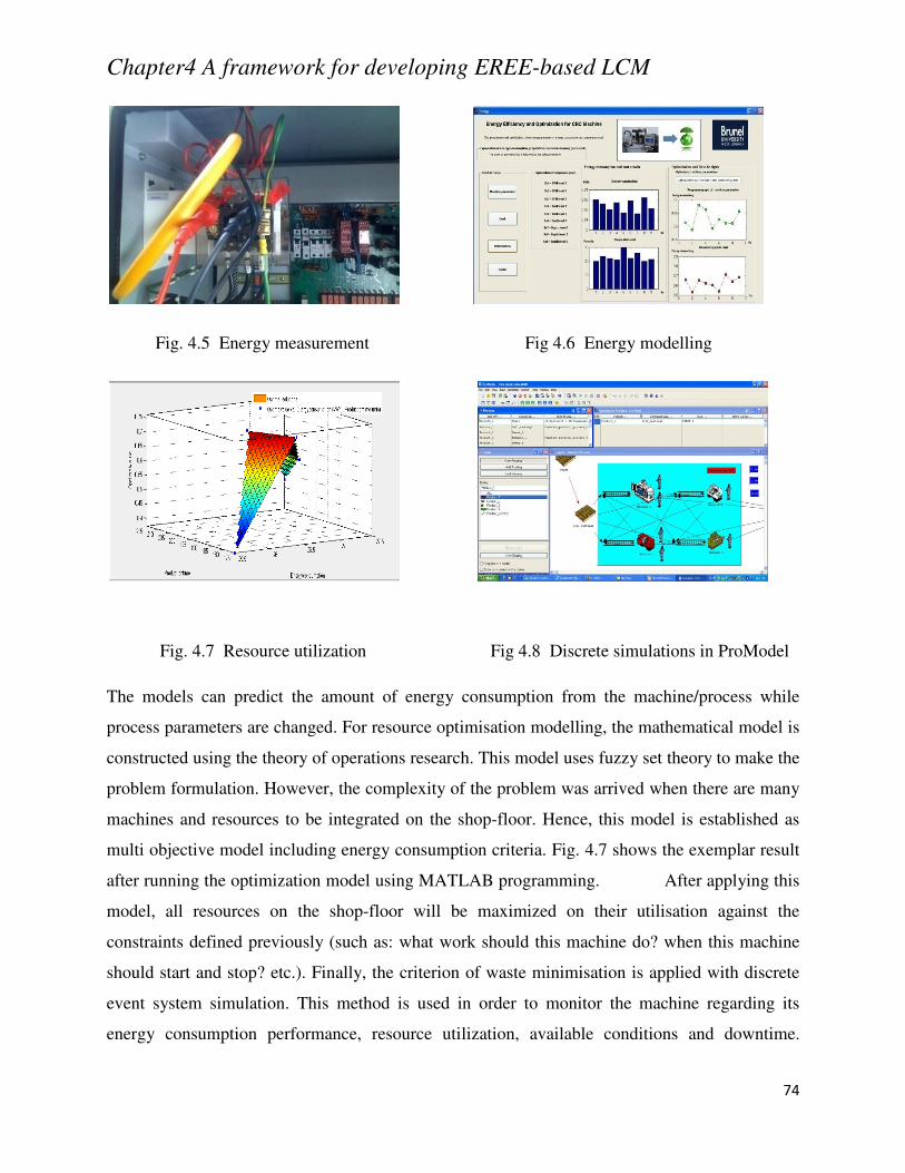
Chapter4 A framework for developing EREE-based LCM
74
Fig. 4.5 Energy measurement Fig 4.6 Energy modelling
Fig. 4.7 Resource utilization Fig 4.8 Discrete simulations in ProModel
The models can predict the amount of energy consumption from the machine/process while
process parameters are changed. For resource optimisation modelling, the mathematical model is
constructed using the theory of operations research. This model uses fuzzy set theory to make the
problem formulation. However, the complexity of the problem was arrived when there are many
machines and resources to be integrated on the shop-floor. Hence, this model is established as
multi objective model including energy consumption criteria. Fig. 4.7 shows the exemplar result
after running the optimization model using MATLAB programming. After applying this
model, all resources on the shop-floor will be maximized on their utilisation against the
constraints defined previously (such as: what work should this machine do? when this machine
should start and stop? etc.). Finally, the criterion of waste minimisation is applied with discrete
event system simulation. This method is used in order to monitor the machine regarding its
energy consumption performance, resource utilization, available conditions and downtime.
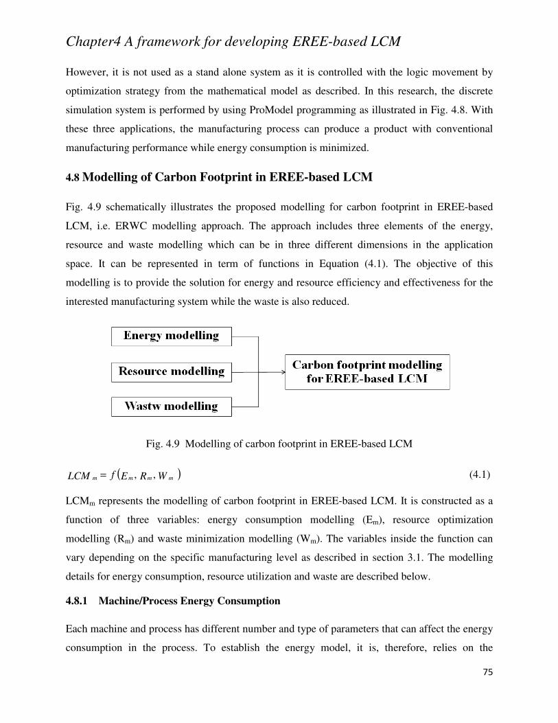
Chapter4 A framework for developing EREE-based LCM
75
However, it is not used as a stand alone system as it is controlled with the logic movement by
optimization strategy from the mathematical model as described. In this research, the discrete
simulation system is performed by using ProModel programming as illustrated in Fig. 4.8. With
these three applications, the manufacturing process can produce a product with conventional
manufacturing performance while energy consumption is minimized.
4.8 Modelling of Carbon Footprint in EREE-based LCM
Fig. 4.9 schematically illustrates the proposed modelling for carbon footprint in EREE-based
LCM, i.e. ERWC modelling approach. The approach includes three elements of the energy,
resource and waste modelling which can be in three different dimensions in the application
space. It can be represented in term of functions in Equation (4.1). The objective of this
modelling is to provide the solution for energy and resource efficiency and effectiveness for the
interested manufacturing system while the waste is also reduced.
Fig. 4.9 Modelling of carbon footprint in EREE-based LCM
( )WREfLCM mmmm ,,= (4.1)
LCMm represents the modelling of carbon footprint in EREE-based LCM. It is constructed as a
function of three variables: energy consumption modelling (Em), resource optimization
modelling (Rm) and waste minimization modelling (Wm). The variables inside the function can
vary depending on the specific manufacturing level as described in section 3.1. The modelling
details for energy consumption, resource utilization and waste are described below.
4.8.1 Machine/Process Energy Consumption
Each machine and process has different number and type of parameters that can affect the energy
consumption in the process. To establish the energy model, it is, therefore, relies on the
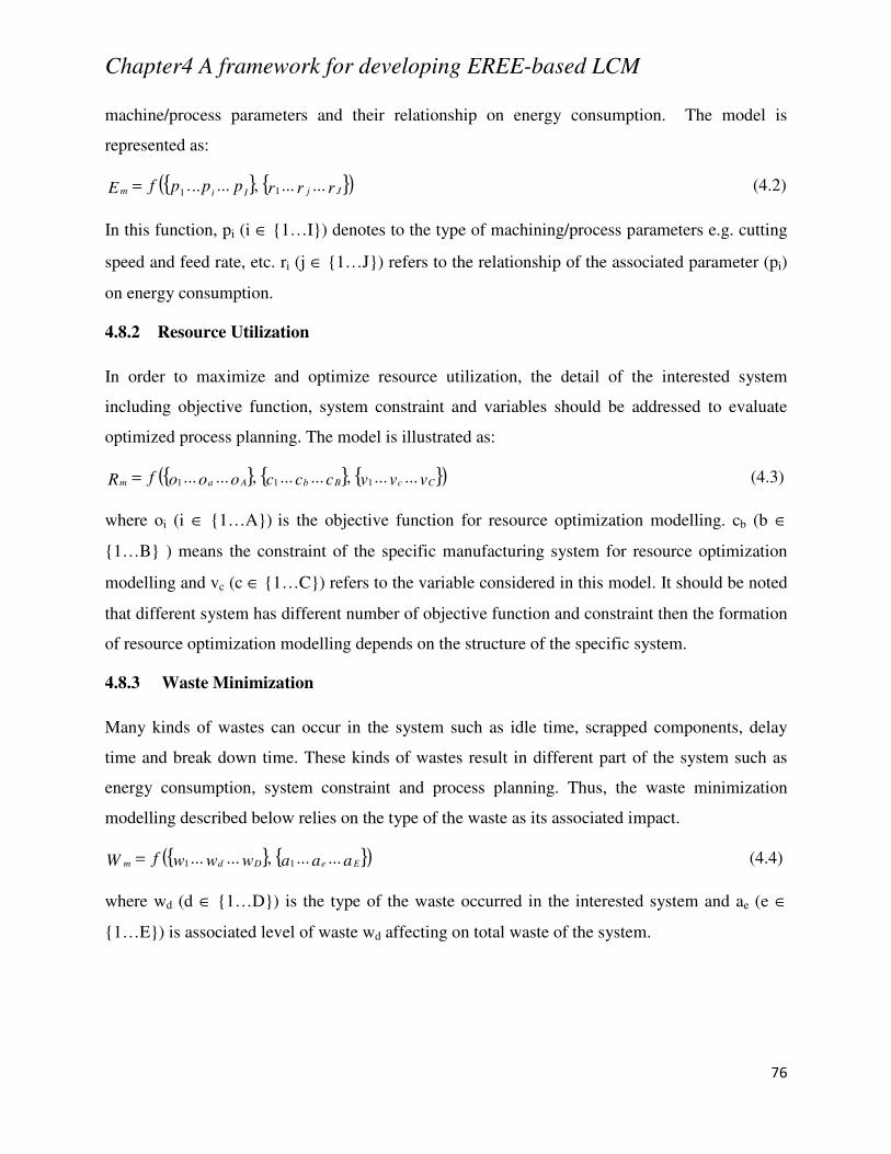
Chapter4 A framework for developing EREE-based LCM
76
machine/process parameters and their relationship on energy consumption. The model is
represented as:
( )rrrpppfE JjIim ......,...... 11= (4.2)
In this function, pi (i ∈ 1…I) denotes to the type of machining/process parameters e.g. cutting
speed and feed rate, etc. ri (j ∈ 1…J) refers to the relationship of the associated parameter (pi)
on energy consumption.
4.8.2 Resource Utilization
In order to maximize and optimize resource utilization, the detail of the interested system
including objective function, system constraint and variables should be addressed to evaluate
optimized process planning. The model is illustrated as:
( )vvvcccooofR CcBbAam ......,......,...... 111= (4.3)
where oi (i ∈ 1…A) is the objective function for resource optimization modelling. cb (b ∈
1…B ) means the constraint of the specific manufacturing system for resource optimization
modelling and vc (c ∈ 1…C) refers to the variable considered in this model. It should be noted
that different system has different number of objective function and constraint then the formation
of resource optimization modelling depends on the structure of the specific system.
4.8.3 Waste Minimization
Many kinds of wastes can occur in the system such as idle time, scrapped components, delay
time and break down time. These kinds of wastes result in different part of the system such as
energy consumption, system constraint and process planning. Thus, the waste minimization
modelling described below relies on the type of the waste as its associated impact.
( )aaawwwfW EeDdm ......,...... 11= (4.4)
where wd (d ∈ 1…D) is the type of the waste occurred in the interested system and ae (e ∈
1…E) is associated level of waste wd affecting on total waste of the system.
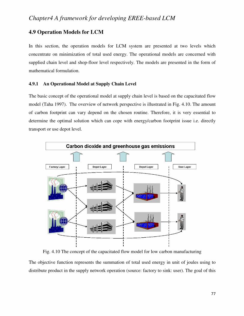
Chapter4 A framework for developing EREE-based LCM
77
4.9 Operation Models for LCM
In this section, the operation models for LCM system are presented at two levels which
concentrate on minimization of total used energy. The operational models are concerned with
supplied chain level and shop-floor level respectively. The models are presented in the form of
mathematical formulation.
4.9.1 An Operational Model at Supply Chain Level
The basic concept of the operational model at supply chain level is based on the capacitated flow
model (Taha 1997). The overview of network perspective is illustrated in Fig. 4.10. The amount
of carbon footprint can vary depend on the chosen routine. Therefore, it is very essential to
determine the optimal solution which can cope with energy/carbon footprint issue i.e. directly
transport or use depot level.
Fig. 4.10 The concept of the capacitated flow model for low carbon manufacturing
The objective function represents the summation of total used energy in unit of joules using to
distribute product in the supply network operation (source: factory to sink: user). The goal of this
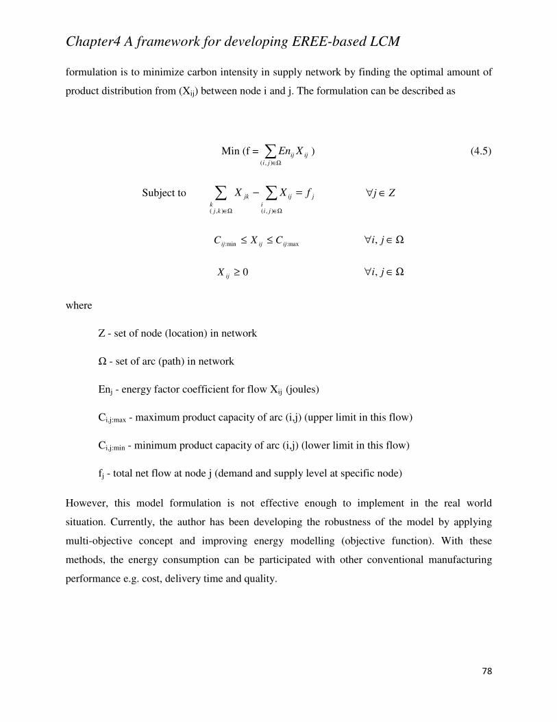
Chapter4 A framework for developing EREE-based LCM
78
formulation is to minimize carbon intensity in supply network by finding the optimal amount of
product distribution from (Xij) between node i and j. The formulation can be described as
Min (f = ∑Ω∈),( ji
ijij XEn ) (4.5)
Subject to ∑ ∑Ω∈ Ω∈
=−
),( ),(kjk
jii
jijjk fXX Zj ∈∀
:max:min ijijij CXC ≤≤ Ω∈∀ ji,
0≥ijX Ω∈∀ ji,
where
Z - set of node (location) in network
Ω - set of arc (path) in network
Enj - energy factor coefficient for flow Xij (joules)
Ci,j:max - maximum product capacity of arc (i,j) (upper limit in this flow)
Ci,j:min - minimum product capacity of arc (i,j) (lower limit in this flow)
fj - total net flow at node j (demand and supply level at specific node)
However, this model formulation is not effective enough to implement in the real world
situation. Currently, the author has been developing the robustness of the model by applying
multi-objective concept and improving energy modelling (objective function). With these
methods, the energy consumption can be participated with other conventional manufacturing
performance e.g. cost, delivery time and quality.
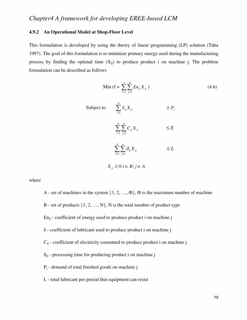
Chapter4 A framework for developing EREE-based LCM
79
4.9.2 An Operational Model at Shop-Floor Level
This formulation is developed by using the theory of linear programming (LP) solution (Taha
1997). The goal of this formulation is to minimize primary energy used during the manufacturing
process by finding the optimal time (Xij) to produce product i on machine j. The problem
formulation can be described as follows
Min (f = ∑∑= =
n
i j
ijij XEn1 1
φ
) (4.6)
Subject to ∑=
N
i
ijij XS1
jP≥
∑∑= =
N
i j
ijij XC1 1
φ
E≤
∑∑= =
N
i j
ijij X1 1
φ
δ L≤
AjBiX ij ∈∈≥ ;;0
where
A - set of machines in the system 1, 2, …, Ф, Ф is the maximum number of machine
B - set of products 1, 2, …, N, N is the total number of product type
Enij - coefficient of energy used to produce product i on machine j
δ - coefficient of lubricant used to produce product i on machine j
Cij - coefficient of electricity consumed to produce product i on machine j
Sij - processing time for producing product i on machine j
Pj - demand of total finished goods on machine j
L - total lubricant per period that equipment can resist
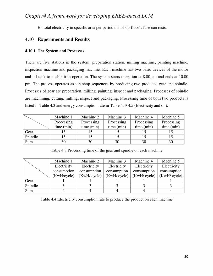
Chapter4 A framework for developing EREE-based LCM
80
E - total electricity in specific area per period that shop-floor’s fuse can resist
4.10 Experiments and Results
4.10.1 The System and Processes
There are five stations in the system: preparation station, milling machine, painting machine,
inspection machine and packaging machine. Each machine has two basic devices of the motor
and oil tank to enable it in operation. The system starts operation at 8.00 am and ends at 10.00
pm. The process operates as job shop sequences by producing two products: gear and spindle.
Processes of gear are preparation, milling, painting, inspect and packaging. Processes of spindle
are machining, cutting, milling, inspect and packaging. Processing time of both two products is
listed in Table 4.3 and energy consumption rate in Table 4.4/ 4.5 (Electricity and oil).
Machine 1 Machine 2 Machine 3 Machine 4 Machine 5 Processing time (min)
Processing time (min)
Processing time (min)
Processing time (min)
Processing time (min)
Gear 15 15 15 15 15
Spindle 15 15 15 15 15 Sum 30 30 30 30 30
Table 4.3 Processing time of the gear and spindle on each machine
Machine 1 Machine 2 Machine 3 Machine 4 Machine 5 Electricity
consumption (KwH/cycle)
Electricity consumption (KwH/ cycle)
Electricity consumption (KwH/ cycle)
Electricity consumption (KwH/ cycle)
Electricity consumption (KwH/ cycle)
Gear 1 1 1 1 1
Spindle 3 3 3 3 3 Sum 4 4 4 4 4
Table 4.4 Electricity consumption rate to produce the product on each machine
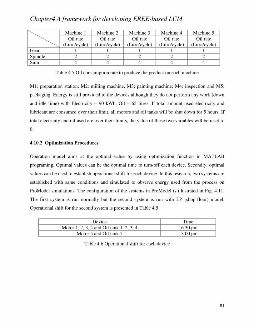
Chapter4 A framework for developing EREE-based LCM
81
Machine 1 Machine 2 Machine 3 Machine 4 Machine 5 Oil rate
(Litre/cycle) Oil rate
(Litre/cycle) Oil rate
(Litre/cycle) Oil rate
(Litre/cycle) Oil rate
(Litre/cycle)
Gear 1 1 1 1 1
Spindle 2 2 2 2 2
Sum 4 4 4 4 4
Table 4.5 Oil consumption rate to produce the product on each machine
M1: preparation station; M2: milling machine, M3; painting machine; M4: inspection and M5:
packaging. Energy is still provided to the devices although they do not perform any work (down
and idle time) with Electricity = 90 kWh, Oil = 65 litres. If total amount used electricity and
lubricant are consumed over their limit, all motors and oil tanks will be shut down for 5 hours. If
total electricity and oil used are over their limits, the value of these two variables will be reset to
0.
4.10.2 Optimization Procedures
Operation model aims at the optimal value by using optimization function in MATLAB
programing. Optimal values can be the optimal time to turn-off each device. Secondly, optimal
values can be used to establish operational shift for each device. In this research, two systems are
established with same conditions and simulated to observe energy used from the process on
ProModel simulations. The configuration of the systems in ProModel is illustrated in Fig. 4.11.
The first system is run normally but the second system is run with LP (shop-floor) model.
Operational shift for the second system is presented in Table 4.5.
Device Time Motor 1, 2, 3, 4 and Oil tank 1, 2, 3, 4 16.30 pm
Motor 5 and Oil tank 5 13.00 pm
Table 4.6 Operational shift for each device
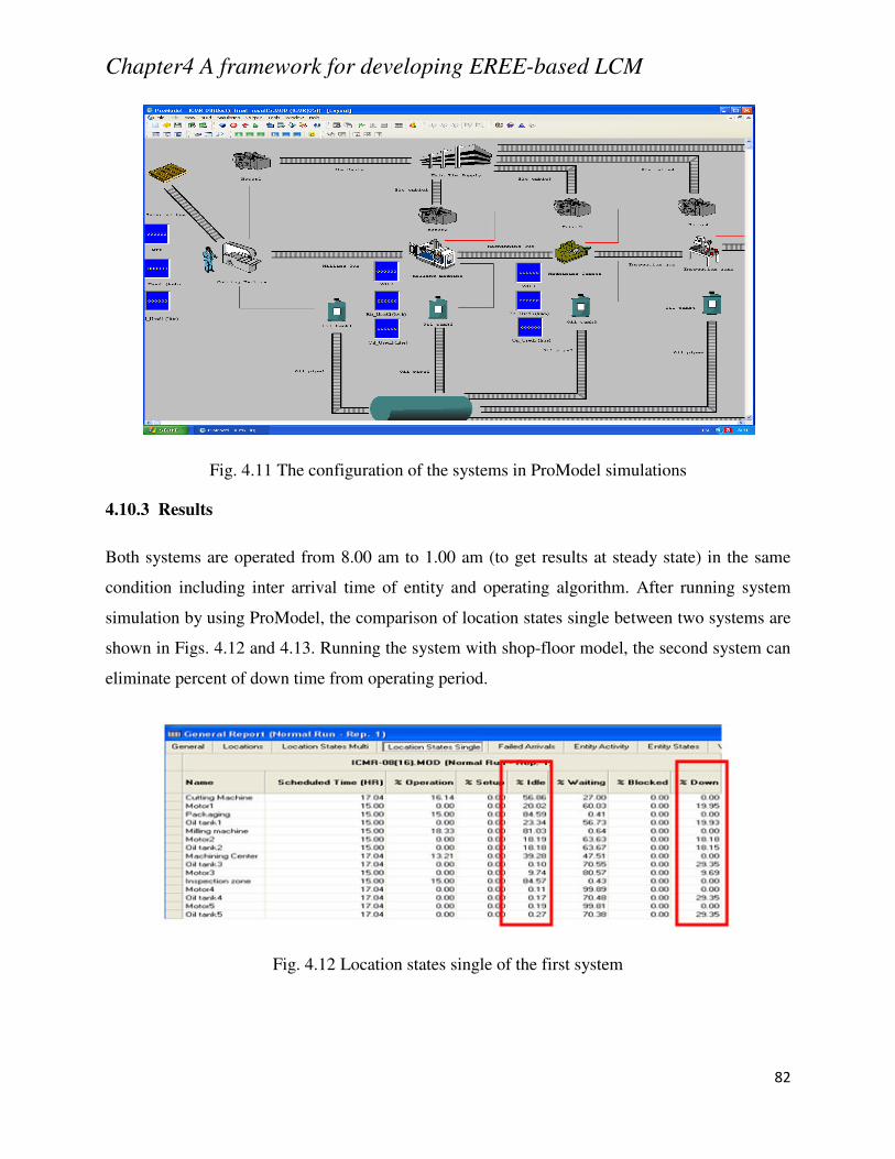
Chapter4 A framework for developing EREE-based LCM
82
Fig. 4.11 The configuration of the systems in ProModel simulations
4.10.3 Results
Both systems are operated from 8.00 am to 1.00 am (to get results at steady state) in the same
condition including inter arrival time of entity and operating algorithm. After running system
simulation by using ProModel, the comparison of location states single between two systems are
shown in Figs. 4.12 and 4.13. Running the system with shop-floor model, the second system can
eliminate percent of down time from operating period.
Fig. 4.12 Location states single of the first system
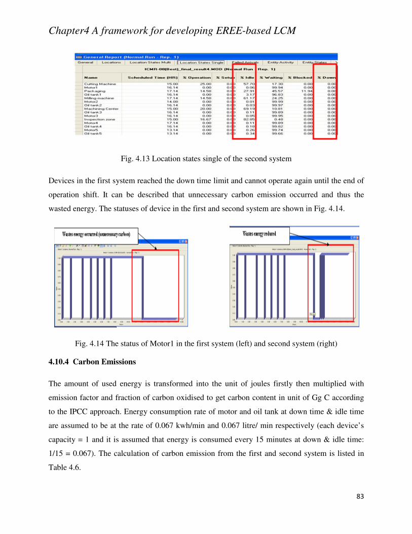
Chapter4 A framework for developing EREE-based LCM
83
Fig. 4.13 Location states single of the second system
Devices in the first system reached the down time limit and cannot operate again until the end of
operation shift. It can be described that unnecessary carbon emission occurred and thus the
wasted energy. The statuses of device in the first and second system are shown in Fig. 4.14.
Fig. 4.14 The status of Motor1 in the first system (left) and second system (right)
4.10.4 Carbon Emissions
The amount of used energy is transformed into the unit of joules firstly then multiplied with
emission factor and fraction of carbon oxidised to get carbon content in unit of Gg C according
to the IPCC approach. Energy consumption rate of motor and oil tank at down time & idle time
are assumed to be at the rate of 0.067 kwh/min and 0.067 litre/ min respectively (each device’s
capacity = 1 and it is assumed that energy is consumed every 15 minutes at down & idle time:
1/15 = 0.067). The calculation of carbon emission from the first and second system is listed in
Table 4.6.
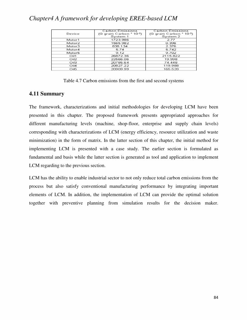
Chapter4 A framework for developing EREE-based LCM
84
Table 4.7 Carbon emissions from the first and second systems
4.11 Summary
The framework, characterizations and initial methodologies for developing LCM have been
presented in this chapter. The proposed framework presents appropriated approaches for
different manufacturing levels (machine, shop-floor, enterprise and supply chain levels)
corresponding with characterizations of LCM (energy efficiency, resource utilization and waste
minimization) in the form of matrix. In the latter section of this chapter, the initial method for
implementing LCM is presented with a case study. The earlier section is formulated as
fundamental and basis while the latter section is generated as tool and application to implement
LCM regarding to the previous section.
LCM has the ability to enable industrial sector to not only reduce total carbon emissions from the
process but also satisfy conventional manufacturing performance by integrating important
elements of LCM. In addition, the implementation of LCM can provide the optimal solution
together with preventive planning from simulation results for the decision maker.
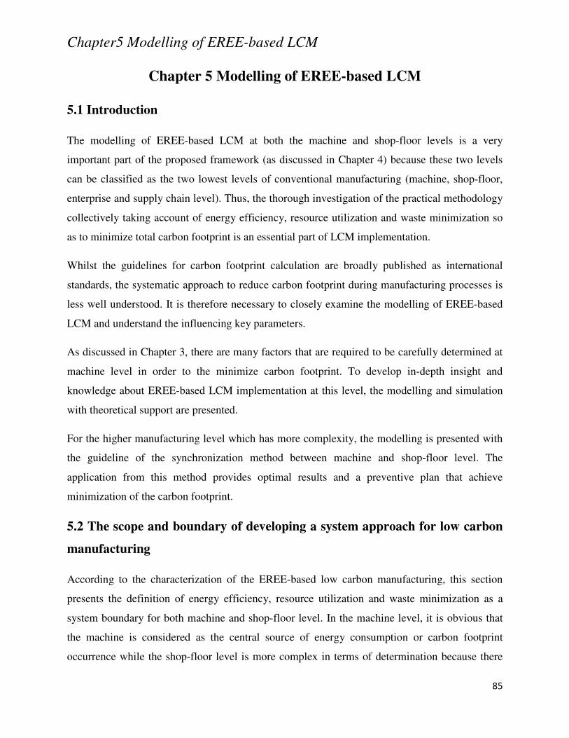
Chapter5 Modelling of EREE-based LCM
85
Chapter 5 Modelling of EREE-based LCM
5.1 Introduction
The modelling of EREE-based LCM at both the machine and shop-floor levels is a very
important part of the proposed framework (as discussed in Chapter 4) because these two levels
can be classified as the two lowest levels of conventional manufacturing (machine, shop-floor,
enterprise and supply chain level). Thus, the thorough investigation of the practical methodology
collectively taking account of energy efficiency, resource utilization and waste minimization so
as to minimize total carbon footprint is an essential part of LCM implementation.
Whilst the guidelines for carbon footprint calculation are broadly published as international
standards, the systematic approach to reduce carbon footprint during manufacturing processes is
less well understood. It is therefore necessary to closely examine the modelling of EREE-based
LCM and understand the influencing key parameters.
As discussed in Chapter 3, there are many factors that are required to be carefully determined at
machine level in order to the minimize carbon footprint. To develop in-depth insight and
knowledge about EREE-based LCM implementation at this level, the modelling and simulation
with theoretical support are presented.
For the higher manufacturing level which has more complexity, the modelling is presented with
the guideline of the synchronization method between machine and shop-floor level. The
application from this method provides optimal results and a preventive plan that achieve
minimization of the carbon footprint.
5.2 The scope and boundary of developing a system approach for low carbon
manufacturing
According to the characterization of the EREE-based low carbon manufacturing, this section
presents the definition of energy efficiency, resource utilization and waste minimization as a
system boundary for both machine and shop-floor level. In the machine level, it is obvious that
the machine is considered as the central source of energy consumption or carbon footprint
occurrence while the shop-floor level is more complex in terms of determination because there
Chapter5 Modelling of EREE-based LCM
86
are many available machines in the system. Some machines might not be selected to perform a
work assignment. Therefore, the boundary for the machine level focuses at the machine
operations and its environment while the shop-floor level focuses on the management of FMS
system and the operational sequence with total energy consumption. The definitions of
characterization in the machine level are expressed as follow;
(1) Energy efficiency: Normally, the definition of energy efficiency is referred to the
objective which aims to reduce the amount of energy consumption used to provide
products and services. Most development methods for energy efficiency are provided by
achieving efficient technology or production process (Diesendorf 2007). With this
information, it can be implied that the term of energy efficiency at the machine level is
the machining operations including machine set-up and cutting process which consumes
lower energy consumption while the same service can also be served. On the other hand,
it can be referred to the machining operation with the minimization of energy
consumption while the other objectives (maximization of profit and minimization of total
production time) are also satisfied. Thus, this research aims to investigate and develop the
approach and application which can be implemented to the machine level by providing
the optimal machine set-up concerned with a multi objective concept. For energy
efficiency at the shop-floor level, the problem of process sequence and work assignment
are required to integrate with the evaluation of the impact from energy consumption. This
concept means even the traditional FMS problems can be solved with optimal solution
and the minimization of energy consumption must also be satisfied. Hence, this research
also aims to investigate and develop the methods and tools for energy efficiency at the
shop-floor level by integrating the application for the machine level as a sub sequence
with the optimization method.
(2) Resource utilization: Normally, the term of resource can be referred to tangible and
intangible resources which have limited availability can be scheduled/ assigned work and
even utilized by users (Wysocki 2009). The type of resource can be categorized as a
natural resource (non-renewable resource and renewable resource etc.), human resource
(talents, skills and abilities etc.) and tangible resource (equipment, machines and vehicles
etc.) while resource utilization in manufacturing systems mean the percentage that a
Chapter5 Modelling of EREE-based LCM
87
resource is used in the considered time period (Harrell 2003). The equation for resource
utilization is expressed in Equation 5.1. Thus, this research focuses on the utilization of
resources in the manufacturing process which can affect the level of energy consumption
and carbon footprint such as production hours of machines, selection of cutting tools and
material systems. The utilization of resources which is not related to the emission factor
will not be considered.
% ! "#! ! $!%&'$(! "% '%!)&*+ (&,%")!$!) -!$"&) &. "#! (5.1)
(3) Waste minimization: According to the philosophy of just in time (JIT), waste from
manufacturing is not only referred to as the scrap or garbage from the process but it can
also represent any resource that adds cost but does not add value to the product
(Tompkins 2003). Waste in JIT, thus, can be categorized into seven types as waste from
overproduction, time on hand (waiting), transporting, processing itself, unnecessary stock
on hand, unnecessary motion and producing defective goods (LU 1985). Hence, waste
within EREE-based LCM system boundary refers to any resource that causes
unnecessary energy consumption and carbon footprint (all considered wastes are related
to the emission factor). For example, wastes that are focused in this research are
maintenance downtime, machine down time and operator error (motion that causes
unnecessary energy consumption). The preventive plan which has an objective to
minimize waste in EREE-based LCM for FMS is a focus in this research.
Fig. 5.1 presents the cause of carbon footprint in FMS from energy consumption,
utilization of resource and waste. The main energy consumption comes from the
production process while the selection of resource (machine, cutting tool and material
handling systems) and unnecessary waste (down time, idle time and error motion) related
to emission factors are also determined for the total carbon footprint.
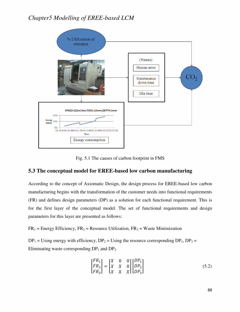
Chapter5 Modelling of EREE-based LCM
88
Fig. 5.1 The causes of carbon footprint in FMS
5.3 The conceptual model for EREE-based low carbon manufacturing
According to the concept of Axiomatic Design, the design process for EREE-based low carbon
manufacturing begins with the transformation of the customer needs into functional requirements
(FR) and defines design parameters (DP) as a solution for each functional requirement. This is
for the first layer of the conceptual model. The set of functional requirements and design
parameters for this layer are presented as follows:
FR1 = Energy Efficiency, FR2 = Resource Utilization, FR3 = Waste Minimization
DP1 = Using energy with efficiency, DP2 = Using the resource corresponding DP1, DP3 =
Eliminating waste corresponding DP1 and DP2
/ 0 /1 0 01 1 01 1 10 /0 (5.2)
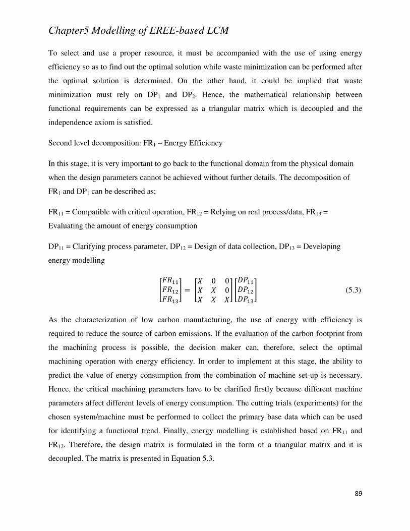
Chapter5 Modelling of EREE-based LCM
89
To select and use a proper resource, it must be accompanied with the use of using energy
efficiency so as to find out the optimal solution while waste minimization can be performed after
the optimal solution is determined. On the other hand, it could be implied that waste
minimization must rely on DP1 and DP2. Hence, the mathematical relationship between
functional requirements can be expressed as a triangular matrix which is decoupled and the
independence axiom is satisfied.
Second level decomposition: FR1 – Energy Efficiency
In this stage, it is very important to go back to the functional domain from the physical domain
when the design parameters cannot be achieved without further details. The decomposition of
FR1 and DP1 can be described as;
FR11 = Compatible with critical operation, FR12 = Relying on real process/data, FR13 =
Evaluating the amount of energy consumption
DP11 = Clarifying process parameter, DP12 = Design of data collection, DP13 = Developing
energy modelling
/ 0 /1 0 01 1 01 1 10 /
0 (5.3)
As the characterization of low carbon manufacturing, the use of energy with efficiency is
required to reduce the source of carbon emissions. If the evaluation of the carbon footprint from
the machining process is possible, the decision maker can, therefore, select the optimal
machining operation with energy efficiency. In order to implement at this stage, the ability to
predict the value of energy consumption from the combination of machine set-up is necessary.
Hence, the critical machining parameters have to be clarified firstly because different machine
parameters affect different levels of energy consumption. The cutting trials (experiments) for the
chosen system/machine must be performed to collect the primary base data which can be used
for identifying a functional trend. Finally, energy modelling is established based on FR11 and
FR12. Therefore, the design matrix is formulated in the form of a triangular matrix and it is
decoupled. The matrix is presented in Equation 5.3.
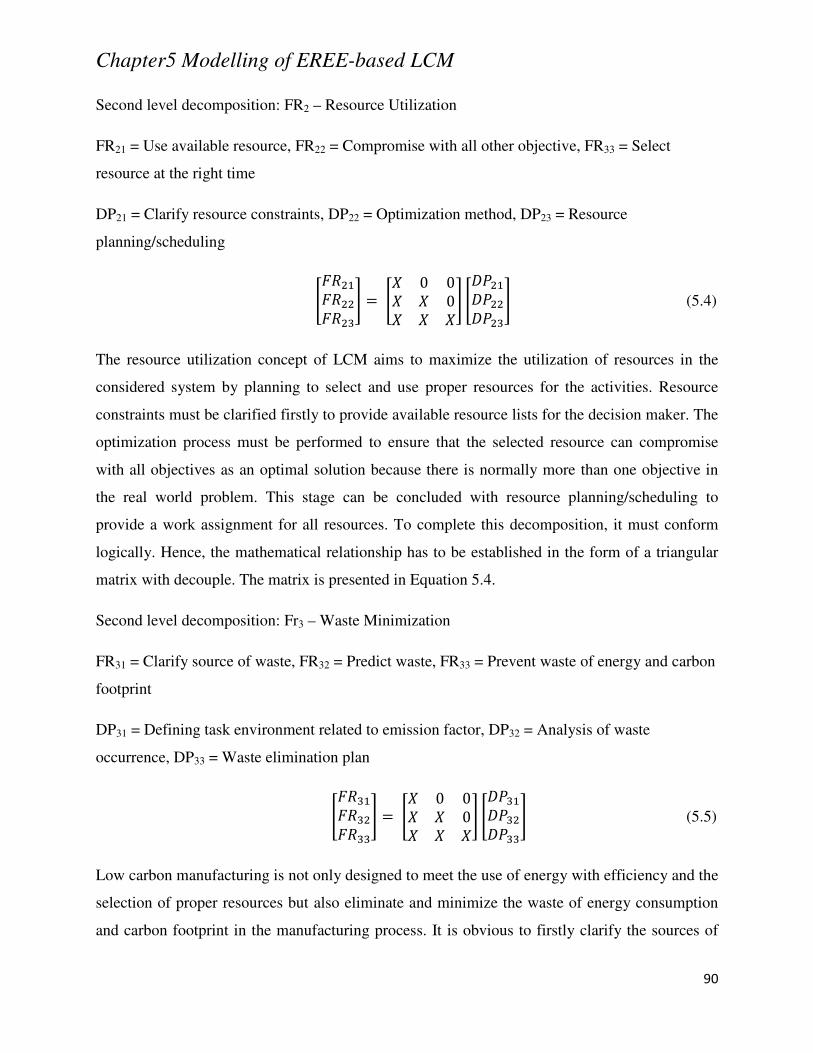
Chapter5 Modelling of EREE-based LCM
90
Second level decomposition: FR2 – Resource Utilization
FR21 = Use available resource, FR22 = Compromise with all other objective, FR33 = Select
resource at the right time
DP21 = Clarify resource constraints, DP22 = Optimization method, DP23 = Resource
planning/scheduling
/ 0 /1 0 01 1 01 1 10 /
0 (5.4)
The resource utilization concept of LCM aims to maximize the utilization of resources in the
considered system by planning to select and use proper resources for the activities. Resource
constraints must be clarified firstly to provide available resource lists for the decision maker. The
optimization process must be performed to ensure that the selected resource can compromise
with all objectives as an optimal solution because there is normally more than one objective in
the real world problem. This stage can be concluded with resource planning/scheduling to
provide a work assignment for all resources. To complete this decomposition, it must conform
logically. Hence, the mathematical relationship has to be established in the form of a triangular
matrix with decouple. The matrix is presented in Equation 5.4.
Second level decomposition: Fr3 – Waste Minimization
FR31 = Clarify source of waste, FR32 = Predict waste, FR33 = Prevent waste of energy and carbon
footprint
DP31 = Defining task environment related to emission factor, DP32 = Analysis of waste
occurrence, DP33 = Waste elimination plan
/ 0 /1 0 01 1 01 1 10 /
0 (5.5)
Low carbon manufacturing is not only designed to meet the use of energy with efficiency and the
selection of proper resources but also eliminate and minimize the waste of energy consumption
and carbon footprint in the manufacturing process. It is obvious to firstly clarify the sources of
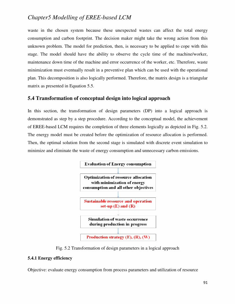
Chapter5 Modelling of EREE-based LCM
91
waste in the chosen system because these unexpected wastes can affect the total energy
consumption and carbon footprint. The decision maker might take the wrong action from this
unknown problem. The model for prediction, then, is necessary to be applied to cope with this
stage. The model should have the ability to observe the cycle time of the machine/worker,
maintenance down time of the machine and error occurrence of the worker, etc. Therefore, waste
minimization must eventually result in a preventive plan which can be used with the operational
plan. This decomposition is also logically performed. Therefore, the matrix design is a triangular
matrix as presented in Equation 5.5.
5.4 Transformation of conceptual design into logical approach
In this section, the transformation of design parameters (DP) into a logical approach is
demonstrated as step by a step procedure. According to the conceptual model, the achievement
of EREE-based LCM requires the completion of three elements logically as depicted in Fig. 5.2.
The energy model must be created before the optimization of resource allocation is performed.
Then, the optimal solution from the second stage is simulated with discrete event simulation to
minimize and eliminate the waste of energy consumption and unnecessary carbon emissions.
Fig. 5.2 Transformation of design parameters in a logical approach
5.4.1 Energy efficiency
Objective: evaluate energy consumption from process parameters and utilization of resource
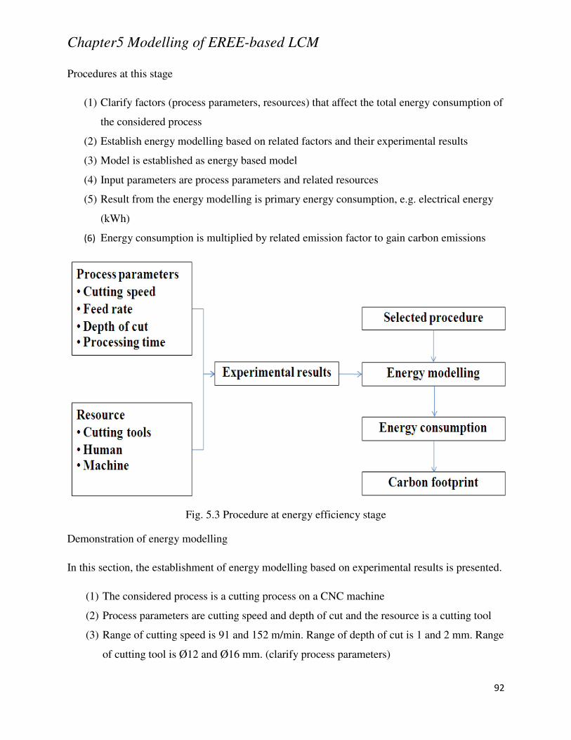
Chapter5 Modelling of EREE-based LCM
92
Procedures at this stage
(1) Clarify factors (process parameters, resources) that affect the total energy consumption of
the considered process
(2) Establish energy modelling based on related factors and their experimental results
(3) Model is established as energy based model
(4) Input parameters are process parameters and related resources
(5) Result from the energy modelling is primary energy consumption, e.g. electrical energy
(kWh)
(6) Energy consumption is multiplied by related emission factor to gain carbon emissions
Fig. 5.3 Procedure at energy efficiency stage
Demonstration of energy modelling
In this section, the establishment of energy modelling based on experimental results is presented.
(1) The considered process is a cutting process on a CNC machine
(2) Process parameters are cutting speed and depth of cut and the resource is a cutting tool
(3) Range of cutting speed is 91 and 152 m/min. Range of depth of cut is 1 and 2 mm. Range
of cutting tool is Ø12 and Ø16 mm. (clarify process parameters)
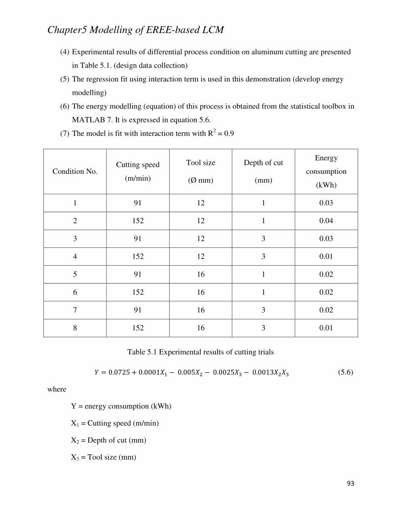
Chapter5 Modelling of EREE-based LCM
93
(4) Experimental results of differential process condition on aluminum cutting are presented
in Table 5.1. (design data collection)
(5) The regression fit using interaction term is used in this demonstration (develop energy
modelling)
(6) The energy modelling (equation) of this process is obtained from the statistical toolbox in
MATLAB 7. It is expressed in equation 5.6.
(7) The model is fit with interaction term with R2 = 0.9
Condition No. Cutting speed
(m/min)
Tool size
(Ø mm)
Depth of cut
(mm)
Energy
consumption
(kWh)
1 91 12 1 0.03
2 152 12 1 0.04
3 91 12 3 0.03
4 152 12 3 0.01
5 91 16 1 0.02
6 152 16 1 0.02
7 91 16 3 0.02
8 152 16 3 0.01
Table 5.1 Experimental results of cutting trials
2 0.0725 7 0.00011 9 0.0051 9 0.00251 9 0.001311 (5.6)
where
Y = energy consumption (kWh)
X1 = Cutting speed (m/min)
X2 = Depth of cut (mm)
X3 = Tool size (mm)
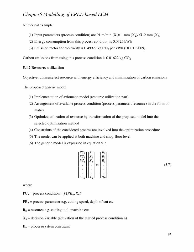
Chapter5 Modelling of EREE-based LCM
94
Numerical example
(1) Input parameters (process condition) are 91 m/min (X1)/ 1 mm (X2)/ Ø12 mm (X3)
(2) Energy consumption from this process condition is 0.0325 kWh
(3) Emission factor for electricity is 0.49927 kg CO2 per kWh (DECC 2009)
Carbon emissions from using this process condition is 0.01622 kg CO2
5.4.2 Resource utilization
Objective: utilize/select resource with energy efficiency and minimization of carbon emissions
The proposed generic model
(1) Implementation of axiomatic model (resource utilization part)
(2) Arrangement of available process condition (process parameter, resource) in the form of
matrix
(3) Optimize utilization of resource by transformation of the proposed model into the
selected optimization method
(4) Constraints of the considered process are involved into the optimization procedure
(5) The model can be applied at both machine and shop-floor level
(6) The generic model is expressed in equation 5.7
;<<<<<=>>>...>?@A
AAAAB ;<<<<<=111...1,@A
AAAAB C
;<<<<<=DDD...D?@A
AAAAB (5.7)
where
PCn = process condition = ,, , PRn = process parameter e.g. cutting speed, depth of cut etc.
Rn = resource e.g. cutting tool, machine etc.
Xn = decision variable (activation of the related process condition n)
Bn = process/system constraint

Chapter5 Modelling of EREE-based LCM
95
Perspective of the generic model
(1) Process/system constraints define the size of decision matrix in both machine and shop-
floor level.
(2) The left hand side matrix is the available process condition
(3) The second matrix is the decision variable matrix
(4) The third matrix is the constraint matrix
(5) Objective function of energy consumption can be established based on the evaluation
model at the first stage.
(6) For example: Ob = 0.01X1 + 0.02X2 + 0.003X3
(7) The constant values are obtained from the evaluation model presented in the first stage.
(8) For instance, the value of 0.01(kWh) is defined when 152 m/min, Ø12mm, 1mm are used
as process condition.
(9) If process condition 1 and 2 (X1, X2) are activated (selected), the total energy
consumption is 0.03 kWh.
(10) The arrangement of the decision matrix is dependent on the selected optimization model.
(11) The explanation of resource utilization is expressed in Fig. 5.4.
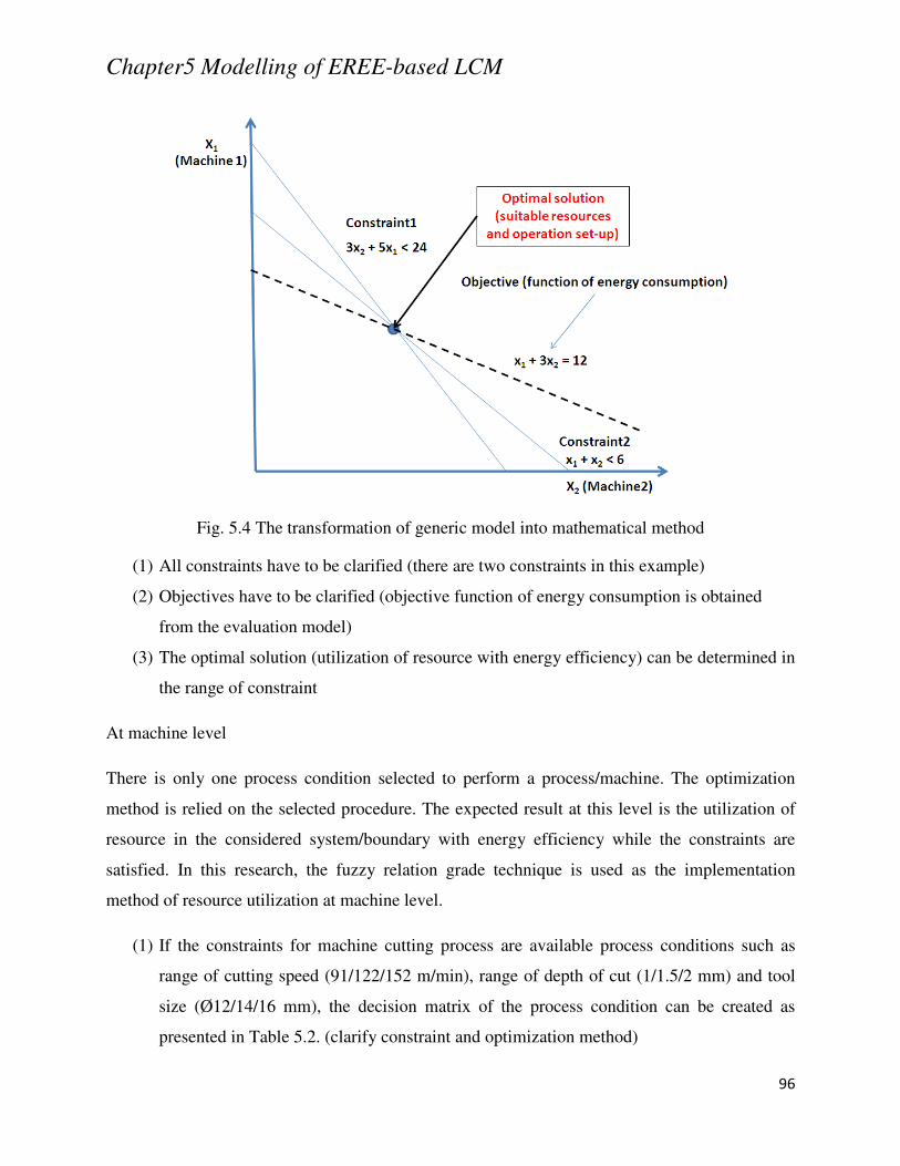
Chapter5 Modelling of EREE-based LCM
96
Fig. 5.4 The transformation of generic model into mathematical method
(1) All constraints have to be clarified (there are two constraints in this example)
(2) Objectives have to be clarified (objective function of energy consumption is obtained
from the evaluation model)
(3) The optimal solution (utilization of resource with energy efficiency) can be determined in
the range of constraint
At machine level
There is only one process condition selected to perform a process/machine. The optimization
method is relied on the selected procedure. The expected result at this level is the utilization of
resource in the considered system/boundary with energy efficiency while the constraints are
satisfied. In this research, the fuzzy relation grade technique is used as the implementation
method of resource utilization at machine level.
(1) If the constraints for machine cutting process are available process conditions such as
range of cutting speed (91/122/152 m/min), range of depth of cut (1/1.5/2 mm) and tool
size (Ø12/14/16 mm), the decision matrix of the process condition can be created as
presented in Table 5.2. (clarify constraint and optimization method)
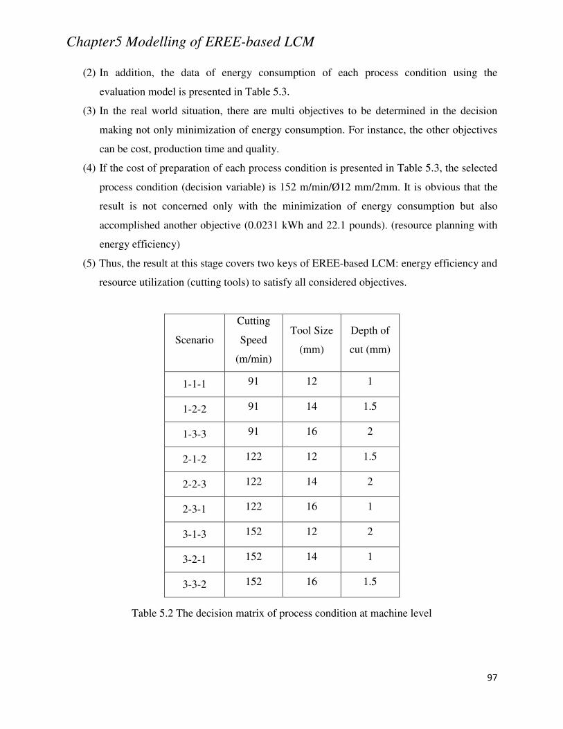
Chapter5 Modelling of EREE-based LCM
97
(2) In addition, the data of energy consumption of each process condition using the
evaluation model is presented in Table 5.3.
(3) In the real world situation, there are multi objectives to be determined in the decision
making not only minimization of energy consumption. For instance, the other objectives
can be cost, production time and quality.
(4) If the cost of preparation of each process condition is presented in Table 5.3, the selected
process condition (decision variable) is 152 m/min/Ø12 mm/2mm. It is obvious that the
result is not concerned only with the minimization of energy consumption but also
accomplished another objective (0.0231 kWh and 22.1 pounds). (resource planning with
energy efficiency)
(5) Thus, the result at this stage covers two keys of EREE-based LCM: energy efficiency and
resource utilization (cutting tools) to satisfy all considered objectives.
Scenario
Cutting
Speed
(m/min)
Tool Size
(mm)
Depth of
cut (mm)
1-1-1 91 12 1
1-2-2 91 14 1.5
1-3-3 91 16 2
2-1-2 122 12 1.5
2-2-3 122 14 2
2-3-1 122 16 1
3-1-3 152 12 2
3-2-1 152 14 1
3-3-2 152 16 1.5
Table 5.2 The decision matrix of process condition at machine level
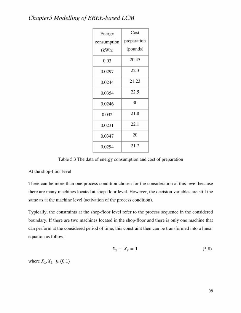
Chapter5 Modelling of EREE-based LCM
98
Energy
consumption
(kWh)
Cost
preparation
(pounds)
0.03 20.45
0.0297 22.3
0.0244 21.23
0.0354 22.5
0.0246 30
0.032 21.8
0.0231 22.1
0.0347 20
0.0294 21.7
Table 5.3 The data of energy consumption and cost of preparation
At the shop-floor level
There can be more than one process condition chosen for the consideration at this level because
there are many machines located at shop-floor level. However, the decision variables are still the
same as at the machine level (activation of the process condition).
Typically, the constraints at the shop-floor level refer to the process sequence in the considered
boundary. If there are two machines located in the shop-floor and there is only one machine that
can perform at the considered period of time, this constraint then can be transformed into a linear
equation as follow;
1 7 1 1 (5.8)
where 1, 1 F G0,1H
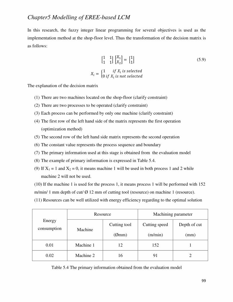
Chapter5 Modelling of EREE-based LCM
99
In this research, the fuzzy integer linear programming for several objectives is used as the
implementation method at the shop-floor level. Thus the transformation of the decision matrix is
as follows:
I1 11 1J 11 I11J (5.9)
1" K1 1" L LMMNMO0 1" L LMMNMOP The explanation of the decision matrix
(1) There are two machines located on the shop-floor (clarify constraint)
(2) There are two processes to be operated (clarify constraint)
(3) Each process can be performed by only one machine (clarify constraint)
(4) The first row of the left hand side of the matrix represents the first operation
(optimization method)
(5) The second row of the left hand side matrix represents the second operation
(6) The constant value represents the process sequence and boundary
(7) The primary information used at this stage is obtained from the evaluation model
(8) The example of primary information is expressed in Table 5.4.
(9) If X1 = 1 and X2 = 0, it means machine 1 will be used in both process 1 and 2 while
machine 2 will not be used.
(10) If the machine 1 is used for the process 1, it means process 1 will be performed with 152
m/min/ 1 mm depth of cut/ Ø 12 mm of cutting tool (resource) on machine 1 (resource).
(11) Resources can be well utilized with energy efficiency regarding to the optimal solution
Energy
consumption
Resource Machining parameter
Machine Cutting tool
(Ømm)
Cutting speed
(m/min)
Depth of cut
(mm)
0.01 Machine 1 12 152 1
0.02 Machine 2 16 91 2
Table 5.4 The primary information obtained from the evaluation model
Chapter5 Modelling of EREE-based LCM
100
5.4.3 Waste minimization
Objective: minimize and eliminate waste of energy consumption and carbon emissions
Procedure of converting waste into energy consumption and carbon emission
(1) Clarify waste that can be a source of carbon emissions
(2) Waste are converted into waste of energy consumption and multiplied by related
emission factor to gain carbon emissions
(3) Waste concerned in this research is energy and time based
(4) Transformation of waste into carbon emissions are presented in Equation 5.10
(5) Waste can be maintenance down time, idle time and human error etc.
WT1 (min) * CW1 (Unit of used energy/ min) * EW1 = CO2W1 (5.10)
WT2 (min) * CW2 (Unit of used energy/ min) * EW2 = CO2W2
.
WTn (min) * CWn (Unit of used energy/ min) * EWn = CO2Wn
.
WTN (min) * CWN (Unit of used energy/ min) * EWN = CO2WN
TCO2 = CO2W1 + CO2W2 + … + CO2Wn + … + CO2WN
where
WTn = Total time of waste type n occurred (min)
CWn = Consumed energy related to waste n (unit of used energy/ min)
EWn = Emission factor of waste type n
TCO2 = Total carbon emission from wastes at the considered system
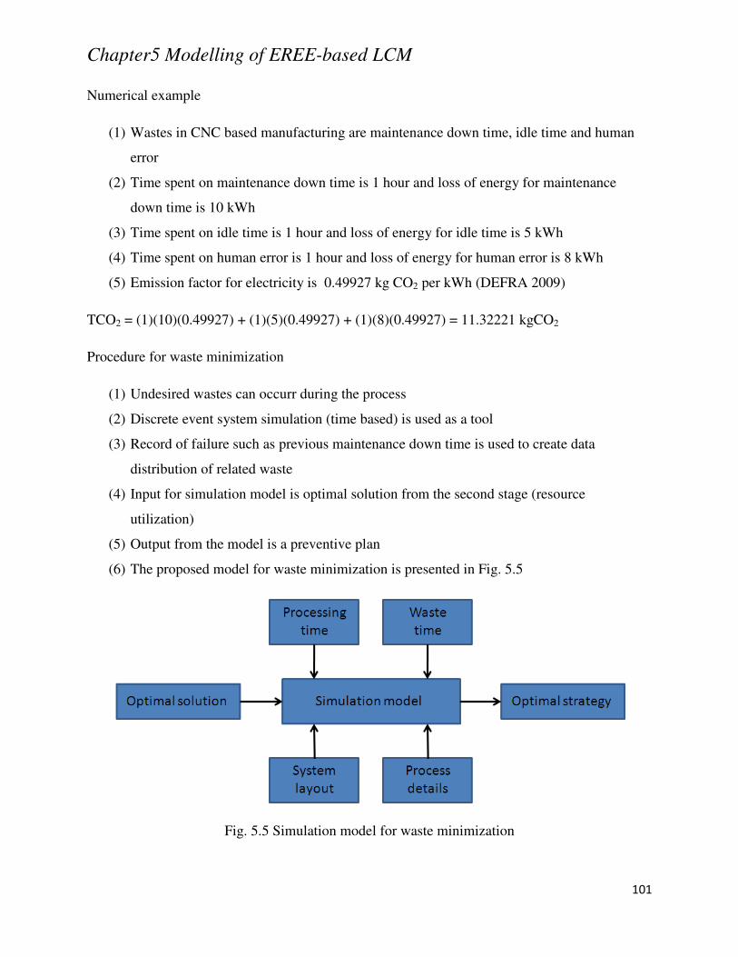
Chapter5 Modelling of EREE-based LCM
101
Numerical example
(1) Wastes in CNC based manufacturing are maintenance down time, idle time and human
error
(2) Time spent on maintenance down time is 1 hour and loss of energy for maintenance
down time is 10 kWh
(3) Time spent on idle time is 1 hour and loss of energy for idle time is 5 kWh
(4) Time spent on human error is 1 hour and loss of energy for human error is 8 kWh
(5) Emission factor for electricity is 0.49927 kg CO2 per kWh (DEFRA 2009)
TCO2 = (1)(10)(0.49927) + (1)(5)(0.49927) + (1)(8)(0.49927) = 11.32221 kgCO2
Procedure for waste minimization
(1) Undesired wastes can occurr during the process
(2) Discrete event system simulation (time based) is used as a tool
(3) Record of failure such as previous maintenance down time is used to create data
distribution of related waste
(4) Input for simulation model is optimal solution from the second stage (resource
utilization)
(5) Output from the model is a preventive plan
(6) The proposed model for waste minimization is presented in Fig. 5.5
Fig. 5.5 Simulation model for waste minimization

Chapter5 Modelling of EREE-based LCM
102
Numerical example
(1) The input of the simulation model (process condition) is machine type A, cutting tool
Ø12 mm, cutting speed 122m/min and depth of cut 1mm performed on aluminum cutting
(2) Simulation results are presented in Table 5.5
(3) Primary energy consumption is electricity
(4) Emission factor for electricity is 0.49927kgCO2perkWh
(5) Loss of energy from idle time is 5kWh/hour
(6) Loss of energy from maintenance down time is 10 kWh/hour
(7) Carbon emission from waste = (3.83)(0.0435)(5)(0.49927) + (3.83)(0.5217)(10)(0.49927)
= 10.4 kgCO2
(8) If the carbon emission from performing this process condition is 0.016 kgCO2 (obtained
from the evaluation model), the total carbon emission is 10.4 + 0.016 = 10.42 kgCO2
(9) To prevent unnecessary carbon emissions from waste, the preventive plan must be
established
(10) The demonstration of the preventive plan will be discussed in machine and shop-floor
modelling
Name
Scheduled
Time (HR) % Operation
%
Setup
%
Idle
%
Waiting
%
Blocked
%
Down
Loc1 3.83 43.48 0 4.35 0 0 52.17
Table 5.5 Simulation of waste during the process using discrete event simulation
Chapter5 Modelling of EREE-based LCM
103
5.5 The systematic approach for applying the conceptual model to achieve
sustainable manufacturing
This section presents the method of using the conceptual model for both machine and shop-floor
levels as a systematic approach. It could be, on the other hand, implied that this model must be
firstly applied to the lowest level of manufacturing structure (machine level) and then go through
the next higher level in order to the minimize energy consumption and carbon footprint in every
point of the system. In Fig. 5.6, the overall perspective of the systematic approach is presented.
There are six steps for using the integrated model at machine and shop-floor level.
(1) Machining operations analysis: First of all at machine level, it is very important to
understand operations/process of the considered machine in order to seek out what factors
can affect the amount of energy consumption and carbon footprint. Some factors might
make a different effect on the total energy consumption compared to the other factors. So,
it is very useful in the preparation of preparing these details to use energy efficiency.
Resources (such as a cutting tool) which are used in the operations are also concerned to
increase the utilization of resource. The details of waste related to the total carbon
footprint are also required to analyze how the waste of energy occurs during machining
operations.
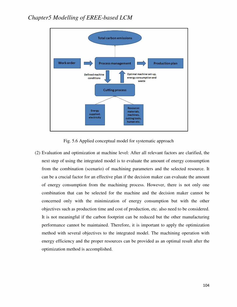
Chapter5 Modelling of EREE-based LCM
104
Fig. 5.6 Applied conceptual model for systematic approach
(2) Evaluation and optimization at machine level: After all relevant factors are clarified, the
next step of using the integrated model is to evaluate the amount of energy consumption
from the combination (scenario) of machining parameters and the selected resource. It
can be a crucial factor for an effective plan if the decision maker can evaluate the amount
of energy consumption from the machining process. However, there is not only one
combination that can be selected for the machine and the decision maker cannot be
concerned only with the minimization of energy consumption but with the other
objectives such as production time and cost of production, etc. also need to be considered.
It is not meaningful if the carbon footprint can be reduced but the other manufacturing
performance cannot be maintained. Therefore, it is important to apply the optimization
method with several objectives to the integrated model. The machining operation with
energy efficiency and the proper resources can be provided as an optimal result after the
optimization method is accomplished.
Chapter5 Modelling of EREE-based LCM
105
(3) Waste minimization at machine level: This is the final step at machine level regarding the
conceptual model when energy efficiency and resource utilization are already determined
respectively. All causes that can waste energy and the carbon footprint from the machine
must be considered such as idle time, break down time, tool life and operator error etc.
Therefore, the history or record of waste that relate to the optimal solution (scenario)
from the previous section must be prepared. In order to complete at this stage, the author
uses the discrete event simulation method to observe waste that occurs during the
manufacturing process and calculate the total waste of the carbon footprint. From the
simulation results, the preventive plan is possibly planed in advance to eliminate the
waste of carbon footprint. Therefore, the decision maker can choose the optimal solution
with a preventive plan which eventually refers to low carbon manufacturing machine
level.
(4) Understanding the system flow of the considered shop-floor: This stage is going deeper in
terms of complexity as it is a higher level of the manufacturing system. There is not only
one machine to be considered like at machine level but there are many machines located
in different places regarding to the shop-floor layout. In an everyday situation, there
could be many types of workpiece or product that are required to be machined on the
shop-floor. Some products can be machined with any machines while some products need
a specific group of machines. In addition, different products have different process
sequences. With these details, it is obvious that all information related to the considered
shop-floor such as machine capacity, objective requirements, process chain details, lists
of machines and products, cycle time, maintenance down time, shift assignment for
worker and product arrival time etc. must be prepared for the decision maker.
(5) Optimization for energy efficiency and resource utilization at shop-floor level: According
to the details from the previous section, the optimization model for the operation plan
must be established at this stage. This step is similar to the second step when objectives
and goals are concerned with the formulation of the optimization model. In the real
world, there is normally more than one goal or objective that must be satisfied at the same
time per planning. So, the establishment of a multi objective operational model which is
subjected to all system constraints is very important at this step. For the evaluation of

Chapter5 Modelling of EREE-based LCM
106
energy consumption from the machining process, all machines in the system have used
the methodologies in the second step of the machine level. So, the data of energy
consumption can be prepared by this way. The work assignment plan and proper selected
resource (machine, cutting tool and operator) with energy efficiency can be provided after
the optimal solution is obtained. All machines can also be operated with optimal setting
when the machine level was applied with the proposed model before. This is the
advantage of allying the systematic approach.
(6) Waste minimization at shop-floor level: Even though, the optimal solution from the
optimization method returns the used of energy efficiency regarding the results, the real
energy consumption and carbon footprint might be higher than the level it should be. This
is also similar to the case at machine level. However, the number of machines on the
shop-floor is too many compared to the machine level (only one). This means the amount
of waste energy consumption and carbon footprint must be much more as well and the
optimal solution will not be meaningful. Hence, the process for waste minimization is
also important at shop-floor level. The author uses the same technique as described in the
third step. More numerical examples will be presented in the applications and discussion
section.
5.6 EREE-based LCM at the machine level
5.6.1 The cutting force system
In the machining process, the relationship between the cutting force system and chip load is often
mentioned. In Fig. 5.7, it depicts the conventional dynamic end milling cutting force prediction
model and its relationship in the form of a feedback control diagram. The cutting force system
can be expressed in the function of the contact area between the end mill and workpiece (chip
load). A model for chip load determination is formulated as a function of process geometry.
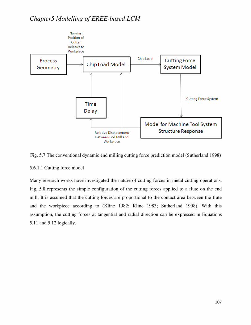
Chapter5 Modelling of EREE-based LCM
107
Fig. 5.7 The conventional dynamic end milling cutting force prediction model (Sutherland 1998)
5.6.1.1 Cutting force model
Many research works have investigated the nature of cutting forces in metal cutting operations.
Fig. 5.8 represents the simple configuration of the cutting forces applied to a flute on the end
mill. It is assumed that the cutting forces are proportional to the contact area between the flute
and the workpiece according to (Kline 1982; Kline 1983; Sutherland 1998). With this
assumption, the cutting forces at tangential and radial direction can be expressed in Equations
5.11 and 5.12 logically.
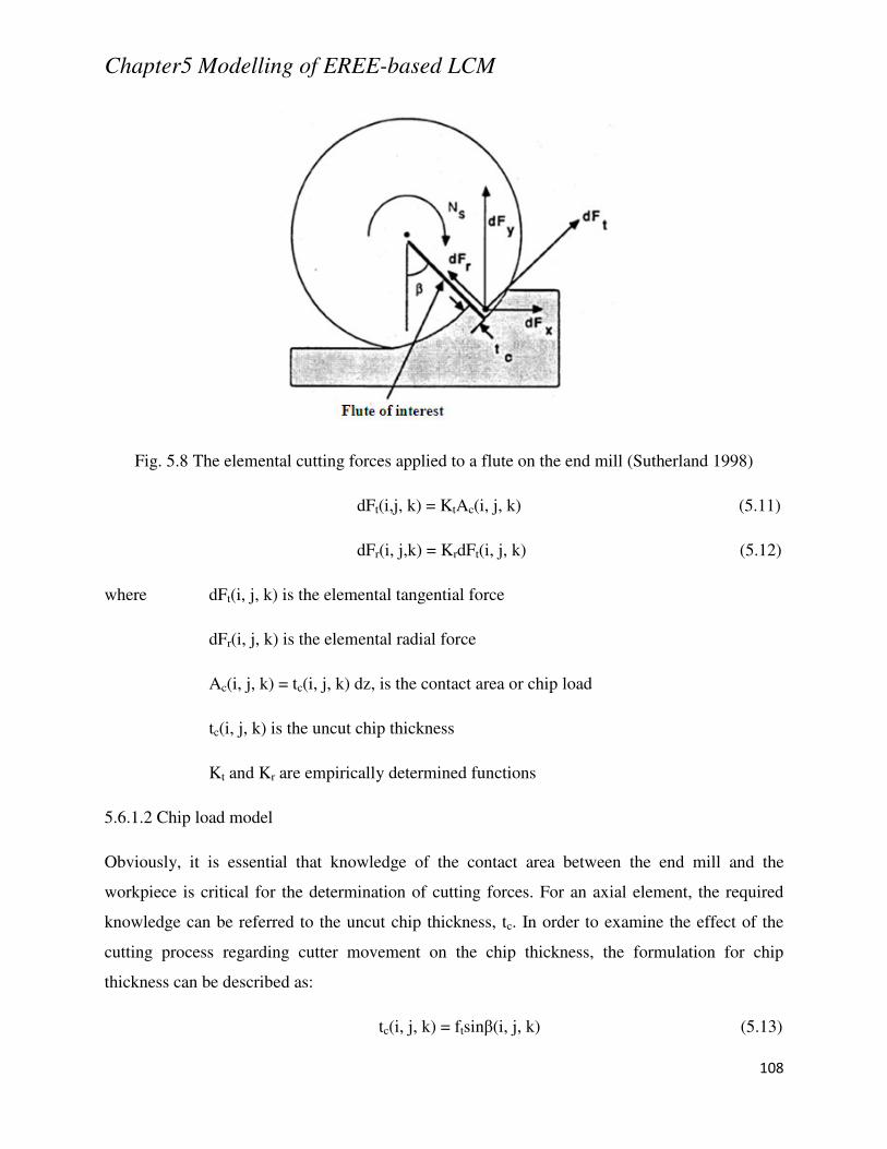
Chapter5 Modelling of EREE-based LCM
108
Fig. 5.8 The elemental cutting forces applied to a flute on the end mill (Sutherland 1998)
dFt(i,j, k) = KtAc(i, j, k) (5.11)
dFr(i, j,k) = KrdFt(i, j, k) (5.12)
where dFt(i, j, k) is the elemental tangential force
dFr(i, j, k) is the elemental radial force
Ac(i, j, k) = tc(i, j, k) dz, is the contact area or chip load
tc(i, j, k) is the uncut chip thickness
Kt and Kr are empirically determined functions
5.6.1.2 Chip load model
Obviously, it is essential that knowledge of the contact area between the end mill and the
workpiece is critical for the determination of cutting forces. For an axial element, the required
knowledge can be referred to the uncut chip thickness, tc. In order to examine the effect of the
cutting process regarding cutter movement on the chip thickness, the formulation for chip
thickness can be described as:
tc(i, j, k) = ftsinβ(i, j, k) (5.13)
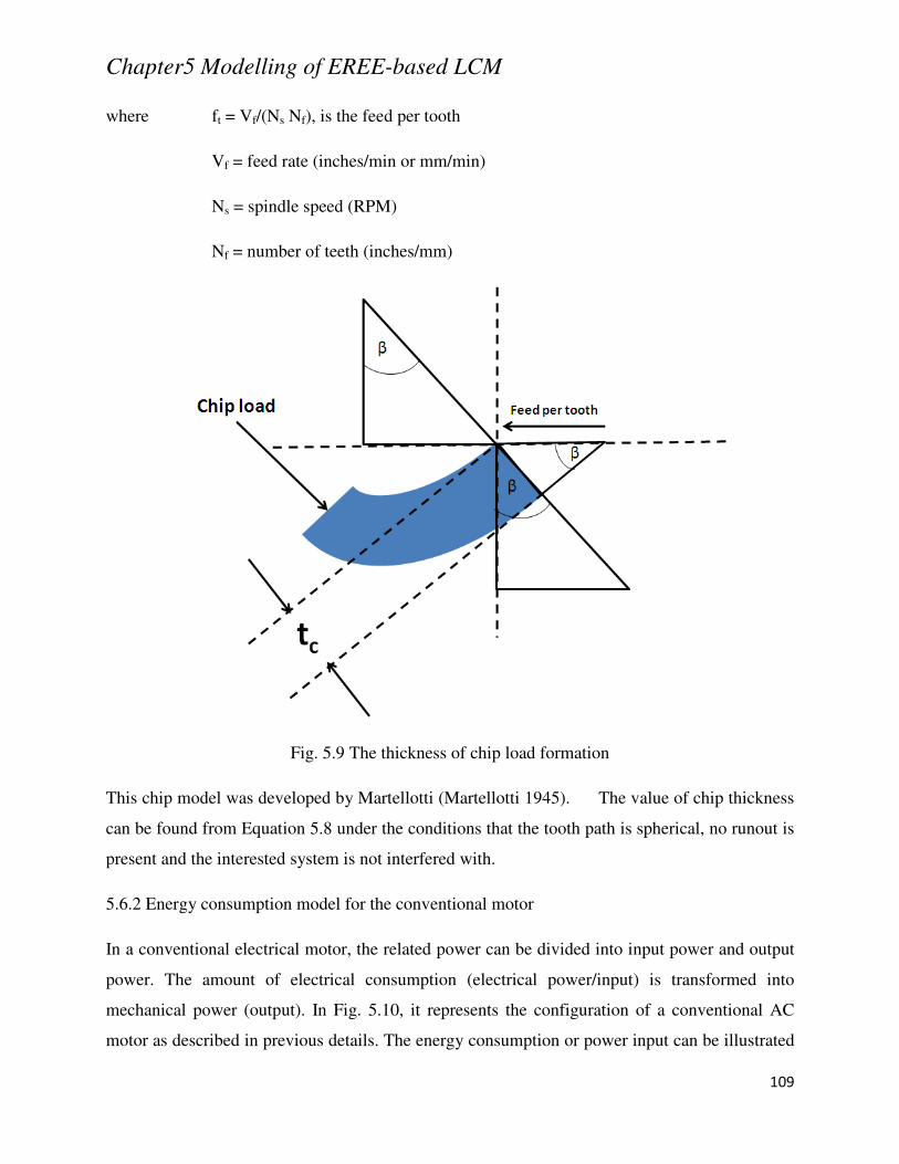
Chapter5 Modelling of EREE-based LCM
109
where ft = Vf/(Ns Nf), is the feed per tooth
Vf = feed rate (inches/min or mm/min)
Ns = spindle speed (RPM)
Nf = number of teeth (inches/mm)
Fig. 5.9 The thickness of chip load formation
This chip model was developed by Martellotti (Martellotti 1945). The value of chip thickness
can be found from Equation 5.8 under the conditions that the tooth path is spherical, no runout is
present and the interested system is not interfered with.
5.6.2 Energy consumption model for the conventional motor
In a conventional electrical motor, the related power can be divided into input power and output
power. The amount of electrical consumption (electrical power/input) is transformed into
mechanical power (output). In Fig. 5.10, it represents the configuration of a conventional AC
motor as described in previous details. The energy consumption or power input can be illustrated
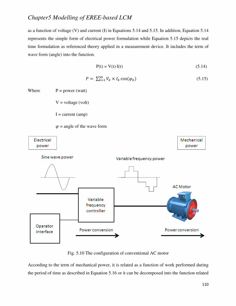
Chapter5 Modelling of EREE-based LCM
110
as a function of voltage (V) and current (I) in Equations 5.14 and 5.15. In addition, Equation 5.14
represents the simple form of electrical power formulation while Equation 5.15 depicts the real
time formulation as referenced theory applied in a measurement device. It includes the term of
wave form (angle) into the function.
P(t) = V(t)·I(t) (5.14)
∑ R S TR cosRXYRZ (5.15)
Where P = power (watt)
V = voltage (volt)
I = current (amp)
= angle of the wave form
Fig. 5.10 The configuration of conventional AC motor
According to the term of mechanical power, it is related as a function of work performed during
the period of time as described in Equation 5.16 or it can be decomposed into the function related
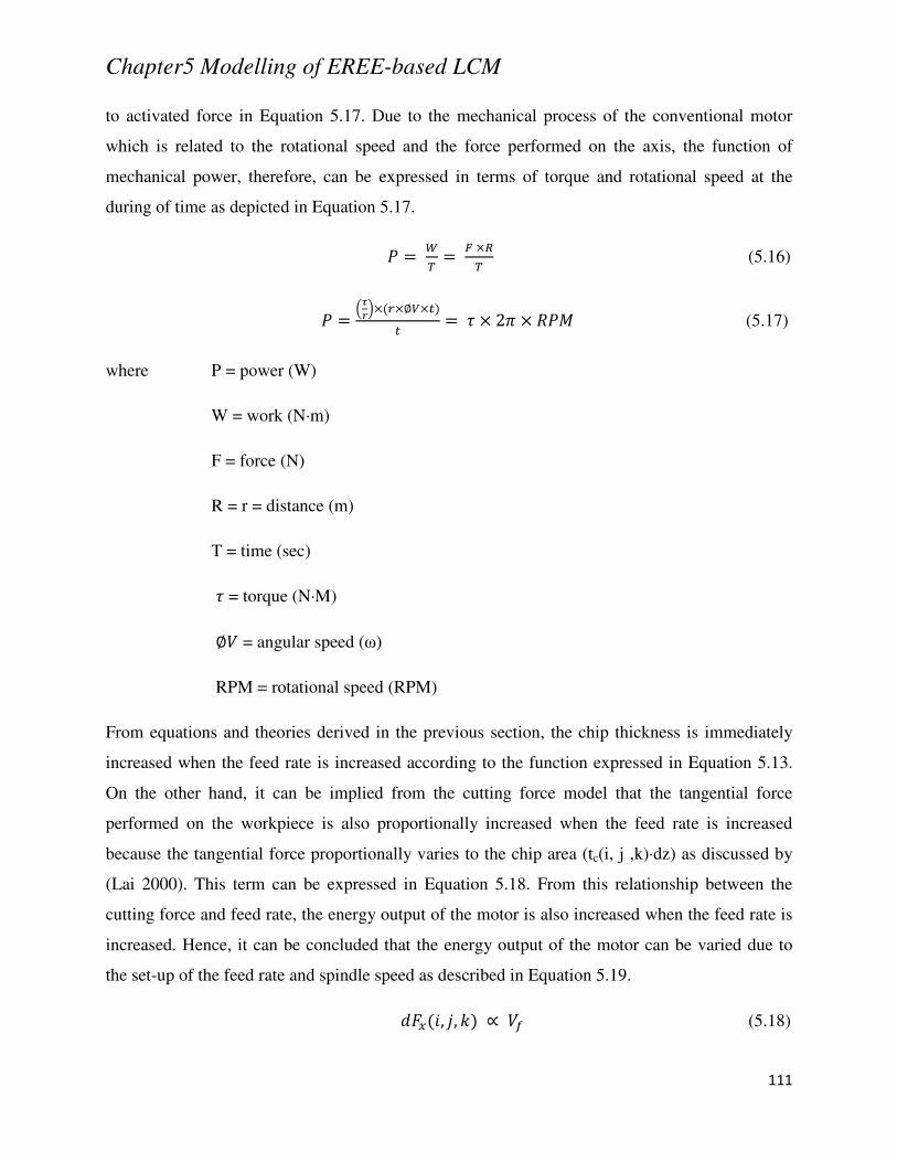
Chapter5 Modelling of EREE-based LCM
111
to activated force in Equation 5.17. Due to the mechanical process of the conventional motor
which is related to the rotational speed and the force performed on the axis, the function of
mechanical power, therefore, can be expressed in terms of torque and rotational speed at the
during of time as depicted in Equation 5.17.
[\ ] S^\ (5.16)
_abS$ScS S 2d S e (5.17)
where P = power (W)
W = work (N·m)
F = force (N)
R = r = distance (m)
T = time (sec)
= torque (N·M)
= angular speed (ω)
RPM = rotational speed (RPM)
From equations and theories derived in the previous section, the chip thickness is immediately
increased when the feed rate is increased according to the function expressed in Equation 5.13.
On the other hand, it can be implied from the cutting force model that the tangential force
performed on the workpiece is also proportionally increased when the feed rate is increased
because the tangential force proportionally varies to the chip area (tc(i, j ,k)·dz) as discussed by
(Lai 2000). This term can be expressed in Equation 5.18. From this relationship between the
cutting force and feed rate, the energy output of the motor is also increased when the feed rate is
increased. Hence, it can be concluded that the energy output of the motor can be varied due to
the set-up of the feed rate and spindle speed as described in Equation 5.19.
O f, g, h C . (5.18)
Chapter5 Modelling of EREE-based LCM
112
C . , e (5.19)
In Fig. 5.11 and fig. 5.12, the energy consumption data from cutting trials using the commercial
CNC turning machine are presented. It is obvious that the energy input (electrical energy) is
increased when the machine parameters including spindle speed, feed rate and depth of cut are
increased. In addition, it can be implied that the energy input is proportional with the energy
output. Therefore, the relationship between machining parameters and the amount of energy
consumption can be expressed in Equation 5.20.
",-' C &'-' C ., e (5.20)
Fig. 5.11 Cutting trial under the conditions: 2500 rpm, 1000 mm/min and 1 mm
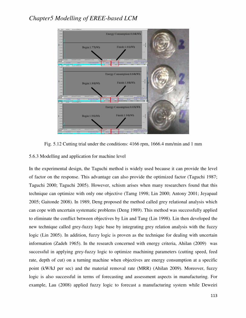
Chapter5 Modelling of EREE-based LCM
113
Fig. 5.12 Cutting trial under the conditions: 4166 rpm, 1666.4 mm/min and 1 mm
5.6.3 Modelling and application for machine level
In the experimental design, the Taguchi method is widely used because it can provide the level
of factor on the response. This advantage can also provide the optimized factor (Taguchi 1987;
Taguchi 2000; Taguchi 2005). However, schism arises when many researchers found that this
technique can optimize with only one objective (Tarng 1998; Lin 2000; Antony 2001; Jeyapaul
2005; Gaitonde 2008). In 1989, Deng proposed the method called grey relational analysis which
can cope with uncertain systematic problems (Deng 1989). This method was successfully applied
to eliminate the conflict between objectives by Lin and Tang (Lin 1998). Lin then developed the
new technique called grey-fuzzy logic base by integrating grey relation analysis with the fuzzy
logic (Lin 2005). In addition, fuzzy logic is proven as the technique for dealing with uncertain
information (Zadeh 1965). In the research concerned with energy criteria, Ahilan (2009) was
successful in applying grey-fuzzy logic to optimize machining parameters (cutting speed, feed
rate, depth of cut) on a turning machine when objectives are energy consumption at a specific
point (kW/kJ per sec) and the material removal rate (MRR) (Ahilan 2009). Moreover, fuzzy
logic is also successful in terms of forecasting and assessment aspects in manufacturing. For
example, Lau (2008) applied fuzzy logic to forecast a manufacturing system while Deweiri

Chapter5 Modelling of EREE-based LCM
114
(2003) used fuzzy logic to generate surface roughness in the milling process (Dweiri 2003; Lau
2008).
Whilst the grey-fuzzy reasoning grade method is successful in different manufacturing processes
(Lin 1998; Lin 2005), the ability to predict and optimize the input parameters which exclude
from experimental results is limited. For example, the experiment runs with two levels of depth
of cut (1mm and 3mm) on the cutting trial. The grey-fuzzy reasoning grade can only select these
two values for the optimization process. Therefore, the development of the effective system
which can also predict the total energy consumption together with the optimization process is
necessary for flexible planning on CNC machining.
In this section, the developed model for EREE-based LCM for the machine level is proposed.
The model aims to provide optimal machine operations with energy efficiency, proper resource
utilization and waste minimization for the decision maker. The model is illustrated in Fig. 5.13.
The model begins with the evaluation of energy consumption when cutter parameters and
selected resources are prepared. Then, the optimization model seeks the optimal combinations of
machine set-up that can compromise with all desired objectives based on the optimized rules.
Finally, the related waste data is provided for the optimal machine set-up. The simulation can be
used to prevent waste occurring after the selected machining set-up was used.
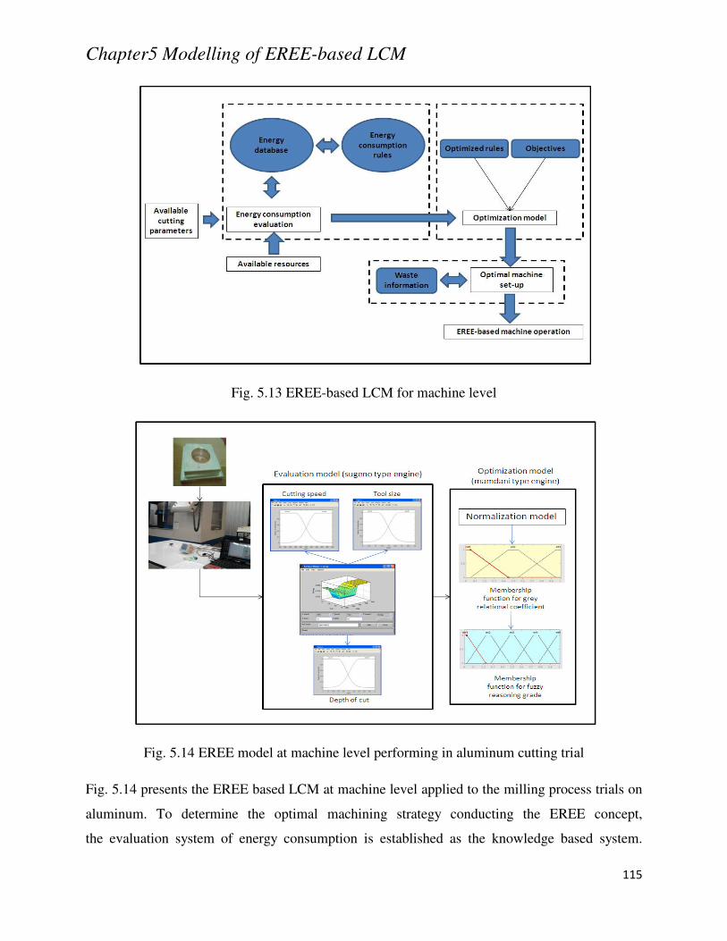
Chapter5 Modelling of EREE-based LCM
115
Fig. 5.13 EREE-based LCM for machine level
Fig. 5.14 EREE model at machine level performing in aluminum cutting trial
Fig. 5.14 presents the EREE based LCM at machine level applied to the milling process trials on
aluminum. To determine the optimal machining strategy conducting the EREE concept,
the evaluation system of energy consumption is established as the knowledge based system.
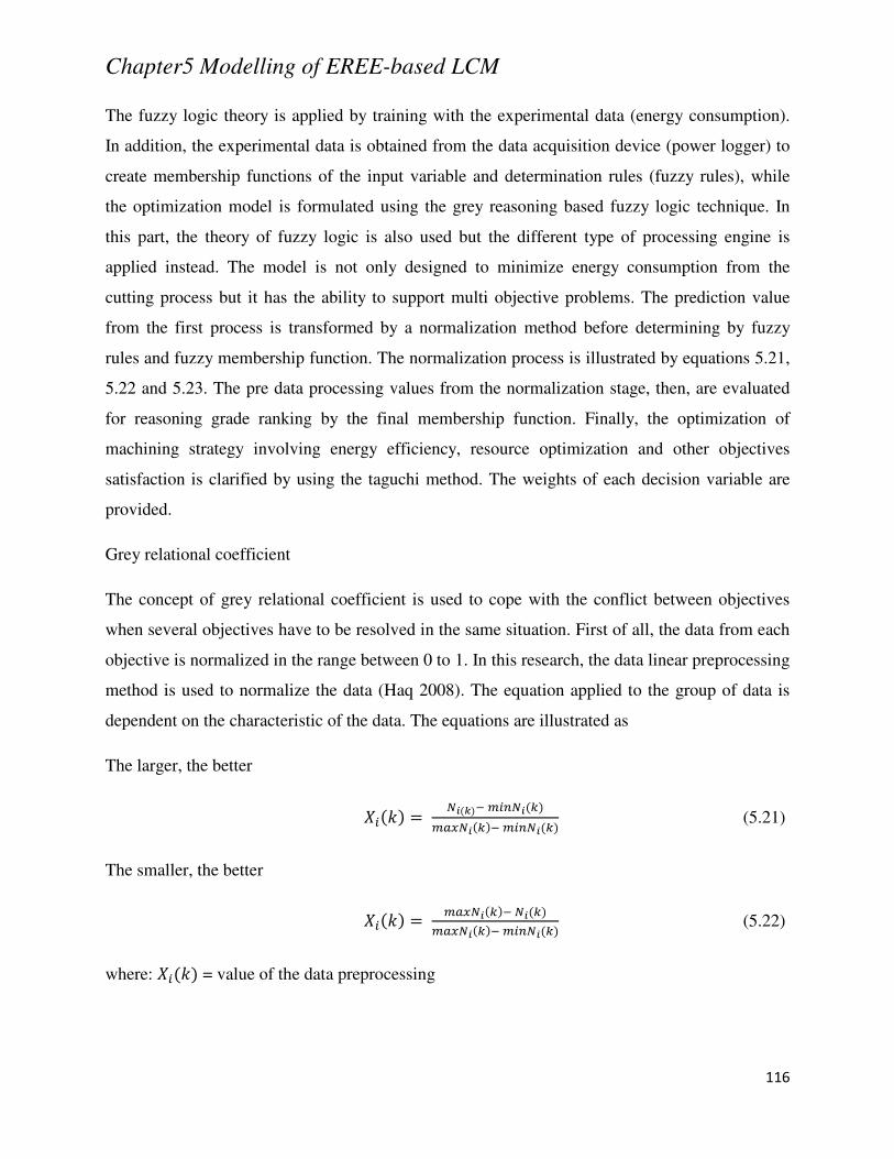
Chapter5 Modelling of EREE-based LCM
116
The fuzzy logic theory is applied by training with the experimental data (energy consumption).
In addition, the experimental data is obtained from the data acquisition device (power logger) to
create membership functions of the input variable and determination rules (fuzzy rules), while
the optimization model is formulated using the grey reasoning based fuzzy logic technique. In
this part, the theory of fuzzy logic is also used but the different type of processing engine is
applied instead. The model is not only designed to minimize energy consumption from the
cutting process but it has the ability to support multi objective problems. The prediction value
from the first process is transformed by a normalization method before determining by fuzzy
rules and fuzzy membership function. The normalization process is illustrated by equations 5.21,
5.22 and 5.23. The pre data processing values from the normalization stage, then, are evaluated
for reasoning grade ranking by the final membership function. Finally, the optimization of
machining strategy involving energy efficiency, resource optimization and other objectives
satisfaction is clarified by using the taguchi method. The weights of each decision variable are
provided.
Grey relational coefficient
The concept of grey relational coefficient is used to cope with the conflict between objectives
when several objectives have to be resolved in the same situation. First of all, the data from each
objective is normalized in the range between 0 to 1. In this research, the data linear preprocessing
method is used to normalize the data (Haq 2008). The equation applied to the group of data is
dependent on the characteristic of the data. The equations are illustrated as
The larger, the better
1"h ?ijk #",?iR#*f?iRk #",?iR (5.21)
The smaller, the better
1"h #*f?iRk ?iR#*f?iRk #",?iR (5.22)
where: 1"h = value of the data preprocessing
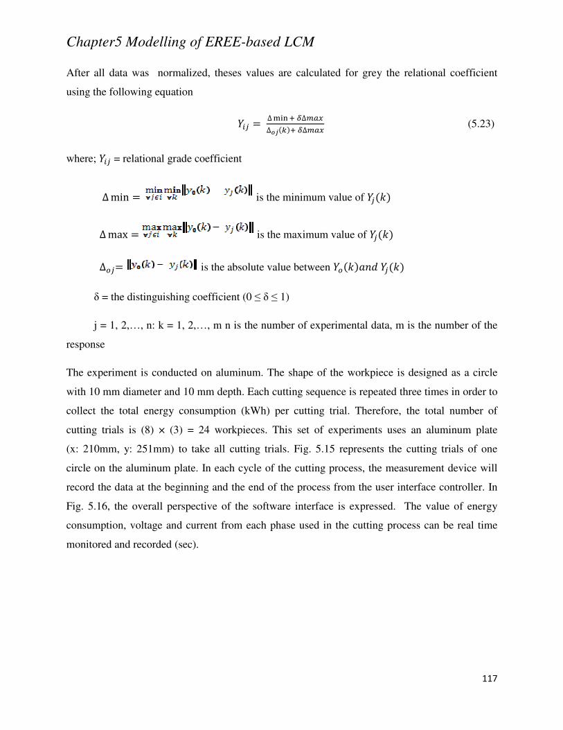
Chapter5 Modelling of EREE-based LCM
117
After all data was normalized, theses values are calculated for grey the relational coefficient
using the following equation
2"l ∆nopq r∆#*f∆stRq r∆#*f (5.23)
where; 2"l = relational grade coefficient
∆min is the minimum value of 2lh ∆max is the maximum value of 2lh ∆&l is the absolute value between 2&hO 2lh δ = the distinguishing coefficient (0 ≤ δ ≤ 1)
j = 1, 2,…, n: k = 1, 2,…, m n is the number of experimental data, m is the number of the
response
The experiment is conducted on aluminum. The shape of the workpiece is designed as a circle
with 10 mm diameter and 10 mm depth. Each cutting sequence is repeated three times in order to
collect the total energy consumption (kWh) per cutting trial. Therefore, the total number of
cutting trials is (8) × (3) = 24 workpieces. This set of experiments uses an aluminum plate
(x: 210mm, y: 251mm) to take all cutting trials. Fig. 5.15 represents the cutting trials of one
circle on the aluminum plate. In each cycle of the cutting process, the measurement device will
record the data at the beginning and the end of the process from the user interface controller. In
Fig. 5.16, the overall perspective of the software interface is expressed. The value of energy
consumption, voltage and current from each phase used in the cutting process can be real time
monitored and recorded (sec).
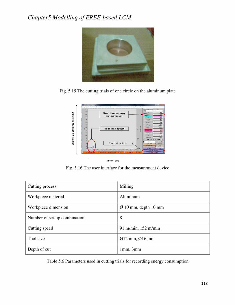
Chapter5 Modelling of EREE-based LCM
118
Fig. 5.15 The cutting trials of one circle on the aluminum plate
Fig. 5.16 The user interface for the measurement device
Cutting process Milling
Workpiece material Aluminum
Workpiece dimension Ø 10 mm, depth 10 mm
Number of set-up combination 8
Cutting speed 91 m/min, 152 m/min
Tool size Ø12 mm, Ø16 mm
Depth of cut 1mm, 3mm
Table 5.6 Parameters used in cutting trials for recording energy consumption
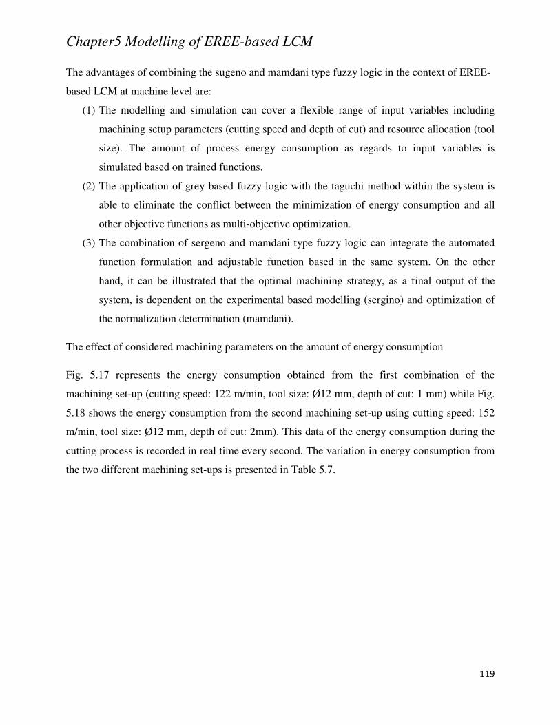
Chapter5 Modelling of EREE-based LCM
119
The advantages of combining the sugeno and mamdani type fuzzy logic in the context of EREE-
based LCM at machine level are:
(1) The modelling and simulation can cover a flexible range of input variables including
machining setup parameters (cutting speed and depth of cut) and resource allocation (tool
size). The amount of process energy consumption as regards to input variables is
simulated based on trained functions.
(2) The application of grey based fuzzy logic with the taguchi method within the system is
able to eliminate the conflict between the minimization of energy consumption and all
other objective functions as multi-objective optimization.
(3) The combination of sergeno and mamdani type fuzzy logic can integrate the automated
function formulation and adjustable function based in the same system. On the other
hand, it can be illustrated that the optimal machining strategy, as a final output of the
system, is dependent on the experimental based modelling (sergino) and optimization of
the normalization determination (mamdani).
The effect of considered machining parameters on the amount of energy consumption
Fig. 5.17 represents the energy consumption obtained from the first combination of the
machining set-up (cutting speed: 122 m/min, tool size: Ø12 mm, depth of cut: 1 mm) while Fig.
5.18 shows the energy consumption from the second machining set-up using cutting speed: 152
m/min, tool size: Ø12 mm, depth of cut: 2mm). This data of the energy consumption during the
cutting process is recorded in real time every second. The variation in energy consumption from
the two different machining set-ups is presented in Table 5.7.
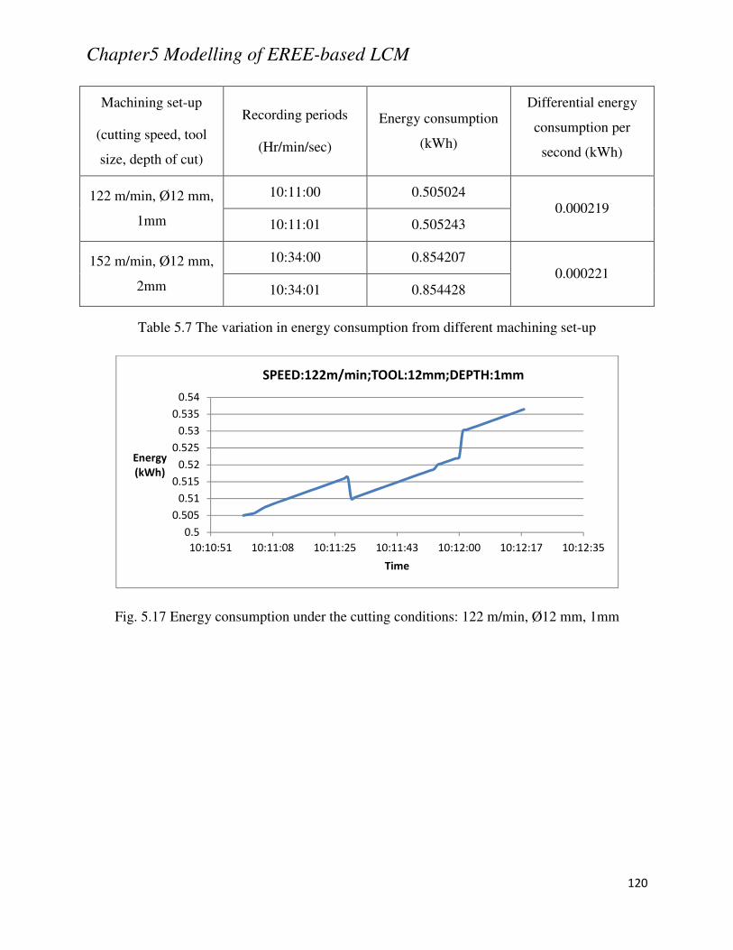
Chapter5 Modelling of EREE-based LCM
120
Machining set-up
(cutting speed, tool
size, depth of cut)
Recording periods
(Hr/min/sec)
Energy consumption
(kWh)
Differential energy
consumption per
second (kWh)
122 m/min, Ø12 mm,
1mm
10:11:00 0.505024 0.000219
10:11:01 0.505243
152 m/min, Ø12 mm,
2mm
10:34:00 0.854207 0.000221
10:34:01 0.854428
Table 5.7 The variation in energy consumption from different machining set-up
Fig. 5.17 Energy consumption under the cutting conditions: 122 m/min, Ø12 mm, 1mm
0.5
0.505
0.51
0.515
0.52
0.525
0.53
0.535
0.54
10:10:51 10:11:08 10:11:25 10:11:43 10:12:00 10:12:17 10:12:35
Energy
(kWh)
Time
SPEED:122m/min;TOOL:12mm;DEPTH:1mm
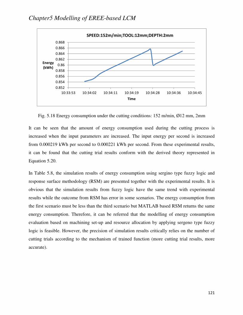
Chapter5 Modelling of EREE-based LCM
121
Fig. 5.18 Energy consumption under the cutting conditions: 152 m/min, Ø12 mm, 2mm
It can be seen that the amount of energy consumption used during the cutting process is
increased when the input parameters are increased. The input energy per second is increased
from 0.000219 kWh per second to 0.000221 kWh per second. From these experimental results,
it can be found that the cutting trial results conform with the derived theory represented in
Equation 5.20.
In Table 5.8, the simulation results of energy consumption using sergino type fuzzy logic and
response surface methodology (RSM) are presented together with the experimental results. It is
obvious that the simulation results from fuzzy logic have the same trend with experimental
results while the outcome from RSM has error in some scenarios. The energy consumption from
the first scenario must be less than the third scenario but MATLAB based RSM returns the same
energy consumption. Therefore, it can be referred that the modelling of energy consumption
evaluation based on machining set-up and resource allocation by applying sergeno type fuzzy
logic is feasible. However, the precision of simulation results critically relies on the number of
cutting trials according to the mechanism of trained function (more cutting trial results, more
accurate).
0.852
0.854
0.856
0.858
0.86
0.862
0.864
0.866
0.868
10:33:53 10:34:02 10:34:11 10:34:19 10:34:28 10:34:36 10:34:45
Energy
(kWh)
Time
SPEED:152m/min;TOOL:12mm;DEPTH:2mm
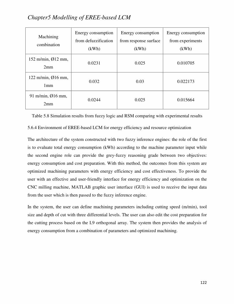
Chapter5 Modelling of EREE-based LCM
122
Machining
combination
Energy consumption
from defuzzification
(kWh)
Energy consumption
from response surface
(kWh)
Energy consumption
from experiments
(kWh)
152 m/min, Ø12 mm,
2mm 0.0231 0.025 0.010705
122 m/min, Ø16 mm,
1mm 0.032 0.03 0.022173
91 m/min, Ø16 mm,
2mm 0.0244 0.025 0.015664
Table 5.8 Simulation results from fuzzy logic and RSM comparing with experimental results
5.6.4 Environment of EREE-based LCM for energy efficiency and resource optimization
The architecture of the system constructed with two fuzzy inference engines: the role of the first
is to evaluate total energy consumption (kWh) according to the machine parameter input while
the second engine role can provide the grey-fuzzy reasoning grade between two objectives:
energy consumption and cost preparation. With this method, the outcomes from this system are
optimized machining parameters with energy efficiency and cost effectiveness. To provide the
user with an effective and user-friendly interface for energy efficiency and optimization on the
CNC milling machine, MATLAB graphic user interface (GUI) is used to receive the input data
from the user which is then passed to the fuzzy inference engine.
In the system, the user can define machining parameters including cutting speed (m/min), tool
size and depth of cut with three differential levels. The user can also edit the cost preparation for
the cutting process based on the L9 orthogonal array. The system then provides the analysis of
energy consumption from a combination of parameters and optimized machining.
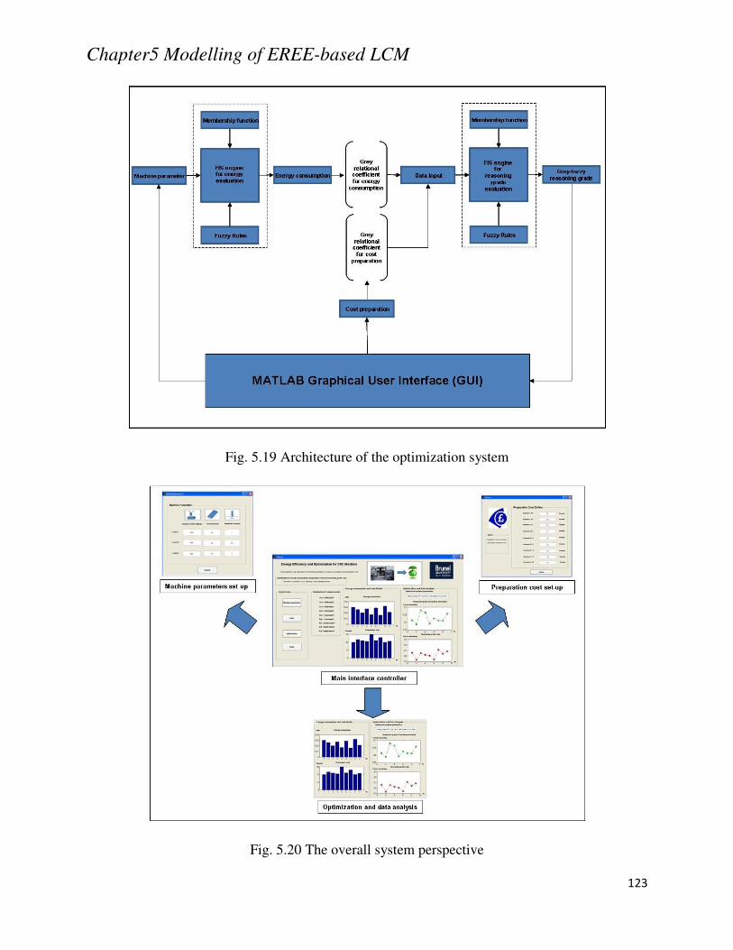
Chapter5 Modelling of EREE-based LCM
123
Fig. 5.19 Architecture of the optimization system
Fig. 5.20 The overall system perspective
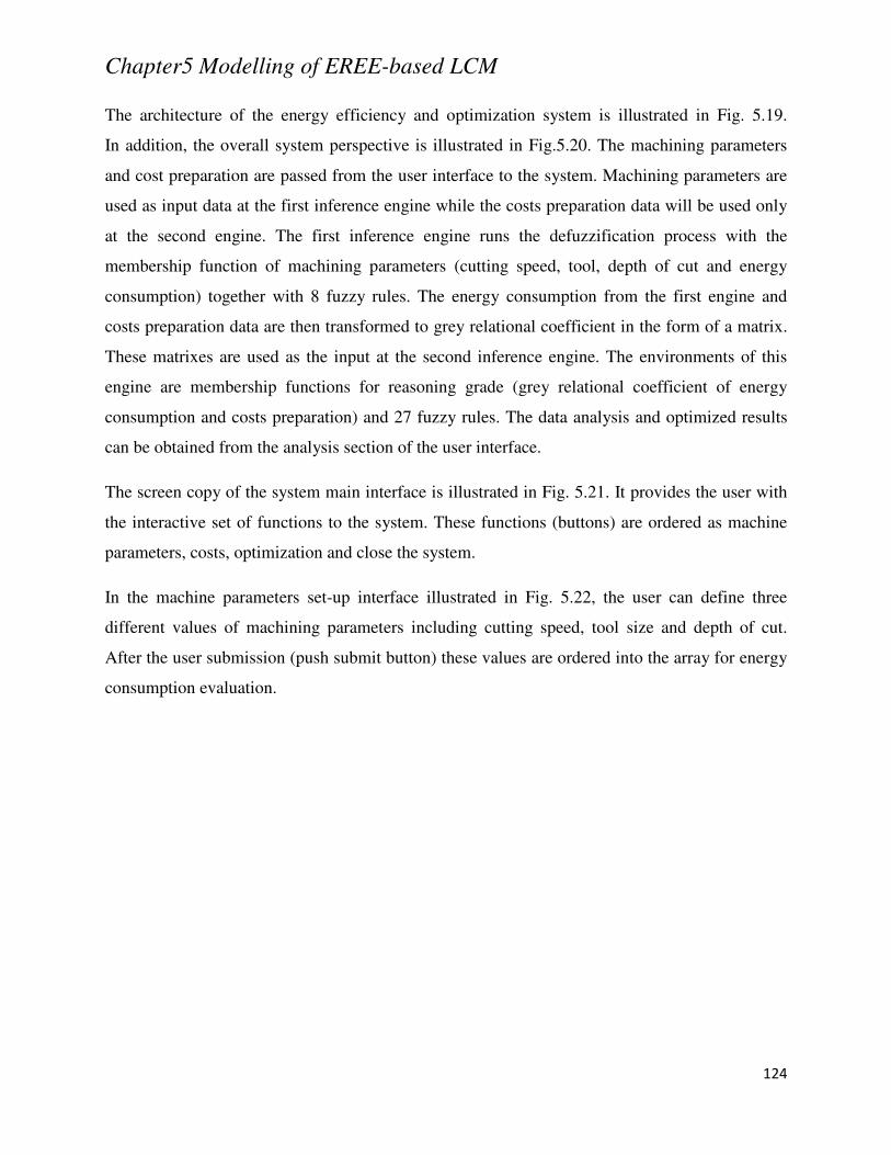
Chapter5 Modelling of EREE-based LCM
124
The architecture of the energy efficiency and optimization system is illustrated in Fig. 5.19.
In addition, the overall system perspective is illustrated in Fig.5.20. The machining parameters
and cost preparation are passed from the user interface to the system. Machining parameters are
used as input data at the first inference engine while the costs preparation data will be used only
at the second engine. The first inference engine runs the defuzzification process with the
membership function of machining parameters (cutting speed, tool, depth of cut and energy
consumption) together with 8 fuzzy rules. The energy consumption from the first engine and
costs preparation data are then transformed to grey relational coefficient in the form of a matrix.
These matrixes are used as the input at the second inference engine. The environments of this
engine are membership functions for reasoning grade (grey relational coefficient of energy
consumption and costs preparation) and 27 fuzzy rules. The data analysis and optimized results
can be obtained from the analysis section of the user interface.
The screen copy of the system main interface is illustrated in Fig. 5.21. It provides the user with
the interactive set of functions to the system. These functions (buttons) are ordered as machine
parameters, costs, optimization and close the system.
In the machine parameters set-up interface illustrated in Fig. 5.22, the user can define three
different values of machining parameters including cutting speed, tool size and depth of cut.
After the user submission (push submit button) these values are ordered into the array for energy
consumption evaluation.
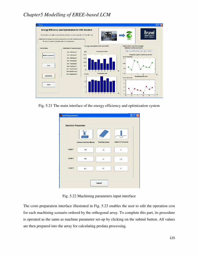
Chapter5 Modelling of EREE-based LCM
125
Fig. 5.21 The main interface of the energy efficiency and optimization system
Fig. 5.22 Machining parameters input interface
The costs preparation interface illustrated in Fig. 5.23 enables the user to edit the operation cost
for each machining scenario ordered by the orthogonal array. To complete this part, its procedure
is operated as the same as machine parameter set-up by clicking on the submit button. All values
are then prepared into the array for calculating predata processing.
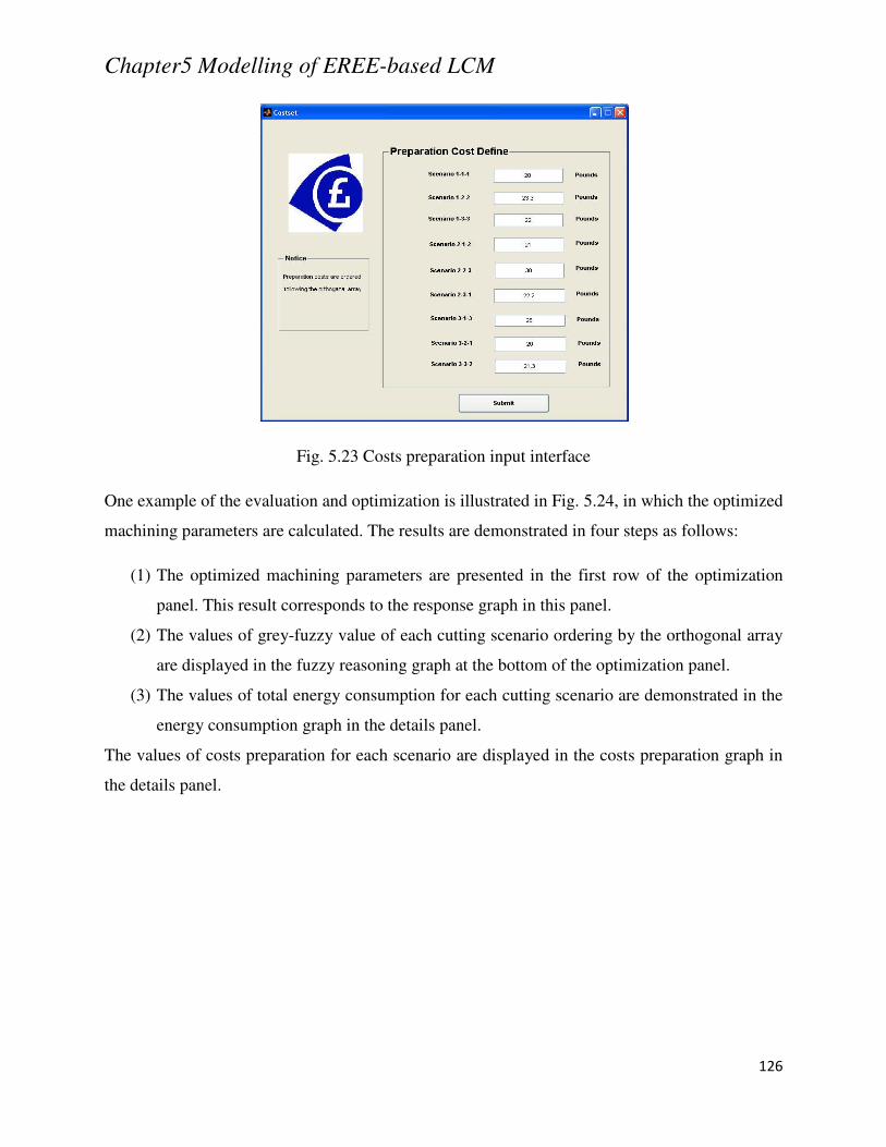
Chapter5 Modelling of EREE-based LCM
126
Fig. 5.23 Costs preparation input interface
One example of the evaluation and optimization is illustrated in Fig. 5.24, in which the optimized
machining parameters are calculated. The results are demonstrated in four steps as follows:
(1) The optimized machining parameters are presented in the first row of the optimization
panel. This result corresponds to the response graph in this panel.
(2) The values of grey-fuzzy value of each cutting scenario ordering by the orthogonal array
are displayed in the fuzzy reasoning graph at the bottom of the optimization panel.
(3) The values of total energy consumption for each cutting scenario are demonstrated in the
energy consumption graph in the details panel.
The values of costs preparation for each scenario are displayed in the costs preparation graph in
the details panel.
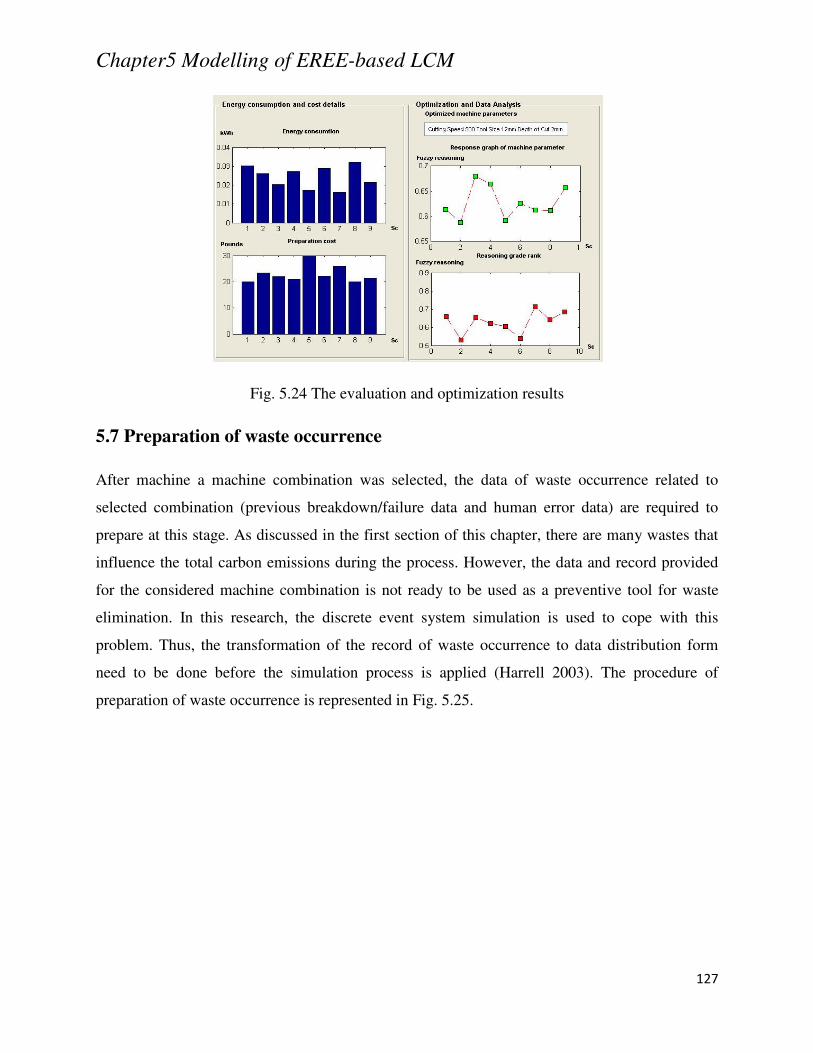
Chapter5 Modelling of EREE-based LCM
127
Fig. 5.24 The evaluation and optimization results
5.7 Preparation of waste occurrence
After machine a machine combination was selected, the data of waste occurrence related to
selected combination (previous breakdown/failure data and human error data) are required to
prepare at this stage. As discussed in the first section of this chapter, there are many wastes that
influence the total carbon emissions during the process. However, the data and record provided
for the considered machine combination is not ready to be used as a preventive tool for waste
elimination. In this research, the discrete event system simulation is used to cope with this
problem. Thus, the transformation of the record of waste occurrence to data distribution form
need to be done before the simulation process is applied (Harrell 2003). The procedure of
preparation of waste occurrence is represented in Fig. 5.25.
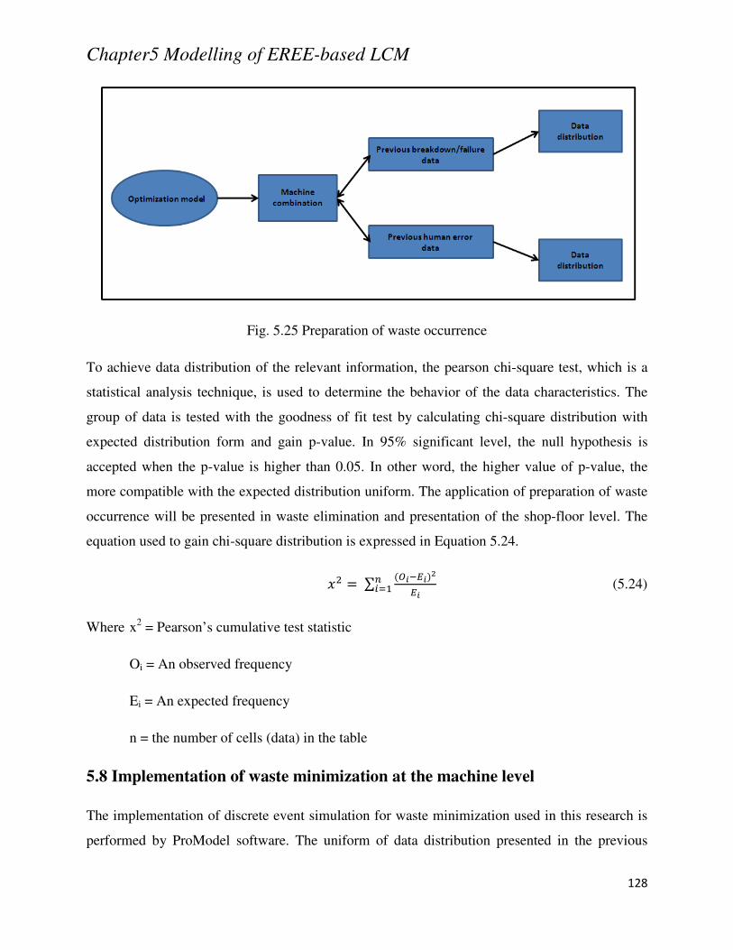
Chapter5 Modelling of EREE-based LCM
128
Fig. 5.25 Preparation of waste occurrence
To achieve data distribution of the relevant information, the pearson chi-square test, which is a
statistical analysis technique, is used to determine the behavior of the data characteristics. The
group of data is tested with the goodness of fit test by calculating chi-square distribution with
expected distribution form and gain p-value. In 95% significant level, the null hypothesis is
accepted when the p-value is higher than 0.05. In other word, the higher value of p-value, the
more compatible with the expected distribution uniform. The application of preparation of waste
occurrence will be presented in waste elimination and presentation of the shop-floor level. The
equation used to gain chi-square distribution is expressed in Equation 5.24.
∑ ziki|i,"Z (5.24)
Where x2 = Pearson’s cumulative test statistic
Oi = An observed frequency
Ei = An expected frequency
n = the number of cells (data) in the table
5.8 Implementation of waste minimization at the machine level
The implementation of discrete event simulation for waste minimization used in this research is
performed by ProModel software. The uniform of data distribution presented in the previous
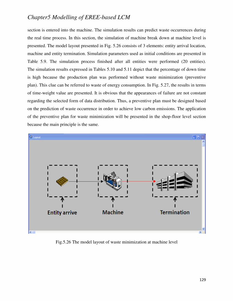
Chapter5 Modelling of EREE-based LCM
129
section is entered into the machine. The simulation results can predict waste occurrences during
the real time process. In this section, the simulation of machine break down at machine level is
presented. The model layout presented in Fig. 5.26 consists of 3 elements: entity arrival location,
machine and entity termination. Simulation parameters used as initial conditions are presented in
Table 5.9. The simulation process finished after all entities were performed (20 entities).
The simulation results expressed in Tables 5.10 and 5.11 depict that the percentage of down time
is high because the production plan was performed without waste minimization (preventive
plan). This clue can be referred to waste of energy consumption. In Fig. 5.27, the results in terms
of time-weight value are presented. It is obvious that the appearances of failure are not constant
regarding the selected form of data distribution. Thus, a preventive plan must be designed based
on the prediction of waste occurrence in order to achieve low carbon emissions. The application
of the preventive plan for waste minimization will be presented in the shop-floor level section
because the main principle is the same.
Fig.5.26 The model layout of waste minimization at machine level

Chapter5 Modelling of EREE-based LCM
130
Parameter setting Value
Processing time 5 min
Distribution of down time N(6,2)
Maintenance time 10 min
Inter arrival time of entity 10 min
Occurrence of entity 20
Table 5.9 Parameters for simulation set-up
Name
Scheduled
Time (HR) % Operation
%
Setup
%
Idle
%
Waiting
%
Blocked
%
Down
Loc1 3.83 43.48 0 4.35 0 0 52.17
Table 5.10 Percentage of machine down time
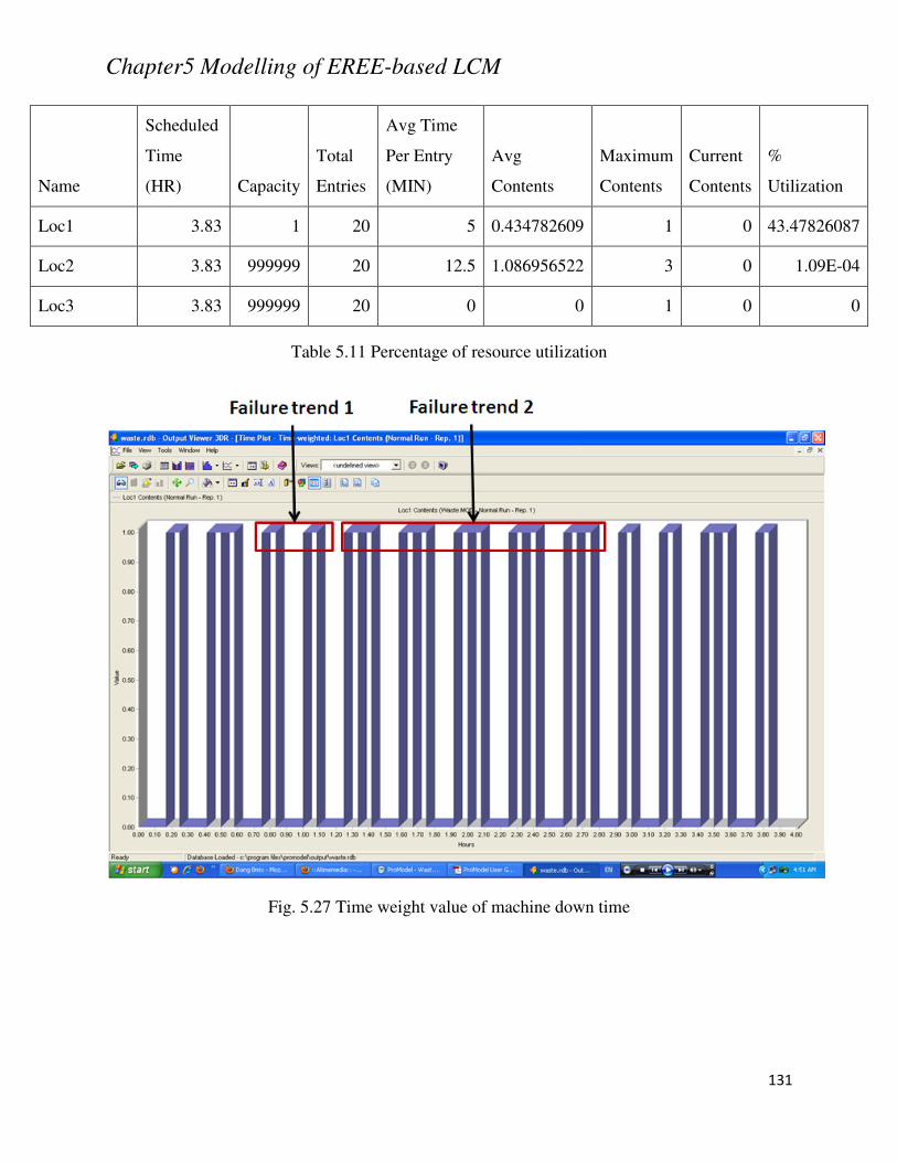
Chapter5 Modelling of EREE-based LCM
131
Name
Scheduled
Time
(HR) Capacity
Total
Entries
Avg Time
Per Entry
(MIN)
Avg
Contents
Maximum
Contents
Current
Contents
%
Utilization
Loc1 3.83 1 20 5 0.434782609 1 0 43.47826087
Loc2 3.83 999999 20 12.5 1.086956522 3 0 1.09E-04
Loc3 3.83 999999 20 0 0 1 0 0
Table 5.11 Percentage of resource utilization
Fig. 5.27 Time weight value of machine down time
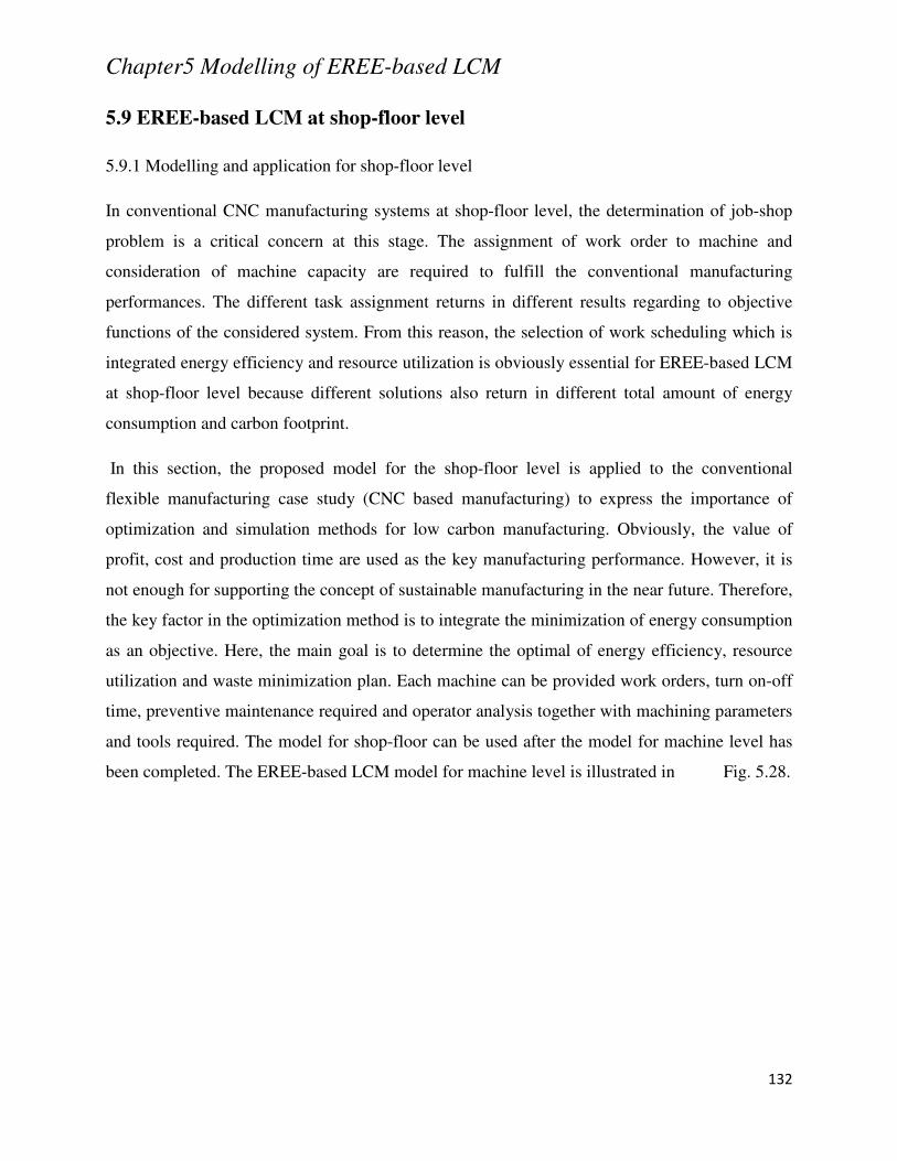
Chapter5 Modelling of EREE-based LCM
132
5.9 EREE-based LCM at shop-floor level
5.9.1 Modelling and application for shop-floor level
In conventional CNC manufacturing systems at shop-floor level, the determination of job-shop
problem is a critical concern at this stage. The assignment of work order to machine and
consideration of machine capacity are required to fulfill the conventional manufacturing
performances. The different task assignment returns in different results regarding to objective
functions of the considered system. From this reason, the selection of work scheduling which is
integrated energy efficiency and resource utilization is obviously essential for EREE-based LCM
at shop-floor level because different solutions also return in different total amount of energy
consumption and carbon footprint.
In this section, the proposed model for the shop-floor level is applied to the conventional
flexible manufacturing case study (CNC based manufacturing) to express the importance of
optimization and simulation methods for low carbon manufacturing. Obviously, the value of
profit, cost and production time are used as the key manufacturing performance. However, it is
not enough for supporting the concept of sustainable manufacturing in the near future. Therefore,
the key factor in the optimization method is to integrate the minimization of energy consumption
as an objective. Here, the main goal is to determine the optimal of energy efficiency, resource
utilization and waste minimization plan. Each machine can be provided work orders, turn on-off
time, preventive maintenance required and operator analysis together with machining parameters
and tools required. The model for shop-floor can be used after the model for machine level has
been completed. The EREE-based LCM model for machine level is illustrated in Fig. 5.28.
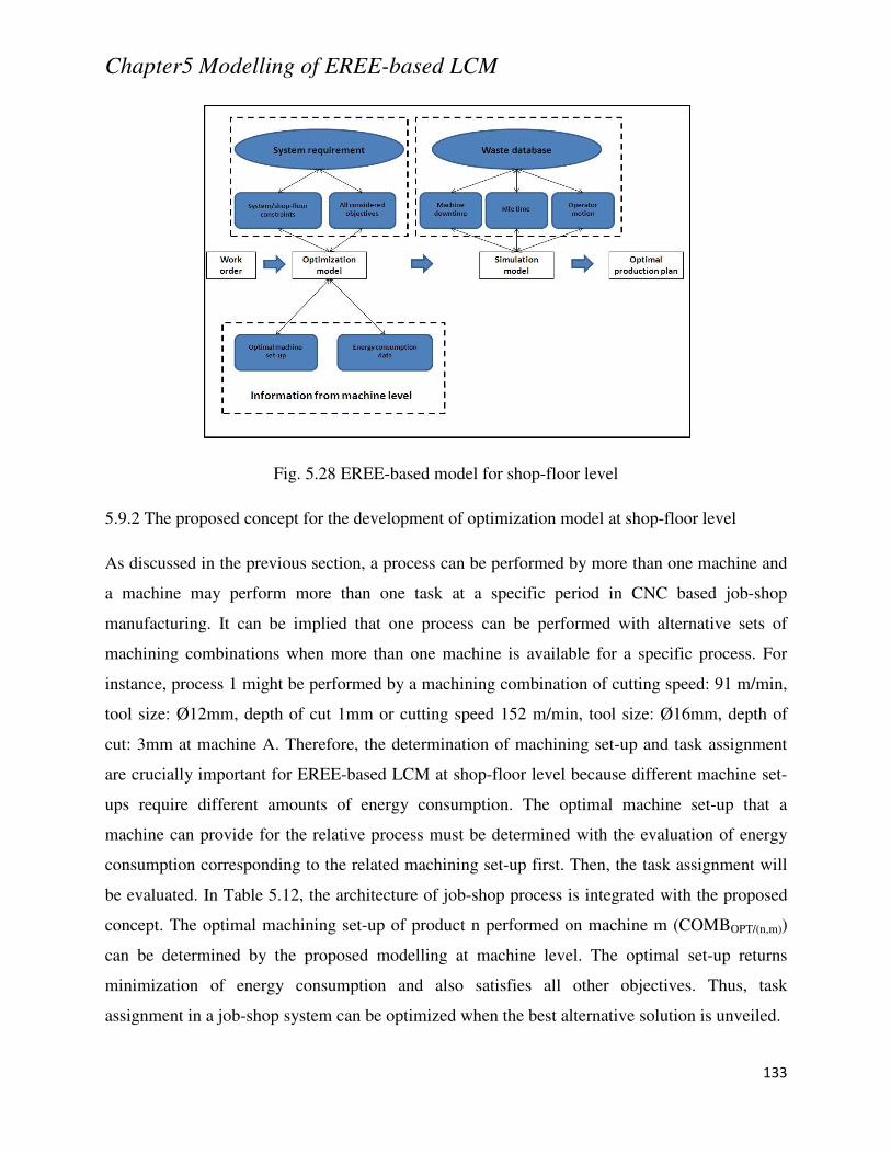
Chapter5 Modelling of EREE-based LCM
133
Fig. 5.28 EREE-based model for shop-floor level
5.9.2 The proposed concept for the development of optimization model at shop-floor level
As discussed in the previous section, a process can be performed by more than one machine and
a machine may perform more than one task at a specific period in CNC based job-shop
manufacturing. It can be implied that one process can be performed with alternative sets of
machining combinations when more than one machine is available for a specific process. For
instance, process 1 might be performed by a machining combination of cutting speed: 91 m/min,
tool size: Ø12mm, depth of cut 1mm or cutting speed 152 m/min, tool size: Ø16mm, depth of
cut: 3mm at machine A. Therefore, the determination of machining set-up and task assignment
are crucially important for EREE-based LCM at shop-floor level because different machine set-
ups require different amounts of energy consumption. The optimal machine set-up that a
machine can provide for the relative process must be determined with the evaluation of energy
consumption corresponding to the related machining set-up first. Then, the task assignment will
be evaluated. In Table 5.12, the architecture of job-shop process is integrated with the proposed
concept. The optimal machining set-up of product n performed on machine m (COMBOPT/(n,m))
can be determined by the proposed modelling at machine level. The optimal set-up returns
minimization of energy consumption and also satisfies all other objectives. Thus, task
assignment in a job-shop system can be optimized when the best alternative solution is unveiled.
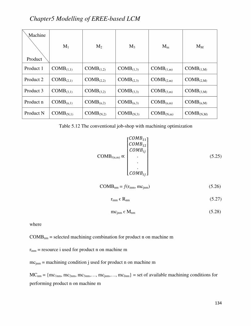
Chapter5 Modelling of EREE-based LCM
134
Machine
Product
M1 M2 M3 Mm MM
Product 1 COMB(1,1) COMB(1,2) COMB(1,3) COMB(1,m) COMB(1,M)
Product 2 COMB(2,1) COMB(2,2) COMB(2,3) COMB(2,m) COMB(2,M)
Product 3 COMB(3,1) COMB(3,2) COMB(3,3) COMB(3,m) COMB(3,M)
Product n COMB(n,1) COMB(n,2) COMB(n,3) COMB(n,m) COMB(n,M)
Product N COMB(N,1) COMB(N,2) COMB(N,3) COMB(N,m) COMB(N,M)
Table 5.12 The conventional job-shop with machining optimization
COMB/(n,m) C ;<<<<<=>eD>eD>eD"l...>eD~ @A
AAAAB (5.25)
COMBnm = ƒ(rinm, mcjnm) (5.26)
rinm є Rnm (5.27)
mcjnm є Mnm (5.28)
where
COMBnm = selected machining combination for product n on machine m
rinm = resource i used for product n on machine m
mcjnm = machining condition j used for product n on machine m
MCnm = mc1nm, mc2nm, mc3nm,…, mcjnm,…, mcJnm = set of available machining conditions for
performing product n on machine m
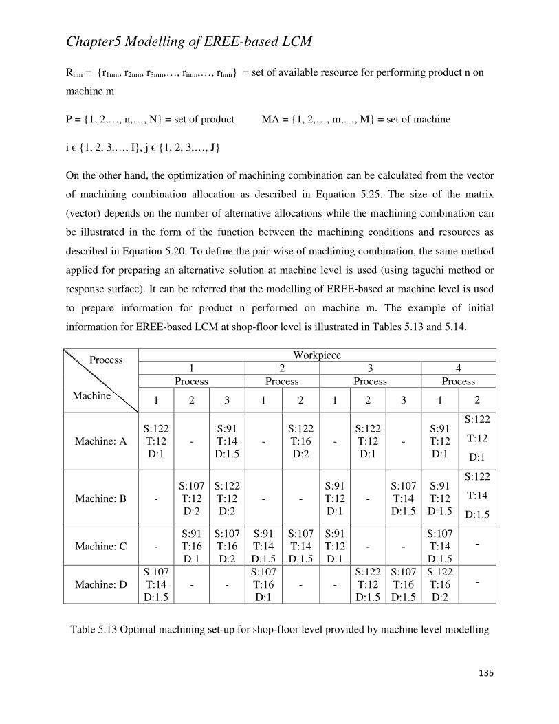
Chapter5 Modelling of EREE-based LCM
135
Rnm = r1nm, r2nm, r3nm,…, rinm,…, rInm = set of available resource for performing product n on
machine m
P = 1, 2,…, n,…, N = set of product MA = 1, 2,…, m,…, M = set of machine
i є 1, 2, 3,…, I, j є 1, 2, 3,…, J
On the other hand, the optimization of machining combination can be calculated from the vector
of machining combination allocation as described in Equation 5.25. The size of the matrix
(vector) depends on the number of alternative allocations while the machining combination can
be illustrated in the form of the function between the machining conditions and resources as
described in Equation 5.20. To define the pair-wise of machining combination, the same method
applied for preparing an alternative solution at machine level is used (using taguchi method or
response surface). It can be referred that the modelling of EREE-based at machine level is used
to prepare information for product n performed on machine m. The example of initial
information for EREE-based LCM at shop-floor level is illustrated in Tables 5.13 and 5.14.
Workpiece 1 2 3 4
Process Process Process Process
1 2 3 1 2 1 2 3 1 2
Machine: A S:122 T:12 D:1
- S:91 T:14 D:1.5
- S:122 T:16 D:2
- S:122 T:12 D:1
- S:91 T:12 D:1
S:122
T:12
D:1
Machine: B - S:107 T:12 D:2
S:122 T:12 D:2
- - S:91 T:12 D:1
- S:107 T:14 D:1.5
S:91 T:12 D:1.5
S:122
T:14
D:1.5
Machine: C - S:91 T:16 D:1
S:107 T:16 D:2
S:91 T:14 D:1.5
S:107 T:14 D:1.5
S:91 T:12 D:1
- - S:107 T:14 D:1.5
-
Machine: D S:107 T:14 D:1.5
- - S:107 T:16 D:1
- - S:122 T:12 D:1.5
S:107 T:16 D:1.5
S:122 T:16 D:2
-
Table 5.13 Optimal machining set-up for shop-floor level provided by machine level modelling
Machine
Process
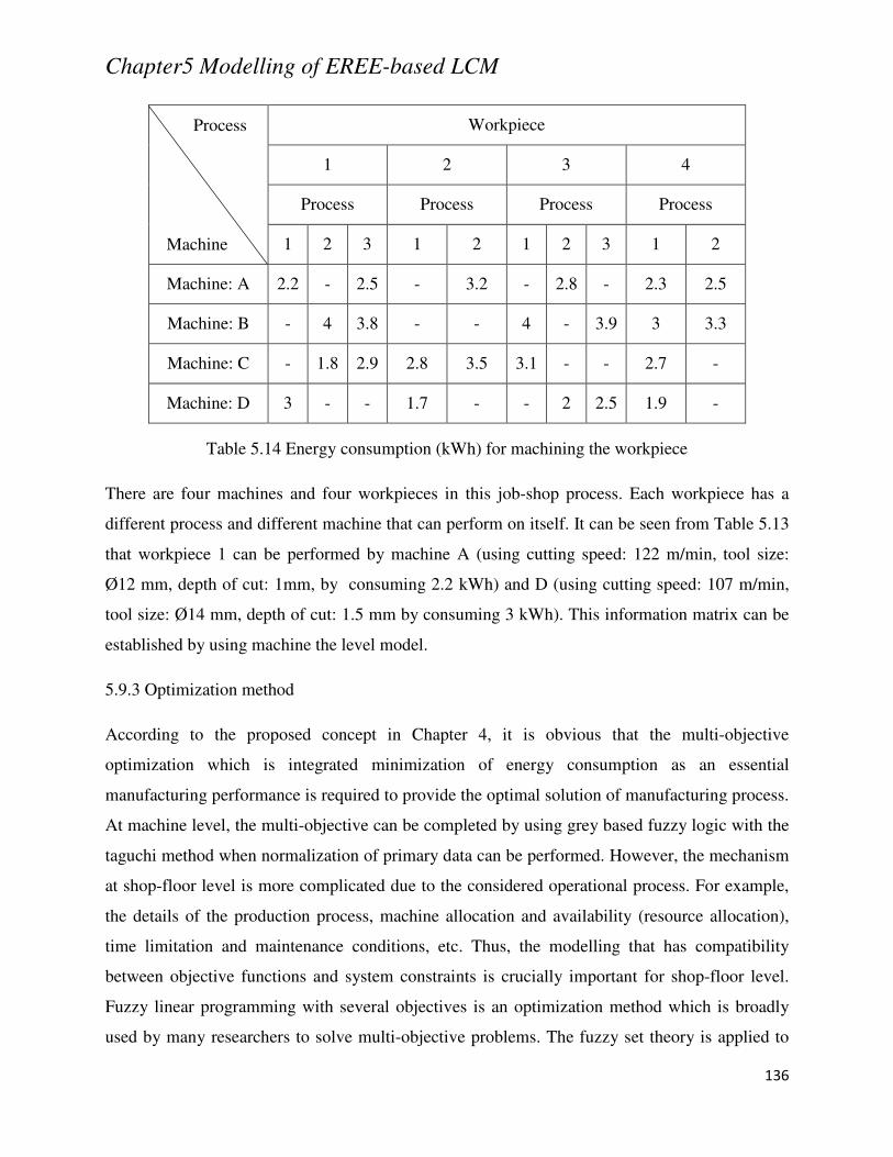
Chapter5 Modelling of EREE-based LCM
136
Workpiece
1 2 3 4
Process Process Process Process
1 2 3 1 2 1 2 3 1 2
Machine: A 2.2 - 2.5 - 3.2 - 2.8 - 2.3 2.5
Machine: B - 4 3.8 - - 4 - 3.9 3 3.3
Machine: C - 1.8 2.9 2.8 3.5 3.1 - - 2.7 -
Machine: D 3 - - 1.7 - - 2 2.5 1.9 -
Table 5.14 Energy consumption (kWh) for machining the workpiece
There are four machines and four workpieces in this job-shop process. Each workpiece has a
different process and different machine that can perform on itself. It can be seen from Table 5.13
that workpiece 1 can be performed by machine A (using cutting speed: 122 m/min, tool size:
Ø12 mm, depth of cut: 1mm, by consuming 2.2 kWh) and D (using cutting speed: 107 m/min,
tool size: Ø14 mm, depth of cut: 1.5 mm by consuming 3 kWh). This information matrix can be
established by using machine the level model.
5.9.3 Optimization method
According to the proposed concept in Chapter 4, it is obvious that the multi-objective
optimization which is integrated minimization of energy consumption as an essential
manufacturing performance is required to provide the optimal solution of manufacturing process.
At machine level, the multi-objective can be completed by using grey based fuzzy logic with the
taguchi method when normalization of primary data can be performed. However, the mechanism
at shop-floor level is more complicated due to the considered operational process. For example,
the details of the production process, machine allocation and availability (resource allocation),
time limitation and maintenance conditions, etc. Thus, the modelling that has compatibility
between objective functions and system constraints is crucially important for shop-floor level.
Fuzzy linear programming with several objectives is an optimization method which is broadly
used by many researchers to solve multi-objective problems. The fuzzy set theory is applied to
Machine
Process
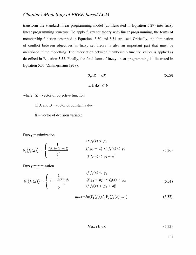
Chapter5 Modelling of EREE-based LCM
137
transform the standard linear programming model (as illustrated in Equation 5.29) into fuzzy
linear programming structure. To apply fuzzy set theory with linear programming, the terms of
membership function described in Equations 5.30 and 5.31 are used. Critically, the elimination
of conflict between objectives in fuzzy set theory is also an important part that must be
mentioned in the modelling. The intersection between membership function values is applied as
described in Equation 5.32. Finally, the final form of fuzzy linear programming is illustrated in
Equation 5.33 (Zimmermann 1978).
>1 (5.29)
L. . 1
where: Z = vector of objective function
C, A and B = vector of constant value
X = vector of decision variable
Fuzzy maximization
1 .fk k** 0 P (5.30)
Fuzzy minimization
1 1 9 .|fk |*|| 0 P (5.31)
, ,… . (5.32)
e e (5.33)
9
9
7 7
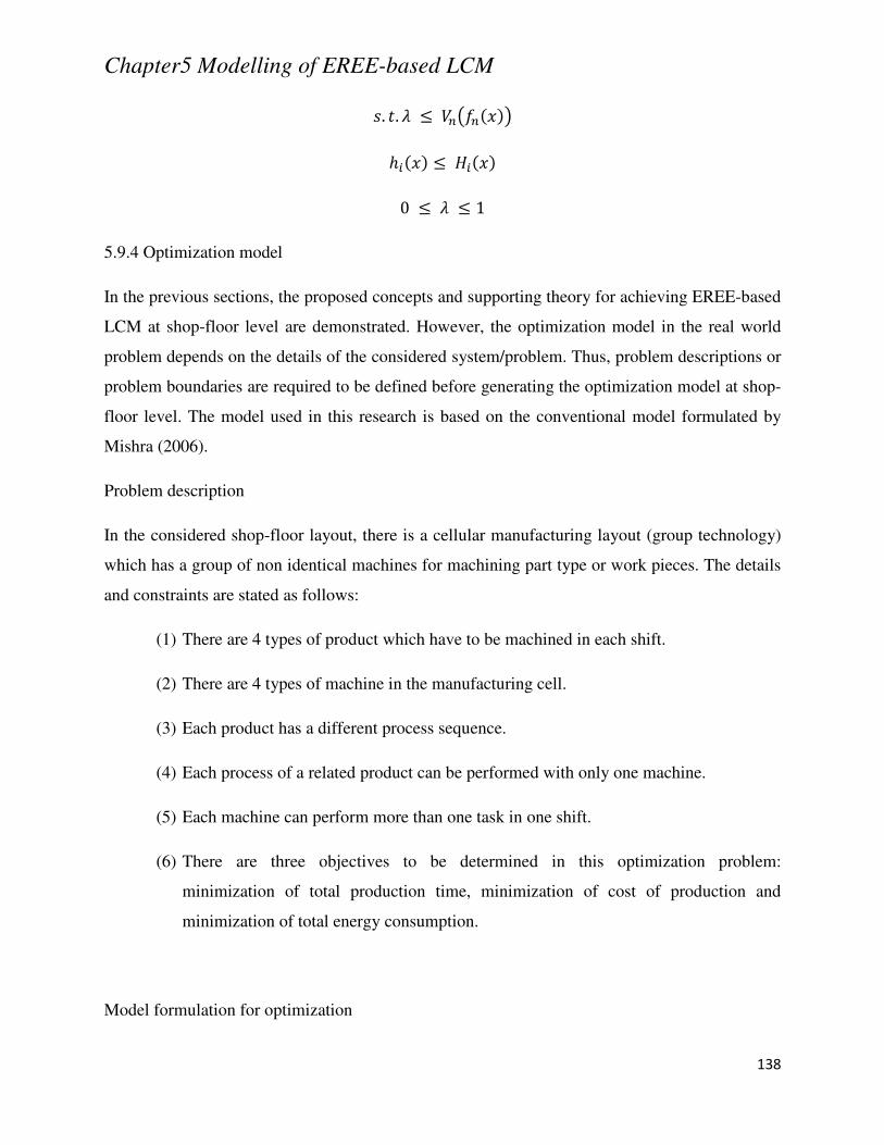
Chapter5 Modelling of EREE-based LCM
138
L. . ,, " " 0 1
5.9.4 Optimization model
In the previous sections, the proposed concepts and supporting theory for achieving EREE-based
LCM at shop-floor level are demonstrated. However, the optimization model in the real world
problem depends on the details of the considered system/problem. Thus, problem descriptions or
problem boundaries are required to be defined before generating the optimization model at shop-
floor level. The model used in this research is based on the conventional model formulated by
Mishra (2006).
Problem description
In the considered shop-floor layout, there is a cellular manufacturing layout (group technology)
which has a group of non identical machines for machining part type or work pieces. The details
and constraints are stated as follows:
(1) There are 4 types of product which have to be machined in each shift.
(2) There are 4 types of machine in the manufacturing cell.
(3) Each product has a different process sequence.
(4) Each process of a related product can be performed with only one machine.
(5) Each machine can perform more than one task in one shift.
(6) There are three objectives to be determined in this optimization problem:
minimization of total production time, minimization of cost of production and
minimization of total energy consumption.
Model formulation for optimization
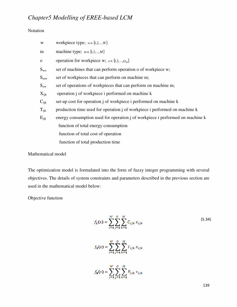
Chapter5 Modelling of EREE
Notation
w workpiece type; w
m machine type; m ∈
o operation for workpiece w;
Swo set of machines that can perform operation o of workpiece w;
Smw set of workpieces
Sow set of operations of workpiece
Xijk operation j of workpiece i perform
Cijk set-up cost for operation j of workpiece i perform
Tijk production time used
Eijk energy consumption used
function of total energy consumption
function of total cost of operation
function of total production time
Mathematical model
The optimization model is formulated into the form of fuzzy integer programming with several
objectives. The details of system constraints and parameters described in the previous section are
used in the mathematical model below:
Objective function
Chapter5 Modelling of EREE-based LCM
Ww ,...,2,1∈
M,...,2,1∈
operation for workpiece w; Owo ,...,2,1∈
that can perform operation o of workpiece w;
that can perform on machine m;
of workpieces that can perform on machine m;
of workpiece i performed on machine k
up cost for operation j of workpiece i performed on machine k
production time used for operation j of workpiece i performed on machine k
energy consumption used for operation j of workpiece i performed
function of total energy consumption
function of total cost of operation
function of total production time
model is formulated into the form of fuzzy integer programming with several
objectives. The details of system constraints and parameters described in the previous section are
used in the mathematical model below:
139
on machine k
on machine k
ed on machine k
model is formulated into the form of fuzzy integer programming with several
objectives. The details of system constraints and parameters described in the previous section are
(5.34)
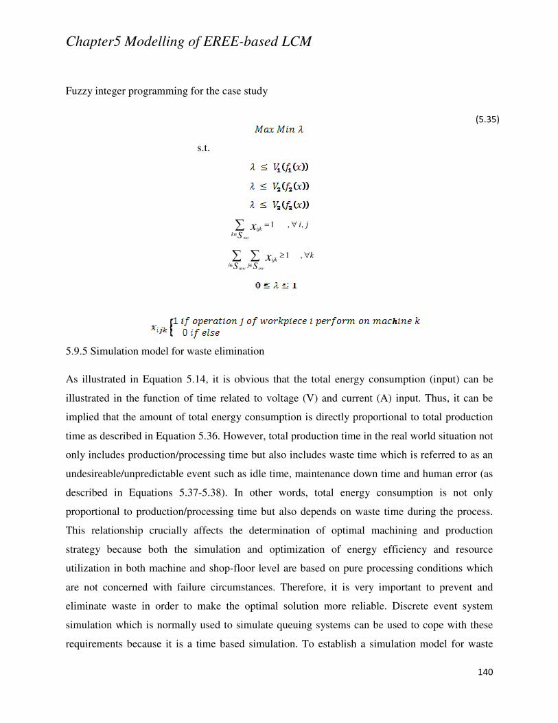
Chapter5 Modelling of EREE
Fuzzy integer programming for the case study
s.t.
5.9.5 Simulation model for waste elimination
As illustrated in Equation 5.14, it is obvious that the total ene
illustrated in the function of time related to voltage (V) and current (A) input. Thus, it can be
implied that the amount of total energy consumption is directly proportion
time as described in Equation 5.36
only includes production/processing time but also includes waste time which is referred to
undesireable/unpredictable event such as idle time, maintenance down time and human er
described in Equations 5.37-5.38
proportional to production/processing time but also depends on waste time during
This relationship crucially affect
strategy because both the simulation and optimization of energy efficiency and resource
utilization in both machine and shop
are not concerned with failure circumstances. Therefo
eliminate waste in order to make
simulation which is normally used to simulate queuing system
requirements because it is a tim
Chapter5 Modelling of EREE-based LCM
Fuzzy integer programming for the case study
s.t.
∑∈
∀=
S wok
ijkjix ,,1
∑ ∑∈ ∈
∀≥
S Smw owi j
ijkkx ,1
Simulation model for waste elimination
, it is obvious that the total energy consumption (input) can be
illustrated in the function of time related to voltage (V) and current (A) input. Thus, it can be
that the amount of total energy consumption is directly proportional to total production
5.36. However, total production time in the real world situation not
only includes production/processing time but also includes waste time which is referred to
undesireable/unpredictable event such as idle time, maintenance down time and human er
5.38). In other words, total energy consumption
proportional to production/processing time but also depends on waste time during
This relationship crucially affects the determination of optimal machining and production
simulation and optimization of energy efficiency and resource
utilization in both machine and shop-floor level are based on pure processing conditions which
with failure circumstances. Therefore, it is very important to prevent and
eliminate waste in order to make the optimal solution more reliable. Discrete event system
simulation which is normally used to simulate queuing systems can be used to cope with these
requirements because it is a time based simulation. To establish a simulation model for waste
140
rgy consumption (input) can be
illustrated in the function of time related to voltage (V) and current (A) input. Thus, it can be
to total production
. However, total production time in the real world situation not
only includes production/processing time but also includes waste time which is referred to as an
undesireable/unpredictable event such as idle time, maintenance down time and human error (as
). In other words, total energy consumption is not only
proportional to production/processing time but also depends on waste time during the process.
ning and production
simulation and optimization of energy efficiency and resource
floor level are based on pure processing conditions which
re, it is very important to prevent and
optimal solution more reliable. Discrete event system
can be used to cope with these
simulation model for waste
(5.35)
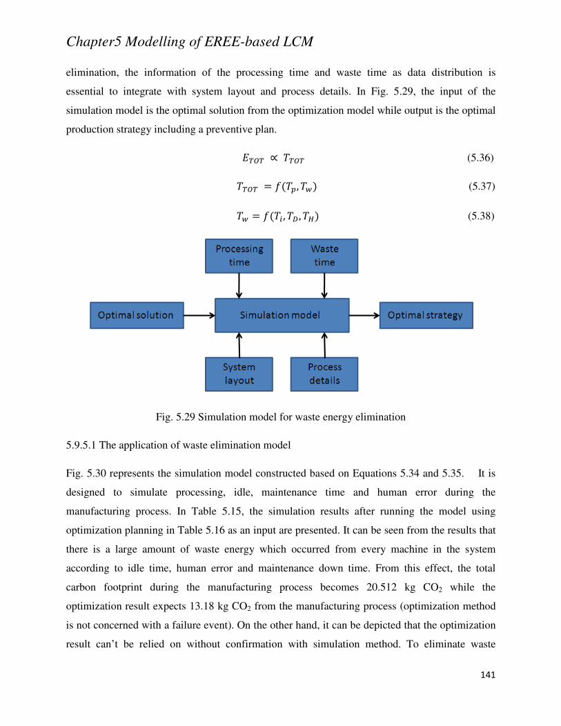
Chapter5 Modelling of EREE-based LCM
141
elimination, the information of the processing time and waste time as data distribution is
essential to integrate with system layout and process details. In Fig. 5.29, the input of the
simulation model is the optimal solution from the optimization model while output is the optimal
production strategy including a preventive plan.
\z\ C \z\ (5.36)
\z\ -, (5.37)
", , (5.38)
Fig. 5.29 Simulation model for waste energy elimination
5.9.5.1 The application of waste elimination model
Fig. 5.30 represents the simulation model constructed based on Equations 5.34 and 5.35. It is
designed to simulate processing, idle, maintenance time and human error during the
manufacturing process. In Table 5.15, the simulation results after running the model using
optimization planning in Table 5.16 as an input are presented. It can be seen from the results that
there is a large amount of waste energy which occurred from every machine in the system
according to idle time, human error and maintenance down time. From this effect, the total
carbon footprint during the manufacturing process becomes 20.512 kg CO2 while the
optimization result expects 13.18 kg CO2 from the manufacturing process (optimization method
is not concerned with a failure event). On the other hand, it can be depicted that the optimization
result can’t be relied on without confirmation with simulation method. To eliminate waste
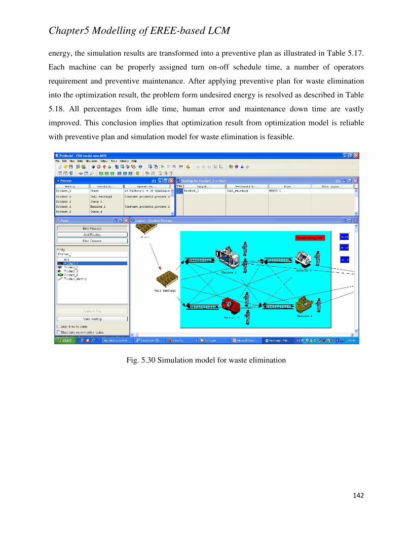
Chapter5 Modelling of EREE-based LCM
142
energy, the simulation results are transformed into a preventive plan as illustrated in Table 5.17.
Each machine can be properly assigned turn on-off schedule time, a number of operators
requirement and preventive maintenance. After applying preventive plan for waste elimination
into the optimization result, the problem form undesired energy is resolved as described in Table
5.18. All percentages from idle time, human error and maintenance down time are vastly
improved. This conclusion implies that optimization result from optimization model is reliable
with preventive plan and simulation model for waste elimination is feasible.
Fig. 5.30 Simulation model for waste elimination
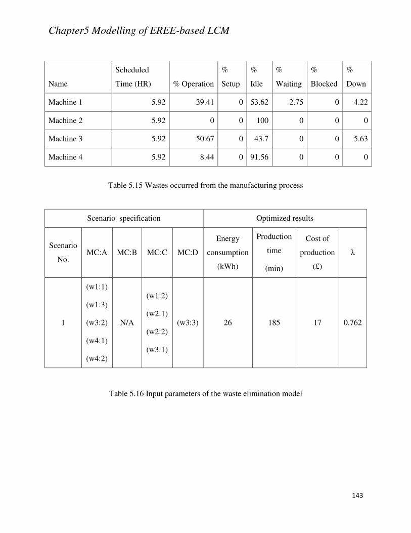
Chapter5 Modelling of EREE-based LCM
143
Table 5.15 Wastes occurred from the manufacturing process
Table 5.16 Input parameters of the waste elimination model
Name
Scheduled
Time (HR) % Operation
%
Setup
%
Idle
%
Waiting
%
Blocked
%
Down
Machine 1 5.92 39.41 0 53.62 2.75 0 4.22
Machine 2 5.92 0 0 100 0 0 0
Machine 3 5.92 50.67 0 43.7 0 0 5.63
Machine 4 5.92 8.44 0 91.56 0 0 0
Scenario specification Optimized results
Scenario
No. MC:A MC:B MC:C MC:D
Energy
consumption
(kWh)
Production
time
(min)
Cost of
production
(£)
λ
1
(w1:1)
(w1:3)
(w3:2)
(w4:1)
(w4:2)
N/A
(w1:2)
(w2:1)
(w2:2)
(w3:1)
(w3:3) 26 185 17 0.762
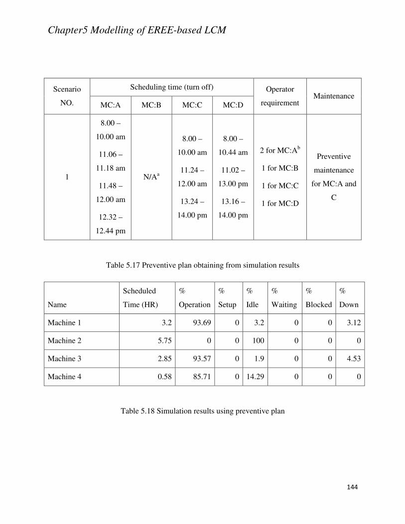
Chapter5 Modelling of EREE-based LCM
144
Table 5.17 Preventive plan obtaining from simulation results
Table 5.18 Simulation results using preventive plan
Scenario
NO.
Scheduling time (turn off) Operator
requirement Maintenance
MC:A MC:B MC:C MC:D
1
8.00 –
10.00 am
11.06 –
11.18 am
11.48 –
12.00 am
12.32 –
12.44 pm
N/Aa
8.00 –
10.00 am
11.24 –
12.00 am
13.24 –
14.00 pm
8.00 –
10.44 am
11.02 –
13.00 pm
13.16 –
14.00 pm
2 for MC:Ab
1 for MC:B
1 for MC:C
1 for MC:D
Preventive
maintenance
for MC:A and
C
Name
Scheduled
Time (HR)
%
Operation
%
Setup
%
Idle
%
Waiting
%
Blocked
%
Down
Machine 1 3.2 93.69 0 3.2 0 0 3.12
Machine 2 5.75 0 0 100 0 0 0
Machine 3 2.85 93.57 0 1.9 0 0 4.53
Machine 4 0.58 85.71 0 14.29 0 0 0
Chapter5 Modelling of EREE-based LCM
145
5.10 Summary
Fuzzy logic using mamdani and sugeno type techniques is used to develop EREE-based LCM
modelling at the machine level. The architecture of the evaluation mechanism is constructed
based on a cutting force model and experimental data. The experiment (cutting trial) has been
made on aluminum material with a CNC milling machine. A MATLAB-based simulation system
has been developed to facilitate and perform energy/resource simulation and optimization. From
the simulation results, the following conclusions can be drawn:
(1) The simulation results from the modelling have the same trend with experimental data. It
is also more reliable compared to results from a MATLAB-based response surface
methodology.
(2) The result from the developed model provides the optimization of energy efficiency and
resource utilization with the compromise between all other objectives.
This chapter has also presented a development of EREE-based LCM at shop-floor level. The
developed systematic modelling includes two sub-models i.e. an optimization model cooperating
with a machine level model and waste elimination model. The optimization model is formulated
based on the information of the process sequence of the considered system. The input for this
model uses a proposed matrix with optimal results from the machine level model while the
optimization process uses fuzzy linear programming with several objectives. The output from
this model provides an optimal production plan together with an optimal machining set-up in
order to minimize the total carbon footprint and also satisfy all other objectives. For the waste
elimination model, it is designed to eliminate waste energy during manufacturing processes by
using discrete event system simulation theory to simulate failure events. ProModel software is
used to establish the model related to the mathematical formulation used for the optimization
model. The output from this model is a preventive plan used together with optimal production to
eliminate waste energy. As part of the framework proposed for developing EREE-based LCM,
the evaluation and validation of the developed models for machine and shop-floor level will be
carried out in the next chapter.
Chapter6 Application case studies
146
Chapter 6 Application case studies
6.1 Introduction
This chapter presents the evaluation of the framework proposed for developing EREE-based
LCM through two case studies. Since the framework includes a number of aspects, only partial
evaluations are considered in this chapter.
The first case study is concerned with EREE-based LCM at machine level. The experimental
data obtained from cutting trials is used to formulate learning rules. The prediction results from
the proposed model are, then, compared with the conventional statistical methods.
The second case study is related to EREE-based LCM at shop-floor level. The numerical
example is demonstrated with initial information (input data). The combination of an
optimization model and a simulation model represents the integration of energy efficiency,
resource utilization and waste minimization throughout the minimization of the carbon footprint.
6.2 EREE-based LCM case study one
In this case study, the investigation on energy consumption of the conventional CNC milling
machine using aluminum as a material, is used. The objective of this case study is to determine
the optimal machining set-up that can satisfy energy efficiency and even reduce the total carbon
footprint.
6.2.1 Experimental set-up
To perform these experiments, the 5 axis CNC milling machine with 10 kW motor speeds
corresponding with 6000 rpm maximum spindle speed and 35 m/min maximum feed rate is used
to proceed all cutting trials. The flexible AC power quality tester (PRIMUS PC-02) is connected
to the main power supply using the three phase electrical system of the machine in order to
measure the total energy consumption (kWh) per cutting trial. To connect the power quality
tester with the CNC machine, the first voltage test lead is connected to the phase no.1 and the
second voltage test lead is connected to the phase no.3. The flexible loop is connected to the
phase no.2. In Fig. 6.1, the connection of the measurement device and the 3-phase main power
supply is illustrated. The full experimental set-up is depicted in Fig. 6.2. The measurement
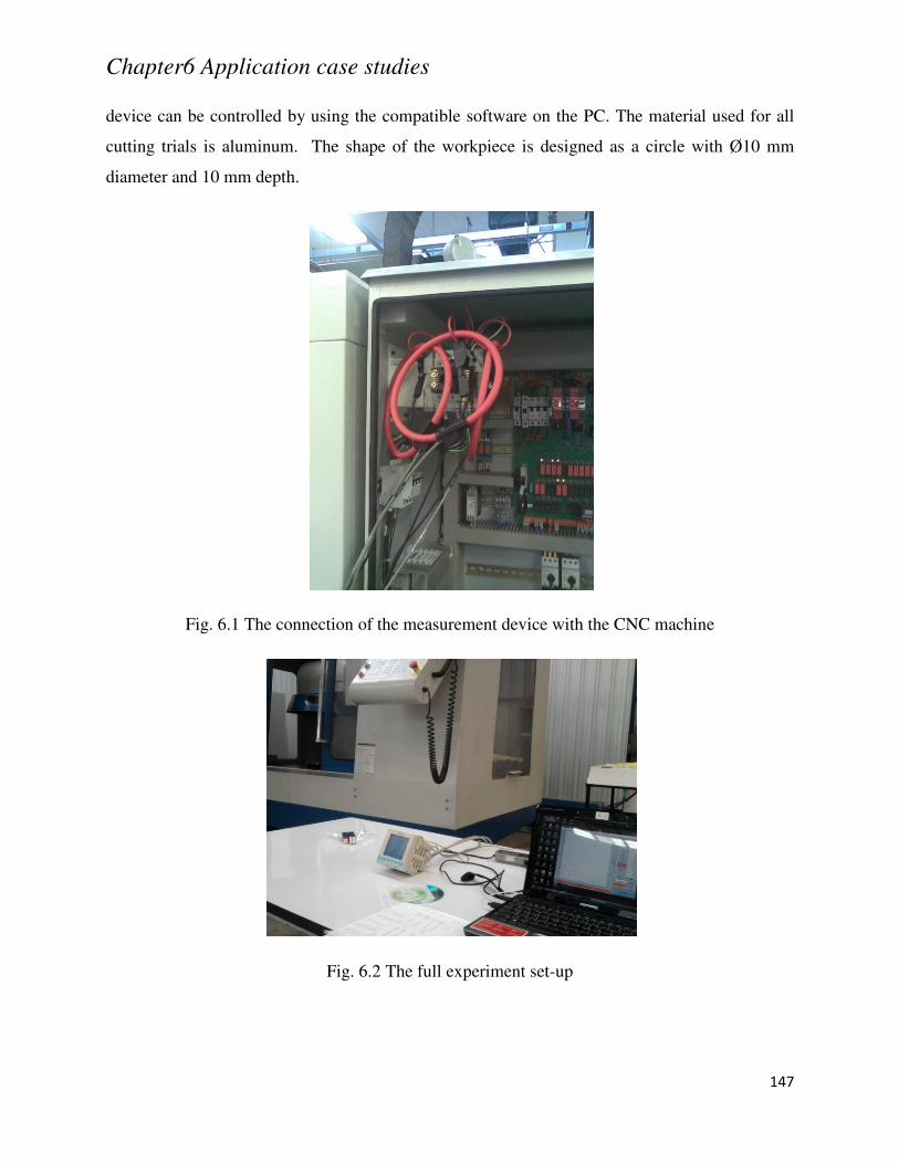
Chapter6 Application case studies
147
device can be controlled by using the compatible software on the PC. The material used for all
cutting trials is aluminum. The shape of the workpiece is designed as a circle with Ø10 mm
diameter and 10 mm depth.
Fig. 6.1 The connection of the measurement device with the CNC machine
Fig. 6.2 The full experiment set-up
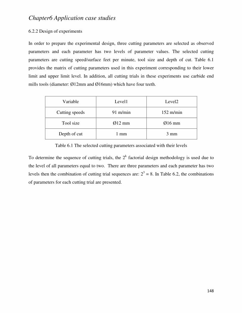
Chapter6 Application case studies
148
6.2.2 Design of experiments
In order to prepare the experimental design, three cutting parameters are selected as observed
parameters and each parameter has two levels of parameter values. The selected cutting
parameters are cutting speed/surface feet per minute, tool size and depth of cut. Table 6.1
provides the matrix of cutting parameters used in this experiment corresponding to their lower
limit and upper limit level. In addition, all cutting trials in these experiments use carbide end
mills tools (diameter: Ø12mm and Ø16mm) which have four teeth.
Table 6.1 The selected cutting parameters associated with their levels
To determine the sequence of cutting trials, the 2k factorial design methodology is used due to
the level of all parameters equal to two. There are three parameters and each parameter has two
levels then the combination of cutting trial sequences are: 23 = 8. In Table 6.2, the combinations
of parameters for each cutting trial are presented.
Variable Level1 Level2
Cutting speeds 91 m/min 152 m/min
Tool size Ø12 mm Ø16 mm
Depth of cut 1 mm 3 mm
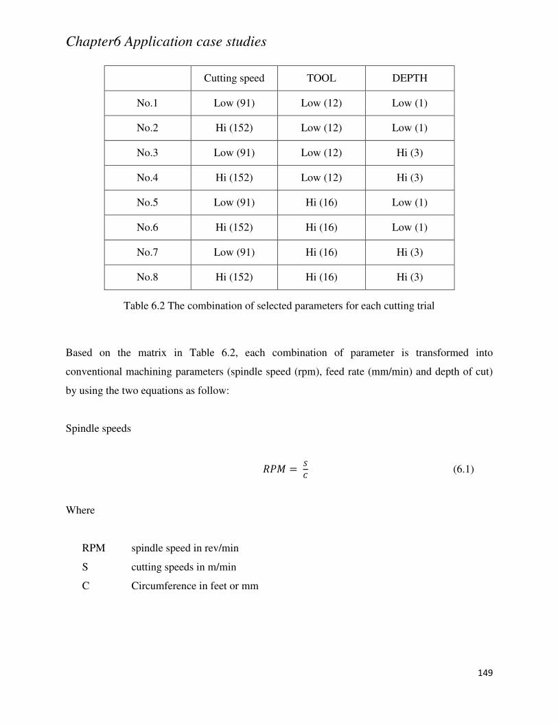
Chapter6 Application case studies
149
Cutting speed TOOL DEPTH
No.1 Low (91) Low (12) Low (1)
No.2 Hi (152) Low (12) Low (1)
No.3 Low (91) Low (12) Hi (3)
No.4 Hi (152) Low (12) Hi (3)
No.5 Low (91) Hi (16) Low (1)
No.6 Hi (152) Hi (16) Low (1)
No.7 Low (91) Hi (16) Hi (3)
No.8 Hi (152) Hi (16) Hi (3)
Table 6.2 The combination of selected parameters for each cutting trial
Based on the matrix in Table 6.2, each combination of parameter is transformed into
conventional machining parameters (spindle speed (rpm), feed rate (mm/min) and depth of cut)
by using the two equations as follow:
Spindle speeds
e (6.1)
Where
RPM spindle speed in rev/min
S cutting speeds in m/min
C Circumference in feet or mm
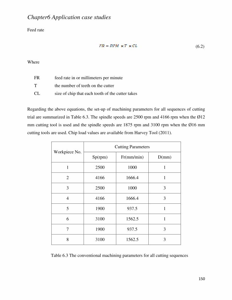
Chapter6 Application case studies
150
Feed rate
(6.2)
Where
FR feed rate in or millimeters per minute
T the number of teeth on the cutter
CL size of chip that each tooth of the cutter takes
Regarding the above equations, the set-up of machining parameters for all sequences of cutting
trial are summarized in Table 6.3. The spindle speeds are 2500 rpm and 4166 rpm when the Ø12
mm cutting tool is used and the spindle speeds are 1875 rpm and 3100 rpm when the Ø16 mm
cutting tools are used. Chip load values are available from Harvey Tool (2011).
Workpiece No. Cutting Parameters
Sp(rpm) Fr(mm/min) D(mm)
1 2500 1000 1
2 4166 1666.4 1
3 2500 1000 3
4 4166 1666.4 3
5 1900 937.5 1
6 3100 1562.5 1
7 1900 937.5 3
8 3100 1562.5 3
Table 6.3 The conventional machining parameters for all cutting sequences
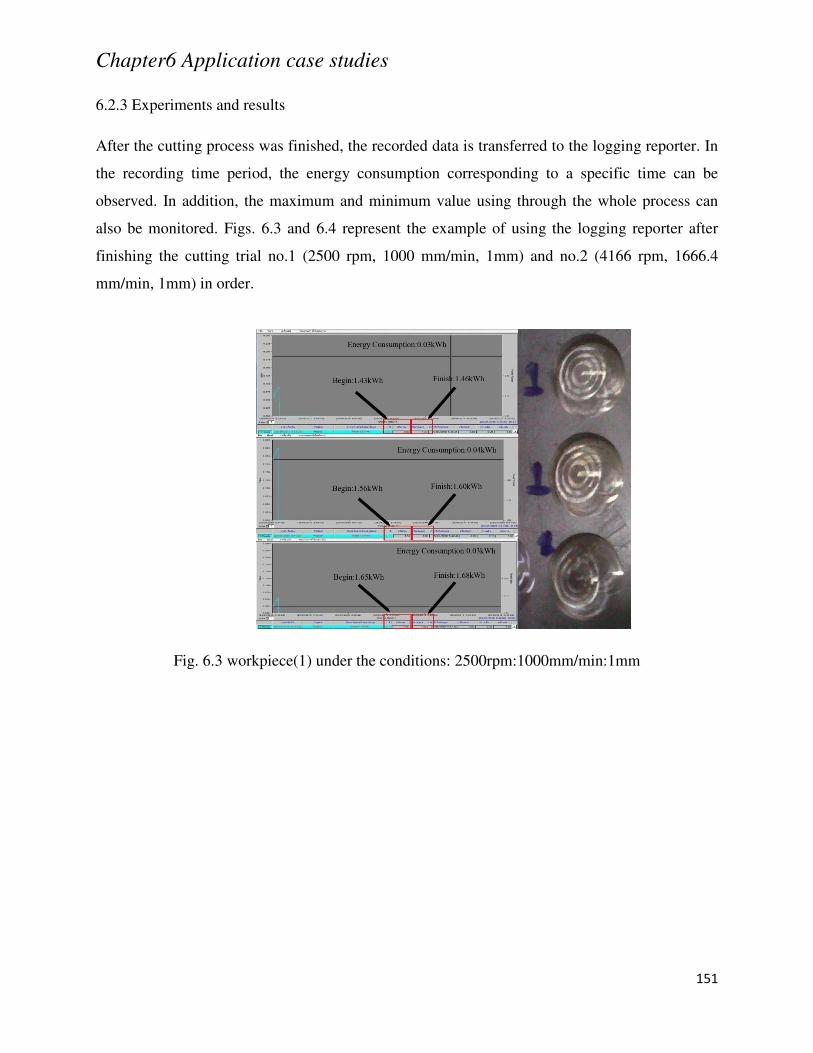
Chapter6 Application case studies
151
6.2.3 Experiments and results
After the cutting process was finished, the recorded data is transferred to the logging reporter. In
the recording time period, the energy consumption corresponding to a specific time can be
observed. In addition, the maximum and minimum value using through the whole process can
also be monitored. Figs. 6.3 and 6.4 represent the example of using the logging reporter after
finishing the cutting trial no.1 (2500 rpm, 1000 mm/min, 1mm) and no.2 (4166 rpm, 1666.4
mm/min, 1mm) in order.
Fig. 6.3 workpiece(1) under the conditions: 2500rpm:1000mm/min:1mm
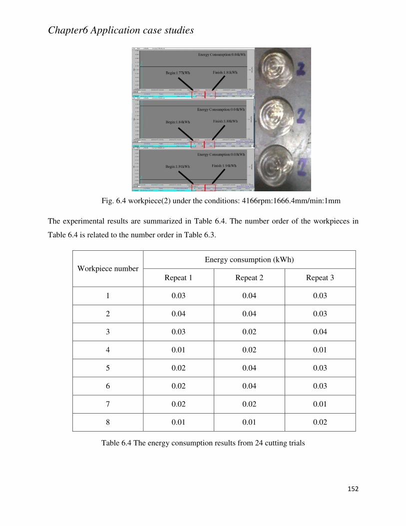
Chapter6 Application case studies
152
Fig. 6.4 workpiece(2) under the conditions: 4166rpm:1666.4mm/min:1mm
The experimental results are summarized in Table 6.4. The number order of the workpieces in
Table 6.4 is related to the number order in Table 6.3.
Workpiece number Energy consumption (kWh)
Repeat 1 Repeat 2 Repeat 3
1 0.03 0.04 0.03
2 0.04 0.04 0.03
3 0.03 0.02 0.04
4 0.01 0.02 0.01
5 0.02 0.04 0.03
6 0.02 0.04 0.03
7 0.02 0.02 0.01
8 0.01 0.01 0.02
Table 6.4 The energy consumption results from 24 cutting trials
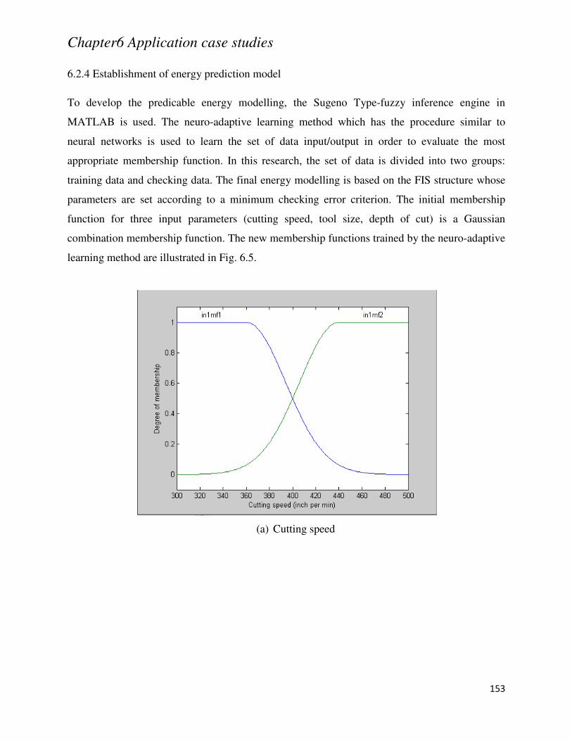
Chapter6 Application case studies
153
6.2.4 Establishment of energy prediction model
To develop the predicable energy modelling, the Sugeno Type-fuzzy inference engine in
MATLAB is used. The neuro-adaptive learning method which has the procedure similar to
neural networks is used to learn the set of data input/output in order to evaluate the most
appropriate membership function. In this research, the set of data is divided into two groups:
training data and checking data. The final energy modelling is based on the FIS structure whose
parameters are set according to a minimum checking error criterion. The initial membership
function for three input parameters (cutting speed, tool size, depth of cut) is a Gaussian
combination membership function. The new membership functions trained by the neuro-adaptive
learning method are illustrated in Fig. 6.5.
(a) Cutting speed
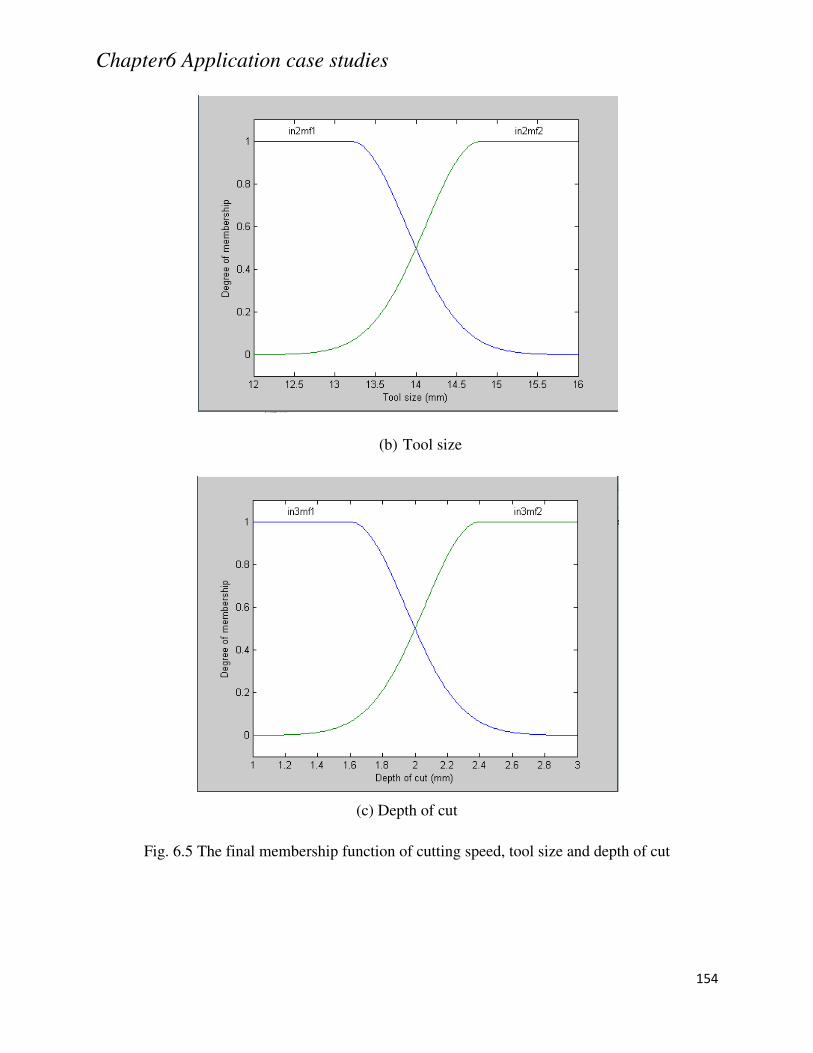
Chapter6 Application case studies
154
(b) Tool size
(c) Depth of cut
Fig. 6.5 The final membership function of cutting speed, tool size and depth of cut
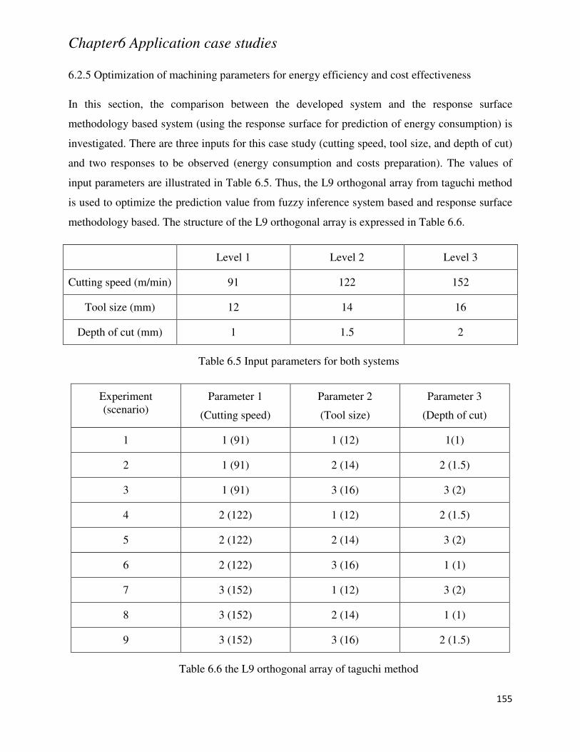
Chapter6 Application case studies
155
6.2.5 Optimization of machining parameters for energy efficiency and cost effectiveness
In this section, the comparison between the developed system and the response surface
methodology based system (using the response surface for prediction of energy consumption) is
investigated. There are three inputs for this case study (cutting speed, tool size, and depth of cut)
and two responses to be observed (energy consumption and costs preparation). The values of
input parameters are illustrated in Table 6.5. Thus, the L9 orthogonal array from taguchi method
is used to optimize the prediction value from fuzzy inference system based and response surface
methodology based. The structure of the L9 orthogonal array is expressed in Table 6.6.
Level 1 Level 2 Level 3
Cutting speed (m/min) 91 122 152
Tool size (mm) 12 14 16
Depth of cut (mm) 1 1.5 2
Table 6.5 Input parameters for both systems
Experiment (scenario)
Parameter 1
(Cutting speed)
Parameter 2
(Tool size)
Parameter 3
(Depth of cut)
1 1 (91) 1 (12) 1(1)
2 1 (91) 2 (14) 2 (1.5)
3 1 (91) 3 (16) 3 (2)
4 2 (122) 1 (12) 2 (1.5)
5 2 (122) 2 (14) 3 (2)
6 2 (122) 3 (16) 1 (1)
7 3 (152) 1 (12) 3 (2)
8 3 (152) 2 (14) 1 (1)
9 3 (152) 3 (16) 2 (1.5)
Table 6.6 the L9 orthogonal array of taguchi method
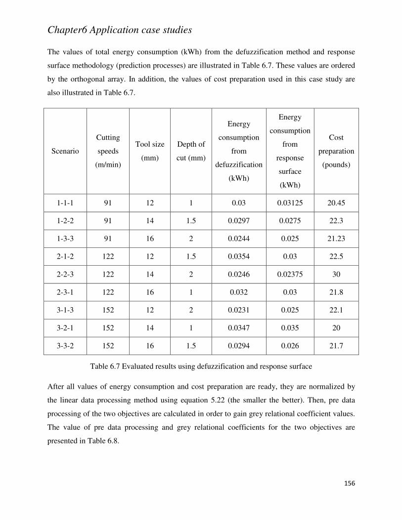
Chapter6 Application case studies
156
The values of total energy consumption (kWh) from the defuzzification method and response
surface methodology (prediction processes) are illustrated in Table 6.7. These values are ordered
by the orthogonal array. In addition, the values of cost preparation used in this case study are
also illustrated in Table 6.7.
Scenario
Cutting
speeds
(m/min)
Tool size
(mm)
Depth of
cut (mm)
Energy
consumption
from
defuzzification
(kWh)
Energy
consumption
from
response
surface
(kWh)
Cost
preparation
(pounds)
1-1-1 91 12 1 0.03 0.03125 20.45
1-2-2 91 14 1.5 0.0297 0.0275 22.3
1-3-3 91 16 2 0.0244 0.025 21.23
2-1-2 122 12 1.5 0.0354 0.03 22.5
2-2-3 122 14 2 0.0246 0.02375 30
2-3-1 122 16 1 0.032 0.03 21.8
3-1-3 152 12 2 0.0231 0.025 22.1
3-2-1 152 14 1 0.0347 0.035 20
3-3-2 152 16 1.5 0.0294 0.026 21.7
Table 6.7 Evaluated results using defuzzification and response surface
After all values of energy consumption and cost preparation are ready, they are normalized by
the linear data processing method using equation 5.22 (the smaller the better). Then, pre data
processing of the two objectives are calculated in order to gain grey relational coefficient values.
The value of pre data processing and grey relational coefficients for the two objectives are
presented in Table 6.8.
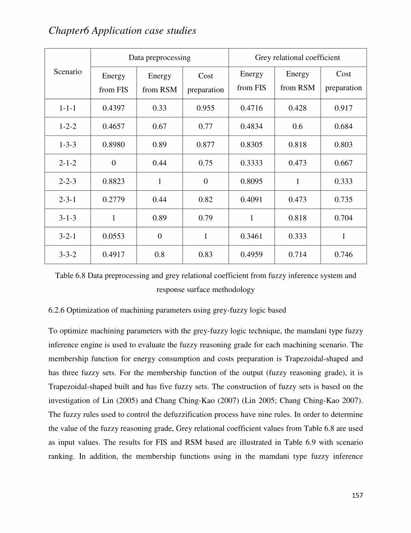
Chapter6 Application case studies
157
Scenario
Data preprocessing Grey relational coefficient
Energy
from FIS
Energy
from RSM
Cost
preparation
Energy
from FIS
Energy
from RSM
Cost
preparation
1-1-1 0.4397 0.33 0.955 0.4716 0.428 0.917
1-2-2 0.4657 0.67 0.77 0.4834 0.6 0.684
1-3-3 0.8980 0.89 0.877 0.8305 0.818 0.803
2-1-2 0 0.44 0.75 0.3333 0.473 0.667
2-2-3 0.8823 1 0 0.8095 1 0.333
2-3-1 0.2779 0.44 0.82 0.4091 0.473 0.735
3-1-3 1 0.89 0.79 1 0.818 0.704
3-2-1 0.0553 0 1 0.3461 0.333 1
3-3-2 0.4917 0.8 0.83 0.4959 0.714 0.746
Table 6.8 Data preprocessing and grey relational coefficient from fuzzy inference system and
response surface methodology
6.2.6 Optimization of machining parameters using grey-fuzzy logic based
To optimize machining parameters with the grey-fuzzy logic technique, the mamdani type fuzzy
inference engine is used to evaluate the fuzzy reasoning grade for each machining scenario. The
membership function for energy consumption and costs preparation is Trapezoidal-shaped and
has three fuzzy sets. For the membership function of the output (fuzzy reasoning grade), it is
Trapezoidal-shaped built and has five fuzzy sets. The construction of fuzzy sets is based on the
investigation of Lin (2005) and Chang Ching-Kao (2007) (Lin 2005; Chang Ching-Kao 2007).
The fuzzy rules used to control the defuzzification process have nine rules. In order to determine
the value of the fuzzy reasoning grade, Grey relational coefficient values from Table 6.8 are used
as input values. The results for FIS and RSM based are illustrated in Table 6.9 with scenario
ranking. In addition, the membership functions using in the mamdani type fuzzy inference
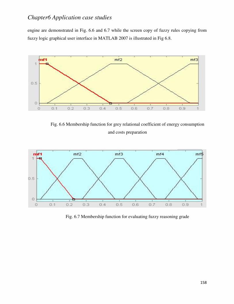
Chapter6 Application case studies
158
engine are demonstrated in Fig. 6.6 and 6.7 while the screen copy of fuzzy rules copying from
fuzzy logic graphical user interface in MATLAB 2007 is illustrated in Fig 6.8.
Fig. 6.6 Membership function for grey relational coefficient of energy consumption
and costs preparation
Fig. 6.7 Membership function for evaluating fuzzy reasoning grade
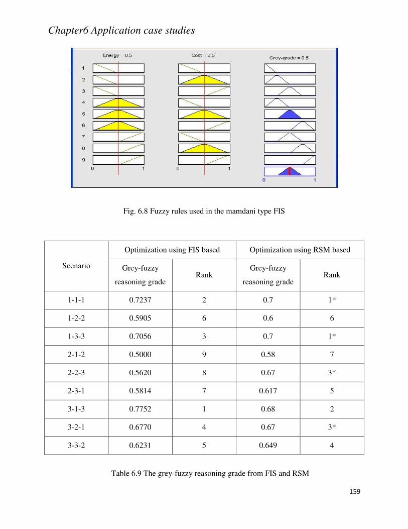
Chapter6 Application case studies
159
Fig. 6.8 Fuzzy rules used in the mamdani type FIS
Scenario
Optimization using FIS based Optimization using RSM based
Grey-fuzzy
reasoning grade Rank
Grey-fuzzy
reasoning grade Rank
1-1-1 0.7237 2 0.7 1*
1-2-2 0.5905 6 0.6 6
1-3-3 0.7056 3 0.7 1*
2-1-2 0.5000 9 0.58 7
2-2-3 0.5620 8 0.67 3*
2-3-1 0.5814 7 0.617 5
3-1-3 0.7752 1 0.68 2
3-2-1 0.6770 4 0.67 3*
3-3-2 0.6231 5 0.649 4
Table 6.9 The grey-fuzzy reasoning grade from FIS and RSM
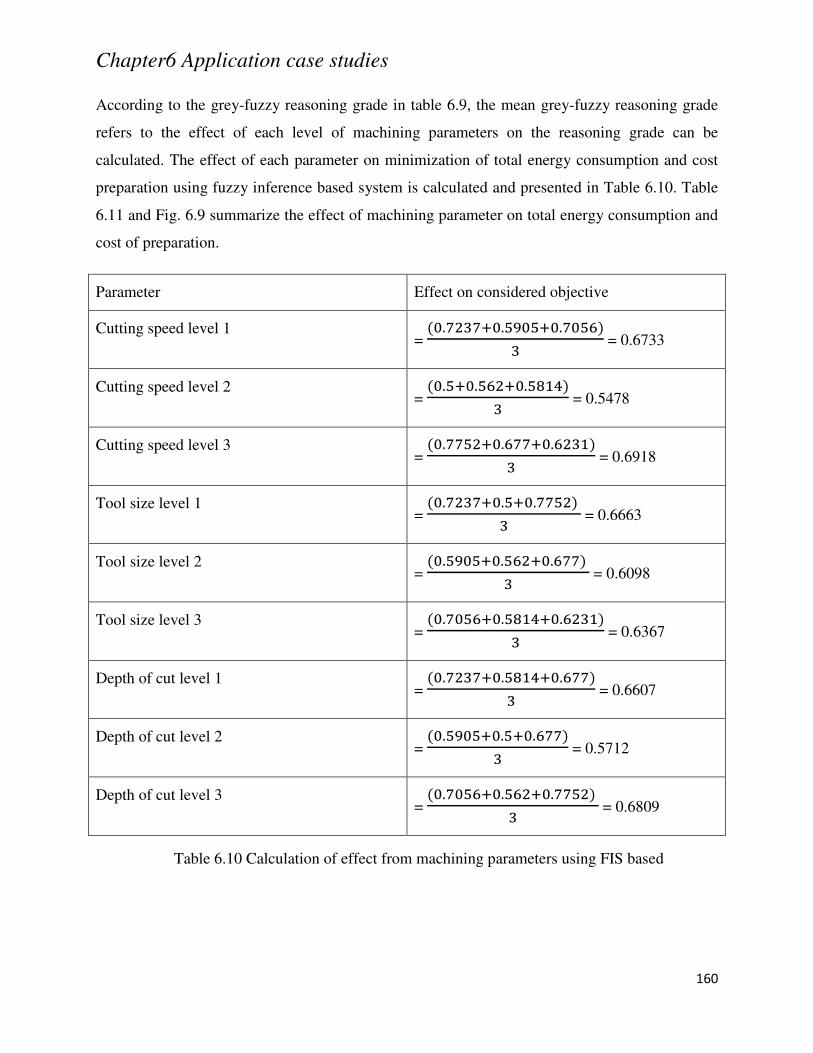
Chapter6 Application case studies
160
According to the grey-fuzzy reasoning grade in table 6.9, the mean grey-fuzzy reasoning grade
refers to the effect of each level of machining parameters on the reasoning grade can be
calculated. The effect of each parameter on minimization of total energy consumption and cost
preparation using fuzzy inference based system is calculated and presented in Table 6.10. Table
6.11 and Fig. 6.9 summarize the effect of machining parameter on total energy consumption and
cost of preparation.
Parameter Effect on considered objective
Cutting speed level 1 = Y.qY.XYXqY.YX = 0.6733
Cutting speed level 2 = Y.XqY.XqY.X = 0.5478
Cutting speed level 3 = Y.XqY.qY. = 0.6918
Tool size level 1 = Y.qY.XqY.X = 0.6663
Tool size level 2 = Y.XYXqY.XqY. = 0.6098
Tool size level 3 = Y.YXqY.XqY. = 0.6367
Depth of cut level 1 = Y.qY.XqY. = 0.6607
Depth of cut level 2 = Y.XYXqY.XqY. = 0.5712
Depth of cut level 3 = Y.YXqY.XqY.X = 0.6809
Table 6.10 Calculation of effect from machining parameters using FIS based
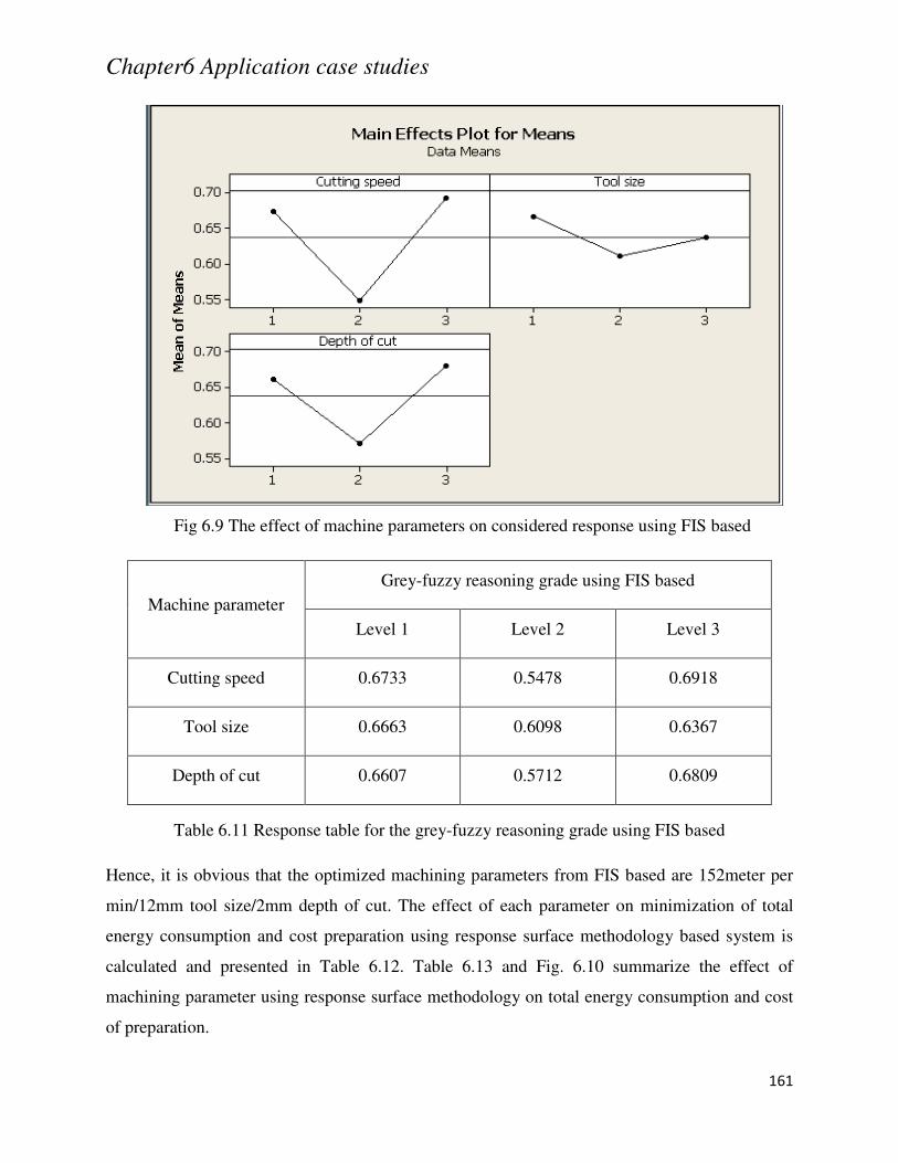
Chapter6 Application case studies
161
Fig 6.9 The effect of machine parameters on considered response using FIS based
Machine parameter
Grey-fuzzy reasoning grade using FIS based
Level 1 Level 2 Level 3
Cutting speed 0.6733 0.5478 0.6918
Tool size 0.6663 0.6098 0.6367
Depth of cut 0.6607 0.5712 0.6809
Table 6.11 Response table for the grey-fuzzy reasoning grade using FIS based
Hence, it is obvious that the optimized machining parameters from FIS based are 152meter per
min/12mm tool size/2mm depth of cut. The effect of each parameter on minimization of total
energy consumption and cost preparation using response surface methodology based system is
calculated and presented in Table 6.12. Table 6.13 and Fig. 6.10 summarize the effect of
machining parameter using response surface methodology on total energy consumption and cost
of preparation.
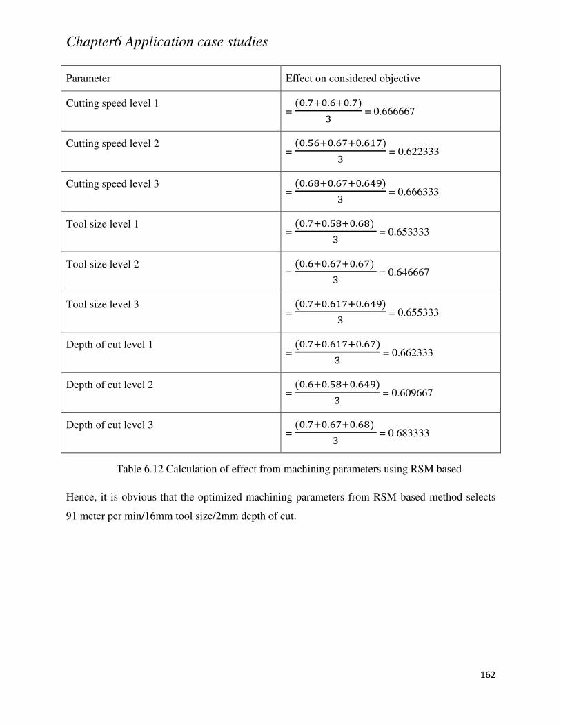
Chapter6 Application case studies
162
Parameter Effect on considered objective
Cutting speed level 1 = Y.qY.qY. = 0.666667
Cutting speed level 2 = Y.XqY.qY. = 0.622333
Cutting speed level 3 = Y.qY.qY. = 0.666333
Tool size level 1 = Y.qY.XqY. = 0.653333
Tool size level 2 = Y.qY.qY. = 0.646667
Tool size level 3 = Y.qY.qY. = 0.655333
Depth of cut level 1 = Y.qY.qY. = 0.662333
Depth of cut level 2 = Y.qY.XqY. = 0.609667
Depth of cut level 3 = Y.qY.qY. = 0.683333
Table 6.12 Calculation of effect from machining parameters using RSM based
Hence, it is obvious that the optimized machining parameters from RSM based method selects
91 meter per min/16mm tool size/2mm depth of cut.

Chapter6 Application case studies
163
Fig 6.10 The effect of machine parameters on considered response using RSM based
Machine parameter Grey-fuzzy reasoning grade using RSM based
Level 1 Level 2 Level 3
Cutting speed 0.666667 0.622333 0.666333
Tool size 0.653333 0.646667 0.655333
Depth of cut 0.662333 0.609667 0.683333
Table 6.13 Response table for the grey-fuzzy reasoning grade using RSM based
6.2.7 Analysis of energy efficiency and carbon footprint
To analyze the effect on energy efficiency and the carbon footprint from different two different
scenarios: 152 meter per min/12mm tool size/2mm depth of cut (scenario 1) and 91 meter per
min/16mm tool size/2mm depth of cut (scenario 2), the case of performing workpiece cutting for
one year is provided with experimental data (energy consumption). The results are illustrated in
Table 6.14 and the details of the cutting trial cases are:
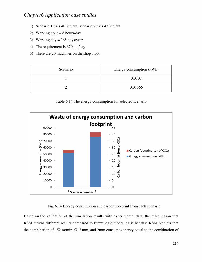
Chapter6 Application case studies
164
1) Scenario 1 uses 40 sec/cut, scenario 2 uses 43 sec/cut
2) Working hour = 8 hours/day
3) Working day = 365 days/year
4) The requirement is 670 cut/day
5) There are 20 machines on the shop-floor
Scenario Energy consumption (kWh)
1 0.0107
2 0.01566
Table 6.14 The energy consumption for selected scenario
Fig. 6.14 Energy consumption and carbon footprint from each scenario
Based on the validation of the simulation results with experimental data, the main reason that
RSM returns different results compared to fuzzy logic modelling is because RSM predicts that
the combination of 152 m/min, Ø12 mm, and 2mm consumes energy equal to the combination of
0
10000
20000
30000
40000
50000
60000
70000
80000
90000
1 2
0
5
10
15
20
25
30
35
40
45
En
erg
y c
on
smp
tio
n (
kW
h)
Scenario number
Ca
rbo
n f
oo
tpri
nt
(to
n o
f C
O2
)Waste of energy consumption and carbon
footprint
Carbon footprint (ton of CO2)
Energy consumption (kWh)
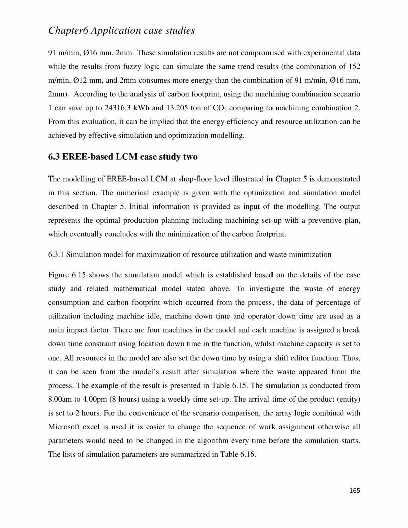
Chapter6 Application case studies
165
91 m/min, Ø16 mm, 2mm. These simulation results are not compromised with experimental data
while the results from fuzzy logic can simulate the same trend results (the combination of 152
m/min, Ø12 mm, and 2mm consumes more energy than the combination of 91 m/min, Ø16 mm,
2mm). According to the analysis of carbon footprint, using the machining combination scenario
1 can save up to 24316.3 kWh and 13.205 ton of CO2 comparing to machining combination 2.
From this evaluation, it can be implied that the energy efficiency and resource utilization can be
achieved by effective simulation and optimization modelling.
6.3 EREE-based LCM case study two
The modelling of EREE-based LCM at shop-floor level illustrated in Chapter 5 is demonstrated
in this section. The numerical example is given with the optimization and simulation model
described in Chapter 5. Initial information is provided as input of the modelling. The output
represents the optimal production planning including machining set-up with a preventive plan,
which eventually concludes with the minimization of the carbon footprint.
6.3.1 Simulation model for maximization of resource utilization and waste minimization
Figure 6.15 shows the simulation model which is established based on the details of the case
study and related mathematical model stated above. To investigate the waste of energy
consumption and carbon footprint which occurred from the process, the data of percentage of
utilization including machine idle, machine down time and operator down time are used as a
main impact factor. There are four machines in the model and each machine is assigned a break
down time constraint using location down time in the function, whilst machine capacity is set to
one. All resources in the model are also set the down time by using a shift editor function. Thus,
it can be seen from the model’s result after simulation where the waste appeared from the
process. The example of the result is presented in Table 6.15. The simulation is conducted from
8.00am to 4.00pm (8 hours) using a weekly time set-up. The arrival time of the product (entity)
is set to 2 hours. For the convenience of the scenario comparison, the array logic combined with
Microsoft excel is used it is easier to change the sequence of work assignment otherwise all
parameters would need to be changed in the algorithm every time before the simulation starts.
The lists of simulation parameters are summarized in Table 6.16.
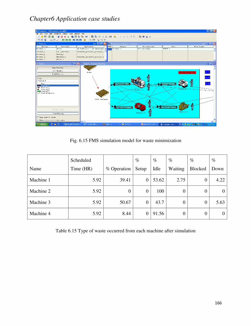
Chapter6 Application case studies
166
Fig. 6.15 FMS simulation model for waste minimization
Name
Scheduled
Time (HR) % Operation
%
Setup
%
Idle
%
Waiting
%
Blocked
%
Down
Machine 1 5.92 39.41 0 53.62 2.75 0 4.22
Machine 2 5.92 0 0 100 0 0 0
Machine 3 5.92 50.67 0 43.7 0 0 5.63
Machine 4 5.92 8.44 0 91.56 0 0 0
Table 6.15 Type of waste occurred from each machine after simulation
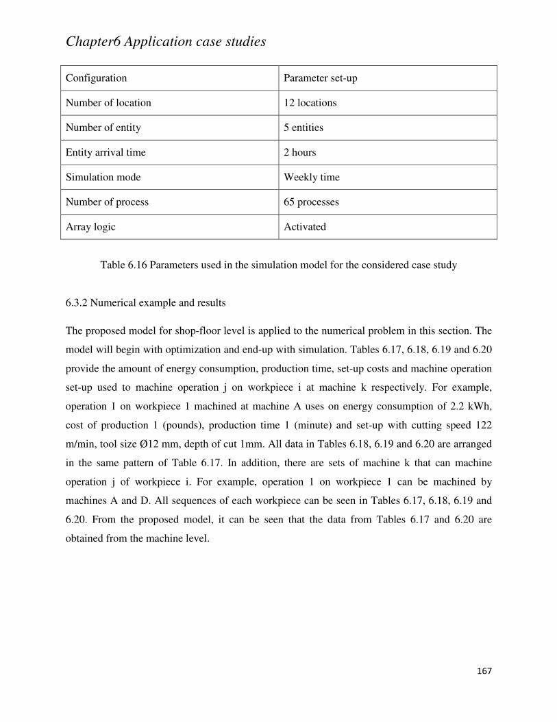
Chapter6 Application case studies
167
Configuration Parameter set-up
Number of location 12 locations
Number of entity 5 entities
Entity arrival time 2 hours
Simulation mode Weekly time
Number of process 65 processes
Array logic Activated
Table 6.16 Parameters used in the simulation model for the considered case study
6.3.2 Numerical example and results
The proposed model for shop-floor level is applied to the numerical problem in this section. The
model will begin with optimization and end-up with simulation. Tables 6.17, 6.18, 6.19 and 6.20
provide the amount of energy consumption, production time, set-up costs and machine operation
set-up used to machine operation j on workpiece i at machine k respectively. For example,
operation 1 on workpiece 1 machined at machine A uses on energy consumption of 2.2 kWh,
cost of production 1 (pounds), production time 1 (minute) and set-up with cutting speed 122
m/min, tool size Ø12 mm, depth of cut 1mm. All data in Tables 6.18, 6.19 and 6.20 are arranged
in the same pattern of Table 6.17. In addition, there are sets of machine k that can machine
operation j of workpiece i. For example, operation 1 on workpiece 1 can be machined by
machines A and D. All sequences of each workpiece can be seen in Tables 6.17, 6.18, 6.19 and
6.20. From the proposed model, it can be seen that the data from Tables 6.17 and 6.20 are
obtained from the machine level.
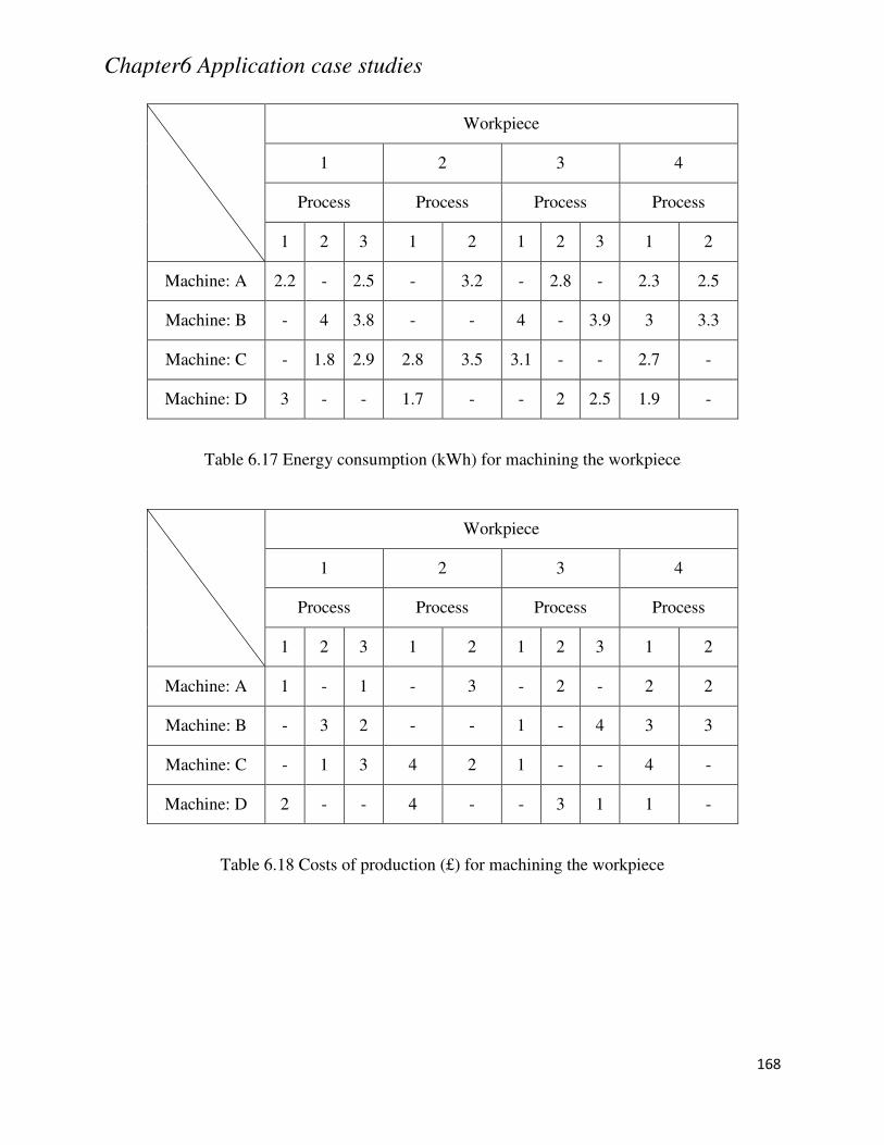
Chapter6 Application case studies
168
Workpiece
1 2 3 4
Process Process Process Process
1 2 3 1 2 1 2 3 1 2
Machine: A 2.2 - 2.5 - 3.2 - 2.8 - 2.3 2.5
Machine: B - 4 3.8 - - 4 - 3.9 3 3.3
Machine: C - 1.8 2.9 2.8 3.5 3.1 - - 2.7 -
Machine: D 3 - - 1.7 - - 2 2.5 1.9 -
Table 6.17 Energy consumption (kWh) for machining the workpiece
Workpiece
1 2 3 4
Process Process Process Process
1 2 3 1 2 1 2 3 1 2
Machine: A 1 - 1 - 3 - 2 - 2 2
Machine: B - 3 2 - - 1 - 4 3 3
Machine: C - 1 3 4 2 1 - - 4 -
Machine: D 2 - - 4 - - 3 1 1 -
Table 6.18 Costs of production (£) for machining the workpiece
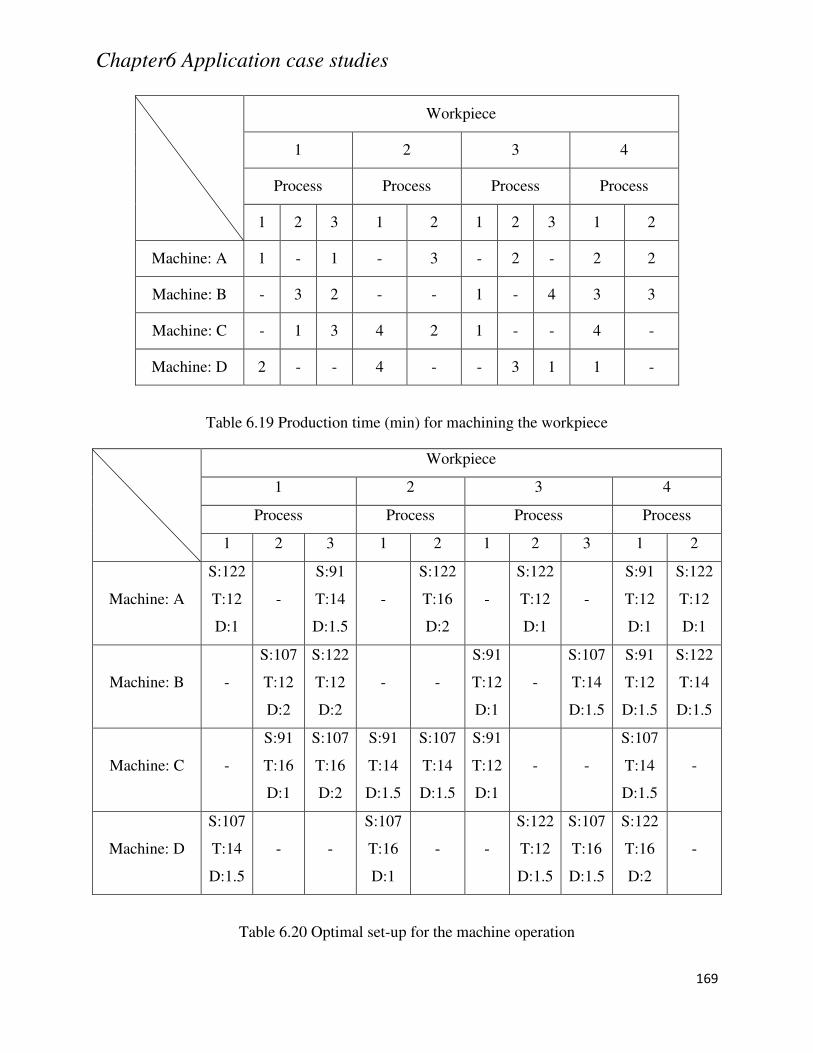
Chapter6 Application case studies
169
Workpiece
1 2 3 4
Process Process Process Process
1 2 3 1 2 1 2 3 1 2
Machine: A 1 - 1 - 3 - 2 - 2 2
Machine: B - 3 2 - - 1 - 4 3 3
Machine: C - 1 3 4 2 1 - - 4 -
Machine: D 2 - - 4 - - 3 1 1 -
Table 6.19 Production time (min) for machining the workpiece
Workpiece
1 2 3 4
Process Process Process Process
1 2 3 1 2 1 2 3 1 2
Machine: A
S:122
T:12
D:1
-
S:91
T:14
D:1.5
-
S:122
T:16
D:2
-
S:122
T:12
D:1
-
S:91
T:12
D:1
S:122
T:12
D:1
Machine: B -
S:107
T:12
D:2
S:122
T:12
D:2
- -
S:91
T:12
D:1
-
S:107
T:14
D:1.5
S:91
T:12
D:1.5
S:122
T:14
D:1.5
Machine: C -
S:91
T:16
D:1
S:107
T:16
D:2
S:91
T:14
D:1.5
S:107
T:14
D:1.5
S:91
T:12
D:1
- -
S:107
T:14
D:1.5
-
Machine: D
S:107
T:14
D:1.5
- -
S:107
T:16
D:1
- -
S:122
T:12
D:1.5
S:107
T:16
D:1.5
S:122
T:16
D:2
-
Table 6.20 Optimal set-up for the machine operation
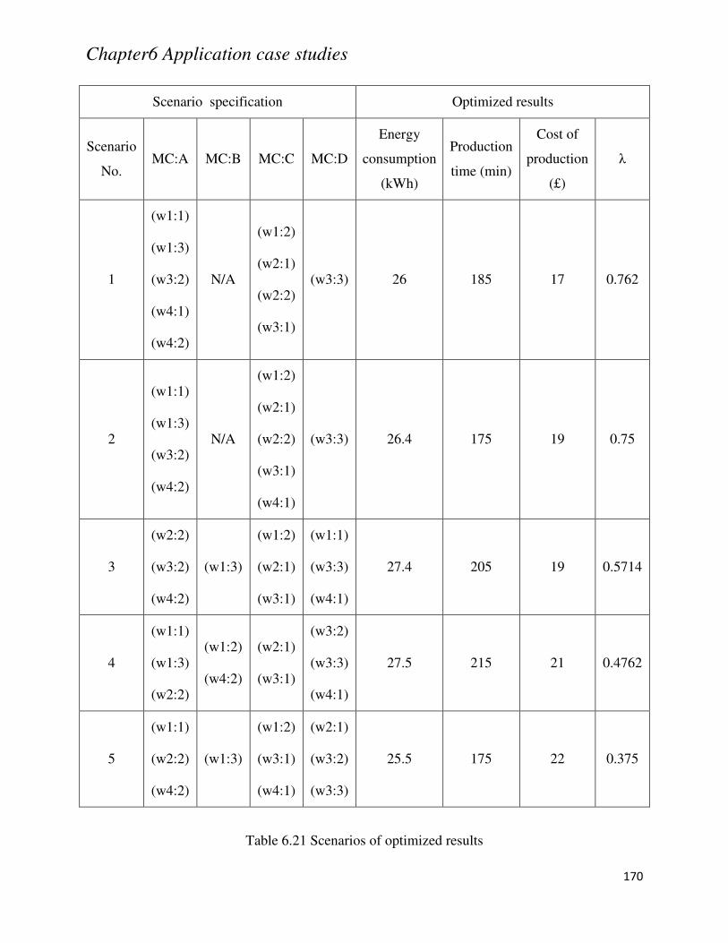
Chapter6 Application case studies
170
Scenario specification Optimized results
Scenario
No. MC:A MC:B MC:C MC:D
Energy
consumption
(kWh)
Production
time (min)
Cost of
production
(£)
λ
1
(w1:1)
(w1:3)
(w3:2)
(w4:1)
(w4:2)
N/A
(w1:2)
(w2:1)
(w2:2)
(w3:1)
(w3:3) 26 185 17 0.762
2
(w1:1)
(w1:3)
(w3:2)
(w4:2)
N/A
(w1:2)
(w2:1)
(w2:2)
(w3:1)
(w4:1)
(w3:3) 26.4 175 19 0.75
3
(w2:2)
(w3:2)
(w4:2)
(w1:3)
(w1:2)
(w2:1)
(w3:1)
(w1:1)
(w3:3)
(w4:1)
27.4 205 19 0.5714
4
(w1:1)
(w1:3)
(w2:2)
(w1:2)
(w4:2)
(w2:1)
(w3:1)
(w3:2)
(w3:3)
(w4:1)
27.5 215 21 0.4762
5
(w1:1)
(w2:2)
(w4:2)
(w1:3)
(w1:2)
(w3:1)
(w4:1)
(w2:1)
(w3:2)
(w3:3)
25.5 175 22 0.375
Table 6.21 Scenarios of optimized results
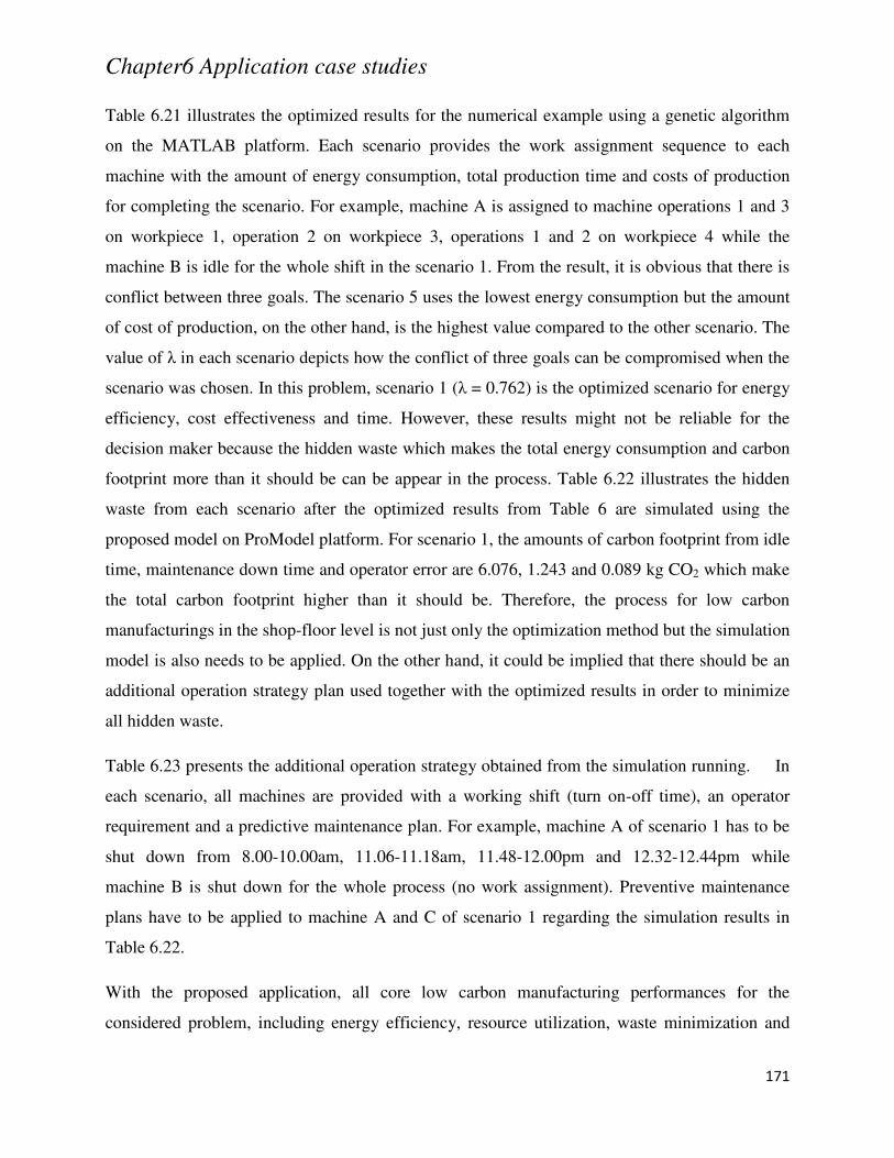
Chapter6 Application case studies
171
Table 6.21 illustrates the optimized results for the numerical example using a genetic algorithm
on the MATLAB platform. Each scenario provides the work assignment sequence to each
machine with the amount of energy consumption, total production time and costs of production
for completing the scenario. For example, machine A is assigned to machine operations 1 and 3
on workpiece 1, operation 2 on workpiece 3, operations 1 and 2 on workpiece 4 while the
machine B is idle for the whole shift in the scenario 1. From the result, it is obvious that there is
conflict between three goals. The scenario 5 uses the lowest energy consumption but the amount
of cost of production, on the other hand, is the highest value compared to the other scenario. The
value of λ in each scenario depicts how the conflict of three goals can be compromised when the
scenario was chosen. In this problem, scenario 1 (λ = 0.762) is the optimized scenario for energy
efficiency, cost effectiveness and time. However, these results might not be reliable for the
decision maker because the hidden waste which makes the total energy consumption and carbon
footprint more than it should be can be appear in the process. Table 6.22 illustrates the hidden
waste from each scenario after the optimized results from Table 6 are simulated using the
proposed model on ProModel platform. For scenario 1, the amounts of carbon footprint from idle
time, maintenance down time and operator error are 6.076, 1.243 and 0.089 kg CO2 which make
the total carbon footprint higher than it should be. Therefore, the process for low carbon
manufacturings in the shop-floor level is not just only the optimization method but the simulation
model is also needs to be applied. On the other hand, it could be implied that there should be an
additional operation strategy plan used together with the optimized results in order to minimize
all hidden waste.
Table 6.23 presents the additional operation strategy obtained from the simulation running. In
each scenario, all machines are provided with a working shift (turn on-off time), an operator
requirement and a predictive maintenance plan. For example, machine A of scenario 1 has to be
shut down from 8.00-10.00am, 11.06-11.18am, 11.48-12.00pm and 12.32-12.44pm while
machine B is shut down for the whole process (no work assignment). Preventive maintenance
plans have to be applied to machine A and C of scenario 1 regarding the simulation results in
Table 6.22.
With the proposed application, all core low carbon manufacturing performances for the
considered problem, including energy efficiency, resource utilization, waste minimization and
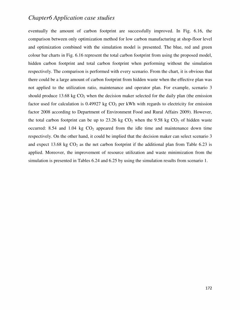
Chapter6 Application case studies
172
eventually the amount of carbon footprint are successfully improved. In Fig. 6.16, the
comparison between only optimization method for low carbon manufacturing at shop-floor level
and optimization combined with the simulation model is presented. The blue, red and green
colour bar charts in Fig. 6.16 represent the total carbon footprint from using the proposed model,
hidden carbon footprint and total carbon footprint when performing without the simulation
respectively. The comparison is performed with every scenario. From the chart, it is obvious that
there could be a large amount of carbon footprint from hidden waste when the effective plan was
not applied to the utilization ratio, maintenance and operator plan. For example, scenario 3
should produce 13.68 kg CO2 when the decision maker selected for the daily plan (the emission
factor used for calculation is 0.49927 kg CO2 per kWh with regards to electricity for emission
factor 2008 according to Department of Environment Food and Rural Affairs 2009). However,
the total carbon footprint can be up to 23.26 kg CO2 when the 9.58 kg CO2 of hidden waste
occurred: 8.54 and 1.04 kg CO2 appeared from the idle time and maintenance down time
respectively. On the other hand, it could be implied that the decision maker can select scenario 3
and expect 13.68 kg CO2 as the net carbon footprint if the additional plan from Table 6.23 is
applied. Moreover, the improvement of resource utilization and waste minimization from the
simulation is presented in Tables 6.24 and 6.25 by using the simulation results from scenario 1.
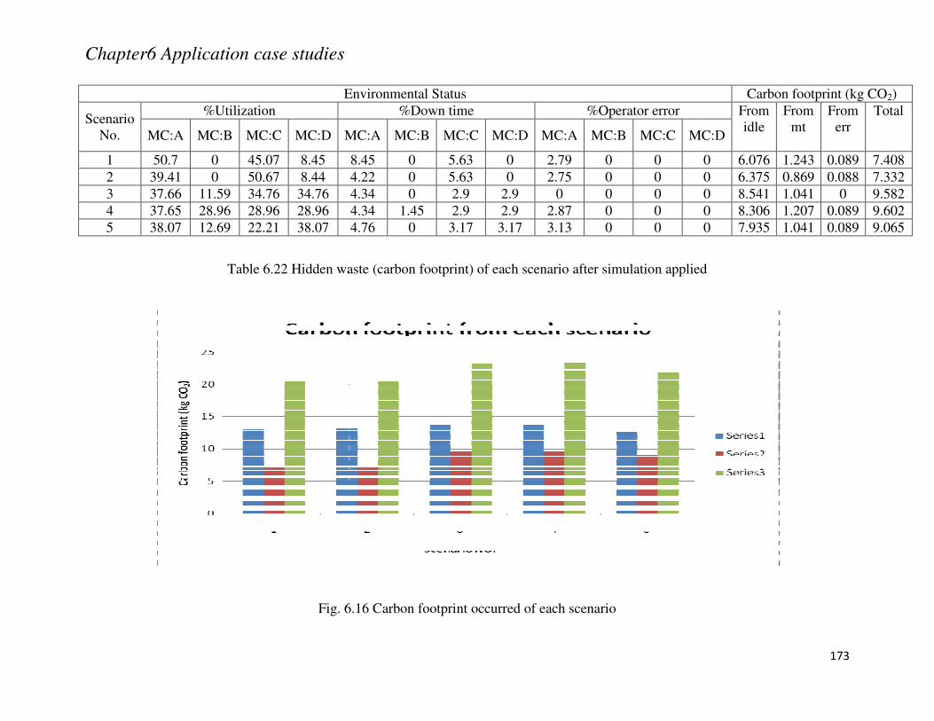
Chapter6 Application case studies
Environmental Status
Scenario No.
%Utilization
MC:A MC:B MC:C MC:D MC:A
1 50.7 0 45.07 8.45
2 39.41 0 50.67 8.44 3 37.66 11.59 34.76 34.76 4 37.65 28.96 28.96 28.96
5 38.07 12.69 22.21 38.07
Table 6.22 Hidden waste (carbon footprint)
Fig. 6.16
Environmental Status %Down time %Operator error
MC:A MC:B MC:C MC:D MC:A MC:B MC:C MC:D
8.45 0 5.63 0 2.79 0 0
4.22 0 5.63 0 2.75 0 0 4.34 0 2.9 2.9 0 0 0 4.34 1.45 2.9 2.9 2.87 0 0
4.76 0 3.17 3.17 3.13 0 0
Hidden waste (carbon footprint) of each scenario after simulation applied
Fig. 6.16 Carbon footprint occurred of each scenario
173
Carbon footprint (kg CO2) From idle
From mt
From err
Total
MC:D
0 6.076 1.243 0.089 7.408
0 6.375 0.869 0.088 7.332 0 8.541 1.041 0 9.582 0 8.306 1.207 0.089 9.602
0 7.935 1.041 0.089 9.065
each scenario after simulation applied

Chapter6 Application case studies
174
Scenario NO. Scheduling time (turn off) Operator
requirement Maintenance
MC:A MC:B MC:C MC:D
1
8.00 – 10.00 am
11.06 – 11.18 am
11.48 – 12.00 am
12.32 – 12.44 pm
N/Aa
8.00 – 10.00 am
11.24 – 12.00 am
13.24 – 14.00 pm
8.00 – 10.44 am
11.02 – 13.00 pm
13.16 – 14.00 pm
2 for MC:Ab
1 for MC:B
1 for MC:C
1 for MC:D
Preventive
maintenance for
MC:A and C
2
8.00 – 10.00 am
10.11 – 10.14 am
10.32 – 11.00 am
11.46 – 12.00 am
12.11 – 12.14 pm
12.32 – 13.06 pm
N/A
8.00 – 10.00 am
11.11 – 11.19 am
11.41 – 12.00 am
12.51 – 13.00 pm
13.41 – 14.00 pm
8.00 – 10.30 am
10.47 – 12.30 pm
12.47 – 14.00 pm
2 for MC:A
1 for MC:B
1 for MC:C
1 for MC:D
Preventive
maintenance for
MC:A and C
3
8.00 – 10.14 am
10.32 – 10.44 am
11.36 – 12.12 pm
12.32 – 12.54 pm
8.00 – 11.00 am
11.22 – 13.09 pm
13.31 – 14.00 pm
8.00 – 10.00 am
11.01 – 12.00 am
12.16 – 12.24 pm
13.12 – 14.00 pm
8.00 – 10.00 am
11.01 – 12.00 am
12.31 – 12.39 pm
13.11 – 14.00 pm
1 for MC:A
1 for MC:B
1 for MC:C
1 for MC:D
Preventive
maintenance for
MC:A, C and D
4
8.00 – 10.00 am
10.11 – 10.30 am
11.27 – 12.00 am
12.11 – 12.30 pm
8.00 – 10.09 am
11.01 – 12.09 pm
13.01 – 14.00 pm
8.00 – 10.00 am
10.51 – 12.00 am
12.51 – 14.00 pm
8.00 – 10.00 am
10.52 – 12.00 am
12.36 – 12.44 pm
13.01 – 14.00 pm
2 for MC:A
1 for MC:B
1 for MC:C
1 for MC:D
Preventive
maintenance for
MC:A, B, C and D
5
8.00 – 10.00 am
10.11 – 10.24 am
11.16 – 12.00 am
12.11 – 12.24 pm
8.00 – 10.34 am
10.57 – 12.34 pm
12.57 – 14.00 pm
8.00 – 10.00 am
10.36 – 12.00 am
12.36 – 14.00 pm
8.00 – 10.00 am
11.01 – 12.00 am
12.27 – 12.34 pm
13.11 – 14.00 pm
2 for MC:A
1 for MC:B
1 for MC:C
1 for MC:D
Preventive
maintenance for
MC:A, C and D
Table 6.23 The operational strategy applied to each scenario to reduce waste at shop-floor level
aMachine B must be turn off for the whole working period
bMachine A requires 2 operators for the whole working period
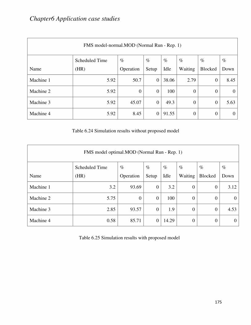
Chapter6 Application case studies
175
FMS model-normal.MOD (Normal Run - Rep. 1)
Name
Scheduled Time
(HR)
%
Operation
%
Setup
%
Idle
%
Waiting
%
Blocked
%
Down
Machine 1 5.92 50.7 0 38.06 2.79 0 8.45
Machine 2 5.92 0 0 100 0 0 0
Machine 3 5.92 45.07 0 49.3 0 0 5.63
Machine 4 5.92 8.45 0 91.55 0 0 0
Table 6.24 Simulation results without proposed model
FMS model optimal.MOD (Normal Run - Rep. 1)
Name
Scheduled Time
(HR)
%
Operation
%
Setup
%
Idle
%
Waiting
%
Blocked
%
Down
Machine 1 3.2 93.69 0 3.2 0 0 3.12
Machine 2 5.75 0 0 100 0 0 0
Machine 3 2.85 93.57 0 1.9 0 0 4.53
Machine 4 0.58 85.71 0 14.29 0 0 0
Table 6.25 Simulation results with proposed model

Chapter6 Application case studies
176
6.4 Summary
The feasibility of EREE-based LCM models has been demonstrated with two case studies,
although there is still a long way to go to develop the comprehensive EREE-based LCM because
there are enterprise and supply levels that are also required to develop the feasible modelling.
The case studies have only validated the modelling for both the machine and shop-floor levels.
The case study one is validated using experimental results while the case study two is validated
by using simulation results.
Chapter7 Conclusions and recommendations for future work
177
Chapter 7 Conclusions and recommendations for future work
This chapter draws important conclusions of the investigations, highlights the contributions to
knowledge, and recommends the work for future studies.
7.1 Conclusions
Based upon the discussion in the previous chapters and results from the investigations,
the following conclusions can be drawn:
1) Under the great impact of the new manufacturing platform which includes sustainable
development as a manufacturing performance, the continuing development of systematic
approaches for integrating carbon footprint reduction aspect with typical manufacturing
performances has made it necessary and possible to develop “Energy Resource
Efficiency and Effectiveness based Low Carbon Manufacturing (EREE-based LCM)”.
The development of EREE-based LCM demonstrates the potential to offer energy
efficiency, resource utilization, waste minimization and even reduction of the carbon
footprint for the different manufacturing levels such as machine and shop-floor level.
2) In order to scientifically organize and manage the complexities involved in EREE-based
LCM, an integrated framework, theoretical model and characterizations have been
proposed to support LCM development. In the proposed framework, the
recommendations to achieve EREE-based LCM for each manufacturing level have been
demonstrated.
3) To design a systematical approach, the axiomatic design is used to integrate
characterizations of EREE-based LCM including energy efficiency, resource utilization
and waste minimization to satisfy the main functional requirement (reduction of carbon
footprint). It can be concluded that as conceptual design of the systematical approach can
be applied to different manufacturing levels.
4) At machine level, the proposed modelling demonstrated its ability to provide a machining
set-up that includes energy efficiency and resource utilization. The simulation of energy
consumption affected by cutting parameters and selected resources has been implemented
using sugeno-type fuzzy logic while the optimization of the machining set-up is
implemented using a grey relational based fuzzy logic model (mamdani type fuzzy logic).
Chapter7 Conclusions and recommendations for future work
178
The user interface using MATLAB GUI is developed to control the two different types of
fuzzy inference engine.
5) At the shop-floor level, the process of combining the mathematical optimization model
with the results from the machine level has been introduced in the form of a profile
matrix. Fuzzy integer linear programming with several objectives is used to formulate
mathematical model for providing the optimal results of energy efficiency and resource
utilization. To solve the problem, the genetic algorithm toolbox in MATLAB is used.
6) The waste elimination model used to reduce wastes that affect the amount of carbon
footprint has been developed on the ProModel platform. Discrete event simulation theory
is used to simulate wastes from machine idle time, human error and maintenance down
time. The input of this model is the optimal results from the optimization model while the
output is a preventive plan used together with the optimal results in order to eliminate an
unnecessary carbon footprint and increase the reliability of the optimal result.
7.2 Contributions to knowledge
1) A novel energy resource efficiency and effectiveness based low carbon manufacturing
(EREE-based LCM) has been proposed, and a framework and methodologies have been
established, designed and demonstrated.
2) For the first time, the axiomatic design theory is applied to design a systematical
approach for achieving low carbon emissions by integrating energy efficiency, resource
utilization and waste minimization together.
3) An integrated tool box for the simulation of the energy consumption of a machining
cutting process is developed using a sugeno-type fuzzy inference engine while the
optimization process is conducted using a mamdani-type fuzzy inference engine. This
support system includes user-friendly interface (MATLAB GUI), learning/rule base
simulation and optimization with interpretation of results
4) The profile matrix is developed to synchronize results from the machine level with the
optimization model of the shop-floor level. Thus, optimal results at shopfloor level can
provide production plan with energy efficiency and optimized resource planning.
5) The waste elimination model is proposed using a time based simulation method via
ProModel discrete event system simulation platform. The model can evaluate results
Chapter7 Conclusions and recommendations for future work
179
from the optimization model and eliminate the waste/unnecessary of energy consumption
and the carbon footprint from manufacturing process.
7.3 Recommendations for future work
Since the research covers the range of aspects related to the development of EREE-based low
carbon manufacturing, there are relevant contexts in the proposed concept which are
incompletely investigated due to the limit of time and available facilities. The following areas are
thus recommended for future investigations:
1) For the implementation of EREE-based LCM at shop-floor level, it is possible to develop
the user interface such as Visulabasic based to control the optimization in MATLAB and
the simulation model in ProModel together.
2) The mathematical model used for optimizing the resources and energy profile can be
developed in terms of both mathematical function and seeking procedure. These additions
can return the compatibility of complex system and the high potential of finding a global
solution.
3) To improve the accuracy of the simulation model at shop-floor level, the validation of
data distributions used in the model must be taken based on the comparison of simulation
results and experimental data. The effectiveness of waste elimination can be, thus,
improved.
4) More mathematical functions can be added into the learning process of Sugeno type
fuzzy logic to provide more alternatives of membership function selection. The
simulation results of energy consumption can be, thus, improved.
5) According to the model at machine level, the data from the commercial sector such as the
machine provider can be added to the model as a reference base to compare with the
formulated function created by fuzzy logic.
References
180
References
Ahilan, C., Kumana, S., and Sivakumaran, N. (2009). "Multi-objective optimization of CNC
turning process using grey based fuzzy logic." International Journal of Machining and
Machinability of Materials 5(4): 434-451.
Allen, J., Browne, M., Hunter, A., Boyd, J., and Palmer, H. (1998). "Logistics management and
costs of biomass fuel supply." International Journal of Physical Distribution and Logistics
Management 28(6): 463-477.
Antony, J. (2001). "Simultaneous optimisation of multiple quality characteristics in
manufacturing processes using Taguchi's quality loss function." International Journal of
Advanced Manufacturing Technology 17: 134-138.
Askin, R. G., and Standridge, C.R. (1993). Modeling and Analysis of Manufacturing Systems,
John Wiley & Sons, Inc.
Azapagic, A., and Perdan, S. (2010). Sustainable Development in Practice: Case Studies for
Engineers and Scientists, Wiley.
Ball, P. D., Evans, S., Lever, A., and Ellison, D. (2009). "Zero carbon manufacturing facility-
towards integrating material, energy and waste process flows." Proceedings of the Institution of
Mechanical Engineers, Part B: Journal of Engineering Manufacture 223: 1085-1096.
Bateman, J. R., and Cheng, K. (2002). "Devolved Manufacturing: theoretical perspectives."
Concurrent Engineering: Research and Applications 10(4): 291-297.
References
181
Bateman, J. R., and Cheng, K. (2006). "Extending the product portfolio with devolved
manufacturing: methodology and case studies." International Journal of Production Research
44(16): 3325-3343.
Beek, P., Fortuin, L., and Wassenhove, L. (1992). "Operation research and the environment."
Environmental and Resource Economics 2(6): 635-639.
Bhamra, T. (2007). Design for sustainability: a practical approach, Gower.
Bloemhof-Ruwaard, J. M., Beek, P.V., Hordijk, L., and Wassenhove, L.N.V. (1995).
"Interactions between operational research and environmental management." European Journal
of Operational Research 85: 229-243.
Bloemhof-Ruwaard, J. M., Koudijs, H.G., and Vis, J.C. (1995). "Environmental Impacts of Fat
Blends: A Methodological Study Combining Life Cycle Analysis, Multiple Criteria Decision
Making and Linear Programming." Environmental and Resource Economics 6: 371-387.
British Standards Institute (2004). Environmental management systems-Requirements with
guidance for use (ISO 14001:2004).
British Standards Institute (2008). PAS 2050-Specification for the assessment of the life cycle
green house gas emissions of goods and services.
References
182
Byrne, G., and Scholta, E. (1993). "Environmentally clean machining process-a strategic
approach." Annals of the CIRP 42(1): 471-474.
Chai, Q., and Zhang, X. (2010). "Technologies and policies for the transition to a sustainable
energy system in china." Energy 35: 3995-4002.
Chang Ching-Kao, H. S. L. (2007). "The optimal cutting-parameter selection of heavy cutting
process in side milling for SUS304 stainless steel." The International Journal of Advanced
Manufacturing Technology 34: 440-447.
Cheng, K., and Bateman, J. (2008). "e-Manufacturing: characteristics, applications and
potentials." Progress in Natural Science 18: 1323-1328.
Chin-Tsai L., C.-B., C., and Ying-Chan, T. (2011). "An ERP model for supplier selection in
electronics industry." Expert Systems with Applications 38: 1760-1765.
Cristobal, J. R. (2011). "Multi-criteria decision-making in the selection of renewable energy
project in Spain: the vikor method." Renewable Energy 36: 498-502.
Dahmus, B. J., and Gutowski, T.G. (2004). "An environmental analysis of machining."
Proceedings of IMECE2004: 1-10.
Davis, J. W. (1999). Fast Track to Waste-Free manufacturing: Straight Talk from a Plant
Manager, Portland, Productivity Press.
References
183
Deng, J. (1989). "Introduction to grey system." The Journal of Grey System 1: 1–24.
Department for Business Enterprise and Regulatory Reform and Department of Energy and
Climate Change (2009). Low Carbon Industrial Strategy: A vision.
Department for Environment Food and Rural Affair (DEFRA) (2009). Guidelines to DEFRA/
DECC’s GHG Converion Factors for Company Reporting.
Department of Energy and Climate Change (DECC) (2008). Local and Regional CO2 Emissions
Estimates for 2005 - 2008 for the UK, Department of Energy and Climate Change.
Department of Energy and Climate Change (DECC) (2009). Digest of United Kingdom Energy
Statistics 2009.
Department of Energy and Climate Change (DECC) (2009). Summary of responses to the
consultation on carbon units, the net UK carbon account and carbon accounting held between 28
October 2008 and 19 January 2009.
Diesendorf, M. (2007). Greenhouse Solutions with Sustainable Energy. Sydney, UNSW Press.
Dweiri, F., Al-Jarrah, M., and Al-Wedyan H. (2003). "Fuzzy surface roughness modeling of
CNC down milling of Alumic-79." Journal of Machining Processing Technology 33: 266-275.
Eastop, T. D., and Croft, D.R. (1990). Energy efficiency for engineers and technologists. UK,
Longman Group UK Ltd.
References
184
Edwards, E. E., Iyare, O.S., and Moseley, L.L. (2012). "Energy consumption in typical
Caribbean office buildings: A potential short term solution to energy concerns." Renewable
Energy 39: 154-161.
Elkington, J. (1997). Cannibals with forks: The triple bottom line of 21stcentury business.
Oxford, Capstone Publishing Ltd.
Erdogdu, E. (2010). "Turkish support to Kyoto Protocol: a reality or just an illusion." Renewable
and Sustainable Energy Reviews 14: 1111-1117.
Fan, Y., Liang, Q., We,i Y.. and Okada, N. (2007). "A model for China’s energy requirements
and CO2 emissions analysis." Environmental Modelling & Software 22: 378-393.
Faucheux, S., and Nicolai, I. (1998). "Environmental technological change and governance in
sustainable development policy." Ecological Economics 27: 243-256.
Flower, D. J. M., and Sanjayan, J. G. (2007). "Green house gas emissions due to concrete
manufacture." The International Journal of Life Cycle Assessment 12(5): 282-288.
Freris, L., and Infield, D. (2008). Renewable Energy in Power Systems, Wiley.
Gaitonde, V. N., Karmik, S.R., and Davim, J.P. (2008). "Taguchi multiple-performance
characteristics optimization in drilling of medium density fibreboard (MDF) to minimize
delamination using utility concept." Journal of Materials Processing Technology 196: 73-78.
References
185
Gold, S., and Seuring, S. (2011). "Supply chain and logistics issue of bio-energy production."
Journal of Cleaner Production 19: 32-42.
Golove, W. H., and Schipper, L. J. (1996). "Long-Term Trends in U.S. Manufacturing Energy
Consumption and Carbon Dioxide Emissions." Energy 21: 683-692.
Gungor, A., and Gupta, S.M. (1999). "Issues in environmentally conscious manufacturing and
product recover: a survey." Computers & Industrial Engineering 36: 811-853.
Gutowski, T., Dahmus, J., and Thiriez, A. (2006). Electrical energy requirements for
manufacturing processes. 13th CIRP International Conference on Life Cycle Engineering,
Leuven.
Haq, A. N., Marimuthu, P., and Jeyapaul, R. (2008). "Multi reponse optimization of machining
parameters of drilling Al/SiC metal matrix composite using grey relational analysis in the
Taguchi method." International Journal of Advanced Manufacturing Technology 37: 250-255.
Harrell, C., Ghosh, B. K., and Bowden, R. O. (2003). Simulation using ProMode. New York,
McGraw-Hill Inc.
Harvey-Tool (2011). "General Machining Guidelines." 2011, from
http://www.harveytool.com/cms/GeneralMachiningGuidelines_17.aspx.
References
186
Heilala, J., Vatanen, S., and Tonteri, H. et al (2008). "Simulation-based sustainable
manufacturing design." Proceedings of the 2008 Winter Simulation Conference: 1922-1930.
Herrmann, C., and Thiede, S. (2009). "Process chain simulation to foster energy efficiency in
manufacturing." CIRP Journal of Manufacturing Science and Technology 1: 221-229.
Hoicka, C. E., and Rowlands, I.H. (2011). "Solar and wind resource complementarity: advancing
options for renewable electricity integration in Ontario, Canada." Renewable Energy 36: 97-107.
Hughes, E. (2009). Electrical and electronic technology. United Kingdom, Pearson Education
UK.
Humphreys, P. K., Wong, Y.K., and Chan, F.T.S. (2003). "Integrating environmental criteria and
validation." Journal of Materials Processing Technology 138(1-3): 249-256.
Intergovermental Panel on Climate Change (IPCC) (1997). Implications of Proposed CO2
Emissions Limitations.
Intergovernmental Panel on Climate Change (IPCC) (2006). Revised 1996 IPCC Guidelines for
National Greenhouse Gas Inventories: Workbook.
Jabbour, A. B. L. S., and Jabbour, C.J.C. (2009). "Are supplier selection going green? case
studies of companies in Brazil." Industrial Management & Data Systems 100(4): 477-495.
References
187
Jeyapaul, R., Shahabudeen, P, and Krishnaiah, K. (2005). "Quality management research by
considering multi-response problems in the Taguchi methods-a review." International Journal of
Advanced Manufacturing Technology 26: 1331-1337.
Jovane, F., Yoshikawa, H., and Alting, L. et al (2008). "The incoming global technological and
industrial revolution towards competitive sustainable manufacturing." CIRP Annals-
Manufacturing Technology 57: 641-659.
Kline, W. A., and Devor, R.E. (1983). "The effect of runout on cutting geometry and forces in
end milling." International Journal of Machine Tool Design and Researh 23(2-3): 123-140.
Kline, W. A., Devor, R.E., and Linberg, J.R. (1982). "The prediction of cutting forces in end
milling with application to concerning cuts." International Journal of Machine Tool Design and
Research 22(1): 7-22.
Kone, A. C., and Buke, T. (2010). "Forecasting of CO2 emissions from fuel combustion using
trend analysis." Renewable and Sustainable Energy Reviews 14: 2906-2915.
Kosa, P., Kulworawanichpong, T., and Srivoramas, R. et al (2011). "The potential hydro micro-
power projects in Nakhon Ratchasima province, Thailand." Renewable Energy 36: 1133-1137.
Kuhtz, S., Zhou, C., and Albino, V. et al (2010). "Energy use in two Italian and Chinese tile
manufacturers: a comparison using an enterprise input-output model." Energy 35: 364-374.
Lai, W. (2000). "Modeling of Cutting Forces in End Milling Operations." Tamkang Journal of
Science and Engineering 3(1): 15-22.
References
188
Lau, H. C. W., Cheng, E.N.M., Lee, C.K.M., and Ho, G.T.S. (2008). "A fuzzy logic approach to
forecast energy consumption change in manufacturing system." Expert Systems with
Applications 34: 1813-1824.
Lin, J. L., and Lin, C.L. (2005). "The use of grey-fuzzy logic for the optimization of the
manufacturing process." Journal of Machining Processing Technology 160: 9-14.
Lin, J. L., Wang, K. S., Yan, B. H., and Tarng, Y. S. (2000). "Optimization of the electrical
discharge machining process based on the Taguchi method with fuzzy logics." Journal of
Materials Processing Technology 102: 48-55.
Lin, J. L., and Lin, C.L. (2005). "The use of grey-fuzzy logic for the optimization of the
manufacturing process." Journal of Machining Processing Technology 160: 9-14.
Lin, J. L., and. Tarng, Y. S. (1998). "Optimization of the multi-response process by the Taguchi
method with grey relational analysis." The Journal of Grey System 10(4): 355–370.
LU, D. J. (1985). Kanban (Just-in-Time at Toyota) edited by Japan Management Association,
Productivity Press.
Makatsoris, H. C., and Chang, Y.S. (2004). "Design of a demand-driven collaborative supply-
chain planning and fulfillment system for distributed enterprises." Production Planning &
Control 15(3): 256-269.
References
189
Martellotti, M. (1945). "An analysis of the milling process, Part 2-Down Milling." Trans, ASME
67: 233-251.
MATLAB (2009). Genertic algorithm and direct search toolbox: User's guide. Natick, United
States of America, The MathWorks.
MATLAB (2010). Fuzzy logic toolbox: User's guide. United States of America, The Math
Works, Inc.
Mehling, M. (2009). Global Carbon Market Institutions An Assessment of Governance
Challenges and Functions in the Carbon Market, Department of Energy and Climate Change.
Minx, J., Wiedmann, T., Barrett, J., and Suh, S. (2008). Methods review to support the PAS
process for the calculation of the greenhouse gas emissions embodied in goods and services:
final report to the department of environment, food and rural affairs.
Mirasgedis, S., Sarafidis, Y., Georgopoulou, E., and Lalas, D. P. (2002). "The role of renewable
energy sources within the framework of the Kyoto Protocol: the case of Greece." Renewable and
Sustainable Energy Reviews 6: 247-269.
Mishima, N. (2006). "A Study on a Microfactory and an Evaluation Method of its System
Configuration." Proceedings of IEEE International Conference on Mechatronics and
Automation: 837-842.
References
190
Mishra, S., Prakash, Tiwari, M.K., and Lashkari, R.S. (2006). "A fuzzy goal-programming
model of machine-tool selection and operation allocation problem in FMS: a quick converging
simulated annealing-based approach." International Journal of Production Research 44(1): 43-76.
Monden, Y. (1994). Toyota Production System: An Integrated Approach to Just-In-Time.
London, Chapman and Hall.
Morita, M., Flynn, E., and Ochiai, S. (2010). "Strategic management: the underlying process
building aligned linkage among operation practices." International Journal of Economics 133:
530-540.
Mouzon, G., Yildirim, M. B., and Twomey, J. (2007). "Operational methods for minimization of
energy consumption of manufacturing equipment." International Journal of Production Research
45: 4247-4271.
Mulholland, K. L., and Dyer, J.A. (2001). "Process analysis via waste minimization: Using
Dupont's methodology to identify process improvement opportunities." Environmental Progress
20 (2): 75-79.
Munoz, A. A., and Sheng, P. (1995). "An analytical approach for determining the environmental
impact of machining process." Journal of Materials Processing Technology 53: 736-758.
Nguyen, T. L. T., Gheewala, S.H., and Sagisaka, M. (2010). "Greenhouse gas savings potential
of sugar cane bio-energy systems." Journal of Cleaner Production 18: 412-418.
References
191
O'Brien, C. (1999). "Sustainable production-a new paradigm for new millenium." International
Journal of Production Economics 60-61: 1-7.
Okazaki, Y., Mishima, N., and Ashida, K. (2004). "Microfactory-Concept, History and
Development." Transactions of the ASME: Journal of Manufacturing Science and Engineering
126(4): 837-844.
Omer, A. M. (2008). "Energy, environment and sustainable development." Renewable and
Sustainable Energy Reviews 12: 2265-2300.
Parikh, J., Panda, M., Ganesh-Kuma, A., and Singh, V. (2009). "CO2 emissions structure of
Indian economy." Energy 34: 1024–1031.
Pepper, I. L., Gerba, C.P.,and Brusseau, M.L. (2006). Environmental and Pollution Science,
Elsevier Science and Technology.
Pohekar, S. D., and Ramachandran, M. (2004). "Application of multi-criteria decision making to
sustainable energy planning-A review " Renewable and Sustainable Energy Reviews 8: 365-381.
Pohekar, S. D., and Ramachandran, M. (2004). "Multi-criteria evaluation of cooking energy
alternatives for promoting parabolic solar cooker in India." Renewable Energy 29: 1449-1460.
Porter, M. E., and Linde, C.V.D. (1995). "Toward a new conception of the environment-
competitiveness relationship." Journal of Economic Perspectives 9(4): 97-118.
References
192
ProModel Corporation (2006). Promodel user guide. United States of America, ProModel
Corporation.
Ranky, P. G. (2010). "Sustainable green product design and manufacturing / assembly systems
engineering principles and rules with examples." Proceedings of the 2010 IEEE International
Symposium on Sustainable Systems & Technology (ISSST).
Richard, E. W., Divesh, O., and Ching-Chung, K. (2010). "A competitive progression
perspective of JIT system: evidence from early US implementations." International Journal of
Production Research 48(20): 6103-6124.
Rosa, A. V. D. (2009). Fundamentals of Renewable Energy Processes. United States of America,
Elsevier.
Ross, P.J. (1996). Taguchi techniques for quality engineering. United States of America, The
McGraw-Hill Companies, Inc.
Roy, R. (1990). A primer on the taguchi method. United States of America, Society of
Manufacturing Engineerings.
Rusinko, C. A. (2007). "Green manufacturing: an evaluation of environmentally sustainable
manufacturing practices and their impact on competitive outcomes." IEEE Transactions on
Engineering Management 54(3): 445-454.
Saaty, T. L. (2008). "Decision making with the analytic hierarchy process." International Journal
Services Sciences 1(1): 83-98.
References
193
Sivanandam, S. N., Sumathi, S., and Deepa, S.N. (2007). Introduction to Fuzzy Logic using
MATLAB, Springer.
Sivasubramanian, R., Selladurai, V., and Gunasekaran, A. (2003). "Utilization of bottleneck
resources for profitability through a synchronized operation of marketing and manufacturing."
Integrated Manufacturing 14(3): 238-246.
Slack, N., Chambers, S., and Johnston, R. (2004). Operations Management. Essex, Pearson
Education Limited.
Song, J. S., and Lee, K.M. (2010). "Development of a low-carbon product design system based
on embedded GHG emissions." Resources, Conservation and Recycling 54: 547-556.
Sorensen, B. (2002). Renewable energy Its Physics, Engineering, Use, Environmental Impacts,
Economy and Planning Aspects. London, UK, Academic Press.
Stecke, K. (1983). "Formulation and solution of nonlinear integer production planning problems
for flexible manufacturing systems." Management Science 29(3): 273-288.
Sterman, J. D. (1991). A sceptic's guide to computer models.
Suh, N. P. (2001). Axiomatic Design: Advances And Applications. New York, Oxford
University Press.
References
194
Suri, R. (1998). Quick response manufacturing. Portland, Productivity Press.
Sutherland, J. W. (1998). "A Dynamic Model of the Cutting Force System in the End Milling
Process." Sensors and Controls for Manufacturing ASME Bound Volume - PED Vol. 33: 53-
62.
Taguchi, G. (1987). Orthogonal arrays and linear graphs: tools for quality engineering. Dearborn,
Mich, American Supplier Institute.
Taguchi, G., Chowdhury, S., and Tacguchi, S. (2000). Robust engineering. New York, McGraw-
Hill.
Taguchi, G., Chowdhury, S., and Wu, Y. (2005). Taguchi's quality engineering handbook.
Hoboken, New Jersy, John Wiley & Sons, Inc.
Taha, H. M. (1997). Operations Research An Introduction. USA, Prentice-Hall, Inc.
Tarng, Y. S., and Yang, W. H. (1998). "Application of the Taguchi method to the optimization of
the submerged arc welding process." Materials and Manufacturing Process 13(3): 455–467.
Tomiya, T. (1999). The post mass production paradigm. Proceedings of the First International
Conference on Environmentally Conscious Design and Inverse Manufacturing. Washington, DC,
USA.
References
195
Tompkins, J. A., White, J. A., Boze,r Y. A., and Tanchoco, J. M. A. (2003). Facilities Planning,
John Wiley & Sons, Inc.
Trenberth, K. E. (1995). Climate System Modeling. Cambridge, UK, Cambridge University
Press.
Tridech, S., and Cheng, K. (2008). Low carbon manufacturing: characterization, theoretical
models and implementation. Proceeding of the 6th International Conference on Manufacturing
Research (ICMR 08). London, UK: 403-412.
United States Department of Commerce (2004). Manufacturing in America A Comprehensive
Strategy to Address the Challenges to U.S. Manufacturers. Washington, DC, U.S. Goverment
Printing Office.
Urry, S. (1991). Introduction to Operational Research: The Best of Everything. Essex, Longman
Group UK Limited.
Wang, L., Meng, W., Guo, H., Zhang Z., Liu, Y., and Fan, Y. (2006). "An interval fuzzy
multiobjective watershed management model for the lake Qionghai watershed, China." Water
Resource Management 20: 701-721.
World Comission on Environment and Development (1987). Our Common Future. Newyork,
Oxford University Press.
References
196
Wysocki, R. K. (2009). Effective project management: Traditional, agile, extreme. United States
of America, Wiley.
Yuan, X., Wu, Y., and Liang, S. (2008). "Application of multi-objective optimization models of
watershed management." International Symposium on Knowledge Acquisition and Modeling:
878-881.
Zadeh, L. A. (1965). "Fuzzy sets." Information and Control 8: 338-353.
Zimmermann, H. J. (1978). "Fuzzy programming and linear programming with several objective
functions." Fuzzy Sets and Systems 1: 45-55.
AppendicesI
197
Appendices I
A List of Publications Resulted from the Research
AppendicesI
198
Publications Resulted from the Research
1. S. Tridech and K. Cheng. (2011). Low carbon manufacturing: characterisation,
theoretical models and implementation. International Journal of Manufacturing Research,
Vol. 6, No. 2, pp. 110-121.
2. S. Tridech and K. Cheng. (2008). Low carbon manufacturing: characterization,
theoretical models and implementation. Proceeding of The 6th International Conference
on Manufacturing Research (ICMR08), 9-11 September 2008, pp.403-412.
3. S. Tridech and K. Cheng. (2010). An investigation on the framework for EREE-based
low carbon manufacturing: Proceedings of the 5th International Conference on
Responsive Manufacturing ‘Green Manufacturing’, 11-13 January, 2010.
4. S. Tridech and K. Cheng. (2010). An investigation of the EREE-based low carbon
manufacturing on CNC machine. Proceedings of the 36th International MATADOR
Conference 2010, pp. 395-399.
AppendicesII
199
Appendices II
Parts of Programmes of Machining with Energy Efficiency

AppendicesII
200
function varargout = Energy(varargin) % ENERGY M-file for Energy.fig % ENERGY, by itself, creates a new ENERGY or raises the existing % singleton*. % % H = ENERGY returns the handle to a new ENERGY or the handle to % the existing singleton*. % % ENERGY('CALLBACK',hObject,eventData,handles,...) calls the local % function named CALLBACK in ENERGY.M with the given input arguments. % % ENERGY('Property','Value',...) creates a new ENERGY or raises the % existing singleton*. Starting from the left, property value pairs are % applied to the GUI before Energy_OpeningFunction gets called. An % unrecognized property name or invalid value makes property application % stop. All inputs are passed to Energy_OpeningFcn via varargin. % % *See GUI Options on GUIDE's Tools menu. Choose "GUI allows only one % instance to run (singleton)". % % See also: GUIDE, GUIDATA, GUIHANDLES % Edit the above text to modify the response to help Energy % Last Modified by GUIDE v2.5 05-Jul-2010 00:32:26 % Begin initialization code - DO NOT EDIT gui_Singleton = 1; gui_State = struct('gui_Name', mfilename, ... 'gui_Singleton', gui_Singleton, ... 'gui_OpeningFcn', @Energy_OpeningFcn, ... 'gui_OutputFcn', @Energy_OutputFcn, ... 'gui_LayoutFcn', [] , ... 'gui_Callback', []); if nargin && ischar(varargin1) gui_State.gui_Callback = str2func(varargin1); end if nargout [varargout1:nargout] = gui_mainfcn(gui_State, varargin:); else gui_mainfcn(gui_State, varargin:); end % End initialization code - DO NOT EDIT

AppendicesII
201
% --- Executes just before Energy is made visible. function Energy_OpeningFcn(hObject, eventdata, handles, varargin) % This function has no output args, see OutputFcn. % hObject handle to figure % eventdata reserved - to be defined in a future version of MATLAB % handles structure with handles and user data (see GUIDATA) % varargin command line arguments to Energy (see VARARGIN) backgroundimage = importdata('Energyeff.jpg'); axes(handles.axes5); image(backgroundimage); axis off backgroundimage2 = importdata('Brunel.jpg'); axes(handles.axes6); image(backgroundimage2); axis off % Choose default command line output for Energy handles.output = hObject; % Update handles structure guidata(hObject, handles); % UIWAIT makes Energy wait for user response (see UIRESUME) % uiwait(handles.figure1); % --- Outputs from this function are returned to the command line. function varargout = Energy_OutputFcn(hObject, eventdata, handles) % varargout cell array for returning output args (see VARARGOUT); % hObject handle to figure % eventdata reserved - to be defined in a future version of MATLAB % handles structure with handles and user data (see GUIDATA) % Get default command line output from handles structure varargout1 = handles.output; % --- Executes on button press in pushbutton1. function pushbutton1_Callback(hObject, eventdata, handles) % hObject handle to pushbutton1 (see GCBO) % eventdata reserved - to be defined in a future version of MATLAB % handles structure with handles and user data (see GUIDATA) figure(Machineparameter);

AppendicesII
202
uiwait; % --- Executes on button press in pushbutton2. function pushbutton2_Callback(hObject, eventdata, handles) % hObject handle to pushbutton2 (see GCBO) % eventdata reserved - to be defined in a future version of MATLAB % handles structure with handles and user data (see GUIDATA) figure(Costset); uiwait; % --- Executes on button press in pushbutton3. function pushbutton3_Callback(hObject, eventdata, handles) % hObject handle to pushbutton3 (see GCBO) % eventdata reserved - to be defined in a future version of MATLAB % handles structure with handles and user data (see GUIDATA) global vvar1 global vvar2 global vvar3 global vvar4 global vvar5 global vvar6 global vvar7 global vvar8 global vvar9 global costv1 global costv2 global costv3 global costv4 global costv5 global costv6 global costv7 global costv8 global costv9 x = [vvar1; vvar2; vvar3]; y = [vvar4; vvar5; vvar6]; z = [vvar7; vvar8; vvar9]; cost = [costv1; costv2; costv3; costv4; costv5; costv6; costv7; costv8; costv9]; count = 1; count2 = 1; count3 = 1;

AppendicesII
203
count4 = 1; scenario = [1 2 3 4 5 6 7 8 9]; data = [300 12 1 0.03; 500 12 1 0.04; 300 12 3 0.02; 500 12 3 0.01; 300 16 1 0.03; 500 16 1 0.03; 300 16 3 0.02; 500 16 3 0.01]; ck = [ 500 12 2 0.0107; 300 16 2 0.01566]; nummf = [2 2 2]; mftype = str2mat('gauss2mf','gauss2mf','gauss2mf'); fismat = genfis1(data,nummf,mftype); [fis,error,stepsize,chkFis,chkErr] = anfis(data,fismat,500,[],ck); display(cost); display(x); display(y); display(z); relation = readfis('Relation'); for i = 1:3 for j = 1:3 for k = 1:3 dang(count,1) = evalfis([x(i,1) y(j,1) z(k,1)], chkFis); count = count + 1; end end end orthogonal = [dang(1,1); dang(5,1); dang(9,1); dang(11,1); dang(15,1); dang(16,1); dang(21,1); dang(22,1); dang(26,1)]; varmax = max(orthogonal); varmin = min(orthogonal); costmax = max(cost); costmin = min(cost); for a = 1:9 predata(count2,1) = ((varmax - orthogonal(a,1))/(varmax - varmin)); precost(count2,1) = ((costmax - cost(a,1))/(costmax - costmin)); count2 = count2 + 1; end for b = 1:9 coeffdata(count3,1) = (0.5/((1 - predata(b,1)) + 0.5)); coeffcost(count3,1) = (0.5/((1 - precost(b,1)) + 0.5));

AppendicesII
204
count3 = count3 + 1; end for c = 1:9 relationgrade(count4,1) = evalfis([coeffdata(c,1) coeffcost(c,1)], relation); count4 = count4 + 1; end vareff(1,1) = (relationgrade(1,1) + relationgrade(2,1) + relationgrade(3,1))/3; vareff(2,1) = (relationgrade(4,1) + relationgrade(5,1) + relationgrade(6,1))/3; vareff(3,1) = (relationgrade(7,1) + relationgrade(8,1) + relationgrade(9,1))/3; vareff(4,1) = (relationgrade(1,1) + relationgrade(4,1) + relationgrade(7,1))/3; vareff(5,1) = (relationgrade(2,1) + relationgrade(5,1) + relationgrade(8,1))/3; vareff(6,1) = (relationgrade(3,1) + relationgrade(6,1) + relationgrade(9,1))/3; vareff(7,1) = (relationgrade(1,1) + relationgrade(6,1) + relationgrade(8,1))/3; vareff(8,1) = (relationgrade(2,1) + relationgrade(4,1) + relationgrade(9,1))/3; vareff(9,1) = (relationgrade(3,1) + relationgrade(5,1) + relationgrade(7,1))/3; parameter1 = [vareff(1,1) vareff(2,1) vareff(3,1)]; parameter2 = [vareff(4,1) vareff(5,1) vareff(6,1)]; parameter3 = [vareff(7,1) vareff(8,1) vareff(9,1)]; optimizedparameter1 = max(parameter1); optimizedparameter2 = max(parameter2); optimizedparameter3 = max(parameter3); if optimizedparameter1 == vareff(1,1) factorA = 300; elseif optimizedparameter1 == vareff(2,1) factorA = 400; elseif optimizedparameter1 == vareff(3,1) factorA = 500; end if optimizedparameter2 == vareff(4,1) factorB = 12; elseif optimizedparameter2 == vareff(5,1)

AppendicesII
205
factorB = 14; elseif optimizedparameter2 == vareff(6,1) factorB = 16; end if optimizedparameter3 == vareff(7,1) factorC = 1; elseif optimizedparameter3 == vareff(8,1) factorC = 1.5; elseif optimizedparameter3 == vareff(9,1) factorC = 2; end plot(handles.axes1,scenario,vareff,'-- rs','MarkerEdgeColor','k','MarkerFaceColor','g'); set(handles.axes1,'XMinorTick','off'); grid on resultstr = get(handles.edit1,'String'); resultstr = ['Cutting Speed',' ',num2str(factorA),' ','Tool Size',' ',num2str(factorB),'mm',' ','Depth of Cut',' ',num2str(factorC),'mm']; set(handles.edit1,'String',resultstr); plot(handles.axes2,scenario,relationgrade,'--rs','MarkerEdgeColor','k','MarkerFaceColor','r'); set(handles.axes2,'XMinorTick','off'); grid on bar(handles.axes3,orthogonal); bar(handles.axes4,cost); display(relationgrade); display(orthogonal); display(vareff); display(predata); display(coeffdata); % --- Executes on button press in pushbutton4.

AppendicesII
206
function pushbutton4_Callback(hObject, eventdata, handles) % hObject handle to pushbutton4 (see GCBO) % eventdata reserved - to be defined in a future version of MATLAB % handles structure with handles and user data (see GUIDATA) close(Energy); function edit1_Callback(hObject, eventdata, handles) % hObject handle to edit1 (see GCBO) % eventdata reserved - to be defined in a future version of MATLAB % handles structure with handles and user data (see GUIDATA) % Hints: get(hObject,'String') returns contents of edit1 as text % str2double(get(hObject,'String')) returns contents of edit1 as a double % --- Executes during object creation, after setting all properties. function edit1_CreateFcn(hObject, eventdata, handles) % hObject handle to edit1 (see GCBO) % eventdata reserved - to be defined in a future version of MATLAB % handles empty - handles not created until after all CreateFcns called % Hint: edit controls usually have a white background on Windows. % See ISPC and COMPUTER. if ispc && isequal(get(hObject,'BackgroundColor'), get(0,'defaultUicontrolBackgroundColor')) set(hObject,'BackgroundColor','white'); end
AppendicesIII
207
Appendices III
Parts of Programmes Using to Establish Model in ProModel
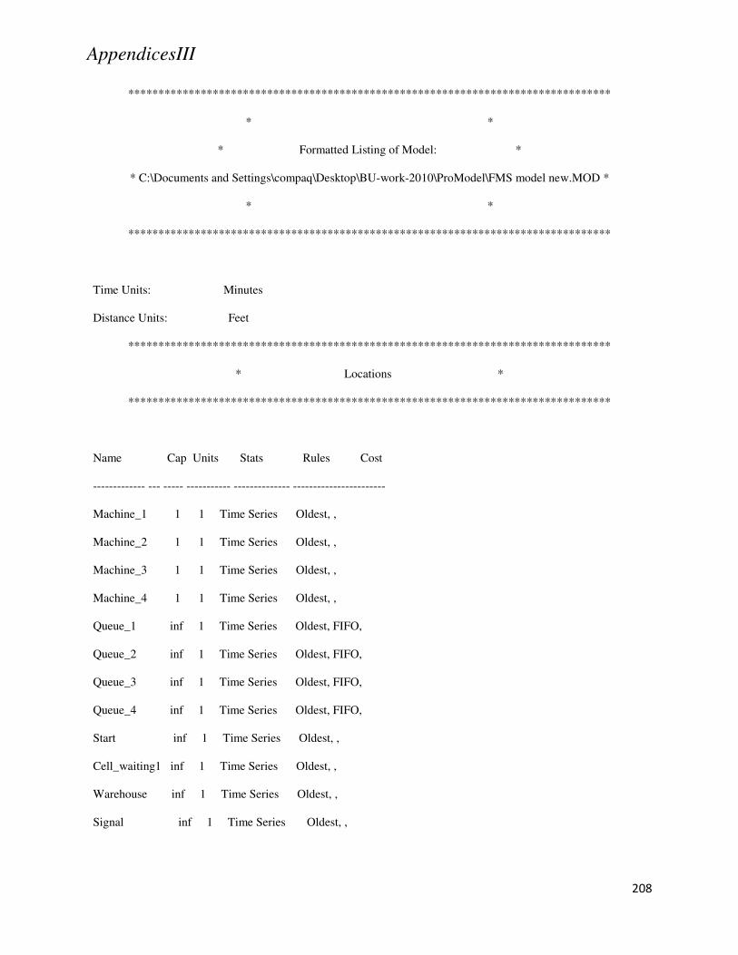
AppendicesIII
208
********************************************************************************
* *
* Formatted Listing of Model: *
* C:\Documents and Settings\compaq\Desktop\BU-work-2010\ProModel\FMS model new.MOD *
* *
********************************************************************************
Time Units: Minutes
Distance Units: Feet
********************************************************************************
* Locations *
********************************************************************************
Name Cap Units Stats Rules Cost
------------- --- ----- ----------- -------------- -----------------------
Machine_1 1 1 Time Series Oldest, ,
Machine_2 1 1 Time Series Oldest, ,
Machine_3 1 1 Time Series Oldest, ,
Machine_4 1 1 Time Series Oldest, ,
Queue_1 inf 1 Time Series Oldest, FIFO,
Queue_2 inf 1 Time Series Oldest, FIFO,
Queue_3 inf 1 Time Series Oldest, FIFO,
Queue_4 inf 1 Time Series Oldest, FIFO,
Start inf 1 Time Series Oldest, ,
Cell_waiting1 inf 1 Time Series Oldest, ,
Warehouse inf 1 Time Series Oldest, ,
Signal inf 1 Time Series Oldest, ,

AppendicesIII
209
********************************************************************************
* Usage downtimes for Locations *
********************************************************************************
Loc Frequency First Time Priority Logic
---------- ------------ ------------ ------------ ----------------------------
Machine_1 50 99 wait 15 min
Machine_2 90 99 wait 5 min
Machine_3 70 99 wait 10 min
Machine_4 80 99 wait 10 min
********************************************************************************
* Entities *
********************************************************************************
Name Speed (fpm) Stats Cost
------------- ------------ ----------- -------------------------
Product_1 150 Time Series
Product_2 150 Time Series
Product_3 150 Time Series
Product_4 150 Time Series
Product_dummy 150 Time Series

AppendicesIII
210
********************************************************************************
* Resources *
********************************************************************************
Res Ent
Name Units Stats Search Search Path Motion Cost
--------- ----- -------- ------ ------ ---------- -------------- -------------------------------------------
Operator1 1 By Unit None Oldest Empty: 150 fpm
Full: 150 fpm
Operator2 1 By Unit None Oldest Empty: 150 fpm
Full: 150 fpm
Operator3 1 By Unit None Oldest Empty: 150 fpm
Full: 150 fpm
Operator4 1 By Unit None Oldest Empty: 150 fpm
Full: 150 fpm
Operator5 1 By Unit None Oldest Empty: 150 fpm
Full: 150 fpm
Operator6 1 By Unit None Oldest Empty: 150 fpm
Full: 150 fpm
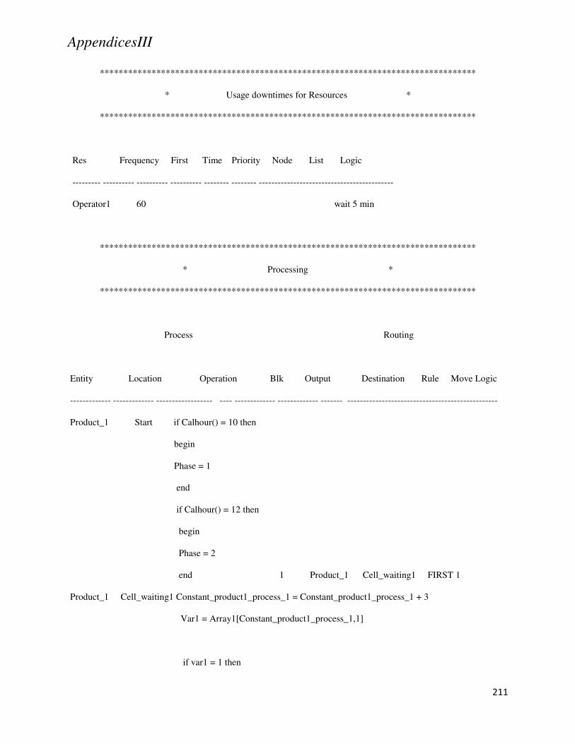
AppendicesIII
211
********************************************************************************
* Usage downtimes for Resources *
********************************************************************************
Res Frequency First Time Priority Node List Logic
--------- ---------- ---------- ---------- -------- -------- -------------------------------------------
Operator1 60 wait 5 min
********************************************************************************
* Processing *
********************************************************************************
Process Routing
Entity Location Operation Blk Output Destination Rule Move Logic
------------- ------------- ------------------ ---- ------------- ------------- ------- ------------------------------------------------
Product_1 Start if Calhour() = 10 then
begin
Phase = 1
end
if Calhour() = 12 then
begin
Phase = 2
end 1 Product_1 Cell_waiting1 FIRST 1
Product_1 Cell_waiting1 Constant_product1_process_1 = Constant_product1_process_1 + 3
Var1 = Array1[Constant_product1_process_1,1]
if var1 = 1 then

AppendicesIII
212
begin
Route 1
end
if var1 = 2 then
begin
Route 2
end 1 Product_1 Queue_1 FIRST 1
2 Product_1 Queue_4 FIRST 1
Product_1 Queue_1 1 Product_1 Machine_1 FIRST 1
Product_1 Machine_1 Constant_product1_process_2 = Constant_product1_process_2 + 3
Var2 = Array1[Constant_product1_process_2,1]
if Phase = 2 then
begin
use Operator5 for 10 min
end
if Phase = 1 then
begin
use Operator1 for 10 min
end
if Var2 = 1 then
begin
Route 1
end
if Var2 = 2 then
begin
Route 2
end 1 Product_1 Queue_2 FIRST 1
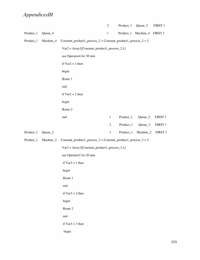
AppendicesIII
213
2 Product_1 Queue_3 FIRST 1
Product_1 Queue_4 1 Product_1 Machine_4 FIRST 1
Product_1 Machine_4 Constant_product1_process_2 = Constant_product1_process_2 + 3
Var2 = Array1[Constant_product1_process_2,1]
use Operator4 for 30 min
if Var2 = 1 then
begin
Route 1
end
if Var2 = 2 then
begin
Route 2
end 1 Product_1 Queue_2 FIRST 1
2 Product_1 Queue_3 FIRST 1
Product_1 Queue_2 1 Product_1 Machine_2 FIRST 1
Product_1 Machine_2 Constant_product1_process_3 = Constant_product1_process_3 + 3
Var3 = Array1[Constant_product1_process_3,1]
use Operator2 for 20 min
if Var3 = 1 then
begin
Route 1
end
if Var3 = 2 then
begin
Route 2
end
if Var3 = 3 then
begin

AppendicesIII
214
Route 3
end 1 Product_1 Queue_1 FIRST 1
2 Product_1 Queue_2 FIRST 1
3 Product_1 Queue_3 FIRST 1
Product_1 Queue_3 1 Product_1 Machine_3 FIRST 1
Product_1 Machine_3 Constant_product1_process_3 = Constant_product1_process_3 + 3
Var3 = Array1[Constant_product1_process_3,1]
if Phase = 2 then
begin
use Operator6 for 10 min
end
if Phase = 1 then
begin
use Operator3 for 10 min
end
if Var3 = 1 then
begin
Route 1
end
if Var3 = 2 then
begin
Route 2
end
if Var3 = 3 then
begin
Route 3
end 1 Product_1 Queue_1 FIRST 1
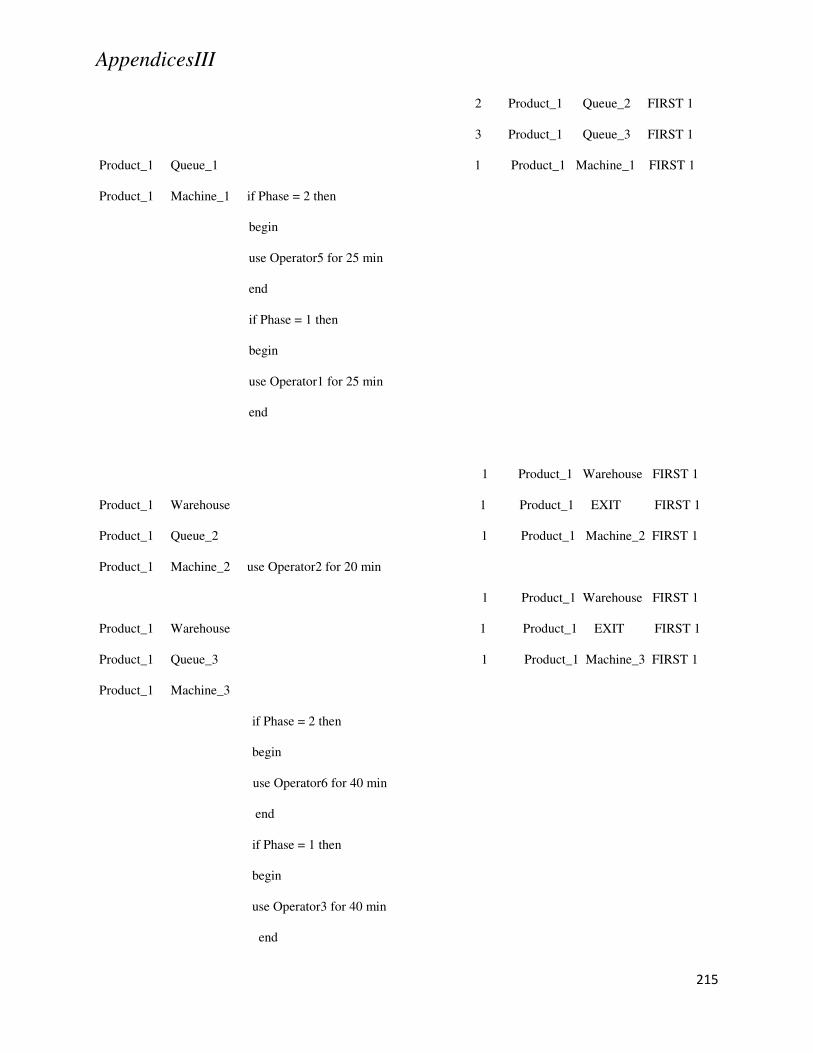
AppendicesIII
215
2 Product_1 Queue_2 FIRST 1
3 Product_1 Queue_3 FIRST 1
Product_1 Queue_1 1 Product_1 Machine_1 FIRST 1
Product_1 Machine_1 if Phase = 2 then
begin
use Operator5 for 25 min
end
if Phase = 1 then
begin
use Operator1 for 25 min
end
1 Product_1 Warehouse FIRST 1
Product_1 Warehouse 1 Product_1 EXIT FIRST 1
Product_1 Queue_2 1 Product_1 Machine_2 FIRST 1
Product_1 Machine_2 use Operator2 for 20 min
1 Product_1 Warehouse FIRST 1
Product_1 Warehouse 1 Product_1 EXIT FIRST 1
Product_1 Queue_3 1 Product_1 Machine_3 FIRST 1
Product_1 Machine_3
if Phase = 2 then
begin
use Operator6 for 40 min
end
if Phase = 1 then
begin
use Operator3 for 40 min
end
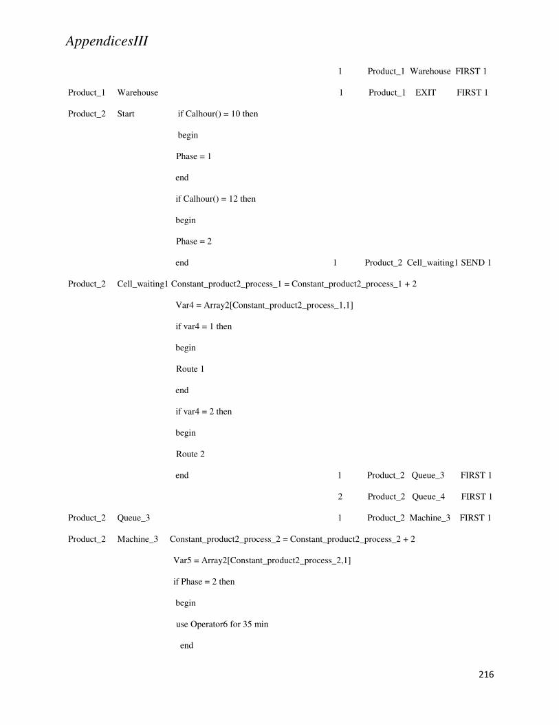
AppendicesIII
216
1 Product_1 Warehouse FIRST 1
Product_1 Warehouse 1 Product_1 EXIT FIRST 1
Product_2 Start if Calhour() = 10 then
begin
Phase = 1
end
if Calhour() = 12 then
begin
Phase = 2
end 1 Product_2 Cell_waiting1 SEND 1
Product_2 Cell_waiting1 Constant_product2_process_1 = Constant_product2_process_1 + 2
Var4 = Array2[Constant_product2_process_1,1]
if var4 = 1 then
begin
Route 1
end
if var4 = 2 then
begin
Route 2
end 1 Product_2 Queue_3 FIRST 1
2 Product_2 Queue_4 FIRST 1
Product_2 Queue_3 1 Product_2 Machine_3 FIRST 1
Product_2 Machine_3 Constant_product2_process_2 = Constant_product2_process_2 + 2
Var5 = Array2[Constant_product2_process_2,1]
if Phase = 2 then
begin
use Operator6 for 35 min
end
AppendicesIII
217
if Phase = 1 then
begin
use Operator3 for 35 min
end
if var5 = 1 then
begin
Route 1
end
if var5 = 2 then
begin
Route 2
end 1 Product_2 Queue_1 FIRST 1
2 Product_2 Queue_3 FIRST 1
Product_2 Queue_4 1 Product_2 Machine_4 FIRST 1
Product_2 Machine_4 Constant_product2_process_2 = Constant_product2_process_2 + 2
Var5 = Array2[Constant_product2_process_2,1]
use Operator4 for 25 min
if var5 = 1 then
begin
Route 1
end
if var5 = 2 then
begin
Route 2
end 1 Product_2 Queue_1 FIRST 1
2 Product_2 Queue_3 FIRST 1
Product_2 Queue_1 1 Product_2 Machine_1 FIRST 1
Product_2 Machine_1 if Phase = 2 then
AppendicesIII
218
begin
use Operator5 for 30 min
end
if Phase = 1 then
begin
use Operator1 for 30 min
end
1 Product_2 Warehouse FIRST 1
Product_2 Warehouse 1 Product_2 EXIT FIRST 1
Product_2 Queue_3 1 Product_2 Machine_3 FIRST 1
Product_2 Machine_3
if Phase = 2 then
begin
use Operator6 for 20 min
end
if Phase = 1 then
begin
use Operator3 for 20 min
end
1 Product_2 Warehouse FIRST 1
Product_2 Warehouse 1 Product_2 EXIT FIRST 1
Product_3 Start if Calhour() = 10 then
begin
Phase = 1
end
if Calhour() = 12 then
begin
Phase = 2
AppendicesIII
219
end 1 Product_3 Cell_waiting1 FIRST 1
Product_3 Cell_waiting1 Constant_product3_process_1 = Constant_product3_process_1 + 3
Var6 = Array3[Constant_product3_process_1,1]
if var6 = 1 then
begin
Route 1
end
if var6 = 2 then
begin
Route 2
end 1 Product_3 Queue_2 FIRST 1
2 Product_3 Queue_3 FIRST 1
Product_3 Queue_2 1 Product_3 Machine_2 FIRST 1
Product_3 Machine_2
Var7 = Array3[Constant_product3_process_2,1]
use Operator2 for 10 min
if var7 = 1 then
begin
Route 1
end
if var7 = 2 then
begin
Route 2
end 1 Product_3 Queue_1 FIRST 1
2 Product_3 Queue_4 FIRST 1
Product_3 Queue_3 1 Product_3 Machine_3 FIRST 1
Product_3 Machine_3
Var7 = Array3[Constant_product3_process_2,1]

AppendicesIII
220
if Phase = 2 then
begin
use Operator6 for 15 min
end
if Phase = 1 then
begin
use Operator3 for 15 min
end
if var7 = 1 then
begin
Route 1
end
if var7 = 2 then
begin
Route 2
end 1 Product_3 Queue_1 FIRST 1
2 Product_3 Queue_4 FIRST 1
Product_3 Queue_4 1 Product_3 Machine_4 FIRST 1
Product_3 Machine_4 Var8 = Array3[Constant_product3_process_3,1]
use Operator4 for 20 min
if var8 = 1 then
begin
Route 1
end
if var8 = 2 then
begin
Route 2
end 1 Product_3 Queue_2 FIRST 1
AppendicesIII
221
2 Product_3 Queue_4 FIRST 1
Product_3 Queue_1 1 Product_3 Machine_1 FIRST 1
Product_3 Machine_1
Var8 = Array3[Constant_product3_process_3,1]
if Phase = 2 then
begin
use Operator5 for 15 min
end
if Phase = 1 then
begin
use Operator1 for 15 min
end
if var8 = 1 then
begin
Route 1
end
if var8 = 2 then
begin
Route 2
end 1 Product_3 Queue_2 FIRST 1
2 Product_3 Queue_4 FIRST 1
Product_3 Queue_2 1 Product_3 Machine_2 FIRST 1
Product_3 Machine_2 use Operator2 for 20 min
1 Product_3 Warehouse FIRST 1
Product_3 Warehouse 1 Product_3 EXIT FIRST 1
Product_3 Queue_4 1 Product_3 Machine_4 FIRST 1
Product_3 Machine_4 use Operator4 for 15 min
1 Product_3 Warehouse FIRST 1

AppendicesIII
222
Product_3 Warehouse 1 Product_3 EXIT FIRST 1
Product_4 Start if Calhour() = 10 then
begin
Phase = 1
end
if Calhour() = 12 then
begin
Phase = 2
end 1 Product_4 Cell_waiting1 SEND 1
Product_4 Cell_waiting1 Constant_product4_process_1 = Constant_product4_process_1 + 2
Var9 = Array4[Constant_product4_process_1,1]
if Var9 = 1 then
begin
Route 1
end
if Var9 = 2 then
begin
Route 2
end
if Var9 = 3 then
begin
Route 3
end
if Var9 = 4 then
begin
Route 4
end 1 Product_4 Queue_1 FIRST 1
2 Product_4 Queue_2 FIRST 1
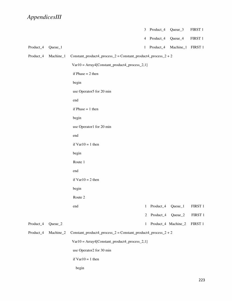
AppendicesIII
223
3 Product_4 Queue_3 FIRST 1
4 Product_4 Queue_4 FIRST 1
Product_4 Queue_1 1 Product_4 Machine_1 FIRST 1
Product_4 Machine_1 Constant_product4_process_2 = Constant_product4_process_2 + 2
Var10 = Array4[Constant_product4_process_2,1]
if Phase = 2 then
begin
use Operator5 for 20 min
end
if Phase = 1 then
begin
use Operator1 for 20 min
end
if Var10 = 1 then
begin
Route 1
end
if Var10 = 2 then
begin
Route 2
end 1 Product_4 Queue_1 FIRST 1
2 Product_4 Queue_2 FIRST 1
Product_4 Queue_2 1 Product_4 Machine_2 FIRST 1
Product_4 Machine_2 Constant_product4_process_2 = Constant_product4_process_2 + 2
Var10 = Array4[Constant_product4_process_2,1]
use Operator2 for 30 min
if Var10 = 1 then
begin

AppendicesIII
224
Route 1
end
if Var10 = 2 then
begin
Route 2
end 1 Product_4 Queue_1 FIRST 1
2 Product_4 Queue_2 FIRST 1
Product_4 Queue_3 1 Product_4 Machine_3 FIRST 1
Product_4 Machine_3 Constant_product4_process_2 = Constant_product4_process_2 + 2
Var10 = Array4[Constant_product4_process_2,1]
if Phase = 2 then
begin
use Operator6 for 10 min
end
if Phase = 1 then
begin
use Operator3 for 10 min
end
if Var10 = 1 then
begin
Route 1
end
if Var10 = 2 then
begin
Route 2
end 1 Product_4 Queue_1 FIRST 1
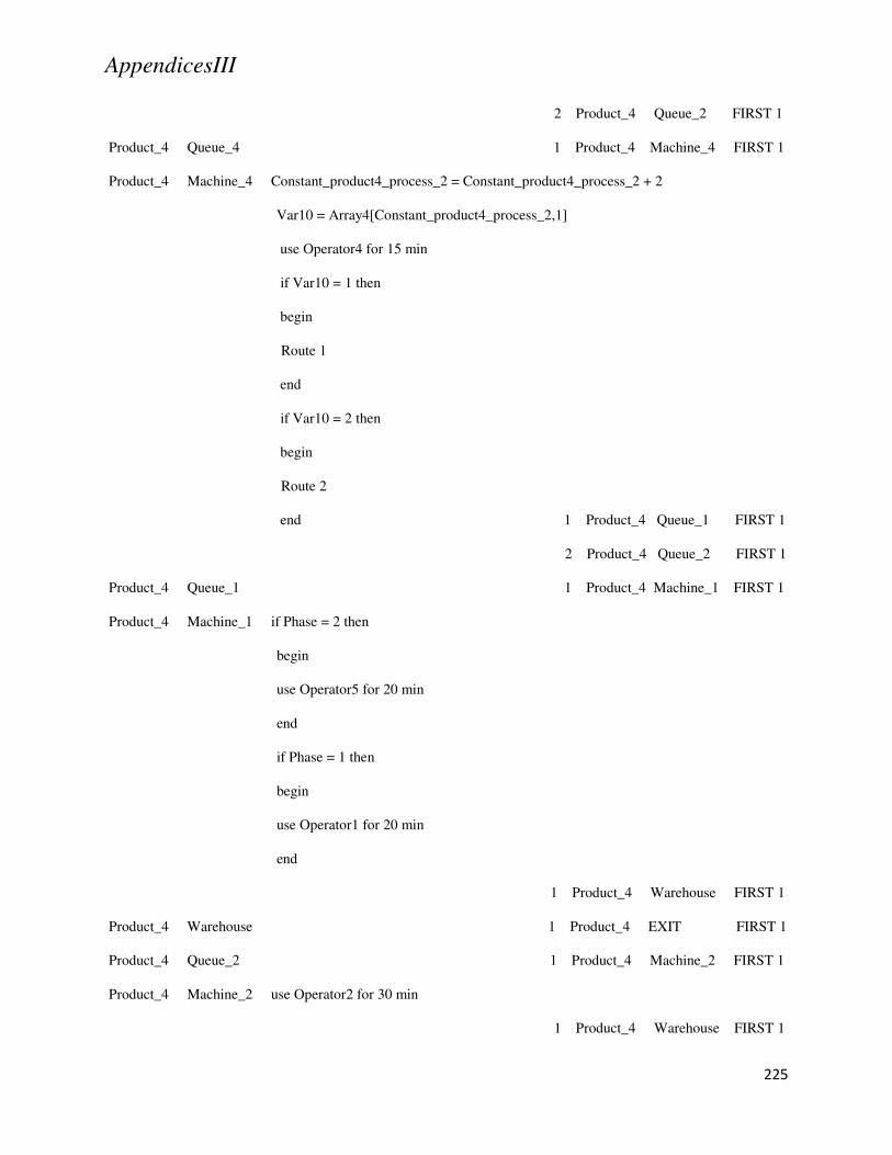
AppendicesIII
225
2 Product_4 Queue_2 FIRST 1
Product_4 Queue_4 1 Product_4 Machine_4 FIRST 1
Product_4 Machine_4 Constant_product4_process_2 = Constant_product4_process_2 + 2
Var10 = Array4[Constant_product4_process_2,1]
use Operator4 for 15 min
if Var10 = 1 then
begin
Route 1
end
if Var10 = 2 then
begin
Route 2
end 1 Product_4 Queue_1 FIRST 1
2 Product_4 Queue_2 FIRST 1
Product_4 Queue_1 1 Product_4 Machine_1 FIRST 1
Product_4 Machine_1 if Phase = 2 then
begin
use Operator5 for 20 min
end
if Phase = 1 then
begin
use Operator1 for 20 min
end
1 Product_4 Warehouse FIRST 1
Product_4 Warehouse 1 Product_4 EXIT FIRST 1
Product_4 Queue_2 1 Product_4 Machine_2 FIRST 1
Product_4 Machine_2 use Operator2 for 30 min
1 Product_4 Warehouse FIRST 1
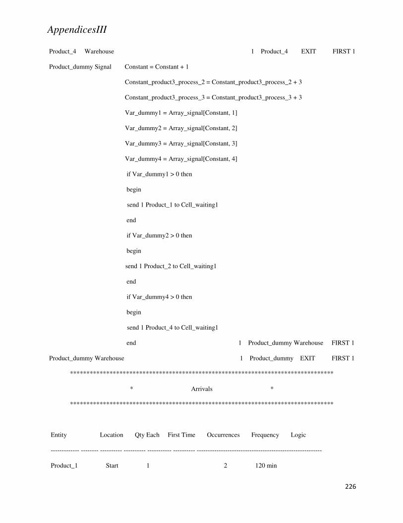
AppendicesIII
226
Product_4 Warehouse 1 Product_4 EXIT FIRST 1
Product_dummy Signal Constant = Constant + 1
Constant_product3_process_2 = Constant_product3_process_2 + 3
Constant_product3_process_3 = Constant_product3_process_3 + 3
Var_dummy1 = Array_signal[Constant, 1]
Var_dummy2 = Array_signal[Constant, 2]
Var_dummy3 = Array_signal[Constant, 3]
Var_dummy4 = Array_signal[Constant, 4]
if Var_dummy1 > 0 then
begin
send 1 Product_1 to Cell_waiting1
end
if Var_dummy2 > 0 then
begin
send 1 Product_2 to Cell_waiting1
end
if Var_dummy4 > 0 then
begin
send 1 Product_4 to Cell_waiting1
end 1 Product_dummy Warehouse FIRST 1
Product_dummy Warehouse 1 Product_dummy EXIT FIRST 1
********************************************************************************
* Arrivals *
********************************************************************************
Entity Location Qty Each First Time Occurrences Frequency Logic
------------- -------- ---------- ---------- ----------- ---------- ---------------------------------------------------------
Product_1 Start 1 2 120 min
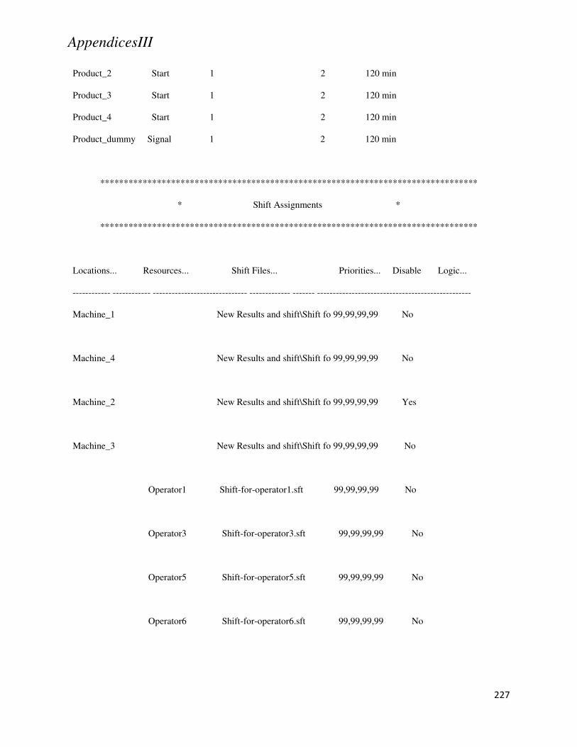
AppendicesIII
227
Product_2 Start 1 2 120 min
Product_3 Start 1 2 120 min
Product_4 Start 1 2 120 min
Product_dummy Signal 1 2 120 min
********************************************************************************
* Shift Assignments *
********************************************************************************
Locations... Resources... Shift Files... Priorities... Disable Logic...
------------ ------------ ------------------------------ ------------- ------- -------------------------------------------------
Machine_1 New Results and shift\Shift fo 99,99,99,99 No
Machine_4 New Results and shift\Shift fo 99,99,99,99 No
Machine_2 New Results and shift\Shift fo 99,99,99,99 Yes
Machine_3 New Results and shift\Shift fo 99,99,99,99 No
Operator1 Shift-for-operator1.sft 99,99,99,99 No
Operator3 Shift-for-operator3.sft 99,99,99,99 No
Operator5 Shift-for-operator5.sft 99,99,99,99 No
Operator6 Shift-for-operator6.sft 99,99,99,99 No
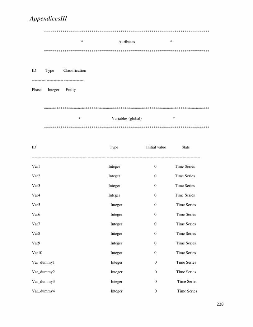
AppendicesIII
228
********************************************************************************
* Attributes *
********************************************************************************
ID Type Classification
---------- ------------ --------------
Phase Integer Entity
********************************************************************************
* Variables (global) *
********************************************************************************
ID Type Initial value Stats
--------------------------- ------------ ------------- --------------------------------------------------------------------
Var1 Integer 0 Time Series
Var2 Integer 0 Time Series
Var3 Integer 0 Time Series
Var4 Integer 0 Time Series
Var5 Integer 0 Time Series
Var6 Integer 0 Time Series
Var7 Integer 0 Time Series
Var8 Integer 0 Time Series
Var9 Integer 0 Time Series
Var10 Integer 0 Time Series
Var_dummy1 Integer 0 Time Series
Var_dummy2 Integer 0 Time Series
Var_dummy3 Integer 0 Time Series
Var_dummy4 Integer 0 Time Series
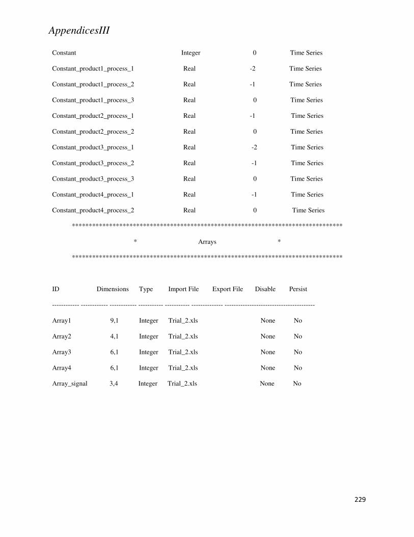
AppendicesIII
229
Constant Integer 0 Time Series
Constant_product1_process_1 Real -2 Time Series
Constant_product1_process_2 Real -1 Time Series
Constant_product1_process_3 Real 0 Time Series
Constant_product2_process_1 Real -1 Time Series
Constant_product2_process_2 Real 0 Time Series
Constant_product3_process_1 Real -2 Time Series
Constant_product3_process_2 Real -1 Time Series
Constant_product3_process_3 Real 0 Time Series
Constant_product4_process_1 Real -1 Time Series
Constant_product4_process_2 Real 0 Time Series
********************************************************************************
* Arrays *
********************************************************************************
ID Dimensions Type Import File Export File Disable Persist
------------ ------------ ------------ ----------- ----------- -------------- ----------------------------------------
Array1 9,1 Integer Trial_2.xls None No
Array2 4,1 Integer Trial_2.xls None No
Array3 6,1 Integer Trial_2.xls None No
Array4 6,1 Integer Trial_2.xls None No
Array_signal 3,4 Integer Trial_2.xls None No

AppendicesIII
230
********************************************************************************
* External Files *
********************************************************************************
ID Type File Name Prompt
---------- ----------------- ------------------------------------------- -------------------------------------------
(null) Trial_2.xls
(null) Shift Shift-for-operator3.sft
(null) Shift Shift-for-operator6.sft
(null) Shift Shift-for-operator1.sft
(null) Shift Shift-for-operator5.sft
(null) Shift New Results and shift\Shift for mc2 sc5.sft
(null) Shift New Results and shift\Shift for mc1 sc1.sft
(null) Shift New Results and shift\Shift for mc4 sc1.sft
(null) Shift New Results and shift\Shift for mc3 sc1.sft