Embed Size (px)
Citation preview
Lookup Table’s Functionality within Color Spaces and Motion Picture
J O N A T H A N F R A N S S O N
Bachelor of Science Thesis Stockholm, Sweden 2008

Lookup Table’s Functionality within Color Spaces and Motion Picture
J O N A T H A N F R A N S S O N
Bachelor’s Thesis in Media Technology (15 ECTS credits) at the Degree Programme in Media Technology Royal Institute of Technology year 2008 Supervisor at CSC was Björn Hedin Examiner was Roger Wallis TRITA-CSC-E 2008:080 ISRN-KTH/CSC/E--08/080--SE ISSN-1653-5715 Royal Institute of Technology School of Computer Science and Communication KTH CSC SE-100 44 Stockholm, Sweden URL: www.csc.kth.se

Lookup Table’s functionality within color spaces
and motion picture
Abstract
In the motion picture industry of post production, Lookup Tables are used partly for
time efficiency. A Lookup Table works as lay about for color editing, but is also a
converter between linear and logarithmic color definition. The Lookup Tables for
motion picture are working in three dimensions, width, height and deep. There are
different industry standards for Lookup Tables, where the Kodak standard is
considered as a world leading technology.
With the possibility of editing Lookup Tables, the line of production will be more
efficient. Predefined Lookup Tables don’t have to be remade if a small change is
necessary, and with the knowledge of the underlying algorithms, several Lookup
Tables can be merged into one. This is beneficial, since the project has to be rendered
before a second Lookup Table can be applied. The time of rendering can sometimes,
even with modern high capacity computers, be considerable.
This project has provided such a Lookup Table editor, and its accuracy has been
evaluated. For the production of this software, advanced mathematics combined with
knowledge in colorimetric, programming and common computer science have been
required. With the combination of these areas, the knowledge in how the Kodak
algorithms are formed could be obtained.
When the analysis of Kodak standard was complete, and the software was produced,
an evaluation for its functionality was made. Most of the software’s image editing
options, such as increasing or decreasing Brightness, Bright regions, Contrast and
Color Balance, are working well enough for industry standards. The option
Saturation is however today not working with the desired accuracy, and it needs to be
further explored for fulfilling industry standards.

Lookup Tables funktion i färgrymder och rörlig
bild
Sammanfattning
Lookup Tables används bland annat i produktionen för rörlig bild för att effektivisera
produktionsflödet. En Lookup Table kan bektraktas som en lathund för
färgkorrigering, men används även som konverterare mellan linjär och logaritmisk
färgdefinition. Lookup Tables som används inom rörlig bild arbetar i de tre
dimensionerna bredd, höjd och djup. På marknaden finns ett flertal standarder för
Lookup Tables, varav Kodak är ansett som världsledande.
Med möjligheten att kunna redigera Lookup Tables så effektivseras produktionflödet,
eftersom det inte längre är nödvändigt att skapa en helt ny Lookup Table när
ändringar är önskade. Att känna till hur pixelvärdena förändras vid bildbehandlingen
resulterar i att flera Lookup Tables kan bli sammanfogade till en. Detta har stort
användningsvärde i renderingsprocessen, eftersom endast en Lookup Table kan åt
gången vara applicerad. Det innebär att renderingstiden blir förkortad till bråkdelar av
ordinarie tid, vilket är av stor fördel eftersom tiden det tar att rendera ett projekt kan,
även med dagens datorkapacitet, vara avsevärd.
Detta projekt har producerat en sådan mjukvara för korrigering av Lookup Tables,
och den har blivit utvärderad huruvida den uppfyller industrins krav. I arbetat har
avancerad matematik kombinerat med kunskaper i kolorimetri, programmering och
allmän datorvetenskap använts. Med behärskning av dessa områden kunde Kodaks
processer för färghantering kartläggas.
När programmet var klart kunde en omfattande utvärdering göras, som visade hur bra
programmet fungerar. De flesta av de olika verktygen för färghantering, såsom att öka
eller att minska hela bildens ljusstyrka, delar av bildens ljusstyrka, kontrast och
färgbalans fungerar tillräckligt bra för att användas i kommersiellt bruk. Verktyget att
öka eller att minska bildens färgmättnad är dock i dag inte tillräckligt välfungerande
för att uppfylla industrins krav.

Preface
This thesis is for Bachelor degree in Media Technology, and has been done for the
School of Computer Science and Communications (CSC), at the Royal Institute of
Technology, known as KTH, in Stockholm, Sweden. My job requestor is The
Chimney Pot, which delivers post production services for motion picture. Their
projects are often commercials, short movies and full length movies. The Chimney
Pot has offices Europe around, and the main job requestor has been the office in
Warsaw, Poland.
I would like to thank my main tutor, Björn Hedin, Lecturer at CSC, KTH, for his
efforts in helping me with my work of academic nature and for proofreading this
report. I would also like to thank my instructors Christer Lie, Lecturer at CSC, KTH,
for giving me help concerning colorimetric and Kamil Rutkowski, Digital
Intermediate at The Chimney Pot, for assisting me with my project and educating me
in common computer science.
Special thanks to
Jens Fransson, Docent at School of Engineering Science, KTH, for being my mentor
and frequently been helping me with my academic work for the past years.
Jonathan Fransson
Stockholm, Sweden. June 2008

Tables of contents 1 INTRODUCTION ...................................................................................................................1
1.1 Background .....................................................................................................................1
1.2 Purpose ............................................................................................................................2
1.3 Goal..................................................................................................................................3
1.4 Research questions.........................................................................................................3
2 METHOD...............................................................................................................................5
2.1 Deciding program language.........................................................................................5
2.2 Measuring pixel values...................................................................................................5
2.3 Analyzing measured data..............................................................................................6
2.4 Implementing the approximations ................................................................................7
2.4 Evaluating the results ......................................................................................................7
3 BACKGROUND AND THEORY .............................................................................................8
3.1 RGB and HSB color spaces.............................................................................................8
3.2 Color in bits ....................................................................................................................10
3.3 Logarithmic color definition .........................................................................................10
4 RESULTS ..............................................................................................................................12
4.1 Program language and operating systems................................................................12
4.2 DPX patches ..................................................................................................................12
4.3 Analysis of measured pixel values ..............................................................................13
4.3.1 Brightness ....................................................................................................................13
4.3.2 Contrast.......................................................................................................................15
4.3.3 Bright regions..............................................................................................................18
4.3.4 Saturation....................................................................................................................20
4.3.5 Balance.......................................................................................................................27

5 EVALUATION......................................................................................................................31
5.1 Brightness and Contrast ................................................................................................31
5.2 Bright regions .................................................................................................................33
5.3 Saturation.......................................................................................................................35
5.4 Balance..........................................................................................................................36
6 CONCLUSIONS..................................................................................................................38
7 FUTURE RESEARCH.............................................................................................................39
8 REFERENCES.......................................................................................................................40
8.1 Books..............................................................................................................................40
8.2 Webb..............................................................................................................................40
9 APPENDICES ......................................................................................................................41
9.1 Analysis of hexadecimal machinery code ................................................................41
9.2 Algorithm for conversion between color spaces .......................................................41
9.3 Saturation anamolies ....................................................................................................42
10 GLOSSARY.......................................................................................................................44

Introduction ___________________________________________________________________________
- 1 -
1 Introduction
1.1 Background In a late phase of producing motion picture, the picture’s appearance is modified.
This is done because colors convey a message, even if other parts of a video are more
important, like ambience sound, music and dialogs. It is however important that the
colors go together with the rest of the emotional stimulus. As if the message is that
the temperature in the picture is low, often the blue channel is brought up, to give a
cold experience. Another example is when the desired shooting conditions aren’t
available. The lost visual affects that provides, can sometimes be emulated
afterwards, by color editing.
There are different operations in color correcting a picture. It can be brightened or
darkened, and its contrast can be increased or decreased. Another example is the
Color balance, which is a powerful tool where specific areas of the picture can be
brought more of a certain color.
The basic idea of color correction is to work on pixel level. When editing a motion
picture, directly scanned from film negative without any compression, each pixel for
each frame will be run through an advanced mathematical operation. To speed the
production up, a Lookup Table (LUT) can be applied. It holds color editing
information, and is also working with an interpolation technique. In the LUT there are
some predefined pixel values formed as a list, where each ingoing pixel value can be
looked up to find its corresponding output. If there isn’t a predefined output value for
the input, the resulted pixel value is estimated by its closest neighbors.
LUTs are useful in many scientific fields, and in media production they can be
considered as layabouts for color corrections (Green, 1999). LUTs are used when the
final color editing takes place, but also sooner in the line of production, as in when
the film negative is scanned. There are several LUTs with different properties and
standards, produced by companies around the world. Kodak is such a company,
which standard is considered as world leading, and it’s the standard this project will
focus on. The different LUTs are applied depending on the desired picture attributes,

Introduction ___________________________________________________________________________
- 2 -
and the colors can later be finely adjusted. Only one LUT can be applied at time,
since the LUT often is chosen in connection with opening, or creating, a new project
in the video editing software. An example of such software is the Nucoda SD/HD,
provided by Digital Vision (Digital Vision).
LUTs are also needed for certain conversions, such as the conversion between
logarithmic and linear color definition (Chapter 3.3). Different systems work either
linearly or logarithmical, and when these systems meet, a LUT will sustain the color
perception of the motion picture.
When a LUT is applied to a project, advanced mathematics is calculating pixel values
for handling color data. The LUT is, simply explained, a carrier for certain directions
that calls the video software to manipulate with the picture’s appearance. In such way,
the desired change is obtained. It is not hard to see, that the LUTs are an essential part
in the line of production for motion picture.
There is software for creating Lookup Tables which are working in three dimensions
with pixel width, pixel height and time line. But the possibilities of editing a
predefined LUT are limited, because no well established software with such an option
exists.
1.2 Purpose
Even if there are several predefined LUTs to select from, very often a slight change of
the LUTs color directions would be beneficial. Sometimes it is desired to color
correct the LUT directly, instead of making the specific corrections when the finely
adjustment is performed. Certain LUTs are used more often than others for the same
customers, which will bring the human editor to repeat his manual operations. Such a
desired correction can for example be to make the shadows more bluish.
Sometimes there is a need to apply several LUTs to accomplish the desired visual
affect. However the application of a LUT is fast, the entire project has to be rendered
before a second LUT can be applied. With the knowledge of approximated algorithms
for LUT functions, the time of production can remarkably be shortened. With the
possibility to merge two LUTs into one, the rendering time can be reduced by half

Introduction ___________________________________________________________________________
- 3 -
time in the situations where two LUTs are needed. This is a given result, because the
project only needs to be rendered once.
To be able to edit, and merge, three dimensional LUTs, a separated program with a
user interface is required. It is impossible to manually edit a LUT, since the
underlying mathematics is not easily embraced. To obtain such possibility, a technical
investigation is required, since Kodak won’t very likely hand out their unofficial
methods of color editing. When the approximations are found, the line of further
possibilities takes place.
1.3 Goal The main goal for this project is to create a well working LUT editor. This editor will
be considered as a tool for increased effectiveness in post production of motion
picture. The part goal is to analyze how color handling of Kodak standard is
behaving, and making approximated functions for emulation. A future goal is, by
knowing the algorithms of color editing, adding the color affect of several LUTs to
one single LUT.
1.4 Research questions
The following question formulations need to be answered for achieving above goals.
• How do the LUTs of Kodak standard precisely affect the pixel values of the
picture? (Main question)
• How can the Kodak standard algorithms for image processing be
approximated for the best emulated performance?
• Can the produced approximations be accurate enough for industry standards?
• In which programming language should such software be written?
To know how the LUTs are affecting the pixel values is the basis for an approach of
producing software for LUT editing. It will be explored by analyzing a series of
measurements of Kodak standard, where the second research question will be
processed: How the algorithms can be approximated?

Introduction ___________________________________________________________________________
- 4 -
Before releasing the program for commercial use, it is significant that it’s fulfilling
the industry standards. To simplify this decision, the accuracy of the approximations
will show in a solid evaluation.

Method ___________________________________________________________________________
- 5 -
2 Method This project was about producing a program from scratch, and every part of the way
to the final product. Since this work was done by, more or less, one person, it was
planned to take about six months. This chapter will give an overall picture of how the
research questions were approached.
2.1 Deciding program language The program language should be set in an early phase. Since this project was about a
new kind of software, it was significant to consider the different possibilities. The
program must run steadily, and be able to do large amount of advanced calculations.
It is also important that the program is easily accessible, why an online solution was
considered
2.2 Measuring pixel values To obtain the knowledge of the Kodak standard for LUTs, the access to a video
editing system, that is Kodak certified, was required. Digital vision provides such a
system, called Nucoda HD/SD, which is the equipment The Chimney Pot is using.
The basic idea of retrieving an understanding of the LUT’s underlying mathematics
was to collect data for analysis. To obtain this data, the affect of color editing options
had to somehow be measured. By comparing images, before and after they were
edited, a foundation for the perceptual behavior was set. The comparison was
accurately done by measuring the pixel values of the ‘before’ and ‘after’ images.
It required several steps to get hold of the pixel values. It wasn’t as simple as opening
the image in a text editor, since the machine code contains other information than the
pixel values, like the dimensions of the image and Meta data. The machine code was
expressed in hexadecimals, where the highest possible value is FFFF, or in decimals, 162 . The flow of information in the machine code was divided in hexadecimal way, as
in: “802A 5FD7 0000 0800…”. Since the original pixel values were expressed in

Method ___________________________________________________________________________
- 6 -
10bits, and every part of the machine code is expressed in 2bytes, an accommodation
was necessary to access the information and saving it to a text file (Chapter 9.1).
With the Nucoda, several patches of exported images were made. When opening a
certain image, it could be exported into a new image file with the applied affects that
was currently set. This was done several times for each kind of image editing option,
such as Brightness, Contrast, Saturation, Color Balance and Bright Regions. Each
option was used 20 times for creating enough patches, where each patch was an
increase or decrease by 10%.
The image that would be used for creating the patches had to carefully be composed.
The image’s properties, in both dimensions and appearance, had to be representative
for the analysis. Also the file type was a matter under discussion, since no data loss is
desired when the image is exported.
2.3 Analyzing measured data The measured pixel data was imported to Microsoft Excel for analysis. In Excel, a
first impression of the pixel behavior was given, by simply plotting the input and
output data. Sometimes an approximated function became trivial as the plotted graph
appeared, other times further analysis was required for understanding the link
between input and output data. Research in colorimetric and mathematics was done to
reach the goal of computing mathematical functions for emulating the LUT’s
algorithms.
Sometimes when the input/output relations were unclear, the data was differently
sorted in the pursuit to see any links. It was successful, and for sorting this amount of
data, small methods were programmed in Java. In this way, the pixel behavior for the
Saturation option was further explored.
Microsoft Excel is an easy tool for analysis, and was the mostly used software during
this project, but it was shown later on that the Excel’s tool Add Trend Line wasn’t
always accurate enough. Whenever the tests of the provided functions from Excel
didn’t give the expected results, the mathematical program MatLab was used. MatLab
is in some ways more difficult to handle but is in every way a more powerful

Method ___________________________________________________________________________
- 7 -
mathematical tool than Excel. From a perspective of time, Excel was chosen to be the
main software for the analysis, and whenever needed, MatLab could compensate for
the weaknesses of Excel.
2.4 Implementing the approximations The analysis resulted in functions for calculation of output pixel values. All of the
above mentioned color editing options were approximated, and then implemented in a
version of the software without a user interface. Every function was rapidly checked
in connection with the implementation, because it was convenient to be sure of no
logical errors had occurred.
2.4 Evaluating the results The evaluation had its purpose to give a notification how well the software actually
works as a LUT editor. It was wise to know how close the calculated pixel values
were to the measured ones, before using the software commercially.
In the new software, the same patches as earlier created in the Nucoda system were
remade. These patches could be compared to the ones used for analysis, and it was
easy to see the differences when imported to Excel. Additional patches were created
when the current option was set to factors between 10 and 20%. Since all of the
patches were made in an increased, or decreased, level of 10%, it was wise to check if
the estimated output values were reasonable.
When comparing the Nucoda patches to the new patches, three values were
interesting. They were the biggest positive and negative anomalies, which gives an
impression of how bad the function’s outputs possibly could be. But to give a full
perspective in the accuracy of the LUT editor, the two above values together with the
average anomaly were required. These three values, together with advisement from
The Chimney Pot, gave a solid evaluation if the LUT editor was working well enough
for commercial use.

Background and theory ___________________________________________________________________________
- 8 -
3 Background and theory
In this chapter, some of the underlying theories for this project are presented. Since
this project has been about computer science and colorimetric, color spaces and
digital color definition will be discussed. The basics of the areas can be read here,
and for the interested, the referred literature is for further reading.
3.1 RGB and HSB color spaces
Working with digital colors means that somehow the colors are needed to be
expressed with numbers or digits. To do so several color spaces have been created
and today there are a numerous of them. To shortly explain what a color space is, one
can say it is a three dimensional chart with axes that are numbered by some kind of
scale.
Color spaces are being used depending on the situation, if the product is something
printed, a motion picture, or for web, etc.
Many have heard about ‘RGB’ in some kind of context, mostly because it is the most
well known color space. The name RGB is an abbreviation for red, green and blue,
and it is these colors the RGB color space is using to define every color in this space
(Fig 3.1). These three colors are also known as the primary colors, because together
they can define every possible color there is.
The RGB color space has the form of a cube, where three of the corners are the
primary colors (Gonzalez and Woods, 2008). The other five corners
are white, black and the complementary colors cyan, magenta
and yellow, which all are a mixture of two, or of all three, of
the primary colors. To define one color in RGB the coordinates
of a vector is used. For instance is [255, 0, 0] red, [0, 255, 0] is
green, [0, 0, 255] is blue, [0, 0, 0] is black and [255, 255, 255] Fig 3.1 RGB color space

Background and theory ___________________________________________________________________________
- 9 -
is white. The complementary colors cyan, magenta and yellow have the values [0,
255, 255], [255, 0, 255] and [255, 255, 0]. These colors are expressed in 8 bits which
is further explained in Chapter 3.2.
Another less common color space is the HSB (Fig 3.2). This color space defines colors
in, what usually is perceived as, a more understandable way. The three axes are hue,
saturation and brightness, and here all three expressions are being explained.
Hue is, according to the CIE, ‘the attribute of a visual sensation according to which
an area appears to be similar to one of the perceived colors, red, yellow, green and
blue, or a combination of the two of them’ (Poynton). Hue is what a layman would call
‘shade’ or perhaps even ‘color’. In the HSB color space, hue is scaled in degrees,
from 0 to 360, where 0 degrees is red, 120 degrees is green and 240 degrees is blue.
Between these values of hue one can find the complementary colors cyan, magenta
and yellow, having the respective hues at 180, 300 and 60 degrees. The hue scaling is
formed as a circle.
Saturation is, again according to the CIE, “the colorfulness of an area judged in
proportion to its brightness” (Poynton). The hue runs from neutral gray to fully
saturated color, and this is scaled in level of percentage in the HSB color space. The
saturation axis runs at the chosen direction of the hue.
Brightness should be the most understandable expression of these three, and in the
HSB color space it is simply how bright the colors appear. The brightness is, as the
saturation, scaled in level of percentage and runs up and
down along what could be seen as a normal vector to the
laying circle of the hue scaling. Together with the scaling of
hue and saturation a cone is perceived when approaching a
chart of the HSB color space.
Fig 3.2 HSB color space

Background and theory ___________________________________________________________________________
- 10 -
3.2 Color in bits
When an image is digitized it is always in some way divided into many smaller
pieces, called pixels. Each pixel describes precisely one color with a numerical value.
For instance, in the RGB color space, each color is defined by a mix of the three
primary colors red, green and blue (Chapter 3.1).
Digital colors are defined in bits, and the more bits that are being used the more
accurate approximation of a single color’s value will be provided. When working
with several pixels, as in an image, there is a way to make the bits last longer (Chapter
3.3).
In many systems 8bits are being used, which is very convenient since 8bits founds 1
byte, and the highest value is therefore [11111111] in binary system and 255 in
decimal system (Watkinson, 2001). In the Nucoda system however, the colors are being
defined in 10bits depth, which can cause problems whenever expressing the values in
bytes is desired, since (10 ⋅n) mod 8 ≠ 0.
3.3 Logarithmic color definition
The values of an image can be declared either linearly or logarithmically. In a linear
system, each input value has its corresponded output value in a linear expression.
What this means practically is easier to describe as in an example from a common
situation.
A monitor, for computer or television, is working linearly. When the picture is too
dark, it can most often be brightened by pressing the gain button on the screen. When
the button is pressed, each level of increased voltage in the monitors signal, results in
an equally amount of increased brightness on the screen.
A typical system which is working logarithmically is the old fashioned film camera
which has well defined capturing in the dark and light areas. It can be described as the
silver ions on the film are not equally divided for the shadows/highlights and
midtones, they are logarithmically divided.

Background and theory ___________________________________________________________________________
- 11 -
When working linearly, shadows, midtones and highlights have an equally dedicated
space for data storage. In a logarithmical environment the bits are spread and as a
result there will be more dedicated space storage for the information in the shadows
and highlights, as illustrated in Graph 3.1 (Gonzalez and Woods, 2008).
This gives an image with more details in the darker and lighter areas. The price for
this benefit is the reduced data from the midtones, which is highly acceptable since
the shadows, and highlights, requires more data than the midtones to obtain the same
perception. In the graph below a diagram shows the difference between a linear curve
(blue) and a logarithmic curve (red). In the shadows, the red curve is taking a longer
way than the blue curve to enter the area of midtones. If the bits on the two different
curves appear regularly, it is trivial that the logarithmic curve has a better data storage
capacity in the shadows, than the linear curve. The same reasoning is appliable for the
curves in the highlights tone.
Graph 2.1
Results ___________________________________________________________________________
- 12 -
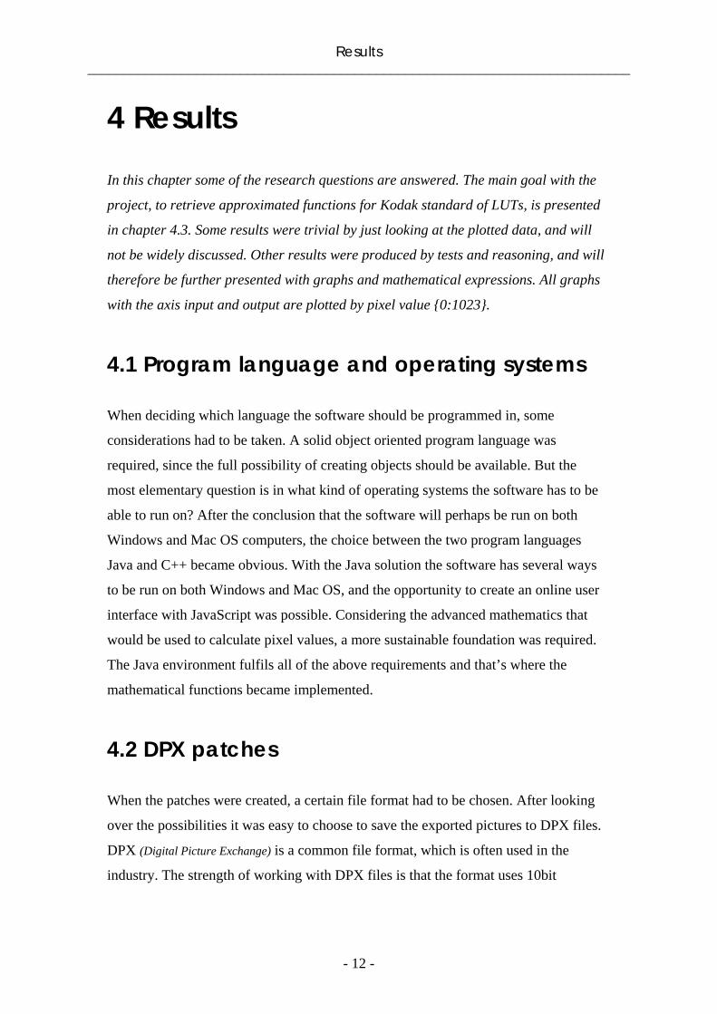
4 Results
In this chapter some of the research questions are answered. The main goal with the
project, to retrieve approximated functions for Kodak standard of LUTs, is presented
in chapter 4.3. Some results were trivial by just looking at the plotted data, and will
not be widely discussed. Other results were produced by tests and reasoning, and will
therefore be further presented with graphs and mathematical expressions. All graphs
with the axis input and output are plotted by pixel value {0:1023}.
4.1 Program language and operating systems
When deciding which language the software should be programmed in, some
considerations had to be taken. A solid object oriented program language was
required, since the full possibility of creating objects should be available. But the
most elementary question is in what kind of operating systems the software has to be
able to run on? After the conclusion that the software will perhaps be run on both
Windows and Mac OS computers, the choice between the two program languages
Java and C++ became obvious. With the Java solution the software has several ways
to be run on both Windows and Mac OS, and the opportunity to create an online user
interface with JavaScript was possible. Considering the advanced mathematics that
would be used to calculate pixel values, a more sustainable foundation was required.
The Java environment fulfils all of the above requirements and that’s where the
mathematical functions became implemented.
4.2 DPX patches
When the patches were created, a certain file format had to be chosen. After looking
over the possibilities it was easy to choose to save the exported pictures to DPX files.
DPX (Digital Picture Exchange) is a common file format, which is often used in the
industry. The strength of working with DPX files is that the format uses 10bit

Results ___________________________________________________________________________
- 13 -
logarithmic color definition, and can therefore maintain the exported data without any
loss of accuracy of the pixel values.
The original DPX file should have the same properties as a LUT, and it is significant
that the inbuilt color management of the system does not affect the picture in any
way. If it does, the exported images will contain pixel information from the precise
settings of the current system, and the software will be based on the exact same
circumstances. As already declared, any LUT’s purpose is to affect the picture, and a
LUT with the purpose of leaving the picture the way it originally was, sounds in
every case needless. In this case however, such LUT is not entirely unnecessary.
To be certain that nothing else but the intentional image editing is affecting the
picture during this measurement, a DPX file representation of LUT that makes no
changes should be used. In this way the exported images will be entirely free from
any kind of affects than the purposive ones. Therefore, the DPX image file will have
the same dimensions as the LUTs, i.e. 17 × 289 pixels. This image has well defined
shadows, midtones and highlights in all of the primary and complementary colors,
and works fine as a starting-point for researching the behaviors of the pixel values
(Fig 4.1). Such a LUT, and the technique of converting DPX image files into simple
text files, back and forth, was provided by Kamil Rutkowski at The Chimney Pot.
4.3 Analysis of measured pixel values
4.3.1 Brightness
The mathematical meaning of increased brightness is that all the pixels will have their
values increased. If it is desired to lift the entire image, such as shadows, midtones
and highlights, all of the pixels will be affected the same way. It was confirmed, when
going through the measured pixels, that Nucoda shows no surprises during this
operation.
Fig 4.1

Results ___________________________________________________________________________
- 14 -
Every level of increased or decreased brightness can be expressed in a linear function,
such as ( )f x xα β= ⋅ + where x is the ingoing pixel value from the original image
and y is the outgoing pixel value for the processed image. In the graphs below, it is
illustrated how Nucoda processes an image when the brightness is affected. In Graph
4.1 we can see the measured data when the brightness is increased by 10, 20, 30, 40
and 50%, where the lowest series of data founds the increase by 10%. For every level
of increased brightness the measured data is also regularly increased. It is trivial, that
every series has the same approximated value of the coefficientα , and it is only a
matter of variance to the coefficientβ . In Graph 4.2 the measured data when
brightness is decreased is represented. The trend goes at the opposite direction and the
data behaves in the same way. Only the coefficient β is changing.
Graph 4.1
Brightness increased
0
200
400
600
800
1000
1200
0 200 400 600 800 1000 1200
input
outp
ut
No change
10%
20%
30%
40%
50%

Results ___________________________________________________________________________
- 15 -
4.3.2 Contrast
In an everyday discussion, the word contrast is a synonym for difference. It can also
be approached as that explanation in colorimetric, where the difference, to simplify,
takes place between the shadows and highlights. When affecting the contrast of an
image, mathematically a dramatic change occurs. Depending on if the contrast is
being increased or decreased, the pixel values in the shadows will decrease
respectively increase. In the highlights however, the pixel values will increase
respectively decrease. The pixel values in the midtones remain more or less the same.
This affect will form the input/output curve into an S-curve, also known as a Sigmoid-
curve, as in Graph 4.3 and Graph 4.4.
When calculating on an approximation, several types of predefined mathematical
functions can be considered. Among the trigonometric functions, the behavior of
tangent hyperbolic gives a striking resemblance to the appearance of the measured
data (Råde and Westergren, 1995). The tangent hyperbolic is defined
as tanh( )x x
x x
e exe e
α β
ς δ
⋅ − ⋅
⋅ − ⋅
−=
+, where the coefficientsα ,β ,ς andδ can be adjusted for
best fit, and will vary dependent on the level of increase. What is important to take
into consideration is that tanh has the range {-1:1}. Our data range is {0:1023} and a
conversion to {0:1} is easily done by dividing tanh by two and adding one half to the
Graph 4.2
Brightness decreased
0
200
400
600
800
1000
1200
0 200 400 600 800 1000 1200
input
outp
ut
No change
-10%
-20%
-30%
-40%
-50%

Results ___________________________________________________________________________
- 16 -
expression, which gives the function 1 1( )2 2
x x
x x
e ef xe e
α β
ς ε
⋅ − ⋅
⋅ − ⋅
⎛ ⎞−= ⋅ +⎜ ⎟+⎝ ⎠
. The domain of
definition for tanh is{ : }−∞ ∞ , but aiming for having{ : }π π− as the domain so
( : ) {0 :1}f π π− = should be satisfying. We adept the input pixel values to the aimed
range by following operation: 2
{0 :1023} 2 { : }10 1
π π π π⋅− = −
−. After retrieving the output
value it is easily converted back to {0:1023} by multiplying the range by 102 1− . tanh
works however only for the increased contrast data, and another, non predefined
function has to be found for the decreased contrast approximations.
We are looking for a function with the best fit for an inverse version of tanh. Since
tanh is an exponential function, the approximation for decreased contrast should
perhaps also be such a function. A rough approximation is provided by subtracting xe
by xe− . The idea is trivial and after plotting the two curves, as in Graph 4.5, one can
reason the way to the answer, Graph 4.6. The answer is: ( )x xe ef x
α β
δς
⋅ − ⋅−= + , and in
the pursuit of finding the coefficients onlyδ has a fixed value by 0.5. The other
coefficients will vary depending on level of decrease, and the range and the domain
are the same as in the function for increased contrast.
Graph 4.3
Contrast increased
0
200
400
600
800
1000
1200
0 200 400 600 800 1000 1200
input
outp
ut
no change20%50%100%

Results ___________________________________________________________________________
- 17 -
Graph 4.5
e^xe^(-x)
Graph 4.4
Contrast decreased
0
200
400
600
800
1000
1200
0 200 400 600 800 1000 1200
input
outp
ut
no change- 20%- 50%- 100%

Results ___________________________________________________________________________
- 18 -
4.3.3 Bright regions
Bright regions is an option bundled in the Nucoda video editing system. It is used to
increase or decrease the brightness in a certain region of tone. The simple Brightness
option is more or less meant to work together with the Contrast option, and is in a
way limited since it can only process the image as an entire object. If it is desired to
only increase the brightness in the shadows, it is not possible with the Brightness
option. However, with the Bright regions option the brightness in the shadows,
midtones and highlights can separately be increased or decreased. Unfortunately there
is no common mathematical expression to easy define how the pixel values are
affected. Therefore several polynomials have to be used, but there are some
similarities between the different level of increased and decreased brightness, that can
be used as an advantage when formulating the expressions. These similarities are
trivial when the below graphs are inspected.
One polynomial is provided for each level of 10%, and if an increase of a non factor
ten is desired, an approximated calculation can be done with the help by the existing
polynomials next to it. The following graphs illustrate how the increased and
decreased brightness is affecting the pixel values to a level of 50 percentages.
Graph 4.6
e^x - e^(-x)

Results ___________________________________________________________________________
- 19 -
Graph 4.7
Shadows
0
200
400
600
800
1000
1200
0 200 400 600 800 1000 1200
input
outp
ut
50%40%30%20%10%No Change-10%-20%-30%-40%-50%
Midtones
0
200
400
600
800
1000
1200
0 200 400 600 800 1000 1200
input
outp
ut
50%40%30%20%10%No Change-10%-20%-30%-40%-50%
Graph 4.8

Results ___________________________________________________________________________
- 20 -
4.3.4 Saturation
Changing the saturation of an image is a complicated procedure. This is often done to
make the image more vivid, and practically add more color to the picture. This sounds
easier than it is and what is even harder is to create an approximated expression for
this operation.
In the color space HSB (Chapter 3.1) a color is defined with hue, saturation and
brightness. It is likely, that there are advantages in converting the RGB values into
HSB values, when an increased, or decreased, saturation is desired. There are
algorithms for such conversions (Wikipedia) and those are explained in Appendices
(Chapter 9.2).
The idea for this expression is to convert the input values to the HSB color space, run
them through the approximated functions, and then convert the output values back to
RGB.
At first glance to the behavior through the pixel values, it is obvious that there are
several factors affecting them. When increasing the saturation, none of the values
hue, saturation or brightness is fixed. If the input and output pixel values are
compared, one can see that the h, s and b are all varying. That calls for a first
approximation, setting the h to a fix value. This approximation is done because the
Highlights
0
200
400
600
800
1000
1200
0 200 400 600 800 1000 1200
input
outp
ut
50%40%30%20%10%No Change-10%-20%-30%-40%-50%
Graph 4.9

Results ___________________________________________________________________________
- 21 -
hue is the variable with the least variation. It differs most often by a couple of degrees
and the approximation to make the input value of hue equal the output value is
hopefully not too destructive. This considered choice leaves the variables s and b to
alone decide the outgoing pixel values.
When studying a graph of ingoing and outgoing values of saturation (Graph 4.10), it is
obvious that something is affecting the output. After several tests, it is discovered that
the hue decides delta saturation for each pixel. By sorting the input data by hue, a
linear approximation for f(s) can be expressed. In Graph 4.11 the colors red and yellow
are shown, since they are the ones that affect the output values of saturation the most.
For this calculation, the functions f(s) for the primary and complementary colors are
found. For all other values of hue, {0,60,120,180,240,300}h∉ , the output saturation
value has to be estimated.
Graph 4.10
Saturation
0
20
40
60
80
100
120
0 20 40 60 80 100 120
input
outp
ut
10%

Results ___________________________________________________________________________
- 22 -
With this knowledge, the foundation ( , , )S h s i as the saturation function can be
formed, where S is the output value of saturation, i is the value of increase, and h and
s are the input values of hue and saturation.
When plotting the input/output saturation graphs, sorted by the value of hue, the data
can be expressed in a polynomial of second degree, as
in 2, , ,( , , ) h i h i h iS s h i s sα β ς= ⋅ + ⋅ + (Graph 4.11). This results in six functions for each
level of increased saturation. Further, the coefficients ,h iα and ,h iβ , can be expressed
in a linear function, where the value of increase is the domain of definition. Such
as: ( )h h hi iα αα ω ψ= ⋅ + and ( )h h hi iβ ββ ω ψ= ⋅ + (Graph 4.12, Graph 4.13).
When a value for hue, which does not belong to the primary or the complementary
colors, the coefficients hαω and h
βω can be estimated by the two neighbor values. Like
this: ( )60( ) ( )( ) ( ) ( ) ( )
60j j
j j
h hh h h h
α αα α α αω ω
ω ω ω ω+ −= ⋅ − + , where j is the lower
boundary of the main values of hue. Example: if 75h = , then 60jh = .
Saturation sorted by hue
0
20
40
60
80
100
120
0 20 40 60 80 100
input
outp
ut hue = 0hue = 60
Graph 4.11

Results ___________________________________________________________________________
- 23 -
The values of coefficients ,h iς and ,bhαψ do however not follow any trend, but in
context they are small values. Therefore, every value of these coefficients is rounded
to an arithmetic average.
When putting all the approximated steps into one formula, it’s easier to follow how
the created functions appear:
Graph 4.12
Values of coefficient a
-0,0045
-0,004
-0,0035
-0,003
-0,0025
-0,002
-0,0015
-0,001
-0,0005
00 10 20 30 40 50 60
value of increased saturation
coef
ficie
nt h =0h = 120h = 240
c
Values of coefficient b
1
1,1
1,2
1,3
1,4
1,5
1,6
0 10 20 30 40 50 60
value of increased saturation
coef
ficie
nt h = 0h = 120h = 240
Graph 4.13

Results ___________________________________________________________________________
- 24 -
( ) ( )
( )
( )
2,
2
60 2
60,
( , , ) ( , ) ( , )
( ) ( )
( ) ( )( ) ( ) ( )
60
( ) ( )( ) ( ) ( )
60
h i
h h h
j jj j h
j jj j h h i
S h s i h i s h i s
h i s h i s
h hh h h i s
h hh h h i s
α α β β
α αα α α α
β ββ β β β
α β ς
ω ψ ω ψ ς
ω ωω ω ω ψ
ω ωω ω ω ψ ς
+
+
= ⋅ + ⋅ + =
= ⋅ + ⋅ + ⋅ + ⋅ + =
⎛ ⎞⎛ ⎞−= ⋅ − + ⋅ + ⋅ +⎜ ⎟⎜ ⎟⎜ ⎟⎜ ⎟⎝ ⎠⎝ ⎠⎛ ⎞⎛ ⎞−
+ ⋅ − + ⋅ + ⋅ +⎜ ⎟⎜ ⎟⎜ ⎟⎜ ⎟⎝ ⎠⎝ ⎠
( )jhαω and ( )jhβω are defined for {0,60,120,180, 240,300}j∈ ,
and ,h iς , ,
hα βψ are known coefficients
The value of brightness is also changed, and similar to the saturation, delta brightness
is depending on the value of hue. When plotting a graph for the input/output values of
brightness, sorted by hue, it is discovered that something else is still affecting the
output values (Graph 4.14). After additional tests, it is shown that the level of
saturation, together with the value of hue, decides the output value of brightness. The
function for delta brightness should look like B(h,s,b,i), where B is the output value of
saturation, h, s and b are the input values of hue, saturation and brightness, and i is the
value of increase.
Graph 4.14
Brightness
0
20
40
60
80
100
120
0 20 40 60 80 100 120
input
outp
ut
10%

Results ___________________________________________________________________________
- 25 -
To easier see how the data is behaving it is sorted by hue, and then by saturation. As
before, the values of hue that will be linearly approximated are the primary and the
complementary colors. The values of saturation that will be taken for calculating
B(h,s,b,i) are 0, 20, 40, 60, and 80%. If the input value would be somewhere in
between, an estimation will be done for the output brightness.
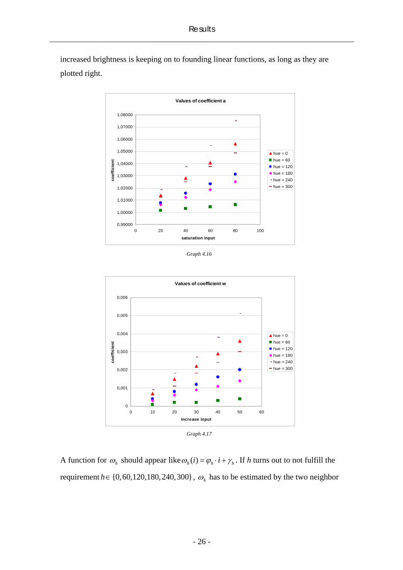
As shown in Graph 4.15, there is a linear trend amongst the data with a precise hue and
saturation, and our first outcast for the brightness function
is , , , ,( , , , ) h s i h s iB h s b i bα β= ⋅ + . The coefficient , ,h s iα can be calculated if the values of
hue and increases brightness are known, since a plot with the coordinate axis
saturation input/ ,h iα also founds a linear trend (Graph 4.16). That function should be
declared as following: , , ,( )h i h i h is sα ω ψ= ⋅ + . The values of coefficient , ,h s iβ do not
show any trend, and they are therefore all exchanged for an average value.
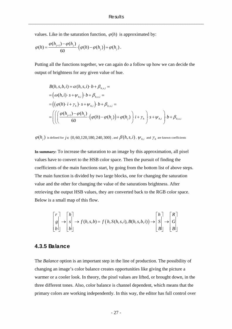
The next step is to create the functions ( , )h iω and ( , )h iψ , so the coefficient ,h iα
(Graph 4.16), and eventually even , ,h s iα , can be calculated with all of the affecting
variables. In Graph 4.17, increased input/ hω is plotted, and the data for the different
values of hue forms a linear trend. Notice that these linear functions do not find the same
order as their corresponding values of hue. It is however clear that the measured data for
Brightnesshue = 0
60
65
70
75
80
85
90
95
100
60 65 70 75 80 85 90 95
input
outp
ut
sat = 0sat = 20sat = 40sat = 60sat = 80
Graph 4.15
Results ___________________________________________________________________________
- 26 -
increased brightness is keeping on to founding linear functions, as long as they are
plotted right.
A function for hω should appear like ( )h h hi iω ϕ γ= ⋅ + . If h turns out to not fulfill the
requirement {0,60,120,180,240,300}h∈ , hω has to be estimated by the two neighbor
Values of coefficient a
0,99000
1,00000
1,01000
1,02000
1,03000
1,04000
1,05000
1,06000
1,07000
1,08000
0 20 40 60 80 100
saturation input
coef
ficie
nt
hue = 0hue = 60hue = 120hue = 180hue = 240hue = 300
Graph 4.16
Values of coefficient w
0
0,001
0,002
0,003
0,004
0,005
0,006
0 10 20 30 40 50 60
increase input
coef
ficie
nt
hue = 0hue = 60hue = 120hue = 180hue = 240hue = 300
s
Graph 4.17
Results ___________________________________________________________________________
- 27 -
values. Like in the saturation function, ( )hϕ is approximated by:
( )1( ) ( )( ) ( ) ( ) ( )
60j j
j j
h hh h h h
ϕ ϕϕ ϕ ϕ ϕ+ −
= ⋅ − + .
Putting all the functions together, we can again do a follow up how we can decide the
output of brightness for any given value of hue.
( )( )( )
( )
, ,
, , ,
, , ,
1, , ,
( , , , ) ( , , )
( , )
( )
( ) ( )( ) ( ) ( )
60
h s i
h i h s i
h h i h s i
j jj j h h i h s i
B h s b i h s i b
h i s b
h i s b
h hh h h i s b
α β
ω ψ β
ϕ γ ψ β
ϕ ϕϕ ϕ ϕ γ ψ β+
= ⋅ + =
= ⋅ + ⋅ + =
= ⋅ + ⋅ + ⋅ + =
⎛ ⎞⎛ − ⎞⎛ ⎞= ⋅ − + ⋅ + ⋅ + ⋅ +⎜ ⎟⎜ ⎟⎜ ⎟⎜ ⎟⎝ ⎠⎝ ⎠⎝ ⎠
( )jhϕ is defined for {0,60,120,180, 240,300}j∈ , and ( , , )h s iβ , ,h iψ and hγ are known coefficients
In summary: To increase the saturation to an image by this approximation, all pixel
values have to convert to the HSB color space. Then the pursuit of finding the
coefficients of the main functions start, by going from the bottom list of above steps.
The main function is divided by two large blocks, one for changing the saturation
value and the other for changing the value of the saturations brightness. After
retrieving the output HSB values, they are converted back to the RGB color space.
Below is a small map of this flow.
( )( , , ) , ( , , ), ( , , , )r h h Rg s f h s b f h S h s i B h s b i S Gb b B B
⎡ ⎤ ⎡ ⎤ ⎡ ⎤ ⎡ ⎤⎢ ⎥ ⎢ ⎥ ⎢ ⎥ ⎢ ⎥→ → = → →⎢ ⎥ ⎢ ⎥ ⎢ ⎥ ⎢ ⎥⎢ ⎥ ⎢ ⎥ ⎢ ⎥ ⎢ ⎥⎣ ⎦ ⎣ ⎦ ⎣ ⎦ ⎣ ⎦
4.3.5 Balance
The Balance option is an important step in the line of production. The possibility of
changing an image’s color balance creates opportunities like giving the picture a
warmer or a cooler look. In theory, the pixel values are lifted, or brought down, in the
three different tones. Also, color balance is channel dependent, which means that the
primary colors are working independently. In this way, the editor has full control over

Results ___________________________________________________________________________
- 28 -
the image’s appearance. He can, for instance, edit the blue channel alone in the tones
of shadows, without affecting any other channel or tone.
When affecting the highlights (Graph 4.18), the plotted data forms a linear trend,
( )f x xα β= ⋅ + . The values for coefficient α can also be expressed in a function
( )i iα ω ψ= ⋅ + , and in Graph 4.19 a polynomial of degree three forms an accurate
approximation. The values for coefficient β do however not show any trend, but they
are rather close. Therefore they can all be exchanged for an arithmetic average. Graph
4.18 and Graph 4.19 are both appliable for the three channels whenever they are active.
When changing the color balance for one channel, the other two turn to inactive
channels, but still are affected. It is however not a big difference, and they form the
same trend line, ( )f x xα β= ⋅ + , no matter level of increase.
Graph 4.18
Highlights, Blue Channel
0
100
200
300
400
500
600
700
-100 100 300 500 700 900 1100
input
outp
ut
50%40%30%20%10%-10%-20%-30%-40%-50%

Results ___________________________________________________________________________
- 29 -
As shown in Graph 4.18, the highest output value of the data ‘10%’ is around 550. It
can seam to be that the measured data have been mixed up, since the highest value of
range should be 1023, but the answer lies in a certain setting in the Nucoda system.
This setting doesn’t really influence anything, since the approximated functions are
provided and can easily be adjusted to compensate for the default setting of the
system.
The midtones operations are the hardest to approximate. The theory here is that only
the pixel values in the middle of the range of {0:1023} will be affected.
As in the Graph 4.20 it is trivial that the function for midtones can be expressed in a
polynomial, and after testing it is shown that a polynomial of degree three could be
satisfying, as in: 3 2( )f x x x xα β ς δ= ⋅ + ⋅ + ⋅ + . All coefficients of this expression
can also be declared in ( )iα , ( )iβ , ( )iς and ( )iδ . But after evaluating this way of
calculating midtones values, it was not satisfying accurate. Therefore this way of
approximation is not being used, and it has been exchanged for an accurate high
degree polynomial approximation for every level of 10%. For every value
where {... 20, 10,0,10,20...}i∉ − − , ( )f x is estimated by the two predefined
neighbour values.
Values of coefficient a
0,35
0,4
0,45
0,5
0,55
0,6
0,65
0,7
-60 -40 -20 0 20 40 60
Increase input
coef
ficie
nt
Graph 4.19

Results ___________________________________________________________________________
- 30 -
The shadows operations are similar to the highlights, they have a linear trend. In fact,
everything about the shadows functions is very much the same as the highlights
functions. The difference is however that the value of increase changes the lower
parts of the linear curve (Graph 4.21), instead for changing the upper parts.
Midtones, Blue Channel
0
200
400
600
800
1000
1200
0 200 400 600 800 1000 1200
input
outp
ut
50%40%30%20%10%No Change-10%-20%-30%-40%-50%
Graph 4.20
Shadows, Blue Channel
0
200
400
600
800
1000
1200
0 200 400 600 800 1000 1200
input
outp
ut
50%40%30%20%10%No Change-10%-20%-30%-40%-50%
Graph 4.21
Evaluation ___________________________________________________________________________
- 31 -
5 Evaluation
In this chapter an evaluation of how well the software is working will be presented.
New patches have been made by the software, and the patches will be compared to
the original ones provided by Nucoda. With graphs and comments on remade patches
a full functionality check will be done. In the evaluation, the software will from now
on be referred as JESSIE - LUT editor or simply as Jessie.
Even if patches with up to 100% of increase have been analyzed, only patches up to
50% will be compared. According to Kamil Rutkowski, any desired change of a LUT
is likely to be around 5-10%. Bigger changes won’t be necessary.
5.1 Brightness and Contrast
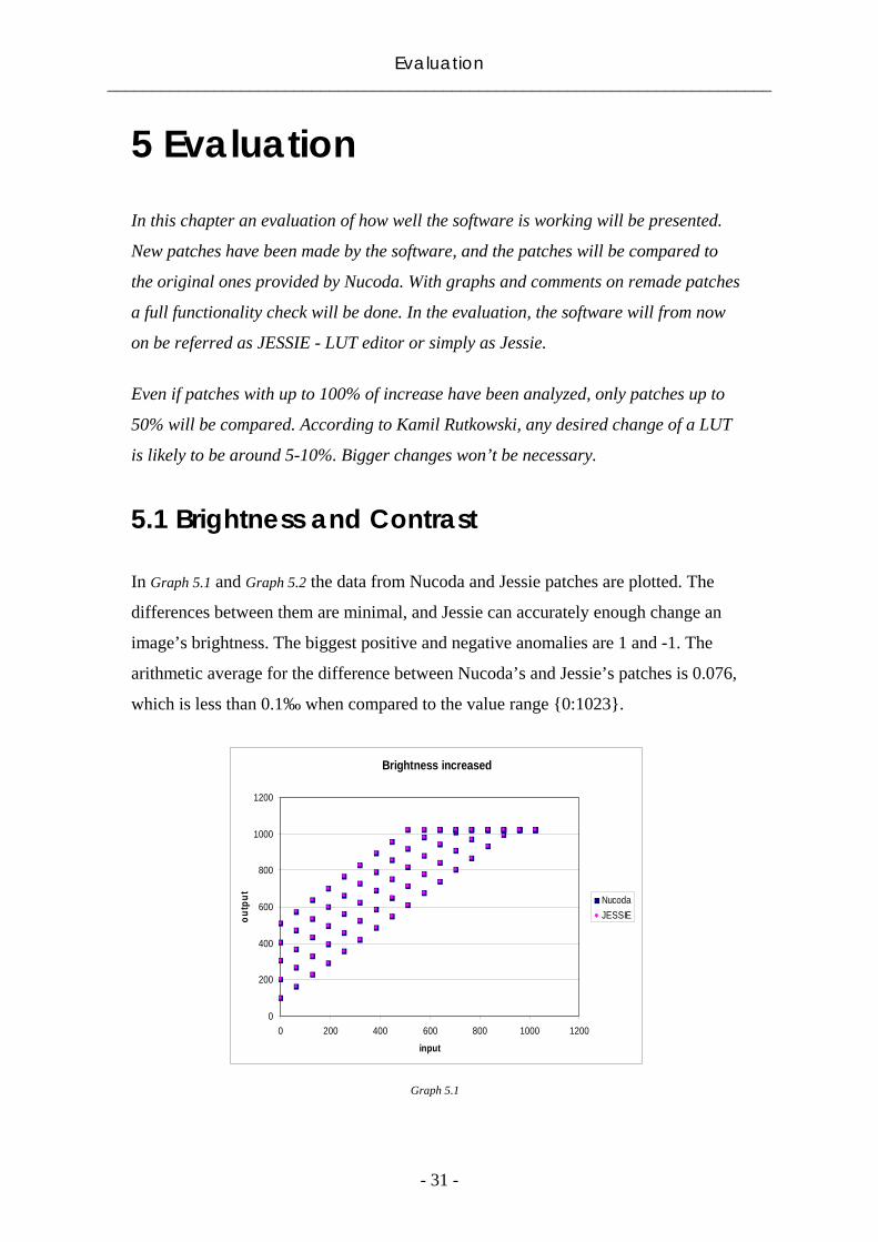
In Graph 5.1 and Graph 5.2 the data from Nucoda and Jessie patches are plotted. The
differences between them are minimal, and Jessie can accurately enough change an
image’s brightness. The biggest positive and negative anomalies are 1 and -1. The
arithmetic average for the difference between Nucoda’s and Jessie’s patches is 0.076,
which is less than 0.1‰ when compared to the value range {0:1023}.
Graph 5.1
Brightness increased
0
200
400
600
800
1000
1200
0 200 400 600 800 1000 1200
input
outp
ut NucodaJESSIE
Evaluation ___________________________________________________________________________
- 32 -
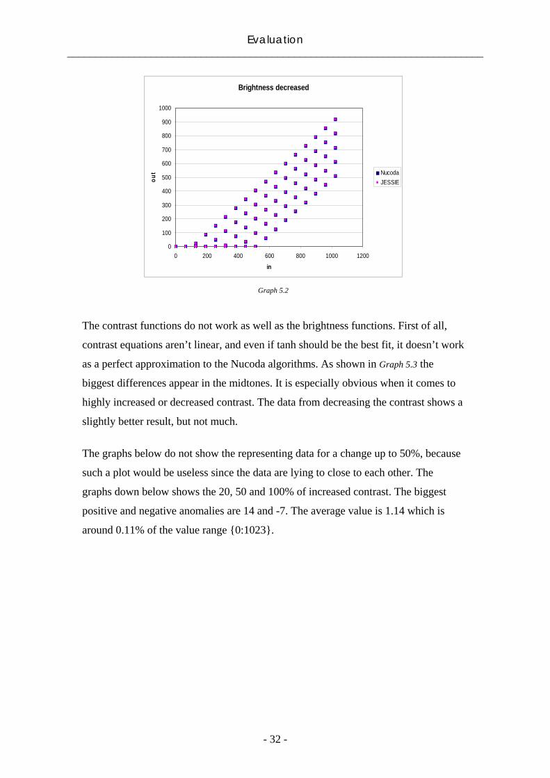
The contrast functions do not work as well as the brightness functions. First of all,
contrast equations aren’t linear, and even if tanh should be the best fit, it doesn’t work
as a perfect approximation to the Nucoda algorithms. As shown in Graph 5.3 the
biggest differences appear in the midtones. It is especially obvious when it comes to
highly increased or decreased contrast. The data from decreasing the contrast shows a
slightly better result, but not much.
The graphs below do not show the representing data for a change up to 50%, because
such a plot would be useless since the data are lying to close to each other. The
graphs down below shows the 20, 50 and 100% of increased contrast. The biggest
positive and negative anomalies are 14 and -7. The average value is 1.14 which is
around 0.11% of the value range {0:1023}.
Graph 5.2
Brightness decreased
0
100
200
300
400
500
600
700
800
900
1000
0 200 400 600 800 1000 1200
in
out Nucoda
JESSIE

Evaluation ___________________________________________________________________________
- 33 -
5.2 Bright regions
The accuracy of the functions for the Bright regions option is varying. Patches have
been created by using the software Jessie, where the amount of increased or decreased
value, in the three different tones, is varied. When compared to the Nucoda patches,
big similarities are discovered. This is plotted in the below graphs.
Graph 5.3
Contrast increased
0
200
400
600
800
1000
1200
0 200 400 600 800 1000 1200
input
outp
ut no changeNucodaJESSIE
Graph 5.4
Contrast decreased
0
200
400
600
800
1000
1200
0 200 400 600 800 1000 1200
input
outp
ut no changeNucodaJESSIE

Evaluation ___________________________________________________________________________
- 34 -
The biggest positive and negative anomalies for the shadows, midtones and
highlights, are {-3, 2}, {-6, 8} and respectively {-1, 3}. The biggest differences can
be found in the midtones patches. By experience, the midtones are always harder to
find a perfect fit for, no matter what kind of option of image editing is used. In the
case of Bright regions, the approximations for highlights, and shadows, take
advantage of the unchanging values in the opposite tone (Graph 4.7, Graph 4.9). The
approximations for the midtones don’t have such an advantage, which will increase
the level of difference between calculated and measured data.
The arithmetical averages for the differences between the Nucoda and Jessie patches,
are for the shadows, midtones and highlights, -0.11, 0.17 and respectively 0.07. These
values correspond to a percental flaw of 0.011, 0.017 and 0.007.
Graph 5.5
Shadows
0
200
400
600
800
1000
1200
0 200 400 600 800 1000 1200
input
outp
ut NucodaNo changeJessie

Evaluation ___________________________________________________________________________
- 35 -
5.3 Saturation
When comparing Jessie patches to Nucoda patches, considerable differences are
discovered. Even if the approximation functions have been created in several steps,
the saturation option in Jessie is still not working well enough for industrial use.
Graph 5.6
Midtones
0
200
400
600
800
1000
1200
0 200 400 600 800 1000 1200
input
outp
ut NucodaNo changeJessie
Graph 5.7
Highlights
0
200
400
600
800
1000
1200
0 200 400 600 800 1000 1200
input
outp
ut NucodaNo changeJessie

Evaluation ___________________________________________________________________________
- 36 -
After converting RGB data to HSB data the values are run through the saturation
algorithms. Whenever the value of s reaches top value, 1023, the value of b is
continues to grow. The values of s and b are dependent on each other, and grows up
to a certain value if the other one stops. This works both ways, so if the value of b
reaches the top value, the value of s will keep going further. These circumstances
were not regarded when creating the approximated functions and it is to this project
unexplored.
After additional comparison, it is obvious that the saturation option is working better
when the saturation is decreased (Chapter 9.3). One explanation is that whenever the
saturation is decreased, both of the values s and b are also decreased. In other words,
none of the values will reach the highest possible value and therefore none of the
variables have to compensate for the other one.
There are also possible complications in converting pixels between color spaces. The
RGB color space, when working with 10 bits, has 1023×1023×1023 possible values.
The HSB color space has 360×100×100 possible values. That makes the RGB color
space about 300 times bigger, which means that many of the HSB values have to be
reused for several values of RGB. This problem was however solved in this project,
since a special object was created while programming. This object makes it possible
to define the HSB color space with enough decimals so every RGB value gets a
unique HSB value when converted. However, when converting the HSB values back
into RGB, the LUT appearance demands integers and there will be possible loss of
accuracy. This is also an explanation why the Jessie patches mismatches with the
Nucoda patches by this magnitude.
5.4 Balance
The Balance option is a powerful tool to dramatically change an image’s appearance.
The differences between the Nucoda and Jessie patches varies, since the Balance
option offers nine possibilities to modify the pixel values, three color channels in
three tones.

Evaluation ___________________________________________________________________________
- 37 -
No graphs are illustrated in this chapter, since a table gives a good idea of how well
the functions are working. Besides, with all the plotted data it would be impossible to
distinguish one from the other. The following table (Table 5.1) gives a good idea of
how well Jessie’s balance option is working. It shows the biggest positive and
negative values for the anomalies between the Nucoda and Jessie. It also shows the
arithmetic average for all the flaws.
Without any surprise, the weak parts in this option are in the midtones. The midtones
are, again, hard to approximate with very high accuracy. However, the midtones are
more accurate than this table is showing, since the table has taken all the data for the
increased input from 50% to -50% into calculation. Up to 20%, all the color channels
are working with the biggest positive and negative anomalies valued to 2 and -3. It is
not likely that anyone in the industry wishes to edit a preexisting LUT to increase or
decrease the color balance more than 5-10%.
Anomalies SHADOWS MIDTONES HIGHLIGHTS
Red Green Blue Red Green Blue Red Green Blue
Biggest Positive 1 2 2 19 21 35 2 2 3
Biggest Negative -2 -1 -2 -11 -5 -5 -4 -3 -4
Avarage -
0.078 0.061 0.025 0.0176 0.327 0.412 0.061 -0.008
-
0.086
Table 5.1
Conclusions ___________________________________________________________________________
- 38 -
6 Conclusions
The main question is if Jessie is working well enough for industry standards. The
answer is “yes”, but however, also “no”. It is obvious that Jessie’s weakness relays in
the saturation option, where the anomalies are most considerable. Why the differences
between the Nucoda and Jessie patches are so big is discussed in Chapter 5.3, and this
evaluation has nothing more to report. The saturation option should though be tested
together with the Nucoda system before getting wiped out from the Jessie software.
Increasing the saturation is a highly complicated operation and maybe pixel values
don’t tell everything. Maybe some of the anomalies compensates for others when the
amount of pixel values increases, and a high resolution image takes place. Even if it
doesn’t look good in numbers, a final check for confirmation should determine
whether or not the saturation option fulfils industry standards.
Another question is if the approximated functions for the contrast option accurate
enough. The anomalies for increased contrast by 10% and 20% are 4 and 6. In my
opinion, a difference of value 4 should be satisfying. The difference of value 6 should
too be satisfying, since contrast is all about differences in color tones. The main
importance is the shape of the trend line. The functions which are in use look really
good in graphs, even if they don’t have a perfect accuracy to the measured data. It
should be further explored by tests with the Nucoda before judged.
The rest of the equations however, and they are more than perhaps can be recognised
by reading the Evaluation chapter, will work perfectly in the industry. The
Brightness, Bright Regions and the, perhaps most importantly, Color Balance options
are working with high accuracy. The one exception is the Balance option when the
midtones are changed. And it’s only not working satisfying when the channels are
increased by over 20%, which is unlikely they will be when Jessie is running
commercially. So the conclusion is that Jessie, LUT editor, is working within industry
standards. Hope lies for the contrast and saturation options to be accurate enough
while testing with the Nucoda system, even if it is likely that the saturation option
never will pass.

Future research ___________________________________________________________________________
- 39 -
7 Future research
A LUT editor with many fully working image editing options is now created, and will
save production time. It is not yet possible however to automatically add two LUTs
together with Jessie, but when it is, long rendering times will be shorten to fractions.
The approximations are done, and only the logical operators in the code are missing.
Since the knowledge exists in how LUT A and B are working, and how they are
affecting the picture, a LUT C can be created by adding the separate functions with
their corresponding values.
It would be interesting to know why the approximations for the Saturation option are
so badly conditioned. One proposal is that the s and b variables need to be further
studied, and probably the effect of the one value’s increase, while the other one
reaches the top value, needs to be taken in consideration. The value for h was set
fixed when increasing the saturation because of lack of trend. But perhaps there is a
trend, yet waiting to be discovered?
The software’s user interface could likely be improved. To do so, perhaps a
questionnaire study could be done, where many people’s input is collected.
Otherwise, some interviews from different image editors could be sufficient, or even
better, since such a questionnaire can be hard to formulate and many participants is
needed.
Another nice feature for a new version of Jessie would be a preview mode of the
actual picture, which updates each time a level is increased in one of the different
options. This sounds rather difficult, since there aren’t that many systems that can
apply a LUT to a project. But perhaps the difficulties can be overcome, and editing
LUTs never have been easier.

References __________________________________________________________________________
- 40 -
8 References
8.1 Books
GONZALEZ, RAFAEL C. WOODS, RICHARD E. 2008. Digital Image
Processing. Pearson Education, Inc. ISBN 0-13-168728-x.
GREEN, PHIL. 1999. Understanding Digital Color, Second edition, GATFPress, ISBN 1-
85802-450-1.
RÅDE, LENNART. WESTERGREN, BERTIL. 1995. BETA – Mathematics
Handbook for Science and Engineering, Third edition, Studentlitteratur, ISBN 91-44-25053-3.
WATKINSON, JOHN. 2001. Convergence in Broadcast and Communications
Media. Focal Press, ISBN 0-240-51509-9.
8.2 Webb
DIGITAL VISION. Digital Vision provides software and hardware equipment for
motion picture editing. http://www.digitalvision.se
POYTON, CHARLES. Frequently Asked Question about Color. http://www.poynton.com/PDFs/ColorFAQ.pdf
WIKIPEDIA. Complete algorithm for conversions between the RGB and HSB color
spaces. http://en.wikipedia.org/wiki/HSV_color_space

Appendices ___________________________________________________________________________
- 41 -
9 Appendices
9.1 Analysis of hexadecimal machinery code
In this example the flow: “802A 5FD7 0000 0800…” will be handled.
[ ] [ ][ ]
16 2
2
802A 5FD7... 1000000000101010 101111111010111...
1000000000 1010101011 1111101011 1...
= =
As one can see, the hexadecimal flow are converted to a binary base and then only
stacked up differently. The second line of binary code has the same ordered as the
first one, but instead of having the flow divided by 16 pieces of digits, it is divided by
10. The first three stacks of binary code on the second line found one pixel value,
with the value of the red (first stack), green (second stack) and blue (third stack) channels.
This is the way of handling the hexadecimal data and retrieving each pixel value.
9.2 Algorithm for conversion between color
spaces
The model for the approximation of the Saturation option requires the data to be
converted from RGB color space to HSB (also known as HSV) color space. That
operation was done by the following algorithm. The variables r, g and b are the
variables for red, green and blue color channels. Their value range are {0:1}. The
variables h, s, and v are the variables for hue, saturation and value (or in this case called
brightness). The value range of h is {0:360}, and for the variables s and v it is {0:100}.

Appendices ___________________________________________________________________________
- 42 -
maxv =
9.3 Saturation anamolies Below are the graphs representing each pixel anomaly for the increased and decreased
saturation by 10%.
Graph 9.1
Saturation increased by 10%
-65
-45
-25
-5
15
35
55
0
Measured pixels
Ano
mal
ies
RedGreenBlue
0,
60 0 mod 360 ,max min
60 120 ,max min
60 240 ,max min
g b
h b r
r g
⎧⎪ −⎛ ⎞⎪ ⋅ +⎜ ⎟⎪ −⎝ ⎠⎪= ⎨ −
⋅ +⎪ −⎪−⎪ ⋅ +⎪ −⎩
max minif =
maxif r=
maxif g=
maxif b=
max 0if =0,max min ,
maxs
⎧⎪= −⎨⎪⎩
max 0if ≠

Appendices ___________________________________________________________________________
- 43 -
Saturation decreased by 10%
-15
-10
-5
0
5
10
0
Measured pixels
Ano
mal
ies
Series1Series2Series3
Graph 9.2
Glossary ___________________________________________________________________________
- 44 -
10 Glossary
Bright Regions The Bright Regions tool for color correction is a powerful way of
affecting the brightness of an image in a certain tone.
Complementary colors The complementary colors are cyan, magenta and yellow. They are
obtained by blending two of the primary colors.
Color Balance Color Balance is a color correction tool, where the appearance of an
image can be affected in the three different color channels red, green
and blue. The tool is also tone dependent and the image can be edited in
the shadows, midtones or highlights.
DPX DPX is an abbreviation for Digital Picture Exchange and is a digital
image file format. It is commonly used in the industry and can save
color information logarithmically in 10bits.
Excel Excel is a program for analysis, calculations and graphical
presentations of data. It is produced by the Microsoft Corporation.
HSB HSB is an abbreviation for the Hue, Saturation and Brightness. It is a
color space formed as a cylinder, where the deep and height is scaled
by the saturation and brightness. The hue is scaled in degrees, formed
as the base circle of the cylinder.
Hue Hue can be considered as a specific color. In the HSB color space it is
scaled from 0 to 360 degrees, where the primary colors are placed at 0,
120 and 240 degrees.
Jessie Jessie (LUT editor) is the produced software for this project. It can
open LUTs, edit them, and export the changes into new LUTs.
Lookup Table A Lookup Table is a text file containing pixel values data. It can be
considered as a layabout for color correction, which is applied to the
picture through a video editing software.
LUT LUT is an abbreviation for Lookup Table.
Glossary ___________________________________________________________________________
- 45 -
MatLab MatLab is an analysis and calculation software provided by
Mathworks.
Nucoda The Nucoda is a video editing software, provided by Digital Vision. It
was the software which was used during this project.
Primary colors The primary colors are red, green and blue.
RGB RGB is an abbreviation for the three primary colors Red, Green and
Blue. RGB is a cubic color space, where every possible color is defined
by mixing the primary colors.
Saturation Saturation has several definitions. In this project it was approached as
how the HSB color space is defined. The saturation scale for a certain
color is here explained as it goes from white to a fully saturated state,
where the color reaches its full vividness.

TRITA-CSC-E 2008:080 ISRN-KTH/CSC/E--08/080--SE
ISSN-1653-5715
www.kth.se