arX

iv:h

ep-t

h/05

0311

2v2

2 J

un 2

005

hep-th/0503112

Long strings in two dimensional string theoryand non-singlets in the matrix model

Juan Maldacena

Institute for Advanced Study, Princeton, NJ 08540, USA

We consider two dimensional string backgrounds. We discuss the physics of long

strings that come from infinity. These are related to non-singlets in the dual matrix model

description.

1. Introduction

The main motivation for this paper is to get some insights about the Lorentzian

physics of the two dimensional black hole [1]. A proposal for the matrix model dual of

the Euclidean black hole was made by Kazakov, Kostov and Kutasov in [2]. These au-

thors proposed a matrix model description which involves adding Wilson lines for the

ordinary gauged matrix model that describes the two dimensional string background [3].

This implies that we need to understand the matrix model in its non-singlet sector. In

this paper we study aspects of the physics of the matrix model in its non-singlet sec-

tor. While we will not give a picture for the two dimensional black hole, the remarks in

this paper might be helpful in this quest. Further work on this correspondence includes

[4][5][6][7][8][9][10][11][12][13][14][15][16][17].

We will show that the double scaling limit of the matrix model in its simplest non-

trivial representation, the adjoint representation, is related to a two dimensional string

background with a folded string that comes in from the weak coupling region and goes back

to the weak coupling region. Such a string is not static. Indeed, we get a time dependent

configuration. In the double scaling limit, the system does not have a well defined ground

state but it has interesting time-dependent solutions. An interesting observable is the

scattering amplitude for a folded string that comes from the weak coupling region and

goes back to the weak coupling region1. This phase can be computed exactly at tree level

in string theory using formulas in [20]. We compare this to the matrix model computation.

We reduce the matrix model computation to a rather simple looking eigenvalue problem.

Though we were not able to solve completely this eigenvalue problem we could show

that in the two asymptotic limits of high and low energies, the answer matches with the

corresponding exact expressions in string theory. Previous work on the non-singlet sector

includes [21,22]. This picture of the non-singlet sector is important for understanding

the physical meaning of the results of computations done via T-duality or the Euclidean

worldsheet theory.

We consider the same problem also in the type 0A/0B superstring cases, where a new

feature arises. There are two answers that depend on the treatment of a particular fermion

zero mode.

This paper is organized as follows. In section 2 we discuss the physics of long strings

in two dimensional string theory. In section 3 we consider non-singlets in the hermitian

1 Folded strings have also been previously studied in [18] [19].

1

matrix model. We first concentrate on the adjoint representation and then we discuss some

features for general representations. In section 4 we consider non-singlets in the complex

matrix model that is dual to 0A superstring theory. We end with a discussion.

2. Long strings in two dimensional string theory

2.1. Classical strings in two dimensions

Let us first consider a simple problem [18]. Suppose we have a classical string on a two

dimensional spacetime parametrized by X0, φ. We choose a gauge with ∂+X0 = ∂−X

0 = 1

with ∂± = ∂τ ±∂σ , where τ, σ are the worldsheet coordinates. The classical equations then

reduce to ∂+∂−φ = 0 and the Virasoro constraints

−1 + (∂+φ)2 = 0 , −1 + (∂−φ)2 = 0 (2.1)

Then we conclude that ∂+φ = ±1. The first derivative does not have to be continuous.

So the most general solution has the form φ = φ+(σ+) + φ−(σ−) where φ+ and φ− are

periodic functions with the same period and with derivative piece-wise equal to ±1. A

simple example would be

φ+(s) ≡ φ−(−s) ≡ |s− L/2| , for 0 < s < L (2.2)

and defined in a periodic fashion outside this interval. This describes a pulsating string.

At X0 = 0 the string is folded and stretched to its maximum length L from φ = 0 to

φ = L. At later times the two folds start moving towards each other at the speed of light,

they cross at X0 = L/2 and they end end up with a configuration similar to the original

one at X0 = L. See figure 1. We can think of the whole configuration as two massless

particles joined by a string. In fact, the energy levels that we get are similar to those we

get for mesons in 2d QCD with massless quarks at high excitations levels [23]2. Here we

looked at a simple solution, but the string can have many folds, see [18][19] for further

discussion.

2 In 2d QCD we have an open string rather than a folded string but the form of the solutions

is essentially identical.

2

Time

φ

Fig. 1: Two dimensional pulsating string. The ends of the string move at the

speed of light.

2.2. Long strings with a linear dilaton

Now let us consider the situation with linear dilaton, Φ = Qφ. Then the Virasoro

constrains in (2.1) are replaced by3

−1 + (∂+φ)2 −Q∂2+φ = 0 , −1 + (∂−φ)2 −Q∂2

−φ = 0 (2.3)

Solving these equations we find

φ = φ0 −Q log coshσ+

Q−Q log cosh

σ−

Q= φ′0 −Q log(cosh

τ

Q+ cosh

σ

Q) (2.4)

This is the most general solution after we allow shifts of τ and σ. The solution correspond-

ing to the usual pointlike string, where φ = ±τ , can be viewed as a limit of this solution.

Except for this special limit, the solution (2.4) is not periodic. It represents a folded string

stretched to minus infinity in the φ direction. The tip of the string moves from the weakly

coupled region into strong coupling and back into the weakly coupled region. One minor

difference with the strings discussed in the previous section is that in this case the tip of

the string looks a bit more like a massive particle, with a mass of order QMs. After a few

string times the tip of the string is accelerated to nearly the speed of light so that its mass

becomes unimportant. Note that we do not have oscillating strings. This agrees with the

fact that, for Q = 2, there are no closed string states in the linear dilaton region other

than the massless “tachyon”.

3 Throughout this paper we set α′ = 1 for the bosonic string and α′ = 12

for the superstring.

3

φφφc m

Fig. 2: Long string coming in from φ = −∞ and bouncing back. The vertical

direction is time and we show snapshots at different times. The strings stretch

from φ = −∞, or a large negative cutoff value φc. The tip comes from the left

and, after it reaches the largest value of φ = φm, it starts moving back to the left.

We can think of this string as a particle (the tip of the string) with a linear potential

(provided by the string tension). This enables us to use a WKB approximation for the

wavefunction. The particle momentum and wavefunction are given by

p = ±21

2π(φm − φ) , ψ ∼ ei

∫

dφp ∼ e±i 12π

(φ−φm)2 (2.5)

where we used the relativistic dispersion relation that is valid for p ≫ 1. In (2.5) we also

used that the force is given by twice the tension since the string is folded. Here φm is just

an integration constant which is the value of φ at which the tip of the string bounces back.

This is then related to the energy of the string through

E = 21

2π(φm − φc) , ǫ ≡ E −Ediv =

1

πφm , Ediv = − 1

2πφc (2.6)

where φc is some cutoff at large negative values. We have defined the finite energy ǫ by

subtracting a divergent piece. This divergence arises because the string is stretching all

the way to φ→ −∞.

In the φ → −∞ region, (2.5) will be a correct approximation for the full wavefunc-

tion. We will check this statement later both on the matrix model side and in the exact

worldsheet analysis. So we can define the scattering amplitude through4

ψ = e−i 12π

(φ−φm)2 − eiδei 12π

(φ−φm)2 (2.7)

4 This is a somewhat non-standard definition of the phase. The relation to the more standard

definition can be found in appendix A. This is a detail most readers will want to ignore in a first

reading.

4

In this definition, φm is just a constant related to the energy ǫ of the string through (2.6).

In the linear dilaton region we see that the phase (2.7) is independent of the energy since

it depends only on the behavior of the wavefunction for φ ∼ φm and φm drops out of this

problem. In other words, the essential physics of this problem is translation invariant and

it does not matter precisely where the string bounces back. We will define the constant

relative phase between the two terms in (2.7) in such a way that this constant is zero

eiδ = 1 (2.8)

2.3. Strings in (Liouville)×(Time)

Let us now consider the Liouville case. The general solution of the classical Liouville

equation can be written as

µe2bφ =1

[∑

i f+i (bσ+)f−

i (bσ−)]2(2.9)

where fi obey the conditions

∂2fi − fi = 0 , ǫijfi∂fj = 1 (2.10)

The first comes from (2.3), with Q = 1/b+ b ∼ 1/b, where we assume that b is small which

is the classical limit. The second equation in (2.10) comes from the Liouville equation. We

then conclude that the most general solution is

µe2bφ =4

(Aebσ++bσ− +Bebσ+−bσ− + Ce−bσ++bσ− +De−bσ+−bσ−)2(2.11)

where AD − BC = 1. Some particular interesting cases are A = D = 1 B = C = 0. In

this case we get

µe2bφ =1

cosh2 bτ(2.12)

where τ = σ+ + σ−. In this case we can compactify the σ direction. This is the standard

solution representing a small string coming in from infinity. The spacetime energy of the

string is related to the size of the σ circle. If we rescale this circle so that it has standard

length 2π, then we also have to shift φ, since scale transformations also act on the Liouville

field. Then we see that the maximum value of φ is related to the energy of the incoming

particle [3]. Another interesting solution is a = d = cosh γ and b = c = sinh γ then the

solution is

µe2bφ =1

(cosh γ cosh bτ + sinh γ cosh bσ)2(2.13)

This represents the string coming from infinity and going back to infinity. For α = 0 we

get (2.12) (with Q ∼ 1/b). In the limit α → ∞ we get back (2.4). In this case the string

“bounces back” before it gets to the region where the Liouville potential is important.

5

2.4. Exact worldsheet results for the scattering of long strings

An interesting observable for these strings is the scattering amplitude for the strings

to go in and come back to infinity. At the classical level (in the gs expansion) this is just

a phase. We can compute this phase exactly in α′ by using the results for the disk two

point functions in [20]. So we introduce an FZZT brane [20,24] that is extended in φ but

with µB ≫ √µ so that it dissolves at a very large negative value of φ ∼ − logµB . Then

we consider an open string living on this D-brane. We send in the open string towards

the strong coupling region with high energy E0. When the open string reaches the region

φ ∼ − log µB, its ends get stuck in this region while the bulk of the open string stretches as

in the solutions we considered above. Eventually the energy of the stretched string becomes

equal to the initial energy. At this point the string will stretch between φc ≡ − logµB to

φm ∼ E0π − log µB (see the related formula (2.6)). If we take a limit with

E0 → ∞, µB → ∞ , ǫ = E0 −1

πlog µB = finite (2.14)

then we get the problem that we are interested in. Namely, we have an infinitely stretched

string that comes in from infinity and goes back to infinity. We are introducing the FZZT

branes and the open strings on them in order to be able to use the formulas in [20] to

compute the amplitude we are interested in. Starting with the open string two point

function in [20] and performing the scaling limit in (2.14), we obtain the scattering phase

(see appendix A for details)

δ(ǫ) = −∫ ǫ

−∞dǫ′(

πǫ′

tanhπǫ′+ πǫ′

)

ǫ ≡ ǫ+1

2πlogµ

(2.15)

The answer is a function of ǫ. This can be understood as follows. The Liouville potential

becomes important at φL ∼ −12 logµ. The energy ǫ is related to the point were the

string would stretch to a maximum in the absence of Liouville potential by (2.6). So the

amplitude is just a function of φm −φL, which is proportional to ǫ. We see that the phase

δ(ǫ) → 0 for ǫ → −∞, so that we recover the linear dilaton result (2.8). In fact, the

asymptotic behavior of this phase is

δ(ǫ) ∼ (ǫ− 1

2π)e2πǫ = (ǫ− 1

2π)µe2πǫ , for ǫ≪ logµ (2.16)

6

We see that the leading corrections to the ǫ → −∞ answer has the form we expect.

To leading order we get that the phase is zero, in agreement with (2.8), and the first

correction can be interpreted as resulting from the insertion of a cosmological constant

operator. Indeed, in this case the string bounces back before it gets to the region where

the Liouville potential is important. On the other hand, the high energy behavior is

δ(ǫ) ∼ −πǫ2 + (ǫ+1

2π)e−2πǫ , for ǫ≫ logµ (2.17)

The leading result in (2.17) can also be easily understood. We can think of the Liouville

potential as a sharp wall at φL = −12 logµ. This imposes a boundary condition on the

wavefunction at this point, say ψ(φL) = 0. From (2.7) we see that this implies that

δ ∼ − 1

π(φL − φm)2 = −πǫ2 (2.18)

which is just the leading behaviour of (2.17). Note that if the energy gets extremely large,

ǫ ∼ µ, then we expect that this approximation would fail, since that is enough energy to

create a ZZ brane. But for large µ there is a large range of energies, µ≫ ǫ≫ logµ, where

we can trust (2.17).

2.5. Worldsheet formulas for the two dimensional type 0 superstring

For the type 0 superstring formulas we set α′ = 12 . By starting with the exact

Liouville formulas in [25] and taking a limit where µB → ∞ we find two possible results

(see appendix A)

δ+(ǫ) = −2

∫ ǫ2

−∞dǫ′πǫ′(tanh ǫ′π+1) , δ−(ǫ) = −2

∫ ǫ2

−∞dǫ′πǫ′(

1

tanh ǫ′π+1) (2.19)

with

ǫ ≡ ǫ+1

πlogµ (2.20)

The first thing we need to understand is why we get two different results. Let us first look

at the behavior of (2.19) for ǫ≪ 0. To leading order both results give us that δ = 0, which

agrees with the result one expects in the linear dilaton region. The first correction is

δ± ∼ ∓(ǫ− 1

π)eπǫ = ∓(ǫ− 1

π)µeπǫ , ǫ≪ 0 (2.21)

7

So the only difference in the two results is the overall sign. In the linear dilaton region the

field φ is given by (2.4). In a gauge where the worldsheet fermion ψ0 = 0 we also need to

set to zero the supercharge in the φ direction. This will lead to the equation

ψφ+∂+φ−Q∂+ψ

φ+ = 0 (2.22)

and a similar equation for left movers. The only solution to (2.22) is

ψφ+ =

1

cosh σ+

Q

ǫ0 (2.23)

where ǫ0 is a constant. It can be checked that this mode is in the cohomology, namely

it is not given by acting with the supercharge on the original configuration (2.4). Upon

quantization, the left and right moving modes ǫl,r0 together lead to a two dimensional

Hilbert space (ǫl,r0 ∼ σ1,2, where σi are Pauli matrices). The cosmological constant term

µψφ+ψ

φ−e

2φ reduces to σ3µe2φ when it is projected onto the two dimensional space Hilbert

space. So we see that we will get two different answers. When the scattering occurs in the

large negative φ region the leading correction comes from inserting just one cosmological

constant operator and this leads to the two possible signs in (2.21).

The results in (2.19) were actually obtained by scattering NS open strings on an FZZT

brane with η = ±1. Recall that η is a sign which relates the left moving to the right moving

supercharge at the boundary of the worldsheet. We are using the conventions of [25] where

the ZZ brane has η = −1. The sign of η is telling us the relative sign between the left

and right moving fermion. Since the cosmological constant term goes as µψLψRe2φ, the

relative sign between the left and right moving fermion determines the sign of the first

correction. The precise boundary conditions at the end of the string should impose that

only one of the two states associated to the fermion zero modes we discussed above are

kept. We have not worked out the details of how this happens, but it follows from the

results in [25].

The results are basically the same in type 0A and 0B theories, though some of the

detailed properties of the FZZT branes are different.

We can also consider the scattering of Ramond open strings ending on FZZT branes

with different η. In the µB → ∞ limit that we are considering we find results as in (2.19).

8

3. Non-singlets in the matrix model

In this section we consider the SU(N) gauged quantum mechanics of a single hermitian

matrix Φ with the insertion of a Wilson line in the representation R

Z =

∫

DΦDAe∫

dtTr[(D0Φ)2−V (Φ)]TrRei∫

A (3.1)

When we analyze this model we can equivalently set A0 = 0 and consider only states in

the Hilbert space of the matrix Φ that transform in the representation R†. From now

on we will replace R → R† for notational convenience. This problem was considered in

[26,21,22,27,28,29] 5. Of course, the representation R should be such that it can be con-

structed by taking multiple products of the adjoint representation. So the representation

should be invariant under the center of SU(N). We are going to be interested in taking the

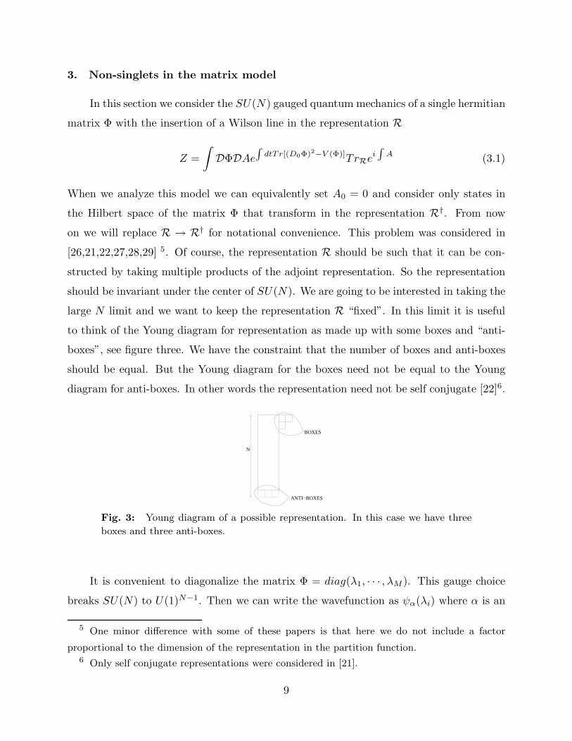
large N limit and we want to keep the representation R “fixed”. In this limit it is useful

to think of the Young diagram for representation as made up with some boxes and “anti-

boxes”, see figure three. We have the constraint that the number of boxes and anti-boxes

should be equal. But the Young diagram for the boxes need not be equal to the Young

diagram for anti-boxes. In other words the representation need not be self conjugate [22]6.

BOXES

ANTI−BOXES

N

Fig. 3: Young diagram of a possible representation. In this case we have three

boxes and three anti-boxes.

It is convenient to diagonalize the matrix Φ = diag(λ1, · · · , λM). This gauge choice

breaks SU(N) to U(1)N−1. Then we can write the wavefunction as ψα(λi) where α is an

5 One minor difference with some of these papers is that here we do not include a factor

proportional to the dimension of the representation in the partition function.6 Only self conjugate representations were considered in [21].

9

index in the representation R, which labels the states with zero weight in this represen-

tation, namely states with zero U(1)N−1 charges. The restriction to zero weight states

comes from integrating out the diagonal part of the gauge field A0. The hamiltonian is

H =

n∑

i=1

−1

2

∂2

∂λ2i

− 1

2λ2

i +1

2

∑

i6=j

TRij T

Rji

(λi − λj)2

P0 (3.2)

where P0 is the projector on to states in the representation R with zero U(1)N−1 charges.

From now on we will drop it. TRij are the matrices corresponding to the ij generator of

SU(N) in the representation R.

3.1. The adjoint representation

This case was considered for a general potential in [26]. Here we review their procedure

and we will further explore it in the case of the inverted harmonic oscillator, where some

of its features were discussed in [21]. The adjoint representation is just given by a matrix

W ji . The states with zero weight are diagonal matrices W j

i = wiδji , with

∑

i wi = 0. We

see that the projection to zero weight states reduced the number of states from N2 − 1 to

N − 1.

We will now treat the interaction in (3.2) perturbatively. To zeroth order we neglect

it and the Hamiltonian is just that of free fermions, with the usual ground state. This

ground state is degenerate since we can choose any state W in the representation. To

first order the interaction term in (3.2) removes this degeneracy. We can think of the

representation part of the wavefunction as given by a state vector |W 〉 =∑

i wi|i〉 × |i〉Then the interaction part of the Hamiltonian acts as

Hint|W 〉 =

N∑

i=1

N∑

j=1, j 6=i

(wi − wj)

(λi − λj)2

|i〉 × |i〉 (3.3)

The interaction Hamiltonian is positive definite. This is most easily seen by computing

〈W |Hint|W 〉. After introducing the eigenvalue density in the standard way and writing

wi → w(λ) we end up with the following eigenvalue problem

Ew(λ) =

∫

dλ′ρ(λ′)w(λ) − w(λ′)

(λ− λ′)2(3.4)

It looks like the lowest energy state is w(λ) =constant. However, this state is not in the

adjoint representation which is constrained to have∫

dλρ(λ)w(λ) = 0. Some approximate

solutions to this problem can be found in [26].

10

Here we are interested in understanding the inverted Harmonic oscillator potential.

In this case it is more convenient to introduce a slightly different variable

h(λ) = w(λ)ρ(λ) (3.5)

In terms of this variable the eigenvalue problem we need to solve becomes

Eh(λ) = − ρ(λ)

∫

dλ′1

(λ− λ′)2h(λ′) + v(λ)h(λ)

v(λ) ≡∫

dλ′ρ(λ′)

(λ− λ′)2

1 =

∫

dλ

ρ(λ)h2(λ)

(3.6)

where we have also included the form of the normalization condition7. In all integrals we

should take the principal value, which means that we subtract all divergent terms when

λ′ → λ. The first term (3.6) can be viewed as a kinetic term and the second as a potential.

This potential contains a constant divergent term plus a finite term. Let us first understand

the problem in the asymptotic region where λ≫ √µ, we will later discuss the more general

case. In the asymptotic region we can approximate ρ(λ) = 1πλ and define τ ≡ logλ. We

obtain

v(λ) =1

π

∫ λc

0

dλ′λ′

(λ′ − λ)2∼ 1

π(τc − τ − 1) (3.7)

where τc is some large cutoff value of τ . The divergence comes from the eigenvalues that

are far away, at large λ′. The region λ′ ∼ λ does not lead to a divergence because we are

using a principal value prescription. So, up to the divergent term we find a linear potential

that is pushing the particle to the large τ region. Similarly we can study the kinetic term

in the asymptotic region and we find that the normalization condition and the kinetic

term, K, become

∫

dτh2(τ) = 1 , (Kh)(τ) = − 1

π

∫

dτ ′h(τ ′)

(2 sinh( τ−τ ′

2))2

(3.8)

Since the kinetic term became translational invariant it is reasonable to solve the problem

using plane waves. Computing the kinetic term in Fourier space we find

K(k) = − 1

π

∫ ∞

−∞dτ

cos kτ

4 sinh2 τ2

=k

tanh(πk)(3.9)

7 Note that v(λ) in (3.6) is not the same as V (λ) in the original matrix model Lagrangian.

11

where we take the principal part of the integral (i.e. we disregard terms that diverge as

τ → 0). At large k we have a relativistic relation

E ∼ |k| for |k| ≫ 1 (3.10)

So we see that the Hilbert space spanned by the vector wi can be thought of as the

Hilbert space of the particle that lives at the tip of the string. The string provides the

linear potential (3.7). It is interesting to see how the dynamics of this extra particle is

generated out of the interaction with the background fermions. The coefficients in (3.7)

and (3.9) match precisely with our expectations based on the string theory discussion after

we identify τ ∼ −φ, where φ is the Liouville direction. This is a standard identification

valid for large values of τ [3]. In fact, the divergence in (3.7) is related to the fact that

the string is stretched all the way to φ = −∞. We can solve the complete quantum

scattering problem in this asymptotic region and one finds a result that agrees with (2.8),

see appendix B.

A few remarks are in order. First, note that, after subtracting the infinite additive

constant (3.7), the spectrum is unbounded below 8. This has some important consequences

when we examine the physics of this model. Second, the infinite constant that we are

subtracting behaves as

Ediv ∼ 1

πτc = − 1

πφc (3.11)

There is precise agreement in the coefficient of this divergent term between the matrix

model and string theory.

Now let us come back to the general problem in (3.6) and include the µ dependence.

It is convenient to define the τ variable through λ =√

2µ cosh τ . Then ρ(λ) =√

2µ sinh τ .

We define h(−τ) ≡ −h(τ) for τ > 0. The sign in this definition is motivated by the fact

that we expect a boundary condition h(τ = 0) = 0, since at τ = 0 we run out of fermions

which could carry the adjoint indices. With this definition of h for negative values of τ we

can extend the range of the integral over the whole τ axis and obtain a simple expression

8 The authors of [21] stated that the spectrum has a gap of order log Λ/µ (which is the

infinite subtraction we are performing) and then a continuum spectrum similar to that of the free

fermions. What is important is that this continuous spectrum is unbounded below.

12

for the kinetic term. Namely, the same as the one we had in (3.8). We also subtract the

divergent piece of the energy. The eigenvalue problem then becomes

ǫh(τ) = − 1

π

∫ ∞

−∞dτ ′

h(τ ′)

4 sinh2 τ−τ ′

2

+ v(τ)h(τ)

v(τ) = − 1

π

τ

tanh τ

(3.12)

with

ǫ = E − 1

πτc +

1

π= E +

1

πlog λc +

1

2πlogµ+ const = ǫ+

1

2πlogµ (3.13)

where ǫ should be thought of as the renormalized energy since it is the one defined with a µ

independent subtraction procedure. We have absorbed some constants in this subtraction

in order to make formulas look simpler. Note that µ has completely disappeared from

(3.12), which agrees with the µ dependence of the string theory result (2.15). The energy

ǫ defined in (3.13) agrees with the renormalized energy defined in (2.6) or (2.14), up to

an additive numerical constant which we have fixed by comparing the matrix model and

the string theory answers. In summary, the energy ǫ which appears in (3.13) should be

directly identified with ǫ in (2.15).

We have been unable to solve the problem of computing the phase directly from (3.12).

Nevertheless we conjecture that the scattering phase that comes out of it is given by

δ(ǫ) = −∫ ǫ

−∞

(

πǫ′

tanhπǫ′+ πǫ′

)

(3.14)

with a definition of the scattering phase analogous to (2.7). We have computed explicitly

the two asymptotic limits, ǫ→ ±∞, as well as the first exponential subleading correction in

each of these asymptotic regions and checked that they match (2.16)(2.17). See appendix

B for details. It seems very likely that there is a simple way to solve this problem exactly

to derive (3.14).

3.2. The vortex anti-vortex correlator

So far we have been discussing the Lorentzian theory. Let us now consider the Eu-

clidean theory with euclidean time compactified on a circle of radius R. Thus we compute

the thermal partition function for the matrix model in the adjoint representation. On the

worldsheet it is easy to compute it. It is given by the two point function for two winding

13

strings. Let us first perform an approximate qualitative analysis. The Liouville correlation

function involves an integral of the from

∫

dφe−µe2φ

e2(2−R)φe−4φ (3.15)

The last term comes from the dilaton. We see that this diverges at weak coupling as∫

dφe−2Rφ. This divergence, which has a positive coefficient, is related to the energy of

the stretched string. In other words, expect a divergence of the form∫

dǫe−(2πR)ǫ for

ǫ → −∞. This divergence is related to the fact that, after the subtraction, the spectrum

of the matrix model Hamiltonian is unbounded below. This divergence is independent of

µ. If we concentrate only on µ dependent terms, then we can get a finite answer. We

can compute this by taking a derivative with respect to µ of (3.15). This then gives a

convergent integral for R < 1

∂µ〈2pt〉 ∼ −∫

dφe−µe2φ

e2φ(1−R) ∼ −µR−1Γ(1 −R) (3.16)

This has just been an approximation to the true answer. The correct answer is computed

using the exact expression for the Liouville three point function in [30]. After taking the

limit b→ 1 in the formulas in [30] we obtain

∂µ〈2pt〉Liouville = −〈3pt〉Liouville = −µ1−R

πR2 Γ(−R)2

Γ(R)2(3.17)

This implies that the two point function in the full string theory is then given by

〈2pt〉 = −2R2µR Γ(−R)2

Γ(R)2∼ Zadj

Zsinglet(3.18)

up to a (positive) numerical constant. Going from (3.17) to (3.18) we loose one factor of R

from integrating (3.17) and we gain one factor of (2πR) from the X path integral. Notice

that this formula is consistent with the statement that the free energy in the adjoint differs

from the singlet free energy by a logarithmic term

Fadj ∼ Fsing −1

2πlogµ (3.19)

Note that the coefficient of the logarithmic term agrees precisely with the matrix model9,

due to the agreement in the divergent parts of the energy that we checked above, see

9 The computations in [21,22] were off by a factor of two.

14

(3.11). The sign in (3.18) seems puzzling. Naively one would have expected the partition

function in the adjoint representation to be positive. What happens is that we have made

an infinite subtraction due to the fact that the spectrum is unbounded below.

Now we would like to compare (3.18) with the matrix model answer. We are interested

in computing the matrix model partition function in the adjoint representation. The matrix

model answer depends on the scattering phase (3.14). We are then lead to a partition

function for the adjoint of the form Zadj ∼ ZsingZW , where Zsing is the singlet partition

function and ZW is the partition function for the effective particle we are considering now.

ZW =

∫

dǫ∂ǫδ(ǫ)

2πe−2πRǫ = −µR

∫ ∞

−∞dǫ

1

2ǫ(

1

tanhπǫ+ 1)e−2πRǫ = − 1

4 sin2 πRµR =

= − µR

4π2Γ(−R)2R2Γ(R)2

(3.20)

We see that we reproduce (3.18) up to factors that are analytic in R for positive R. The

difference between (3.17) and (3.20) is reminiscent of the leg factors that appear when

one compares scattering computations in string theory and the matrix model [3] but it

is different in detail10. (3.20) is the correct normalization for the partition function of

the adjoint since we constructed it explicitly as a trace over the Hilbert space. This

normalization still has an ambiguity due to the precise constant in the subtraction of

the energy. This means that that we can replace µ → µc where c is an R independent

numerical constant. Notice that the poles at integer values of R in (3.20) arise because

when R is an integer we have a new divergence in the computation of the free energy

since the integrand in (3.20) does not decay fast enough at infinity. This implies that a

new subtraction becomes necessary. The coefficients of these divergent terms are integer

powers of µ.

We now consider the problem from a slightly different point of view. Let us consider

an FZZT brane extended in time and compute its cylinder diagram. This diagram contains

a contribution from the exchange of closed strings that are wound in the time direction.

We can pick out the contribution from strings that wind precisely once as follows. The

cylinder diagram is (up to a positive normalization constant)

Zcyl ∼ 2πR∑

n

∫ ∞

0

dEcos2(σπE)

sinh2 πE

1

E2 + n2R2(3.21)

10 The leg factor that we need in this case to match the matrix model answer (3.20) to the

string theory answer (3.18) is Γ(R)−2 for each vertex operator, which looks different than the

momentum leg factors, which are Γ(−|p|)Γ(|p|)

(and we would set p = R).

15

The integer n is summing over the closed string exchanges with strings that are wound n

times, so we will be interested in the term with n = 1. We disregard the pole at E = 0

and all other terms that are µ independent. We can rewrite the integral in (3.21) as an

integral from −∞ to ∞. Then we split the cosine into e2iσE and its complex conjugate.

Both terms give the same answer. For large σ it is convenient to shift the contour of the

first to E → i∞. In this process we pick up poles at E = im and E = inR. If 0 < R < 1

the leading pole appears at E = iR and its residue gives

Z = −2π2e−2σπR 1

sin2 πR∼ −µR(µB)−2R 1

sin2 πR(3.22)

Note that also from this point of view we get a negative sign, in agreement with the

worldsheet computation. Note that here, also, we started with (3.21) which is manifestly

positive and, due to a subtraction, we ended up with a negative answer. The precise

agreement between (3.22) and (3.20) is simply a consistency check, since it is related to

the fact that we assumed that the scattering phase in the matrix model agrees with the

scattering phase in string theory.

We could take a scaling limit where we put Nf FZZT branes and then take

NF , µB → ∞, λ ≡ Nfµ−RB = fixed (3.23)

(3.22) gives a finite source for the winding modes. This procedure would give a source

only for the first winding mode. We should then identify λ with the term in the euclidean

action considered in [2]

S = S0 + λT r(

e∫

A)

+ λT r(

e∫

A)†

(3.24)

Thinking of (3.24) as a limit of (3.23) has the advantage that we start from system with a

clear Lorentzian interpretation, at least on the string theory side, which in the limit (3.23)

leads us to consider the partition function for the action (3.24) studied in [2]. So the two

dimensional string theory in the presence of Nf FZZT branes might be a good starting

point for thinking about the Lorentzian version of the two dimensional black hole [1].

16

3.3. All orders result via T-duality

We expect the all orders partition function for the adjoint representation will be given

the correlator of two strings with winding numbers one and minus one. We can compute

this in the following indirect way. From the string theory point of view we can assume

that T-duality is a good symmetry. On the T-dual side, this translates into a computation

for momentum correlators. We can compute these using the matrix model fermions of

the T-dual model, which are free since we are simply computing correlators of momentum

operators. This is just a computation in the singlet sector and can be done using the

general formulas in [31]. The matrix model fermions of the T-dual model should not be

confused with the original matrix model fermions. T-duality is not an obvious symmetry

of the matrix model. We find, see details in appendix D,

Z ∼ Zsing

(

Γ( 12

+ iµR + R2)Γ( 1

2− iµR + R

2)

Γ( 12− iµR − R

2)Γ( 1

2+ iµR − R

2)

)1/2

(3.25)

up to non perturbative terms in 1µ, which is us much precision as we can hope for the

bosonic string case. The correlator (3.25) is simply the momentum correlator in the T

dual matrix model written in terms of the original variables. The result (3.25) differs from

the result in [22] by the overall power (instead of 12

in the exponent they had 14

11). On the

T-dual matrix model we know that there are leg factors that need to be taken into account.

Notice also that (3.18) differs from (3.20) by another leg factor. We do not understand

the origin of these leg factors in a clear way. So assuming that they will work out as in the

usual singlet case we conclude that the all orders partition function in the singlet sector

should be given by the the 1/µ expansion of

Z ∼− 1

4 sin2 πRZsing

(

Γ( 12

+ iµR + R2)Γ( 1

2− iµR + R

2)

Γ( 12− iµR − R

2)Γ( 1

2+ iµR − R

2)

)1/2

Z ∼− Zsing × µR

4 sin2 πR

(

1 + (R

24− 1

24R)

1

µ2+ · · ·

)

(3.26)

where we introduced an R dependent factor in order to match the leading order answer to

(3.20). These could come from leg factors which we do not fully understand.

11 Equivalently, [22] obtain only the numerator in (3.25) , which is equivalent to changing the

overall power up to terms that are analytic in µ and non-perturbative in 1/µ.

17

3.4. More general representations

We saw that if we consider the adjoint representation we basically get one more

particle. If we have a representation with n boxes and n antiboxes, then to leading order

we will get a dilute gas of n particles which will have the same properties as the particle

we had for the adjoint representation. The string theory dual will thus consist of n folded

strings that come from the weak coupling region. The tip of these strings comes in, into the

strong coupling region, and then goes back out to the weak coupling region. The details

about the representation are related to symmetry properties of these particles, see [27] for

further discussion.

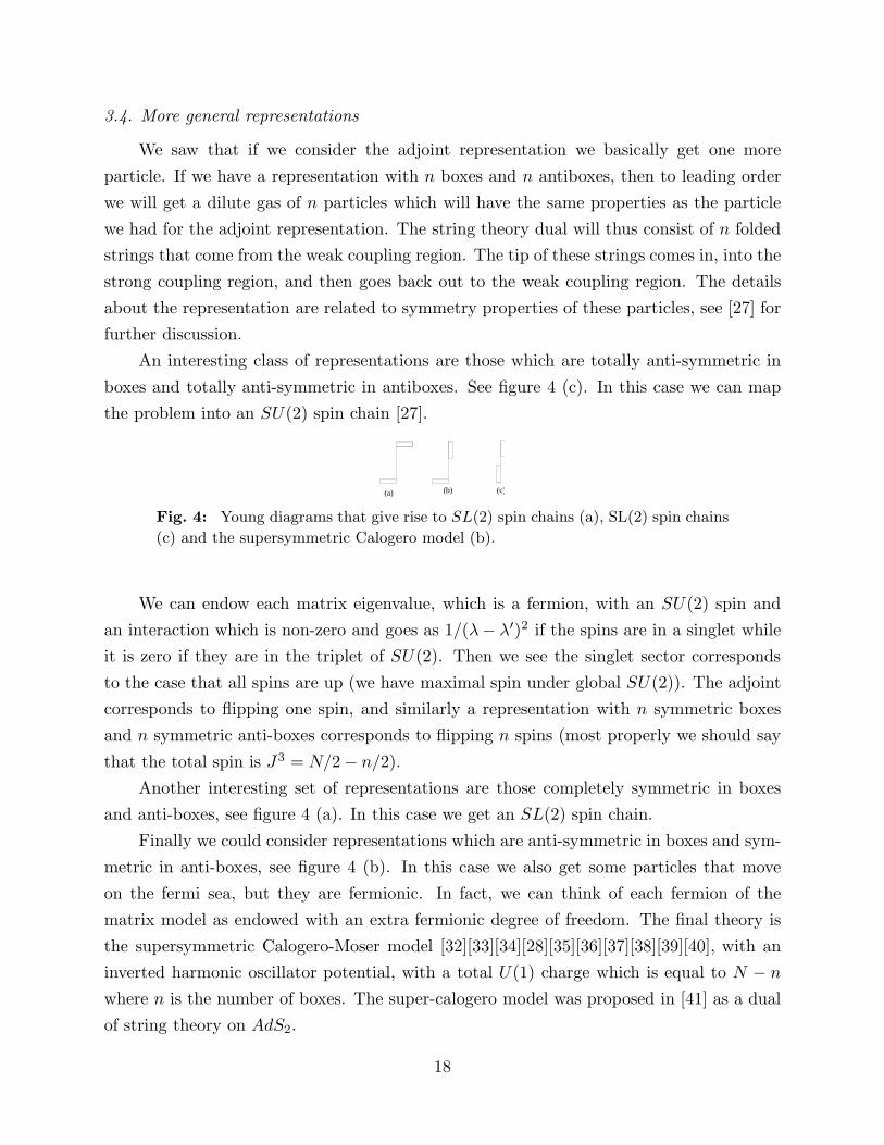
An interesting class of representations are those which are totally anti-symmetric in

boxes and totally anti-symmetric in antiboxes. See figure 4 (c). In this case we can map

the problem into an SU(2) spin chain [27].

(a) (b) (c)

Fig. 4: Young diagrams that give rise to SL(2) spin chains (a), SL(2) spin chains

(c) and the supersymmetric Calogero model (b).

We can endow each matrix eigenvalue, which is a fermion, with an SU(2) spin and

an interaction which is non-zero and goes as 1/(λ− λ′)2 if the spins are in a singlet while

it is zero if they are in the triplet of SU(2). Then we see the singlet sector corresponds

to the case that all spins are up (we have maximal spin under global SU(2)). The adjoint

corresponds to flipping one spin, and similarly a representation with n symmetric boxes

and n symmetric anti-boxes corresponds to flipping n spins (most properly we should say

that the total spin is J3 = N/2 − n/2).

Another interesting set of representations are those completely symmetric in boxes

and anti-boxes, see figure 4 (a). In this case we get an SL(2) spin chain.

Finally we could consider representations which are anti-symmetric in boxes and sym-

metric in anti-boxes, see figure 4 (b). In this case we also get some particles that move

on the fermi sea, but they are fermionic. In fact, we can think of each fermion of the

matrix model as endowed with an extra fermionic degree of freedom. The final theory is

the supersymmetric Calogero-Moser model [32][33][34][28][35][36][37][38][39][40], with an

inverted harmonic oscillator potential, with a total U(1) charge which is equal to N − n

where n is the number of boxes. The super-calogero model was proposed in [41] as a dual

of string theory on AdS2.

18

3.5. Two sided (or 0B) matrix model

In this subsection we consider a hermitian matrix model but we fill the two sides of

the inverted harmonic oscillator potential. This is also called the 0B matrix model, since

it is dual to type 0B string theory [42,43]. Since we are choosing α′ = 12 the matrix model

potential is exactly the same as in the bosonic string theory case. So, up to equation (3.6),

we have the same discussion as in the bosonic string case. The new feature is that we

need to consider both positive and negative values of λ. So we write λ = ±√2µ cosh τ on

these two sides. We also define the functions hl,r(τ) which are defined on the left and right

side of the inverted harmonic oscillator potential. Here we will assume that the Fermi

level is below the barrier. As in the bosonic case we extend the range of the functions

hl,r(−τ) = −hl,r(τ) for τ ≥ 0. Then the eigenvalue equations become

Ehr(τ) = − 1

π

∫ ∞

−∞dτ ′

[

hr(τ′)

4 sinh2 τ−τ ′

2

+hl(τ

′)

4 cosh2 τ−τ ′

2

]

+ v(τ)hr(τ) (3.27)

with

v(τ) ≡ 2

π(τmax − 1 − τ

tanh τ) (3.28)

We have a similar equation with r ↔ l. Due to the Z2 symmetry of the problem we can

define h+ and h− where h+ is such that hr(τ) = hl(τ) and h− is such that hr = −hl. The

two kinetic terms that appear in (3.27) can be diagonalized to

ǫh =K±h+ vh

K± =k

tanhπk∓ k

sinhπk= k

(

tanhπk

2

)±1

v = − 2

π

τ

tanh τ

ǫ =E − 2

π(τc − 1) = E +

2

πφc +

1

πlog µ+ const = ǫ+

1

πlogµ

(3.29)

where we have subtracted the divergent terms from the potential. We now see that the

divergent energy is twice what we had in the bosonic case, which is what we expect after we

identify√µeτ ∼ e−φ and use α′ = 1

2 . Note that the term involving logµ in the definition

of ǫ has a different coefficient than in the bosonic string because of the factor of two in

α′. In this units the Liouville cosmological constant term has the form µψψe2φ. As in

the bosonic case we were not able to solve the eigenvalue problem (3.29) directly. We

have checked, however, that in the two asymptotic limits ǫ → ±∞ the leading and first

subleading contributions computed from (3.29) match (2.21).

19

3.6. The vortex anti-vortex correlator for the superstring

In the type 0B superstring we have only one kind of winding string in the NS sector.

As in the bosonic string we can compute the two point function using the three point

function in [25]12. This gives

−∂µ〈e2(1−R)φe2(1−R)φ〉Liouv = i〈ψψe2φe2(1−R)φe2(1−R)φ〉Liouv

∼ iµ2R−1R2 Γ(−R)

Γ(R)

〈2pt〉 = − µ2RR2 Γ(−R)

Γ(R)

(3.30)

where the last line is the answer in the full string theory computation, including the

contribution due to the Euclidean time direction.

We can now consider the computation of the euclidean partition function for the 0B

matrix model in the adjoint representation. In this formula we will have to add over the

two separate phase shifts

Z0BW =

∫

dǫ∂ǫ(δ+(ǫ) + δ−(ǫ))

2πe−2πRǫ = −µ2R

∫ ∞

−∞dǫ

1

2ǫ(

1

tanhπǫ+ 1)e−2πRǫ =

= − 1

4 sin2 πRµ2R = −µ

2R

4π2R2Γ(−R)2Γ(R)2

(3.31)

We see that we get an answer that is essentially the same as the bosonic string (3.20), up

to the replacement µR → µ2R. Again, this is the proper normalization.

We can also reproduce the result (3.31) by considering the cylinder diagram between

two FZZT branes extended in time. This cylinder diagram comes purely from the exchange

of NS-NS closed strings only because these FZZT branes do not have RR charge in 0B.

This exchange has a form similar to (3.21) so the situation is very similar to what we

encountered in the bosonic case.

4. Non-singlets in the complex matrix model and 0A superstrings

Two dimensional 0A superstring theory was conjectured to be dual to a U(N) ×U(M) gauged matrix model, where the matrix M is in the (N, M) representation of the

12 It is the one called C3(αi) in [25].

20

gauge group [43]. In this section we consider the model in the presence of non-trivial

representations. So we can choose representations R, R of the two gauge groups and write

Z =

∫

DmDADAei∫

Tr[(D0m)†(D0m)+V (m†m)]TrRei∫

ATrRei∫

A (4.1)

In a gauge where we set A0 = 0 then we simply have a complex matrix model with

the requirement that we keep only the states which transform in representations R†, R†

under U(N) × U(M). Now we can ask which representations are allowed. We obviously

have that U(N) × U(M) ∼ U(1) × SU(N) × U(1) × SU(M). Clearly the representations

cannot transform under the overall U(1), so Q = −Q. In this paper we will consider

representations whose charges, including Q, Q, remain fixed as N → ∞. We will also keep

M −N finite13. In this case, we have that

Q = QN = −Q = −QM (4.2)

where QN and QM are the N-alities of the representations of SU(N) and SU(M) respec-

tively. If we keep the representations “fixed” when N → ∞ we can think of the N-alities

as well defined integers.

Using methods similar to the ones used to derive (3.2) we can derive the reduced

Hamiltonian for a complex matrix acting on wavefunctions that transform under represen-

tations R, R

H =

[

N∑

i=1

−1

2

∂2

∂ρi− 1

2ρ2

i +1

2

(Πii)

2 + (N −M)2 − 14

ρ2i

+

+ 2∑

i<j≤N

(ρ2i + ρ2

j)(Πi

j Π ji + Π i

j Π ji ) + 2ρiρj(Π

ij Π j

i + Π ij Π j

i )

(ρ2i − ρ2

j)2

+

+N∑

i=1

1

ρ2i

∑

j>N

(Π ij Π j

i + Π ji Π i

j )

P0

(4.3)

where P0 is a projector on the states obeying

Πii + Πi

i = 0 (no sum)

Π kl = 0 , l, k > N

(4.4)

where Πij are the U(N) generators and Πij are the U(M) generators. The last line implies

that under the decomposition SU(N) × SU(M − N) × U(1) ⊂ SU(M) we consider only

states that are trivial under SU(M −N). I have assumed that M ≥ N .

13 It is also interesting to consider the case when Q = −Q ∼ qN , which correspond to adding

a certain RR flux in the string theory. We consider this case in a separate publication [44].

21

4.1. Two simple examples of non-trivial representations

Consider N = M and pick a state in the adjoint of SU(N) and the trivial represen-

tation in U(M). So Π ji = 0. Then Πii = 0 (no sum) and the Hamiltonian becomes

H =∑

i

(

−1

2∂2

ρi− 1

2ρ2

i +1

2

(−14)

ρ2i

)

+ 2∑

i<j

ρ2i + ρ2

j

(ρ2i − ρ2

j)2Π j

i Π ij (4.5)

The term involving the one quarter is subleading at large µ, so I neglect it14. As in the

hermitian matrix model we can now write the eigenvalue problem as

Ew(λ) = 2

∫

dλ′ρ(λ′)λ2 + λ′2

(λ2 − λ′2)2(w(λ) − w(λ′)) (4.6)

We then use a formula similar to (3.6) to find a kinetic term and a potential which turns

out to be exactly the same as what we had for the 0B model. The crucial aspect is that

we can write

2λ2 + λ′

2

(λ2 − λ′2)2=

1

(λ− λ′)2+

1

(λ+ λ′)2(4.7)

So the problem is basically the same as the problem we had for the 0B case for the so

called even functions. We expect then that the scattering phase is given by δ+ in (2.19).

Obviously, we would get the same answer if we considered a representation which is trivial

in SU(N) and is the adjoint of SU(N).

Another interesting representation is a fundamental of the first and an anti-

fundamental of the second gauge group. Again we can label the states in the representation

by W ji . Then the constraint on the diagonal part forces W to be diagonal. We then find

an eigenvalue equation of the form

Ewi =1

2

1

λ2i

wi +wi

∑

j

(1

(λi − λj)2+

1

(λi + λj)2)−2

∑

j

(1

(λi − λj)2− 1

(λi + λj)2)wj (4.8)

where we used that4λλ′

(λ2 − λ′2)2=

1

(λ− λ′)2− 1

(λ+ λ′)2(4.9)

So we get a problem which is similar to the 0B problem for odd wavefunctions. The only

difference is a potential term which goes like 1/λ2. This term is subleading in the 1/µ

expansion, so we ignore it. In conclusion, we expect that the scattering phase is given by

δ− in (2.19).

14 It is not difficult to include it [43].

22

4.2. Partition functions and cylinder diagram for FZZT branes

Using the phase shifts, we can easily compute the partition functions for the ± cases.

We obtain

Z+ ∼∫

dǫ∂ǫδ+(ǫ)

2πe−2πǫ = −µ2R cos 2πR

2 sin2 2πR

Z− ∼∫

dǫ∂ǫδ−(ǫ)

2πe−2πǫ = −µ2R 1

2 sin2 2πR

(4.10)

Of course, Z+ + Z− gives us again (3.31).

Now let us consider the vortex anti-vortex correlator in 0A theory. Winding modes

can be in the NS-NS or RR sector. The NS-NS correlator was computed in (3.30). In

order to compute the RR correlator we consider the derivative with respect to µ of the

two point function. We then have to compute a three point function of one NS and two

RR vertex operators. We put the NS operator in the −1 picture and the RR operators in

the −1/2 picture. So we will need the super Liouville correlator in [25]15. We obtain

∂µ〈2pt〉 ∼ −Rµ2R−1 Γ( 12 −R)2

Γ( 12

+R)2

〈2pt〉 = − µ2R Γ( 12 −R)2

Γ( 12 +R)2

(4.11)

We can also compute the cylinder diagrams for FZZT branes in the 0A theory. In

the 0A case the FZZT branes carry RR charge. So the cylinder diagrams are a bit more

interesting than in the 0B case. The NS contribution is similar to that of the 0B theory,

and the bosonic theory. The RR contribution depends on the sign of η. For example, for

η = −1 we have

Zη=−1cyl =(2πR)

∑

n

∫

dE

(

cos2 2πEσ

sinh2 πE+

cos2 2πEσ

cosh2 πE

)

1

E2 + n2R2

Zη=−1cyl

∣

∣

∣

n=1∼−

(

1

sin2 πR− 1

cos2 πR

)

µ2Rµ−4RB

(4.12)

where in the second line we have extracted the contribution from the first pole at E = iR.

Similarly for the η = 1 brane we get

Zη=1cyl =(2πR)

∑

n

∫

dE

(

cos2 2πEσ

sinh2 πE− sin2 2πEσ

cosh2 πE

)

1

E2 + n2R2

Zη=1cyl

∣

∣

∣

n=1∼−

(

1

sin2 πR+

1

cos2 πR

)

µ2Rµ−4RB

(4.13)

15 It is the one called C3 in [25].

23

In the computation of the cylinder diagrams we did not keep track of the overall (positive)

numerical normalization. Up to this constant they agree with (4.10), after we identify

Z+ ∼ Zη=−1cyl |n=1 and Z− ∼ Zη=−1

cyl |n=1. The second term in (4.12)(4.13) comes from the

RR exchange and it has a form that is similar to (4.11).

ZZ FZZT+

−

+

− (a)

ZZ FZZT+

−

+

−(b)

η=−1

η=−1 η =1

η = −1

Fig. 5: Spectrum of open strings between ZZ branes and FZZT branes extended

in time in 0A. In (a) we see the spectrum between ZZ branes and FZZT branes

with the same η. In this case the ZZ and FZZT branes are charged under the

same gauge field. In (b) we consider an FZZT brane with opposite η. Here the

ZZ and FZZT branes are charged under a different gauge field. In both cases only

the region where the FZZT branes dissolve are charged. This region is represented

here as a dot, but it is not sharply localized in target space.

What these results are saying is that the open strings that stretch between the FZZT

and ZZ branes should have the following properties. See fig. 5. Let us set µ > 0. We have

ZZ branes with two possible charges. Let us consider the open strings stretching between

the ZZ branes and the FZZT branes with the same η as the ZZ branes. In this case we

expect that the open strings go between the FZZT brane and the ZZ brane of a given

charge, say plus. The charge they go to is related to the charge living at the tip of the

FZZT brane. Now let us consider the open strings between the ZZ and the FZZT brane

with the opposite η than the ZZ brane. We expect that the open strings end on the charge

plus or minus ZZ brane depending on their orientation. Notice that in this case the ZZ

and FZZT branes are charged under different spacetime gauge fields.

Could we see this properties directly from the string theory?. Let us think about

Liouville theory as a rational conformal field theory. Then according to the Cardy con-

struction the various branes are labeled by the primary fields. The two ZZ branes are

labeled by 1, ψ, depending on their RR charge. The FZZT branes with the same η as the

24

ZZ branes will be labeled by e(1+iσ)φ and ψe(1+iσ)φ. The open string spectrum is given

by taking the OPE of these fields. We see that this produces states that have the form

e(1+iσ)φ or ψe(1+iσ)φ. For generic σ only one of these two states is a superconformal pri-

mary. After restricting to superconformal primary states we see we have the open string

spectrum with the properties we sketched above. FZZT branes with the opposite η are

labeled by Ramond states of the form R±e(1+iσ)φ. In this case the OPE with the states

1, ψ will produce states of the form R±e(1+iσ)φ and R∓e

(1+iσ)φ. Again only half of these

states are superconformal primaries annihilated by the supercharge G0. When we include

X the surviving states will depend on the orientation of the string. This produces a string

spectrum which is consistent with the one we needed on the basis of the matrix model

answers.

5. Discussion

We studied the matrix model in its non-singlet sector. After subtracting a divergence

we saw that the matrix model hamiltonian is unbounded below in this sector. Nevertheless,

there are very natural Lorentzian computations which involve scattering amplitudes. These

amplitudes involve long strings in the target space. These are folded strings that stretch

from the weak coupling region. The tip of the string moves under the force provided by

the string tension. We considered in detail the case of the adjoint representation (and

also bifundamental, for 0A). In this case we have a single long string. More complicated

representations, whose Young diagrams involve n boxes and n anti-boxes, correspond to

states with n folded long strings. The string theory results match the matrix model results,

in the region where we could compute them explicitly.

This picture helps us understand the physical meaning of Euclidean computations

for winding correlators. In the matrix model these are often computed by appealing to

T-duality and then computing momentum correlators in the T-dual free fermion picture.

This helps us understand, for example, the sign of the two point function for winding

correlators.

Probably the picture of non-singlets proposed in this paper will be helpful for finding

a matrix model picture for the Lorentzian black hole. The action proposed in [2] for the

Euclidean black hole does not have an obvious local Lorentzian continuation. It is likely

that by taking a scaling limit with a large number of FZZT branes (3.23), we could find

a satisfactory lorentzian picture for the black hole. This point of view would suggest that

25

we should look for it as an excited long lived state in the non-singlet sector provided by

the FZZT branes in the limit (3.23).

Note that the mode that changes the value of the dilaton at the tip is not normalizable

in SU(2)k/U(1) for k < 3 (see section 7.3 of [45]). This implies that the thermodynamics

of the cigar is qualitatively different than in the large k situations, which was analyzed in

[46,47] 16. This fact explains that despite appearances we can actually change the radius

of the cigar in two dimensional string theory. It also explains why there is no sign of the

black hole in the singlet sector thermal partition function [48].

Acknowledgements

I would like to thank N. Seiberg for discussions and for collaboration on some of

the topics discussed. I also thank V. Kazakov, I. Kostov and D. Gaiotto for interesting

discussions and for showing me some of their unpublished work on this subject. I also

thank I. Klebanov and D. Kutasov for discussions on these issues.

This work was supported in part by DOE grant DE-FG02-90ER40542. I would also

like to thank the hospitality of the IHES, where part of this work was done.

Appendix A. Derivation of the scattering amplitudes

A.1. Bosonic string

We start by taking the b→ 1 limit of the formulas in [20]. The two point function for

the scattering of two open strings with two ends on the same D-brane is

〈e(1+iα)φe(1+iα)φ〉 =µ−iα Γ(2iα)G(1 − 2iα)G(1 + iα+ is)G(1 + iα)2

Γ(−2iα)G(1 + 2iα)G(1 − iα− is)G(1 − iα)2G(1 + iα− is)

G(1 − iα+ is)

coshπs =µB√µ

ig(α) ≡ logG(1 + iα)

G(1 − iα)= i

1

2

∫ ∞

0

dt

t

[

sin 2tα

sinh2 t− 2α

t

]

= −iπ∫ α

0

dα′ α′

tanhπα′

(A.1)

In the b→ 1 limit we also need to scale the bulk and boundary cosmological constants to

get a finite answer. In (A.1) we present the answer in terms of the rescaled variables. Note

that the function g(α) has the behavior

g(α) ∼ ∓π2α2 for α→ ±∞ (A.2)

16 In particular, section 6 of [2] does not seem to apply to the two dimensional black hole.

26

up to exponential corrections. We now take the scaling limit

s→ ∞ , α→ ∞ , ǫ ≡ α− 1

πlog 2µB = α− s− 1

2πlog µ = finite (A.3)

We see that the last factor in the first line in (A.1) is finite. There is also a finite contri-

bution from other terms. This arises because we want to write every α as α = s + ǫ and

then take the limit. Using (A.2) we find that the scattering amplitude is

eiδF ZZ =eiδ(ǫ)eiδdef (ǫ)eiδdiv(ǫ)

δ =g(ǫ+1

2πlogµ) − π

2(ǫ+

1

2πlog µ)2

δdef =1

π(φc + πǫ)2

δdiv = − 2φc(ǫ+1

πφc) +

4

πφc(log 2φc/π − 1) + 4ǫ log 2φc/π , φc ≡ log(2µB)

(A.4)

where the phase δdef is a phase that appears in the definition of the scattering phase

in (2.7). The first term in the divergent piece can be interpreted as coming from the

propagation from infinity to φc. The rest of the terms in the divergent amplitude seem

related to the details of the regularization procedure through the FZZT brane. In other

words, they are probably related to the particular way that the ends of the string interact

with the boundary Liouville potential. We can forget about the divergent piece. Notice

that the divergent pieces are independent of µ. This is a consistency check since all

these divergent pieces are related to our particular regularization of the amplitude using

FZZT branes and these branes are dissolving far away from the region where the Liouville

cosmological constant is important. After defining

δ(ǫ) ≡ g(ǫ) − π

2ǫ2 (A.5)

we recover (2.15).

In the limit when ǫ → −∞, then δ → 0 in agreement with (2.8). When ǫ → +∞ we

get

eiδeiπǫ2 ∼ µ−i(ǫ+ 14π

log µ) (A.6)

The energy dependence is the precisely the one we get for the scattering of a massless

“tachyon” from the Liouville potential. We have included a factor of eiπǫ2 which comes

from the difference between the definition of the scattering amplitude as in (2.7) versus the

more standard definition which would lack such factor. This more standard definition is

27

the one used to study the scattering of massless particles. We have chosen the apparently

more complicated definition (2.7) because with this definition the scattering phase depends

only on ǫ+ 12π

logµ. Had we chosen a more standard definition via

ψ ∼ e−i 12π

φ2+iǫφ + eiδusualei 12π

φ2−iǫφ (A.7)

then we would find that

δusual = δ + πǫ2 + π (A.8)

where δ is defined in (2.7). Notice that it is ǫ that appears here and not ǫ = ǫ+ 12π

logµ.

While δ depends only on ǫ, δusual in (A.8) depends on both ǫ, ǫ, but the dependence on

the latter is very simple.

A.2. Type 0 superstring

In order to compute the scattering amplitudes for the superstring we start with the

exact formulas of for the two point function in [25]. Again we just present the b→ 1 limit

of the formulas in [25]. Let us consider first the scattering of NS open strings which stretch

between FZZT branes with the same η. The result for the scattering of two such open

strings depends on η. Let us consider, for example, the amplitude for the scattering of

open strings on the η = −1 FZZT brane, in conventions where the ZZ brane has η = −1.

This gives17

〈e(1+iα)φe(1+iα)φ〉η=−1 =µ−iα G(1 − iα)2Γ(iα)

G(1 + iα)2Γ(−iα)

GNS(1 + iα+ 2is)

GNS(1 − iα− 2is)

G2NS(1 + iα)

G2NS(1 − iα)

×

× GNS(1 + iα− 2is)

GNS(1 − iα+ 2is)

GNS(x) =G(x

2)G(

x+ 1

2)

cosh πs =µB√µ

ig+(α) ≡ logGNS(1 + iα)

GNS(1 − iα)= ig(

α

2+i

2) + ig(

α

2− i

2)

= − i2

∫ α2

0

dα′α′π tanhα′π

(A.9)

17 Notice that 2φhere = φFukuda−Hosomichi in [25].

28

where G(x), and g(α) are the same functions as in (A.1). In these formulas α is equal to

the energy of the open string. Using the asymptotic behavior of gNS(α) as α → ±∞ we

can take the scaling limit

s→ ∞ , α→ ∞ , ǫ ≡ α− 2

πlog 2µB = (α− 2s− 2

2πlogµ) = finite (A.10)

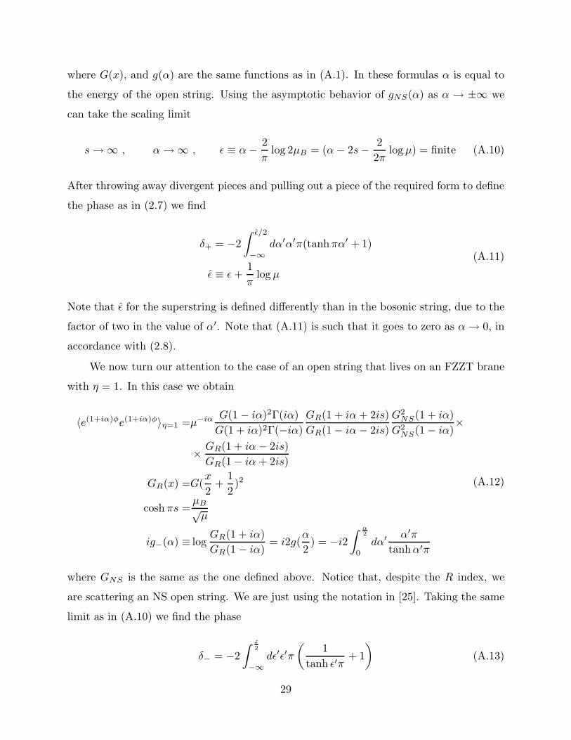
After throwing away divergent pieces and pulling out a piece of the required form to define

the phase as in (2.7) we find

δ+ = −2

∫ ǫ/2

−∞dα′α′π(tanhπα′ + 1)

ǫ ≡ ǫ+1

πlog µ

(A.11)

Note that ǫ for the superstring is defined differently than in the bosonic string, due to the

factor of two in the value of α′. Note that (A.11) is such that it goes to zero as α→ 0, in

accordance with (2.8).

We now turn our attention to the case of an open string that lives on an FZZT brane

with η = 1. In this case we obtain

〈e(1+iα)φe(1+iα)φ〉η=1 =µ−iα G(1 − iα)2Γ(iα)

G(1 + iα)2Γ(−iα)

GR(1 + iα+ 2is)

GR(1 − iα− 2is)

G2NS(1 + iα)

G2NS(1 − iα)

×

× GR(1 + iα− 2is)

GR(1 − iα+ 2is)

GR(x) =G(x

2+

1

2)2

coshπs =µB√µ

ig−(α) ≡ logGR(1 + iα)

GR(1 − iα)= i2g(

α

2) = −i2

∫ α2

0

dα′ α′π

tanhα′π

(A.12)

where GNS is the same as the one defined above. Notice that, despite the R index, we

are scattering an NS open string. We are just using the notation in [25]. Taking the same

limit as in (A.10) we find the phase

δ− = −2

∫ ǫ2

−∞dǫ′ǫ′π

(

1

tanh ǫ′π+ 1

)

(A.13)

29

Appendix B. Computation of matrix model reflection amplitudes

B.1. Derivation of (3.12)

We can rewrite (3.6) as

Eh(τ) = − 1

π

∫ ∞

0

dτ ′sinh τ sinh τ ′

(cosh τ − cosh τ ′)h(τ ′) + v(τ)h(τ)

v(τ) =1

π

∫ ∞

0

dτ ′sinh2 τ ′

(cosh τ − cosh τ ′)2

1 =1

π

∫ ∞

0

dτh(τ)2

(B.1)

It is possible to rewrite the kinetic term using

1

π

sinh τ sinh τ ′

(cosh τ − cosh τ ′)2=

1

π

1

4 sinh2 τ−τ ′

2

− 1

π

1

4 sinh2 τ+τ ′

2

(B.2)

Similarly the potential can be written as

v(τ) =1

π

(

τmax − 1 − τ

tanh τ

)

(B.3)

Since the eigenvalue distribution goes to zero at τ = 0 it is reasonable to assume that

h(τ = 0) = 0. Note that h(τ) is initially defined only for τ > 0. It is reasonable to extend

the definition of h(τ) on the whole real axis by defining it as an odd function of τ . Namely,

h(τ) = −h(−τ) for τ < 0. Then we can rewrite the kinetic term as an integral in τ ′ from

minus to plus infinity. In other words we find that

− 1

π

∫ ∞

0

dτ ′sinh τ sinh τ ′

(cosh τ − cosh τ ′)h(τ ′) = − 1

π

∫ ∞

−∞dτ ′

h(τ ′)

4 sinh2 τ−τ ′

2

(B.4)

We are then left with (3.12) (3.13).

B.2. Some scattering amplitudes from the matrix model

Let us discuss solutions of (3.12). Let us first assume that ǫ≪ 0. In this case we can

work in Fourier space and approximate the potential as τtanh τ ∼ τ = i∂k. Then we get the

equation

ǫh(k) =

(

k

tanhπk− i

1

π∂k

)

h(k) (B.5)

30

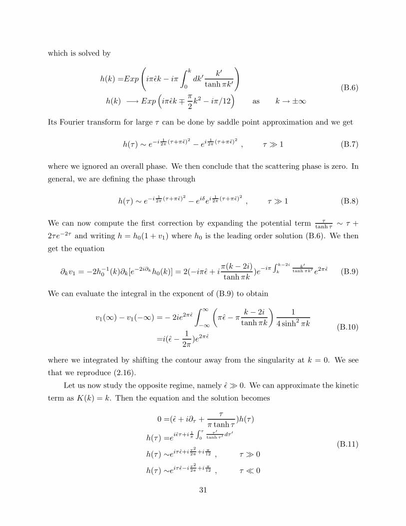
which is solved by

h(k) =Exp

(

iπǫk − iπ

∫ k

0

dk′k′

tanhπk′

)

h(k) −→ Exp(

iπǫk ∓ π

2k2 − iπ/12

)

as k → ±∞(B.6)

Its Fourier transform for large τ can be done by saddle point approximation and we get

h(τ) ∼ e−i 12π

(τ+πǫ)2 − ei 12π

(τ+πǫ)2 , τ ≫ 1 (B.7)

where we ignored an overall phase. We then conclude that the scattering phase is zero. In

general, we are defining the phase through

h(τ) ∼ e−i 12π

(τ+πǫ)2 − eiδei 12π

(τ+πǫ)2 , τ ≫ 1 (B.8)

We can now compute the first correction by expanding the potential term τtanh τ ∼ τ +

2τe−2τ and writing h = h0(1 + v1) where h0 is the leading order solution (B.6). We then

get the equation

∂kv1 = −2h−10 (k)∂k[e−2i∂kh0(k)] = 2(−iπǫ+ i

π(k − 2i)

tanhπk)e

−iπ∫

k−2i

k

k′

tanh πk′ e2πǫ (B.9)

We can evaluate the integral in the exponent of (B.9) to obtain

v1(∞) − v1(−∞) = − 2ie2πǫ

∫ ∞

−∞

(

πǫ− πk − 2i

tanhπk

)

1

4 sinh2 πk

=i(ǫ− 1

2π)e2πǫ

(B.10)

where we integrated by shifting the contour away from the singularity at k = 0. We see

that we reproduce (2.16).

Let us now study the opposite regime, namely ǫ≫ 0. We can approximate the kinetic

term as K(k) = k. Then the equation and the solution becomes

0 =(ǫ+ i∂τ +τ

π tanh τ)h(τ)

h(τ) =eiǫτ+i 1

π

∫

τ

0

τ′

tanh τ′ dτ ′

h(τ) ∼eiτ ǫ+i τ2

2π+i π

12 , τ ≫ 0

h(τ) ∼eiτ ǫ−i τ2

2π+i π

12 , τ ≪ 0

(B.11)

31

In order to solve the boundary conditions at the origin we still need to impose that h(τ) =

h(−τ). This can be done by taking h→ h(τ)−h(−τ) with h as defined above. Comparing

with (B.8) we see that the leading order phase is δ = −πǫ2 in agreement with the leading

order term in (2.17). Now we can do a first order expansion. We expand the kinetic term as

E(k) = k+2ke−2πk. The exponential is an operator performing a translation τ → τ +2πi.

As before we write h = h0(1 + v1) and we get

i∂τv1 = −2i∂τh0(τ + 2πi)

h0(τ)= 2(ǫ+

τ + 2πi

π tanh τ)e

i∫

τ+2πi

τ

τ′

π tanh τ′ dτ ′

e−2πǫ (B.12)

We can evaluate the integral in the exponent of (B.12) to obtain

v1(∞) − v1(−∞) = −ie−2πǫ

∫ ∞

−∞(ǫ+

τ + 2πi

π tanh τ)

1

2 sinh2 τ= i(ǫ+

1

2π)e−2πǫ (B.13)

where again we have shifted the contour to τ → τ + iπ. We see then that we reproduce

the subleading term in (2.16).

For the two sided matrix model we can also compute the leading terms and the

first correction. The whole computation is very similar to the one we did above, except

for factors of two. When we compute the first subleading correction starting from high

energies ǫ ≫ 0, then it is easy to see that the results for δ± differ by just a sign, as we

expect from the high energy expansion of (2.19) which is

δ− ∼− π

2ǫ2 + (ǫ+

1

π)e−πǫ , ǫ≫ 0

δ+ ∼− π

2ǫ2 − (ǫ+

1

π)e−πǫ , ǫ≫ 0

(B.14)

The difference in sign comes from the difference in sign when we expand the kinetic terms

in (3.29), K± ∼ k ∓ 2ke−πk.

For very low energies ǫ ≪ 0 we can do a similar expansion. Clearly for δ− we will

get a result similar to the one sided model, in agreement with (2.21). For δ+ the leading

correction will have the opposite sign which comes, basically, from the fact that we will

have a (coshπk/2)−2 instead of (sinhπk/2)−2 in an expression similar to (B.10). Going

through all the details one indeed finds the opposite sign, in agreement with (2.21).

In conclusion, we have checked explicitly that the leading and first subleading terms

computed in the matrix model agree with the string theory answers. This holds both for

the bosonic string and the superstring cases. It is interesting that the same functions are

appearing in the potential, the kinetic terms and the phase. This suggests that there must

be a simpler way to think about problem this that would allow us to get the answer more

quickly.

32

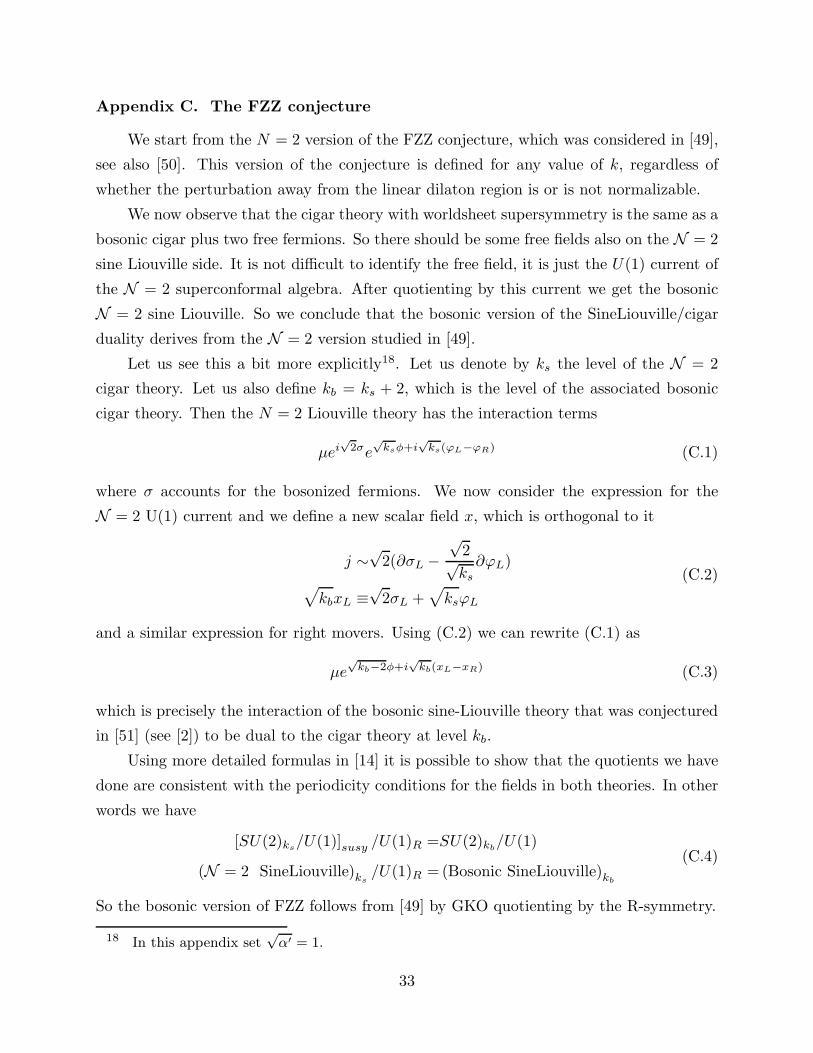
Appendix C. The FZZ conjecture

We start from the N = 2 version of the FZZ conjecture, which was considered in [49],

see also [50]. This version of the conjecture is defined for any value of k, regardless of

whether the perturbation away from the linear dilaton region is or is not normalizable.

We now observe that the cigar theory with worldsheet supersymmetry is the same as a

bosonic cigar plus two free fermions. So there should be some free fields also on the N = 2

sine Liouville side. It is not difficult to identify the free field, it is just the U(1) current of

the N = 2 superconformal algebra. After quotienting by this current we get the bosonic

N = 2 sine Liouville. So we conclude that the bosonic version of the SineLiouville/cigar

duality derives from the N = 2 version studied in [49].

Let us see this a bit more explicitly18. Let us denote by ks the level of the N = 2

cigar theory. Let us also define kb = ks + 2, which is the level of the associated bosonic

cigar theory. Then the N = 2 Liouville theory has the interaction terms

µei√

2σe√

ksφ+i√

ks(ϕL−ϕR) (C.1)

where σ accounts for the bosonized fermions. We now consider the expression for the

N = 2 U(1) current and we define a new scalar field x, which is orthogonal to it

j ∼√

2(∂σL −√

2√ks

∂ϕL)

√

kbxL ≡√

2σL +√

ksϕL

(C.2)

and a similar expression for right movers. Using (C.2) we can rewrite (C.1) as

µe√

kb−2φ+i√

kb(xL−xR) (C.3)

which is precisely the interaction of the bosonic sine-Liouville theory that was conjectured

in [51] (see [2]) to be dual to the cigar theory at level kb.

Using more detailed formulas in [14] it is possible to show that the quotients we have

done are consistent with the periodicity conditions for the fields in both theories. In other

words we have

[SU(2)ks/U(1)]susy /U(1)R =SU(2)kb

/U(1)

(N = 2 SineLiouville)ks/U(1)R = (Bosonic SineLiouville)kb

(C.4)

So the bosonic version of FZZ follows from [49] by GKO quotienting by the R-symmetry.

18 In this appendix set√

α′ = 1.

33

Appendix D. Computations of winding correlators via T-duality

Let us consider the problem of computing matrix model correlators in the singlet

sector. In the region of large λ the matrix model fermion reduces to a relativistic fermion.

Since we are at finite temperature this relativistic fermion lives on the circle. If we bosonize

this fermion we have a scalar field which is the tachyon. This is a free field in the asymptotic

region. We can think of this problem as a conformal field theory, given by the tachyon field

or the relativistic fermions, with a boundary. The boundary encodes the small λ region

and the reflection amplitudes for the fermions. In the fermion basis the boundary state

is very simple, we simply have a linear transformation between the left and right moving

fermion by a phase which is the scattering phase in the upside down harmonic oscillator

potential.

The correlators that we want to compute are most simply expressed by expanding

the tachyon field in momentum modes along the Euclidean time circle. In the asymptotic

region these can be expressed in terms of relativistic fermions. Again, it is convenient to

expand the fermions along the Euclidean time circle. These will have half integer moding

since the fermions are anti-periodic on the Euclidean time circle.

For example, if we are interested in the first momentum mode of the tachyon we write

it as

α−1|0〉 = ψ−1/2ψ−1/2|0〉 (D.1)

where |0〉 is the vacuum on the cylinder. We have similar formulas for the incoming and

outgoing tachyon modes corresponding to incoming or outgoing fermions. In the cylinder

incoming or outgoing fields are related to holomorphic or antiholomorphic fields and they

correspond to modes of the tachyon with positive or negative momentum on the circle [52].

So the computation boils down to an expression of the form

〈B|αin−1α

out−1 |0〉 (D.2)

The boundary state |B〉 encodes the reflection amplitudes for the fermions. These can be

expressed through the identities

〈B|(

ψin,s − iR−1(µ+ is/R)ψout,−s

)

= 0 , s ∈ Z +1

2

〈B|(

ψin,s − iR(µ− is/R)ψout,−s

)

= 0(D.3)

34

with the standard anticommutations relations

{ψs, ψs′} = δs+s′ (D.4)

for both in and out fields. The bounce factors are

R(E) =

√

Γ( 12 − iE)

Γ( 12 + iE)

(D.5)

for the bosonic string.

Using these formulas it is easy to compute the correlator in (D.2). We first express it

in terms of fermions through (D.1) and then use (D.3). The net result is

〈B|αin−1α

out−1 |0〉 = 〈B||0〉R(µ+ i

1

2R)R−1(µ− i

1

2R) (D.6)

The overlap 〈B|0〉 is defined to be the thermal partition function, as computed in [48].

In summary, (D.6) corresponds to the correlation function for the insertion of a tachyon

with momentum one and a tachyon with momentum minus one along the thermal circle.

After doing the T-duality, which corresponds to sending R→ 1/R and µ→ µR we obtain

the two point correlation function for a tachyon with winding number one and a tachyon

with winding number minus one. We identify this with the partition function of the matrix

model in the adjoint representations. In this fashion we have derived formula (3.25).

It is clear that we can use this method to compute more complicated correlators of

winding operators and hopefully it will be clear to the reader how to proceed.

In this way we could imagine computing the partition function in any representation.

All we would need to do is to express the representation in terms of the winding modes.

This can be done using the ideas in [53]. We will not go into the details because there is a

subtlety that gets in the way. If the decomposition involves modes with different winding

number, then the leg factors will be different for these different operators. Since we do not

understand the leg factors we cannot confidently assign a representation to a particular

configuration of winding correlators. In [54] this subtlety was ignored.

35

References

[1] I. Bars and D. Nemeschansky, “String Propagation In Backgrounds With Curved

Space-Time,” Nucl. Phys. B 348, 89 (1991). I. Bars, USC-91-HEP-B3. S. Elitzur,

A. Forge and E. Rabinovici, “Some global aspects of string compactifications,” Nucl.

Phys. B 359, 581 (1991). K. Bardacki, M. J. Crescimanno and E. Rabinovici,

“Parafermions From Coset Models,” Nucl. Phys. B 344, 344 (1990). M. Rocek,

K. Schoutens and A. Sevrin, “Off-shell WZW models in extended superspace,” Phys.

Lett. B 265, 303 (1991). G. Mandal, A. M. Sengupta and S. R. Wadia, “Classical solu-

tions of two-dimensional string theory,” Mod. Phys. Lett. A 6, 1685 (1991). E. Witten,

“On string theory and black holes,” Phys. Rev. D 44, 314 (1991).

[2] V. Kazakov, I. K. Kostov and D. Kutasov, “A matrix model for the two-dimensional

black hole,” Nucl. Phys. B 622, 141 (2002) [arXiv:hep-th/0101011].

[3] I. Klebanov, “String theory in two dimensions”, arXiv:hep-th/9108019; P. Ginsparg

and G. Moore, “Lectures on 2D gravity and 2D string theory”, arXiv:hep-th/9304011;

J. Polchinski, “What is string theory?,” arXiv:hep-th/9411028.

[4] G. W. Moore, “Gravitational phase transitions and the Sine-Gordon model,” arXiv:hep-

th/9203061.

[5] T. Suyama and P. Yi, “A holographic view on matrix model of black hole,” JHEP

0402, 017 (2004) [arXiv:hep-th/0401078].

[6] V. A. Kazakov and A. A. Tseytlin, “On free energy of 2-d black hole in bosonic string

theory,” JHEP 0106, 021 (2001) [arXiv:hep-th/0104138].

[7] J. L. Davis, L. A. Pando Zayas and D. Vaman, “On black hole thermodynamics of

2-D type 0A,” JHEP 0403, 007 (2004) [arXiv:hep-th/0402152].

[8] S. Alexandrov, “Matrix quantum mechanics and two-dimensional string theory in

non-trivial arXiv:hep-th/0311273.

[9] S. Y. Alexandrov and V. A. Kazakov, “Thermodynamics of 2D string theory,” JHEP

0301, 078 (2003) [arXiv:hep-th/0210251].

[10] S. Y. Alexandrov, V. A. Kazakov and I. K. Kostov, “Time-dependent backgrounds of

2D string theory,” Nucl. Phys. B 640, 119 (2002) [arXiv:hep-th/0205079].

[11] J. L. Davis and R. McNees, “Boundary counterterms and the thermodynamics of 2-D

black holes,” arXiv:hep-th/0411121.

[12] J. Park and T. Suyama, “Type 0A matrix model of black hole, integrability and

holography,” arXiv:hep-th/0411006.

[13] A. Sen, “Symmetries, conserved charges and (black) holes in two dimensional string

theory,” JHEP 0412, 053 (2004) [arXiv:hep-th/0408064].

[14] A. Giveon, A. Konechny, A. Pakman and A. Sever, “Type 0 strings in a 2-d black

hole,” JHEP 0310, 025 (2003) [arXiv:hep-th/0309056].

36

[15] S. Alexandrov, “Backgrounds of 2D string theory from matrix model,” arXiv:hep-

th/0303190.

[16] S. Alexandrov and V. Kazakov, “Correlators in 2D string theory with vortex conden-

sation,” Nucl. Phys. B 610, 77 (2001) [arXiv:hep-th/0104094].

[17] U. H. Danielsson, J. P. Gregory, M. E. Olsson, P. Rajan and M. Vonk, “Type 0A 2D

black hole thermodynamics and the deformed matrix model,” JHEP 0404, 065 (2004)

[arXiv:hep-th/0402192].

[18] W. A. Bardeen, I. Bars, A. J. Hanson and R. D. Peccei, “A Study Of The Longitudinal

Kink Modes Of The String,” Phys. Rev. D 13, 2364 (1976). W. A. Bardeen, I. Bars,

A. J. Hanson and R. D. Peccei, “Quantum Poincare Covariance Of The D = 2 String,”

Phys. Rev. D 14, 2193 (1976).

[19] I. Bars, “Folded strings,” arXiv:hep-th/9412044. I. Bars, “Folded strings in curved

space-time,” arXiv:hep-th/9411078. I. Bars and J. Schulze, “Folded strings falling

into a black hole,” Phys. Rev. D 51, 1854 (1995) [arXiv:hep-th/9405156].

[20] V. Fateev, A. B. Zamolodchikov and A. B. Zamolodchikov, “Boundary Liouville field

theory. I: Boundary state and boundary two-point function,” arXiv:hep-th/0001012.

[21] D. J. Gross and I. R. Klebanov, “Vortices And The Nonsinglet Sector Of The C = 1

Matrix Model,” Nucl. Phys. B 354, 459 (1991).

[22] D. Boulatov and V. Kazakov, “One-dimensional string theory with vortices as the

upside down matrix oscillator,” Int. J. Mod. Phys. A 8, 809 (1993) [arXiv:hep-

th/0012228].

[23] G. ’t Hooft, “A Two-Dimensional Model For Mesons,” Nucl. Phys. B 75, 461 (1974).

[24] J. Teschner, “Remarks on Liouville theory with boundary,” arXiv:hep-th/0009138.

[25] T. Fukuda and K. Hosomichi, “Super Liouville theory with boundary,” Nucl. Phys. B

635, 215 (2002) [arXiv:hep-th/0202032].

[26] G. Marchesini and E. Onofri, “Planar Limit For SU(N) Symmetric Quantum Dynam-

ical Systems,” J. Math. Phys. 21, 1103 (1980).

[27] J. A. Minahan and A. P. Polychronakos, “Interacting fermion systems from two-

dimensional QCD,” Phys. Lett. B 326, 288 (1994) [arXiv:hep-th/9309044]. J. A. Mi-

nahan and A. P. Polychronakos, “Integrable systems for particles with internal degrees

of freedom,” Phys. Lett. B 302, 265 (1993) [arXiv:hep-th/9206046]. J. A. Minahan and

A. P. Polychronakos, “Density correlation functions in Calogero-Sutherland models,”

Phys. Rev. B 50, 4236 (1994) [arXiv:hep-th/9404192].

[28] A. P. Polychronakos, “Generalized statistics in one dimension,” arXiv:hep-th/9902157.

[29] S. Dasgupta and T. Dasgupta, “Renormalization group approach to c = 1 matrix

model on a circle and D-brane decay,” arXiv:hep-th/0310106.

[30] A. B. Zamolodchikov and A. B. Zamolodchikov, “Structure constants and confor-

mal bootstrap in Liouville field theory,” Nucl. Phys. B 477, 577 (1996) [arXiv:hep-

th/9506136].

37

[31] G. W. Moore, M. R. Plesser and S. Ramgoolam, “Exact S matrix for 2-D string

theory,” Nucl. Phys. B 377, 143 (1992) [arXiv:hep-th/9111035].

[32] A. Dabholkar, “Fermions and nonperturbative supersymmetry breaking in the one-

dimensional superstring,” Nucl. Phys. B 368, 293 (1992).

[33] D. Z. Freedman and P. F. Mende, “An Exactly Solvable N Particle System In Super-

symmetric Quantum Mechanics,” Nucl. Phys. B 344, 317 (1990).

[34] L. Brink, T. H. Hansson, S. Konstein and M. A. Vasiliev, “The Calogero model:

Anyonic representation, fermionic extension and supersymmetry,” Nucl. Phys. B 401,

591 (1993) [arXiv:hep-th/9302023].

[35] E. Bergshoeff and M. A. Vasiliev, “The Calogero model and the Virasoro symmetry,”

Int. J. Mod. Phys. A 10, 3477 (1995) [arXiv:hep-th/9411093].

[36] P. Desrosiers, L. Lapointe and P. Mathieu, “Generalized Hermite polynomials in su-

perspace as eigenfunctions of the supersymmetric rational CMS model,” Nucl. Phys.

B 674, 615 (2003) [arXiv:hep-th/0305038]. P. Desrosiers, L. Lapointe and P. Math-

ieu, “Supersymmetric Calogero-Moser-Sutherland models: superintegrability structure

and eigenfunctions,” arXiv:hep-th/0210190.

[37] P. K. Ghosh, “Super-Calogero model with OSp(2|2) supersymmetry: Is the construc-

tion unique?,” Nucl. Phys. B 681, 359 (2004) [arXiv:hep-th/0309183].

[38] J. P. Rodrigues and A. J. van Tonder, “Marinari-Parisi and supersymmetric collective

field theory,” Int. J. Mod. Phys. A 8, 2517 (1993) [arXiv:hep-th/9204061].

[39] A. Jevicki and J. P. Rodrigues, “Supersymmetric collective field theory,” Phys. Lett.

B 268, 53 (1991).

[40] A. J. van Tonder, “A Continuum description of superCalogero models,” arXiv:hep-

th/9204034.

[41] H. Verlinde, “Superstrings on AdS(2) and superconformal matrix quantum mechan-

ics,” arXiv:hep-th/0403024.

[42] T. Takayanagi and N. Toumbas, “A matrix model dual of type 0B string theory in

two dimensions,” JHEP 0307, 064 (2003) [arXiv:hep-th/0307083].

[43] M. R. Douglas, I. R. Klebanov, D. Kutasov, J. Maldacena, E. Martinec and N. Seiberg,

“A new hat for the c = 1 matrix model,” arXiv:hep-th/0307195.

[44] J. Maldacena and N. Seiberg, in preparation.

[45] J. L. Karczmarek, J. Maldacena and A. Strominger, “Black hole non-formation in the

matrix model,” arXiv:hep-th/0411174.

[46] D. Kutasov and D. A. Sahakyan, “Comments on the thermodynamics of little string

theory,” JHEP 0102, 021 (2001) [arXiv:hep-th/0012258].

[47] M. Berkooz and M. Rozali, “Near Hagedorn dynamics of NS fivebranes, or a new

universality class of coiled strings,” JHEP 0005, 040 (2000) [arXiv:hep-th/0005047].

[48] D. J. Gross and I. R. Klebanov, “One-Dimensional String Theory On A Circle,” Nucl.

Phys. B 344, 475 (1990).

38

[49] K. Hori and A. Kapustin, “Duality of the fermionic 2d black hole and N = 2 Liouville

theory as mirror symmetry,” JHEP 0108, 045 (2001) [arXiv:hep-th/0104202].

[50] D. Tong, “Mirror mirror on the wall: On two-dimensional black holes and Liouville

theory,” JHEP 0304, 031 (2003) [arXiv:hep-th/0303151].

[51] L. Fateev, A. Zamolodchikov and Al. Zamolodchikov, unpublished notes.

[52] I. K. Kostov, “String equation for string theory on a circle,” Nucl. Phys. B 624, 146

(2002) [arXiv:hep-th/0107247]. S. Y. Alexandrov, V. A. Kazakov and I. K. Kostov,

“Time-dependent backgrounds of 2D string theory,” Nucl. Phys. B 640, 119 (2002)

[arXiv:hep-th/0205079]. I. K. Kostov, “Integrable flows in c = 1 string theory,” J. Phys.

A 36, 3153 (2003) [Annales Henri Poincare 4, S825 (2003)] [arXiv:hep-th/0208034].

M. Aganagic, R. Dijkgraaf, A. Klemm, M. Marino and C. Vafa, “Topological strings

and integrable hierarchies,” arXiv:hep-th/0312085.

[53] M. R. Douglas, “Conformal field theory techniques in large N Yang-Mills theory,”

arXiv:hep-th/9311130.

[54] J. Maldacena, Talk at strings 2004

39