Locating the orbits delineated by tidal streams

Mon. Not. R. Astron. Soc. 400, 548–560 (2009) doi:10.1111/j.1365-2966.2009.15494.x

Locating the orbits delineated by tidal streams

Andy Eyre and James BinneyRudolf Peierls Centre for Theoretical Physics, Keble Road, Oxford OX1 3NP

Accepted 2009 August 4. Received 2009 July 23; in original form 2009 May 13

ABSTRACTWe describe a technique that finds orbits through the Galaxy that are consistent with mea-surements of a tidal stream, taking into account the extent that tidal streams do not preciselydelineate orbits. We show that if accurate line-of-sight velocities are measured along a well-defined stream, the technique recovers the underlying orbit through the Galaxy and predictsthe distances and proper motions along the stream to high precision. As the error bars on thelocation and velocities of the stream grow, the technique is able to find more and more orbitsthat are consistent with the data and the uncertainties in the predicted distances and propermotions increase. With radial velocity data along a stream ∼40◦ long and �0.3◦ wide onthe sky accurate to ∼1 km s−1, the precisions of the distances and tangential velocities alongthe stream are 4 per cent and 5 km s−1, respectively. The technique can be used to diagnosethe Galactic potential: if circular speed curve is actually flat, both a Keplerian potential and�(r) ∝ r are readily excluded. Given the correct radial density profile for the dark halo, thehalo’s mass can be determined to a precision of 5 per cent.

Key words: stellar dynamics – methods: N-body simulations – Galaxy: kinematics anddynamics – Galaxy: structure.

1 IN T RO D U C T I O N

Deep optical surveys of the Milky Way and other Local Groupgalaxies have uncovered numerous stellar streams (Odenkirchenet al. 2001; Majewski et al. 2004; Belokurov et al. 2006; Ibata et al.2007). The Leiden–Argentine–Bonn survey of the Galaxy in the21 cm line of hydrogen (Kalberla et al. 2005) contains many similarstreams. In all probability, both stellar and gaseous streams havebeen tidally torn from orbiting bodies, and as such delineate theorbits of those bodies around the Galaxy (Johnston, Hernquist &Bolte 1996; Odenkirchen et al. 2003; Choi, Weinberg & Katz 2007).Newton’s laws of motion severely constrain the readily observablequantities along an orbit in the sky, namely the sequence of positionson the sky [l(u), b(u)] and the corresponding line-of-sight velocities,v‖(u), where u is a parameter that varies monotonically along thestream (Jin & Lynden-Bell 2007; Binney 2008, hereafter Paper I).In fact, if the observables are known to reasonable accuracy, datafor a single stream can strongly constrain the Galaxy’s gravitationalpotential, and once the potential is known, the distance and propermotion at each point on the stream can be predicted with an accuracythat far exceeds anything likely to be possible by conventionalastrometry (Paper I).

From the work of Paper I, it emerges that the major limitationon the diagnostic power of streams is that streams do not preciselydelineate individual orbits (Choi et al. 2007). This paper is devotedto exploring the extent to which this limitation can be overcome. InSection 2, we illustrate the extent of the problem; in Section 3, we

�E-mail: [email protected].

introduce significant improvements to the methodology of Paper Iand use these to identify orbits that are consistent with a given bodyof data. In Section 4, we test this approach. In Section 5, we examineour ability to correctly diagnose the Galactic potential. Section 6sums up and discusses directions for future work.

Except where stated otherwise, orbits and reconstructions arecalculated using the Galactic potential of Model II in Binney &Tremaine (2008), which is a slightly modified version of a halo-dominated potential described by Dehnen & Binney (1998a). Wetake the distance to the Galactic centre to be 8 kpc, and from Reid& Brunthaler (2004) (for V and W) and Dehnen & Binney (1998b)we take the velocity of the Sun in the Galactic rest frame to be (U ,V , W ) = (10.0, 241.0, 7.6) km s−1.

2 THE PROBLEM

The full curves in Fig. 1 show an orbit superficially similar to thatunderlying the Orphan Stream (Belokurov et al. 2007) from twoviewing locations – the position of the Sun and a position 120◦

further round the solar circle. Also shown in each projection are thelocations of particles tidally stripped from a self-gravitating N-bodymodel of a cluster launched onto the orbit given in Table 1. Clearly,the particles provide a very useful guide to the orbit of the cluster,but they do not precisely delineate it. Moreover, the relationshipof the orbit to the stream depends on viewing angle. The line-of-sight velocities of stream particles have a similar relationship tothe orbit’s line-of-sight velocity. Hence, even with perfectly error-free data, the orbit we seek will not coincide with the stream, andbefore we can fully exploit the dynamical potential of streams, we

C© 2009 The Authors. Journal compilation C© 2009 RAS

Locating the orbits delineated by tidal streams 549

Figure 1. Full (red) lines: the orbit of a progenitor of an Orphan-like stream. Broken (green/blue) lines: orbits of a star now seen at either end of the tidaltail. Points: particles tidally stripped from an N-body model of the Orphan-like progenitor. Upper panels: distributions on the sky; lower panels: line-of-sightvelocities. The N-body model had 60 000 particles set up as a King model with W = 2, r0 = 13.66 pc and M0 = 9381 M�, on the orbit detailed in Table 1,and evolved for 9.43 Gyr. The particles were advanced in time by the ‘FVFPS’ tree code of Londrillo, Nipoti & Ciotti (2003).

have to understand how to infer the location of an underlying orbitfrom measurements of the stream. For the moment, we assume thatthe errors in measured quantities are negligible, which in practicemeans that they are small compared to the intrinsic width of thestream. This condition will certainly be satisfied by sky coordinates.It will not always be satisfied by the velocity data, so we addressthe issue of velocity errors below.

With what precision could the track of an orbit be specified fromthe positions of the particles in Fig. 1? First, we need to be clearthat any orbit will do. Generally, it will be convenient to use theorbit that passes through some point that lies near the centre of theobserved stream, both on the sky and in line-of-sight velocity. Insome circumstances, this orbit will closely approximate the orbitof the centre of mass of the stream’s progenitor, but there is norequirement that this is so. Since a central point on the orbit ischosen at will, this point is associated with vanishing uncertainty.As one moves away from this point, either up or down the stream,it becomes more uncertain where the chosen orbit lies, and the sizeof the uncertainties must increase. Hence, the region of (l, b, v‖)

Table 1. Parameters of highlighted orbits from this paper. The coordinatesystem used is right-handed with x pointing away from the Galactic centreand y opposite the sense of Galactic rotation.

Orbit Position (x, y, z) (kpc) Velocity (x, y, z) (km s−1)

N-body Orphan (28.1, −10.0, 34.0) (−0.431, −0.179, −0.368)PD1 test orbit (35.5, 7.80, 37.8) (−0.0385, 0.272, 0.231)

space to which the orbit is confined by the observations is widest atits extremities and shrinks, usually to a point, at its centre. We callthis the ‘bow-tie region’.

In the top right-hand panel of Fig. 1, the leading and trailingstreams are not offset for most of the span, so we may assume thatthe orbit through the stream’s centre runs right down the centre of thestream. In the lower panels, the stream has a kink at the progenitorand our best guess is that the orbit through the point where the twohalves of the tail touch runs near the lower edge of the left-hand halfand near the upper edge of the right-hand half. In every case, theuncertainty in the location of the orbit grows from zero at the centreto roughly half width of the stream at its ends. Quantitatively, thelargest uncertainty is then 0.15◦ for the top left-hand panel, ∼0.25◦

for the top right-hand panel, and ∼5 km s−1 in the bottom panels.

3 ID E N T I F Y I N G DY NA M I C A L O R B I T S

Paper I showed that given an orbit’s projection on to the sky [l(u),b(u)] and the corresponding line-of-sight velocities v‖(u), the re-maining phase space coordinates can be recovered by solving thedifferential equations:

dt

du= 1

2F‖

⎛⎝ dv‖

du−

√(dv‖du

)2

− 4sF‖

⎞⎠,

ds

du= v‖

dt

du. (1)

C© 2009 The Authors. Journal compilation C© 2009 RAS, MNRAS 400, 548–560

550 A. Eyre and J. Binney

Here, u is distance on the sky down the projected orbit, s(u) isthree-dimensional distance to the orbit, t(u) is the time at whichthe orbiting body reaches the given point on the orbit and F ‖ is thecomponent of the Galaxy’s gravitational field along the line of sight.The reference frame used is the inertial frame in which the Galacticcentre is at rest; consequently, the velocities v‖ are obtained bysubtracting the projection of the Sun’s motion along the given lineof sight from the measured heliocentric velocities.

If the input data used to solve equations (1) are not derived froman orbit in the same force field as is used to derive F ‖, the recon-structed phase–space coordinates will not satisfy the equations ofmotion. Paper I observed that violation of the equations of motionsmight cause the reconstructed solution to violate energy conserva-tion, and therefore used rms energy variation down the track as adiagnostic for the quality of a solution. However, energy conser-vation is necessary but not sufficient to qualify a track as being anorbit. Here, we construct a diagnostic quantity from residual errorsin the equations of motion themselves, since orbits are defined tobe solutions of these equations.

We first derive the equations of motion. In the coordinates (s, b,l), the canonically conjugate momenta are

ps = s,

pb = s2b,

pl = s2 cos2 b l. (2)

The Hamiltonian is therefore

H = 1

2p2

s + 1

2

p2b

s2+ 1

2

p2l

s2 cos2 b+ �(s, b, l), (3)

and the equations of motion are

ps = s = p2b

s3+ p2

l

s3 cos2 b− ∂�

∂s,

pb = bs2 + 2bss = −p2l

s2

sin b

cos3 b− ∂�

∂b,

pl = s2 cos2 bl − 2s2 lb sin b cos b + 2ssl cos2 b = −∂�

∂l. (4)

As in Paper I, when solving equations (1) extensive use is madeof cubic spline fits to the data. In the examples presented in Paper I,natural splines were used in order to avoid specifying the gradient ofthe data at its endpoints. Significantly improved numerical accuracycan be achieved by taking the trouble to specify these gradientsexplicitly. Given the input data, we estimate the quantity dl/db atthe endpoints by fitting a quadratic curve through the first threeand last three points. dl/db is then computed at the location of themiddle point of each set, and the very first and very last points areconsidered ‘used’ and thrown away. This quantity is then used inthe geometric relation

du

db= ±

√1 + cos2 b

(dl

db

)2

, (5)

to compute db/du at the ends of the track. The sign ambiguity isresolved by inspection of the directionality of the input data. Wethen use the geometric relation

dl

du= ± sec b

√1 −

(db

du

)2

(6)

to obtain dl/du at the ends of the track, where the sign ambiguityis resolved in the same way. We are now able to fit cubic splinesthrough the input tracks, with the slopes at the end of the l(u) andb(u) tracks given as above, but at this stage the track of v‖(u) is

fitted with a natural spline. The reconstruction equations (1) arenow solved for t(u), which is then fitted by a cubic spline, with theslopes at the ends given explicitly by (1).

We can now compute l(t) and b(t) and fit splines to them, withthe slopes at the ends computed from dl/du and db/du by thechain rule. The momenta (2) are now calculated explicitly, usingthe derivatives of the splines l(t), b(t) in place of l, b. The slopes atthe endpoints, dv‖/du, can now be calculated from (4) and dt/du;the v‖(u) spline is refitted using these boundary conditions, thereconstruction repeated and the momenta recalculated.

The left- and right-hand sides of the equations of motion (4)are calculated explicitly. For each equation of motion, we define aresidual

R(t) = plhs(t) − prhs(t). (7)

These residuals are used to compute, for each equation of motion,the diagnostic quantity

D = log10

(∫ t2t1

dt R(t)2∫ t2t1

dt p2lhs

), (8)

where the residuals have been normalized by the mean-square ac-celeration and the times t1 and t2 correspond to the fifth and fifth-from-last input data points; the residual errors from the end regions,0 < t < t1 and t2 < t < tmax, tend to dominate the integratedquantity and are not easily reduced by modifying the input; they aretherefore excluded. The largest of the three values for D is used asthe diagnostic quantity for that particular input.

3.1 Parametrizing tracks

Our strategy for identifying a stream’s underlying orbit is to computethe diagnostic D (equation 8) for a large number of candidate tracks,and to find which candidates yield values of D consistent with theirbeing dynamical orbits.

We start by specifying a baseline track across the sky [lb(u′),bb(u′)], where u′ is a parameter that increases monotonically downthe track from −1 to 1. Similarly, we specify associated baselineline-of-sight velocities v‖b(u′). The baseline track is required tocome closer to every data point than the given uncertainty at thatpoint.

All candidate tracks should be smooth because orbits are. Wesatisfy this condition by expressing the difference between the base-line track and a candidate track as a low-order polynomial in u′. Forstreams that cover a wide range of longitudes, the parametrizationof candidate tracks is achieved by slightly changing the values of band v‖ associated with a given value of l from the values specifiedby the baseline functions. That is we write

b(u′) = bb(u′) +N∑

n=0

bnTn(u′),

v‖(u′) = v‖b(u′) +N∑

n=0

anTn(u′), (9)

where Tn is the nth order Chebyshev polynomial of the first kindand an and bn are free parameters. These 2N parameters are co-ordinates for the space of tracks that we have to search for orbits.When a stream does not stray far from the Galactic plane, candidatetracks are best parametrized by adjusting the baseline values of band v‖ at given longitude. In all examples in this paper, the series inequations (9) are truncated after N = 10. A larger number of termsallows the correction function to produce tracks that represent orbits



better, but makes the search procedure computationally more ex-pensive. The number of terms used is a compromise between theseconsiderations.

The space of tracks is defined by the an and bn and one extraparameter, the distance to the stream, s0, at the starting point u = 0for the integration of equations (1).

We shall henceforth denote a point in the (2N + 1)-dimensionalspace of parameters by χ . Each χ is associated with a completespecification of all six phase–space coordinates for every point onthe candidate orbit: l, b and v‖ follow from the parametrization andthe remaining coordinates are obtained by solution of the differentialequations (1). Consequently, each χ corresponds to a value of D(equation 8) that quantifies the extent to which the phase–spacecoordinates deviate from a dynamical orbit in the given potential.

3.2 Searching parameter space

Dynamical orbits are found by minimizing the sum

D′(χ ) = D(χ ) + p(χ ), (10)

where p(χ ) is the sum of the penalty functions:

p(χ ) =∑

i

pi,pos +∑

i

pi,vel + ps, (11)

where

pi,pos ={

�i,pos if �i,pos > 1

0 otherwise(12)

with

�i,pos = |b(li) − bb(li)|δb(li)

. (13)

Here, δbi is the width in b of the bow-tie region at li. Similarly,

pi,vel(l) ={

�i,vel if �i,vel > 1

0 otherwise(14)

with

�i,vel =∣∣v‖(li) − v‖b(li)

∣∣δv‖(li)

. (15)

Prior information about the distance to the stream is used by speci-fying the penalty function ps to be

ps ={

β |s0 − s0b| /δs if |s0 − s0b| > δs

0 otherwise,(16)

where δs is the half-width of the allowed range in the distance s0 tothe starting point of the integrations and s0b is the baseline value ofs0. These definitions are such that p(χ ) = 0 so long as the track lieswithin the region that is expected to contain the orbit, and rises tounity, or in the case of ps to β, on the boundary and then increasescontinuously as the orbit leaves the expected region.

In practical cases, the prior uncertainty in distance is large, andthe obvious way to search for orbits is to set δs to the large valuethat reflects this uncertainty and then set the algorithm describedbelow to work. It will find candidate orbits for certain distances.However, we shall see below that it is more instructive to searchthe range of possible distances by setting δs to a small value suchas 0.5 kpc and searching for orbits at each of a grid of values ofs0b. In this way, we not only find possible orbits, but we show thatno acceptable orbits exist outside a certain range of distances. Inthis procedure, the logic underlying δs is very different from thatunderlying δb and δv‖.

Since p(χ ) is added to the logarithm of the rms errors in theequations of motion and increases by an order of unity at the edgeof the bow-tie region, the algorithm effectively confines its searchto the bow-tie region, where p = 0. Thus, at this stage we donot discriminate against orbits that graze the edge of the bow-tieregion in favour of ones that run along its centre. Our focus at thisstage is on determining for which distances dynamical orbits can beconstructed that are compatible with the data. Once this has beenestablished, distances that lie outside some range can be excludedfrom further consideration.

The space of candidate tracks χ is 21-dimensional, so an ex-haustive search for minima of D′ (equation 10) is impractical. Fur-thermore, the landscape specified by D′ is complex. Some of thiscomplexity is physical; the space should contain continua of relatedorbits, and ideally D′ → −∞ at orbits. Hence, deep trenches shouldcriss-cross the space. Superimposed on this physical complexity isa level of numerical noise arising from numerical limitations in thecomputation of D′(χ ). The limitations include the use of finite stepsizes in the solution of equation (1) and the subsequent evaluationof D′(χ ), as well as the difficulty in representing a true orbital trackwith a collection of sparse input points interpolated with splines. Inpractice, numerical noise sets a lower limit on the returned valuesof D′(χ ).

On account of the complexity of the landscape that D′ defines,‘greedy’ optimization methods, which typically follow the path ofthe steepest descent, are not effective in locating minima. The taskeffectively becomes one of global minimization, which is a well-studied problem in optimization.

We have used the variant of the Metropolis ‘simulated annealing’algorithm described in Press et al. (2002), which uses a modifiedform of the downhill simplex algorithm. In the standard simplexalgorithm, the mean of the values of the objective function overthe vertices decreases every time the simplex deforms. In the Presset al. algorithm, the simplex has a non-vanishing probability ofdeforming to a configuration in which this mean is higher thanbefore. Consequently, the simplex has a chance of crawling uphillout of a local minimum. The probability that the simplex crawlsuphill is controlled by a ‘temperature’ variable T: when T is large,uphill moves are likely, and they become vanishingly rare as T →0. During annealing, the value of T is gradually lowered from aninitially high value towards zero.

One vertex of the initial simplex is some point χ guess and theremaining 2N + 1 vertices are obtained by incrementing each coor-dinate of χ guess in turn by a small amount. For the coefficients of T0,this increment is approximately the size of the allowed half widths,δs, δv and δb. Increments for coordinates representing coefficientsof higher order Tn are scaled as 1/n. The overall size of these in-crements is, therefore, set by the size of the region within whichwe believe the global minimum to lie. It is important to note that ineach generation of a simplex, the increments should independentlyhave equal chance of being added to or subtracted from the valuesof χ guess, so that no part of the parameter space is unfairly under-sampled. The algorithm makes tens of thousands of deformationsof the simplex while T is linearly reduced to zero.

This entire process is repeated some tens of times, after whichwe have a sample of local minima that are all obtained from χ guess.

We now update χ guess to the location of the lowest of the min-ima just found and initiate a new search. The entire process isrepeated until the value of the diagnostic function D′(χ ) hits afloor. When this floor lies higher than the numerical noise floor,the attempt to find an orbit that is consistent with the assumedinputs has been a failure and we infer that no such orbit exists.



When the floor coincides with the numerical noise floor, we con-clude that the corresponding χ specifies an orbit that is compatiblewith the inputs. An approximate value for the numerical noise floorfor a given problem may be obtained as follows: given input thatperfectly delineates an orbit in the potential in use, the value ofD′ returned at the correct distance is approximately the numericalnoise floor. Conclusive proof that a candidate track with a particularvalue of D′ is an orbit can be obtained by integrating the equa-tions of motion from the position and velocity of any point on thetrack and ensuring that the time integration essentially recovers thetrack.

On account of the stochastic nature of the algorithm, an attempt tofind a solution at a particular distance occasionally sticks at a highervalue of D′ than the underlying problem allows. This conditionis identified by scatter in the values of D′ reached on successiveattempts and by inconsistency of these values with the values of D′

achieved for nearby distances – the function underlying the minimais smooth (see for example Fig. 6, below). When the magnitude ofthis scatter is significant, one can only confidently declare an attemptto find an orbit a failure if the D′ achieved is consistently higherthan the noise floor by more than the scatter; since the diagnosticmeasure D′ quantifies the extent to which a candidate track satisfiesthe equations of motion, by definition, tracks with higher D′ thanthe noise floor plus scatter cannot represent orbits.

When the observational constraints are weak, we expect severalorbits to be compatible with them. In particular, we will be able tofind acceptable orbits for a range of initial distances s0. It is thereforeimportant, for any given input, to run the algorithm starting frommany different values of s0b with δs set to prevent the algorithmstraying far from the specified s0b. In this way, the full range ofallowable distances can be mapped out, and dynamical orbits foundfor each distance in that range. In the case of significant scatterabout the noise floor, the range of distances at which valid orbits arefound is the range within which solutions yield values of D′ smallerthan the noise floor plus scatter.

Similar degeneracies in the parameters controlling the astrometryand line-of-sight velocities are less of a concern because if we haveorbits that differ in these observables, we simply concentrate on theorbit that lies closest to the baseline track.

4 T E S T I N G TH E M E T H O D

To test this method, we used the N-body approximation to theOrphan Stream described in Fig. 1 and Table 1 as our raw data.Sets of points of (l, b) and (l, v‖) were selected by eye to liedown the middle of the stream. These sets were each fitted with alow-order polynomial to ensure smoothness, and these polynomialswere sampled at 30 points to produce the baseline input data b(l) andv‖(l). To each data set we attached uncertainties δb and δv‖, whichthrough the penalty functions ppos and pvel (equations 12 and 14)constrain the tracks that the Metropolis algorithm can try. Details ofthe resulting pseudo data sets are given below, and are summarizedin Table 2.

In one case, PD1, the above baseline input data were replaced bythose of a perfect orbit and δb and δv‖ set very narrow (6 arcsec and2 × 10−3 km s−1) in order to validate the reconstruction algorithm.

The uncertainty δb(l) takes the same value for all the remainingpseudo data sets because we assume that the astrometry is suffi-ciently precise for the uncertainty in position to be dominated bythe offset of the stream from an orbit. In all cases, δb has a max-imum value of 0.15◦ at the ends of the stream, falling linearly tozero at the position of the progenitor, consistent with the orbit of

Table 2. Configurations for tests of the method.

Set δv‖,max (km s−1) δv‖,min (km s−1) offset v‖ (km s−1)

PD1 2 × 10−3 2 × 10−3 0PD2 4 0 0PD3 6 2 0PD4 10 10 0PD5 6 2 2PD6 15 10.5 10PD7 4 0 0

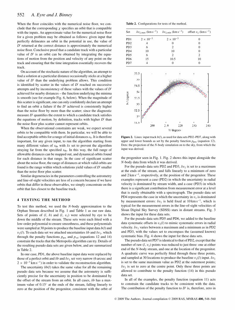
Figure 2. Lines: input track b(l), as used for data sets PD2–PD7, along withupper and lower bounds as set by the penalty function ppos (equation 12).Dots: the projection of the N-body simulation on to the sky, from which theinput was derived.

the progenitor seen in Fig. 1. Fig. 2 shows this input alongside theN-body data from which it was derived.

For the pseudo data sets PD2 and PD3, δv‖ is set to a maximumat the ends of the stream, and falls linearly to a minimum of zeroand 2 km s−1, respectively, at the position of the progenitor. Theseexamples represent a case (PD2) in which the uncertainty in radialvelocity is dominated by stream width, and a case (PD3) in whichthere is a significant contribution from measurement error at a levelthat is easily obtainable with a spectrograph. The pseudo data setPD4 represents the case in which the uncertainty in v‖ is dominatedby measurement errors: δv‖ is held fixed at 10 km s−1, which istypical for the measurement errors in the line-of-sight velocities ofSloan Digital Sky Survey (SDSS) stars in distant streams. Fig. 3shows the input for these data sets.

For the pseudo data sets PD5 and PD6, we added to the baselinedata systematic offsets in v‖(l) to mimic systematic errors in radialvelocity. δv‖ varies between a maximum and a minimum as in PD2and PD3, with the values set to encompass the (assumed known)systematic bias. Fig. 4 shows the input for these data sets.

The pseudo data set PD7 is identical to that of PD2, except that thenumber of raw (l, v‖) points was reduced to just three: one at eitherend of the N-body stream, and one at the location of the progenitor.A quadratic curve was perfectly fitted through these three points,and sampled at 30 locations to produce the baseline v‖(l) input. δv‖is set to the same maximum value as PD2 at the outermost points;δv‖ is set to zero at the centre point. Only these three points areallowed to contribute to the penalty function (14) in this pseudodata set.

In all of the examples, the penalty function (equation 11) actsto constrain the candidate tracks to be consistent with the data.The contribution of the penalty function to D′ is, therefore, zero in



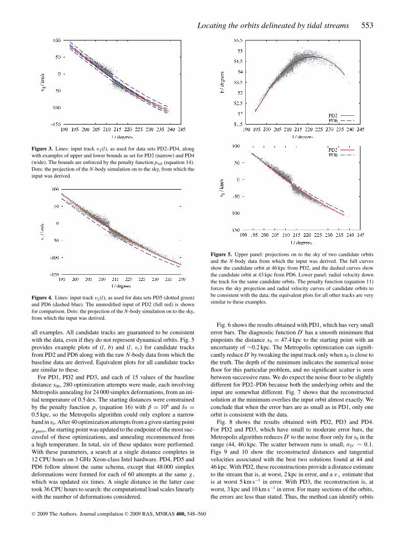
Figure 3. Lines: input track v‖(l), as used for data sets PD2–PD4, alongwith examples of upper and lower bounds as set for PD2 (narrow) and PD4(wide). The bounds are enforced by the penalty function pvel (equation 14).Dots: the projection of the N-body simulation on to the sky, from which theinput was derived.

Figure 4. Lines: input track v‖(l), as used for data sets PD5 (dotted green)and PD6 (dashed blue). The unmodified input of PD2 (full red) is shownfor comparison. Dots: the projection of the N-body simulation on to the sky,from which the input was derived.

all examples. All candidate tracks are guaranteed to be consistentwith the data, even if they do not represent dynamical orbits. Fig. 5provides example plots of (l, b) and (l, vr) for candidate tracksfrom PD2 and PD6 along with the raw N-body data from which thebaseline data are derived. Equivalent plots for all candidate tracksare similar to these.

For PD1, PD2 and PD3, and each of 15 values of the baselinedistance s0b, 280 optimization attempts were made, each involvingMetropolis annealing for 24 000 simplex deformations, from an ini-tial temperature of 0.5 dex. The starting distances were constrainedby the penalty function ps (equation 16) with β = 106 and δs =0.5 kpc, so the Metropolis algorithm could only explore a narrowband in s0. After 40 optimization attempts from a given starting pointχ guess, the starting point was updated to the endpoint of the most suc-cessful of these optimizations, and annealing recommenced froma high temperature. In total, six of these updates were performed.With these parameters, a search at a single distance completes in12 CPU hours on 3 GHz Xeon-class Intel hardware. PD4, PD5 andPD6 follow almost the same schema, except that 48 000 simplexdeformations were formed for each of 60 attempts at the same χ ,which was updated six times. A single distance in the latter casetook 36 CPU hours to search: the computational load scales linearlywith the number of deformations considered.

Figure 5. Upper panel: projections on to the sky of two candidate orbitsand the N-body data from which the input was derived. The full curvesshow the candidate orbit at 46 kpc from PD2, and the dashed curves showthe candidate orbit at 43 kpc from PD6. Lower panel: radial velocity downthe track for the same candidate orbits. The penalty function (equation 11)forces the sky projection and radial velocity curves of candidate orbits tobe consistent with the data; the equivalent plots for all other tracks are verysimilar to these examples.

Fig. 6 shows the results obtained with PD1, which has very smallerror bars. The diagnostic function D′ has a smooth minimum thatpinpoints the distance s0 = 47.4 kpc to the starting point with anuncertainty of ∼0.2 kpc. The Metropolis optimization can signifi-cantly reduce D′ by tweaking the input track only when s0 is close tothe truth. The depth of the minimum indicates the numerical noisefloor for this particular problem, and no significant scatter is seenbetween successive runs. We do expect the noise floor to be slightlydifferent for PD2–PD6 because both the underlying orbits and theinput are somewhat different. Fig. 7 shows that the reconstructedsolution at the minimum overlies the input orbit almost exactly. Weconclude that when the error bars are as small as in PD1, only oneorbit is consistent with the data.

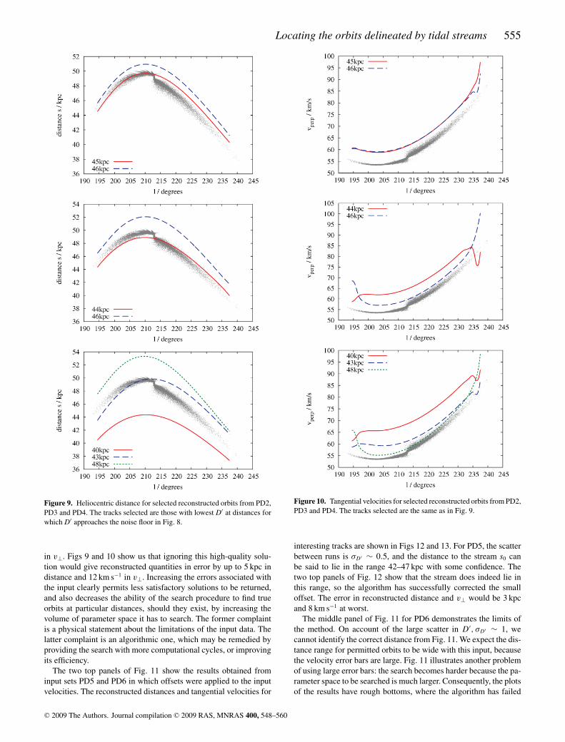
Fig. 8 shows the results obtained with PD2, PD3 and PD4.For PD2 and PD3, which have small to moderate error bars, theMetropolis algorithm reduces D′ to the noise floor only for s0 in therange (44, 46) kpc. The scatter between runs is small, σD′ ∼ 0.1.Figs 9 and 10 show the reconstructed distances and tangentialvelocities associated with the best two solutions found at 44 and46 kpc. With PD2, these reconstructions provide a distance estimateto the stream that is, at worst, 2 kpc in error, and a v⊥ estimate thatis at worst 5 km s−1 in error. With PD3, the reconstruction is, atworst, 3 kpc and 10 km s−1 in error. For many sections of the orbits,the errors are less than stated. Thus, the method can identify orbits



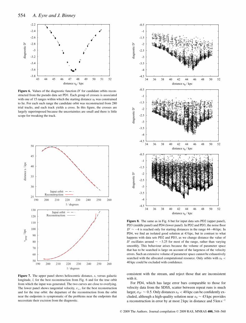
Figure 6. Values of the diagnostic function D′ for candidate orbits recon-structed from the pseudo data set PD1. Each group of crosses is associatedwith one of 15 ranges within which the starting distance s0 was constrainedto lie. For each such range the candidate orbit was reconstructed from 280trial tracks, and each track yields a cross. In this figure, the crosses arelargely superimposed because the uncertainties are small and there is littlescope for tweaking the track.

Figure 7. The upper panel shows heliocentric distance, s, versus galacticlongitude, l, for the best reconstruction from Fig. 6 and for the true orbitfrom which the input was generated. The two curves are close to overlying.The lower panel shows tangential velocity, v⊥, for the best reconstructionand for the true orbit: the departure of the reconstruction from the orbitnear the endpoints is symptomatic of the problems near the endpoints thatnecessitate their excision from the diagnostic.

Figure 8. The same as in Fig. 6 but for input data sets PD2 (upper panel),PD3 (middle panel) and PD4 (lower panel). In PD2 and PD3, the noise floorD′ ∼ −4 is reached only for starting distances in the range 44−46 kpc. InPD4, we find an isolated good solution at 43 kpc, but in contrast to whathappens with data sets PD2 and PD3, as we change distance the value ofD′ oscillates around ∼ −3.25 for most of the range, rather than varyingsmoothly. This behaviour arises because the volume of parameter spacethat has to be searched is large on account of the largeness of the velocityerrors. Such an extensive volume of parameter space cannot be exhaustivelysearched with the allocated computational resource. Only orbits with s0 <

40 kpc could be excluded with confidence.

consistent with the stream, and reject those that are inconsistentwith it.

For PD4, which has large error bars comparable to those forvelocity data from the SDSS, scatter between repeat runs is muchlarger, σD′ ∼ 0.5. Only distances s0 < 40 kpc can be confidently ex-cluded, although a high-quality solution near s0 ∼ 43 kpc providesa reconstruction in error by at most 2 kpc in distance and 5 km s−1



Figure 9. Heliocentric distance for selected reconstructed orbits from PD2,PD3 and PD4. The tracks selected are those with lowest D′ at distances forwhich D′ approaches the noise floor in Fig. 8.

in v⊥. Figs 9 and 10 show us that ignoring this high-quality solu-tion would give reconstructed quantities in error by up to 5 kpc indistance and 12 km s−1 in v⊥. Increasing the errors associated withthe input clearly permits less satisfactory solutions to be returned,and also decreases the ability of the search procedure to find trueorbits at particular distances, should they exist, by increasing thevolume of parameter space it has to search. The former complaintis a physical statement about the limitations of the input data. Thelatter complaint is an algorithmic one, which may be remedied byproviding the search with more computational cycles, or improvingits efficiency.

The two top panels of Fig. 11 show the results obtained frominput sets PD5 and PD6 in which offsets were applied to the inputvelocities. The reconstructed distances and tangential velocities for

Figure 10. Tangential velocities for selected reconstructed orbits from PD2,PD3 and PD4. The tracks selected are the same as in Fig. 9.

interesting tracks are shown in Figs 12 and 13. For PD5, the scatterbetween runs is σD′ ∼ 0.5, and the distance to the stream s0 canbe said to lie in the range 42–47 kpc with some confidence. Thetwo top panels of Fig. 12 show that the stream does indeed lie inthis range, so the algorithm has successfully corrected the smalloffset. The error in reconstructed distance and v⊥ would be 3 kpcand 8 km s−1 at worst.

The middle panel of Fig. 11 for PD6 demonstrates the limits ofthe method. On account of the large scatter in D′, σD′ ∼ 1, wecannot identify the correct distance from Fig. 11. We expect the dis-tance range for permitted orbits to be wide with this input, becausethe velocity error bars are large. Fig. 11 illustrates another problemof using large error bars: the search becomes harder because the pa-rameter space to be searched is much larger. Consequently, the plotsof the results have rough bottoms, where the algorithm has failed



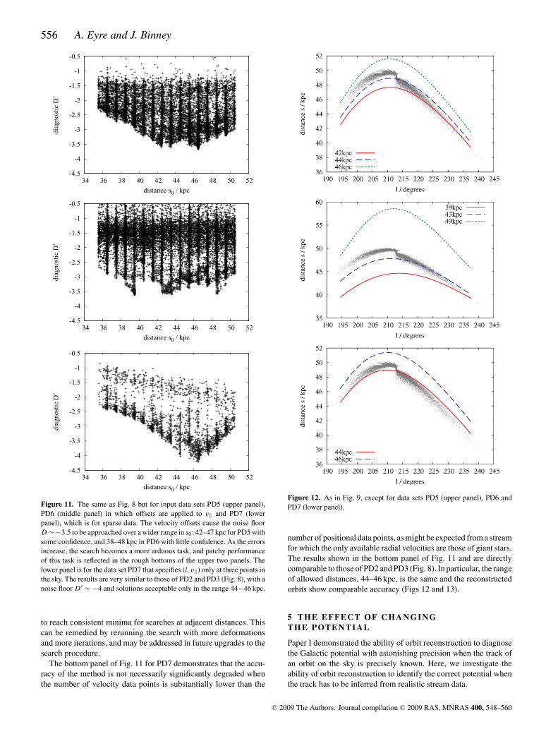
Figure 11. The same as Fig. 8 but for input data sets PD5 (upper panel),PD6 (middle panel) in which offsets are applied to v‖ and PD7 (lowerpanel), which is for sparse data. The velocity offsets cause the noise floorD ∼ −3.5 to be approached over a wider range in s0: 42–47 kpc for PD5 withsome confidence, and 38–48 kpc in PD6 with little confidence. As the errorsincrease, the search becomes a more arduous task, and patchy performanceof this task is reflected in the rough bottoms of the upper two panels. Thelower panel is for the data set PD7 that specifies (l, v‖) only at three points inthe sky. The results are very similar to those of PD2 and PD3 (Fig. 8), with anoise floor D′ ∼ −4 and solutions acceptable only in the range 44−46 kpc.

to reach consistent minima for searches at adjacent distances. Thiscan be remedied by rerunning the search with more deformationsand more iterations, and may be addressed in future upgrades to thesearch procedure.

The bottom panel of Fig. 11 for PD7 demonstrates that the accu-racy of the method is not necessarily significantly degraded whenthe number of velocity data points is substantially lower than the

Figure 12. As in Fig. 9, except for data sets PD5 (upper panel), PD6 andPD7 (lower panel).

number of positional data points, as might be expected from a streamfor which the only available radial velocities are those of giant stars.The results shown in the bottom panel of Fig. 11 and are directlycomparable to those of PD2 and PD3 (Fig. 8). In particular, the rangeof allowed distances, 44–46 kpc, is the same and the reconstructedorbits show comparable accuracy (Figs 12 and 13).

5 TH E E F F E C T O F C H A N G I N GTHE POTENTI AL

Paper I demonstrated the ability of orbit reconstruction to diagnosethe Galactic potential with astonishing precision when the track ofan orbit on the sky is precisely known. Here, we investigate theability of orbit reconstruction to identify the correct potential whenthe track has to be inferred from realistic stream data.



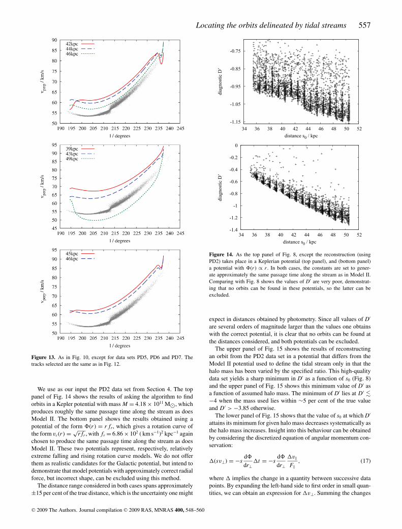
Figure 13. As in Fig. 10, except for data sets PD5, PD6 and PD7. Thetracks selected are the same as in Fig. 12.

We use as our input the PD2 data set from Section 4. The toppanel of Fig. 14 shows the results of asking the algorithm to findorbits in a Kepler potential with mass M = 4.18 × 1011 M�, whichproduces roughly the same passage time along the stream as doesModel II. The bottom panel shows the results obtained using apotential of the form �(r) = rfr, which gives a rotation curve ofthe form vc(r) = √

rfr , with fr = 6.86 × 102 ( km s−1)2 kpc−1 againchosen to produce the same passage time along the stream as doesModel II. These two potentials represent, respectively, relativelyextreme falling and rising rotation curve models. We do not offerthem as realistic candidates for the Galactic potential, but intend todemonstrate that model potentials with approximately correct radialforce, but incorrect shape, can be excluded using this method.

The distance range considered in both cases spans approximately±15 per cent of the true distance, which is the uncertainty one might

Figure 14. As the top panel of Fig. 8, except the reconstruction (usingPD2) takes place in a Keplerian potential (top panel), and (bottom panel)a potential with �(r) ∝ r . In both cases, the constants are set to gener-ate approximately the same passage time along the stream as in Model II.Comparing with Fig. 8 shows the values of D′ are very poor, demonstrat-ing that no orbits can be found in these potentials, so the latter can beexcluded.

expect in distances obtained by photometry. Since all values of D′

are several orders of magnitude larger than the values one obtainswith the correct potential, it is clear that no orbits can be found atthe distances considered, and both potentials can be excluded.

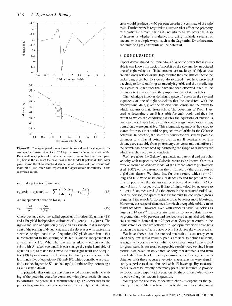
The upper panel of Fig. 15 shows the results of reconstructingan orbit from the PD2 data set in a potential that differs from theModel II potential used to define the tidal stream only in that thehalo mass has been varied by the specified ratio. This high-qualitydata set yields a sharp minimum in D′ as a function of s0 (Fig. 8)and the upper panel of Fig. 15 shows this minimum value of D′ asa function of assumed halo mass. The minimum of D′ lies at D′ �−4 when the mass used lies within ∼5 per cent of the true valueand D′ > −3.85 otherwise.

The lower panel of Fig. 15 shows that the value of s0 at which D′

attains its minimum for given halo mass decreases systematically asthe halo mass increases. Insight into this behaviour can be obtainedby considering the discretized equation of angular momentum con-servation:

�(sv⊥) = −sd�

dr⊥�t = −s

d�

dr⊥

�v‖F‖

, (17)

where � implies the change in a quantity between successive datapoints. By expanding the left-hand side to first order in small quan-tities, we can obtain an expression for �v⊥. Summing the changes



Figure 15. The upper panel shows the minimum value of the diagnostic forattempted reconstruction of the PD2 input versus the halo mass ratio of theDehnen–Binney potential in which the reconstruction has been attempted.M0 here is the value of the halo mass in the Model II potential. The lowerpanel shows the characteristic distance, s0, of the best solution versus halomass ratio. The error bars represent the approximate uncertainty in therecovered result.

in v⊥ along the track, we have

v⊥(end) − v⊥(start) = −∑ (

d�

dr⊥

�v‖F‖

+ v⊥�s

s

). (18)

An independent equation for v⊥ is

v⊥ = s�u

�t= sF‖

�u

�v‖, (19)

where we have used the radial equation of motion. Equations (18)and (19) yield independent estimates of v⊥(end) − v⊥(start). Theright-hand side of equation (18) yields an estimate that is indepen-dent of the scaling of � but systematically decreases with increasings, while the right-hand side of equation (19) yields an estimate thatis proportional to the scaling of �, but is almost independent ofs, since F ‖ ∝ 1/s. When the machine is asked to reconstruct theorbit with F ‖ taken too small, it can change the right-hand side ofequation (18) to match the new value of the right-hand side of equa-tion (19) by increasing s. In this way, the discrepancies between theleft-hand sides of equations (18) and (19), which contribute substan-tially to the diagnostic D′, can be largely eliminated by increasing sas � is scaled down.

In principle, this variation in reconstructed distance with the scal-ing of the potential could be combined with photometric distancesto constrain the potential. Unfortunately, Fig. 15 shows that in theparticular geometry under consideration, even a 10 per cent distance

error would produce a ∼50 per cent error in the estimate of the halomass. Further work is required to discover what effect the geometryof a particular stream has on its sensitivity to the potential. Alsoof interest is whether simultaneously using multiple streams, orstreams with multiple wraps (such as the Sagittarius Dwarf stream),can provide tight constraints on the potential.

6 C O N C L U S I O N S

Paper I demonstrated the tremendous diagnostic power that is avail-able if one knows the track of an orbit on the sky and the associatedline-of-sight velocities. Tidal streams are made up of objects thatare on closely related orbits. In particular, they roughly delineate theunderlying orbit, but they do not do so exactly. We have presenteda technique for identifying an underlying orbit and thus predictingthe dynamical quantities that have not been observed, such as thedistances to the stream and the proper motions of its particles.

The technique involves defining a space of tracks on the sky andsequences of line-of-sight velocities that are consistent with theobservational data, given the observational errors and the extent towhich streams deviate from orbits. The equations of Paper I areused to determine a candidate orbit for each track, and then theextent to which the candidate satisfies the equations of motion isquantified – in Paper I only violations of energy conservation alonga candidate were quantified. This diagnostic quantity is then used tosearch for tracks that could be projections of orbits in the Galacticpotential. In practice, the search is conducted for several possibledistances to a fiducial point on the stream. If constraints on thisdistance are available from photometry, the computational effort ofthe search can be reduced by narrowing the range of distances forwhich searches need to be conducted.

We have taken the Galaxy’s gravitational potential and the solarvelocity with respect to the Galactic centre to be known. Our testsrevolve around an N-body model of the Orphan Stream (Belokurovet al. 2007) on the assumption that it formed by the disruption ofa globular cluster. We show that for this stream, which is ∼40◦

long and 0.3◦ wide at its ends, distances to and tangential veloc-ities of points on the stream can be recovered to within ∼2 kpcand ∼5 km s−1, respectively, if line-of-sight velocities accurate to∼1 km s−1 are measured. As the errors in the measured radial ve-locities increase, the space of tracks that must be considered growsbigger and the search for acceptable orbits becomes more laborious.Moreover, the range of distances for which acceptable orbits can befound broadens. However, even with errors in radial velocities aslarge as ±10 km s−1, the uncertainties in the recovered distances areno greater than ∼10 per cent and the recovered tangential velocitiesare accurate to better than ∼20 per cent. Zero-point errors in theinput velocities that are reflected in appropriately wide error barsbroaden the range of acceptable orbits but do not skew the results.

We have shown that the method maintains its accuracy evenwhen very few radial velocity points are used to define the input,as might be necessary when radial velocities can only be measuredfor giant stars. In our tests, comparable results were obtained frompseudo data based on only three velocity measurements and frompseudo data based on 15 velocity measurements. Indeed, the resultsobtained with three accurate velocity measurements were signifi-cantly superior to those obtained with 15 lower quality measure-ments. Naturally, exactly how many points are required to providewell-determined input will depend on the shape of the radial veloc-ity curve along the stream in question.

We expect the accuracy of reconstructions to depend on the ge-ometry of the problem in hand. In particular, we expect streams at



apocentre, where families of orbits are compressed both on the skyand in radial velocity, to yield poorer results than streams away fromapocentre. Unfortunately, streams are most likely to be discoveredat apocentre because both orbital compression and low proper mo-tions around apocentre lead to a high density of stars at apocentre.We expect streams that are relatively narrow to produce more ac-curate results, because the permitted deviation of the orbit from thestream is then low. We also expect to have more difficulty recon-structing orbits from streams that contain a visible progenitor, sincethe potential of the progenitor will cause orbits in the progenitor’svicinity to differ materially from orbits in the Galaxy’s underlyingpotential.

Paper I suggested that it should be possible, if sufficiently accu-rate input is provided, to constrain the Galactic potential, since thewrong potential will not admit an acceptable orbit. We have testedthis possibility for input with realistic errors. We find that two poten-tials of significantly different shape, the Kepler potential and �(r) ∝r , are clearly excluded. We have also tested for changes in scalingof an otherwise correctly shaped potential, by varying the mass ofthe assumed dark halo around the value used to make the pseudodata. In this case, we find the correct potential is identified, withthe diagnostic quantity generally worsening as the halo mass movesaway from its correct value by more than ∼5 per cent. We furtherfind a consistent relationship between the reported stream distanceand the halo mass with which the reconstruction takes place. Al-though the reported distance is only weakly dependent upon halomass, this does open the possibility of using alternative distancemeasurements, such as photometric distances, in conjunction withthese techniques to constrain the Galactic potential. Further work isnecessary to determine a full scheme to recover parameters of thepotential from stream data. Also in question is the extent to whichsimultaneous reconstruction of multiple streams, and reconstructionof streams with multiple wraps around the Galaxy, might providestronger constraints on the Galactic potential than the short sectionof a single wrap that we have considered. It may also prove possibleto refine the other main assumption of our scheme, the location andvelocity of the Sun.

It is instructive to compare our method of finding orbits of progen-itors with the traditional N-body method. First, our method exploreseach orbit at a tiny fraction of the computational expense of N-bodymodelling, so it is feasible to automate the search of orbit space.Moreover, the search lends itself to parallelization. Whereas only asuccessful attempt to model a stream with N-bodies yields an inter-esting conclusion, our method can show that no orbit is consistentwith a given range of distances.

There are several directions in which this work could be profitablyextended.

(i) There is scope for a powerful synergy between our methodand N-body modelling: our method is first used to identify a likelyorbit and this orbit then provides initial conditions for an N-bodysimulation, which reveals the offset between the progenitor’s orbitand the stream. This knowledge would enable the bow-tie region tobe made narrower. Finally, our method is used again to determinethe orbit with still higher precision.

(ii) Currently, very long baseline interferometry observations ofmasers yield trigonometric parallaxes for the order of two dozensources located at several kpc from the Sun that are accurate toseveral per cent (Reid et al. 2009), and Gaia will yield results ofsimilar precision for several million stars. The method discussedhere promises distances of slightly higher precision to sources thatlie 50 to 100 kpc from the Sun. These ‘geometrodynamical’ dis-

tances in the terminology of Jin & Lynden-Bell (2007) may overtime play a significant role in astrophysics, just as trigonometricdistances did before them, by checking and calibrating photometricdistances. However, before this exciting prospect can be realized,we must overcome the problem that the method merely links dis-tances, velocities and the still uncertain gravitational potential ofthe Galaxy. How can we most effectively exploit this link betweenmeasurements of radial velocities, proper motions and photometryto obtain tight constraints on both the distances and the potential?This is an extremely important question given current interest inmapping the Galaxy’s dark matter through the gravitational forcefield that it generates. Undoubtedly, pinning down the potential willbe greatly facilitated by modelling several streams simultaneously.

(iii) Finer discrimination between candidate orbits would be pos-sible if one could lower the noise floor on the diagnostic functionD′ by upgrading the numerical methods used to obtain solutions ofequations (1). The scheme for searching the space of possible trackscould also be made faster and more reliable.

The list of streams to which this technique could be appliedis already quite long: obvious examples include the tidal tailsof the globular clusters Palomar 5 and NGC 5466, those of theLarge Magellanic Cloud, the Orphan Stream and the tidal streamof the Sagittarius dwarf galaxy. However, before we can exploitthe methods presented here, radial velocities are needed alongthese streams. The greatest precision is promised by the narrow-est streams, and these are well defined only in main-sequence stars.Therefore, the observational challenge is to obtain accurate radialvelocities for tens of faint stars. This will require 8-m telescope timefor what may seem unglamorous work. This paper suggests, how-ever, that the scientific rewards of such observations would be far-reaching.

Recently, it has been realized that orbits’ reconstruction is possi-ble using proper motions along the stream rather than radial veloci-ties (Eyre & Binney 2009). The principles developed in the presentpaper will undoubtedly transfer to orbit reconstructions from propermotions. It remains to be discovered whether they will enable use-ful distances to be determined from proper motions of currentlyattainable precision. We hope to report on this issue shortly.

AC K N OW L E D G M E N T S

AE acknowledges PPARC/STFC for partially funding this work,Carlo Nipoti for providing a copy of the FVFPS code, and JohnMagorrian for useful discussions about numerical methods. Wethank the anonymous referee for his/her suggestions.

REFERENCES

Belokurov V. et al., 2006, ApJ, 647, L111Belokurov V. et al., 2007, ApJ, 658, 337Binney J., 2008, MNRAS, 386, L47 (Paper I)Binney J., Tremaine S., 2008, Galactic Dynamics, 2nd ed. Princeton Univ.

Press PrincetonChoi J. H., Weinberg M. D., Katz N., 2007, MNRAS, 381, 987Dehnen W., Binney J., 1998a, MNRAS, 294, 429Dehnen W., Binney J., 1998b, MNRAS, 298, 387Eyre A., Binney J., 2009, MNRAS, in press (doi:10.1111/j.1745-

3933.2009.00744.x)Ibata R., Martin N. F., Irwin M., Chapman S., Ferguson A. M. N., Lewis

G. F., McConnachie A. W., 2007, ApJ, 671, 1591Jin S., Lynden-Bell D., 2007, MNRAS, 378, 64Johnston K. V., Hernquist L., Bolte M., 1996, ApJ, 465, 278



Kalberla P. M. W., Burton W. B., Hartmann Dap, Arnal E. M., Bajaja E.,Morras R., Poppel W. G. L., 2005, A&A, 440, 775

Londrillo P., Nipoti C., Ciotti L., 2003, Memorie Soc. Astron. Italiana,1, 18

Majewski S. R. et al., 2004, AJ, 128, 245Odenkirchen M. et al., 2001, ApJ, 548, L165Odenkirchen M. et al., 2003, AJ, 126, 2385

Press W. H., Flannery B. P., Teukolsky S. A., Vetterling W. T., 2002,Numerical Recipes in C. Cambridge Univ. Press, Cambridge

Reid M. J., Brunthaler A., 2004, ApJ, 616, 872Reid M. J. et al., 2009, ApJ, 700, 137

This paper has been typeset from a TEX/LATEX file prepared by the author.


Documents

Locating the orbits delineated by tidal streams