Embed Size (px)
Citation preview

Revista Colombiana de MatematicasVolumen 50(2016)2, paginas 211-276
Local unitary representations of the
braid group and their applications to
quantum computing
Colleen Delaney1,B, Eric C. Rowell2,Zhenghan Wang1,3
1University of California Santa Barbara, Santa Barbara, CA,U.S.A.
2Texas A&M University, College Station, TX, U.S.A.
3Microsoft Station Q, Santa Barbara, CA, U.S.A.
Abstract. We provide an elementary introduction to topological quantumcomputation based on the Jones representation of the braid group. We firstcover the Burau representation and Alexander polynomial. Then we discussthe Jones representation and Jones polynomial and their application to any-onic quantum computation. Finally we outline the approximation of the Jonespolynomial by a quantum computer and explicit localizations of braid grouprepresentations.
Key words and phrases. topological quantum computation, braid group repre-sentations, localizations, quantum algebra.
2010 Mathematics Subject Classification. 81P86, 20F36.
1. Introduction
Topological quantum computation is based on the storage and manipulation ofinformation in the representation spaces of the braid group, which consist ofquantum states of certain topological phases of matter [23]. The most impor-tant unitary braid group representations for topological quantum computationare the Jones representations [11], which are described by Temperley-Lieb-Jones theories. Temperley-Lieb Jones (TLJ) theories are the most ubiquitous
211

212 COLLEEN DELANEY, ERIC C. ROWELL & ZHENGHAN WANG
examples of unitary modular categories. The Jones-Wenzl projectors, or idem-potents, in TLJ theories can be used to model anyons, quasiparticle excitationsof a topological phase, like those believed to exist in fractional quantum Hall liq-uids. Hence the proper mathematical language to discuss topological quantumcomputation is unitary modular category (UMC) theory and the associatedtopological quantum field theory (TQFT). Both UMC and TQFT are highlytechnical subjects. However, the representations of the braid group from UMCsor TQFTs are a more accessible point of entry to the subject. These notes pro-vide an elementary introduction to some representations of the braid groupcoming from UMCs and TQFTs, and their application to topological quantumcomputation. We will use the braid group B∞ to mean the direct limit of alln-strand braid groups Bn for all n ≥ 1, where a representation of the braidgroup B∞ is a compatible sequence of representations of Bn.
Our focus is on the representations of the braid group discovered by Jonesin the study of von Neumann algebras [11]. Jones representations are unitary,which is important for our application to quantum computing. These repre-sentations also have a hidden locality and generically dense images. Unitarity,locality, and density are important ingredients for the two main theorems thatwe will present:
Theorem 1.1. The Jones representation of the braid group at q = e±2πi/r canbe used to construct a universal quantum computer for values of r not equal to1, 2, 3, 4, or 6.
Theorem 1.2. The Jones polynomial of oriented links at q = e±2πi/r can beapproximated by a quantum computer efficiently for any integer r ≥ 1.
While unitarity and density are easy to understand mathematically, localityis not formally defined in our notes as there are several interpretations, one ofwhich is discussed in Section 6. Essentially, a local representation of the braidgroup is one coming from a local TQFT, whose locality is encoded in thegluing formula. A first approximation of locality would mean a sequence ofrepresentations of Bn with a compatible Bratteli diagram of branching rules.
We motivate our study of the Jones representation and its quantum ap-plications with the Burau representation, which belongs to the classical world.The Burau representation leads to the link invariant called the Alexander poly-nomial, which can be computed in polynomial time on a classical computer.On the other hand, the link invariant corresponding to the Jones representa-tion, the Jones polynomial, is #P -hard to compute on a classical computer,but can be approximated by a quantum computer in polynomial time. Thisapproximation of quantum invariants by a quantum computer is realized bythe amplitudes of the physical processes of anyons, whose worldlines includebraids.
The contents of these notes are as follows. In section 2, we cover the Buraurepresentation and Alexander polynomial. In section 3, we discuss the Jones
Volumen 50, Numero 2, Ano 2016

BRAID GROUP REPRESENTATIONS AND TOPOLOGICAL QUANTUM COMPUTATION213
representation and Jones polynomial. Section 4 discusses anyons and anyonicquantum computation. In section 5, we explain the approximation of the Jonespolynomial by a quantum computer. Section 6 is on an explicit localization ofbraid group representations. While full details are not included, our presenta-tion is more or less self-contained with the exception of Thm. 4.21, which isimportant for addressing the issue of leakage. An elementary inductive argu-ment for Thm. 4.21 is possible and we will leave it to interested readers.
2. The Burau Representation and Alexander Polynomial
2.1. The braid group
The n-strand braid group Bn is given by the presentation
Bn =⟨σ1, σ2, . . . , σn−1
∣∣∣ σiσj = σjσi for |i− j| ≥ 2
σiσi+1σi = σi+1σiσi+1 for i = 1, 2, . . . , n− 1
⟩.
The first type of relation is known as far commutativity and the second is thebraid relation. Using the braid relation, one can check that all of the generatorsof the n-strand braid group lie in the same conjugacy class. Therefore, each n-strand braid group Bn is generated by a single conjugacy class when n ≥ 3.
The names of the relations are inspired by the geometric presentation of thebraid group, in which we picture braids on n “strands”, and the braid generatorsσi correspond to crossing the ith strand over the i + 1 strand. Multiplicationbb′ of two braid diagrams b and b′ is performed by stacking b′ on top of b andinterpreting the result as a new braid diagram.
For example, B3 = 〈σ1, σ2 | σ1σ2σ1 = σ2σ1σ2〉, where σ1 braids the firsttwo strands and σ2 the latter two.
σ1 = σ2 =
In these notes, we use the “right-handed convention” when drawing braid dia-grams of braid group generators, so that the overstrand goes from bottom leftto top right. As a result,
σ−11 =
Swapping the definitions of σ1 and σ−11 would give the “left-handed conven-
tion”.
In the picture presentation, far commutativity expresses the fact that whennonoverlapping sets of strands are braided, the result is independent of the
Revista Colombiana de Matematicas

214 COLLEEN DELANEY, ERIC C. ROWELL & ZHENGHAN WANG
order in which the strands were braided. The braid relation is given by
=
.
The braid relation is called the Yang-Baxter equation by some authors, but wewill reserve use of this phrase because, as will be explained shortly, there is asubtle difference between the two.
Another useful perspective is to identify Bn with the motion group (fun-damental group of the configuration space) of n points in the disk D2. Thenthe braid relation can be interpreted as saying that given three distinct pointson a line in the disk, if one exchanges the first and third points while keepingthe middle one stationary, then the braid trajectories are the same whether theexchange is performed in a clockwise or counterclockwise manner.
The braid group, denoted by B∞, is formed by taking the direct limit of then-strand braid groups with respect to the inclusion maps Bn ↪→ Bn+1 sendingσi 7→ σi. That is, we identify a braid word in Bn with the same braid word inBn+1. In pictures, this inclusion map Bn → Bn+1 adds a single strand after thebraid σ.
2.2. Representations of the Braid Group
For applications of braid group representations to quantum computing, thebraid group representations should be unitary and local. Moreover, for reasonsthat are not a priori clear, since the images of the braid generators σi willeventually be interpreted as quantum gates manipulating quantum bits, theyshould be of finite order and have algebraic matrix entries.
Recall that a matrix U is unitary if U†U = UU† = I. We denote by U(r)the group of r × r unitary matrices. A precise definition of locality requiresinterpreting the images of elements of the braid group as quantum gates, andis relegated to section 4 where quantum computation is discussed.
One important way to obtain representations of the braid group is to findsolutions to the Yang-Baxter equation.
2.2.1. The Yang-Baxter Equation and R-matrix
Let V be a finite dimensional complex vector space with a specified basis, andlet R : V ⊗ V → V ⊗ V be an invertible solution to the Yang-Baxter equation(YBE):
(R⊗ I)(I ⊗R)(R⊗ I) = (I ⊗R)(R⊗ I)(I ⊗R)
Volumen 50, Numero 2, Ano 2016

BRAID GROUP REPRESENTATIONS AND TOPOLOGICAL QUANTUM COMPUTATION215
where I is the identity transformation of V . We call such a solution to the YBEan R-matrix (as opposed to R-operator, since we have a basis with which towork).
Any R-matrix gives rise to a (local) representation of the braid group viathe identification
σi 7→ · · · R · · ·
For example, in the 3-strand braid group, we can take
σ1 7→ R = R⊗ idV
where R⊗ idV is a map from V ⊗ V ⊗ V to itself.
In general one considers a Yang-Baxter operator as having parameters thatindicate what pair of factors in V ⊗n it acts on: Ri,i+1 = Ii−1⊗Ri,i+1⊗ In−i−1.Then the Yang-Baxter equation is given by
Then the braid relation and Yang-Baxter equation differ by the choice ofindexing. In the former we keep track of the position of each strand, while inthe latter the labeling of the strands is fixed. For example, if we label the standas 1, 2, 3, the braid relation becomes
σ12σ13σ23 = σ23σ13σ12.
2.2.2. Locality and unitarity
The following R-matrix is a 4 × 4 solution to the Yang-Baxter equation forV = C2 with the standard basis and a ∈ C, and as such is local.
R =
a 0 0 0
0 0 a 0
0 a a− a3 0
0 0 0 a
If R is to be unitary, its columns must be orthonormal. In particular, a = a−1
and〈(0, 0, a, 0)T , (0, a, a− a3, 0)〉 = a(a− a3) = 0.
This implies that a4 = 1, whence the only possibilities for a are ±1 or ±i. Onecan check that each of these choices results in R being a unitary matrix.
While representations of the braid group arising from R-matrices are alwayslocal, unlike the example above they rarely unitary. There is a natural tensionbetween these two properties that make finding such a representation difficult.
Revista Colombiana de Matematicas

216 COLLEEN DELANEY, ERIC C. ROWELL & ZHENGHAN WANG
Conjeture 2.1. Any unitary R-matrix which has finite order and algebraicentries leads to a representation of the braid group with finite image.
It is in general difficult to find nontrivial solutions to the Yang-Baxter equa-tion. Historically, the theory of quantum groups was developed to address thisproblem, but solutions that arise from the theory of quantum groups are rarelyunitary. The state of the art is that for dimV = 1 and dimV = 2, all uni-tary solutions are known. While a classification for larger dimensions is yetunknown, there do exist nice examples of 4×4 and 9×9 unitary solutions [23].
These considerations make representations coming from solutions to theYang-Baxter equations unlikely candidates for applications to quantum com-putation. Next we consider the Burau representation.
2.3. The Burau representation of the braid group
There are two versions of the Burau representation: the unreduced representa-tion, which denoted by ρ, and the reduced representation, for which we reservethe notation ρ.
2.3.1. The unreduced Burau representation
There is a nice probabilistic interpretation of the unreduced Burau representa-tion that is due to Jones, which we will use as an introduction to the subject[12]. We start by defining the representation for positive braids, braids for whichall crossings are right-handed. More precisely, σ is positive if it can be writtenσ = σskik · · ·σ
sii1
where si > 0 for each i.
Imagine the braid diagram of a braid σ as a braided bowling alley with nlanes, where lanes cross over and under one another and at every overcrossingthere is a trap door that will open with probability 1− t when a ball rolls overit. Of course, due to gravity there is zero probability of a ball on a lower lanejumping up onto a lane crossing over it. Then starting from the bottom of thebraid and bowling down lane i, it ends up in lane j with some probability,which we can identify as the ijth entry of a matrix.
Then for positive braids the unreduced Burau representation ρ : Bn →GLn(Z[t, t−1]) can be defined by assigning each σ ∈ Bn to the matrix ρ(σ)given by
ρ(σ)ij =∑
paths p from i to j
w(p),
where w(p) is the probability corresponding to the path p, which is always ofthe form tk(1− t)l for some nonnegative integers k and l.
Volumen 50, Numero 2, Ano 2016

BRAID GROUP REPRESENTATIONS AND TOPOLOGICAL QUANTUM COMPUTATION217
For a concrete example, take the following braid, call it σ, in B4.
1 2 3 4
1 2 3 4
Note that the labels mark the relative position of the strands, as opposed tothe strands themselves. The matrix representing σ in GL4(Z[t, t−1]) is thengiven by
ρ(σ) =
1− t t(1− t) t2(1− t) t3
1 0 0 0
0 1 0 0
0 0 1 0
.
While the probabilistic interpretation only makes sense for positive braids, therepresentation of inverses of braid generators is already determined, for oncewe define the representation of a generator, for example
ρ( )
=
1− t t 0 0
1 0 0 0
0 0 1 0
0 0 0 1
,
using that ρ is a group homomorphism it follows that ρ(σ1)ρ(σ−11 ) = I. There-
fore the representation of the σ−11 must be given by the inverse of ρ(σ1) :
ρ( )
=
0 1 0 0
t 1− t 0 0
0 0 1 0
0 0 0 1
,
where t = 1/t. Thus left-handed crossings are assigned a factor of t for anovercrossing and 1 − t for an undercrossing. The remaining generators σi ofBn and their inverses can be represented by extending the construction in thenatural way. Then the representation of an arbitrary braid b = σskik · · ·σ
s1i1
isgiven by multiplying the representations of the constituent σij in the braidword. This defines the unreduced Burau representation of the braid group.
Revista Colombiana de Matematicas

218 COLLEEN DELANEY, ERIC C. ROWELL & ZHENGHAN WANG
As a fun example we introduce the following braid b = σ−13 σ2
2σ−13 σ−1
1 , oncedrawn by Gauss (see e.g. [5, Figure 2]).
The unreduced Burau representation of the Gauss braid is given by0 1 0 0
tt+ (1− t)2t t(1− t) + (1− t)2(1− t) 0 (1− t)t0 0 t (1− t)
t2(1− t) t(1− t)(1− t) (1− t)t (1− t)2 + tt
,
which has been left unsimplified to make the individual contributions frompaths more transparent.
The unreduced Burau representation of a braid b ∈ Bn has several propertiesworth mentioning.
(1) When t = 1, ρ(b) is a permutation matrix. This allows one to interpretρ(b) as a deformation of a permutation matrix.
(2) The representation ρ is reducible.
(3) There exists an invariant row vector (row eigenvector) of ρ(b), indepen-dent of b ∈ Bn.
The first property is clear from the construction of the unreduced Burau rep-resentation. The second and third properties are closely related, and we provethem below.
One of the nice aspects of the probabilistic interpretation of the Buraurepresentation is that it is an immediate consequence of the definition that theentries in each row of a matrix ρ(b) should sum to one, since probability mustbe conserved. Put another way,
ρ(σ)
1
1...
1
=
1
1...
1
.
That is, there is a one-dimensional subspace which is invariant under ρ(σ), forany σ ∈ Bn. Therefore the (unreduced) Burau representation is reducible, and
Volumen 50, Numero 2, Ano 2016

BRAID GROUP REPRESENTATIONS AND TOPOLOGICAL QUANTUM COMPUTATION219
we can obtain another representation by restricting to the orthogonal subspacespan{(1, 1, . . . , 1)}⊥. This is one way to define the reduced Burau representa-tion.
Since the determinant of a matrix is equal to the determinant of its trans-pose, if det(I − ρ(b)) = 0 for all b ∈ Bn, then
det((I − ρ(b))T ) = det(I − ρ(b)T ) = 0
for all b ∈ Bn. Then since ρ(b) has an eigenvector, ρ(b)T has an eigenvectorv with eigenvalue 1, ρ(b)T v = v for some v 6= 0. Taking the transpose of thismatrix equation, we find
vT ρ(b) = vT .
This shows that ρ(b) has an invariant row vector vT , proving the third property.In fact, this row vector takes the form
vT = (1, t, t2, . . . , tn−1).
Observing that
(1, . . . , 1, ti, ti+1, 1 . . . , 1)
Ii−1 0 0
0
(1− t t
1 0
)0
0 0 In−i−1
= (1, . . . , 1, ti − ti+1 + ti+1, ti+1, 1, . . . , 1),
it follows that vT defines an invariant row vector for the representations of thebraid group generators ρ(σi), and hence for all ρ(b), b ∈ Bn.
These facts can be used to prove properties of the Alexander polynomial, forwhich we need a more concrete definition of the reduced Burau representation.
2.3.2. The reduced Burau representation
An alternative approach to defining the reduced Burau representation yieldsan explicit basis.
We find a basis for an invariant subspace of ρ(Bn) by looking for eigenvaluesand eigenvectors of ρ(σi). We have seen already that (1, 1, . . . , 1)T is an eigen-vector with eigenvalue 1. One can check that another eigenvector correspondingto eigenvalue −t is given by (0, . . . , 0, −t︸︷︷︸
i
, 1︸︷︷︸i+1
, 0 . . . , 0)T .
Proposition 2.1. Let vi = (0, . . . , 0, −t︸︷︷︸i
, 1︸︷︷︸i+1
, 0 . . . , 0)T . Then span{v1, . . . , vn−1}
is an invariant subspace of ρ(b) for all b ∈ Bn.
Revista Colombiana de Matematicas

220 COLLEEN DELANEY, ERIC C. ROWELL & ZHENGHAN WANG
Proof. The image of each vi under ρ(b) can be written as a linear combinationof the vj .
ρ(σi)vi =
Ii−1 0 0
0
(1− t t
1 0
)0
0 0 In−i−1
=
0...
0
t2
−t0...
0
= −tvi
Similar calculations show
ρ(σi)vi−1 = vi−1+vt, ρ(σi)vi+1 = −tvi+vi+1, and ρ(σi)vj = vjwhen |j−i| ≥ 2.
This verifies that the subspace spanned by the vi is invariant, leading to thefollowing definition. �X
Definition 2.2. The reduced Burau representation ρ : Bn → GLn−1(Z[t, t−1])
is given by ρ(b) = ρ(b)∣∣∣span{vi}
.
2.3.3. Unitary Burau representations
Keeping in mind that we are looking for unitary representations of the braidgroup, it is natural to ask for which t ∈ C∗ the reduced Burau representationρ : Bn → GLn−1(Z[t, t−1]) is unitary.
One can check that the matrix representation corresponding to a braidgroup generator fails to be unitary for any choice of t. For example, consider
the braid with corresponding (unreduced) Burau matrix representation(1− t t
1 0
). Then either by direct computation or by noting that (since we
can safely ignore an overall phase factor of -1 without affecting unitarity) forno choice of t does this matrix admit the familiar parametrization of elements of
SU(2) as
(a b
−b a
)where a, b ∈ C and |a|2 + |b|2 = 1. By extending this obser-
vation to generators of Bn, it follows that the unreduced Burau representationis never unitary.
However, the situation is not completely hopeless. We end with a theoremthat tells us how to obtain a unitary representation from the reduced Buraurepresentation.
Volumen 50, Numero 2, Ano 2016

BRAID GROUP REPRESENTATIONS AND TOPOLOGICAL QUANTUM COMPUTATION221
Theorem 2.3. Let t = s2 where s ∈ C∗, and define Pn−1 =
1 0 · · · 0
0 s...
. . ....
0 · · · sn−1
,
Jn−1 =
s+ s−1 −1 · · · 0
−1 s+ s−1 . . ....
.... . .
. . . −1
0 · · · −1 s+ s−1
, and ρs(b) = Pn−1ρ(b)(Pn−1)−1,
where ρ is the reduced Burau representation and b ∈ Bn.
Then ρs is unitary with respect to the Hermitian matrix Jn−1. That is,
(ρs(b))†Jn−1ρs(b) = Jn−1
Moreover, for those s ∈ C∗ for which Jn−1(s) can be written as Jn−1(s) =X†X for some matrix X, Xρs(b)X
−1 gives a unitary representation.
Exercise 2.4. Find all s such that Jn−1(s) can be written Jn−1(s) = X†X.
There remain basic questions about the Burau representation to which theanswers are not yet known.
Open problem 2.6. The Burau representation is faithful for n = 1, 2, 3, andis not faithful for n ≥ 5 [2]. What about when n = 4?
2.4. The Alexander polynomial
The reduced Burau representation of the braid group can be used to constructa link invariant called the Alexander polynomial. The existence of invariantswhich are both powerful and computable is essential to the classification ofany mathematical object. Of course, Nature conspires so that these two char-acteristics are often hard to satisfy simultaneously. We will see that while theAlexander polynomial is computable in polynomial time, it is not quite sensitiveenough to distinguish between certain types of knots.
2.4.1. From braids to links
There is a natural way to turn a braid into a link by identifying the top andbottom strands in an order-preserving manner. This operation is called a braidclosure.
For example, one can check that the closure of the Gauss braid is the connectsum of two Hopf links.
Revista Colombiana de Matematicas

222 COLLEEN DELANEY, ERIC C. ROWELL & ZHENGHAN WANG
2.4.2. The Markov moves
We consider two other operations on braids, conjugation and stabilization, alsoknown as the Markov moves of type I and type II, and show that performingeither type of operation on a braid does not change the link that is obtainedfrom the braid closure.
I. Let b, g ∈ Bn. Then conjugation of the braid b by the braid g is given bythe map Bn → Bn
b 7→ gbg−1.
One can see that b = gbg−1 through the diagram below.
b
g
g−1
· · ·
· · ·
· · · = g
g−1
b· · ·
· · ·
· · · = b· · ·
· · ·
· · ·
II. Let b ∈ Bn, and let Bn be embedded in Bn+1 in the standard way, byadding a rightmost strand. Then stabilization of the braid b is given by themap Bn → Bn+1
b 7→ bσ±1n .
That is, we add a rightmost n + 1st strand to b to identify it as a braid inBn+1, and then we braid its nth and n + 1st strands with either an over- or
under-crossing. Once again, the diagrammatic argument that b = bσn is clear.
b
· · ·
· · ·
· · · = b
· · ·
· · ·
· · ·
Volumen 50, Numero 2, Ano 2016

BRAID GROUP REPRESENTATIONS AND TOPOLOGICAL QUANTUM COMPUTATION223
This move introduces a twist in the braid closure, and hence can be undoneby a Reidemeister move of type 1, so it doesn’t change the link b. A similar
argument shows b = bσ−1n .
Not only does manipulating a braid by Markov moves preserve the topologyof the braid closure, but whenever two braid closures agree, their correspondingbraids can be related by a finite number of Markov moves.
Theorem 2.5 (Markov). Consider the map from the set of all braids to theset of all links given by
{Bn} → {links}
b 7→ b.
If b1 = b2 as links, then b1 and b2 are related by a finite number of moves oftype I or type II and their inverses.
It is easy to see that the map b → b fails to be injective. For the simplestpossible example, take the braid closure of σ1, which gives the unknot.
=
It is also true, although much less trivial to show, that the map is onto. Givenany link there exists a finite number of Reidemeister moves that manipulatesthe link until it is in the form of a closure of a braid.
The Markov theorem gives us a way to study links through braid repre-sentations, since any braid invariant that is also invariant under the Markovmoves can be improved to a link invariant.
2.4.3. The Alexander polynomial
In order for a quantity to be an invariant of links, it must be invariant underthe Markov moves of type I and II. From linear algebra, we know that similarmatrices have the same determinant. It follows that the determinant of therepresentation of a braid is invariant under conjugation.
Recall the reduced Burau representation ρ : Bn → GLn−1(Z[t, t−1]) anddefine the matrices M(b) = I − ρ(b) and M(b) = I − ρ(b), where I is theidentity matrix with appropriate dimensions in each equation.
Definition 2.6. For b ∈ Bn, the Alexander polynomial is given by
∆(b, t) =det(M(b))
1 + t+ · · · tn−1.
Revista Colombiana de Matematicas

224 COLLEEN DELANEY, ERIC C. ROWELL & ZHENGHAN WANG
This establishes the convention that the Alexander polynomial of the unknot
is 1, i.e. ∆( )
= 1 . We present some results from linear algebra that can
be combined to prove that the Alexander polynomial is a link invariant, andstate some of its properties.
Lemma 2.7. Suppose A is an n× n matrix with the property that there existsa column vector w = (wi)
T and a row vector u = (uj) satisfying
(1) Aw = 0,
(2) uA = 0,
(3) wi 6= 0, uj 6= 0 for all i, j.
That is, A annihilates w, A is annihilated by u, and the coordinates of w andu are all nonvanishing. Then
(−1)i+jdet(A(i, j))
uiwj
is independent of i and j, where A(i, j) denotes the i, jth minor of A, that is,the (n − 1) × (n − 1) matrix obtained by the deleting the ith row and the jthcolumn from A.
The matrix M satisfies the hypotheses of this lemma. Recall that ρ(b) hadeigenvector (1, . . . , 1)T with eigenvalue 1 and invariant row vector (1, t, t2, . . . , tn−1).If we choose w = (1, . . . , 1)T and u = (1, t, t2, . . . , tn−1), it follows that Mw = 0and uM = 0. Evidently the coordinates of both w and u are nonvanishing.While the details are omitted, this leads to the proof of the next lemma.
Lemma 2.8.det(M(b))
1 + t+ · · ·+ tn−1= det(M(1, 1)).
This result gives us the freedom to delete any row and column of the matrixM , whose determinant recovers the Alexander polynomial.
The proof that the Alexander polynomial is indeed a link invariant entailschecking the invariance of ∆(b, t) under Markov moves using the lemmas.
There exists an efficient classical algorithm to turn any link L into a braidclosure b. For a braid b ∈ Bn, the Burau representation matrix and its deter-minant can be computed in polynomial time in the number of strands n andthe number and m the number of elementary braids in b.
Theorem 2.9. The Alexander polynomial of a link can be computed in poly-nomial time by a Turing machine.
Volumen 50, Numero 2, Ano 2016

BRAID GROUP REPRESENTATIONS AND TOPOLOGICAL QUANTUM COMPUTATION225
Note that the size of the Burau representation matrix is only (n−1)×(n−1)for a braid in Bn. As a comparison, we will see later the sizes of the Jonesrepresentation matrices for braids in Bn grow as dn × dn for some numberd > 1 as n→∞.
2.4.4. The Alexander-Conway polynomial, writhe, and skein relation
Having introduced the Alexander polynomial, one can define a related linkinvariant - the Alexander-Conway polynomial - through a slight renormalizationand by introducing a quantity called the writhe of a braid.
Let b = σskik · · ·σs1i1∈ Bn. The writhe or braid exponent is given by e(b) =∑k
i=1 si. Taking z = t1/2− t−1/2, the Alexander-Conway polynomial is definedas
∆(b, z) = (−t1/2)n−e(b)−1∆(b, t).
Under this new parametrization the behavior of our knot invariant with respectto left versus right-handed crossing can be expressed in the elegant form of theskein relation.
∆
( )− ∆
( )= z ∆
( )
Exercise 2.10. Deduce the skein relation from the definition of the Alexander-Conway polynomial and Lemma 2.8.
3. The Jones Representation and Jones polynomial
In a manner analogous to how the Alexander polynomial is defined in terms ofthe Burau representation, another link invariant, the Jones polynomial, can bestudied alongside the Jones representation. Computing the Alexander polyno-mial is easy in the sense of complexity theory, since there exists a polynomialtime algorithm to compute it. On the other hand, assuming that P 6= NP ,that is, assuming the longstanding conjecture that the complexity classes cor-responding to polynomial time and nondeterministic polynomial time are dis-tinct, computing the Jones polynomial is hard in the sense that there does notexist a polynomial time algorithm.
In this section we introduce the necessary background material for con-structing the Jones representation of the braid group: the quantum integers,the Temperley-Lieb and Temperley-Lieb-Jones algebra, and the Temperley-Lieb category. Section 4 covers the application of the Jones representation toquantum computing.
Revista Colombiana de Matematicas

226 COLLEEN DELANEY, ERIC C. ROWELL & ZHENGHAN WANG
3.1. Quantum integers
We should conceptualize the quantum integers as deformations of the integersby q, which we can either think of as generic (a formal variable) or a specificelement of C∗.
Definition 3.1. 1 Let n ∈ Z. Then quantum n, denoted [n]q, is given by
[n]q =qn/2 − q−n/2
q1/2 − q−1/2.
For instance, [1]q = 1 and [2]q = q1/2 + q−1/2. It is an easy application ofL’Hopital’s rule to show that [n]q → n in the limit q → 1, recovering the inte-gers. This shows we can truly think of [n]q as some deformation of n. However,one must take special care when performing arithmetic with quantum inte-gers, since the familiar rules of arithmetic need not apply. However, there isone important relation from integer arithmetic that still holds, the “quantumdoubling” formula.
Proposition 3.2. [2][n] = [n+ 1] + [n− 1].
This identity will reappear once we have introduced the Temperley-Liebalgebra.
3.2. The Temperley-Lieb algebra TLn(A)
Our goal is to find braid group representations with properties that are usefulfor quantum computation. In particular we want to be able to identify elementsof the image of these representations with matrices. Towards this end we passthrough either the Temperley-Lieb algebra or the Temperley-Lieb-Jones algebra.To motivate the construction of the Temperley-Lieb algebras, we recall thefollowing theorem that dictates how the the group algebra for a finite group Gdecomposes into the irreducible representations of G [10].
Theorem 3.3. Let G be a finite group, and C[G] = {∑agg | ag ∈ C} be the
group algebra of G over C. Then
C[G] ∼=⊕i
(dimVi)Vi,
where the Vi are a complete set of representatives of the isomorphism classesof finite-dimensional irreducible representations of G.
1There are two conventions in the literature when defining the quantum integers, depend-ing on whether a factor of 1/2 appears in the exponents; quantum n is sometimes defined as
[n]q = qn−q−n
q−q−1 .
Volumen 50, Numero 2, Ano 2016
BRAID GROUP REPRESENTATIONS AND TOPOLOGICAL QUANTUM COMPUTATION227
To illustrate the theorem we recall the representation theory of S3. Thereare three irreducible representations: the trivial, sign, and permutation repre-sentations, say U,U ′, and V , respectively. Then C[S3] = U ⊕ U ′ ⊕ 2V . Hence,as an algebra, C[S3] decomposes as C⊕ C⊕M2(C).
While we can completely describe C[G] when G is finite, when G is infinite,as in the case of G = Bn, we don’t have the same luxury. In order to get ahandle on C[Bn] we pass to a finite-dimensional quotient. The first step in thisprocess is to construct the Hecke algebra.
3.2.1. The Hecke algebra Hn(q)
Hereafter we will work in one of two fields, C or Q(A), the latter of which weuse to denote the field of rational functions in the Kauffman variable A overC. When we are interested in the generic Temperley-Lieb algebra, we work inQ(A), while in general specialize to a choice of A in C. For now we use F todenote the field Q(A).
The elements of the braid group algebra F[Bn] = {∑agg | g ∈ Bn, ag ∈ F}
are called formal (or quantum) braids. To motivate what relations we shouldquotient out by, we record a few observations.
Recall the presentation of the braid group
Bn =⟨σ1, σ2, . . . , σn−1
∣∣∣ σiσj = σjσi for |i− j| ≥ 2
σiσi+1σi = σi+1σiσi+1 for i = 1, 2, . . . , n− 1
⟩.
Taking the quotient of Bn by the normal subgroup generated by the σ2i results
in a group isomorphic to Sn. Thus there is a surjection of the braid group ontothe symmetric group, and we have an exact sequence
1 −→ PBn −→ Bn −→ Sn −→ 1.
This implicitly defines PBn, the pure braid group on n-strands, which willbe revisited in Section 4. In particular, we can get a representation of thebraid group by precomposing with a representation of the symmetric group.However, such a representation will not encode all of the information aboutthe braid group that is needed for computation. Instead one must look forrepresentations which do not factor through Sn.
Consider the quotient of F[Bn] by quadratic relations σ2i = aσi + b, for
i = 1, . . . , n−1, where a and b are independent of i. Note however that a and bare not independent of one another, since we can rescale by setting σi = σi/a.Then the relation becomes
σi2 = σi + b/a2.
In other words, we can just take a = 1, so that the relation is parametrized byb. Taking the quotient of F[Bn] by this relation defines a Hecke algebra.
Revista Colombiana de Matematicas

228 COLLEEN DELANEY, ERIC C. ROWELL & ZHENGHAN WANG
Definition 3.4. The Hecke algebra Hn(A) is the quotient F[Bn]/I of the braidgroup algebra, where I is the ideal generated by σ2
i − (A − A−3)σi − A−2 fori = 1, . . . , n− 1.
A presentation on generators and relations of the Hecke algebra furtherelucidates its structure. Renormalizing via q = A−4, and defining a new set ofgenerators by gi = A−1σi, we can define
Hn(q) =
⟨g1, g2, . . . , gn−1
∣∣∣∣∣gigj = gjgi for |i− j| ≥ 2
gi+1gigi+1 = gigi+1gi
g2i = q−1gi + q
⟩.
Due to the Hecke relation g2i = q−1gi + q, Hn(q) (and hence Hn(A)) is finite-
dimensional.
3.2.2. A presentation of the Temperley-Lieb algebra on generators and relations
In order to obtain the Temperley-Lieb algebra, we must pass through one morequotient. Reparametrizing once again, rescaling the generators of Hn(q) bydefining ui = Aσi − A2 and d = −A2 − A−2 = −[2]q, the Hecke algebrarelations become the following.
• uiuj = ujui when |i− j| ≥ 2 (far commutativity)
• uiui+1ui − ui = ui−1uiui−1 − ui−1 (braid relation)
• u2i = dui (Hecke relation)
To obtain the Temperley-Lieb algebra, we set the braid relation above to 0, soimpose one additional relation:
• uiui±1ui = ui
Definition 3.5. The generic Temperley-Lieb algebra TLn(A) is the quotientof the Hecke algebra Hn(q)/I, where I is the ideal generated by uiui±1ui− ui.
The generic Temperley-Lieb algebra TLn(A) is semisimple (also called amulti-matrix algebra), a direct sum of matrix algebras Mni
(F). This is the factthat enables us to work with matrix representations of the braid group, which,if unitary, can be thought of physically as quantum gates. Understanding howTLn(A) decomposes into matrix algebras is the key to applying the Jonesrepresentation to quantum computation.
Theorem 3.6. If A is generic, then TLn(A) is semisimple. If A ∈ C∗, thenTLn(A) is not in general semisimple.
We will return to the semisimple structure of TLn(A) after introducing itspicture presentation, in which computations can be performed using a graphicalcalculus.
Volumen 50, Numero 2, Ano 2016

BRAID GROUP REPRESENTATIONS AND TOPOLOGICAL QUANTUM COMPUTATION229
3.2.3. A picture presentation of the Temperley-Lieb algebra
In the graphical calculus the variable d = −A2−A−2 previously defined in thecontext of the presentation of TLn(A) with generators and relations takes onan important role. The variable d is called the loop variable, for reasons thatwill soon be clear.
Definition 3.7. A diagram in TLn(A) is a square with n marked points onthe top edge and n marked points on the bottom edge, and these 2n boundarypoints are connected by non-intersecting smooth arcs. In addition, there maybe simple closed loops in the diagram.
An equivalent diagram can be obtained by multiplying by a factor of dfor each closed loop removed, and we say two diagrams are the same if theyare d-isotopic, that is, if they are isotopic and the boundary points are of therespective diagrams are paired in the same way.
An arbitrary element of TLn(A) is a formal sum of diagrams, where eachdiagram is a word in the generators ui. The diagram of ui has a “cup” on thetop edge connecting the ith and i + 1st marked points, and a “cap” on thebottom edge connecting the ith and i + 1st marked points. The jth markedpoint on the top edge is connected to the jth marked point on the bottom edgeby a “through strand”.
· · ·
u1
,· · ·
u2
, . . . ,· · ·
ui, . . . ,
· · · · · ·
un−1
Multiplication of diagrams is performed by vertical stacking followed by rescaling-if D1, D2 ∈ TLn(A), then D1 · D2 is given by stacking D2 on top of D1 andrescaling to a square.
D1
D2
The Temperley-Lieb relations, far commutativity, the braid relation, and theHecke relation, can all be verified using the graphical calculus. For example,the Hecke relation is illustrated by
u2i =
· · ·
· · ·
· · ·
· · ·
= dui.
Revista Colombiana de Matematicas

230 COLLEEN DELANEY, ERIC C. ROWELL & ZHENGHAN WANG
Exercise 3.8. Show that the generators ui satisfy far commutativity and thebraid relation.
Theorem 3.9. The diagrammatic algebra for TLn(A) is isomorphic to theabstract Temperley-Lieb algebra given by generators and relations.
The proof of this result is made difficult by the diagrammatic algebra beingdefined up to d-isotopy.
As a vector space, TLn(A) is generated by all the Temperley-Lieb diagramsin TLn(A), of which there are Catalan number cn = 1
n+1
(2nn
)many up to d-
isotopy. In order to prove that the set of Temperley-Lieb diagrams forms a basisof TLn(A) as a vector space, one must show that there are no linear relationsamong the diagrams. This can be done by introducing an inner product onTLn(A), defined through the Kauffman bracket and a map called the Markovtrace, which can be thought of as a “quantum” analogue of the braid closure.
3.2.4. The Kauffman bracket
To find finite dimensional representations of the braid group, we begin by look-ing for an algebra homomorphism from the braid group algebra to finite matrixalgebras,
ρ : F[Bn]→⊕i
Mni(F).
A finite dimensional representation of Bn is then obtained via the restrictionof ρ to the braid group, ρ
∣∣Bn
. The Kauffman bracket 〈·〉 : F[Bn]→ TLn(A) isan algebra homomorphism which we can think of as producing Temperley-Liebdiagrams from formal braids by resolving crossings in the braid group algebra.
i i+1
= A
i i+1
+ A−1
i i+1
In terms of braid group generators and Temperley-Lieb generators, the Kauff-man bracket is expressed by
σi = AI +A−1ui.
Volumen 50, Numero 2, Ano 2016

BRAID GROUP REPRESENTATIONS AND TOPOLOGICAL QUANTUM COMPUTATION231
3.2.5. The Markov trace
The Markov trace of a diagram is the map Tr: TLn(A) 7→ F that sends adiagram D to its tracial closure.
D
· · ·
· · ·
· · · = d # loops
This defines the Markov trace on a basis of diagrams of TLn(A), and by ex-tending linearly it is defined on all of TLn(A). From the trace one can definean inner product 〈·, ·〉 : TLn(A)× TLn(A)→ F given by
〈D1, D2〉 = Tr(D1D2).
where the bar over a diagram denotes the diagram obtained by reflecting acrossthe horizontal midline.
D =D
Now the question of whether the diagrams in TLn(A) are linearly independentcan be translated into the question of whether the Gram matrix (M)ij =〈Di, Dj〉 has determinant zero. M is a cn × cn matrix, where cn is the nthCatalan number. While the details are not provided here, it is possible toexpress the determinant of M in the closed form
det(M) =
n∏i=1
∆i(d)an,i
where an,i =(
2nn−i−2
)+(
2nn−i)− 2
(2n
n−i−1
)and ∆i(x) is the ith Chebyshev
polynomial of the second kind, defined recursively by ∆0 = 1,∆1 = x, and∆i+1 = x∆i −∆i−1.
Therefore generic Temperley-Lieb diagrams are linearly independent, butwhenever the loop variable d is a root of a Chebyshev polynomial appearing inthe determinant of the Gram matrix, there is some linear dependence amongthe Temperley-Lieb diagrams. The Chebyshev polynomials are related to thequantum integers, which we will see later.
3.3. The Jones polynomial
To motivate the form that the Jones polynomial takes, we investigate the prop-erties that would be needed for a quantity to give an invariant of a link. Given
Revista Colombiana de Matematicas

232 COLLEEN DELANEY, ERIC C. ROWELL & ZHENGHAN WANG
a braid b ∈ Bn, we can apply the Kauffman bracket 〈·〉 to resolve the cross-ings, resulting in a sum of 2n Temperley-Lieb diagrams. Then 〈b〉 ∈ TLn(A),and we can apply the Markov trace. Thus we can consider their compositionTr〈·〉 : Bn → {links}. For example,
Tr〈 〉 = A + A−1 = Ad2 +A−1d = −A3d
A similar computation shows that the Markov trace of the Kauffman bracketapplied to the left handed crossing evaluates to −A−3. However, if we calculatethe trace of the unknot, which is topologically equivalent to the closure of theright-handed crossed, the result is d. While Tr〈·〉 is too sensitive to providea knot invariant, it can be calibrated by multiplying a factor of (−A−3)e(b),where e(b) is the writhe of the braid b introduced in Section 2.
We are now ready to define the Jones polynomial2 of a link.
Definition 3.10. Let b ∈ Bn, and let L = b be the link obtained from thebraid closure of b. Then the Jones polynomial J(L, q) of L is given by
J(L, q) =(−A−3)e(b)Tr〈b〉
d.
The reason for the factor of d in the denominator is to set the convention thatthe Jones polynomial of the unknot be equal to 1. It is necessary to point outthe the Jones polynomial is not well defined if we try to evaluate at a generallink instead of a braid closure - in order to make sense of the Jones polynomialof a link, it must be oriented.
By the Markov theorem, we know that whenever two links arising frombraid closures are equal, they are related by a finite number of Markov moves.
Therefore, it must be verified that the Jones polynomial is invariant underthe Markov moves. An diagrammatic argument identical to that for demon-strating the invariance of the Alexander polynomial under the braid closurecan be given.
Let a, b ∈ Bn. Invariance under conjugation can be seen by sliding diagramsaround their tracial strands. The proof-by-picture is identical to that providedfor the proof of invariance of the Markov moves under braid closure, exceptone replaces the braid diagram b by a Temperley-Lieb diagram. Similarly ifa = bσ±1
n , then the diagrammatic proof of invariance under stabilization isanalogous to that for braids, except now we introduce a factor of −A∓3 tocorrect for the writhe introduced by σ±1
n .
2Technically J(L, q) is a Laurent polynomial in q1/2, but it is still referred to as a poly-nomial in the literature.
Volumen 50, Numero 2, Ano 2016

BRAID GROUP REPRESENTATIONS AND TOPOLOGICAL QUANTUM COMPUTATION233
3.3.1. Example: the Jones polynomial of the trefoil knot
We end this discussion of the Jones polynomial with a famous example - the
right-handed trefoil knot, σ31 .
There are three crossings, and hence 23 = 8 terms in the resolution 〈σ31〉. The
terms can be organized by a binary tree of depth 3, where each edge is labeledby a “+” or a “−” according to the term in the Kauffman bracket. We computethe “ – + –” term as an example.
= −A−3 · (A−1 ·A ·A−1) · d2
One can check that J(σ31 , q) = q+q3−q4. It turns out that the Jones polynomial
of the left-handed trefoil knot is different. This is an improvement over theAlexander polynomial, which cannot distinguish a knot from its mirror image.
Open problem 3.11 Does there exist a nontrivial knot with the same Jonespolynomial as the unknot? Are there knots which are topologically differentfrom their mirror image but have the same Jones polynomial? How does oneinterpret the Jones polynomial in terms of classical topology?
Exercise 3.11. Let IK denote an invariant of knots. Then IK naturally extendsto knots with double points, via
IK
( )= IK
( )− IK
( ).
Now let k be a knot, and let q = eh, where h is a formal variable. Then theJones polynomial has the property that
J(k, eh) =∑
vihi
Revista Colombiana de Matematicas

234 COLLEEN DELANEY, ERIC C. ROWELL & ZHENGHAN WANG
where the vi are knot invariants and the series is potentially infinite. TheAlexander polynomial has the same property, and in the series expansion
∆(k, z) = 1 + c2z2 + c4z
4 + · · ·
the ci are known as the Vassiliev invariants.(a) Show that v1 = 0.(b) Show that if there are more than three double points, c2 = v2 = 0.(c) Show that v2 = −2c2.
3.4. The generic Jones representation
While the Alexander polynomial was defined in terms of the Burau represen-tation of the braid group, we were able to formulate a definition of the Jonespolynomial that did not depend on the Jones representation. However, in or-der to approximate the Jones polynomial on a quantum computer, the Jonesrepresentation of the braid group must be understood. The definition of theJones representation depends on how the Temperley-Lieb algebras decomposeinto direct sums of matrix algebras.
Definition 3.12. The Jones representation ρk,n at level k of the n-strand braidgroup is given by the image of the braid group under the Kauffman bracket
〈·〉 : F[Bn]→ TLn(A) =⊕i
Mni(F).
To be precise, the braid group algebra F[Bn] is resolved into the Temperley-Lieb algebra TLn(A) via the Kauffman bracket 〈·〉, and then after identifyingthe Temperley-Lieb algebra as a direct sum of matrix algebras
⊕iMni
(F),restricting to the braid group gives a representation of Bn.
There is a standard way to decompose an algebra as a direct sum of matrixalgebras by finding its matrix elements, elements eij satisfying eijekl = δjkeil.To motivate the form of that such elements take in TLn(A), we work out thesolution for some small values of n.
3.4.1. Example: matrix decomposition of TL2(A)
TL2(A) is generated as a vector space by the diagrams and which wedenote by 1 and u1, respectively. We look for elements e1 and e2 satisfyinge2
1 = e1, e22 = e2, and e1e2 = e2e1 = 0. For then we could identify
e1 −→(
1 0
0 0
)and e2 −→
(0 0
0 1
).
Volumen 50, Numero 2, Ano 2016

BRAID GROUP REPRESENTATIONS AND TOPOLOGICAL QUANTUM COMPUTATION235
The choice of e1 = 1− 1du1 and e2 = 1
du1 results in two matrix elements. Indeed,the following equations show that idempotency and centrality of these choicesof ei follow from the Hecke relation.
e21 = (1− 1
du1)(1− 1
du1) = 1− 2
du1 +
1
d2u2
1 = 1− 2
du1 +
d
d2u1 = 1− 1
du1 = e1,
e22 = (
1
du1)2 =
1
d2u2
1 =1
du1 = e2, and
e1e2 = (1− 1
du1)
1
du1 = e2e1 =
1
du1 −
1
du1 = 0.
Therefore, the decomposition of a generic Temperley-Lieb algebra at n = 2 isgiven by TL2(A) ∼= F⊕ F.
3.4.2. Example: matrix decomposition of TL3(A)
As a vector space TL3(A) is spanned by , , , , and . By adimension argument, it is immediate that if TL3(A) is to be a matrix algebra,then we must have TL3(A) ∼= F ⊕M2(F). Thus one must find an idempotent
element p to identify with the matrix
1 0 0
0 0 0
0 0 0
.
The element
+ 1d2−1
(+
)− d
d2−1
(+
)
has the desired property. We will come to know this element of TL3(A) as theJones-Wenzl projector p3.
One can check that the following eij , once properly normalized, extend pto a set of matrix elements.
e11 = , e21 = − 1d , e12 = − 1
d
e22 = − 1d − 1
d + 1d2
Already in the case of n = 3, our matrix elements are becoming unwieldy. Weremark that if TLn(A) ∼=
⊕Mni(F), then the dimension of the Temperley-Lieb
algebra, namely the Catalan number cn, can be written as a sum of squares
1
n+ 1
(2n
n
)=∑i
n2i .
Revista Colombiana de Matematicas

236 COLLEEN DELANEY, ERIC C. ROWELL & ZHENGHAN WANG
For example, this relation gives the decompositions 14 = 1 + 4 + 9, 42 =1 + 16 + 25, and 132 = 1 + 25 + 25 + 81.
The general theory of how TLn(A) decomposes into matrix algebras isgoverned by elements of the Temperley-Lieb algebra called the Jones-Wenzlprojectors, which are minimal central idempotents. While the details of thegeneral theory are beyond the scope of these notes, studying the Jones-Wenzlprojectors is essential for using the graphical calculus to compute the Jonesrepresentation, of which we provide an example in Section 4.
3.5. The Jones-Wenzl projectors pn
The following theorem characterizes the Jones-Wenzl projectors.
Theorem 3.13. There exists a unique nonzero element pn in TLn(A) suchthat(1) p2
n = pn,(2) uipn = pnui = 0 for all i = 1, . . . , n− 1.
The proof of this theorem is outlined as follows. First we prove uniqueness.Suppose that pn and p′n satisfy (1) and (2), and write pn = c0 · 1 +
∑n−1i=1 ciui,
where we have simply used the fact that {1, u1, . . . , un−1} form a basis ofTLn(A) as a vector space. Immediately, the condition p2
n = pn forces c0 = 1,since
p2n = (c0 · 1 +
n−1∑i=1
ciui)2 = c20 + · · · = pn.
Hence c20 = c0, and so c0 = 1. So we can write pn = 1 +∑n−1i=1 ciui and
p′n = 1 +∑n−1i=1 c
′iui. Then one can check that p′n = pnp
′n = pn.
As for existence, we provide an explicit construction. We will use the nota-tions
pn =n
=n
to represent the nth Jones-Wenzl projector.
Define p1 = , p2 = − 1d and define pn inductively by
pn+1 =n− ∆n−1(d)
∆n(d)· · ·
where ∆n = Tr(pn) is the Markov trace of the nth Jones-Wenzl projector. It isstraightforward to verify that this construction results in idempotent objectsthat annihilate the generators of the Temperley-Lieb algebra.
Volumen 50, Numero 2, Ano 2016

BRAID GROUP REPRESENTATIONS AND TOPOLOGICAL QUANTUM COMPUTATION237
Open problem 3.14. Does every diagram ui appear in pn+1? (This questionwas answered affirmatively by Brannan and Collins after this manuscript wasprepared. [3])
3.5.1. The recursive definition of pn and the quantum doubling formula
The coefficients ∆n can be calculated explicitly. For now we will take it as factthat ∆n = (−1)n[n+ 1].
We can recover the formula [2][n] = [n+1]+[n−1] from quantum arithmeticthat we proved previously. Recall that d = −A2−A−2 = −q1/2−q−1/2 = −[2]q.Taking the Markov trace of both sides of the recursive formula for pn+1 gives
Deltan+1 = d∆n −∆n−1(d)
∆n(d)∆n.
and hence
(−1)n+1[n+ 2] = (−1)n[n+ 1](−[2])− (−1)n−1[n].
After simplifying this becomes
[n+ 2] = [2][n+ 1]− [n],
which after rearranging and reindexing the terms recovers the quantum dou-bling formula.
3.6. The non-generic Jones representation of the braid group
The generic Jones representation of the braid group was given by the imageof a braid in the matrix algebra decomposition of the generic Temperley-Liebalgebra. What happens for specific A ∈ C∗? Towards physical applicaitonsthe first question one might ask is what values of A result in a unitary Jonesrepresentation.
Let A ∈ C and suppose ρ(σi)† = ρ(σ−1
i ) for i = 1, 2, . . . , n. Then assuming
u†i = ui, one can check that
ρ(σi)†ρ(σ) = (A†+(A−1)†u†i )(A+A−1ui) = |A|2+|A−1|2dui+ui(A†A−1+(A−1)†A)
is equal to 1 when |A| = 1. One can also show that u†i = ui and |A| = 1are actually necessary conditions for ρ to be a unitary representation. That is,A ∈ S1. This answers the question of unitarity.
More can be said about what happens for specific value of the Kauffmanvariable A. Recall the recursive definition of the Jones-Wenzl projector pn+1,
which involves the coefficient ∆n−1
∆n. Thus if A is a root of ∆n, the Jones-Wenzl
projector pn+1 is undefined. The following proposition characterizes when A isa root of ∆n.
Revista Colombiana de Matematicas

238 COLLEEN DELANEY, ERIC C. ROWELL & ZHENGHAN WANG
Proposition 3.14. ∆n = (−1)n[n+ 1] = (−1)n A2n+2−A−2n−2
A2−A−2 .
Corollary 3.15. The Jones representation is well-defined when A is not a rootof unity.
To see what can go wrong when A is a root of unity, consider TL2(A) =C[1, u1] when A is a primitive eighth root of unity. Then −A−2 = A2 andhence d = −A2 − A−2 = 0. But then TL2(A) = C[1, x] where x2 = 0, whichis not a matrix algebra. For suppose TL2(A) were a matrix algebra. Then thedimension would force the isomorphism TL2(A) ∼= C ⊕ C, and there wouldexist two central idempotents e1 and e2. Let e1 = a + bx. Then (a + bx)2 =a2 + 2abx+ b2x2 = a2 + 2abx = a+ bx, which has no consistent solution.
This is illustrative of a general problem that we may not necessarily get amatrix algebra when A is a root of unity. We bypass this difficulty by passingto a quotient of the Temperley-Lieb algebra which is semi-simple, called theTemperley-Lieb Jones algebra. Then the non-generic Jones representation isdefined in analogy with the generic definition, as the image of the braid groupin a matrix algebra decomposition of TLJn(A).
3.7. The Temperley-Lieb-Jones algebra TLJn(A)
Let r ≥ 3, and let be A is a primitive 4rth root of unity if r is even or aprimitive 2rth root of unity if r is odd.
Definition 3.16. The Temperley-Lieb-Jones algebra, denoted by TLJn(A), isthe semisimple algebra formed by taking the quotient of TLn(A) by the (r−1)stJones-Wenzl projector pr−1.
Open problem 3.17 Given a finite-dimensional algebra, taking the quotientby a Jacobson radical gives a semisimple algebra. Is the Jones-Wenzl quotientthe same as the Jacobson quotient?
Now that we understand how the Jones representation is defined as a matrixrepresentation, we turn to the matters of computing representation, studyingits properties, and understanding how it can be used to perform quantumcomputation.
3.8. The Temperley-Lieb category TLJ(A)
The Jones representations of an n-strand braid group are determined by howTLn(A) or TLJn(A) decomposes into matrix algebras. In order to discuss thephysical applications, we must make the connection between TLJn(A) andanyons. This requires organizing the Temperley-Lieb-Jones algebras {TLJn}in a Temperley-Lieb category. The objects of this category will be finite setsof points a1, . . . , an in the unit interval [0, 1], allowing for the empty set, each
Volumen 50, Numero 2, Ano 2016

BRAID GROUP REPRESENTATIONS AND TOPOLOGICAL QUANTUM COMPUTATION239
point colored by an element of the label set L = {0, 1, . . . , k} where at eachmarked point there is a Jones-Wenzl projector pan .
Given two objects, which we label Xa1,...,an and Xb1,...,bm , where the sub-script indicates the integer labeling of the specified points, the morphisms areas follows. If m + n is odd, then the only morphism between the two objectsis the zero morphism. If however m + n is an even number, then the set ofmorphisms is given by the span of all Temperley-Lieb-Jones diagrams connect-ing the points Xai and Xbj , together with disjoint unions of loops colored bynatural numbers. That is,
Hom(Xa1,...,an , Xb1,...,bm) = F[colored TL diagrams connecting∑
ai +∑
bj ]
modulo the following three relations.
• ©i = ∆i
• relative d-isotopy
• pk+1 = 0
Note that since pk+1 vanishes in TLJ(A), the recurrence relation for Jones-Wenzl projectors implies that pm vanishes for all m > k + 1. The followingthree properties of the category are immediate from the definition.
Proposition 3.17.
(1) TLJ(A) is a C-linear category
(2) Hom(X,X) is an algebra for all X
(3) Hom(X,Y ) is a Hom(X,X)−Hom(Y, Y ) bimodule
3.8.1. Trivalent vertices
The trivalent vertex is the most fundamental part of the Temperley-Lieb cat-egory and the key to understanding the morphism spaces.The following figurefrom [23] gives the resolution of a labeled trivalent vertex into Temperley-Liebdiagrams.
c
ba =
pc
pbpa
The labeling of the trivalent vertex is subject to the following conditions:
Revista Colombiana de Matematicas

240 COLLEEN DELANEY, ERIC C. ROWELL & ZHENGHAN WANG
(1) a+ b+ c is even (“parity”)
(2) a+ b ≥ c, b+ c ≥ a, and c+ a ≥ b (“triangle inequality”)
(3) a+ b+ c ≤ k (“positive energy condition”)
For example, the trivalent vertex with each edge labeled by 2 is depicted below.
2
22 =
The following definition frames some of the objects we have already encounteredin the TLJ category.
Definition 3.18.
(1) As an algebra, TLJn(A) is the Hom space of n points on the unit interval,each marked by 1, with itself. We will denote this by Hom(1⊗n, 1⊗n).More generally, the shorthand a stands for the object with one point inthe unit interval, marked by a.
(2) The colored Temperley-Lieb-Jones algebra is given by Hom(a⊗n, a⊗n),where a ∈ {0, 1, . . . , k}.
(3) The Jones representation for TLJn(A) is given by its image on⊕
niHom(i, 1⊗n).
The colored Jones representation is defined analogously for the coloredTemperley-Lieb-Jones algebra.
3.8.2. Physical interpretation of TLJ(A)
We want to have a physical interpretation to go along with our definitionof TLJ(A). Morphisms in the category, which are Temperley-Lieb-Jones di-agrams, depict quantum processes of anyons, the quasi-particle excitations ofa 2D topological quantum system, such as those theorized to exist in fractionalquantum Hall states.
In terms of the mathematical formalism:
Definition 3.19. An object X in the Temperley-Lieb-Jones category is simpleif the morphism space Hom(X,X) ∼= C, in which case we say X is an anyon.
The number of distinct types of anyons is dictated by k, the level of thetheory, and each type of anyon has an associated number, called its quantumdimension.
Volumen 50, Numero 2, Ano 2016

BRAID GROUP REPRESENTATIONS AND TOPOLOGICAL QUANTUM COMPUTATION241
Definition 3.20. The quantum dimension of a ∈ L, thought of as a repre-sentative of an isomorphism class of simple objects, is given by the loop valueda =©a.
The structure of the category captures the notion of fusion of particles.
Definition 3.21. The fusion rules are the collection {N cab = dimHom(a⊗b, c) |
a, b, c ∈ L}. More compactly, the fusion rules are implicitly defined through theequation
a⊗ b =⊕c
N cabc
where c runs over the label set {0, 1, 2, . . . , k}.
Anyons generalize bosons (like photons) and fermions (like electrons) intwo dimensions. Given n indistinguishable particles, with locations x1, . . . , xn,then the type of particle is determined by what happens to their wavefunctionψ(x1, . . . , xn) upon interchanging their locations. For bosons, interchangingproduces no change, while for fermions, a negative sign is generated by theinterchange of any particles. That is
ψ(x1, . . . , xi, . . . , xj , . . . , xn) = ±ψ(x1, . . . , xj , . . . , xi, . . . , xn)
depending on whether the particles are bosons or fermions. When we allow thewavefunction to be altered by an arbitrary phase eiθ, then we have an anyon.For natural reasons one only considers rational phases of the form eiπp/q wherep, q ∈ Z. The reason allowing an arbitrary phase produces this more generalpicture in two dimensions is due to the fact that there are no nontrivial knotsin R4. More precisely, if S1 ↪→ R4 is an embedding, then the image of S1 canalways be isotoped to the trivial knot.
For topological quantum computation, we are interested in values of k forwhich the corresponding topological phase of matter features anyons which arenonabelian, i.e. those for which the representations of the braid group havenon-abelian image for n large enough.
4. Anyon Systems and Anyonic Quantum Computation
In this section we describe the algebraic theory of anyon systems, which is givenby the Temperley-Lieb-Jones category TLJ(A) for a fixed A = ± i e±2πi/4r,whose associated TQFT is known as the Jones-Kauffman theory at level k. Thefocus will be on two theories, the Ising theory and the Fibonacci theory. In thissection, we will use the terms anyon and Jones-Wenzl projector interchangeably.Anyons can be modeled by simple objects in unitary modular categories; Jones-Wenzl projectors represent simple objects in Jones-Temperley-Lieb categories.
Anyons can be harnessed to store and manipulate quantum bits, or qubits,leading to a model of quantum computation whose topological nature endows
Revista Colombiana de Matematicas

242 COLLEEN DELANEY, ERIC C. ROWELL & ZHENGHAN WANG
it with a special robustness. Braiding the anyons gives a quantum gate thatacts on qubits via the Jones representation. Given a specific anyon model oflevel k described by a Temperley-Lieb Jones category TLJ(A), understandingthe image of the Jones representation ρk,n : Bn → TLJn(A) ∼=
⊕niMni
(C)is tantamount to assessing the power of the anyons to perform quantum com-putation. At minimum the images of the braid group representations must beinfinite and dense in order for the model to be universal for quantum compu-tation by braiding alone, that is, powerful enough to accurately and efficientlyperform quantum computation.
This section is organized as follows. First we introduce the Ising and Fi-bonacci theories. Then for each of the two theories we investigate the dimen-sions of certain Jones representations by counting admissible labelings of fusiontrees, and demonstrate how to encode a qubit with two dimensional representa-tions. Then we show how to compute the Jones representation of the four-strandbraid group at level 2, and trivial total charge. After introducing the R-symbolsand F -symbols, data coming from the categorical structure of TLJ theories,we sketch how to compute the Jones representation of the three-strand braidgroup at level 3, with nontrivial total charge. Finally, with representations forthe Ising theory and Fibonacci theory in hand, we present some results abouttheir images and interpret the consequences for their corresponding anyonicmodels of quantum computation.
4.1. Introduction
We begin by setting the parameters of the theory TLJ(A) that will describeour anyon model. Pick an integer r ≥ 3, and choose A ∈ {±ie±2πi/4r}. Thischoice of the Kauffman variable ensures that the associated braid group repre-sentations are unitary, which is necessary for them to be physically meaningful.Then the level of the theory for this choice of A is k = r−2. For each level, thereare 4 essentially equivalent theories, depending on which of the four choices ofA are made. Then the loop variable d can be expressed in terms of the level bythe equation
d = −A2 −A−2 = e±4πi/4r − e∓4πi/4r = 2(cosπ/r) = 2 cosπ
k + 2.
The first few levels k = 1, 2, 3 then correspond to d = 1,√
2, φ, where φ = 1+√
52
is the golden ratio.
4.1.1. Level 1
As a warmup to the TLJ(A) theories that will be useful for quantum compu-tation, we begin with level k = 1. The loop variable becomes d = 2 cos π3 = 1,giving us the freedom to create and destroy loops as we please without havingto account for them with a multiplicative factor.
Volumen 50, Numero 2, Ano 2016

BRAID GROUP REPRESENTATIONS AND TOPOLOGICAL QUANTUM COMPUTATION243
The (k + 1)st Jones-Wenzl projector that vanishes in TLJn(A) is given by
p2 = − and hence = in the level 1 theory. This category is
equivalent to the category of super-vector spaces; it describes the trivial freefermion topological theory.
4.1.2. The Ising and Fibonacci theories
We first introduce the two anyon models in parallel, choosing
A =
{ie−2πi/16 k = 2 (Ising)
ie2πi/20 k = 3 (Fibonacci).
TLJ(A) is a unitary modular category (UMC) when k is even, as for the Isingtheory, and a unitary pre-modular tensor category when k is odd. As for k = 3,it contains the Fibonacci sub-theory, which is a UMC of rank 2.
For level k = 2 (r = 4), the simple Jones-Wenzl projectors are {p0, p1, p2}.Thought of as anyons, the projectors have an alternative physical labeling{1, σ, ψ}, corresponding to the vacuum (ground state), Ising anyon, and Majo-rana fermion, respectively. The fusion rules for the Ising theory, in their mostsuccinct form, are given by 1⊗ x = x⊗ 1 = x for x ∈ {1, σ, ψ}, σ ⊗ σ = 1⊕ ψ,σ⊗ψ = ψ⊗σ = σ, and ψ⊗ψ = 1. The relation σ⊗σ = 1⊕ψ means that whentwo σ particles are fused, there are two possible fusion channels. This is whatallows one to encode quantum information in the corresponding representationspace.
To prove that 1, σ, and ψ are the only simple objects when k = 2, we needto compute the spaces Hom(x, x). A nice way to do this is to use the innerproduct 〈·, ·〉 that was previously defined on the Temperley-Lieb algebra interms of the Markov trace. Specializing A to the particular root of unity, wehave the following property.
Proposition 4.1. For A = ± i e±2πi/4r, this inner product is positive definiteon all Hom(X,Y ).
For level k = 3(r = 5), the simple Jones Wenzl projectors are {p0, p1, p2, p3}.The subset {p0, p2} or {1, τ} corresponding to the vacuum and the Fibonaccianyon generates the Fibonacci subtheory. The Fibonacci fusion rules are givenby 1 ⊗ τ = τ ⊗ 1 = τ , and τ ⊗ τ = 1 ⊕ τ . Like in the Ising theory, it is thismulti-fusion channel that we will use to encode a qubit.
4.1.3. Notation
Unfortunately, two different things have been denoted by 1’s: the TLJ(A) label1 ∈ L, and the ground state 1 in an anyon system such as for the Ising and
Revista Colombiana de Matematicas

244 COLLEEN DELANEY, ERIC C. ROWELL & ZHENGHAN WANG
Fibonacci theories corresponding to 0 ∈ L. Typically it will be clear from thecontext and which is meant and for the moment we will use L when labelingdiagrams to avoid confusion.
Having chosen A = ±ie±2πi/r, we consider the Jones representation ρk,n,i :Bn → TLJn(A)→Mni
(C). Such a representation is parametrized by the levelk of the theory, the number of strands n in the braid group, and the total chargei.
Define the vector space Vk,n,i to be the C-span of the fusion trees
· · ·
i
1 1 1 1
where the internal edges are admissibly labeled by elements of the label set L ={0, 1, 2, . . . , k}. Physically, an admissible labeling of a fusion tree correspondsto a possible fusion process of the corresponding anyons.
Our ultimate goal is to understand the image of the Jones representationρk,n,i(Bn) in U(Vk,n,i), the unitary transformations on the vector space Vk,n,i,and interpret them as quantum gates. As a first step we count admissiblelabelings of Ising and Fibonacci fusion trees to get the dimension of the repre-sentations for small n, looking for a two-dimensional representation in which toencode a qubit in order to get single-qubit gates. We will eventually also wanta representation of at least dimension four, so that we can produce two-qubitgates. We will see that single and double-qubit gates can be enough to builduniversal quantum computers.
As a warm up to the Ising and Fibonacci theories, we first consider k = 1.
4.1.4. Dimensions of level 1 representations
When k = 1, the label set has two elements, L = {0, 1}. Depending on whethern is even or odd, by a parity argument there is only one way to admissiblylabel the fusion tree by elements of L.
Volumen 50, Numero 2, Ano 2016

BRAID GROUP REPRESENTATIONS AND TOPOLOGICAL QUANTUM COMPUTATION245
· · ·
. . .
i =
{0 n even
1 n odd
1 1 1 1 1
01
Thus when k = 1 we have a one-dimensional representation of the braid groupBn.
4.2. Dimensions of Level 2 representations
Predictably, the dimension of the representation of Bn gets more complicatedas we increase the level of the theory. To motivate the general pattern, we workthrough the first few values of n explicitly, labeling fusion trees with elementsof L = {0, 1, 2}.
4.2.1. Dimensions of level 2 representations for the Ising theory
For n = 2, there are two admissible values of i for the fusion tree, resulting intwo one-dimensional representations.
1 1
0
1 1
2
When n = 3, the value of i is determined, but there are two different waysto label the edges of the fusion tree consistently, giving a two-dimensionalrepresentation.
1 1 1
0/2
1
When n = 4, there are two distinct values of i, and for each value of i, twodifferent ways to label the edges of the fusion tree. Therefore we get two separatetwo-dimensional representations.
Revista Colombiana de Matematicas

246 COLLEEN DELANEY, ERIC C. ROWELL & ZHENGHAN WANG
111 1
0/21
0
111 1
0/21
2
Both of these representations are isomorphic to C2. The representation ρ2,4,0
corresponding to the lefthand fusion tree is presented in the following section.The other representation ρ2,4,2 is different, but similar, and is left to the readeras an exercise.
4.2.2. The Majorana qubit
We introduce a convenient piece of notation for fusion trees. Often we want tomake the identification of certain fusion trees corresponding to a two-dimensionalrepresentation with the standard orthonormal basis vectors |0〉 and |1〉 of C2.To make this identification, we typically need to normalize a fusion tree. Insteadof carrying around a potentially cumbersome normalization factor along withthe fusion trees, we use open circles at the vertices of the fusion tree to indicatethat it is normalized. The usual notation for a qubit is as a superposition ofthe states 0 and 1, α|0〉+ β|1〉, |α|2 + |β|2 = 1. By identifying |0〉 and |1〉 withthe fusion trees
|0〉 =
111 1
01
0
|1〉 =
111 1
21
0
we arrive at the famous Majorana qubit.
4.2.3. How the Fibonacci theory got its name
The counting arguments used above to produce the dimensions of the Jonesrepresentations of Bn for k = 2 can also be used to analyze the dimensionsof the Jones representation for the Fibonacci subtheory, by considering whathappens when we label the top of the fusion tree by 2’s.Technically, the the-ory of Fibonacci anyons uses the colored Jones representation where insteadof considering Hom(i, 1⊗n), we replace the label 1 with another label a inL = {0, 1, 2, . . . , k} and consider Hom(i, a⊗n) for a ∈ L. In particular, we are
Volumen 50, Numero 2, Ano 2016

BRAID GROUP REPRESENTATIONS AND TOPOLOGICAL QUANTUM COMPUTATION247
looking for a basis of Hom(1, τn), where τ is the Fibonacci anyon. This stillprovides a representation of the n-strand braid group, where the braids havebeen “colored” by τ .
Remark 4.2. It is possible to obtain the same representation through theuncolored Jones representation with the right choice of Kauffman variable Aup to a character because 1⊗ 3 = 2.
The anyon model {1, τ} is called the Fibonacci theory because the Fibonaccinumbers appear as the dimensions of the spaces Hom(1, τ ⊗ · · · ⊗ τ). Hereafterwe use the TLJ(A) labels and anyon labels interchangeably.
When n = 1 there is one admissible fusion tree, but i 6= 0, and hencedim(V3,1,0) = 0.
2
2
When n = 2, there are two ways to label a fusion tree, one of which has trivialtotal charge, and hence dim(V3,2,0) = 1.
2 2
0/2
When n = 3, the image splits into a one-dimensional space isomorphic to Cand a two-dimensional space, isomorphic to C2.
2 2 2
0/2
2
2 2 2
2
0
Evidently dim(V3,3,0) = 1.
Now if n = 4 and i = 0, we get dim(V3,4,0) = 2.
222 2
0/22
0
Revista Colombiana de Matematicas

248 COLLEEN DELANEY, ERIC C. ROWELL & ZHENGHAN WANG
So far the dimensions form the sequence 0, 1, 1, 2 . . ., the first few Fibonaccinumbers. Using the Fibonacci fusion rule τ ⊗ τ = 1 ⊕ τ , we can make anobservation about how the Fibonacci fusion trees are nested in one another.
n
dim· · ·
0
2 2 2 2 2
= dim
n− 2
· · ·
0
2 2 2 2 2
+ dim
n− 2
· · ·
2
2 2 2 2 2
This shows that the Fibonacci representation always splits into two subrepre-sentations as ρ3,τ⊗n = ρ3,τ⊗n,1⊕ρ3,τ⊗n,τ : Bn → U(Fn−1)⊕U(Fn), correspond-ing to the total charge 1 and total charge τ . Moreover the dimensions satisfythe recurrence relation
fn,0 = fn−2,0 + fn−2,2 = fn−2,0 + fn−1,0,
which is exactly the relation that defines the Fibonacci numbers Fn. There-fore we have that dimV3,τ⊗n,0 = Fn−1. That is, the dimensions of the spacesHom(i, τ⊗n) are governed by the Fibonacci numbers.
Algebraizing this fusion rule, we get the equation x2 = 1+x, whose solutionsare the golden ratio φ and its Galois conjugate. The golden ratio also satisfiesthe identity φ = φ−1 + 1, which will be useful for calculations in the Fibonaccitheory.
4.2.4. The Fibonacci qubit
To build a qubit with Fibonacci anyons, we identify
|0〉 = φ−1
τ τ τ
1
τ
|1〉 = φ3/2
τ τ τ
τ
τ
or in the new notation
|0〉 =
τ τ τ
1
τ
|1〉 =
τ τ τ
τ
τ
Volumen 50, Numero 2, Ano 2016

BRAID GROUP REPRESENTATIONS AND TOPOLOGICAL QUANTUM COMPUTATION249
4.2.5. Dense versus sparse qubit encodings
The qubit encoding above using three Fibonacci anyons is called a dense encod-ing. By raising the number of anyons, like in the two-dimensional representation
τττ τ
1
we obtain a sparse encoding. While the dense encoding is mathematically easierto work with, the sparse encoding is physically preferable. This is becausethe total charge i of an anyon system is a boundary condition, and in anexperimental set up, letting the boundary condition correspond to the groundstate is energetically more favorable.
Now that we have found two-dimensional representations ρ2,4,0/2 and ρ3,τ⊗3,τ ,we would like to be able to compute these them explicitly and write down theirmatrices with respect to an orthonormal basis on the vector spaces Vk,n,i.
4.3. Computing Jones Representations and ρ2,4,0(σ1)
To illustrate a general method for computing the Jones representation of thegenerators σi of the braid group Bn, we calculate the Jones representationsρ2,4,0(σ1).
Recall the two fusion trees that span V2,4,0, shown below, which we nowcall e0 and e1.
111 1
01
0
111 1
21
0
The first step is to turn these vectors into an orthonormal basis using Gram-Schmidt orthonormalization.
4.3.1. Notation
It will be convenient to introduce another notation for elements of Hom(i, 1⊗n),in which the need to label every edge of a fusion tree is eliminated. Edges labeledby the ground state 0 become dashed edges, edges labeled by a 1 are usual lines,
Revista Colombiana de Matematicas
250 COLLEEN DELANEY, ERIC C. ROWELL & ZHENGHAN WANG
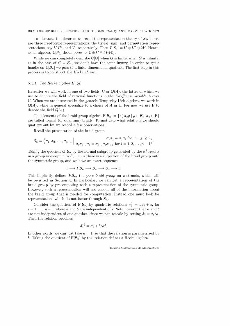
and edges labeled by a 2 become wavy lines.
0=
1=
2=
Under this new notation e0 and e1 become
.
Hereafter we will drop the dashed lines labeling the ground state. Towardsapplying Gram-Schmidt we find the inner products 〈ei, ej〉 using the graphicalcalculus.
〈e0, e0〉 = = d2 = 2
〈e1, e1〉 = =
=
2
1
1
= 1
Volumen 50, Numero 2, Ano 2016

BRAID GROUP REPRESENTATIONS AND TOPOLOGICAL QUANTUM COMPUTATION251
〈e0, e1〉 = = = 0
Exercise 4.3. Verify that 〈e1, e1〉=2 and 〈e0, e1〉 = 0 in the manner shownabove, inserting the appropriate Jones-Wenzl projectors at the trivalent verticesand using the graphical calculus.
Since 〈e0, e1〉 = 0, the choices e0 = 1√2e0 and e1 = e1 define an or-
thonormal basis {e0, e1} of V2,4,0. Then with respect to this basis, ρ(σ1) =(〈e0, σ1e0〉 〈e0, σ1e1〉〈e1, σ1e0〉 〈e1, σ1e1〉
).
For example,
〈σ1e0, e0〉 = ( 1√2)2 = 1
2 ·A + 12 ·A
−1
= 12 (A · d2 +A−1d3) = −A−3
,
where the crossings were resolved using the Kauffman bracket. Similar calcu-lations for the remaining matrix entries show that
ρ(σ1) =
(−A−3 0
0 A
).
By repeating the same method to find the remaining generators ρ(σ2) andρ(σ3), one can calculate the image ρ4,2,0(b) for any b ∈ B4.
This outlines an elementary way to find the Jones representation. Whileit has the benefit that it uses only knowledge of the Kauffman bracket andarithmetic, as n gets larger it becomes inefficient to do by hand. Additionaldata in TLJ(A) coming from its structure as a UMC provide more tools tofind ρn,k,i using graphical calculus, namely the θ-symbols, R-symbols, and F -symbols.
Revista Colombiana de Matematicas

252 COLLEEN DELANEY, ERIC C. ROWELL & ZHENGHAN WANG
4.4. θ-symbols, R-symbols, and F -symbols
Take any admissibly-labeled trivalent vertex eabc , i.e. an element of Hom(c, a⊗b).Then the θ-symbol θ(a, b, c) is defined to be the the inner product 〈eabc , eabc 〉 ofthe trivalent tree vector eabc .
θ(a, b, c) =
⟨cba
, cba
⟩
Another version of the unitary θ-symbol is related to the quantum dimensionsof the charges a, b, and c via√
dadbdc = θu(a, b, c).
Once these symbols are determined for an anyon model they can be used tohelp calculate the desired braid group representation by substituting a θ-symbolwhenever the inner product of two trivalent vertices appears.
4.4.1. R-symbols
Another set of symbols allows one to resolve crossings in the graphical calculus.Braiding gives a linear map
: Hom(c, a⊗ b)→ Hom(c, b⊗ a)
.
It is in fact an isomorphism, with inverse given by the opposite crossing. SinceHom(c, b⊗a) is one-dimensional in TLJ theory, and we already have a preferredbasis for it, namely the trivalent vertex labeled by a, b, and c, the equation
a b
c
= Rabcc
ba
holds, where Rabc is a scalar, which we call the braiding eigenvalue or R-symbol.There is a general formula that gives the R-symbols, for any Kaufmann variableA and any Temperley-Lieb category, given by
Rabc = (−1)a+b−c
2 A−[a(a+2)+b(b+2)−c(c+2)]
2 .
One can also calculate the R-symbols from their defining relation by taking theinner product of both sides of the equation with the trivalent vertex labeled by
Volumen 50, Numero 2, Ano 2016

BRAID GROUP REPRESENTATIONS AND TOPOLOGICAL QUANTUM COMPUTATION253
a, b, and c, which we demonstrate in the following example with R222 , where
the labels “2” on the right hand side of the equation indicate that every edgein the diagram is labeled by a 2.
2
2
R222 =
By resolving the top diagram via the Kauffman bracket and inserting Jones-Wenzl projectors p2 at the appropriate vertices, R22
2 can be calculated by hand.However, doing so efficiently requires familiarity with the graphical calculus andits shortcuts.
Exercise 4.4. Calculate R222 using the graphical calculus and compare with
the formula.
4.4.2. F-symbols
The other hero in the theory is the F -symbols, which tells us how to makechanges of basis in the fusion vector spaces. We consider the space Hom(d, (a⊗b)⊗ c), with orthonormal basis given by {e(ab)c
d,m }, where
e(ab)cd,m =
a b c
m
d
Similarly, we can consider the orthonormal basis {ea(bc)d,n } of Hom(d, a⊗ (b⊗c)),
where
ea(bc)d,n =
a b c
d
n
.
Revista Colombiana de Matematicas

254 COLLEEN DELANEY, ERIC C. ROWELL & ZHENGHAN WANG
Then F : {e(ab)cd,m } → {e
a(bc)d,m } is the change of basis matrix, satisfying
e(ab)cd,m =
∑F abcd,nme
a(bc)d,n .
In terms of the graphical calculus, the F -symbols allow one go back and forthbetween different ways to associate fusion vertices. The F -symbols are notori-ously hard to find, although there is a general formula. Similar to the methoddescribed in the previous section for computing the R-symbols by tracing outtheir defining relation, there is a way to calculate them using the graphicalcalculus.
For example, the two fusion trees 0/2 and 0/2 each give a basis for
the space Hom(2 ⊗ 2, 2 ⊗ 2), where each edge that is not explicitly labeled isunderstood to be labeled with a 2. Therefore they satisfy the following equa-tions.
= α + β
= γ + δ
The constants can be determined by taking the trace of each equation in twodifferent ways: once vertically and once horizontally. That is, once connectingtop and bottom edges and once connecting left and right edges. The calculationscan then be simplified using the θ-symbols. The F -matrix is then given by(α β
γ δ
).
Exercise 4.5. Use the graphical calculus to show that the F -matrix is givenby (
φ−1 φ−1/2
φ−1/2 −φ−1
).
4.5. Calculating the representation ρ3,τ⊗3,τ for the Fibonacci theory
Equipped the R and F symbols, the images of Jones representations can besystematically computed using the graphical calculus.
4.5.1. The Fibonacci R and F -symbols
When A = ±ie2πi/10, using the formula Rabc = (−1)a+b−c
2 A−[a(a+2)+b(b+2)−c(c+2)]
2
we findR22
0 = A−8 = e−4πi/5, R222 = −A−4 = −e−2πi/5.
Volumen 50, Numero 2, Ano 2016

BRAID GROUP REPRESENTATIONS AND TOPOLOGICAL QUANTUM COMPUTATION255
The Fibonacci F -matrix is given by
F =
(φ−1 φ−1/2
φ−1/2 −φ−1
).
Either of these quantities can be found using the method outlined in the pre-vious section.
4.5.2. The Jones representation ρ3,τ⊗3,τ
Given the R and F -symbols, ρ(σ1) and ρ(σ2) take the form
ρ(σ1) =
(Rττ1 0
0 Rτττ
), ρ(σ2) = Fρ(σ1)F−1
Explicitly, the generators σ1 and σ2 have representations
ρ(σ1) =
(ξ−2 0
0 −ξ−1
), ρ(σ2) =
(φ−1ξ2 −φ−1/2ξ
−φ−1/2ξ −φ−1
),
where ξ = e2πi/5 and φ is the golden ratio.
Having introduced the main tools for calculating braid group representa-tions, we turn to studying their images.
4.6. The image of the braid group representation
The basic questions that must be addressed in order to assess the utility ofthese representations for quantum computation are the following:
Question 4.6.
(1) Is the image ρk,n,i(Bn) in U(Vk,n,i) finite or infinite?
(2) If it is infinite, what is the compact Lie group ρk,n,i(Bn)?
The first question was answered by Jones in his seminal 1984 paper [11],and the second by Freedman, Larsen, and Wang in 2002 [8].
Theorem 4.6 (Jones). For k ∈ {1, 2, 4}, ρk,n,i(Bn) is a finite group. For othervalues of k and n ≥ 3, ρn,k,i(Bn) is infinite, except for when k = 8 and n = 4.
Theorem 4.7 (Freedman, Larsen, W.). When ρk,n,i(Bn) is infinite, SU(Vk,n,i) ⊂ρk,n,i(Bn).
Revista Colombiana de Matematicas

256 COLLEEN DELANEY, ERIC C. ROWELL & ZHENGHAN WANG
We will see that quantum computation is performed by applying unitarymatrices to quantum bits, so this result has important applications.
While we have stated very general results about the images of braid grouprepresentations whose proofs are beyond the scope of these notes, there aremore elementary ways that can reproduce these results in the k = 2 and k = 3case, to address whether the Ising and Fibonacci models can be useful forquantum computation.
4.6.1. The image of ρ2,4,0
The following theorem characterizes the image of the Jones representation ofthe four-strand braid group at level 2 and trivial total charge.
Theorem 4.8.
(1) For k = 2, the Temperley-Lieb-Jones algebra TLJn(A) is isomorphic toa Clifford algebra.
(2) The sequence1→ Zn2 → ρ2,n,i(Bn)→ Sn → 1
is exact projectively for n 6= 3. When n = 3, the sequence
1→ Z22 → ρ2,3,i(Bn)→ S3 → 1
is exact projectively. In particular, the projective image of the braid grouprepresentation ρ2,3,i is finite.
To prove the first part of the theorem, we’ll need to know that the Majoranaversion of a Clifford algebra is the C-span of vectors {e1, . . . , en−1}, subject tothe relation eiej + ejei = 2δij . The k = 2 Temperley-Lieb-Jones algebra interms of generators and relations is the C-span of the diagrams {u1, . . . , un−1},modulo the relation p3 = 0.
In order to show that these two algebras are isomorphic, we need a con-version between the generators ei of the Clifford algebra and the ui of theTemperley-Lieb-Jones algebra. Recall σi = A+A−1ui, and define gi = −A−1σi =−1− A−2ui. Since A is an eighth root of unity when k = 2, g2
i = 1− dui. Onthe other hand, the ei can be written as ei = (
√−1)i−1g2
i g2i−1 · · · g2
1 , so that
gi =√−1eiei+1. Then one can check that their mutual definitions with respect
to the gi agree.
The proof of the second part of the theorem can be found in [11]. We presentsome of the details here that are independent of the value of n.
Recall the pure braid group PBn, which is defined implicitly through theshort exact sequence
1→ PBn → Bn → Sn → 1,
Volumen 50, Numero 2, Ano 2016

BRAID GROUP REPRESENTATIONS AND TOPOLOGICAL QUANTUM COMPUTATION257
and can be interpreted as a group of braid diagrams whose strands begin andend in the same position. For example, the following braid on four strands is apure braid.
An important class of pure braids are those of the form σ2i for any generator σi
of Bn, since certain conjugates of σ2i form a generating set Aij of PBn, where
Aij = (σjσj−1 · · ·σi+1)σ2i (σjσj−1 · · ·σi+1)−1, i < j.
Then one can argue that the sequence
1→ ρ(PBn)→ ρ(Bn)→ ρ(Sn)→ 1
is also exact. This reduces the problem of showing that the image of the braidgroup is finite projectively (up to a scalar which is a root of unity) to theproblem of showing that the image of the pure braid group is finite projectively.
The following proposition contains the relations needed in order to showthe pure braid group image is finite projectively.
Proposition 4.9. Let gi be defined as above.
(1) g2i g
2i+1 + g2
i+1g2i = 0
(2) gig2i±1g
−1i = ig2
i g2i±1
The proof of this proposition is an exercise for the reader in the graphicalcalculus.
The first part of Proposition 4.9 tells us that the g2i ’s commute up to an
overall minus sign, and furthermore we can deduce that g16i = 1. Then it follows
from the second part of the proposition that the projective image of the purebraid group is generated by g2
i .
Thus when k = 2 the Jones representation of the braid group has finiteprojective image.
The physical consequence of 4.8 is the following result, the proof of whichrequires some familiarity with the mathematical formalism of quantum com-putation, which is discussed in the next subsection.
Corollary 4.10. The Ising theory cannot be used for universal quantum com-putation by braiding alone.
Revista Colombiana de Matematicas

258 COLLEEN DELANEY, ERIC C. ROWELL & ZHENGHAN WANG
This means that the set of quantum gates that come from the matrix repre-sentations ρ2,n,i of the braiding of the anyons {1, σ, ψ} of the Ising model is notpowerful enough to build a universal quantum computer. In order to prove thiscorollary, one needs to know about the mathematical formalism of quantumcomputation, which will be discussed shortly.
One the other hand, all of SU(2) is contained in ρ3,τ⊗3,i(B3).
4.6.2. The image of ρ3,τ⊗3,τ
The following theorem characterizes the closed images of ρ3,τ⊗3,i in U(V3,τ⊗3,i).
Theorem 4.11. ρ3,τ⊗3,i(Bn) ⊃ SU(V3,τ⊗3,i).
4.6.3. Proof of the theorem
We begin by showing that the image is infinite. Of course, it suffices to demon-strate the existence of an element in the image which is of infinite order.
Recall that the generators σ1 and σ2 have representations
ρ(σ1) =
(ξ−2 0
0 −ξ−1
)and ρ(σ2) =
(φ−1ξ2 −φ−1/2ξ
−φ−1/2ξ −φ−1
)= Fσ1F,
where φ is the golden ratio and ξ = e2πi/5. Since the matrix representation ofσ1 is diagonal, it is easy to see that its order is just the least common multipleof the orders of the roots of unity appearing on the diagonal, and hence σ1 hasorder 10. Since all elements of the braid group are in the same conjugacy class,it follows that σ2 has order 10 as well.
Consider σm1 σ2, where σ101 = 1 and m = 1, 2, . . . , 9. We claim that when
m = 4 and m = 9, both elements σm1 σ2 are of infinite order, and moreover,they don’t commute. To see that they do not commute, suppose
(σ41σ2)(σ9
1σ2) = (σ91σ2)(σ4
1σ2).
Then using that σ1 has order ten, it follows that
σ41σ2σ
−11 σ2 = σ−1
1 σ2σ41σ2
and henceσ5
1σ2 = σ2σ51 .
But one can check using the definitions of σ1 and σ2 that this is not the case.
To prove that σ41σ2 and σ9
1σ2 are of infinite order, we use established resultsabout when small sums of roots of unity vanish [4]. Suppose σ4
1σ2 is of finiteorder, then there will be two roots of unity λi, i = 1, 2 such that Tr(σ4
1σ2) =
Volumen 50, Numero 2, Ano 2016

BRAID GROUP REPRESENTATIONS AND TOPOLOGICAL QUANTUM COMPUTATION259
λ1 + λ2 and λ1λ2 = det(σ41σ2) = ξ. The trace Tr(σ4
1σ2) can be written asan integral identity of ξ and λ1. But this possibility is not among such sumsas classified in [4]. Similarly, we can show σ9
1σ2 is of infinite order. Puttingg1 = σ4
1σ2 and g2 = σ91σ2, this shows that {gm1 } = SO(2) and {gm2 } = SO(2)
both inject into SU(2), proving the theorem.
The physical corollary of this mathematical result is that {ρ(σ1), ρ(σ2)} isa universal gate set for a single qubit.
Corollary 4.12. Braiding Fibonacci anyons is enough to get any single qubitquantum gate.
But what about n-qubit gates from this representation? In general, onewould need n-qubit space (C2)⊗n to be contained in Hom(3, τ⊗n, 1). However,we will see that it is enough to get all two-qubit gates.
In the next section we provide the background necessary to assess the powerof the images of the Jones representations as quantum gates and prove the twophysical corollaries stated in this section for the Ising and Fibonacci theories.
4.7. Quantum gates and universal quantum computation
Classically, a decision problem is the following: given a sequence of functions{fn} : Zn2 to Zn2 on n-bit strings, compute fn(x) for all x ∈ Zn2 . “Quantizing”this set up, we have a quantum decision problem - given a sequence of {fn}on C[Zn2 ] ∼= (C2)⊗n, the space of n-qubits, find a unitary matrix U such thatU |x〉 = |fn(x)〉. Such matrices are written with respect to the computationalbasis Zn2 of (C2)⊗n.
We are always concerned with efficient approximation when performingcomputation. The correct notion of efficiency is that U should be a compositionof gates, of polynomial length in n, the number of qubits.
The building blocks of which such a U is composed are elements of a smallgate set, say, S = {g1, . . . , gm}, where each gi is a 2×2 or 4×4 unitary matrix,i.e. each acts on a one qubit (C2 ) or two-qubit (C2 ⊗C2) subspace of (C2)⊗n.These gate sets, while acting on a few qubits at a time, are extended triviallyon the remaining qubits by tensoring with the identity. A gate set is said tobe universal if we can build any unitary matrix to arbitrary accuracy with afinite number of elements of our gate set. More precisely, if we consider the setof all quantum circuits on (C2)⊗n that can be built from our gate set, then itis universal if it is dense in SU(2n). (Recall that we are interested in thingsup to a phase.) The rest of this section is devoted to demonstrating that singleand double-qubit operators are enough to get universal quantum computation.
Revista Colombiana de Matematicas
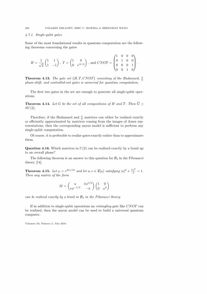
260 COLLEEN DELANEY, ERIC C. ROWELL & ZHENGHAN WANG
4.7.1. Single-qubit gates
Some of the most foundational results in quantum computation are the follow-ing theorems concerning the gates
H =1√2
(1 1
1 −1
), T =
(1 0
0 eiπ/4
), and CNOT =
1 0 0 0
0 1 0 0
0 0 0 1
0 0 1 0
.
Theorem 4.13. The gate set {H,T,CNOT} consisting of the Hadamard, π8
phase-shift, and controlled-not gates is universal for quantum computation.
The first two gates in the set are enough to generate all single-qubit oper-ations.
Theorem 4.14. Let G be the set of all compositions of H and T . Then G ⊃SU(2).
Therefore, if the Hadamard and π8 matrices can either be realized exactly
or efficiently approximated by matrices coming from the images of Jones rep-resentations, then the corresponding anyon model is sufficient to perform anysingle-qubit computation.
Of course, it is preferable to realize gates exactly rather than to approximatethem.
Question 4.16. Which matrices in U(2) can be realized exactly by a braid upto an overall phase?
The following theorem is an answer to this question for B3 in the Fibonaccitheory [14].
Theorem 4.15. Let ω = e2πi/10 and let u, v ∈ Z[ω] satisfying |u|2 + |v|2φ = 1.
Then any matrix of the form
M =
(u vφ1/2
vφ−1/2 −u
)(1 0
0 ωk
)can be realized exactly by a braid in B3 in the Fibonacci theory.
If in addition to single-qubit operations an entangling gate like CNOT canbe realized, then the anyon model can be used to build a universal quantumcomputer.
Volumen 50, Numero 2, Ano 2016

BRAID GROUP REPRESENTATIONS AND TOPOLOGICAL QUANTUM COMPUTATION261
4.7.2. Two-qubit gates and entanglement
The notion of entanglement is key to understanding universality.
Definition 4.16. A gate g in U(4) is not entangling if either g = A ⊗ B or
SWAP g = A⊗B, where A,B ∈ U(2) and SWAP =
1 0 0 0
0 0 1 0
0 1 0 0
0 0 0 1
. If a gate
is not of this form, then it is called entangling.
The simplest example of an entangling gate is the CNOT gate. To show thatCNOT is entangling, we must prove that neither CNOT nor SWAP CNOT canbe written as a tensor product A ⊗ B, for any A,B ∈ U(2). Recall that theCNOT has the following matrix with respect to the computational basis.
CNOT =
1 0 0 0
0 1 0 0
0 0 0 1
0 0 1 0
If a matrix M can be written M = M1⊗M2, where M1 has eigenvalues λi andM2 has eigenvalues µj , then the eigenvalues of M are of the form λiµj . CNOThas eigenvalues 1, 1, 1,−1. So if there were matrices A and B with eigenvaluesλ1, λ2 and µ1, µ2 respectively, then they would have to satisfy the system ofequations
λ1µ1 = 1
λ1µ2 = 1
λ2µ1 = 1
λ2µ2 = −1
.
But detλij = 0, so this cannot happen. The same argument applies to showthat SWAP CNOT cannot be written as a tensor product. Therefore the CNOTgate is entangling.
Any four-by-four unitary matrix, that is, any two-qubit quantum gate, canbe written as a tensor product of single-qubit gates and an entangling gate, asthe following theorem states.
Theorem 4.17. Given any entangling gate E, any matrix in U(4) can bewritten as a finite product of some number of E’s and matrices in U(2) up toan overall phase.
This takes care of two-qubit gates. To be able to construct n-qubit gatesfrom one and two-qubit gates we need the following definition.
Revista Colombiana de Matematicas

262 COLLEEN DELANEY, ERIC C. ROWELL & ZHENGHAN WANG
Definition 4.18. A matrix is 2-level if it is not the identity only on a 2-dimensional subspace.
An important example of a 2-level matrix for our purposes is of the kind 1 0
0 10
0 U
,
where U ∈ U(2).
The following lemma collects the facts that allow local unitary computation.
Lemma 4.19. Every unitary matrix M is a product of 2-level unitary matrices.Every 2-level matrix can be realized as a product of 1-qubit gates and CNOTs.
The results we have collected thus far imply the following theorem.
Theorem 4.20. The CNOT gate, together with SU(2) forms a universal gateset. That is, if U ∈ SU(2n), then U can be written as a tensor product ofCNOT gates and 2× 2 unitary matrices.
All of the linear algebra is now in place to understand what is needed for asmall gate set to be universal.
4.8. Ising and Fibonacci quantum computers
Since the image of ρ2,4,0 is finite in U(2), we can’t get a universal gate set fromthe Ising theory. On the other hand, we have shown that the closure of theimage of ρ3,τ⊗3,τ contains SU(2), and hence can produce any single-qubit gate.Moreover, the image of ρ3,τ⊗6,1 : B6 → U(5) can be used to approximate anentangling gate, as implied by the theorem below.
In the dense encoding, we choose the two-qubit computation subspace inV3,τ⊗6,1 as indicated by the fusion tree below.
1
τ τ τ ττ τ
ix
jτ
V3,τ⊗6,1 is 5-dimensional. When x = 1, there is only one admissible labeling,so it spans a one-dimensional subspace of V3,τ⊗6,1. We will not use this sub-space for computation, so it will be called a non-computational subspace. When
Volumen 50, Numero 2, Ano 2016

BRAID GROUP REPRESENTATIONS AND TOPOLOGICAL QUANTUM COMPUTATION263
x = τ , then all choices of i, j ∈ {1, τ} are admissible, so we obtain a naturaltwo-qubit subspace of V3,τ⊗6,1. We will denote the 4 basis elements as {eij}.Ideally, we would like to find an entangling braid b ∈ B6 on V3,τ⊗6,1 so that theresulting matrix ρ(b) is the identity on the non-computational subspace and anentangling gate on the two-qubit subspace. But we do not know the existenceof such braiding gates. It would be extremely interesting to know if such “noleakage” entangling braiding gates exist or not. But in practice, we will usethe following density theorem to find entangling braiding gates with arbitrarilysmall leakage to the non-computational subspace.
Theorem 4.21.
(1) SU(5) ⊂ ρ3,τ⊗6,1(B6).
(2) Any matrix in SU(4) can be approximated to any precision by the gate set{ρ(σi), i = 1, ..., 5} on the computational subspace C[{eij}], i, j ∈ {1, τ}.
The proof of this theorem is not elementary so we omit the details. Pre-sumably we can use an inductive argument using irreducibility and density ofone-qubit gates Thm. 4.11. Therefore a universal gate set can be built frombraiding Fibonacci anyons, proving Theorem 1.1 for r = 5.
Open problem 4.24. Is there a two-qubit entangling gate that can be realizedby braiding exactly in the Fibonacci theory?
4.9. General TLJ theory for quantum computing
In earlier sections, we explain Ising and Fibonacci theories. In general any TLJtheory can be used for anyonic quantum computation.
The Jones-Kauffman theory at level k = r − 2 ≥ 1 is the TQFT associatedto the TLJ theory with the choice of
A =
ie−2πi/4r k ≡ 0 mod 2
ie2πi/4 k ≡ 1 mod 2 and k ≡ 1 mod 4
−ie−2πi/4 k ≡ 1 mod 2 and k ≡ −1 mod 4.
When k is even, the TLJ category is a unitary modular category modelinganyons, while when k is odd, it is a unitary pre-modular category modelingfermions. This generalizes the Ising and Fibonacci theories.
5. Approximation of The Jones polynomial
Recall that unlike the Alexander polynomial, for which their exists a polyno-mial time algorithm, computing the Jones polynomial is hard. The classicalcomplexity of computing the Jones polynomial exactly at roots of unity issummarized in the following theorem [22, 9].
Revista Colombiana de Matematicas

264 COLLEEN DELANEY, ERIC C. ROWELL & ZHENGHAN WANG
Theorem. For r 6= 1, 2, 3, 4, 6, computing the Jones evaluations J(L, e2πi/r)exactly is #P hard. Moreover, the Jones evaluations {J(L, e2πi/r)} for all linksL at r 6= 1, 2, 3, 4, 6 is dense in C.
However, the Jones evaluations at roots of unity could be efficiently approx-imated by a quantum computer. In this section we discuss an algorithm for suchan approximation which is a consequence of the efficient simulation of TQFTswith several clarifications [7]. Our approximation goes through the Jones rep-resentations of the braid group, necessitating a choice of a braid closure to turnbraids into links. For our algorithm, we use the plat closure of braids with aneven number of strands. It was observed that if instead the braid closure isused, the approximation is potentially easier [13]. Approximations have vari-ations [15], and our approximation is an additive one. Strictly speaking, weapproximate the normalized Jones evaluations: J(L, e±2πi/r) divided by dn.For the plat closures of braids b ∈ B2n, the unlink of n-components has thelargest absolute value dn. It is known that the distributions of Jones evalua-tions J(L, e±2πi/r) for r 6= 1, 2, 3, 4, 6 are limiting to a Gaussian as n→∞ [9].Hence, a Jones evaluation is typically small. Our BQP-complete theorem foran additive approximation with an error scaling as the inverse of a polynomialin n the number of strands and m the braid length, implies that the normalizedJones evaluation cannot be always exponentially small because otherwise, wecould just set the approximation to be 0.
Recall that the Jones evaluation J(L, e±2πi/r) is a map from the set oforiented links to Z[q±1/2] for q = e±2πi/r. In order to turn the evaluation atroots of unity into a computation problem, we must encode a link L and theJones evaluation J(L, e±2πi/r) as bit strings, whereupon it becomes a Boolean
map Zn2 → Zm(n)2 , that sends the bit strings encoding of the input L to the bit
strings encoding of the output J(L; e±2πi/r).
How does one turn a link into a bit string? First one presents L as the
plat-closure of some braid, say L = σskik · · ·σs1i1
. Then the integers {ij} and {sj}can be written in terms of their binary expansions and finally converted intobit strings.
As for encoding J(L, e±2πi/r) as a bit string, one can use the binary expan-sions of its real and imaginary parts. In general these binary expansions will beinfinitely long. In our algorithm we are going to approximate the evaluations.Therefore, once we are given the error ε, we can decide where to truncate theinfinite bit strings.
The following table organizes the known complexity results concerning thecomputation and approximation of the Jones polynomial at roots of unity oforder r 6= 1, 2, 3, 4, 6 [22, 15, 7, 8].
Volumen 50, Numero 2, Ano 2016

BRAID GROUP REPRESENTATIONS AND TOPOLOGICAL QUANTUM COMPUTATION265
Exactly Approximately
Classically #P No FPRAS
Quantum mechanically ? BQP-complete
5.1. Approximating Jones evaluations by a quantum computer
How is the Jones polynomial of a link L evaluated by an anyonic quantumcomputer at a root of unity? Suppose b ∈ B2n is a braid whose closure givesthe link L. Physically, a “cup” state is prepared by creating n pairs of anyonsfrom the vacuum. Then the anyons are braided by b. Then measurement isperformed by projecting onto a “cap state”. This computes |〈 cap |ρ(b)| cup 〉|2,which recovers the normalized Jones evaluations. The figure below illustratesthe process, which corresponds to the mathematical operation of taking theplat closure of b.
〈 cap |ρ(b)| cup 〉 = b
· · ·
· · ·
Classically, this computation is hard, as one might expect given the exponentialsize of ρ(b). However, there exists an efficient quantum algorithm to approxi-mate the evaluations of the Jones polynomial [7], cf. Theorem 1.2. Precisely,we have:
Theorem 5.1. Let q = e±2πi/r, d = 2 cosπ/r,σP the plat closure of σ ∈ B2n,and J(σP , q) :
⊔∞n=1 B2n → Z[q±1/2] the Jones evaluation. Given m = |σ|, n,
there exists a quantum circuit of size polynomial in n, m and 1/ε = poly(n,m)such that UL outputs a random variable Z(σ), where 0 ≤ Z(σ) ≤ 1, and∣∣∣∣∣ |J(σP , q)|2
dn− Z(σ)
∣∣∣∣∣ < ε.
Such an approximation is called an “additive” scheme. The full details of theproof are not provided here and can be found in [23, 1]. We will simply illustratethe main steps and ideas.
5.2. Encoding basis vectors as bit strings
For an illustration of this step, that of converting basis vectors into bit strings,we consider the case k = 3 and the six-strand braid group B6. Given the fusion
Revista Colombiana de Matematicas

266 COLLEEN DELANEY, ERIC C. ROWELL & ZHENGHAN WANG
tree in Hom(0, 1⊗6), we attach a qubit at each vertex with basis |i1i2i3i4〉,
0
1 1 1 11 1
a1a2
a3
1
where ij ∈ {0, 1} and aj ∈ {0, 2}. If aj = 0, we take ij = 0, and if aj = 2, thenwe take ij = 1. Then we can define the map a1a2a3 7→ |i1i2i3i4〉. This gives anefficient embedding of a basis of V3,6,0 into bit strings.
5.3. Simulating the Jones representation
When we use anyons for quantum computation, we choose a computationalsubspace (C2)⊗l in Vk,1⊗m,0. Now for the simulation of the Jones representa-tion Vk,m,0, we seek a quantum circuit U which makes the following diagramcommute. By turning basis into bit strings, Vk,m,0 is embedded as a subspacein (C2)⊗(m−2). The Jones representation of Bm is extended to (C2)⊗(m−2) bythe identity on the orthonormal complement of embedded Vk,m,0.
(C2)⊗l �� // Vk,1⊗m,0
� � //
ρ(σ)
��
(C2)⊗(m−2)
U
��Vk,1⊗m,0
� � // (C2)⊗(m−2)
We must compute the braid group action on the basis of Vk,m,0. By thinkingabout how the braid group generators act on Vk,m,0, we are led to pieces offusion trees like the ones below, those diagrams now being drawn horizontally.
x yz
i i+ 1
F -move
x
i i+ 1
y
z′
The diagram on the left can be changed to the form on the right via an F -move,and then the braiding can be removed using an R-symbol. In this manner,by stacking the braid group generators on a basis element of Vk,1⊗m,0 andthen using the graphical calculus to resolve it into a linear combination of ourcomputational basis elements, the Jones representation can be calculated for
Volumen 50, Numero 2, Ano 2016

BRAID GROUP REPRESENTATIONS AND TOPOLOGICAL QUANTUM COMPUTATION267
any n. The important observation is that the extended Jones representation isnow local: the 2-level matrix in the definition of the Jones representation actsnow on only two qubits. In physical terms, since everything is localized, weonly need to concern ourselves with two qubits at a time.
Finally, due to the fusion rules for basis elements of Vk,1⊗m,0, the Jonesrepresentation is a composition of a sequence of multi-qubit controlled 2-qubitgates on (C2)⊗(m−2). Such controlled gates can be implemented efficiently on aquantum computer using a few ancillary qubits. Therefore, we can approximatethe Jones evaluations efficiently by a quantum computer.
6. Localization of braid group representations
The quantum circuit model is explicitly local: the n-qubit spaces are tensorpowers (C2)⊗n and the n-qubit circuits are composed of gates (e.g. promotionsof SWAP, CNOT) that act nontrivially on just a few adjacent qubit spaces.
In contrast, the topological model relies upon gates that are not explicitlylocal, coming from representations of the braid group. So far we have metseveral families of Bn representations: the local representations ρR associatedwith an R-matrix, the Burau representations ρ and their reduced versions ρand the Jones representations (generic and specialized). In subsection 4.6.2we gave a detailed version of Theorem 1.1, which is the main result of [8].Consequently, the quantum circuit model (hence a quantum Turing machine)can be efficiently simulated on a topological quantum computer via certainlevel k Jones representations of the braid group.
The main theorem (i.e. Theorem 1.2) of [7] is a partial converse: the spe-cialized Jones polynomial can be efficiently approximated on the quantumcircuit model (cf. Section 5). This is achieved by exploiting a hidden localityin topological quantum field theory, which we now outline. Recall from Sub-section 4.1.3 that the labels for the Temperley-Lieb-Jones category at levelk are L := {0, . . . , k}. The Bn representation obtained from the standardfaithful TLn(A)-module is H :=
⊕j Hom(j, 1⊗n). Here each direct summand
Hj = Hom(j, 1⊗n) is an irreducible Bn representation associated with a diskwith n interior points marked with the anyon type 1 and the boundary labelledj. Now we decompose our n-punctured disks into n−1 pairs of pants by makingn−2 concentric circular cuts for each boundary label j. The gluing and disjointunion axioms then show that
H =⊕
(i1,...,in−1)∈Ln−1
Hom(1⊗2, i1)⊗Hom(1⊗ i1, i2)⊗· · ·⊗Hom(1⊗ in−2, in−1).
Here the boundary label is j = in−1. Now we set V =⊕
(a,b,c) Hom(a ⊗ b, c)and distribute ⊗ over ⊕ to realize H inside V ⊗(n−1). The complement H⊥ of Hinside V ⊗(n−1) does not typically admit a braid group action. Alternatively wecan be slightly more efficient and take U =
⊕(b,c) Hom(1⊗ b, c). The upshot is
Revista Colombiana de Matematicas

268 COLLEEN DELANEY, ERIC C. ROWELL & ZHENGHAN WANG
that the specialized Jones representations of Bn can be realized inside a vectorspace of the form V ⊗f(n), but with Bn only acting on a certain hidden subspace.One may employ the same technique for the Fibonacci representations.
Exercise 6.1. Set k = 2 and show that dim(V ) = 10, while dim(U) = 4.Observe that for the B3 representation we have dim(V3,1) = 2, where V3,1 isembedded into either V ⊗2 or U⊗2, and so has a very large complement.
This gross inefficiency motivates the following:
Question 6.2. When can a family of Bn representations be realized locally(uniformly for all n, and “on the nose”)?
Eventually we will restrict to unitary representations, but first we mustmake sense of what sort of families we are interested in.
6.1. Sequences of Bn Representations
Notice that we have natural injective group homomorphisms ι : Bn → Bn+1
given by ι(σi) = σi, for 1 ≤ i ≤ n− 1 allowing us to identify Bn as a subgroupof Bn+1
3. Which families of representations respect these identifications? Forprecision’s sake we phrase the following in terms of group algebras [20]:
Definition 6.2. An indexed family of complex Bn-representations (ρn, Vn)is a sequence of braid representations if there exist injective algebra homo-morphisms ϕn : Cρn(Bn) → Cρn+1(Bn+1) such that the following diagramcommutes:
CBnρn //
� _
ι
��
Cρn(Bn)� _
ϕn
��CBn+1
ρn+1// Cρn+1(Bn+1)
Example. If R is a solution to the Yang-Baxter equation on a vector space V ,then it is easy to see that ρn : CBn → End(V ⊗n) given by ρn(σi) = I⊗i−1
V ⊗R ⊗ I⊗n−i−1
V is a sequence of braid representations: take ϕn : End(V ⊗n) →End(V ⊗n+1) to be ϕn(f) = f ⊗ IV .
The Jones representations (specialized or not) and the (related) Fibonaccirepresentations ρn,τ are sequences in this sense. For example, for the genericJones representation we have Cρn(Bn) = TLn(A) and Cρn+1(Bn+1) = TLn+1(A).Letting ϕn(ui) = ui we see that the appropriate diagram commutes.
Example. The Burau (reduced or unreduced) representations do not form asequence of Bn representations in our sense. Indeed in the case where ρ is
3Of course there are many less natural injective homomorphisms, for example σi 7→(σn−i+1)−1 can be verified as an injective homomorphism.
Volumen 50, Numero 2, Ano 2016

BRAID GROUP REPRESENTATIONS AND TOPOLOGICAL QUANTUM COMPUTATION269
irreducible, we have Cρ(Bn) ∼= Mn−1(C) (for all n). Since there are no injectivehomomorphisms from Mn−1(C) to Mn(C), the required map ϕn does not exist.
Exercise 6.3. Show that the standard permutation representations of Sn,lifted to Bn in the obvious way via (i i+1) 7→ σi is not a sequence in our sense.
Now we can describe what we mean by a localization of a sequence of braidgroup representations.
Definition 6.4. Suppose (ρn, Vn) is a sequence of braid representations. Alocalization of (ρn, Vn) is a braided vector space (W,R) with R ∈ U(W⊗2) suchthat for all n ≥ 2 there exist injective algebra homomorphisms ψn : Cρ(Bn)→End(W⊗n) satisfying ψn ◦ ρ(b) = ρR(b) for b ∈ Bn.
This definition may seem a bit complicated at first, but encapsulates thenotion of “on the nose” local realizations of a sequence of Bn representations.From the point of view of quantum computation, we are trying to discoverwhen the singleton gate set {R} can simulate all braiding gates. In spite of theslightly mystifying definition, the idea is quite simple: we want to find a singlesolution to the Yang-Baxter equation R on a vector space W so that
(1) For each n, (ρn, Vn) is a sub-representation of (ρR,W⊗n). Notice that we
distinguish between equivalent irreducible sub-representations of Vn: if `isomorphic copies of some fixed irreducible U appears in Vn then W⊗n
must contain at least ` copies of U . This is a distinction at the levelof algebras: C2 is not a faithful representation of M2(C) ⊕M2(C), butC2 ⊕ C2 is.
(2) There are no irreducible Bn-subrepresentations of W⊗n that do not ap-pear in Vn. Whereas the hidden locality of [7] has a large non-computationalspace upon which the braid group does not act, we are asking that thereis no such axillary space.
Comparing with the property F conjecture, we obtain:
Conjeture 6.6. Suppose (V,R) is a unitary solution to the YBE such that Rhas finite (projective) order, with corresponding Bn-representations (ρR, V
⊗n).Then ρR(Bn) is a finite group (projectively).
If the words unitary or finite order are omitted Conjecture 6.1(a) is false,see [20] for examples.
6.2. Non-localizable representations
In the braided fusion category setting Conjecture 6.1 is closely related to an-other fairly recent conjecture (see [19, Conjecture 6.6]). Braided fusion cate-gories are naturally divided into two classes according to the algebraic com-plexity of their fusion rules. In detail, one defines the Frobenius-Perron di-mension FPdim(X) of an object X in a fusion category C to be the largest
Revista Colombiana de Matematicas
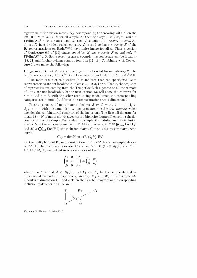
270 COLLEEN DELANEY, ERIC C. ROWELL & ZHENGHAN WANG
eigenvalue of the fusion matrix NX corresponding to tensoring with X on theleft. If FPdim(Xi) ∈ N for all simple Xi then one says C is integral while ifFPdim(Xi)
2 ∈ N for all simple Xi then C is said to be weakly integral. Anobject X in a braided fusion category C is said to have property F if theBn-representations on End(X⊗n) have finite image for all n. Then a versionof Conjecture 6.6 of [19] states: an object X has property F if, and only if,FPdim(X)2 ∈ N. Some recent progress towards this conjecture can be found in[18, 21] and further evidence can be found in [17, 16]. Combining with Conjec-ture 6.1 we make the following:
Conjeture 6.7. Let X be a simple object in a braided fusion category C. Therepresentations (ρX ,End(X⊗n)) are localizable if, and only if, FPdim(X)2 ∈ N.
The main result of this section is to indicate that the specialized Jonesrepresentations are not localizable unless r = 1, 2, 3, 4 or 6. That is, the sequenceof representations coming from the Temperley-Lieb algebras at all other rootsof unity are not localizable. In the next section we will show the converse forr = 4 and r = 6, with the other cases being trivial since the correspondingcategories are pointed (and hence the representations are 1-dimensional).
To any sequence of multi-matrix algebras S := C = A1 ⊂ · · · ⊂ Aj ⊂Aj+1 ⊂ · · · with the same identity one associates the Bratteli diagram whichencodes the combinatorial structure of the inclusions. The Bratteli diagram fora pair M ⊂ N of multi-matrix algebras is a bipartite digraph Γ encoding the de-composition of the simple N -modules into simple M -modules, and the inclusionmatrix G is the adjacency matrix of Γ. More precisely, if N ∼=
⊕tj=1 End(Vj)
and M ∼=⊕s
i=1 End(Wi) the inclusion matrix G is an s× t integer matrix withentries:
Gi,j = dim HomM (ResNM Vj ,Wi)
i.e. the multiplicity of Wi in the restriction of Vj to M . For an example, denoteby Mn(C) the n × n matrices over C and let N = M4(C) ⊕M2(C) and M ∼=C⊕ C⊕M2(C) embedded in N as matrices of the form:a 0 0
0 a 0
0 0 A
⊕ (a 0
0 b
)
where a, b ∈ C and A ∈ M2(C). Let V1 and V2 be the simple 4- and 2-dimensional N -modules respectively, and W1, W2 and W3 be the simple M -modules of dimension 1, 1 and 2. Then the Bratteli diagram and correspondinginclusion matrix for M ⊂ N are:
W1
�� !!
W2
��
W3
vvV1 V2
Volumen 50, Numero 2, Ano 2016

BRAID GROUP REPRESENTATIONS AND TOPOLOGICAL QUANTUM COMPUTATION271
and 2 1
0 1
1 0
.
The Bratteli diagram for the sequence S is the concatenation of the Brattelidiagrams for each pair (Ak, Ak+1), with corresponding inclusion matrix Gk. Weorganize this graph into levels (or stories) corresponding to each algebra Ak sothat the Bratteli diagram (Ak−1, Ak) is placed above the vertices labelled bysimple Ak-modules, and that of (Ak, Ak+1) is placed below. Having fixed anorder on the simple Ak-modules we record the corresponding dimensions in avector dk. Observe that dk+1 = GTk dk.
Let us illustrate this for the Fibonacci theory corresponding to the coloredTLJ-theory at A = ie2πi/20. Here we have two labels 1 and τ as in subsection4.2.3. Decomposing the simple TLJn(A) modules for this theory as TLJn−1(A)modules for n = 1, 2, . . . we have:
τ
�� ��1
��
τ
�� ��τ
�� ��
1
��1 τ
For each n > 1, TLJn(A) has two simple modules: V1,n := Hom(1, τ⊗n) andVτ,n := Hom(τ, τ⊗n). Moreover, Cρn(Bn) = TLJn(A) so these are irreducibleBn-representations. Let us compute the inclusion matrices as above, orderingthe modules [V1,n, Vτ,n] in spite of the alternating arrangement of the Brattelidiagram. Since V1,n|Bn−1
∼= Vτ,n−1 and Vτ,n|Bn−1∼= V1,n−1⊕Vτ,n−1 we have: are
G = Gn =
(0 1
1 1
)for all n > 1. By computing powers of G one can see that
dim(V1,n) = fn−1 and dim(Vτ,n) = fn where f0 = 1, f1 = 1, f2 = 1, f3 = 2, . . .is the Fibonacci sequence.
Now suppose that we could find a Yang-Baxter matrix R on a space Wof dimension d localizing the sequence of Bn-representations (ρn, V1,n ⊕ Vτ,n).Using the algebra injections ψn, the space W⊗n becomes a TLJn(A)-moduleand hence W⊗n ∼= anV1,n ⊕ bnVτ,n as TLJn(A) (or Bn) modules with an ≥ 1,bn ≥ 1 multiplicities. Notice that dn = anfn−1 + bnfn for all n > 1. Wecan use G to inductively express the multiplicities (an, bn). Indeed, since re-stricting anV1,n ⊕ bnVτ,n to Bn−1 we get bnV1,n−1 ⊕ (an + bn)Vτ,n−1, we have
Revista Colombiana de Matematicas

272 COLLEEN DELANEY, ERIC C. ROWELL & ZHENGHAN WANG
G(an, bn)T = (an−1, bn−1). Notice also that G(fn−2, fn−1)T = (fn−1, fn). Thusthe formula dn = anfn−1 + bnfn valid for all n > 1 gives us the two equations:〈(an, bn), G(fn−2, fn−1)〉 = dn and 〈G(an, bn), (fn−1, fn)〉 = dn−1. But sinceGT = G we have
dn = 〈(an, bn), G(fn−2, fn−1) rangle = 〈G(an, bn), (fn−1, fn)〉 = dn−1,
a contradiction. So the Fibonacci theory cannot be localized.
This may seem a bit ad hoc, but in fact this can be generalized wheneverthe Bratteli diagram for Cρn(Bn) ⊂ Cρn+1(Bn+1) is periodic of some periodk. In this case there is a strictly positive integer-valued square matrix G thatdescribes the inclusion of Cρn(Bn) ⊂ Cρn+k(Bn+k). One then applies the thePerron-Frobenius theorem to see that some vector of multiplicities bn is aneigenvector of G corresponding to the largest eigenvalue λ of G. This impliesthat λ ∈ Z, since G and bn are integral, which often leads to a contradiction(see [20] for details).
6.3. Jones representation at levels 2 and 4
In this section we give explicit localizations for the Jones representations atlevels 2 and 4.
For the Ising theory (level 2) an explicit localization appears in [6]. Theobjects are 1, σ and ψ where FPdim(σ) =
√2 and FPdim(ψ) = 1. The Bratteli
diagram is:σ
�� ��1
��
ψ
��σ
and the matrix
−e−πi/4√2
1 0 0 1
0 1 −1 0
0 1 1 0
−1 0 0 1
gives an explicit localization (see [6, Section 5]).
At level 4 (A = ie−2πi/24), the categorical model is a rank 5 category withsimple objects 1, Z of dimension 1, Y of dimension 2 and X,X ′ of dimension√
3. The fusion rules for this category are determined by:
X ⊗X ∼= 1⊕ Y, X ⊗X ′ ∼= Z ⊕ Y(1)
X ⊗ Y ∼= X ⊕X ′, Z ⊗X ∼= X ′.(2)
Volumen 50, Numero 2, Ano 2016

BRAID GROUP REPRESENTATIONS AND TOPOLOGICAL QUANTUM COMPUTATION273
The Bratteli diagram (starting at level 1) is shown in below.
X
�� 1
��
Y
~~ ��X
��
X ′
�� 1
��
Y
~~ ��
Z
~~X
��
X ′
�� 1 Y Z
We have TLJn(A) ∼= End(X⊗n) for each n, where the isomorphism is inducedby
gi ↔ Id⊗i−1X ⊗ cX,X ⊗ Id⊗n−i−1
X ∈ End(X⊗n).
Here cX,X is the (categorical) braiding on the object X. The irreducible sec-tors of TLJn(A) under this isomorphism are the End(X⊗n)-modules Hn,W :=Hom(W,X⊗n) where W is one of the 5 simple objects in C. Observe that for neven W must be one of 1, Y or Z while for n odd W is either X or X ′. We havethe following formulae for the dimensions of these irreducible representations(for n odd):
dim Hom(X,X⊗n) =3
n−12 + 1
2, dim Hom(X ′, X⊗n) =
3n−12 − 1
2,
dim Hom(1, X⊗n+1) =3
n−12 + 1
2, dim Hom(Y,X⊗n+1) = 3
n−12 ,
dim Hom(Z,X⊗n+1) =3
n−12 − 1
2
We present the explicit localization, referring the reader to [20] for a completeproof. Here ω = e2πi/3 is a 3rd root of unity.
Revista Colombiana de Matematicas
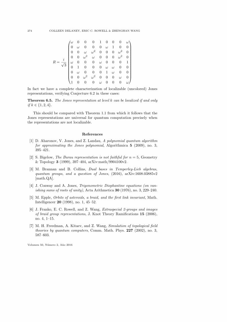
274 COLLEEN DELANEY, ERIC C. ROWELL & ZHENGHAN WANG
R =i√3
ω 0 0 0 1 0 0 0 ω
0 ω 0 0 0 ω 1 0 0
0 0 ω ω2 0 0 0 ω2 0
0 0 ω2 ω 0 0 0 ω2 0
ω 0 0 0 ω 0 0 0 1
0 1 0 0 0 ω ω 0 0
0 ω 0 0 0 1 ω 0 0
0 0 ω2 ω2 0 0 0 ω 0
1 0 0 0 ω 0 0 0 ω
In fact we have a complete characterization of localizable (uncolored) Jonesrepresentations, verifying Conjecture 6.2 in these cases:
Theorem 6.5. The Jones representation at level k can be localized if and onlyif k ∈ {1, 2, 4}.
This should be compared with Theorem 1.1 from which it follows that theJones representations are universal for quantum computation precisely whenthe representations are not localizable.
References
[1] D. Aharonov, V. Jones, and Z. Landau, A polynomial quantum algorithmfor approximating the Jones polynomial, Algorithmica 5 (2009), no. 3,395–421.
[2] S. Bigelow, The Burau representation is not faithful for n = 5, Geometry& Topology 3 (1999), 397–404, arXiv:math/9904100v2.
[3] M. Brannan and B. Collins, Dual bases in Temperley-Lieb algebras,quantum groups, and a question of Jones, (2016), arXiv:1608.03885v2[math.QA].
[4] J. Conway and A. Jones, Trigonometric Diophantine equations (on van-ishing sums of roots of unity), Acta Arithmetica 30 (1976), no. 3, 229–240.
[5] M. Epple, Orbits of asteroids, a braid, and the first link invariant, Math.Intelligencer 20 (1998), no. 1, 45–52.
[6] J. Franko, E. C. Rowell, and Z. Wang, Extraspecial 2-groups and imagesof braid group representations, J. Knot Theory Ramifications 15 (2006),no. 4, 1–15.
[7] M. H. Freedman, A. Kitaev, and Z. Wang, Simulation of topological fieldtheories by quantum computers, Comm. Math. Phys. 227 (2002), no. 3,587–603.
Volumen 50, Numero 2, Ano 2016

BRAID GROUP REPRESENTATIONS AND TOPOLOGICAL QUANTUM COMPUTATION275
[8] M. H. Freedman, M. J. Larsen, and Z. Wang, A modular functor whichis universal for quantum computation, Comm. Math. Phys. 227 (2002),no. 3, 605–622.
[9] M.H. Freedman, M. J. Larsen, and Z. Wang, The two-eigenvalue problemand density of Jones representation of braid group, Comm. Math. Phys.228 (2002), no. 1, 177–199.
[10] W. Fulton and J.Harris, Representation theory, a first course, Springer,New York, 1991.
[11] V.F.R. Jones, Braid groups, Hecke algebras and type II1 factors, Geomet-ric methods in operator algebras 123 (1983), 242–273.
[12] , Hecke-algebra representations of braid groups and link polynomi-als, Ann. Math. 126 (1987), 335–288.
[13] S.P. Jordan and P.W. Shor, Estimating Jones polynomials is a completeproblem for one clean qubit, Quantum Information and Computation 8(2008), no. 8, 681–714.
[14] V. Kliuchnikov, A. Bocharov, and K. M. Svore., Asymptotically opti-mal topological quantum compiling, Physical Review Letters 112 (2014),no. 140504, 335–288.
[15] G. Kuperberg, How hard is it to approximate the Jones polynomial?,(2009), arXiv:0908.0512v2 [quant-ph].
[16] M.J. Larsen and E.C. Rowell, An algebra-level version of a link-polynomialidentity of Lickorish, Math. Proc. Cambridge Philos. Soc. 144 (2008),no. 3, 623–638.
[17] M.J. Larsen, E.C. Rowell, and Z. Wang, The N -eigenvalue problem andtwo applications, Int. Math. Res. Not. 2005 (2005), no. 64, 3987–4018.
[18] D. Naidu and E.C. Rowell, A finiteness property for braided fusion cate-gories, Algebr. Represent. Theory 15 (2011), no. 5, 837–855.
[19] E. C. Rowell, R. Stong, and Z. Wang, On classification of modular tensorcategories, Comm. Math. Phys. 292 (2009), no. 2, 343–389.
[20] E. C. Rowell and Z. Wang, Localization of unitary braid representa-tions, Comm. Math. Phys. 311 (2012), no. 3, 595–615, arXiv:1009.0241v2[math.RT].
[21] E.C. Rowell, Braid representations from quantum groups of exceptional Lietype, Rev. Un. Mat. Argentina 51 (2010), no. 1, 165–175.
Revista Colombiana de Matematicas

276 COLLEEN DELANEY, ERIC C. ROWELL & ZHENGHAN WANG
[22] D.L. Vertigan, On the computational complexity of Tutte, Jones, Homflyand Kauffman invariants, Dissertation, University Of Oxford, 1991.
[23] Z. Wang, Topological quantum computation, Amer-ican Mathematical Society, Providence (2008),http://www.math.ucsb.edu/zhenghwa/data/course/cbms.pdf.
(Recibido en julio de 2016. Aceptado en noviembre de 2016)
Department of Mathematics
University of California Santa Barbara
Santa Barbara, CA, U.S.A.
e-mail: [email protected]
Department of Mathematics
Texas A&M University
College Station, TX, U.S.A
e-mail: [email protected]
Department of Mathematics, Microsoft Station Q
University of California Santa Barbara
Santa Barbara, CA, U.S.A.
e-mail: [email protected]
Volumen 50, Numero 2, Ano 2016


![Singular Unitary Representations and Indefinite Harmonic ...jawolf/publications.pdf/paper_092.pdfdiscrete series representations in terms of L,-cohomology groups [31,32]. We suppose](https://img.dokumen.tips/doc/110x75/5fbf13b8d2f5fd5acd562f37/singular-unitary-representations-and-indefinite-harmonic-jawolfpublicationspdfpaper092pdf.jpg)
![Tempered automorphic representations of the unitary grouppreprints.ihes.fr/2011/M/M-11-17.pdf · Rogawski [Rog90] studied irreducible admissible representations of unitary groups](https://img.dokumen.tips/doc/110x75/5f0399ce7e708231d409db00/tempered-automorphic-representations-of-the-unitary-rogawski-rog90-studied-irreducible.jpg)


![Endoscopic Classificationof Representations: Inner Forms of ... · unitary groups over non-archimedean fields, complete results are due to Ro-gawski [Rog90] for unitary groups in](https://img.dokumen.tips/doc/110x75/5f0399ce7e708231d409db02/endoscopic-classiicationof-representations-inner-forms-of-unitary-groups.jpg)