Local Light Field Fusion: Practical View Synthesis …Local Light Field Fusion: Practical View Synthesis with Prescriptive Sampling Guidelines BEN MILDENHALL∗, University of California,

Local Light Field Fusion:Practical View Synthesis with Prescriptive Sampling Guidelines

BEN MILDENHALL∗, University of California, BerkeleyPRATUL P. SRINIVASAN∗, University of California, BerkeleyRODRIGO ORTIZ-CAYON, Fyusion Inc.NIMA KHADEMI KALANTARI, Texas A&M UniversityRAVI RAMAMOORTHI, University of California, San DiegoREN NG, University of California, BerkeleyABHISHEK KAR, Fyusion Inc.

Fast and easy handheld capture with guideline:closest object moves at most D pixels between views

Promote sampled views to local light fieldvia layered scene representation

Blend neighboring local light fields to render novel views

Fig. 1. We present a simple and reliable method for view synthesis from a set of input images captured by a handheld camera in an irregular grid pattern.We theoretically and empirically demonstrate that our method enjoys a prescriptive sampling rate that requires 4000× fewer input views than Nyquist forhigh-fidelity view synthesis of natural scenes. Specifically, we show that this rate can be interpreted as a requirement on the pixel-space disparity of theclosest object to the camera between captured views (Section 3). After capture, we expand all sampled views into layered representations that can renderhigh-quality local light fields. We then blend together renderings from adjacent local light fields to synthesize dense paths of new views (Section 4). Ourrendering consists of simple and fast computations (homography warping and alpha compositing) that can generate new views in real-time.

We present a practical and robust deep learning solution for capturing andrendering novel views of complex real world scenes for virtual exploration.Previous approaches either require intractably dense view sampling or pro-vide little to no guidance for how users should sample views of a scene toreliably render high-quality novel views. Instead, we propose an algorithmfor view synthesis from an irregular grid of sampled views that first expandseach sampled view into a local light field via a multiplane image (MPI) scenerepresentation, then renders novel views by blending adjacent local lightfields. We extend traditional plenoptic sampling theory to derive a boundthat specifies precisely how densely users should sample views of a givenscene when using our algorithm. In practice, we apply this bound to captureand render views of real world scenes that achieve the perceptual qualityof Nyquist rate view sampling while using up to 4000× fewer views. We∗Denotes equal contribution

Authors’ addresses: Ben Mildenhall, University of California, Berkeley; Pratul P. Srini-vasan, University of California, Berkeley; Rodrigo Ortiz-Cayon, Fyusion Inc. NimaKhademi Kalantari, Texas A&M University; Ravi Ramamoorthi, University of Califor-nia, San Diego; Ren Ng, University of California, Berkeley; Abhishek Kar, FyusionInc.

© 2019 Copyright held by the owner/author(s). Publication rights licensed to ACM.This is the author’s version of the work. It is posted here for your personal use. Not forredistribution. The definitive Version of Record was published in ACM Transactions onGraphics, https://doi.org/10.1145/3306346.3322980.

demonstrate our approach’s practicality with an augmented reality smart-phone app that guides users to capture input images of a scene and viewersthat enable realtime virtual exploration on desktop and mobile platforms.

CCS Concepts: • Computing methodologies → Image-based render-ing.

Additional Key Words and Phrases: view synthesis, plenoptic sampling, lightfields, image-based rendering, deep learning

ACM Reference Format:Ben Mildenhall, Pratul P. Srinivasan, Rodrigo Ortiz-Cayon, Nima KhademiKalantari, Ravi Ramamoorthi, Ren Ng, and Abhishek Kar. 2019. Local LightField Fusion: Practical View Synthesis with Prescriptive Sampling Guidelines.ACM Trans. Graph. 38, 4, Article 29 (July 2019), 14 pages. https://doi.org/10.1145/3306346.3322980

1 INTRODUCTIONThe most compelling virtual experiences completely immerse theviewer in a scene, and a hallmark of such experiences is the abilityto view the scene from a close interactive distance. This is currentlypossible with synthetically rendered scenes, but this level of inti-macy has been very difficult to achieve for virtual experiences ofreal world scenes.

ACM Trans. Graph., Vol. 38, No. 4, Article 29. Publication date: July 2019.

arX

iv:1

905.

0088

9v1

[cs

.CV

] 2

May

201

9

https://doi.org/10.1145/3306346.3322980

https://doi.org/10.1145/3306346.3322980

https://doi.org/10.1145/3306346.3322980

29:2 • B. Mildenhall, P. P. Srinivasan, R. Ortiz-Cayon, N. Khademi Kalantari, R. Ramamoorthi, R. Ng, and A. Kar

Ideally, we could simply sample the scene’s light field and inter-polate the relevant captured images to render new views. Such lightfield sampling strategies are particularly appealing because theypose the problem of image-based rendering (IBR) in a signal process-ing framework where we can directly reason about the density andpattern of sampled views required for any given scene. However,Nyquist rate view sampling is intractable for scenes with content atinteractive distances, as the required view sampling rate increaseslinearly with the reciprocal of the closest scene depth. For example,for a scene with a subject at a depth of 0.5 meters captured by amobile phone camera with a 64◦ field of view and rendered at 1megapixel resolution, the required sampling rate is an intractable 2.5million images per square meter. Since it is not feasible to capture allthe required images, the IBR community has moved towards viewsynthesis algorithms that leverage geometry estimation to predictthe missing views.State-of-the-art algorithms pose the view synthesis problem as

the prediction of novel views from an unstructured set or arbitrar-ily sparse grid of input camera views. While the generality of thisproblem statement is appealing, abandoning a plenoptic samplingframework sacrifices the crucial ability to rigorously reason aboutthe view sampling requirements of these methods and predict howtheir performance will be affected by the input view sampling pat-tern. When faced with a new scene, users of these methods arelimited to trial-and-error to figure out whether a set of sampledviews will produce acceptable results for a virtual experience.

Instead, we propose a view synthesis approach that is groundedwithin a plenoptic sampling framework and can precisely prescribehow densely a user must capture a given scene for reliable renderingperformance. Our method is conceptually simple and consists of twomain stages. We first use a deep network to promote each sourceview to a layered representation of the scene that can render a lim-ited range of views, advancing recent work on the multiplane image(MPI) representation [Zhou et al. 2018]. We then synthesize novelviews by blending renderings from adjacent layered representations.

Our theoretical analysis shows that the number of input viewsrequired by our method decreases quadratically with the numberof planes we predict for each layered scene representation, up tolimits set by the camera field of view. We empirically validate ouranalysis and apply it in practice to render novel views with thesame perceptual quality as Nyquist view sampling while using upto 642 ≈ 4000× fewer images.

It is impossible to break the Nyquist limit with full generality, butwe show that it is possible to achieve Nyquist level performancewith greatly reduced view sampling by specializing to the subset ofnatural scenes. This capability is primarily due to our deep learn-ing pipeline, which is trained on renderings of natural scenes toestimate high quality layered scene representations that producelocally consistent light fields.In summary, our key contributions are:

(1) An extension of plenoptic sampling theory that directly spec-ifies how users should sample input images for reliable highquality view synthesis with our method.

(2) A practical and robust solution for capturing and renderingcomplex real world scenes for virtual exploration.

(3) A demonstration that carefully crafted deep learning pipelinesusing local layered scene representations achieve state-of-the-art view synthesis results.

We extensively validate our derived prescriptive view samplingrequirements and demonstrate that our algorithm quantitativelyoutperforms traditional light field reconstruction methods as well asstate-of-the-art view interpolation algorithms across a range of sub-Nyquist view sampling rates. We highlight the practicality of ourmethod by developing an augmented reality app that implementsour derived sampling guidelines to help users capture input imagesthat produce reliably high-quality renderings with our algorithm.Additionally, we developmobile and desktop viewer apps that rendernovel views from our predicted layered representations in real-time.Finally, we qualitatively demonstrate that our algorithm reliablyproduces state-of-the-art results across a diverse set of complexreal-world scenes.

2 RELATED WORKImage-based rendering (IBR) is the fundamental computer graphicsproblem of rendering novel views of objects and scenes from sam-pled views. We find that it is useful to categorize IBR algorithms bythe extent to which they use explicit scene geometry, as done byShum and Kang [2000].

2.1 Plenoptic Sampling and ReconstructionLight field rendering [Levoy and Hanrahan 1996] eschews any geo-metric reasoning and simply samples images on a regular grid sothat new views can be rendered as slices of the sampled light field.Lumigraph rendering [Gortler et al. 1996] showed that using approx-imate scene geometry can ameliorate artifacts due to undersampledor irregularly sampled views.The plenoptic sampling framework [Chai et al. 2000] analyzes

light field rendering using signal processing techniques and showsthat the Nyquist view sampling rate for light fields depends on theminimum and maximum scene depths. Furthermore, they discusshow the Nyquist view sampling rate can be lowered with moreknowledge of scene geometry. Zhang and Chen [2003] extend thisanalysis to show how non-Lambertian and occlusion effects increasethe spectral support of a light field, and also propose more generalview sampling lattice patterns.

Rendering algorithms based on plenoptic sampling enjoy thesignificant benefit of prescriptive sampling; given a new scene, it iseasy to compute the required view sampling density to enable high-quality renderings. Many modern light field acquisition systemshave been designed based on these principles, including large-scalecamera systems [Overbeck et al. 2018; Wilburn et al. 2005] and amobile phone app [Davis et al. 2012].

We posit that prescriptive sampling is necessary for practical anduseful IBR algorithms, and we extend prior theory on plenopticsampling to show that our deep-learning-based view synthesis strat-egy can significantly decrease the dense sampling requirements oftraditional light field rendering. Our novel view synthesis pipelinecan also be used in future light field acquisition hardware systemsto reduce the number of required cameras.


Local Light Field Fusion • 29:3

2.2 Geometry-Based View SynthesisMany IBR algorithms attempt to leverage explicit scene geometryto synthesize new views from arbitrary unstructured sets of inputviews. These approaches can be meaningfully categorized as eitherusing global or local geometry.

Techniques that use global geometry generally compute a singleglobal mesh from a set of unstructured input images. Simply texturemapping this global mesh can be effective for constrained situationssuch as panoramic viewing with mostly rotational and little trans-lational viewer movement [Hedman et al. 2017; Hedman and Kopf2018], but this strategy can only simulate Lambertian materials.Surface light fields [Wood et al. 2000] are able to render convincingview-dependent effects, but they require accurate geometry fromdense range scans and hundreds of captured images to sample theoutgoing radiance at points on an object’s surface.Many free-viewpoint IBR algorithms are based upon a strategy

of locally texture mapping a global mesh. The influential view-dependent texture mapping algorithm [Debevec et al. 1996] pro-posed an approach to render novel views by blending nearby cap-tured views that have been reprojected using a global mesh. Workon Unstructured Lumigraph Rendering [Buehler et al. 2001] focusedon computing per-pixel blending weights for reprojected images andproposed a heuristic algorithm that satisfied key properties for high-quality rendering. Unfortunately, it is very difficult to estimate high-quality meshes whose geometric boundaries align well with edgesin images, and IBR algorithms based on global geometry typicallysuffer from significant artifacts. State-of-the-art algorithms [Hed-man et al. 2018, 2016] attempt to remedy this shortcoming withcomplicated pipelines that involve both global mesh and local depthmap estimation. However, it is difficult to precisely define viewsampling requirements for robust mesh estimation, and the meshestimation procedure typically takes multiple hours, making thisstrategy impractical for casual content capture scenarios.IBR algorithms that use local geometry [Chaurasia et al. 2013;

Chen and Williams 1993; Kopf et al. 2013; McMillan and Bishop1995; Ortiz-Cayon et al. 2015] avoid difficult and expensive globalmesh estimation. Instead, they typically compute detailed local ge-ometry for each input image and render novel views by reprojectingand blending nearby input images. This strategy has also been ex-tended to simulate non-Lambertian reflectance by using a seconddepth layer [Sinha et al. 2012]. The state-of-the-art Soft3D algo-rithm [Penner and Zhang 2017] blends between reprojected locallayered representations to render novel views, which is conceptu-ally similar to our strategy. However, Soft3D computes each locallayered representation by aggregating heuristic measures of depthuncertainty over a large neighborhood of views. We instead train adeep learning pipeline end-to-end to optimize novel view qualityby predicting each of our local layered representations from a muchsmaller neighborhood of views. Furthermore, we directly pose ouralgorithm within a plenoptic sampling framework, and our analysisdirectly applies to the Soft3D algorithm as well. We demonstratethat the high quality of our deep learning predicted local scenerepresentations allows us to synthesize superior renderings withoutrequiring the aggregation of geometry estimates over large viewneighborhoods, as done in Soft3D. This is especially advantageous

for rendering non-Lambertian effects because the apparent depthof specularities generally varies with the observation viewpoint, sosmoothing the estimated geometry over large viewpoint neighbor-hoods prevents accurate rendering of these effects.Other IBR algorithms [Anderson et al. 2016] have attempted to

be more robust to incorrect camera poses or scene motion by inter-polating views using more general 2D optical flow instead of 1Ddepth. Local pixel shifts are also encoded in the phase information,and algorithms have exploited this to extrapolate views from micro-baseline stereo pairs [Didyk et al. 2013; Kellnhofer et al. 2017; Zhanget al. 2015] without explicit flow computation. However, these meth-ods require extremely close input views and are not suited for largebaseline view interpolation.

2.3 Deep Learning for View SynthesisOther recent methods have trained deep learning pipelines end-to-end for view synthesis. This includes recent angular superresolu-tion methods [Wu et al. 2017; Yeung et al. 2018] that interpolatedense views within a light field camera’s aperture but cannot handlesparser input view sampling since they do not model scene geometry.The DeepStereo algorithm [Flynn et al. 2016], deep learning basedlight field camera view interpolation [Kalantari et al. 2016], andsingle view local light field synthesis [Srinivasan et al. 2017] eachuse a deep network to predict depth separately for every novel view.However, predicting local geometry separately for each view resultsin inconsistent renderings across smoothly-varying viewpoints.Finally, Zhou et al. [2018] introduce a deep learning pipeline to

predict an MPI from a narrow baseline stereo pair for the task ofstereo magnification. As opposed to previous deep learning strate-gies for view synthesis, this approach enforces consistency by usingthe same predicted scene representation to render all novel views.We adopt MPIs as our local light field representation and introducespecific technical improvements to enable larger-baseline view in-terpolation from many input views, in contrast to local view extrap-olation from a stereo pair using a single MPI. We predict multipleMPIs, one for each input view, and train our system end-to-endthrough a blending procedure to optimize the resulting MPIs tobe used in concert for rendering output views. We propose a 3Dconvolutional neural network (CNN) architecture that dynamicallyadjusts the number of depth planes based on the input view sam-pling rate, rather than a 2D CNN with a fixed number of outputplanes. Additionally, we show that state-of-the-art performancerequires only an easily-generated synthetic dataset and a small realfine-tuning dataset, rather than a large real dataset. This allowsus to generate training data captured on 2D irregular grids similarto handheld view sampling patterns, while the YouTube dataset inZhou et al. [2018] is restricted to 1D camera paths.

3 THEORETICAL SAMPLING ANALYSISThe overall strategy of our method is to use a deep learning pipelineto promote each sampled view to a layered scene representationwith D depth layers, and render novel views by blending betweenrenderings from neighboring scene representations. In this section,we show that the full set of scene representations predicted by ourdeep network can be interpreted as a specific form of light field



Table 1. Reference for symbols used in Section 3.

Symbol DefinitionD Number of depth planesW Camera image width (pixels)f Camera focal length (meters)∆x Pixel size (meters)∆u Baseline between cameras (meters)Kx Highest spatial frequency in sampled light fieldBx Highest spatial frequency in continuous light fieldzmin Closest scene depth (meters)zmax Farthest scene depth (meters)dmax Maximum disparity between views (pixels)

sampling. We extend prior work on plenoptic sampling to showthat our strategy can theoretically reduce the number of requiredsampled views by a factor of D2 compared to the number requiredby traditional Nyquist view sampling. Section 6.1 empirically showsthat we are able to take advantage of this bound to reduce thenumber of required views by up to 642 ≈ 4000×.

In the following analysis, we consider a “flatland” light field witha single spatial dimension x and view dimension u for notationalclarity, but note that all findings apply to general light fields withtwo spatial and two view dimensions.

3.1 Nyquist Rate View SamplingInitial work on plenoptic sampling [Chai et al. 2000] derived thatthe Fourier support of a light field, ignoring occlusion and non-Lambertian effects, lies within a double-wedge shape whose boundsare set by the minimum and maximum scene depths zmin and zmax,as visualized in Figure 2. Zhang and Chen [2003] showed that occlu-sions expand the light field’s Fourier support because an occluderconvolves the spectrum of the light field due to farther scene contentwith a kernel that lies on the line corresponding to the occluder’sdepth. The light field’s Fourier support considering occlusions islimited by the effect of the closest occluder convolving the linecorresponding to the furthest scene content, resulting in the paral-lelogram shape illustrated in Figure 3a, which can only be packedhalf as densely as the double-wedge. The required maximum camerasampling interval ∆u for a light field with occlusions is:

∆u ≤ 12Kx f (1/zmin − 1/zmax)

. (1)

Kx is the highest spatial frequency represented in the sampled lightfield, determined by the highest spatial frequency in the continuouslight field Bx and the camera spatial resolution ∆x :

Kx = min(Bx ,

12∆x

). (2)

3.2 MPI Scene Representation and RenderingThe MPI scene representation [Zhou et al. 2018] consists of a set offronto-parallel RGBα planes, evenly sampled in disparity within areference camera’s view frustum (see Figure 4). We can render novelviews from an MPI at continuously-valued camera poses within alocal neighborhood by alpha compositing the color along rays into

(a) (b) (c)

Fig. 2. Traditional plenoptic sampling without occlusions, as derivedin [Chai et al. 2000]. (a) The Fourier support of a light field without occlu-sions lies within a double-wedge, shown in blue. Nyquist rate view samplingis set by the double-wedge width, which is determined by the minimum andmaximum scene depths [zmin, zmax] and the maximum spatial frequencyKx . The ideal reconstruction filter is shown in orange. (b) Splitting the lightfield into D non-overlapping layers with equal disparity width decreasesthe Nyquist rate by a factor of D . (c) Without occlusions, the full light fieldspectrum is the sum of the spectra from each layer.

(a) (b) (c)

Fig. 3. We extend traditional plenoptic sampling to consider occlusionswhen reconstructing a continuous light field from MPIs. (a) Consideringocclusions expands the Fourier support to a parallelogram (the Fouriersupport without occlusions is shown in blue and occlusions expand theFourier support to additionally include the purple region) and doubles theNyquist view sampling rate. (b) As in the no-occlusions case, separatelyreconstructing the light field for D layers decreases the Nyquist rate bya factor of D . (c) With occlusions, the full light field spectrum cannot bereconstructed by summing the individual layer spectra because the union oftheir supports is smaller than the support of the full light field spectrum (a).Instead, we compute the full light field by alpha compositing the individuallight field layers from back to front in the primal domain.

the novel view camera using the “over” operator [Porter and Duff1984]. This rendering procedure is equivalent to reprojecting eachMPI plane onto the sensor plane of the novel view camera and alphacompositing the MPI planes from back to front, as observed in earlywork on volume rendering [Lacroute and Levoy 1994]. An MPI canbe considered as an encoding of a local light field, similar to layeredlight field displays [Wetzstein et al. 2011, 2012].

3.3 View Sampling Rate ReductionPlenoptic sampling theory [Chai et al. 2000] additionally shows thatdecomposing a scene into D depth ranges and separately samplingthe light field within each range allows the camera sampling intervalto be increased by a factor of D. This is because the spectrum ofthe light field emitted by scene content within each depth rangelies within a tighter double-wedge that can be packed D times moretightly than the full scene’s double-wedge spectrum. Therefore, atighter reconstruction filter with a different shear can be used foreach depth range, as illustrated in Figure 2b. The reconstructed lightfield, ignoring occlusion effects, is simply the sum of the reconstruc-tions of all layers, as shown in Figure 2c.



However, it is not straightforward to extend this analysis to han-dle occlusions, because the union of the Fourier spectra for all depthranges has a smaller support than the original light field with oc-clusions, as visualized in Figure 3c. Instead, we observe that recon-structing a full scene light field from these depth range light fieldswhile respecting occlusions would be much easier given correspond-ing per-view opacities, or shield fields [Lanman et al. 2008], for eachlayer. We could then easily alpha composite the depth range lightfields from back to front to compute the full scene light field.Each alpha compositing step increases the Fourier support by

convolving the previously-accumulated light field’s spectrum withthe spectrum of the occluding depth layer. As is well known in signalprocessing, the convolution of two spectra has a Fourier bandwidthequal to the sum of the original spectra’s bandwidths. Figure 3billustrates that the width of the Fourier support parallelogram foreach depth range light field, considering occlusions, is:

2Kx f (1/zmin − 1/zmax) /D, (3)

so the resulting reconstructed light field of the full scene will enjoythe full Fourier support width.We apply this analysis to our algorithm by interpreting the pre-

dicted MPI layers at each camera sampling location as view samplesof scene content within non-overlapping depth ranges, and notingthat applying the optimal reconstruction filter [Chai et al. 2000] foreach depth range is equivalent to reprojecting and then blendingpre-multiplied RGBα planes from neighboring MPIs. Our MPI layersdiffer from layered renderings considered in traditional plenopticsampling because we predict opacities in addition to color for eachlayer, which allows us to correctly respect occlusions while com-positing the depth layer light fields.

In summary, we extend the layered plenoptic sampling frameworkto correctly handle occlusions by taking advantage of our predictedopacities, and show that this still allows us to increase the requiredcamera sampling interval by a factor of D:

∆u ≤ D

2Kx f (1/zmin − 1/zmax). (4)

Our framework further differs from classic layered plenopticsampling in that each MPI is sampled within a reference cameraview frustum with a finite field of view, instead of the infinite fieldof view assumed in prior analyses [Chai et al. 2000; Zhang and Chen2003]. In order for the MPI prediction procedure to succeed, everypoint within the scene’s bounding volume should fall within thefrustums of at least two neighboring sampled views. The requiredcamera sampling interval ∆u is then additionally bounded by:

∆u ≤ W∆xzmin2f (5)

whereW is the image width in pixels of each sampled view. Theoverall camera sampling interval must satisfy both constraints:

∆u ≤ min(

D

2Kx f (1/zmin − 1/zmax),W∆xzmin

2f

). (6)

Promote to MPI

Input Sampled View

Fig. 4. We promote each input view sample to an MPI scene representa-tion [Zhou et al. 2018], consisting of D RGBα planes at regularly sampleddisparities within the input view’s camera frustum. Each MPI can rendercontinuously-valued novel views within a local neighborhood by alphacompositing color along rays into the novel view’s camera.

Render target view from neighboring MPIs by homography warping and alpha compositing

Blend RGBA renderings together to render final output image

× =∑Target View

Target RGB

Target alpha Predicted MPI

Rendered Target

Predicted MPI

Predicted MPI

Predicted MPI

Fig. 5. We render novel views as a weighted combination of renderings fromneighboring MPIs, modulated by the corresponding accumulated alphas.

3.4 Image Space Interpretation of View SamplingIt is useful to interpret the required camera sampling rate in termsof the maximum pixel disparity dmax of any scene point between ad-jacent input views. If we set zmax = ∞ to allow scenes with contentup to an infinite depth and additionally set Kx = 1/2∆x to allowspatial frequencies up to the maximum representable frequency:

∆u f

∆xzmin= dmax ≤ min

(D,

W

2

). (7)

Simply put, the maximum disparity of the closest scene pointbetween adjacent viewsmust be less thanmin(D,W /2) pixels.WhenD = 1, this inequality reduces to the Nyquist bound: a maximum of1 pixel of disparity between views.

In summary, promoting each view sample to an MPI scene rep-resentation with D depth layers allows us to decrease the requiredview sampling rate by a factor of D, up to the required field ofview overlap for stereo geometry estimation. Light fields for real 3Dscenes must be sampled in two viewing directions, so this benefitis compounded into a sampling reduction of D2. Section 6.1 em-pirically validates that our algorithm’s performance matches thistheoretical analysis. Section 7.1 describes how we apply the abovetheory along with the empirical performance of our deep learningpipeline to prescribe practical sampling guidelines for users.

4 PRACTICAL VIEW SYNTHESIS PIPELINEWe present a practical and robust method for synthesizing newviews from a set of input images and their camera poses. Our methodfirst uses a CNN to promote each captured input image to an MPI,



then reconstructs novel views by blending renderings from nearbyMPIs. Figures 1 and 5 visualize this pipeline. We discuss the practicalimage capture process enabled by our method in Section 7.

4.1 MPI Prediction for Local Light Field ExpansionThe first step in our pipeline is expanding each sampled view to alocal light field using an MPI scene representation. Our MPI pre-diction pipeline takes five views as input: the reference view to beexpanded and its four nearest neighbors in 3D space. Each image isreprojected to D depth planes, sampled linearly in disparity withinthe reference view frustum, to form 5 plane sweep volumes (PSVs)of size H ×W × D × 3.Our 3D CNN takes these 5 PSVs as input, concatenated along

the channel dimension. This CNN outputs an opacity α for eachMPI coordinate (x ,y,d) as well as a set of 5 color selection weightsthat sum to 1 at each MPI coordinate. These weights parameterizethe RGB values in the output MPI as a weighted combination ofthe input PSVs. Intuitively, each predicted MPI softly “selects” itscolor values at each MPI coordinate from the pixel colors at thatcoordinate in each of the input PSVs. We specifically use this RGBparameterization instead of the foreground+background parameter-ization proposed by Zhou et al. [2018] because their method doesnot allow an MPI to directly incorporate content occluded from thereference view but visible in other input views.Furthermore, we enhance the MPI prediction CNN architecture

from the original version to use 3D convolutional layers instead ofthe original 2D convolutional layers so that our architecture is fullyconvolutional along the height, width, and depth dimensions. Thisenables us to predict MPIs with a variable number of planes D sothat we can jointly choose the view and disparity sampling densitiesto satisfy Equation 7. Table 2 validates the benefit of being able tochange the number of MPI planes to correctly match our derivedsampling requirements, enabled by our use of 3D convolutions. Ourfull network architecture can be found in Appendix B.

4.2 Continuous View Reconstruction by BlendingAs discussed in Section 3, we reconstruct interpolated views as aweighted combination of renderings from multiple nearby MPIs.This effectively combines our local light field approximations intoa light field with a near plane spanning the extent of the capturedinput views and a far plane determined by the field-of-view of theinput views. As in standard light field rendering, this allows fora new view path with unconstrained 3D translation and rotationwithin the range of views made up of rays in the light field.

One important detail in our rendering process is that we con-sider the accumulated alpha values from each MPI rendering whenblending. This allows each MPI rendering to “fill in” content that isoccluded from other camera views.Our MPI prediction network uses a set of RGB images Ck along

with their camera poses pk to produce a set of MPIsMk (one corre-sponding to each input image). To render a novel view with posept using the predicted MPIMk , we homography warp each RGBαMPI plane into the frame of reference of the target pose pt thenalpha composite the warped planes together from back to front.This produces an RGB image and an alpha image, which we denote

Ct,1 αt,1/(αt,1 +αt,2) Ct,2 αt,2/(αt,1 +αt,2)

Average of Ct,i Blended with α Ground truth

Fig. 6. An example illustrating the benefits of using accumulated alpha toblend MPI renderings. We render two MPIs at the same new camera pose.In the top row, we display the RGB outputs Ct,i from each MPI as well asthe accumulated alphas αt,i , normalized so that they sum to one at eachpixel. In the bottom row, we see that a simple average of the RGB imagesCt,i retains the stretching artifacts from both MPI renderings, whereas thealpha weighted blending combines only the non-occluded pixels from eachinput to produce a clean output Ct .

Ct,k and αt,k respectively (subscript t ,k indicating that the outputis rendered at pose pt using the MPI at pose pk ).

Since a single MPI alone will not necessarily contain all the con-tent visible from the new camera pose due to occlusions and fieldof view issues, we generate the final RGB output Ct by blendingrendered RGB images Ct,k from multiple MPIs, as depicted in Fig-ure 5. We use scalar blending weightswt,k , each modulated by thecorresponding accumulated alpha images αt,k and normalized sothat the resulting rendered image is fully opaque (α = 1):

Ct =

∑k wt,kαt,kCt,k∑

k wt,kαt,k. (8)

For an example where modulating the blending weights by theaccumulated alpha values prevents artifacts in Ct , see Figure 6.Table 2 demonstrates that blending with alpha gives quantitativelysuperior results over both using a single MPI and blending multipleMPI renderings without using the accumulated alpha.The blending weightswt,k can be any sufficiently smooth filter.

In the case of data sampled on a regular grid, we use bilinear interpo-lation from the four nearest MPIs rather than the ideal sinc functioninterpolation for effiency and due to the limited number of sampledviews. For irregularly sampled data, we use the five nearest MPIsand takewt,k ∝ exp (−γ ℓ(pt ,pk )). Here ℓ(pt ,pk ) is the L2 distancebetween the translation vectors of poses pt and pk , and the constantγ is defined as f

Dzmingiven focal length f , minimum distance to the

scene zmin, and number of planes D. (Note that the quantity f ℓzmin

represents ℓ converted into units of pixel disparity.)Our strategy of blending between neighboring MPIs is particu-

larly effective for rendering non-Lambertian effects. For general



Central image (ground truth)

Single MPI

Blended MPIs

Ground truth

Fig. 7. We demonstrate that a collection of MPIs can approximate a highlynon-Lambertian light field. In this synthetic scene, the curved plate reflectsthe paintings on the wall, leading to quickly-varying specularities as thecamera moves horizontally. This effect can be observed in the ground truthepipolar plot (bottom right). A singleMPI (top right) can only place a specularreflection at a single virtual depth, but blending renderings from multipleMPIs (middle right) provides a much better approximation to the true lightfield. In this example, we blend between MPIs evenly distributed at every32 pixels of disparity along a horizontal path, indicated by the dashed linesin the epipolar plot.

curved surfaces, the virtual apparent depth of a specularity changeswith the viewpoint [Swaminathan et al. 2002]. As a result, speculari-ties appear as curves in epipolar slices of the light field, while diffusepoints appear as lines. Each of our predicted MPIs can representa specularity for a local range of views by placing the specularityat a single virtual depth. Figure 7 illustrates how our renderingprocedure effectively models a specularity’s curve in the light fieldby blending locally linear approximations, as opposed to the limitedextrapolation provided by a single MPI.

5 TRAINING OUR VIEW SYNTHESIS PIPELINE

5.1 Training DatasetWe train our view synthesis pipeline using both renderings and realimages of natural scenes. Using synthetic training data cruciallyenables us to easily generate a large dataset with input view andscene depth distributions similar to those we expect at test time,while using real data helps us generalize to real-world lighting andreflectance effects as well as small errors in pose estimation.Our synthetic training set consists of images rendered from the

SUNCG [Song et al. 2017] and UnrealCV [Qiu et al. 2017] datasets.SUNCG contains 45,000 simplistic house and room environmentswith texture mapped surfaces and low geometric complexity. Un-realCV contains only a few large scale environments, but they aremodeled and rendered with extreme detail, providing geometriccomplexity, texture variety, and non-Lambertian reflectance effects.

We generate views for each synthetic training instance by first ran-domly sampling a target baseline for the inputs (up to 128 pixelsof disparity), then randomly perturbing the camera pose in 3D toapproximately match this baseline.

Our real training dataset consists of 24 scenes from our handheldcellphone captures, with 20-30 images each. We use the COLMAPstructure from motion [Schönberger and Frahm 2016] implementa-tion to compute poses for our real images.

5.2 Training ProcedureFor each training step, we sample two sets of 5 views each to useas inputs, and a single held-out target view for supervision. Wefirst use the MPI prediction network to predict two MPIs, one fromeach set of 5 inputs. Next, we render the target novel view fromboth MPIs and blend these renderings using the accumulated alphavalues, as described in Equation 8.

The training loss is simply the image reconstruction loss for therendered novel view. We follow the original work on MPI predic-tion [Zhou et al. 2018] and use a VGG network activation perceptualloss as implemented by Chen and Koltun [2017], which has beenconsistently shown to outperform standard image reconstructionlosses [Huang et al. 2018; Zhang et al. 2018]. We are able to superviseonly the final blended rendering because both our fixed renderingand blending functions are differentiable. Learning through thisblending step trains our MPI prediction network to leave alpha“holes” in uncertain regions for each MPI, in the expectation thatthis content will be correctly rendered by another neighboring MPI,as illustrated by Figure 6.In practice, training through blending is slower than training a

single MPI, so we first train the network to render a new view fromonly one MPI for 500k iterations, then train the full pipeline (blend-ing views from two different MPIs) for 100k iterations. To fine tunethe network to process real data, we train on our small real datasetfor an additional 10k iterations. We use 320 × 240 resolution and upto 128 planes for SUNCG training data, and 640× 480 resolution andup to 32 planes for UnrealCV training data, due to GPU memorylimitations. We implement our full pipeline in Tensorflow [Abadiet al. 2015] and optimize the MPI prediction network parametersusing Adam [Kingma and Ba 2015] with a learning rate of 2 × 10−4and a batch size of one. We split the training pipeline across twoNvidia RTX 2080Ti GPUs, using one GPU to generate each MPI.

6 EXPERIMENTAL EVALUATIONWe quantitatively and qualitatively validate our method’s prescrip-tive sampling benefits and ability to render high fidelity novel viewsof light fields that have been undersampled by up to 4000×, aswell as demonstrate that our algorithm outperforms state-of-the-artmethods for regular view interpolation. Figure 9 showcases thesequalitative comparisons on scenes with complex geometry (Fernand T-Rex) and highly non-Lambertian scenes (Air Plants and Pond)that are not handled well by most view synthesis algorithms.

For all quantitative comparisons (Table 2), we use a synthetic testset rendered from an UnrealCV [Qiu et al. 2017] environment thatwas not used to generate any training data. Our test set contains8 scenes, each rendered at 640 × 480 resolution and at 8 different



2561286432168421Maximum disparity (pixels)

0.0

0.1

0.2

0.3

0.4

0.5

0.6

LPIP

S

Ours (8 planes)Ours (16 planes)Ours (32 planes)Ours (64 planes)Ours (128 planes)LFI

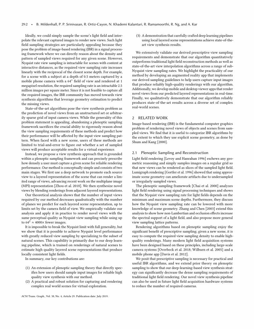
Fig. 8. We plot the performance of our method (with varying number ofplanes D = 8, 16, 32, 64, and 128) compared to light field interpolation fordifferent input view sampling rates (denoted by maximum scene disparitydmax between adjacent input views). Our method can achieve the sameperceptual quality as LFI with Nyquist rate sampling (black dotted line)as long as the number of predicted planes matches or exceeds the under-sampling rate, up to an undersampling rate of 128. At D = 64, this meanswe achieve the same quality as LFI with 642 ≈ 4000× fewer views. We usethe LPIPS [Zhang et al. 2018] metric (lower is better) because we primarilyvalue perceptual quality. The colored dots indicate the point on each linewhere the number of planes equals the maximum scene disparity, whereequality is achieved in our sampling bound (Equation 7). The shaded regionindicates ±1 standard deviation over all 8 test scenes.

view sampling densities such that the maximum disparity betweenadjacent input views ranges from 1 to 256 pixels (a maximum dis-parity of 1 pixel between input views corresponds to Nyquist rateview sampling). We restrict our quantitative comparisons to ren-dered images because a Nyquist rate grid-sampled light field wouldrequire at least 3842 camera views to generate a similar test set,and no such densely-sampled real light field dataset exists to thebest of our knowledge. We report quantitative performance usingthe standard PSNR and SSIM metrics, as well as the state-of-the-artLPIPS [Zhang et al. 2018] perceptual metric, which is based on aweighted combination of neural network activations tuned to matchhuman judgements of image similarity.Finally, our accompanying video shows results on over 60 addi-

tional real-world scenes. These renderings were created completelyautomatically by a script that takes only the set of captured imagesand desired output view path as inputs, highlighting the practicalityand robustness of our method.

6.1 Sampling Theory ValidationOur method is able to render high-quality novel views while signifi-cantly decreasing the required input view sampling density com-pared to standard light field interpolation. Figure 8 shows that ourmethod is able to render novel views with Nyquist level perceptualquality with up to dmax = 64 pixels of disparity between input viewsamples, as long as we match the number of planes in each MPI tothe maximum pixel disparity between input views. We postulate

that our inability to match Nyquist quality from input images with amaximum of 128 pixels of disparity is due to the effect of occlusions.It becomes increasingly likely that any non-foreground scene pointwill be sampled by fewer input views as the maximum disparitybetween adjacent views increases. This increases the difficulty ofdepth estimation and requires the CNN to hallucinate the appear-ance and depth of occluded points in extreme cases where they aresampled by none of the input views.Figure 8 also shows that once our sampling bound is satisfied,

adding additional planes does not increase performance. For exam-ple, at 32 pixels of disparity, increasing from 8 to 16 to 32 planesdecreases the LPIPS error, but performance stays constant from 32to 128 planes. This verifies that for scenes up to 64 pixels of disparity,adding additional planes past the maximum pixel disparity betweeninput views is of limited value, in accordance with our theoreticalclaim that partitioning a scene with disparity variation of D pixelsinto D depth ranges is sufficient for continuous reconstruction.

6.2 Comparisons to Baseline MethodsWe quantitatively (Table 2) and qualitatively (Figure 9) demonstratethat our algorithm produces superior renderings, particularly fornon-Lambertian effects, without the artifacts seen in renderingsfrom competing methods. We urge readers to view our accompany-ing video for convincing rendered camera paths that highlight thebenefits of our approach.

We compare our method to state-of-the-art view synthesis tech-niques as well as view-dependent texture mapping using a globalmesh as proxy geometry. Please refer to Appendix A for additionalimplementation details regarding baseline methods.

Light Field Interpolation (LFI) [Chai et al. 2000]. This baseline isrepresentative of continuous view reconstruction based on classicsignal processing. Following themethod of plenoptic sampling [Chaiet al. 2000], we render novel views using a bilinear interpolationreconstruction filter sheared to the mean scene disparity. Figure 9demonstrates that increasing the camera spacing beyond theNyquistrate results in aliasing and ghosting artifacts when using thismethod.

Unstructured Lumigraph Rendering (ULR) [Buehler et al. 2001].This baseline is representative of view dependent texture mappingwith an estimated global mesh as a geometry proxy. We reconstructa global mesh from all inputs using the screened Poisson surfacereconstruction algorithm [Kazhdan and Hoppe 2013], and use theheuristic Unstructured Lumigraph blending weights [Buehler et al.2001] to blend input images after reprojecting them into the novelviewpoint using the global mesh. We use a plane at the mean scenedisparity as a proxy geometry to fill in holes in the mesh.It is particularly difficult to reconstruct a global mesh with ge-

ometry edges that are well-aligned with image edges, which causesperceptually jarring artifacts. Furthermore, mesh reconstructionoften fails to fill in large portions of the scene, resulting in ghostingartifacts similar to those seen in light field interpolation.

Soft3D [Penner and Zhang 2017]. Soft3D is a state-of-the-art viewsynthesis algorithm that is similar to our approach in that it alsocomputes a local layered scene representation for each input viewand projects and blends these volumes to render each novel view.



Table 2. We quantitatively show that our method outperforms state-of-the-art baselines and specific ablations of our method, across a wide range of inputsampling rates (measured by the maximum pixel disparity dmax between adjacent input views), on a synthetic test set. We display results using the standardPSNR and SSIM metrics (higher is better) as well as the LPIPS perceptual metric [Zhang et al. 2018] (lower is better). The best measurement in each column isbolded. See Sections 6.2 and 6.3 for details on each comparison.

Maximum disparity dmax (pixels)16 32 64 128

Algorithm PSNR ↑ SSIM ↑ LPIPS ↓ PSNR ↑ SSIM ↑ LPIPS ↓ PSNR ↑ SSIM ↑ LPIPS ↓ PSNR ↑ SSIM ↑ LPIPS ↓

Baselines

LFI 26.21 0.7776 0.2541 23.35 0.6982 0.3198 20.60 0.6243 0.3971 18.32 0.5560 0.4665ULR 28.17 0.8320 0.1510 26.43 0.7987 0.1820 24.34 0.7679 0.2311 21.24 0.7062 0.3215Soft3D 34.48 0.9430 0.1345 32.33 0.9216 0.1795 27.97 0.8588 0.2652 23.11 0.7382 0.3979BW Deep 34.18 0.9433 0.1074 34.00 0.9476 0.1128 31.88 0.9192 0.1573 27.59 0.8363 0.2591

Ablations Single MPI 31.11 0.9482 0.1007 29.38 0.9424 0.1111 26.88 0.9250 0.1363 24.20 0.8734 0.1980Avg. MPIs 32.67 0.9560 0.1140 31.34 0.9532 0.1248 29.31 0.9400 0.1423 27.02 0.8999 0.1961Ours 34.57 0.9568 0.0942 34.48 0.9569 0.0954 33.58 0.9530 0.1012 31.96 0.9323 0.1374

However, it uses a hand-crafted pipeline based on classic local stereoand guided filtering to compute each layered representation. Fur-thermore, since classic stereo methods are unreliable for smoothor repetitive image textures and non-Lambertian materials, Soft3Drelies on smoothing their geometry estimation across many (up to25) input views.Table 2 quantitatively demonstrates that our approach outper-

forms Soft3D overall. In particular, Soft3D’s performance degradesmuch more rapidly as the input view sampling rate decreases sincetheir aggregation is less effective when fewer input images view thesame scene content. Our method is able to predict high-quality ge-ometry in scenarios where Soft3D suffers from noisy and erroneousresults of local stereo because we leverage deep learning to learnimplicit priors on natural scene geometry. This is in line with recentwork that has shown the benefits of deep learning over traditionalstereo for depth estimation [Huang et al. 2018; Kendall et al. 2017].Figure 9 qualitatively demonstrates that Soft3D generally con-

tains blurred geometry artifacts due to errors in local depth estima-tion, and that Soft3D’s approach fails for rendering non-Lambertianeffects because their aggregation procedure blurs the specularitygeometry, which changes with the input image viewpoint.

Backwards warping deep network (BW Deep). This baseline sub-sumes recent deep learning view synthesis techniques [Flynn et al.2016; Kalantari et al. 2016], which use a CNN to estimate geometryfor each novel view and then backwards warp and blend nearbyinput images to render the target view. We train a network that usesthe same 3D CNN architecture as our MPI prediction network butinstead outputs a single depth map at the pose of the new targetview. We then backwards warp the five input images into the newview using this depth map and use a second 2D CNN to compositethese warped input images into a single rendered output view. Asshown in Table 2, performance for this method degrades quickly asthe maximum disparity increases. Although this approach producescomparable images to our method for scenes with small disparities(dmax = 16, 32), the renderings suffer from extreme inconsistencywhen rendering video sequences.

BW Deep methods use a CNN to estimate depth separately foreach output viewpoint, so artifacts appear and disappear over only a

few frames, resulting in rapid flickers and pops in the rendered cam-era path. This inconsistency is visible as corruption in the epipolarplots in Figure 9 and can be clearly seen in our supplemental video.Furthermore, backwards warping incentivizes incorrect depth pre-dictions to fill in disocclusions, so BW Deep methods also produceerrors around thin structures and occlusion edges.

6.3 Ablation StudiesWe validate our overall strategy of blending between multiple MPIsas well as our specific blending procedure using accumulated alphaswith the following ablation studies:

Single MPI. The fifth row of Table 2 shows that using only oneMPIto produce new views results in significantly decreased performancedue to the limited field of view represented in a single MPI as well asdepth discretization artifacts as the target view moves far from theMPI reference viewpoint. Additionally, Figure 7 shows an exampleof complex non-Lambertian reflectance that cannot be representedby a single MPI. This ablation can be considered an upper boundon the performance of Zhou et al. [2018], since we use one MPIgenerated by a higher capacity 3D CNN.

Average MPIs. The sixth row of Table 2 shows that blending multi-ple MPI outputs for each novel view without using the accumulatedalpha channels results in decreased performance. Figure 6 visualizesthat this simple blending leads to ghosting in regions that are oc-cluded from the poses of any of the MPIs used for rendering, becausethey will contain incorrect content in disoccluded regions.

7 PRACTICAL USAGEWe present guidelines to assist users in sampling views that enablehigh-quality view interpolation with our algorithm, and showcaseour method’s practicality with a smartphone camera app that guidesusers to easily capture such input images. Furthermore, we imple-ment a mobile viewer that renders novel views from our predictedMPIs in real-time. Figure 9 showcases examples of rendered resultsfrom handheld smartphone captures. Our accompanying video con-tains a screen capture of our app in use, as well as results on over60 real-world scenes generated by an automated script.



Whole scene (Air Plants)

New view path LFI ULR Soft3D BW Deep Blended MPIs (ours)

Whole scene (Pond)


Whole scene (Fern)


Whole scene (T-Rex)


Fig. 9. Results on real cellphone datasets. We render a sequence of new views and show both a crop from a single rendered output and an epipolar slice ofthe sequence. We show 2D projections of the input camera poses (blue dots) and new view path (red line) along the z and y axes of the new view camerain the lower left of each row. LFI fails to cleanly represent objects at different depths because it only uses a single depth plane for reprojection, leading toghosting (leaves in Fern, lily pads in Pond) and depth inconsistency visible in all epipolar images. Mesh reconstruction failures cause artifacts visible inboth the crops and epipolar images for ULR. Soft3D’s depth uncertainty leads to blur, and geometry aggregation across large view neighborhoods resultsin incorrect specularity geometry (brown and blue reflections in Pond). BW Deep’s use of a CNN to render every novel view causes depth inconsistency,visible as choppiness across the rows of the epipolar images in all examples. Additionally, BW Deep selects a single depth per pixel, leading to errors fortransparencies (glass rim in Air Plants) and reflections (Pond). BW Deep also uses backwards warping, which causes errors around occlusion boundaries (thinribs in T-Rex). We urge the reader to refer to our supplemental video for high quality videos of these rendered camera paths and additional discussion.



7.1 Prescriptive Scene Sampling GuidelinesIn a typical capture scenario, a user will have a camera with a fieldof view θ and a world space plane with side length S that boundsthe viewpoints they wish to render. Based on this, we prescribethe design space of image resolutionW and number of images tosample N that users can select from to reliably render novel viewsat Nyquist-level perceptual quality.Section 6.1 shows that the empirical limit on the maximum dis-

parity dmax between adjacent input views for our deep learningpipeline is 64 pixels. Substituting Equation 7:

∆u f

∆xzmin≤ 64. (9)

We translate this into user-friendly quantities by noting that∆u = S/

√N and that the ratio of sensor width to focal length

W∆x /f = 2 tanθ/2:

W√N

≤ 128zmin tan(θ/2)S

. (10)

Using a smartphone camera with a 64◦ field of view, this is simply:

W√N

≤ 80zminS. (11)

Intuitively, once a user has determined the extent of viewpointsthey wish to render and the depth of the closest scene point, they canchoose any target rendering resolutionW and number of images tocapture N such that the ratioW /

√N satisfies the above expression.

7.2 Asymptotic Rendering Time and Space ComplexityWithin the possible choices of rendering resolutionW and numberof sampled views N that satisfy the above guideline, different usersmay value capture time, rendering time, and storage costs differently.We derive the asymptotic complexities of these quantities to furtherassist users in choosing correct parameters for their application.First, the capture time is simply O(N ). The render time of each

MPI generated is proportional to the number of planes times thepixels per plane:

W 2D =W 3S

2√Nzmin tan(θ/2)

= O(W 3N−1/2). (12)

Note that the rendering time for each MPI decreases as the numberof sampled images N increases, because this allows us to use fewerplanes per MPI. The total MPI storage cost is proportional to:

W 2D · N = W 3S√N

2zmin tan(θ/2)= O(W 3N 1/2). (13)

Practically, this means that users should determine their spe-cific rendering time and storage constraints, and then maximizethe image resolution and number of sampled views that satisfytheir constraints as well as the guideline in Equation 10. Figure 10visualizes these constraints for an example user.

Tim

e to render from

one MPI (m

s)Storage space

for all MPIs (G

B)

Fig. 10. Time and storage cost tradeoff within the space of rendering reso-lution and number of sampled views that result in Nyquist level perceptualquality (space above the thick blue curve signifying D = dmax ≤ 64, as inEquation 11). We plot isocontours of rendering time and storage space foran example scene with close depth zmin = 1.0m and target view plane withside length 0.5m, captured with a camera with a 64◦ field of view. We usethe average rendering speed from our desktop viewer and the storage re-quirement from uncompressed 8-bit MPIs. Users can select the point wheretheir desired rendering speed and storage space isocontours intersect todetermine the minimum required number of views and maximum affordablerendering resolution.

(b) Image automatically captured when phone aligns with guide

(a) Grid of guides shows user where to move phone

Equation 8 prescribes

Fig. 11. Equation 7 prescribes a simple sampling bound related only to themaximum scene disparity. We take advantage of the augmented realitytoolkits available in modern smartphones to create an app that helps theuser sample a real scene for rendering with our method. (a) We use built-insoftware to track the phone’s position and orientation, providing samplingguides that allow the user to space photos evenly at the target disparity.(b) Once the user has centered the phone so that the RGB axes align withone of the guides, the app automatically captures a photo.

7.3 Smartphone Capture AppWe develop an app for iOS smartphones, based on the ARKit frame-work, that guides users to capture input views for our view synthesisalgorithm. The user first taps the screen to mark the closest object,and the app uses the corresponding scene depth computed by ARKitas zmin. Next, the user selects the size of the view plane S withinwhich our algorithm will render novel views. We fix the renderingresolution for the smartphone app toW = 500 which therefore fixesthe prescribed number and spacing of required images based onEquation 11 and the definition ∆u = S/

√N . Our app then guides the

user to capture these views using the intuitive augmented realityoverlay shown in Figure 11. When the phone detects that the camerahas been moved to a new sample location, it automatically recordsan image and highlights the next sampling point.



7.4 PreprocessingAfter capturing the required input images, the only preprocessingrequired before being able to render novel views is estimating theinput camera poses and using our trained network to predict an MPIfor each input view. Unfortunately, camera poses from ARKit arecurrently not accurate enough for acceptable results, so we use theopen source COLMAP software package [Schönberger and Frahm2016; Schönberger et al. 2016], which takes about 2-6 minutes forsets of 20-30 input images.We use the deep learning pipeline described in Section 4.1 to

predict an MPI for each input sampled view. On an Nvidia GTX1080Ti GPU, This takes approximately 0.5 seconds for a small MPI(500 × 350 × 32 ≈ 6 megavoxels) or 12 seconds for a larger MPIthat must be output in overlapping patches (1000 × 700 × 64 ≈ 45megavoxels). In total, our method only requires about 10 minutesof preprocessing to estimate poses and predict MPIs before beingable to render novel views at a 1 megapixel image resolution.

With the increasing investment in smartphone AR and on-devicedeep learning accelerators, we expect that smartphone pose estima-tion will soon be accurate enough and on-device network inferencewill be powerful enough for users to go from capturing images torendering novel views within a few seconds.

7.5 Real-Time ViewersWe implement novel view rendering from a singleMPI by rasterizingeach plane from back to front using texture mapped rectangles in 3Dspace, invoking a standard shader API to correctly handle the alphacompositing, perspective projection, and texture resampling. Foreach new view, we determine the MPIs to be blended, as discussed inSection 4.2, and render them into separate framebuffers. We then usea simple fragment shader to perform the alpha-weighted blendingdescribed in Section 4.2. We implement this rendering pipeline asdesktop viewer using OpenGL which renders views with 1000× 700resolution at 60 frames per second, as well as an iOS mobile viewerusing the Metal API which renders views with 500 × 350 resolutionat 30 frames per second. Please see our video for demonstrations ofthese real-time rendering implementations.

7.6 LimitationsA main limitation of our algorithm is that the MPI network some-times assigns high opacity to incorrect layers in regions of ambigu-ous or repetitive texture and regions where scene content movesbetween input images. This can cause floating or blurred patches inthe rendered output sequence (see the far right side of the fern inour video), which is a common failure mode in methods that relyon texture matching cues to infer depth. These artifacts could po-tentially be ameliorated by using more input views to disambiguatestereo matching and by encouraging the network to learn strongerglobal priors on 3D geometry.Another limitation is the difficulty of scaling to higher image

resolutions. As evident in Equations 12 and 13, layered approachessuch as our method are limited by complexities that scale cubicallywith the image width in pixels. Furthermore, increasing the imageresolution requires a CNN with a larger receptive field. This couldbe addressed by exploring multiresolution CNN architectures and

hierarchical volume representations such as octrees, or by predictinga more compact local scene representation such as layered depthimages [Shade et al. 1998] with opacity.

8 CONCLUSIONWe have presented a simple and practical method for view syn-thesis that works reliably for complex real-world scenes, includingnon-Lambertian materials. Our algorithm first promotes each inputimage into a layered local light field representation, then rendersnovel views in real time by blending outputs generated by nearbyrepresentations. We extend traditional layered plenoptic samplinganalysis to handle occlusions and provide a theoretical samplingbound on how many views are needed for our method to renderhigh-fidelity views of a given scene. We quantitatively validate thisbound and demonstrate that we match the perceptual quality ofdense Nyquist rate view sampling while using ≈ 4000× fewer inputimages. Our accompanying video demonstrates that we thoroughlyoutperform prior work, and showcases results on over 60 diverseand complex real-world scenes, where our novel views are renderedwith a fully automated capture-to-render pipeline. We believe thatour work paves the way for future advances in image-based render-ing that combine the empirical performance benefits of data-drivenmachine learning methods with the robust reliability guarantees oftraditional geometric and signal processing based analysis.

ACKNOWLEDGMENTSWe thank the SIGGRAPH reviewers for their constructive comments.The technical video was created with help from Julius Santiago, Mi-los Vlaski, Endre Ajandi, and Christopher Schnese. The augmentedreality app was developed by Alex Trevor.

BenMildenhall is funded by aHertz Foundation Fellowship. PratulP. Srinivasan is funded by an NSF Graduate Fellowship. Ravi Ra-mamoorthi is supported in part by NSF grant 1617234, ONR grantN000141712687, and Google Research Awards. Ren Ng is supportedin part by NSF grant 1617794 and an Alfred P. Sloan FoundationFellowship.

A BASELINE METHODS IMPLEMENTATION DETAILSHere we provide additional implementation details regarding thebaseline comparison methods described in Section 6.2.

Soft3D [Penner and Zhang 2017]. We implemented this algorithmfrom the description provided in the original paper, since no open-source code is currently available. We provide Soft3D’s local stereostage with the same 5 input images used to compute each of ourMPIs, for fair comparison. Next, we aggregate Soft3D’s computedvote volumes across 25 viewpoints, as suggested in their paper for2D view captures. Finally, we compute each rendered novel viewusing the Soft3D volumes corresponding to the same 5 viewpointswhose MPIs we blend between for our algorithm. The guided filterparameters are not specified in the original Soft3D paper, but wefind that best results were obtained using a window size of 8 andϵ = 20 for images with values in the range (0, 255). Please refer toour supplemental video to see results of our Soft3D implementationon a scene shown in the original paper’s video to verify that ourimplementation is of similar quality.



Table 3. Our network architecture. k is the kernel size, s the stride, d thekernel dilation, chns the number of input and output channels for eachlayer, in and out are the accumulated stride for the input and output of eachlayer, input denotes the input of each layer with + meaning concatenation,and layers starting with “nnup” perform 2× nearest neighbor upsampling.

Layer k s d chns in out input

conv1_1 3 1 1 15/8 1 1 PSVsconv1_2 3 2 1 8/16 1 2 conv1_1conv2_1 3 1 1 16/16 2 2 conv1_2conv2_2 3 2 1 16/32 2 4 conv2_1conv3_1 3 1 1 32/32 4 4 conv2_2conv3_2 3 1 1 32/32 4 4 conv3_1conv3_3 3 2 1 32/64 4 8 conv3_2conv4_1 3 1 2 64/64 8 8 conv3_3conv4_2 3 1 2 64/64 8 8 conv4_1conv4_3 3 1 2 64/64 8 8 conv4_2nnup5 128/256 8 4 conv4_3 + conv3_3conv5_1 3 1 1 256/32 4 4 nnup5conv5_2 3 1 1 32/32 4 4 conv5_1conv5_3 3 1 1 32/32 4 4 conv5_2nnup6 64/128 4 2 conv5_3 + conv2_2conv6_1 3 1 1 128/16 2 2 nnup6conv6_2 3 1 1 16/16 2 2 conv6_1nnup7 32/64 2 1 conv6_2 + conv1_2conv7_1 3 1 1 64/8 1 1 nnup7conv7_2 3 1 1 8/8 1 1 conv7_1conv7_3 3 1 1 8/5 1 1 conv7_2

Backwards warping deep network (BW Deep). This baseline is verysimilar to [Kalantari et al. 2016] in overall structure. However, it usesa much larger CNN architecture (same architecture as our method)and takes five images as input rather than four. In addition, since ournetwork is 3D rather than 2D, we can run inference with a variablenumber of planes in the plane sweep volumes rather than fixingD = 100. When generating our quantitative results (Table 2), we setD = dmax, as in our method. We train this baseline with the samesynthetic and real datasets as our network.

Unstructured Lumigraph Rendering (ULR) [Buehler et al. 2001;Gortler et al. 1996]. We use COLMAP’s multiview stereo imple-mentation [Schönberger and Frahm 2016; Schönberger et al. 2016]to generate dense depths and estimate a global triangle mesh ofthe scene from all input images using the screened Poisson surfacereconstruction algorithm [Kazhdan and Hoppe 2013]. For each pixelin a new target view, we implement the heuristic blending weightsfrom [Buehler et al. 2001] to blend input images reprojected usingthe global mesh geometry.

Light Field Interpolation (LFI) [Chai et al. 2000]. This baseline isrepresentative of classic signal processing based continuous viewreconstruction. Following the method of plenoptic sampling [Chaiet al. 2000], for data on a regular 2D grid, we render novel viewsusing a bilinear interpolation reconstruction filter sheared to themean scene disparity. For unstructured real data, we blend together

5 nearby views reprojected to the mean scene disparity, using thesame blending weights as our own method.Note that for methods that depend on a plane sweep volume

(Soft3D, BW Deep, and all versions of our method), we set thenumber of depth planes used in the PSVs to dmax.

B NETWORK ARCHITECTURETable 3 contains a detailed specification of our 3D CNN architecture.All layers except the last are followed by a ReLU nonlinearity andlayer normalization [Lei Ba et al. 2016]. The final layer outputs 5channels. One channel is passed through a sigmoid to generate theoutput MPI’s alpha channel. The other four (along with an all-zerochannel) are passed through a softmax to get five blending weightsfor each voxel which are used to generate the output MPI’s colorchannels, as described in Section 4.1. Restricting one of the softmaxinputs to always be zero makes the function one-to-one rather thanmany-to-one.

REFERENCESMartín Abadi, Ashish Agarwal, Paul Barham, Eugene Brevdo, Zhifeng Chen, Craig

Citro, Greg S. Corrado, Andy Davis, Jeffrey Dean, Matthieu Devin, et al. 2015.TensorFlow: Large-Scale Machine Learning on Heterogeneous Systems. (2015).https://www.tensorflow.org/

Robert Anderson, David Gallup, Jonathan T. Barron, Janne Kontkanen, Noah Snavely,Carlos HernÃąndez, Sameer Agarwal, and Steven M Seitz. 2016. Jump: VirtualReality Video. In SIGGRAPH Asia.

Chris Buehler, Michael Bosse, Leonard McMillan, Steven Gortler, and Michael Cohen.2001. Unstructured Lumigraph Rendering. In SIGGRAPH.

Jin-Xiang Chai, Xin Tong, Sing-Chow Chan, and Heung-Yeung Shum. 2000. PlenopticSampling. In SIGGRAPH.

Gaurav Chaurasia, Sylvain Duchêne, Olga Sorkine-Hornung, and George Drettakis.2013. Depth Synthesis and Local Warps for Plausible Image-based Navigation. InSIGGRAPH.

Qifeng Chen and Vladlen Koltun. 2017. Photographic Image Synthesis With CascadedRefinement Networks. In ICCV.

Shenchang Eric Chen and LanceWilliams. 1993. View Interpolation for Image Synthesis.In SIGGRAPH.

Abe Davis, Marc Levoy, and Fredo Durand. 2012. Unstructured Light Fields. In ComputerGraphics Forum.

Paul Debevec, Camillo J. Taylor, and Jitendra Malik. 1996. Modeling and RenderingArchitecture from Photographs: A Hybrid Geometry-and Image-Based Approach.In SIGGRAPH.

Piotr Didyk, Pitchaya Sitthi-Amorn, William T. Freeman, Fredo Durand, and Woj-ciech Matusik. 2013. 3DTV at Home: Eulerian-Lagrangian Stereo-to-MultiviewConversion. In SIGGRAPH Asia.

John Flynn, Ivan Neulander, James Philbin, and Noah Snavely. 2016. DeepStereo:Learning to Predict New Views From the World’s Imagery. In CVPR.

Steven J. Gortler, Radek Grzeszczuk, Richard Szeliski, and Michael F. Cohen. 1996. TheLumigraph. In SIGGRAPH.

Peter Hedman, Suhib Alsisan, Richard Szeliski, and Johannes Kopf. 2017. Casual 3DPhotography. In SIGGRAPH Asia.

Peter Hedman and Johannes Kopf. 2018. Instant 3D Photography. In SIGGRAPH.Peter Hedman, Julien Philip, True Price, Jan-Michael Frahm, George Drettakis, and

Gabriel Brostow. 2018. Deep Blending for Free-Viewpoint Image-Based Rendering.In SIGGRAPH Asia.

Peter Hedman, Tobias Ritschel, George Drettakis, and Gabriel Brostow. 2016. ScalableInside-Out Image-Based Rendering. In SIGGRAPH Asia.

Po-Han Huang, Kevin Matzen, Johannes Kopf, Narendra Ahuja, and Jia-Bin Huang.2018. DeepMVS: Learning Multi-View Stereopsis. In CVPR.

Nima Khademi Kalantari, Ting-Chun Wang, and Ravi Ramamoorthi. 2016. Learning-Based View Synthesis for Light Field Cameras. In SIGGRAPH Asia.

Michael Kazhdan and Hugues Hoppe. 2013. Screened Poisson Surface Reconstruction.In SIGGRAPH.

Petr Kellnhofer, Piotr Didyk, Szu-Po Wang, Pitchaya Sitthi-Amorn, William Freeman,Fredo Durand, and Wojciech Matusik. 2017. 3DTV at Home: Eulerian-LagrangianStereo-to-Multiview Conversion. In SIGGRAPH.

Alex Kendall, Hayk Martirosyan, Saumitro Dasgupta, Peter Henry, Ryan Kennedy,Abraham Bachrach, and Adam Bry. 2017. End-to-End Learning of Geometry andContext for Deep Stereo Regression. In ICCV.


https://www.tensorflow.org/


Diederik P. Kingma and Jimmy Ba. 2015. Adam: A Method for Stochastic Optimization.In ICLR.

Johannes Kopf, Fabian Langguth, Daniel Scharstein, Richard Szeliski, and MichaelGoesele. 2013. Image-Based Rendering in the Gradient Domain. In SIGGRAPH Asia.

Philippe Lacroute and Marc Levoy. 1994. Fast Volume Rendering Using a Shear-WarpFactorization of the Viewing Transformation. In SIGGRAPH.

Douglas Lanman, Ramesh Raskar, Amit Agrawal, and Gabriel Taubin. 2008. ShieldFields: Modeling and Capturing 3D Occluders. In SIGGRAPH Asia.

Jimmy Lei Ba, Jamie Ryan Kiros, and Geoffrey E. Hinton. 2016. Layer Normalization.In arXiv:1607.06450.

Marc Levoy and Pat Hanrahan. 1996. Light Field Rendering. In SIGGRAPH.Leonard McMillan and Gary Bishop. 1995. Plenoptic Modeling: An Image-Based

Rendering System. In SIGGRAPH.Rodrigo Ortiz-Cayon, Abdelaziz Djelouah, and George Drettakis. 2015. A Bayesian

Approach for Selective Image-Based Rendering using Superpixels. In InternationalConference on 3D Vision (3DV).

Ryan S. Overbeck, Daniel Erickson, Daniel Evangelakos, Matt Pharr, and Paul Debevec.2018. A System for Acquiring, Processing, and Rendering Panoramic Light FieldStills for Virtual Reality. In SIGGRAPH Asia.

Eric Penner and Li Zhang. 2017. Soft 3D Reconstruction for View Synthesis. In SIG-GRAPH Asia.

Thomas Porter and Tom Duff. 1984. Compositing Digital Images. In SIGGRAPH.Weichao Qiu, Fangwei Zhong, Yi Zhang, Siyuan Qiao, Zihao Xiao, Tae Soo Kim, Yizhou

Wang, and Alan Yuille. 2017. UnrealCV: Virtual Worlds for Computer Vision. InACM Multimedia Open Source Software Competition.

Johannes Lutz Schönberger and Jan-Michael Frahm. 2016. Structure-from-MotionRevisited. In CVPR.

Johannes Lutz Schönberger, Enliang Zheng, Marc Pollefeys, and Jan-Michael Frahm.2016. Pixelwise View Selection for Unstructured Multi-View Stereo. In ECCV.

Jonathan Shade, Steven J. Gortler, Li wei He, and Richard Szeliski. 1998. Layered depthimages. In SIGGRAPH.

Heung-Yeung Shum and Sing Bing Kang. 2000. A Review of Image-Based RenderingTechniques. In Proceedings of Visual Communications and Image Processing.

Sudipta Sinha, Johannes Kopf, Michael Goesele, Daniel Scharstein, and Richard Szeliski.2012. Image-Based Rendering for Scenes with Reflections. In SIGGRAPH.

Shuran Song, Fisher Yu, Andy Zeng, Angel X Chang, Manolis Savva, and ThomasFunkhouser. 2017. Semantic Scene Completion from a Single Depth Image. In CVPR.

Pratul P. Srinivasan, Tongzhou Wang, Ashwin Sreelal, Ravi Ramamoorthi, and Ren Ng.2017. Learning to Synthesize a 4D RGBD Light Field from a Single Image. In ICCV.

Rahul Swaminathan, Sing Bing Kang, Richard Szeliski, Antonio Criminisi, and Shree K.Nayar. 2002. On the Motion and Appearance of Specularities in Image Sequences.In ECCV.

Gordon Wetzstein, Douglas Lanman, Wolfgang Heidrich, and Ramesh Raskar. 2011.Layered 3D: Tomographic Image Synthesis for Attenuation-based Light Field andHigh Dynamic Range Displays. In SIGGRAPH.

Gordon Wetzstein, Douglas Lanman, Matthew Hirsch, and Ramesh Raskar. 2012. Ten-sor Displays: Compressive Light Field Synthesis using Multilayer Displays withDirectional Backlighting. In SIGGRAPH.

Bennett Wilburn, Neel Joshi, Vaibhav Vaish, Eino-Ville Talvala, Emilio Antunez, AdamBarth, Andrew Adams, Marc Levoy, and Mark Horowitz. 2005. High PerformanceImaging Using Large Camera Arrays. In SIGGRAPH.

Daniel N. Wood, Daniel I. Azuma, Ken Aldinger, Brian Curless, Tom Duchamp, David H.Salesin, and Werner Stuetzle. 2000. Surface Light Fields for 3D Photography. InSIGGRAPH.

GaochangWu, Mandan Zhao, LiangyongWang, Qionghai Dai, Tianyou Chai, and YebinLiu. 2017. Light Field Reconstruction Using Deep Convolutional Network on EPI. InCVPR.

Henry Wing Fung Yeung, Junhui Hou, Jie Chen, Yuk Ying Chung, and Xiaoming Chen.2018. End-to-End Learning of Geometry and Context for Deep Stereo Regression.In ECCV.

Cha Zhang and Tsuhan Chen. 2003. Spectral Analysis for Sampling Image-BasedRendering Data. In IEEE Transactions on Circuits and Systems for Video Technology.

Richard Zhang, Phillip Isola, Alexei A Efros, Eli Shechtman, and Oliver Wang. 2018.The Unreasonable Effectiveness of Deep Features as a Perceptual Metric. In CVPR.

Zhoutong Zhang, Yebin Liu, and Qionghai Dai. 2015. Light Field from Micro-BaselineImage Pair. In CVPR.

Tinghui Zhou, Richard Tucker, John Flynn, Graham Fyffe, and Noah Snavely. 2018.Stereo Magnification: Learning View Synthesis using Multiplane Images. In SIG-GRAPH.


Documents

Local Light Field Fusion: Practical View Synthesis …Local Light Field Fusion: Practical View Synthesis with Prescriptive Sampling Guidelines BEN MILDENHALL∗, University of California,