Liquidity and Asset Pricing: Evidence on the Role of ...finance.bi.no/~bernt/wps/holding_period/holding_period_paper_mar... · Liquidity and Asset Pricing: Evidence on the Role of

Liquidity and Asset Pricing: Evidence on the Role ofInvestor Holding Period

Randi Næs and Bernt Arne Ødegaard∗

March 2009

Abstract

We use data on actual holding periods for all investors in a stock market over a10-year period to investigate the links between holding periods, liquidity, and assetreturns. Microstructure measures of liquidity are shown to be important determi-nants of the holding period decision of individual investors. Average holding periodsdiffer across different investor types. Turnover is an imperfect proxy for holding pe-riod. While both turnover and spread are related to stock returns, holding periodis not.

Keywords: Market microstructure, Liquidity, Holding period

JEL Codes: G10, G11, G12

∗Randi Næs is at the Ministry of Trade and Industry. Bernt Arne Ødegaard is at the Univer-sity of Stavanger, BI Norwegian School of Management and Norges Bank. Correspoding author:Bernt Arne Ødegaard, University of Stavanger, NHS/IØL, NO-4036 Stavanger, (+47) 51 83 37 87,[email protected] The views expressed are those of the authors and should not be interpretedas reflecting those of Norges Bank. We are grateful for comments from Trond Døskeland, C. EdwardFee, Stuart Hyde, Brett C. Olsen and Petter Osmundsen, from conference participants at the ThirdAnnual Central Bank Microstructure Conference at the Hungarian Central Bank, the FIBE 2008, Mid-western Finance Association (MFA) 2008, European Winter Finance Summit 2008 and 2008 EuropeanFinance Association conferences, and from seminar participants in Norges Bank and at the Universityof Stavanger.

1

Liquidity and Asset Pricing: Evidence on the Role of InvestorHolding Period

Abstract

We use data on actual holding periods for all investors in a stock market over a10-year period to investigate the links between holding periods, liquidity, and assetreturns. Microstructure measures of liquidity are shown to be important determi-nants of the holding period decision of individual investors. Average holding periodsdiffer across different investor types. Turnover is an imperfect proxy for holding pe-riod. While both turnover and spread are related to stock returns, holding periodis not.

Keywords: Market microstructure, Liquidity, Holding period

JEL Codes: G10, G11, G12

Introduction

Numerous empirical studies find that liquidity matters for asset returns. On the theoreti-cal side, however, there is little agreement on what aspects of liquidity can generate largecross-sectional effects in asset returns. A number of theoretical models use the conceptof expected holding period to link liquidity to asset prices.1 So far, it has been hard toinvestigate these theories empirically. While some attempts have been made, they allsuffer from lack of data on actual holding periods. Instead they rely on proxies of investorholding periods constructed from data on turnover. Even though a high-turnover stocknecessarily has many of the stock’s investors buying and selling the stock, it is by nomeans certain that all owners of the stock have short holding periods.2 The core of thisproblem is that turnover is a characteristic of a stock, while holding period is a decisionmade by individual investors.

In the present paper, we analyze the relationship between holding periods, liquidityand asset prices using data on actual holding periods. The source of our contribution isaccess to the complete holdings for all investors at the Oslo Stock Exchange (OSE) overa 10-year period.3 Our ability to measure holding periods from data on actual tradingdecisions at the level of individual investors, observed over a substantial period of time,

1Amihud and Mendelson (1986) is an early model where the expected holding period enters.2The stock may have a group of very long holding period owners, but high turnover among the

remaining investors.3Current evidence on investor trading activity is largely based on small samples of investors, such as

the the single broker customers of Barber and Odean (2000).

2

is quite exceptional. The only other papers which considers some of the same issues withsimilar data are Kyrolainen and Perttunen (2006), using data from Finland, and Diasand Ferreira (2005), using a sample of Portuguese investors. Both papers look at theholding period decisions of individual investors using datasets which are of shorter timeperiods, and, in the case of the Portuguese data, less complete, and neither of the papersattempts to move beyond the behaviour of individual investors to the wider implicationsof holding periods for the whole market.

In our work we look at three issues. First, we describe individual holding perioddecisions, and evaluate the determinants of these decisions. The typical holding periodis found to be three quarters of a year, but the probabilities of liquidating an equityposition, conditional on the length of time the ownership has lasted, show considerabletime variation. Typical measures of liquidity, such as the bid/ask spread and turnover,are important determinants of individual holding period decisions. We also find cleardifferences in average holding periods across investor types.

Second, we ask to what degree typical proxies of holding period measure actual holdingperiods. We both compare actual holding period estimates to alternatives provided in theliterature, and investigate the extent to which, in the cross-section of equities, holdingperiods and liquidity measures covary. Relative to existing evidence, holding periodsseem shorter than previously thought. This is due to the fact that the distribution ofactual holding periods is very skewed, at the same time as the distribution of turnoveracross stocks is skewed. Our estimate of the median holding period from turnover data isclose to the mean actual holding period of around 2 years, a significantly higher numberthan the median actual holding period of 0.75 years. To investigate the consistency ofholding period and liquidity measures, we construct a measure of average holding periodat the stock level. As expected, the average holding period measure is positively relatedto spreads and negatively related to turnover. However, the correlations are surprisinglylow.

Third, we investigate links between holding periods and asset prices. There are severaltheoretical arguments linking these. In the Amihud and Mendelson (1986) model thereis an indirect link, where long term investors choose high spread stocks, and Amihud andMendelson document a link between spreads and returns. Information based arguments,such as those in Yan and Zhang (2008), imply returns differences if long and short terminvestors are differently informed. To investigate these issues we therefore perform anumber of cross-sectional asset pricing tests involving measures of actual holding periods.We find that while the average holding period measure is related to other measures ofliquidity in the expected directions, it does a worse job in explaining the cross-section ofstock returns than more standard measures of liquidity.

3

The paper is structured as follows. In Section 1 we briefly summarize the paperson holding periods, liquidity and asset pricing that are most relevant in our setting.Section 2 describes the market and the data set. In Section 3 we investigate the individualowners’ holding period decisions. In Section 4 we look at how our actual holding periodscompare to alternative proxies for holding periods suggested in the literature. We alsorelate holding periods to standard measures of liquidity. In Section 5 we compare theasset pricing implications of holding period measures and liquidity measures. Section 6concludes.

1 Literature

The standard way of incorporating market frictions into asset pricing models is to assumethat trading involves some exogenous trading cost (or illiquidity cost).4 This impliesthat investors’ expected holding period is crucial for the effect of illiquidity on requiredreturns, i.e. the more often investors plan to trade, the more important are the tradingcosts. The importance of illiquidity costs therefore depends on the assumed structureof holding periods in a model. The simplest assumption possible is that the expectedholding period is exogenous and identical for all investors. Assuming risk neutrality,these assumptions imply that the required return on assets is equal to the risk-free rateplus the per period percentage transaction cost, see Amihud et al. (2005).5

In the model of Amihud and Mendelson (1986), risk-neutral investors are assumedto have different exogenous holding periods and limited capital. These assumptionsintroduce a clientele effect into the solution whereby investors with long expected holdingperiods select stocks with high trading costs. The required return will then differ fordifferent classes of investors, and the expected gross return becomes an increasing andconcave function of the relative transaction cost. Amihud and Mendelson find empiricalsupport for this hypothesis using spreads and stock returns from the NYSE over the1961-80 period.6

4In fact, even the simple assumption that illiquidity reflects exogenous trading costs seriously com-plicates standard asset pricing models. This is because it precludes the existence of a pricing kernel thatcan price all securities. Explicit pricing rules can then only be derived under special assumptions, seeAmihud, Mendelson, and Pedersen (2005).

5Risk neutrality implies that all assets are identical. Huang (2003) extends this analysis and studiesthe premium for liquidity risk assuming exogenous holding periods and risk-averse investors.

6Several other papers attempt to test the model using turnover as a proxy for holding period. Atkinsand Dyl (1997) find evidence consistent with the spread-holding period relationship using the inverseof turnover as a proxy for the average holding period. Datar, Naik, and Radcliffe (1998) show thatturnover is negatively related to stock returns in the cross-section, while Hu (1997) finds support forboth an increasing and concave return-holding period relationship using data on returns and turnoverfrom the Tokyo Stock Exchange. In the empirical test of their liquidity-adjusted CAPM, Acharya andPedersen (2005) find a significant effect on prices from liquidity cost, also using turnover as proxy for

4

On the other hand, more realistic models with endogenous holding periods and risk-averse investors find that an exogenous liquidity cost has only miniscule effects on the levelof asset returns. In a continuous-time model with exogenous asset prices, Constantinides(1986) shows that the optimal investment policy for risk-averse investors involves a trade-off between high trading costs from frequent portfolio rebalancing and utility costs fromhaving a suboptimal asset allocation. While trading costs have a first-order effect on thedemand for the asset, they only have a second-order effect on equilibrium asset returns.Vayanos (1998) extends this analysis to a general equilibrium model with endogenousholding periods. A calibration of his model gives a similar result; the effects of tradingcosts on equilibrium asset returns are small. Hence, we have the intriguing result thatmore realistic models assuming risk aversion and endogenous holding periods seem to doconsiderably worse in explaining empirical findings than less realistic models with riskneutrality and exogenous holding periods.

Huang (2003) notes that an important reason behind the discrepancy between the-ory and empirical findings regarding the effect of liquidity on asset prices is that assetpricing models in general cannot explain the observed high market trading volume. Thestrong dependence of liquidity premia on investor holding periods implies that theoriesthat cannot account for observed high trading volume cannot explain observed liquid-ity premia either. In a model with uncertain exogenous holding periods, Huang showsthat the premium for liquidity risk can be large if investors face liquidity shocks and areconstrained from borrowing.7

Another and potentially related explanation is the restriction in asset pricing modelsthat liquidity costs are exogenous. The market microstructure literature divides marketfrictions into asymmetric information costs and coordination costs (inventory risk andsearch problems), and shows that prices can diverge from long-term equilibrium valuesdue to strategic trading behavior of investors. Thus, models that do not specify theultimate source of trading cost differences cannot really explore how a full equilibriumwill look like. For instance, it is not obvious that investors with long expected holdingperiods will select stocks with high trading costs since holding “long term” stocks reducesthe value of the option to sell the stocks early.

While much of our analysis is inspired by models starting from the Amihud andMendelson (1986) analysis, there are alternative formulations which may induce a linkbetween holding periods and returns. In a recent paper, Yan and Zhang (2008) start withthe premise of differently informed long term and short term investors, and show thatthis has implications for returns.

investors’ average holding periods.7Introducing additional motives for trade, Getmansky, Lo, and Makarov (2004) also find that the

liquidity premium can be large when investors have high frequency trading needs.

5

Obviously, more knowledge about how and why expected holding periods differ amonginvestors is highly valuable, and our paper significantly adds to our knowledge on this.There are two papers that are closely related to our analysis. Kyrolainen and Perttunen(2006) looks at a dataset of Finnish investors and Dias and Ferreira (2005) at a datasetof Portuguese investors. We expand on the analysis in these papers in a number ofways. First, while both these papers find some of the results we find on the behaviourof individual investors, neither of them go on to consider the wider implications of theirfindings for the cross-section of stock returns. Second, we have a more comprehensivesample of investors over a longer time period. Relative to the analysis of Kyrolainen andPerttunen (2006) we use a more correct method of analysis, based on duration analysis,which is also used in Dias and Ferreira (2005).

2 Market and data

The firms in the sample are listed on the Oslo Stock Exchange (OSE), which is a mod-erately sized exchange by international standards. In 1997 (about the midpoint of oursample), the 217 listed firms had an aggregate market capitalization which ranked theOSE twelfth among the 21 European stock exchanges for which comparable data areavailable. The number of companies on the exchange has increased from 141 in 1989 to212 in 2003.8

This paper uses monthly data from the Norwegian equity market for the period1992:12 to 2003:6. From the Norwegian Central Securities Registry (VPS) we havemonthly observations of the equity holdings of the complete stock market. At eachdate we observe the number of stocks owned by every owner. Each owner has a uniqueidentifier which allows us to follow the owners’ holdings over time. For each owner thedata include a sector code that allows us to distinguish between such types as mutualfund owners, financial owners (which include mutual funds), industrial (nonfinancial cor-porate) owners, private (individual) owners, state owners and foreign owners. In additionto this anonymous data set, we use public reports on individual owners’ inside transac-tions to construct measures of insider ownership.9 A third data source is the Oslo StockExchange Data Service (OBI). This source provides stock prices and accounting data.Finally, we use interest rate data from Norges Bank, the Central Bank of Norway.

8For some information about the structure of the Norwegian stock market we refer to Bøhren andØdegaard (2000, 2001), and Næs, Skjeltorp, and Ødegaard (2008).

9For more details on this insider trading data see Eckbo and Smith (1998) and Bøhren and Ødegaard(2001).

6

3 What affects holding periods for individual investors?

In this section, we use duration analysis to describe actual holding periods and to studywhat variables might affect holding period decisions. By investigating whether the spreadis an important determinant of investors’ holding periods, we perform a direct test of thespread-holding period relationship in Amihud and Mendelson (1986).

3.1 Duration analysis

The econometric framework suited for analyzing questions about the length of time aninvestor chooses to keep his or her stake in a company, and what economic factors affectthis decision, is duration (or survival) analysis. In duration analysis, one models thedecision to terminate a relationship. In our setting, termination is the decision to liquidatean equity holding in a company.10

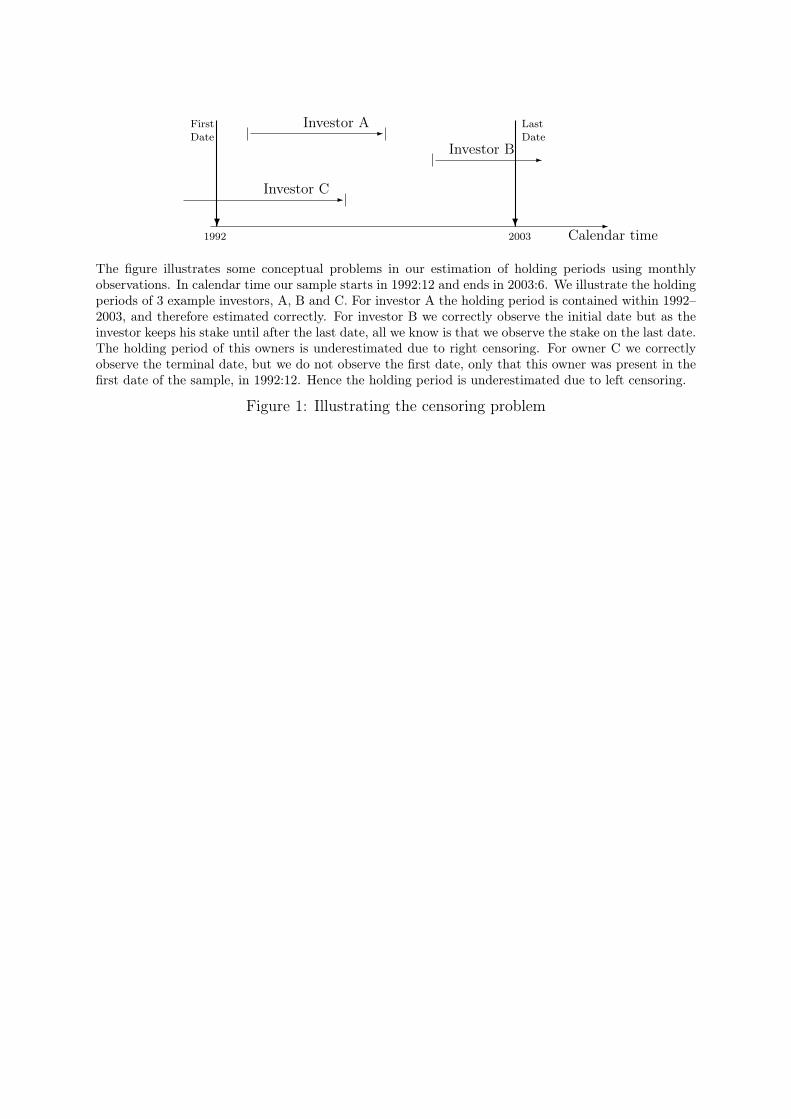
Duration analysis is the preferable method for analyzing holding period decisionsbecause it is designed to alleviate the problem of censoring. In our setting, the censoringproblem stems from the fact that we only observe investors for a limited period of time.Figure 1 illustrates the problem. Of the investors illustrated in the figure, it is onlythe holding period of investor A which will be measured correctly. The holding period ofinvestor B will be right censored ; all we see is that the investor was present at the last dateand we do not know the final termination date. For investor C we correctly observe theterminal date, but we do not observe when the relationship is initiated, which is termedleft censoring. Duration analysis involves the estimation of the probability distributionof the termination decision, taking the censoring problem into account.

This probability distribution of the termination decision can be characterized in anumber of ways, for example by the survival function: the probability of surviving beyonda given date, or the hazard function: the probability of termination, conditional on havingsurvived so far. The most common way of characterizing the probability distribution isthrough the hazard function. When we want to ask what factors affect duration, this isdone by measuring a factor’s contribution to the hazard function.

10In economics, duration models are used on e.g. labor market data to analyze determinants of thetime spent unemployed, in which case the pertinent termination is movement between employment andunemployment, see Lancaster (1979) and Nickell (1979) for examples and Kiefer (1988) and van den Berg(2001) for surveys.

7

3.2 Estimated hazard and survival functions

We apply duration analysis to the holding periods of individual investors using monthlydata for all investors at the OSE over the period 1992-2003.11 To reduce noise, investorswith less than five hundred shares are removed from the sample. Thus, we count as ini-tiation the first time an investor is observed holding 500 or more shares, and terminationwhen he or she reduces the stake to less than 500 shares.12 This leaves about 1.4 millionobservations of investor-company durations.13 In Table 1, we show mean and medianholding periods for all owners and for owners grouped by investor type, i.e. financial,foreign, nonfinancial, individual and state investors. The numbers in the table illustratesome very interesting regularities in the data. For our purposes the most interestingnumber is the median, which is the holding period of the typical investor. Looking at allowners in the market, we find that the typical investor holds a position for 0.75 years.The median holding period varies significantly by type of investor, however. The mostpatient investors are private individuals, who hold their positions for 0.83 years, while thetypical corporate investor, be it financial or nonfinancial, holds a position for only half ayear. Note also that the mean holding periods are considerably higher than the medianholding periods. Overall, the estimated mean holding period is close to 2 years, which ismore than twice the length of the median holding period.14 These findings clearly illus-trate the skewed nature of the holding period distribution, where a few very long-terminvestors inflate the mean holding period. This feature of the data points to the need touse duration analysis to explicitly model the full distribution of holding periods, to whichwe now turn.

In Figure 2, we show the estimated survival- and hazard functions for the completesample of investors. From the survival function, shown in the left panel of the figure, wecan read the median holding period of 0.75 from the point where the survival functioncrosses the 0.5 line. Other interesting properties of holding periods are, however, betterillustrated by the hazard function shown in the right panel of the figure.15 If the proba-

11In survival analysis terms, our data set is a an example of spell data, where there is interval censoringsince we only observe once every month, and there are some (identified) spells which may be left or rightcensored. While the interval censoring could be analyzed using discrete methods, we have for simplicitychosen to approximate the survival function as continuous.

12At the Oslo Stock Exchange, the typical minimal trading lot is 100 shares. Requiring five times theminimum lot size seems like a conservative lower limit on who is a “substantial” owner. Looking only atcomplete sellouts of stakes is of course a simple definition of termination. One could think of alternatives,such as a stake decrease by a given percentage.

13An investor can have several durations, both in the same and in other stocks.14The estimate of 1.97 is adjusted for the censoring of data by extrapolation. Without censoring

adjustment the estimate is 1.86.15The hazard functions that follow are estimated using a Weibull probability distribution assumption.

We have also looked at alternatives, such as a Cox specification. The results are robust to these alternativeprobability distributions.

8

bilities of liquidating an equity position, conditional on the length of time the ownershiphas lasted, are time independent, the hazard function will be flat. This is clearly notthe case for our sample. Instead, we see a systematic time variation. The conditionalprobability of exit starts around 0.45, increasing to a maximum slightly above 0.5 around1 year, and then decreases steadily, reaching 0.2 after 8 years, and keeps decreasing. Thedecreasing part of the curve after 1 year means that if an owner has held the stock for oneyear, he or she is less and less likely to terminate as time passes. The high probability ofexit at the short horizon is the prime contributor to stock turnover. Over the same timeperiod, the average annual stock turnover was about 60%.16

3.3 Determinants of the hazard function

Having described holding periods, we now turn to investigating what variables mightaffect the holding period decision. Duration analysis lets us ask this question by esti-mating the effect of a variable on the hazard function. In the standard specification ofduration analysis, the hazard function is a constant function of the explanatory variables.We use time-varying explanatory variables such as firm size, stock volatility and spreadin our analysis. To implement estimation we use the observed values of an explanatoryvariable at the time when a stake is first acquired as the input to the estimation. In eco-nomic terms this can be viewed as the holding period decision being based on observablevariables when the initial stake is acquired.

By including spread as an explanatory variable, we perform a direct test of the spread-holding period relationship in Amihud and Mendelson (1986). Earlier empirical analysis,such as Atkins and Dyl (1997), tests this relationship using turnover as a proxy forholding period. Our paper improves on this analysis in two respects. First, we basethe analysis on actual holding periods at the individual investor level. Second, we usethe correct econometric framework for testing. The question of whether liquidity affectsholding periods should be asked by testing whether the liquidity at the time when thestock position is entered into affects the hazard function for holding periods. In theiranalysis, Amihud and Mendelson use spread as their liquidity measure. In our analysiswe consider both spread and turnover as liquidity measures.

In Amihud and Mendelson (1986), investors coming to the market have different ex-pected holding periods. One rationale for this assumption could be that different groups

16It should be mentioned that there are some problems with the analysis at the very short end, inducedby the fact that the minimum possible observation of holding period is one month. Since we only havemonthly observations of holdings our minimal estimate of holding period is one month, found when wehave only two consecutive observations of stock holdings. Cases where we only have one observation,with no observation of holdings for that owner either the month prior or the month after, are roundeddown to a duration of zero. Zero durations are not used in the estimation.

9

of investors have distinctly different trading motives, for instance long-term pension sav-ing versus short-term speculation. To account for these possibilities we consider investortype as an explanatory variable. Investor type is included in our analysis in two differ-ent ways. First, we use dummy variables for investor type in the estimation. However,since we are estimating a nonlinear relationship, dummy variables may not capture allthe relevant information. We therefore also perform the analysis separately for the fivedifferent owner types.

It is also possible that an investor’s planned holding period is influenced by the sizeof the investment. We therefore include investment amount as an explanatory variable.Since we only have monthly observations of holdings, we estimate the investment amountas the stock price at the end of the month multiplied by the number of shares. To avoidnumerical difficulties we use the log of the investment.

In panel A of Table 2 we show the results from estimating the contributions to thehazard function of the investor-specific variables described above as well as two liquiditymeasures, relative spread (columns 2-3) and turnover (columns 4-5). The coefficients inthe table measure contributions to the hazard function. Note here the interpretation ofthese coefficients: If a coefficient equals one, it does not contribute. A coefficient lessthan one lowers the conditional probability of exit, while a coefficient greater than oneincreases the probability of exit.

Let us first look at the estimated relationship between spread and holding period.As seen in the table, the coefficient is significantly below one. High spread decreasesthe probability of exit. We therefore confirm the posited relationship between spreadand holding period. Stocks with high spreads tend to have owners with longer holdingperiods. Similarly, stocks which have recently experienced high turnover tend to haveowners with shorter holding periods looking forward. The other explanatory variablesin the regressions are all significant. The amount invested has a negative effect on thehazard function. This means that larger owners tend to have longer holding periods.The analysis also shows clear differences across investor types in average holding periods.Financial owners are the shortest term, while individual owners have the longest holdingperiods. Foreign and non-financial (corporate) owners have holding periods in betweenthese two extremes.

In the estimation above, we only use investor-specific information and liquidity mea-sures as explanatory variables. However, other properties of a stock may also be relevantfor holding period decisions. To account for this, we add a few firm-specific variables tothe analysis. Following Atkins and Dyl (1997), we include logs of stock volatility andfirm size as possible determinants of holding period. In panel B of Table 2 we show theresults when these two variables are added for two different analyzes of determinants of

10

the hazard function, one using the spread as a liquidity measure, the other using turnover.In both specifications, volatility and firm size are significantly related to holding period.The holding periods tend to be shorter in firms with high volatility and large size. Notealso that foreign ownership no longer is significant. This is probably because it is corre-lated with firm size. However, for our purposes the most important observation is thatthere is still a significant relation between liquidity and holding period. Ex ante liquidityaffects realized holding periods.

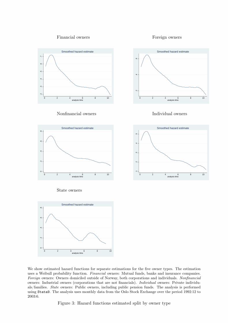
The dummy variables for investor type show significant differences across owner types;however, as noted above, simple dummy variables may not capture differences in theshape of the hazard function for the different owner types. We therefore redo the hazardfunction estimation for each of the five subsamples. Figure 3 and Table 3 show the results.There are some differences across owner types worth pointing out. The fact that financialand nonfinancial owners are relatively more impatient is seen by the higher values of thehazard function at the short end. Another interesting feature is the difference in thecontribution of the investment amount across owner types. For individual owners, wefind that the larger the initial investment the longer the holding period. For all the otherowner types this relation is opposite. Larger investments tend to lead to shorter holdingperiods. This can be due to the importance of the investment in the portfolio of individualinvestors. While there are some differences across owner type, there are no differences inthe relationship of most interest for our purposes. We see that ex ante liquidity is stillan important determinant of future holding periods.

To conclude, there are two important results in this section that add to our knowledgeof the link between holding periods and stock liquidity. First, we show that the conditionalprobability distribution of holding periods has a clear time variation. Most owners areshort term; the typical owner keeps the position for three quarters of a year. But there isalso a group of very long-term owners. In our sample, about 10% of the owners kept theirpositions for the whole sample period of ten years. Second, we show that stock liquidity,be it measured by spread or turnover, influences holding period decisions.

4 Proxies of holding periods

In this section we use our data on holding periods to shed light on the relationshipbetween holding period and different measures of liquidity. First, we investigate whetherthe inverse of turnover is a good proxy for holding period as suggested by Atkins and Dyl(1997). We show that the proxy seriously overstates actual holding periods of individualinvestors. Second, we consider ranking of the cross-section of equities by measures ofholding periods, and ask to what extent this ranking is related to rankings by standard

11

liquidity measures. To perform such an analysis it is necessary to construct a measurethat aggregates individual holding periods into a measure of holding periods at the stocklevel.

4.1 Estimating holding period from stock turnover

Atkins and Dyl (1997) use the inverse of annual turnover as an estimate of the averageholding period of a firm’s investors, i.e.

Holding Periodt =Shares outstanding in year tNo of shares traded in year t

and argue that this is a reasonable approximation of holding periods when investigatingthe relationship between transactions costs and investors’ holding periods. As we shall see,however, the validity of this argument depends crucially on the distributional propertiesof actual holding periods.

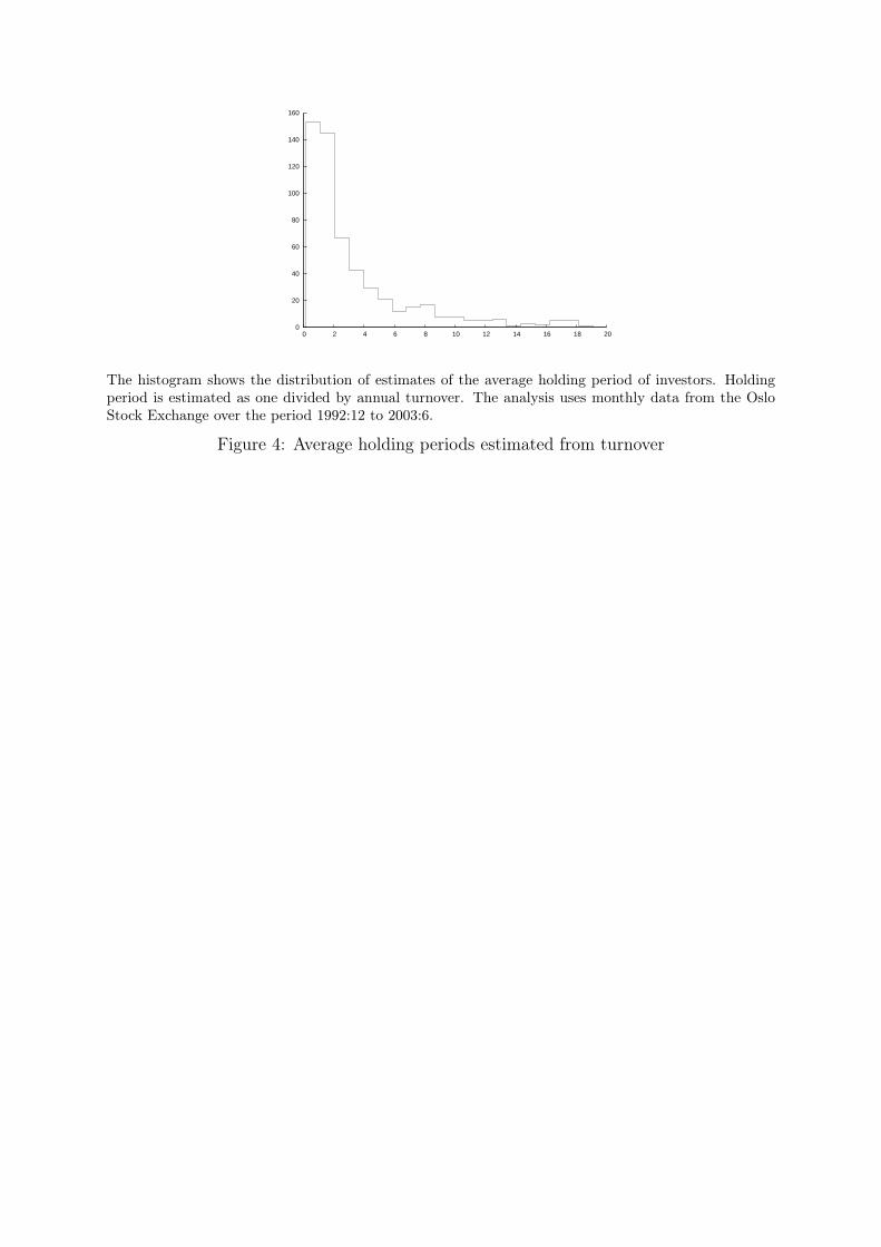
Atkins and Dyl estimate average holding periods from a sample of US firms listedon NYSE and Nasdaq. Table 4 shows the results of the estimation and compare themwith similar estimates for Norway. Estimating average holding period from turnover, wefind an average across stocks of 3.33 years. However, as illustrated by the histogram infigure 4, the mean of this distribution is seriously pushed upward by a few very largeestimates. The median of 1.96 is therefore a much better estimate of the typical holdingperiod estimated from turnover. When we relate this result to the estimation of mean andmedian holding periods based on individual owners, we note the following. The estimateof the typical holding period based on turnover (1.97) hits the mean holding periodfor individual investors uncannily on the spot (1.96). The two estimates are thereforeconsistent with each other. However, from our data on actual holding periods, we knowthat this estimate of the mean holding period is seriously inflated by a few long-terminvestors. Put differently, the estimate based on turnover is not able to distinguish themore complex dynamics of holding periods we find from the data for individual investors,where we have a large group of short-term, impatient investors, and a smaller group ofmuch longer term, patient investors. Thus, we cannot detect the typical holding periodof 0.75 years using turnover data.

In the next section, we investigate to what degree data on individual owners’ holdingperiods give additional, and different, information, than what we can find from turnover.

12

4.2 What is the relationship between actual holding periods and

liquidity measures?

In this subsection, we shift focus from the holding period of individual owners to holdingperiods as an aggregate property of all the owners of a stock. The impetus for theseanalyzes comes from the empirical asset pricing evidence of a positive relationship betweenasset prices and microstructure measures of liquidity. If liquidity is an exogenous tradingcost, as assumed in the theoretical asset pricing literature, then the link between liquidityand asset prices must be one of cost compensation. This cost compensation will vary withinvestors’ expected holding period. We therefore want to investigate whether liquiditycovaries with holding periods as such theories suggest. To investigate this we need ameasure of average holding period at the stock level.

4.2.1 An index of average holding period at the stock level

To get a measure of holding period that we can relate to measures of stock liquidity,that are measured over short time intervals, we construct a holding period index. Themeasure is constructed as a “snapshot”, where we take the owners at a given date, measurethe holding period for each owner, and aggregate these individuals into one measure perstock. To lessen time series overlap, we truncate the measurement interval to one year ata time.17

Figure 5 illustrates our method for creating the index. At a given date t we use datafor the holdings in the previous year. We take all owners with an equity stake at timet.18 In the figure it means that we use owners 1, 3 and 4. Owner 2 has sold her stake 6months earlier, and is not present in the company at date t. The holding period indexfor each owner is the holding period in fractions of a year. The index for the company isa weighted sum of the individual owners’ indices. In the example in figure 5 the holdingperiod index is

hpi = w11 + w37

12+ w4

3

12,

where wi is the weight for owner i. The weight for each individual can vary. If we wantto put more weight on the large owners we use value weights where the fraction of thecompany held by each owner at time t is the weight. This index is termed hpi(vw). If weare more interested in the typical owner we use equal weights 1/n, where n is the numberof owners in the sample at time t. This index is termed hpi(ew).

17All holding periods above 1 are therefore truncated. One way to think about this is that we say anyholding period more than one year is “long term,” without distinguishing further. This is justified by theresults on individual owners, where more than half of the owners had a holding period of less than twothirds of a year.

18To reduce noise we require that the number of shares is above a threshold of 500 shares.

13

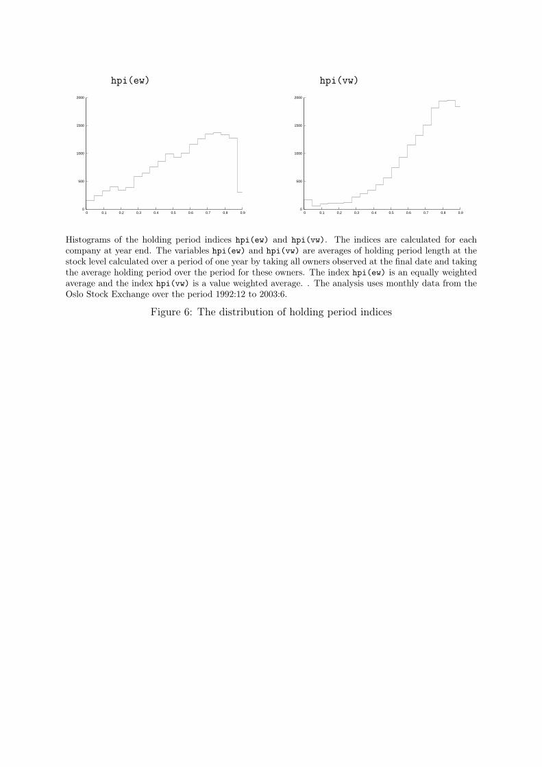
We calculate holding period indices for each firm in the sample. We do it for boththe equally weighted index hpi(ew) and the value weighted index hpi(vw). Figure 6shows the distribution of the two. Note the difference between the value weighted andequally weighted indices. That the value weighted index is more concentrated on thelonger period must be caused by the larger owners tending to stay longer. This suggestsa tendency that large owners have longer holding periods than small owners, a result wesaw for individual owners in the determinants of the hazard function.

4.2.2 What determines the holding period indices?

A simple way of evaluating how the holding period index varies with other firm char-acteristics is by stratifying the sample of firms based on the characteristic we want toinvestigate, and calculate averages for each group. Panel A of table 5 implements this for anumber of different firm characteristics: firm size, stock volatility, book-to-market (B/M)ratio, firm age, insider ownership and ownership concentration. The average holding pe-riods seem higher for the smallest and largest quartiles of the firms. A similar pattern istrue for volatility. The average holding period for value stocks (high B/M) seems to belonger than the average holding period for growth stocks. Firm age also seems important;the older the firm, the longer the average holding period. The last two variables, insiderownership and ownership concentration, show no obvious systematic patterns.

To test more formally the importance of the explanatory variables, we also run amultivariate regression for each of the two holding period indices. Panel B of table 5shows the results for this estimation. Old firms and value stocks tend to have ownerswith longer average holding periods than young firms and growth stocks. Surprisingly, wefind a negative coefficient on the firm size (though only significant for the equally weightedindex). Thus, we find weak evidence that larger firms have shorter duration ownershipthan smaller firms. This finding is at odds with the evidence in Atkins and Dyl (1997) aswell as with several suggested explanations for the opposite result that large firms shouldhave long duration owners than smaller firms (including less risk, reduced divergenceof investors’ expectations, and less need for portfolio re-balancing due to more stablereturn distribution parameters). The two variables thought to be related to asymmetricinformation, stock volatility and insider ownership, do not seem to explain averages ofholding periods for firms’ owners. Finally, the size of the largest owner is important; thelarger this owner, the longer the average holding period.

14

4.2.3 The relation between holding period index and other liquidity mea-sures

To investigate the relationship between liquidity measures and holding period, we look atthe covariability between these measures, and compare the properties of liquidity, suchas the liquidity’s determinants, to similar estimations for holding period indices.

We consider three different measures of liquidity: turnover, relative spread, and amor-tized spread. The turnover and relative spread are standard measures, and will not bediscussed further. The amortized spread is particularly interesting for our purposes, asit attempts to measure an expected cost of trading equity that takes into account theholding period of a position. As such it can be viewed as an attempt to make tradingcosts across stocks comparable by looking at expected costs over a defined time interval,such as a year. The amortized spread measure was introduced in Chalmers and Kadlec(1998), and is roughly equal to the bid/ask spread multiplied by turnover.19

Panel A in table 6 shows stratified averages of holding period indices. We see thatstocks with low turnover have longer holding period indices and that holding period isincreasing in the spread. These observations are confirmed by the correlation coefficientsin panel B of the table. All the coefficients have the expected signs. Note that in the cross-section, the correlation between turnover and the holding period indices is only around−0.5. This shows that turnover is an imperfect measure of holding period. Interestingly,the amortized spread has a very low correlation with the holding period indices. However,when we look at the quartiles of hpi there seems to be some systematic covariationbetween hpi and amortized spread.

To further investigate the links between the holding period indices and the liquiditymeasures we analyze the determinants of turnover and spreads in the same way as we didfor the holding period indices. The results from this analysis are presented in tables 7and 8, and should be compared to similar regressions for holding periods reported intable 5. As the tables show, the liquidity variables seem to have similar determinants as

19Chalmers and Kadlec (1998) used trading data to calculate the amortized spread for date T as

AST =∑T

t=1 |Pt −Mt|Vt

PT × SharesOutT

where AST is the amortized spread, Pt is a transaction price, Mt a midpoint price, Vt a trade quantityand SharesOut is the number of shares outstanding. Observation T is the last observation of the day.Since we do not have transaction data, only closing data and volume, we approximate the daily amortizedspread as

AS ≈ PT −MT

PT

∑t Vt

SharesOutT≈ Relative bid/ask spread× Turnover

Multiplying this by 252 gives a daily estimate of the annualized amortized spread. We use averages ofthis measure over a time period in most of our analysis.

15

the holding period indices; firm size, B/M ratio, and the size of the largest owner are allsignificant determinants of both turnover and spread.

We also show, in table 9, results from adding liquidity variables to the series of ex-planatory variables used in the regressions presented in panel B of table 5. The liquidityvariables are clearly significant determinants of the holding period indices, but most ofthe other variables are still significant.

5 The role of holding period for asset pricing

In this section we investigate the links between liquidity, holding period and asset returns.As was discussed briefly in the literature section, there are different possible reasons forholding periods to be linked to asset prices.

Amihud and Mendelson (1986) formalize the idea of a positive relationship betweenexpected returns net of trading costs and the holding period. Two propositions are derivedfrom their model. Proposition 1 states the spread-holding period relationship tested insubsection 3.3; assets with higher spreads should be allocated to portfolios with the sameor longer expected holding periods. Proposition 2 states that observed asset returnsshould be an increasing and concave function of the relative spread. Jointly these twopropositions imply that observed asset returns must also be an increasing and concavefunction of the expected holding period.20 This relationship between holding periodand asset returns is investigated by Datar et al. (1998), who find support for the jointproposition in Amihud and Mendelson (1986). However, they use turnover as a proxy forholding period, and as we have shown the correspondence between holding period andturnover is less than perfect.21

Yan and Zhang (2008) provide an alternative explanation for a link between holdingperiod and asset prices. Their empirical analysis suggest that short-term institutionsare better informed and exploit their informational advantage by active trading. Theseresults suggest that there might be returns differences between the portfolios of long andshort term investors due to differences in information.

In this section we ask whether asset prices in the cross section is related to holdingperiod differences across stocks. In a sense our analysis is exploratory, we simply ask towhat extent holding periods, as opposed to liquidity, matters for asset prices.

20Suppose that assets held by investors with a long expected holding period have the same or lowerreturns than assets held by investors with a short expected investment horizon. From Proposition 1,the assets held by the long term investors must have the highest spread. But then Proposition 2 cannothold.

21The results in Datar et al. (1998) might instead be interpreted as supportive to Proposition 2 in theAmihud and Mendelson (1986) model with turnover as an alternative proxy for liquidity.

16

To investigate this, we perform various asset pricing investigations. First, we performa simple analysis of the cross-section of stock returns based on portfolio sorting. Allstocks are sorted into portfolios based on five criteria: turnover, relative bid/ask spread,amortized spread, and the two holding period indices hpi(ew) and hpi(vw). The port-folio sorts are performed at year end. We then calculate portfolio returns for the nextyear before rebalancing the portfolios. We then calculate the averages of the excess re-turns for these five portfolio sorts and look for a systematic variation in excess returns.Table 10 shows the results from this analysis. For the portfolios sorted on the holdingperiod indices, we find no clear pattern in excess returns. However, for all three liquiditymeasures we find a clear systematic variation: the better the liquidity of a portfolio, thelower its excess returns.

While the orderings in panel A in table 10 are indicative, they are not sufficient toconclude that the holding period measures do a worse job in the cross-section. They maymerely reflect differences in risk. We therefore need to embed the question in a formalasset pricing analysis. There are numerous ways this type of analysis can be performed.We first do a simple correction for the three factor Fama and French (1995) model, bycalculating returns in excess of the Fama French model. Averages of these excess returnsare reported in panel B of table 10. While these numbers are more noisy than the returnsin excess of the risk free rate, since the Fama French parameters are estimated, they stillgive the same impression as the results in panel A, the sorts using the holding periodindices have less clear relationships with (Fama French) excess returns than the morestandard liquidity measures.

As a different way of asking the same question, we ask whether we can use portfoliossorted by liquidity/holding period to construct a pricing factor that helps explain thecross-section of stock returns. The construction of this “liquidity factor” (LIQ) is done bya sort similar to the Carhart (1997) construction, where we at year-end sort the stocksbased on the relevant liquidity/holding period measure, and take the difference in returnsbetween the 30% top and 30% bottom stocks. This liquidity factor is then used as anexplanatory variable in a joint estimation of the system

E[r] = βλ

r = a + βf

where f is the vector of pricing factors, and λ (factor loadings) and β (betas) are jointlyestimated. This is a well known formulation, see Cochrane (2005) for elucidation of theprocedure. In our formulation, we use two elements in f . One is the standard use of amarket portfolio, where we use an equally weighted market portfolio for the Oslo StockExchange. The second is the constructed factor based on liquidity or holding period

17

(LIQ). For our purposes, the interesting question is whether different versions of the LIQfactor is priced in the cross-section, which is to test whether λ is significantly differentfrom zero in an estimation on a set of test assets. As argued by Cochrane (2005), oneshould use a set of test assets with a decent cross-sectional variation. We therefore usea set of size-sorted portfolios.22 Table 11 shows the complete results of the estimationwhere we apply the market factor and a LIQ factor constructed from relative spread toeight size-sorted portfolios.

We observe that both the market portfolio and the liquidity factor are significantdeterminants of the cross-section. The market risk premium is positive, as it should be.More importantly, for our purposes, is the fact that the liquidity risk premium is positiveand significant. The importance of the liquidity factor is confirmed by the estimated betasfor the size-portfolios on the liquidity factor. Many of these are significant. Hence, we findthat a liquidity factor constructed from relative spread helps to explain the cross-sectionof returns of size-based portfolios.

We then repeat this exercise for four alternative measures of liquidity: turnover,amortized spread, hpi(ew) and hpi(vw). The results are summarized in table 12. Forbrevity, we only report estimates of β for the liquidity factor, and estimates of the factorpremia λ. To facilitate comparison, we also include the estimation using the LIQ factorestimated using the relative spread.

For our purposes, the most interesting result in Table 12 is the fact that while theliquidity factors constructed from spread and amortized spread are very significant de-terminants of the cross-section, the factors constructed from holding periods are not sig-nificant. This investigation reinforces our earlier finding that the holding period indicesdo a worse job than more standard liquidity measures in asset pricing applications.23

6 Conclusion

We use a data set of the complete holdings of all investors in a stock market to lookat expected holding periods for individual investors. We show how these decisions ofindividual investors sum up to a measure of average holding period at the stock level,and investigate the links between stock liquidity, holding periods, and asset returns.

We make a number of important contributions to the literature. First, we characterize22Empirical evidence, in e.g. Næs et al. (2008), shows that firm size is a significant determinant of the

cross-section of Norwegian stock returns.23We have implemented various other asset pricing tests, such as a Fama and MacBeth (1973) for-

mulation and a direct estimation of the components of the discount factor m, without the additionalstructure of the factor premia. We have also included the standard Fama French factors SMB and HML inthe analysis. In all cases the holding period indices are less significant than the other liquidity measures,in particular the spread measures, although there are cases where neither of them are significant.

18

the distribution of holding periods using duration analysis. Using these methods weshow that the median holding period is only 0.75 years. However, due to a very skeweddistribution, the average holding period is close to 2 years. This number is also what wouldbe estimated from (median) turnover. We also show that what is driving these results isa pattern of time variation in the conditional probability of selling the equity position.There is a high probability of exit the first year, and then steadily declining probability ofexit once the stock has been held for a year. We also analyze the holding period decisionsof individual investors and show that liquidity is an important determinant of holdingperiods for individual investors. Controlling for various investor specific and firm specificvariables, we find that low liquidity (high bid/ask spread and/or low turnover) of a stockwhen the investor enters into a stock position, tends to result in a longer holding period.

A second contribution is related to the relationship between holding period andturnover. Current empirical literature on the links between holding periods and assetreturns has used the inverse of turnover at the stock level as a proxy for expected holdingperiods for the individual investors of the stock (Atkins and Dyl, 1997). Based on thefinding that the correlation coefficient between turnover and holding period indices con-structed from data on actual holding periods lies around −0.5, we argue that turnover isonly an imperfect measure of expected holding periods.

Our third contribution is to provide empirical evidence that the link between liquidityand asset prices is not explained by investors who want compensation for exogenoustrading costs. Amihud and Mendelson (1986) suggest that the link between transactioncosts (spreads) and returns works through investors’ selection of stocks based on theirexpected holding periods. If this is the case, we should see that the average holding periodin a stock is an important determinant of the cross section of stock returns. However,when we compare our measures of average holding period and more traditional measuresof liquidity, such as spread and turnover, as determinants of the cross-section of stockreturns, we find that the more traditional liquidity measures have much stronger links toasset returns.

While our results are still preliminary, there are some interesting avenues for furtherresearch. As discussed in the introduction, the Amihud and Mendelson model does notexplain why there is a spread, just that different spreads can be sustainable when investorsselect stocks with different spreads based on their expected holding periods. A morecomplete model would also incorporate the cause of liquidity (spread) differences. Atypical microstructure model would attribute these causes to information risk. We findthat liquidity strongly affects holding periods. At the same time, we find little evidenceof a link between holding periods and returns, and a strong link between returns andtraditional microstructure liquidity variables. A possible explanation for these results is

19

that the cause of the first effect is the Amihud and Mendelson intuition, investors reactingto spreads, while returns and microstructure liquidity are linked through the cause ofspread differences. Trying to disentangle these effects seems a promising direction to go.

20

ReferencesViral A Acharya and Lasse Heje Pedersen. As-

set pricing with liquidity risk. Journal of Fi-nancial Economics, 77:375–410, 2005.

Yakov Amihud and Yakov Mendelson. Assetpricing and the bid/ask spread. Journal ofFinancial Economics, 17:223–249, 1986.

Yakov Amihud, Haim Mendelson, andLasse Heje Pedersen. Liquidity and assetprices. Foundations and Trends in Finance,1(4):269–363, 2005.

Allen B Atkins and Edward A Dyl. Transac-tions costs and holding periods for commonstocks. Journal of Finance, 52(1):309–325,March 1997.

Brad M Barber and Terrence Odean. Trad-ing is hazardous to your wealth: The com-mon stock investment performance of indi-vidual investors. Journal of Finance, 55(2):773–806, April 2000.

Øyvind Bøhren and Bernt Arne Ødegaard.The ownership structure of Norwegian firms:Characteristics of an outlier. Research Re-port Nr 13/2000, Norwegian School of Man-agement, September 2000.

Øyvind Bøhren and Bernt Arne Ødegaard. Pat-terns of corporate ownership: Insights froma unique data set. Nordic Journal of PoliticalEconomy, pages 57–88, 2001.

Mark M Carhart. On persistence in mutualfund performance. Journal of Finance, 52(1):57–82, March 1997.

John M R Chalmers and Gregory B Kadlec.An empirical examination of the amortizedspread. Journal of Financial Economics, 48(2):159–188, May 1998.

John Cochrane. Asset Pricing. Princeton Uni-versity Press, revised edition, 2005.

George M Constantinides. Capital market equi-librium with transaction costs. Journal ofPolitical Economy, 94(4):842–862, August1986.

Vinay T Datar, Narayan Y Naik, and RobertRadcliffe. Liquidity and stock returns: Analternative test. Journal of Financial Mar-kets, 1:203–219, 1998.

Jorge D Dias and Miguel A Ferreira. Timingand holding periods for commmon stocks:A duration-based analysis. Working Paper,ECB and ISCTE Business School-Lisbon,February 2005.

B Espen Eckbo and David C Smith. The condi-tional performance of insider trades. Journalof Finance, 53:467–498, April 1998.

Eugene F Fama and Kenneth R French. Sizeand book-to-market factors in earnings andreturns. Journal of Finance, 50(1):131–56,March 1995.

Eugene F Fama and J MacBeth. Risk, returnand equilibrium, empirical tests. Journal ofPolitical Economy, 81:607–636, 1973.

M Getmansky, A Lo, and I Makarov. An econo-metric model of serial correlation and illiq-uidity in hedge fund returns. Journal of Fi-nancial Economics, 74:529–610, 2004.

Shing-yang Hu. Trading turnover and expectedstock returns: The trading frequency hy-pothesis and evidence from the Tokyo stockexchange. Working Paper, University ofChicago, January 1997.

Ming Huang. Liquidity shocks and equilibriumliquidity premia. Journal of Economic The-ory, 109:297–354, March 2003.

Nicholas M Kiefer. Economic duration dataand hazard functions. Journal of EconomicLiterature, XXVI:646–679, June 1988.

Petri J Kyrolainen and Jukka Perttunen. DoIndividual Investors Care About TransactionCosts? Bid-Ask Spreads and Holding Peri-ods for Common Stock. SSRN eLibrary, De-cember 2006.

Tony Lancaster. Econometric models for theduration of unemplyment. Econometrica, 47(4):939–56, July 1979.

21

Randi Næs, Johannes Skjeltorp, andBernt Arne Ødegaard. What factorsaffect the Oslo Stock Exchange? WorkingPaper, Norges Bank and Norwegian Schoolof Management BI, May 2008.

Stephen J Nickell. Estimating the probabilityof leaving unemployment. Econometrica, 47(5):1249–66, September 1979.

G J van den Berg. Duration models: Spec-ification, identification and multiple dura-tions. In James J Heckman and Edward

Leamer, editors, Handbook of Econometrics,volume 5 of Handbooks in Economics, chap-ter 55, pages 3381–3453. Elsevier, 2001.

D Vayanos. Transaction costs and asset prices:A dynamic equilibrium model. Review of Fi-nancial Studies, 11(1):1–58, 1998.

Xuemin (Sterling) Yan and Zhe Zhang. Insti-tutional investors and equity returns: Areshort term institutions better informed. Re-view of Financial Studies, 2008.

22

-

FirstDate

LastDate

? ?

-Investor A

-Investor B

-Investor C

Calendar time1992 2003

The figure illustrates some conceptual problems in our estimation of holding periods using monthlyobservations. In calendar time our sample starts in 1992:12 and ends in 2003:6. We illustrate the holdingperiods of 3 example investors, A, B and C. For investor A the holding period is contained within 1992–2003, and therefore estimated correctly. For investor B we correctly observe the initial date but as theinvestor keeps his stake until after the last date, all we know is that we observe the stake on the last date.The holding period of this owners is underestimated due to right censoring. For owner C we correctlyobserve the terminal date, but we do not observe the first date, only that this owner was present in thefirst date of the sample, in 1992:12. Hence the holding period is underestimated due to left censoring.

Figure 1: Illustrating the censoring problem

Survival function0.

000.

250.

500.

751.

00

0 2 4 6 8 10analysis time

Kaplan−Meier survival estimate

Hazard function

.1.2

.3.4

.5


Smoothed hazard estimate

Estimated survival and hazard functions using all investor-company holding periods at the OSE in theperiod. The figure on the left is the estimated survival function. The figure on the right is the estimatedhazard function. Analysis time in years. The analysis is based on 1,417,186 observations. The estimatesare corrected for right censoring. The estimation uses a Weibull probability function. The analysis isperformed using Stata9. The analysis uses monthly data from the Oslo Stock Exchange over the period1992:12 to 2003:6.

Figure 2: Estimated hazard and survival functions

Financial owners.2

.3.4

.5.6

.7



Foreign owners

.2.4

.6



Nonfinancial owners

0.2

.4.6

.8



Individual owners

.1.2

.3.4

.5



State owners

0.2

.4.6

.8



We show estimated hazard functions for separate estimations for the five owner types. The estimationuses a Weibull probability function. Financial owners: Mutual funds, banks and insurance companies.Foreign owners: Owners domiciled outside of Norway, both corporations and individuals. Nonfinancialowners: Industrial owners (corporations that are not financials). Individual owners: Private individu-als/families. State owners: Public owners, including public pension funds. The analysis is performedusing Stata9. The analysis uses monthly data from the Oslo Stock Exchange over the period 1992:12 to2003:6.

Figure 3: Hazard functions estimated split by owner type

0

20

40

60

80

100

120

140

160

0 2 4 6 8 10 12 14 16 18 20

The histogram shows the distribution of estimates of the average holding period of investors. Holdingperiod is estimated as one divided by annual turnover. The analysis uses monthly data from the OsloStock Exchange over the period 1992:12 to 2003:6.

Figure 4: Average holding periods estimated from turnover

-

time(months)

time t

−1−2−3−4−5−6−7−8−9−10−11−12. . .Owner 1: -

Owner 2: -

Owner 3: -

Owner 4: -

The figure illustrates our method for creating a holding period index. We illustrate four example owners,1–4. We look at all owners during the year, and calculate each owner’s holding period in fractions of theyear. For owner 1 the holding period is 1, for owner 2 it is 5/12, for owner 3 it is 7/12, and for owner 4it is 3/12. A holding period index is calculated at time t. We only use the owners present at time t, andcalculate the weighted average of holding periods for the individual owners as hpi = w11+w3

712 +w4

312 .

We use two different weights. The first is equal weights. The resulting index is denoted hpi(ew). Thesecond is value weights: each owner receive weights based on the fraction of the company that ownerholds at date t. The resulting index is denoted hpi(vw).

Figure 5: Illustrating the method for creating a holding period index

hpi(ew)

0

500

1000

1500

2000

0 0.1 0.2 0.3 0.4 0.5 0.6 0.7 0.8 0.9

hpi(vw)

0

500

1000

1500

2000

0 0.1 0.2 0.3 0.4 0.5 0.6 0.7 0.8 0.9

Histograms of the holding period indices hpi(ew) and hpi(vw). The indices are calculated for eachcompany at year end. The variables hpi(ew) and hpi(vw) are averages of holding period length at thestock level calculated over a period of one year by taking all owners observed at the final date and takingthe average holding period over the period for these owners. The index hpi(ew) is an equally weightedaverage and the index hpi(vw) is a value weighted average. . The analysis uses monthly data from theOslo Stock Exchange over the period 1992:12 to 2003:6.

Figure 6: The distribution of holding period indices

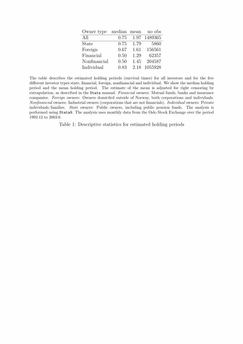
Owner type median mean no obsAll 0.75 1.97 1489365State 0.75 1.79 5860Foreign 0.67 1.61 156561Financial 0.50 1.29 62357Nonfinancial 0.50 1.45 204587Individual 0.83 2.18 1055928

The table describes the estimated holding periods (survival times) for all investors and for the fivedifferent investor types state, financial, foreign, nonfinancial and individual. We show the median holdingperiod and the mean holding period. The estimate of the mean is adjusted for right censoring byextrapolation, as described in the Stata manual. Financial owners: Mutual funds, banks and insurancecompanies. Foreign owners: Owners domiciled outside of Norway, both corporations and individuals.Nonfinancial owners: Industrial owners (corporations that are not financials). Individual owners: Privateindividuals/families. State owners: Public owners, including public pension funds. The analysis isperformed using Stata9. The analysis uses monthly data from the Oslo Stock Exchange over the period1992:12 to 2003:6.

Table 1: Descriptive statistics for estimated holding periods

Panel A: Investor-specific variables and liquidity

Variable Haz. Ratio pvalue Haz. Ratio pvalueln(Investment) 0.9773 (0.00) 0.9915 (0.00)Financial 1.1770 (0.00) 1.1579 (0.00)Foreign 0.9462 (0.00) 0.9362 (0.00)Nonfinancial 1.0851 (0.00) 1.0741 (0.00)Individual 0.7165 (0.00) 0.7114 (0.00)Bid Ask Spread 0.5221 (0.00)Turnover 1.1952 (0.00)n 1417186 1417186

Panel B: Investor-specific variables, firm-specific variables, and liquidity

Variable Haz. Ratio pvalueln(Investment) 0.9829 (0.00) 0.9887 (0.00)Financial 1.1916 (0.00) 1.2069 (0.00)Foreign 0.9932 (0.61) 0.9993 (0.95)Nonfinancial 1.1157 (0.00) 1.1356 (0.00)Individual 0.7551 (0.00) 0.7598 (0.00)ln(Volatility) 1.4317 (0.00) 1.2192 (0.00)ln(Firm Size) 1.0097 (0.00) 1.0411 (0.00)Bid Ask spread 0.0034 (0.00)Turnover 1.2288 (0.00)n 1038170

The tables show the results for two separate analyzes of contributions to the hazard function illustratedin figure 2. The contribution to the hazard function is estimated using a Weibull probability specification.The coefficients for each variable have the following interpretation: A number less than one in numericalvalue lowers the probability of exit, inducing a longer holding period. A number greater than one inducesa shorter holding period. In Panel A, the explanatory variables include investment size, owner type, andliquidity. In Panel B, we include volatility and firm size as explanatory variables in addition to investmentsize, owner type, and liquidity. Columns 2 and 3 show the results when we use the bid/ask spread asour measure of liquidity, while columns 4 and 5 show the results when we measure liquidity by turnover.Investment : The amount invested in that stock by the given owner, Financial : Dummy variable equalto one if the given owner is a financial corporation, Foreign: Dummy variable equal to one if the givenowner is foreign, Individual : Dummy variable equal to one if the given owner is an individual (family)owner, Nonfinancial : Dummy variable equal to one if the given owner is a nonfinancial corporation,Stock Volatility : Volatility of the stock’s returns, estimated using one year of returns, Firm Size: Thevalue of the company’s equity, Bid/Ask spread : Relative bid/ask spread (Pa − Pb)/Pt, averaged over ayear and Turnover : Number of shares traded in the stock during one year divided by number of sharesoutstanding. The analysis is performed using Stata9. The analysis uses monthly data from the OsloStock Exchange over the period 1992:12 to 2003:6.

Table 2: Determinants of the hazard function

Panel A: Determinants of the hazard function using spread as liquidity mea-sure

Investor type: Financial Foreign Nonfinancial Individual StateVariable Hazard p- Haz pval Haz pval Haz pval Haz pvalu

Ratio valueln(Investment) 1.0046 (0.09) 1.0511 (0.00) 1.0602 (0.00) 0.9494 (0.00) 1.0308 (0.00)ln(Volatility) 1.1922 (0.00) 1.2009 (0.00) 1.2027 (0.00) 1.3476 (0.00) 1.0069 (0.87)ln(Firm Size) 0.9567 (0.00) 1.0005 (0.86) 1.0170 (0.00) 1.0188 (0.00) 0.9429 (0.00)Rel B/A spread 0.0050 (0.00) 0.1134 (0.00) 0.0141 (0.00) 0.0259 (0.00) 0.0001 (0.00)n 48246 116750 154961 711225 4829

Panel B: Determinants of the hazard function using turnover as liquiditymeasure

Investor type: Financial Foreign Nonfinancial Individual StateVariable Haz. Ratio pvalue Haz pval Haz pval Haz pval Haz pvaluln(Investment) 1.0041 (0.13) 1.0530 (0.00) 1.0605 (0.00) 0.9568 (0.00) 1.0241 (0.00)ln(Volatility) 1.0595 (0.00) 1.1127 (0.00) 1.0816 (0.00) 1.1987 (0.00) 0.8294 (0.00)ln(Firm Size) 0.9884 (0.00) 1.0132 (0.00) 1.0441 (0.00) 1.0352 (0.00) 0.9990 (0.93)Turnover 1.1492 (0.00) 1.1363 (0.00) 1.1634 (0.00) 1.1593 (0.00) 1.2645 (0.00)n 48244 116711 154944 711176 4829

The tables show the results for five separate analyzes of contributions to the hazard functions illustratedin figure 3. The contribution to the hazard function is estimated using a Weibull probability specification.The coefficients for each variable have the following interpretation: A number less than one in numericalvalue lowers the probability of exit, inducing a longer holding period. A number greater than one inducesa shorter holding period. The explanatory variables are investment size, volatility, firm size and liquidity.In Panel A we use the relative spread as the liquidity measure. In panel B we use turnover as the liquiditymeasure. Investment : The amount invested in that stock by the given owner. Stock Volatility : Volatilityof the stock’s returns, estimated using one year of returns. Firm Size: The value of the company’sequity. Bid/Ask spread : Relative bid/ask spread (Pa−Pb)/Pt, averaged over a year. Turnover : Numberof shares traded in the stock during one year divided by number of shares outstanding. Financial owners:Mutual funds, banks and insurance companies. Foreign owners: Owners domiciled outside of Norway,both corporations and individuals. Nonfinancial owners: Industrial owners (corporations that are notfinancials). Individual owners: Private individuals/families. State owners: Public owners, includingpublic pension funds. The analysis is performed using Stata9. The analysis uses monthly data from theOslo Stock Exchange over the period 1992:12 to 2003:6.

Table 3: Determinants of hazard function estimated separately for each investor type

NYSE Nasdaq OSE1975-1989 1983-1991 1992-2003

Average 6.99 4.01 3.33Median 3.38 2.43 1.96

The table describes estimates of the average holding period of a stock’s investors using the methodof Atkins and Dyl (1997), where holding period is estimated as one divided by annual turnover, andcompare it to data for the US, from Atkins and Dyl (1997).

Table 4: Average holding periods estimated as in Atkins and Dyl (1997)

Panel A: Stratified quartiles

hpi(ew) hpi(vw)All 1 2 3 4 All 1 2 3 4

Firm Size 0.580 0.629 0.558 0.543 0.595 0.674 0.685 0.658 0.674 0.697Stock Volatility 0.570 0.630 0.548 0.522 0.579 0.682 0.714 0.667 0.664 0.684BM Ratio 0.577 0.463 0.565 0.599 0.651 0.685 0.640 0.690 0.695 0.706Firm listing age 0.579 0.477 0.554 0.610 0.642 0.672 0.616 0.657 0.680 0.717Primary insider fraction 0.577 0.580 0.590 0.588 0.562 0.672 0.671 0.670 0.672 0.672Largest owner 0.580 0.582 0.539 0.603 0.599 0.678 0.663 0.645 0.713 0.691

Panel B: Regression models

hpi(ew) hpi(vw)Variable coeff pvalue coeff pvalueconstant 0.767 (0.00) 0.548 (0.00)ln(Firm Size) -0.023 (0.00) -0.000 (0.98)Stock Volatility 0.579 (0.07) 0.414 (0.14)BM Ratio 0.059 (0.00) 0.036 (0.00)ln(Firm listing age) 0.102 (0.00) 0.038 (0.00)Primary insider fraction -0.122 (0.07) 0.056 (0.36)Largest owner 0.112 (0.00) 0.130 (0.00)n 1118 1118R2 0.30 0.11

The tables show how the holding period indices covary with firm characteristics. The top table (panel A)shows averages of holding period indices in stratified samples. For each line we group the stocks in thesample in four quartiles by the criterion listed on the left. We then calculate averages of holding periodindices for each of the four groups. The quartiles are sorted in increasing value. So, for example, in thefirst line quartile 1 is the group with the smallest companies, and quartile 4 contains the largest firms.The bottom table (panel B) shows results of two independent regressions showing how the holding periodindices listed at the top of each column are determined by the explanatory variables listed in the rows.The variables hpi(ew) and hpi(vw) are averages of holding period length at the stock level calculatedover a period of one year by taking all owners observed at the final date and taking the average holdingperiod over the period for these owners. The index hpi(ew) is an equally weighted average and the indexhpi(vw) is a value weighted average. . Firm Size: The value of the company’s equity. Stock Volatility :Volatility of the stock’s returns, estimated using one year of returns. B/M ratio: Book/Market Ratio.Listing age: Number of years on the stock exchange. Insider fraction: Fraction of the company held byinsiders. Largest owner : Fraction of the company owned by the firm’s largest owner. The analysis usesmonthly data from the Oslo Stock Exchange over the period 1992:12 to 2003:6.

Table 5: Determinants of holding period indices

Panel A: Stratified quartiles

hpi(ew) hpi(vw)All 1 2 3 4 All 1 2 3 4

Annual Turnover 0.579 0.723 0.636 0.552 0.426 0.674 0.793 0.737 0.666 0.515Annual Avg Rel BA Spread 0.576 0.515 0.550 0.573 0.690 0.671 0.642 0.649 0.672 0.735Annual Amortized Spread 0.576 0.647 0.562 0.534 0.559 0.673 0.727 0.671 0.648 0.643

Panel B: Correlations between liquidity and holding periods

Correlation Rank Correlationhpi(vw) hpi(ew) hpi(vw) hpi(ew)

Annual Turnover -0.509 -0.511 -0.478 -0.430Annual Avg Rel BA Spread 0.207 0.380 0.185 0.268Amortized Spread -0.079 -0.010 -0.118 -0.068

The table in Panel A splits the sample into four quartiles based on the two liquidity measures andshows how the holding period indices vary. The table in Panel B shows Pearson’s correlation coefficientsand Kendall’s rank correlation coefficients between holding period indices and liquidity measures. Thevariables hpi(ew) and hpi(vw) are averages of holding period length at the stock level calculated overa period of one year by taking all owners observed at the final date and taking the average holdingperiod over the period for these owners. The index hpi(ew) is an equally weighted average and theindex hpi(vw) is a value weighted average. Turnover : Number of shares traded in the stock during oneyear divided by number of shares outstanding. Bid/Ask spread : Relative bid/ask spread (Pa − Pb)/Pt,averaged over a year. Amortized Spread : The Chalmers and Kadlec (1998) definition of amortized spread,estimate of the annual cost of trading the stock. The analysis uses monthly data from the Oslo StockExchange over the period 1992:12 to 2003:6.

Table 6: The link between holding period indices and liquidity

Panel A: Turnover

Quartiles ofAll Annual Turnover

1 2 3 4Firm Size 301 136 222 515 334Stock Volatility 3.5 4.3 3.5 3.1 3.3BM Ratio 1.02 1.13 1.56 0.72 0.70Firm listing age 7.3 7.5 7.1 7.2 7.3Primary insider fraction 1.8 2.1 1.8 1.8 1.7Largest owner 26.9 32.8 28.9 23.1 23.2

Panel B: Relative bid/ask spread

Quartiles ofAll Annual Avg Rel BA Spread


Panel C: Amortized spread

Quartiles ofAll Annual Amortized Spread


The tables show how the liquidity variables covary with firm characteristics. Each table shows averagesof liquidity in stratified samples. For each line we group the stocks in the sample in four quartiles bythe criterion listed on the left. We then calculate averages of turnover, bid/ask spread and amortizedspread for each of the four groups. The quartiles are sorted in increasing value. So for example inthe first line quartile 1 is the group with the smallest companies, and quartile 4 contains the largestfirms. Turnover : Number of shares traded in the stock during one year divided by number of sharesoutstanding. Bid/Ask spread : Relative bid/ask spread (Pa − Pb)/Pt, averaged over a year. Firm Size:The value of the company’s equity. Stock Volatility : Volatility of the stock’s returns, estimated usingone year of returns. B/M ratio: Book/Market Ratio. Insider fraction: Fraction of the company held byinsiders. Listing age: Number of years on the stock exchange. Largest owner : Fraction of the companyowned by the firm’s largest owner. The analysis uses monthly data from the Oslo Stock Exchange overthe period 1992:12 to 2003:6.

Table 7: Determinants of liquidity measures - stratified quartiles

Annual Turnover Annual Avg Rel BA Spread Amortized SpreadVariable coeff pvalue coeff pvalue coeff pvalueconstant -0.166 (0.51) 0.200 (0.00) 0.032 (0.00)ln(Firm Size) 0.052 (0.00) -0.009 (0.00) -0.001 (0.00)Stock Volatility -0.259 (0.72) 0.530 (0.00) 0.056 (0.00)BM Ratio -0.115 (0.00) -0.001 (0.01) 0.000 (0.49)ln(Firm listing age) 0.006 (0.69) 0.003 (0.00) -0.000 (0.00)Primary insider fraction 0.249 (0.23) 0.005 (0.42) 0.002 (0.20)Largest owner -0.869 (0.00) 0.024 (0.00) -0.003 (0.00)n 1639 1639 1639R2 0.11 0.63 0.44

The table shows results of three independent regressions demonstrating how the liquidity variables listedat the top of each column are determined by the explanatory variables listed in the rows. Turnover :Number of shares traded in the stock during one year divided by number of shares outstanding. Bid/Askspread : Relative bid/ask spread (Pa − Pb)/Pt, averaged over a year. Amortized Spread : The Chalmersand Kadlec (1998) definition of amortized spread, estimate of the annual cost of trading the stock. FirmSize: The value of the company’s equity. Stock Volatility : Volatility of the stock’s returns, estimatedusing one year of returns. B/M ratio: Book/Market Ratio. Insider fraction: Fraction of the companyheld by insiders. Listing age: Number of years on the stock exchange. Largest owner : Fraction ofthe company owned by the firm’s largest owner. The analysis uses monthly data from the Oslo StockExchange over the period 1992:12 to 2003:6.

Table 8: Determinants of liquidity measures – regressions

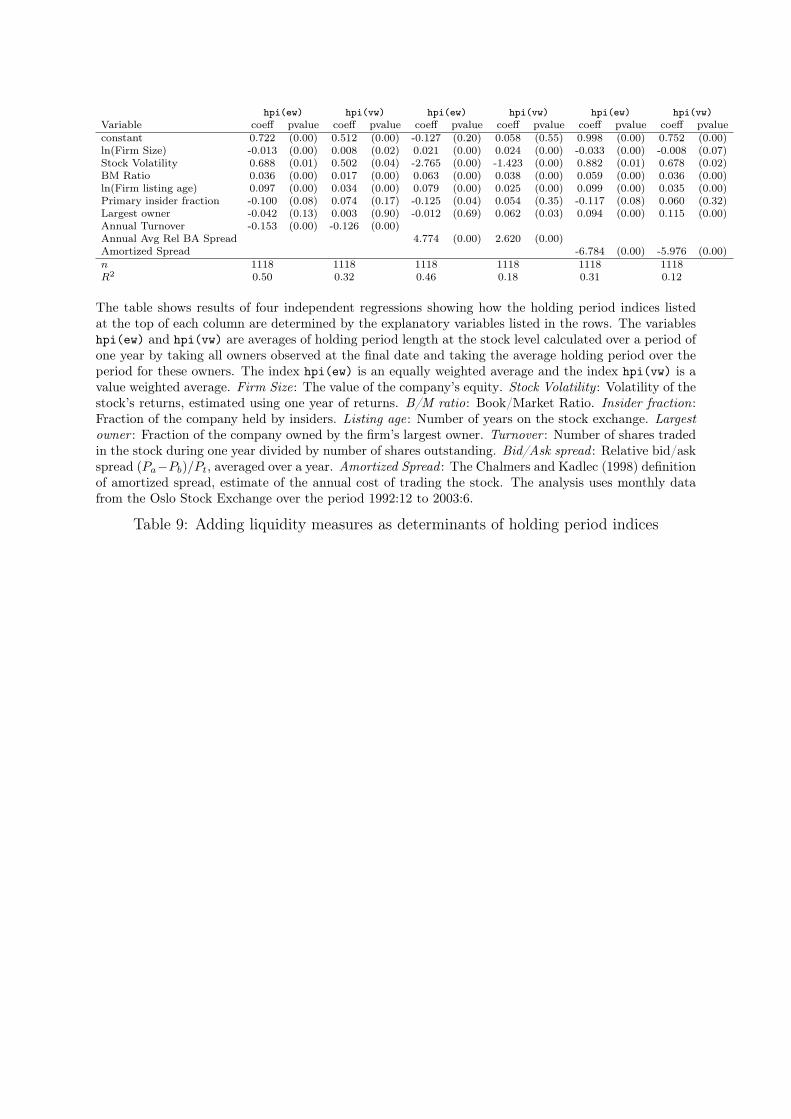
hpi(ew) hpi(vw) hpi(ew) hpi(vw) hpi(ew) hpi(vw)Variable coeff pvalue coeff pvalue coeff pvalue coeff pvalue coeff pvalue coeff pvalueconstant 0.722 (0.00) 0.512 (0.00) -0.127 (0.20) 0.058 (0.55) 0.998 (0.00) 0.752 (0.00)ln(Firm Size) -0.013 (0.00) 0.008 (0.02) 0.021 (0.00) 0.024 (0.00) -0.033 (0.00) -0.008 (0.07)Stock Volatility 0.688 (0.01) 0.502 (0.04) -2.765 (0.00) -1.423 (0.00) 0.882 (0.01) 0.678 (0.02)BM Ratio 0.036 (0.00) 0.017 (0.00) 0.063 (0.00) 0.038 (0.00) 0.059 (0.00) 0.036 (0.00)ln(Firm listing age) 0.097 (0.00) 0.034 (0.00) 0.079 (0.00) 0.025 (0.00) 0.099 (0.00) 0.035 (0.00)Primary insider fraction -0.100 (0.08) 0.074 (0.17) -0.125 (0.04) 0.054 (0.35) -0.117 (0.08) 0.060 (0.32)Largest owner -0.042 (0.13) 0.003 (0.90) -0.012 (0.69) 0.062 (0.03) 0.094 (0.00) 0.115 (0.00)Annual Turnover -0.153 (0.00) -0.126 (0.00)Annual Avg Rel BA Spread 4.774 (0.00) 2.620 (0.00)Amortized Spread -6.784 (0.00) -5.976 (0.00)n 1118 1118 1118 1118 1118 1118R2 0.50 0.32 0.46 0.18 0.31 0.12

The table shows results of four independent regressions showing how the holding period indices listedat the top of each column are determined by the explanatory variables listed in the rows. The variableshpi(ew) and hpi(vw) are averages of holding period length at the stock level calculated over a period ofone year by taking all owners observed at the final date and taking the average holding period over theperiod for these owners. The index hpi(ew) is an equally weighted average and the index hpi(vw) is avalue weighted average. Firm Size: The value of the company’s equity. Stock Volatility : Volatility of thestock’s returns, estimated using one year of returns. B/M ratio: Book/Market Ratio. Insider fraction:Fraction of the company held by insiders. Listing age: Number of years on the stock exchange. Largestowner : Fraction of the company owned by the firm’s largest owner. Turnover : Number of shares tradedin the stock during one year divided by number of shares outstanding. Bid/Ask spread : Relative bid/askspread (Pa−Pb)/Pt, averaged over a year. Amortized Spread : The Chalmers and Kadlec (1998) definitionof amortized spread, estimate of the annual cost of trading the stock. The analysis uses monthly datafrom the Oslo Stock Exchange over the period 1992:12 to 2003:6.

Table 9: Adding liquidity measures as determinants of holding period indices

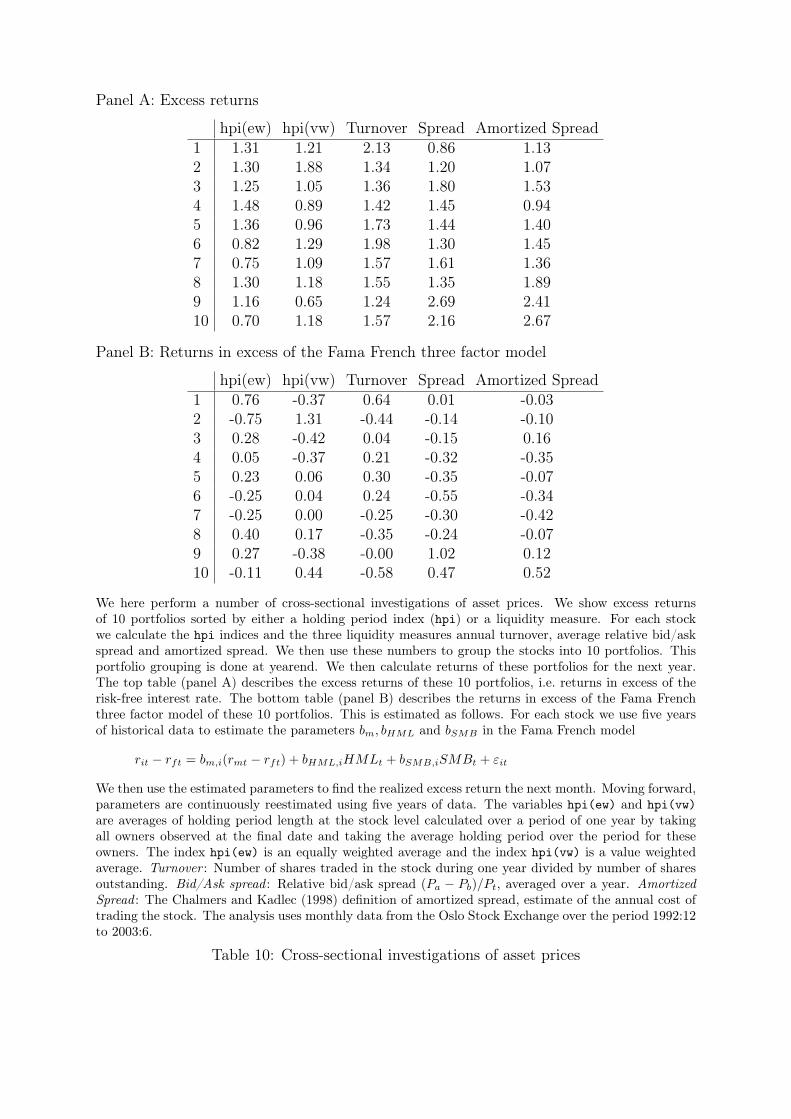
Panel A: Excess returns

hpi(ew) hpi(vw) Turnover Spread Amortized Spread1 1.31 1.21 2.13 0.86 1.132 1.30 1.88 1.34 1.20 1.073 1.25 1.05 1.36 1.80 1.534 1.48 0.89 1.42 1.45 0.945 1.36 0.96 1.73 1.44 1.406 0.82 1.29 1.98 1.30 1.457 0.75 1.09 1.57 1.61 1.368 1.30 1.18 1.55 1.35 1.899 1.16 0.65 1.24 2.69 2.4110 0.70 1.18 1.57 2.16 2.67

Panel B: Returns in excess of the Fama French three factor model

hpi(ew) hpi(vw) Turnover Spread Amortized Spread1 0.76 -0.37 0.64 0.01 -0.032 -0.75 1.31 -0.44 -0.14 -0.103 0.28 -0.42 0.04 -0.15 0.164 0.05 -0.37 0.21 -0.32 -0.355 0.23 0.06 0.30 -0.35 -0.076 -0.25 0.04 0.24 -0.55 -0.347 -0.25 0.00 -0.25 -0.30 -0.428 0.40 0.17 -0.35 -0.24 -0.079 0.27 -0.38 -0.00 1.02 0.1210 -0.11 0.44 -0.58 0.47 0.52

We here perform a number of cross-sectional investigations of asset prices. We show excess returnsof 10 portfolios sorted by either a holding period index (hpi) or a liquidity measure. For each stockwe calculate the hpi indices and the three liquidity measures annual turnover, average relative bid/askspread and amortized spread. We then use these numbers to group the stocks into 10 portfolios. Thisportfolio grouping is done at yearend. We then calculate returns of these portfolios for the next year.The top table (panel A) describes the excess returns of these 10 portfolios, i.e. returns in excess of therisk-free interest rate. The bottom table (panel B) describes the returns in excess of the Fama Frenchthree factor model of these 10 portfolios. This is estimated as follows. For each stock we use five yearsof historical data to estimate the parameters bm, bHML and bSMB in the Fama French model

rit − rft = bm,i(rmt − rft) + bHML,iHMLt + bSMB,iSMBt + εit

We then use the estimated parameters to find the realized excess return the next month. Moving forward,parameters are continuously reestimated using five years of data. The variables hpi(ew) and hpi(vw)are averages of holding period length at the stock level calculated over a period of one year by takingall owners observed at the final date and taking the average holding period over the period for theseowners. The index hpi(ew) is an equally weighted average and the index hpi(vw) is a value weightedaverage. Turnover : Number of shares traded in the stock during one year divided by number of sharesoutstanding. Bid/Ask spread : Relative bid/ask spread (Pa − Pb)/Pt, averaged over a year. AmortizedSpread : The Chalmers and Kadlec (1998) definition of amortized spread, estimate of the annual cost oftrading the stock. The analysis uses monthly data from the Oslo Stock Exchange over the period 1992:12to 2003:6.

Table 10: Cross-sectional investigations of asset prices

a rm spread1 0.0066 (0.25) 0.8557 (0.00) 0.5261 (0.00)

2 0.0024 (0.62) 0.7867 (0.00) 0.1386 (0.04)

3 0.0013 (0.79) 0.9873 (0.00) 0.0168 (0.84)

4 0.0030 (0.63) 1.1870 (0.00) 0.1553 (0.12)

5 0.0002 (0.96) 0.9364 (0.00) -0.0731 (0.26)

6 0.0001 (0.98) 1.0675 (0.00) -0.0953 (0.20)

7 -0.0045 (0.43) 0.9692 (0.00) -0.5160 (0.00)

8 -0.0037 (0.59) 0.9145 (0.00) -0.4365 (0.00)

λ1(rm) 0.0152 0.00λ2(spread) 0.0144 0.00

The table shows the result for estimating the system

E[r] = βλr = a + βf

where the relative spread has been used to generate the “liquidity factor” (LIQ). Bid/Ask spread : Relativebid/ask spread (Pa−Pb)/Pt, averaged over a year. The analysis uses monthly data from the Oslo StockExchange over the period 1994:1 to 2007:12.

Table 11: GMM estimation of factor portfolios

spread turnover am spread hpi(ew) hpi(vw)1 0.527 (0.00) -0.335 (0.07) 0.433 (0.00) 0.132 (0.02) 0.007 (0.90)2 0.139 (0.04) -0.061 (0.58) 0.083 (0.25) -0.003 (0.95) 0.002 (0.86)3 0.017 (0.84) 0.014 (0.91) -0.007 (0.93) -0.052 (0.19) 0.002 (0.84)4 0.156 (0.12) -0.092 (0.55) 0.164 (0.05) 0.027 (0.49) 0.004 (0.88)5 -0.073 (0.26) 0.056 (0.51) -0.074 (0.28) -0.061 (0.05) 0.001 (0.96)6 -0.095 (0.20) 0.060 (0.58) -0.056 (0.41) -0.068 (0.11) 0.001 (0.95)7 -0.516 (0.00) 0.331 (0.00) -0.400 (0.00) -0.189 (0.00) -0.003 (0.94)8 -0.436 (0.00) 0.255 (0.10) -0.328 (0.00) -0.166 (0.02) -0.003 (0.95)λ(m) 0.015 (0.00) 0.015 (0.00) 0.015 (0.00) 0.018 (0.00) 0.012 (0.70)λ(spread) 0.014 (0.00)λ(turnover) -0.025 (0.04)λ(am spread) 0.031 (0.00)λ(hpi(ew)) 0.044 (0.07)λ(hpi(vw)) 2.026 (0.91)

The table summarizes five different estimations of the system

E[r] = βλ

r = a + βf

The system is estimated using GMM. We use two factors, a market factor, erm, which is the excess returnon an equally weighted market index, and a liquidity factor LIQ, constructed from portfolios sorted byvarious liquidity factors. We only report the betas for the liquidity factor, not the alphas and betasagainst the market. The variables hpi(ew) and hpi(vw) are averages of holding period length at thestock level calculated over a period of one year by taking all owners observed at the final date and takingthe average holding period over the period for these owners. The index hpi(ew) is an equally weightedaverage and the index hpi(vw) is a value weighted average. Turnover : Number of shares traded in thestock during one year divided by number of shares outstanding. Bid/Ask spread : Relative bid/ask spread(Pa − Pb)/Pt, averaged over a year. Amortized Spread : The Chalmers and Kadlec (1998) definition ofamortized spread, estimate of the annual cost of trading the stock. The analysis uses monthly data fromthe Oslo Stock Exchange over the period 1994:1 to 2007:12.

Table 12: GMM estimation of factor portfolios

Documents

Liquidity and Asset Pricing: Evidence on the Role of ...finance.bi.no/~bernt/wps/holding_period/holding_period_paper_mar... · Liquidity and Asset Pricing: Evidence on the Role of