Linear Least Square s Problem

Math for CS Lecture 4 1

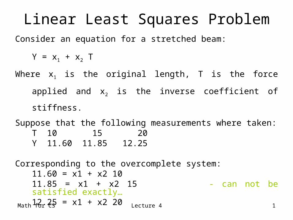
Linear Least Squares ProblemConsider an equation for a stretched beam:

Y = x1 + x2 T

Where x1 is the original length, T is the force applied and x2

is the inverse coefficient of stiffness.

Suppose that the following measurements where taken:T 10 15 20Y 11.60 11.85 12.25

Corresponding to the overcomplete system: 11.60 = x1 + x2 10

11.85 = x1 + x2 15 - can not be satisfied exactly… 12.25 = x1 + x2 20


Linear Least Squares Problem

Problem:

Given A(m x n), m≥n, b(m x 1) find x(n x 1) to minimize ||

Ax-b||2.

• If m > n, we have more equations than the number of

unknowns, there is generally no x satisfying Ax=b

exactly.

• This is an overcomplete system.


Linear Least Squares

There are three different algorithms for computing the least square minimum.

1. Normal Equations (Cheap, less Accurate).

2. QR decomposition.

3. SVD (expensive, more reliable).

The first algorithm in the fastest and the least accurate among the three. On the other hand SVD is the slowest and most accurate.


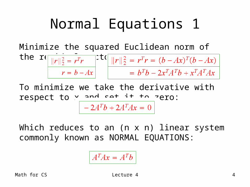
Minimize the squared Euclidean norm of the residual vector:

To minimize we take the derivative with respect to x and set it to zero:

Which reduces to an (n x n) linear system commonly known as NORMAL EQUATIONS:

Normal Equations 1


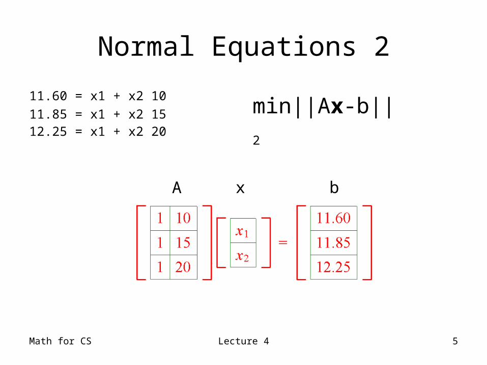
Normal Equations 2

11.60 = x1 + x2 10

11.85 = x1 + x2 1512.25 = x1 + x2 20

A x b

min||Ax-b||2


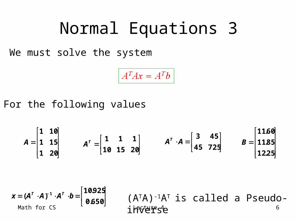
Normal Equations 3

201

151

101

A

72545

453AAT

201510

111TA

25.12

85.11

60.11

B

650.0

925.10)( 1 bAAAx TT

We must solve the system

For the following values

(ATA)-1AT is called a Pseudo-inverse


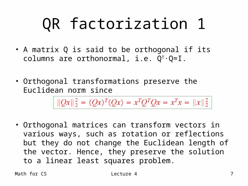
QR factorization 1

• A matrix Q is said to be orthogonal if its columns are orthonormal, i.e. QT·Q=I.

• Orthogonal transformations preserve the Euclidean norm since

• Orthogonal matrices can transform vectors in various ways, such as rotation or reflections but they do not change the Euclidean length of the vector. Hence, they preserve the solution to a linear least squares problem.


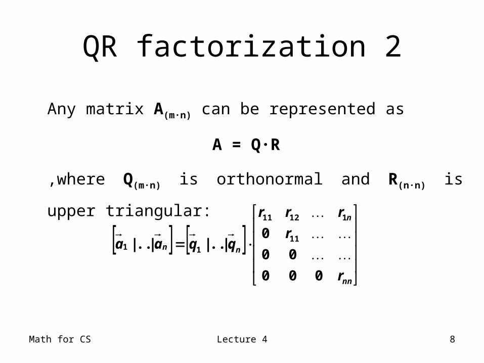
QR factorization 2

Any matrix A(m·n) can be represented as

A = Q·R

,where Q(m·n) is orthonormal and R(n·n) is upper triangular:

nn

n

nn

r

r

rrr

qqaa

000

00

0|...||...| 11

11211

11


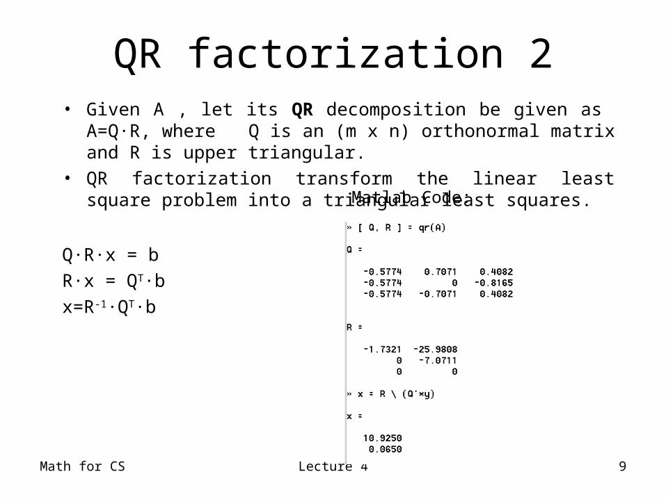
QR factorization 2• Given A , let its QR decomposition be given as A=Q·R, where

Q is an (m x n) orthonormal matrix and R is upper triangular. • QR factorization transform the linear least square problem into a

triangular least squares.

Q·R·x = b

R·x = QT·b

x=R-1·QT·b

Matlab Code:


Singular Value Decomposition

• Normal equations and QR decomposition only work for fully-ranked matrices (i.e. rank( A) = n). If A is rank-deficient, that there are infinite number of solutions to the least squares problems and we can use algorithms based on SVD's.

• Given the SVD:U(m x m) , V(n x n) are orthogonal

Σ is an (m x n) diagonal matrix (singular values of A)

The minimal solution corresponds to:


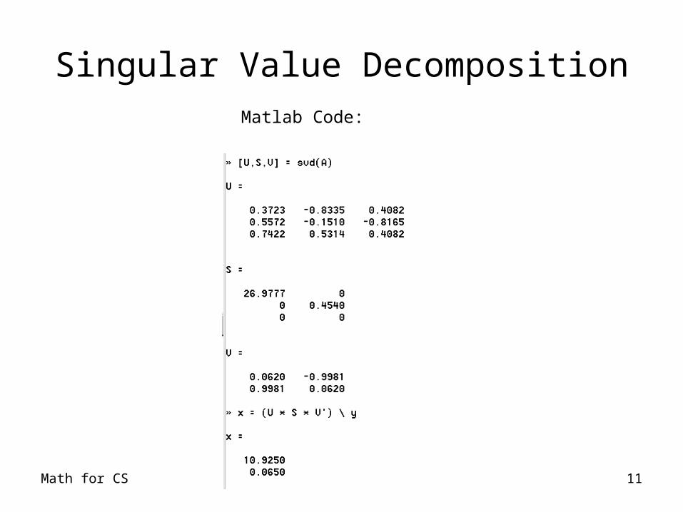
Singular Value DecompositionMatlab Code:


Linear algebra review - SVD

TT

TT

T

U ΣUAA

V V ΣAA

vuV ΣUA

Σ

IVV

IUU

ΣVU

AA

2

2

1

21

T

T

0 ),,...,,diag(

such that , ,exist there

,)rank( ,every for :Fact

p

i

Tiii

ip

pppnpm

nm p


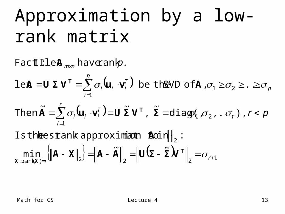
Approximation by a low-rank matrix

1222)(rank :

2

211

211

~~ min

:in ion toapproximat rank best theIs

),,...,,diag(~

,~

~

Then

... , of SVD thebe let

.rank have let :IIFact

rr

r

r

i

Tiii

p

p

i

Tiii

nm

r

pr

p

T

XX

T

T

VΣΣUAAXA

A

ΣV Σ UvuA

AvuV ΣUA

A


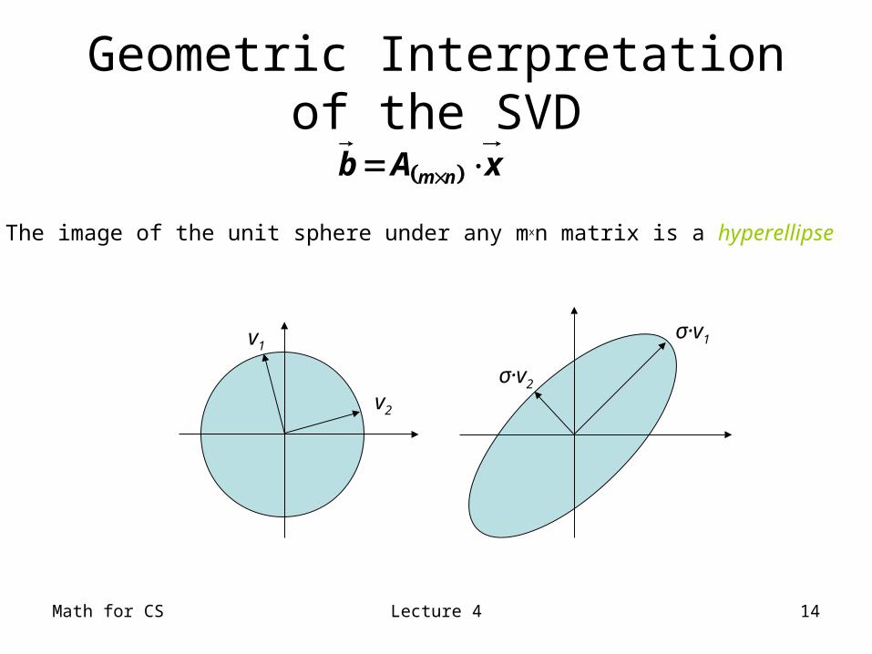
Geometric Interpretation of the SVD

xAb nm

The image of the unit sphere under any mxn matrix is a hyperellipse

v1

v2

σ·v2

σ·v1


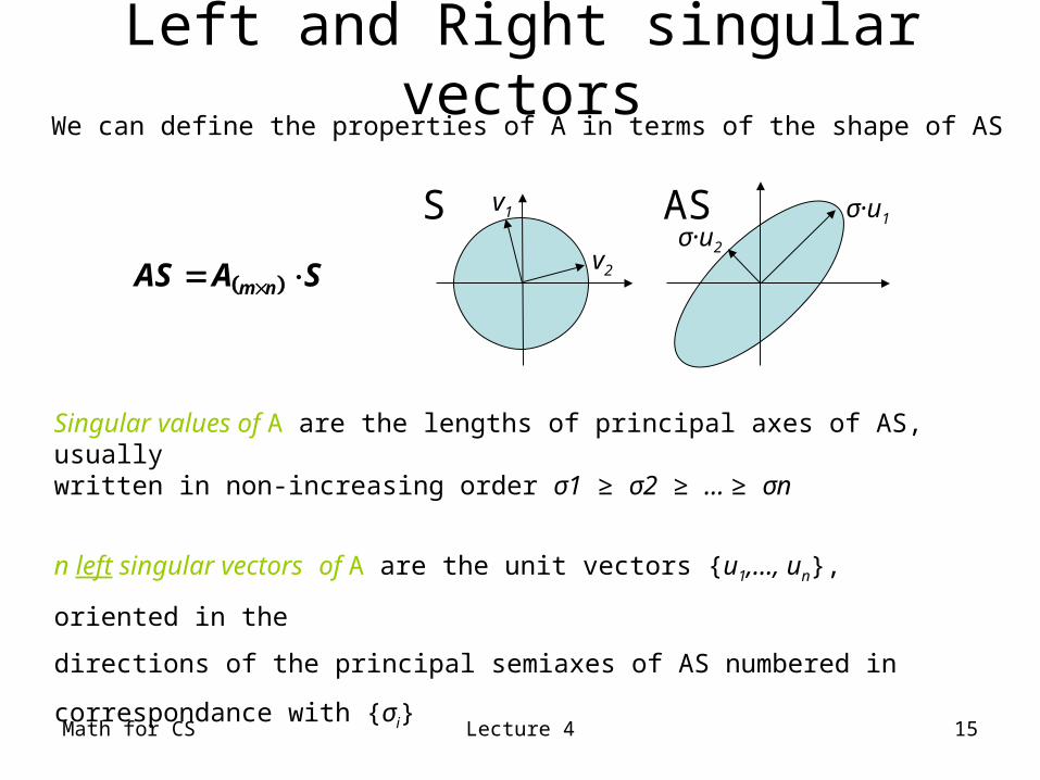
Left and Right singular vectors

SAAS nm

We can define the properties of A in terms of the shape of AS

v1

v2

σ·u2

σ·u1S AS

Singular values of A are the lengths of principal axes of AS, usuallywritten in non-increasing order σ1 ≥ σ2 ≥ … ≥ σn

n left singular vectors of A are the unit vectors {u1,…, un}, oriented in the

directions of the principal semiaxes of AS numbered in correspondance with {σi}

n right singular vectors of A are the unit vectors {v1,…, vn}, of S, which are the

preimages of the principal semiaxes of AS: Avi= σiui


Singular Value DecompositionAvi= σiui, 1 ≤ i ≤ n

),(

2

1

),(

21

),(

21

),(nnn

nm

n

nn

n

nm

uuuA

UAV

Matrices U,V are orthogonal and Σ is diagonal

- Singular Value decomposition*VUA


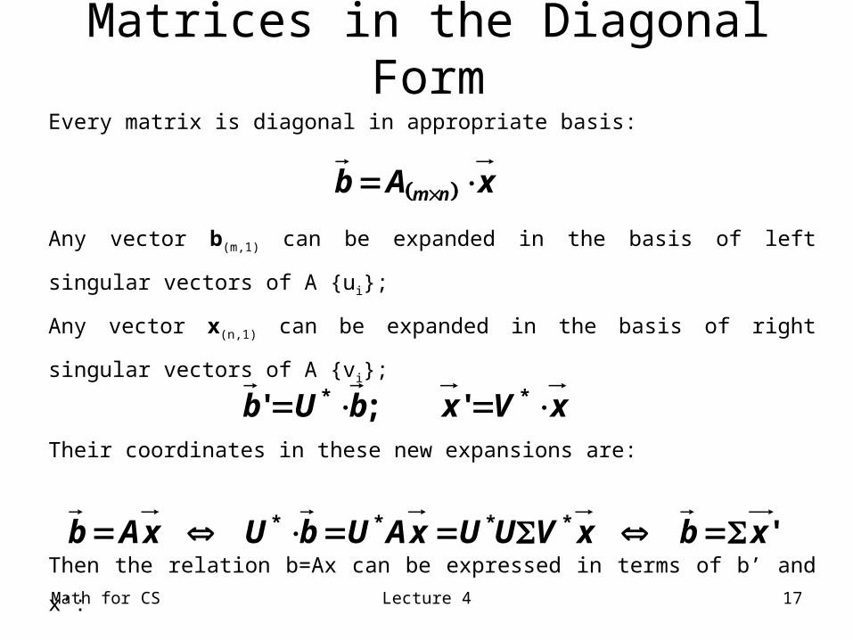
Matrices in the Diagonal FormEvery matrix is diagonal in appropriate basis:

Any vector b(m,1) can be expanded in the basis of left singular vectors of A {ui};

Any vector x(n,1) can be expanded in the basis of right singular vectors of A {vi};

Their coordinates in these new expansions are:

Then the relation b=Ax can be expressed in terms of b’ and x’:

xAb nm

xVxbUb ** ';'

'**** xbxVUUxAUbUxAb


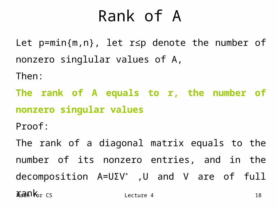
Rank of A

Let p=min{m,n}, let r≤p denote the number of nonzero

singlular values of A,

Then:

The rank of A equals to r, the number of nonzero

singular values

Proof:

The rank of a diagonal matrix equals to the number of its

nonzero entries, and in the decomposition A=UΣV* ,U and V

are of full rank


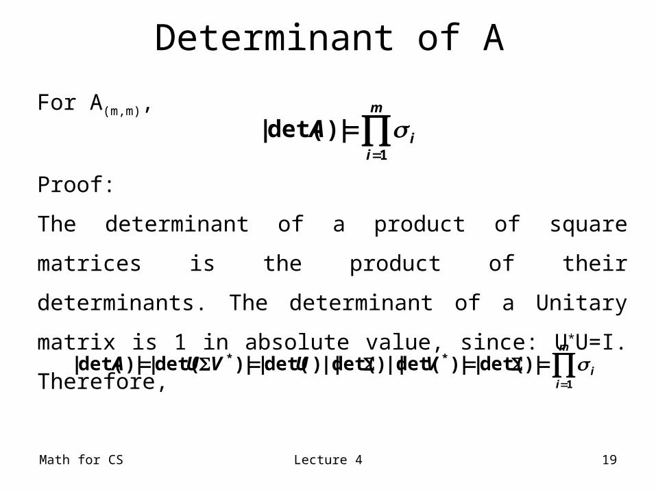
Determinant of A

For A(m,m),

Proof:

The determinant of a product of square matrices is the

product of their determinants. The determinant of a Unitary

matrix is 1 in absolute value, since: U*U=I. Therefore,

m

iiA

1

|)det(|

m

iiVUVUA

1

** |)det(||)det(||)det(||)det(||)det(||)det(|


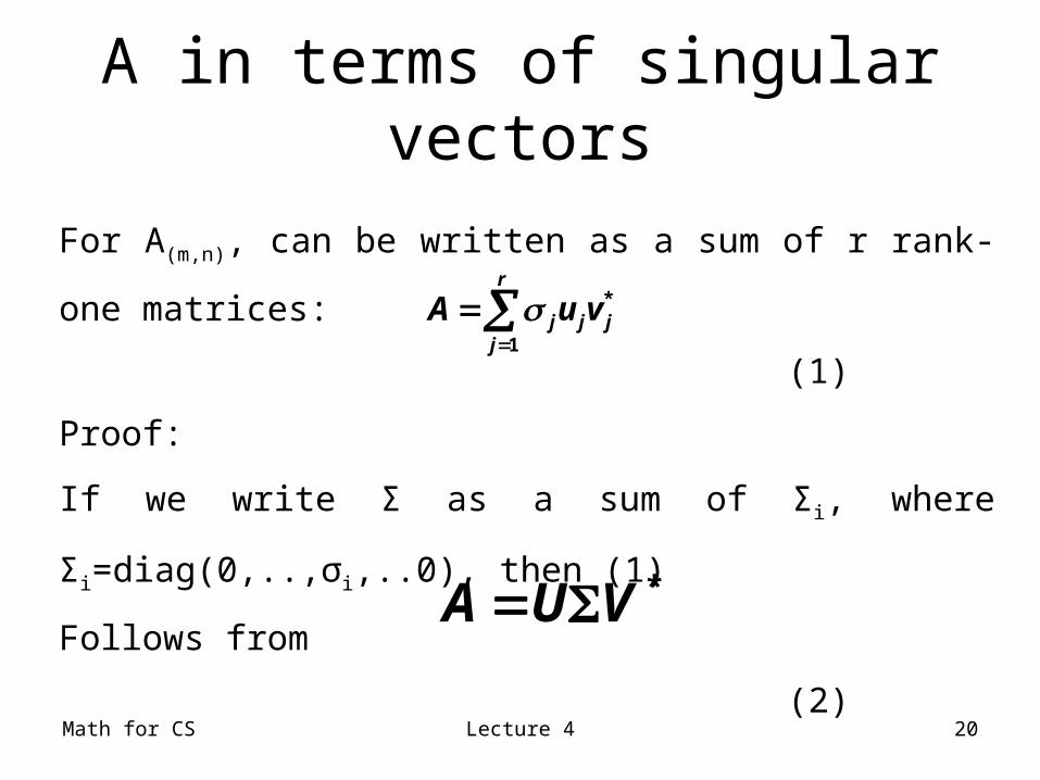
For A(m,n), can be written as a sum of r rank-one matrices:

(1)

Proof:

If we write Σ as a sum of Σi, where Σi=diag(0,..,σi,..0), then

(1)

Follows from

(2)

A in terms of singular vectors

r

jjjj vuA

1

*

*VUA


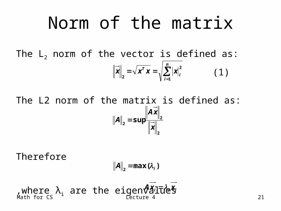
The L2 norm of the vector is defined as:

(1)

The L2 norm of the matrix is defined as:

Therefore

,where λi are the eigenvalues

Norm of the matrix

n

ii

T xxxx1

2

2

2

22

supx

xAA

)max(2 iA

iii xxA


For any ν with 0 ≤ ν ≤r, define

(1)

If ν=p=min{m,n}, define σv+1=0. Then

Matrix Approximation in SVD basis

v

jjjj vuA

1

*

12

)(

2inf

BAAA

Brank

CB nm

Documents

Linear Least Square s Problem