Linear Functional Equations and Convergence ofIterates

Axel Torshage

June 2012

Bachelor�s thesis 15 CreditsUmeå University

Supervisor - Yuriy Rogovchenko

Abstract

The subject of this work is functional equations with direction towards linearfunctional equations. The �rst part describes function sets where iterates of thefunctions converge to a �xed point. In the second part the convergence propertyis used to provide solutions to linear functional equations by de�ning solutions asin�nite sums. Furthermore, this work contains some transforms to linear form,examples of functions that belong to di¤erent classes and corresponding linearfunctional equations. We use Mathematica to generate solutions and solve itera-tively equations.

Contents

1 Introduction 31.1 Historical perspective . . . . . . . . . . . . . . . . . . . . . . . . . 31.2 Idea . . . . . . . . . . . . . . . . . . . . . . . . . . . . . . . . . . 61.3 Notation . . . . . . . . . . . . . . . . . . . . . . . . . . . . . . . . 7

1.3.1 Common notation . . . . . . . . . . . . . . . . . . . . . . . 71.3.2 Kuczma�s notation . . . . . . . . . . . . . . . . . . . . . . 71.3.3 New classes of functions . . . . . . . . . . . . . . . . . . . 8

2 Convergence of function iterates 92.1 Counterexample . . . . . . . . . . . . . . . . . . . . . . . . . . . . 112.2 Standard sets . . . . . . . . . . . . . . . . . . . . . . . . . . . . . 112.3 Simple extension . . . . . . . . . . . . . . . . . . . . . . . . . . . 122.4 Extension of the function�s class . . . . . . . . . . . . . . . . . . . 14

3 Linear Functional Equations 193.1 Homogenous linear functional equations . . . . . . . . . . . . . . . 19

3.1.1 Case (i) . . . . . . . . . . . . . . . . . . . . . . . . . . . . 213.1.2 Case (ii) . . . . . . . . . . . . . . . . . . . . . . . . . . . . 223.1.3 Case (iii) . . . . . . . . . . . . . . . . . . . . . . . . . . . 23

3.2 Criteria for Gn . . . . . . . . . . . . . . . . . . . . . . . . . . . . 243.3 Particular solution . . . . . . . . . . . . . . . . . . . . . . . . . . 26

3.3.1 Unique continuos solution . . . . . . . . . . . . . . . . . . 263.3.2 Arbitrary constant solution . . . . . . . . . . . . . . . . . 303.3.3 Arbitrary functions solution . . . . . . . . . . . . . . . . . 32

4 Transformations 354.1 Transformation to simpler linear form . . . . . . . . . . . . . . . . 354.2 Transformation of a general equation . . . . . . . . . . . . . . . . 36

1

5 Examples 385.1 Convergence . . . . . . . . . . . . . . . . . . . . . . . . . . . . . . 38

5.1.1 A function from R0� [I] . . . . . . . . . . . . . . . . . . . . 385.1.2 A function from S0� [I] . . . . . . . . . . . . . . . . . . . . 395.1.3 A function from P 0� [I] . . . . . . . . . . . . . . . . . . . . 415.1.4 A function from T 0� [I] . . . . . . . . . . . . . . . . . . . . 42

5.2 Solutions to linear functional equations . . . . . . . . . . . . . . . 445.2.1 A function from R0� [I] . . . . . . . . . . . . . . . . . . . . 445.2.2 A function from S0� [I] . . . . . . . . . . . . . . . . . . . . 455.2.3 A function from P 0� [I] . . . . . . . . . . . . . . . . . . . . 465.2.4 A function from T 0� [I] . . . . . . . . . . . . . . . . . . . . 46

6 Conclusions 49

7 Appendix 51

1. Introduction

In simple words, a functional equation is much like a regular algebraic equation,though instead of unknown elements in some set we are interested in �nding afunction satisfying our equation. A typical example of a functional equation is

' (x) + '�x2�= x;

where one has to �nd the function ' de�ned in some given interval. This equa-tion has a unique solution in [0; 1) and another one in (0;1) but no continuoussolutions in [0;1) : In Section 3 we will see that this example is linear as well.

1.1. Historical perspective

Even though functional equations were known long time before 17th century, ittook another two hundred years until mathematicians �rst tried to organize thenotations and theory. Grégoire de Saint-Vincent�s (1584-1667) work is a goodstarting point in the subject. He had noticed that the area under hyperbolicgraphs, for example, g (x) = x�1; can be described by a function with the proper-ties ' (x)+' (y) = ' (xy). This is the property possessed by logarithmic functionswhich is easily shown by modern calculus, but in that time Grégoire used a geo-metric argument to obtain a functional equation, which would ultimately have alogarithmic solution.However, the subject of functional equations at that time was rather undevel-

oped and we can date the real birth of the subject with the famous Augustin-LouisCauchy (1789-1857). Despite being most famous for his work in mathematicalanalysis, Cauchy has provided the basis of functional equations as well. TheCauchy equation

' (x+ y) = ' (x) + ' (y)

is one of the most important functional equations and is the �rst property of alinear functional often used in analysis and linear algebra. Cauchy also gave name

3

Figure 1.1: Grégoire de Saint-Vincent (1584-1667)

to the exponential counterpart ' (x+ y) = ' (x)' (y) and found the complete setof functions solving the d�Alambert equation

' (x+ y) + ' (x� y) = 2' (x)' (y) :

We introduce one more mathematician�s work. Charles Babbage (1791-1871)is known as a pioneer within computer science. Babbage�s work is closer to thedirection this paper has due to the fact that he studied various functional equationswith only one variable instead of the two used in the examples above. One familyof functional equations that Babbage introduced is of the type

G [x; ' (x) ; ' (a1 (x)) ; ::::; ' (an (x))] = 0;

where G; a1; ::::; an are known functions and ' is the unknown. This equation isof interest for us because by de�ning G in a certain way we can obtain a linearfunctional equation.

' (f (x))� g (x)' (x)� F (x) = 0:

We conclude this part by giving some further contribution to Babbage. Before we

Figure 1.2: Augustin-Louis Cauchy (1789-1857)

Figure 1.3: Charles Babbage (1791-1871)

4 2 2 4x

15

10

5

5

10

15

x

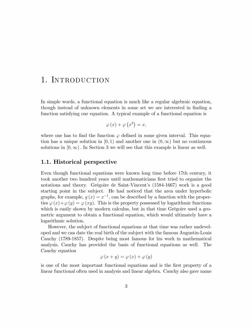
Figure 1.4: Solutions of the Babbage equation.

focus the linear functional equation, we shed some light on the Babbage equation.Though not linear, the following functional equation has some iterative valuesthat we may �nd interesting in this work:

' (' (x))� x = 0: (1.1)

Equation (1.1) is known as Babbage equation and involves an iteration of theunknown function ': The set of solutions to this equation is

' (x) = x; ' (x) = C � x; ' (x) =C

x; '

�C � x1 +Dx

�;

where C and D are arbitrary real constants. Here we plot four solutions to equa-tion (1.1), corresponding to the values C = 7 and D = 4:

1.2. Idea

The subject of functional equations has many similarities with that of di¤erentialequations. Just as in the case of di¤erential equations the appearance of thefunctional equation is crucial for the solution method. One di¤erence is thatfor real-valued functional equation one uses function iterates to �nd a solution.Convergence of these functions is an important property that allows to �nd asolution by the methods described in this paper. In this project, we discuss onlylinear functional equations.

1.3. Notation

We start by de�ning some notations that we will use in the sequel. Some of thesenotations might seem unrelated to the subject, but many of them describe quiteimportant properties of functional equations. Much of the notation used in thispaper coincides with the notation used in Marek Kuczma�s monograph [1], whichis the main source of information in this work.

1.3.1. Common notation

De�nition 1. We denote the most common interval as I; where I can be anyreal interval that �nite or in�nite. If nothing else is indicated, all functions arede�ned as f : I ! I; and x 2 I respectively. When a function is said to converge,it is understood that it converges in the interval I:

De�nition 2. Cn [I] denotes the n times di¤erentiable functions in the interval I:In this work we will at most times only demand that the functions are continuous,meaning that f 2 C0 [I].

1.3.2. Kuczma�s notation

De�nition 3. For a given f (x) and an interval I such that f : I ! I; we de�nethe n-th iterate as

f 0 (x) = x; fn+1 (x) = f (fn (x)) ; x 2 E; n 2 N [ f0g :

Not to be confused with exponentiation, which will be denoted (f (x))n and like-wise sin2 (x) = sin (sin (x)) ; not (sin (x))2 :

De�nition 4. A �xed point � 2 I corresponding to a certain function f is a pointsuch that f (�) = �:

There are certain sets that are of special interest, the intervals or sets whereour functions are de�ned. We will also de�ne some subsets of the set of functionsde�ned in I.

De�nition 5. The set Sn� [I] � Cn [I] is the set of functions such that

(f (x)� x) (� � x) > 0; x 6= �; (1.2)

and(f (x)� �) (� � x) < 0; x 6= �: (1.3)

De�nition 6. Rn� [I] denotes the subset of functions in Sn� [I] that are strictly

increasing.

De�nition 7. � [I] represents all functions ' : I ! �; where � is a given set (inthis work, � = R).

1.3.3. New classes of functions

De�nition 8. P n� [I] is the set of functions Pn� [I] � Cn [I] satisfying (1.2) and

(f (x) + x� 2�) (� � x) < 0; x 6= �: (1.4)

De�nition 9. T n� [I] � Cn [I] is the set of functions with the property (1.2) and

f (x)� ((k + 1) � � kx) < 0; 8x < �;(1.5)

kf (x)� ((k + 1) � � x) > 0; 8x > �;

where k is any constant larger then 0.

2. Convergence of function iterates

Convergence to a �xed point � is a valuable property of functions in this topic,many theorems will demand that some functions in the linear functional equationbehave in a certain manner. This chapter will discuss for which sets of functionswe can ensure this convergence property. First, we show that for the two setSn� [I] and R

n� [I] de�ned in Section 1.3 have convergence to a �xed point. Then,

we show that the same is true for the sets P n� [I] and Tn� [I]. There exist larger

sets containing converging functions, but these are not considered in this work.We will �rst prove an important lemma.

Lemma 10. Suppose that f : I ! I is a continuous function. Assume also that,for all � > 0; there exists a positive � < 1 such that jf (x)� x0j < � jx� x0j forx 2 In [x0 � �; x0 + �] ; where � might depend on �: Then limn!1 f

n (x) = x0:

Proof. We prove lemma by contradiction, suppose we have an x 2 I such that

f i�1 (x) 2 In [x0 � �; x0 + �] ; for all i � 1: (2.1)

Then the assumptions of the lemma ensure

jfn (x)� x0j < ���fn�1 (x)� x0�� < � � � ��fn�2 (x)� x0��

< � � � < �n jx� x0j : (2.2)

Then (2.2) yields

limn!1

jfn (x)� x0j < limn!1

�n jx� x0j = 0:

Hence, limn!1 fn (x) 2 [x0 � �; x0 + �] ; but this contradicts (2.1). Therefore, for

each x 2 I; there must exist an N � 1 such that

fN�1 (x) 2 [x0 � �; x0 + �]

9

If we can prove that

f : [x0 � �; x0 + �]! [x0 � �; x0 + �] ; (2.3)

thenfn�1 (x) 2 [x0 � �; x0 + �] ; n � N;

and letting �! 0; we have the convergence. Suppose the opposite to (2.3), f (x) 2In [x0 � �; x0 + �] for some x 2 [x0 � �; x0 + �] : If x = x0; by continuity of f andusing the fact that In [x0 � �; x0 + �] is an open set, there must exist a c > 0 de-pending on �; such that for all x 2 [x0 � c; x0 + c], f (x) 2 In [x0 � �; x0 + �] and bythe assumptions of the lemma, we can �nd an �2 > 0 such jf (x)� x0j < � jx� x0jfor some � < 1:Thus, jf (x)� x0j < jx� x0j and since x 2 [x0 � �; x0 + �], we havethat f (x) 2 [x0 � �; x0 + �] which contradicts the assumption. Thus we shouldhave x 6= x0; but we have shown that f (x) 2 In [x0 � �; x0 + �] is not possible ifx 6= x0: Thus, we have shown that (2.3) hold, hence we have proven convergence.

Lemma 11. Suppose that f is continuous in I and, for any � > 0; there existsan x0 2 I such that limn!1 f

n (x) = x0; for all x 2 [x0 � �; x0 + �] � I: Then,� = x0 is a �xed point of f and � is the only �xed point in [x0 � �; x0 + �] :

Proof. We use the fact that f is continuous to obtain

x0 = limn!1

fn (x) = f�limn!1

fn�1 (x)�= f (x0) ;

thus, x0 is a �xed point �. Suppose now we have a second �xed point �2 2[x0 � �; x0 + �] : Then, we have

�2 = f (�2) = f (f (�2)) = � � � fn (�2) :

Letting n!1, we havelimn!1

fn (�2) = �2 6= x0;

which contradicts the the assumptions of the proof. Thus, x0 is the only �xedpoint �:Note that Lemma 10 and Lemma 11 together yields a special case of Banach

�xed-point theorem.

2.1. Counterexample

One might get an idea that only (1.2) is enough to ensure convergence. Therefore,we show by a counterexample that there exists a function that satis�es (1.2) butfn (x) does not converge to �: Consider the function

f (x) = �2x:

For this function, we have the �xed point � = 0 as the only �xed point. We willshow now that this function satis�es (1.2):

(f (x)� x) (� � x) = (�3x)(�x) = 3x2 > 0 8x 6= 0:

On the other hand, fn(x) = (�2)n(x) ! �1 6= � as n ! 1; for any x 6= 0:This shows that we cannot ensure convergence by (1.2). However, adjusting thedemands by adding either of (1.3), (1.4) or (1.5), we can establish convergence.

2.2. Standard sets

We start by examining the sets de�ned by (1.2) and (1.3), namely Sn� [I] andRn� [I].

Since Rn� [I] is a subset of Sn� [I] ; it is enough to prove convergence for S

n� [I] to

ensure the same behavior for Rn� [I]. On the other hand, Sn� [I] is a subset of

even larger sets with the convergence property, but we will use more complicatedmethods in those proofs. The proof in this subsection is from [1, Theorem 0.4, p.21].

Theorem 12. Suppose that f 2 Sn� [I] : Then, limn!1 fn (x) = �: Furthermore,

the sequence fn (x) is strictly monotonic for x 6= �:

Proof. For x = �; the claim is trivial because if we have limn!1 fn (x) = �; �

is a �xed point by Lemma 11, so we suppose that x < �: The proof for the case� < x is similar. From (1.2) we have

(f (x)� x) (� � x) > 0:

Since x < �, we conclude that

f (x)� x > 0 () x < f (x) :

By (1.3), we have(f (x)� �) (� � x) < 0:

Hence,f (x)� � < 0 () f (x) < �:

Combining these results, we �nd that

x < f (x) < �:

Since f (x) < �; we can repeat this argument for f (x) n times to �nd that

fn (x) < fn+1 (x) ; n 2 N [ f0g :

So the sequence ff (x)gni=0 is monotonic (strictly increasing) for x < �: In thecase where � < x; it is strictly decreasing instead. To prove that this sequenceconverges to �; we simply need note

x� � < f (x)� � < 0:

It is easy to see thatjf (x)� �j < jx� �j :

For any x0 < �; � > 0 and any x in the interval [x0; � � �] � I; we can �nd apositive constant � < 1 such that

jf (x)� �j < � jx� �j :

Since f is de�ned in [x0; �] � I; by applying Lemma 10, we have the convergence.

2.3. Simple extension

We will show now the convergence for functions in the set P n� [I], but �rst we wantto show that P n� [I] is a larger set than S

n� [I] ; to be sure that (1.4) is a looser

condition than (1.3).

Proposition 13. Sn� [I] � P n� [I] :

Proof. Since both sets have the property (1.2), it is enough to prove that(1.3)=)(1.4) and thus, Sn� [I] has the property (1.4). By the assumption,

(f (x)� �) (� � x) < 0; x 6= �:

We simply subtract (� � x)2 on the left hand side of the inequality:

(f (x)� �) (� � x)� (� � x)2 < 0:

Therefore,(f (x) + x� 2�) (� � x) < 0;

and we are done.

Theorem 14. Assume that f satis�es (1.2) and (1.5) and I = [a; 2� � a] ; wherea < � might be in�nite. Then, f 2 P n� [I] and limn!1 f

n (x) = �; for all x:

Proof. To prove the theorem, we must show that f : I ! I and thus showingthat f 2 P n� [I] ; otherwise we cannot use these calculations. By (1.2) and (1.4),we have for x < �;

x < f (x) < 2� � x:Since x 2 I; x > a and we have

a < f (x) < 2� � a =) f (x) 2 I;

thus f 2 P n� [I] :For x = �; the claim is trivial because if we have limn!1 fn (x) =

�; � is a �xed point by Lemma 11. To show that limn!1 fn (x) = �; we therefore

suppose that x < � (for � < x the proof is similar). Condition (1.2) yields

(f (x) + x� 2�) (� � x) < 0;

and thus,f (x) > x: (2.4)

One the other hand, (1.4) provides the inequality

f (x) + x� 2� < 0() f (x)� � < � � x: (2.5)

Combining the inequalities (2.4) and (2.5), we obtain

x� � < f (x)� � < � � x: (2.6)

Suppose that f (x)� � � 0; then, by (2.6),

x� � < f (x)� � � 0;

and thus,jx� �j < jf (x)� �j :

Suppose now that f (x)� � > 0; then

0 < f (x)� � < � � x

andjf (x)� �j < j� � xj = jx� �j :

Therefore, in both cases, jf (x)� �j < j� � xj ; and, for any interval [x0; 2� � x0] �I; we have that for each � > 0 can �nd a positive � < 1 such that

jf (x)� �j < � j� � xj ; for all x 2 In [� � �; � + �] :

By Lemma 10, we proved the convergence.The fact that (1.2), (1.4) and I = [a; 2� � a] implies that f 2 P n� [I] is also

shown in the corollary to Lemma 16.

2.4. Extension of the function�s class

To enlarge the set for which we can establish convergence, we note that jf (x)� �j <j� � xj for x 6= � is not the only condition that provides functions that convergein I: It is, for example, enough to show that j� � fn (x)j < j� � xj for some n 2 Nand all x 6= �. This construction, however, is rather abstract and to check whethera function possesses this property is not something we will discuss in this paper.We will, however, discuss a special case that is more general and where it is rathereasy to verify if a function satis�es the assumptions and thus converges, by us-ing (1.5). We will, therefore, construct the set of functions T n� [I] and show thatfunctions in this set converge.

Proposition 15. P n� [I] � T n� [I] :

Proof. The construction of (1.5) says that f 2 T n� [I] provided that there existsa k > 0 such that condition (1.5) is satis�ed. Suppose f is a function verifying(1.5) for k = 1: Then, (1.5) states

f (x)� (2� � x) < 0 x < �;

andf (x)� (2� � x) > 0 x > �:

Multiplying both sides of the inequalities by (� � x) ; we obtain

(f (x) + x� 2�) (� � x) < 0 8x < �;(f (x) + x� 2�) (� � x) < 0 8x > �;

which is exactly (1.4), just divided in two cases. Thus, the functions f 2 P n� [I]belong also to T n� [I] and P

n� [I] � T n� [I] :

Lemma 16. Assume that f satis�es (1.2) and (1.5). Then f 2 T n� [I] if theinterval I is has the form I = [a; (k + 1) � � ka] ; for all a < �; where k is the sameas in the condition (1.5).

Proof. To prove f 2 T n� [I] we only have to show f : I ! I since the otherconditions we veri�ed due to assumption. Condition (1.5) gives us that for x < �

f (x)� ((k + 1) � � kx) < 0

and, since a � x;

f (x) < ((k + 1) � � kx) � ((k + 1) � � ka) : (2.7)

Condition (1.2) provides the lower bound as

a � x < f (x) :

Thus, f (x) 2 I for x < �: For x > � (1.5) yields

kf (x)� ((k + 1) � � x) > 0:

Since x � (k + 1) � � ka;

kf (x) > (k + 1) � � x � (k + 1) � � ((k + 1) � � ka) ; (2.8)

and we have the lower boundf (x) � a:

Assumption (1.2) provides the upper bound as

f (x) < x � (k + 1) � � ka;

so we have established that f is bounded in I for x 6= �; and thus, f (x) 2 I:Note that the fact that Lemma 16 tells nothing about the case when x = �

does not matter because if we can show convergence of T n� [I] ; we know that � isa �xed point by Lemma 10.

Corollary 17. f 2 P n� [I] is de�ned in In f�g if I = [a; 2� � a] ; for all a < �:

Proof. From Proposition 15, we know that P n� [I] is the set of functions in Tn� [I]

that satis�es (1.5) with k = 1: By Lemma 16, f is de�ned in I = [a; 2� � a] :

Theorem 18. Suppose that f 2 T n� [I] and I = [a; (a+ 1) � � kx] ; for somea < � that might be in�nite. Then, limn!1 f

n (x) = �; for all x:

Proof. From Lemma 16, we know that f is de�ned in I: We start by supposingthat x < �: Condition (1.5) yields

f (x)� ((k + 1) � � kx) < 0:

By rearranging terms, we have

f (x)� � < k� � kx = k (� � x) :

It follows from (1.2) that, for x < �; we have that x < f (x) ; so we can estimatef (x)� � below by

x� � < f (x)� � < k (� � x) : (2.9)

We will �nd now the corresponding bounds for � < x: Applying (1.5), we have

(kf (x)� ((k + 1) � � x)) (� � x) < 0:

Hence,kf (x)� ((k + 1) � � x) > 0;

or,� � xk

< f (x)� �:

Condition (1.2) yields that we have that f (x) < x; so we can estimate f (x) � �above by

� � xk

< f (x)� � < x� �: (2.10)

This concludes the proof of the �rst part of the theorem.We will show now that the boundaries get more tight for each iteration. We

start by showing that in (2.9), (2.10) the bounds di¤er in sign. This is obvioussince in (2.9) x� � < 0 and, for k > 0, k (� � x) > 0: The same is true for (2.10)since k�1 > 0: The method we use to prove the convergence is to show that these

boundaries shrink for each iteration, simply meaning that the lower estimate willincrease and the upper will decrease. Suppose that x < �; then we have theinequalities (2.9). Since the boundaries di¤er in sign we have two di¤erent cases,x� � < f (x)� � < 0 or 0 < f (x)� � < k (� � x) : There are actually three cases,there is also the case when f (x) � � = 0; but in that case we are sure that wehave convergence due to Lemma 11. Suppose that x � � < f (x) � � < 0. Then,f (x) < �; so we can apply another iteration and have by (2.9)

f (x)� � < f (f (x))� � < k (� � f (x)) :

Now, recalling that x < f (x) and k > 0; we get

x� � < f (x)� � < f (f (x))� � < k (� � f (x)) < k (� � x) :

Suppose now that0 < f (x)� � < k (� � x) ;

then f (x) > �; (2.10) yields

� � f (x)k

< f (f (x))� � < f (x)� �:

Applying (2.9) and using the fact that

f (x)� � < k (� � x)() (� � f (x)) k�1 > x� �;

we have

x� � < � � f (x)k

< f (f (x))� � < f (x)� � < k (� � x) : (2.11)

Thus, the boundaries shrink with each iteration when x < �: It remains to shownow the same for x < �: In that case, we have the inequalities (2.10). Onceagain, we can use the fact that the limits di¤er in sign to be sure that either0 < f (x) � � < x � � or (� � x) k�1 < f (x) � � < 0: For f (x) � � = 0;the convergence is trivial due to Lemma 11. We prove now that the boundariesshrink in both cases. Suppose that 0 < f (x)� � < x� �; then � < f (x) ; and wecan use (2.10),

f (x)� � > f (f (x))� � > � � f (x)k

:

Since f (x)� � < x� �; we can add the inequalities,

x� � > f (x)� � > f (f (x))� � > � � f (x)k

>� � xk:

Therefore, new boundaries are stricter. Suppose now that (� � x) k�1 < f (x) �� < 0; then f (x) < �; and we can use (2.9):

f (x)� � < f (f (x))� � < k (� � f (x)) :

But then, using (� � x) k�1 < f (x) � � and � � x < k (f (x)� �) ; or x � � >k (� � f (x)) ; we obtain,

� � xk

< f (x)� � < f (f (x))� � < k (� � f (x)) < x� �: (2.12)

Consequently, in both cases, the limits shrink under iteration. The � reasoning inthe two following cases are the same as that in Lemma 10 and are therefore leftout of this text. If we use (2.11) inductively for any x 2 [x0; �] � I; (2.11) yieldsthat for each � > 0 there exists a positive � < 1 such that

�n (� � x) < fn (x)� � < �nk (x� �) : (2.13)

Letting n ! 1; note that (2.13) states that fn (x) � � converges to 0 and thus,limn!1 f

n (x) = �: Likewise, for x 2 [�; (k + 1) � � kx0] � I; inequality (2.12)yields

�n�� � xk

�< fn (x)� � < �n (x� �) ;

and limn!1 fn (x) = �:for x 2 [x0; (k + 1) � � kx0] � I: Since x0 < � is any point

in I; we have proved convergence.

3. Linear Functional Equations

There are di¤erent types of functional equations, but from now on we discuss onlythe linear case.

De�nition 19. A functional equation is linear if it can be written as

' (f (x)) = g (x)' (x) + F (x) ; (3.1)

where g; F 2 � [I] ; f 2 T n� [I] ; g (x) 6= 0 in I;and ' is some unknown function in� [I] :

The work in this chapter are mostly based on [1, p. 46-66]. Even thoughmany results are similar, [1, p. 46-66] is focused on the case when f 2 Rn� [I] andeventually f 2 Sn� [I]. The contribution of this work in this chapter is to generalize[1, p. 46-66] to T n� [I] which is a more general set of functions In most cases weestablish almost the same results as in [1, p. 46-66].

3.1. Homogenous linear functional equations

De�nition 20. A homogenous linear functional equation is equation of the form

' (f (x)) = g (x)' (x) : (3.2)

To be able to provide solution to (3.1), we recall the idea of a solution toa linear di¤erential equation where one starts by �nding a general solution fora homogenous equation. Thereafter, we search for a particular solution: As thefollowing results show, some properties of linear functional equations are closethose of linear di¤erential equations.

Proposition 21. Suppose that '1 and '2 are solutions to equation (3.1). Then'3 = � ('1 � '2) where � 2 R; is a solution to the corresponding homogenouslinear functional equation (3.2).

19

Proof. Let '1 and '2 be solutions to equation (3.1). Then

� ('1 (f (x))� '2 (f (x))) = � (g (x)'1 (x) + F (x)� (g (x)'2 (x) + F (x))) :

That is,'3 (f (x)) = g (x)'3 (x) ;

and '3 solves the homogenous equation.

Proposition 22. Suppose that '1 and '2 are solutions to a homogenous linearfunctional equation (3.2), then '3 = �'1 + �'2 where �; � 2 R solves thathomogeneous equation.

Proof. The proof is immediate,

'3 (f (x)) = �'1 (f (x)) + �'2 (f (x)) =

g (x)�'1 (x) + g (x) �'2 (x) = g (x)'3 (x) ;

and thus '3 solves (3.2).For a linear functional equation (3.2), properties of the functions g and f are

very important.

De�nition 23. For a given linear functional equation, we de�ne Gn as

Gn (x) =n�1Yi=0

g�f i (x)

�; n 2 N; (3.3)

and, provided the limit exists in I; we de�ne G (x) by

G (x) = limn!1

Gn (x) :

The behavior of this function is important for the appearance of the sets ofsolutions. We will consider three di¤erent cases and show that the behavior ofsolutions is quite di¤erent. Case (i) : The limit of G (x) exists and is not 0 in I:Case (ii) : There exists some interval J � I such that G (x) = 0 in J and � 2 J:Finally, we have case (iii) which says simply that neither (i) or (ii) occurs. Thesecases will in the following part of this paper only be referred to as case (i) ; (ii)and (iii) ; due to their importance.

3.1.1. Case (i)

Theorem 24. Suppose we have homogenous linear functional equation with thecase (i) satis�ed, g; F 2 � [I] and f 2 T 0� [I] : Then, for each initial value � 2 �;there exists exactly one solution for each value ' (�) = �:

Proof. Since f : I ! I; we can use iterates to obtain, after p iterates,

'�fp+1 (x)

�= g (fp (x))' (fp (x)) : (3.4)

We will preform now the proof by induction, with the induction hypothesis

' (x) =' (fn (x))

Gn (x)n 2 N; (3.5)

and the basis n = 1: For n = 1; our claim is that

' (x) =' (f 1 (x))

G1 (x)=' (f (x))

g (x):

Since g (x) 6= 0; this is equivalent to (3.2), and thus is true. Suppose now that(3.5) holds for some n = p;

' (x) =' (fp (x))

Gp (x):

It follows from (3.4) that

' (fp+1 (x))

g (fp (x))= ' (fp (x)) :

Using the induction hypothesis and (3.4), we obtain

' (x) =' (fp (x))

Gp (x)=

' (fp+1 (x))

g (fp (x))Gp (x); (3.6)

which can be written as

' (x) =' (fp+1 (x))

Gp+1 (x):

Finally, the induction says that this is true for all n � 1: Since the limit of G (x)exists and f converges by Theorem 18, we can let n!1 to obtain

' (x) =' (�)

G (x):

For any value � 2 R; we �nd a unique solution as

' (x) =�

G (x):

Since G (x) is supposed to be continuous, so is ' (x) :We also note that g (�) mustbe equal to 1 because otherwise, G (�) would not converge to a nonzero value and(i) would not occur.

3.1.2. Case (ii)

An explicit solution is hard to �nd in this case. The reason is mainly becausethe functions in our set T 0� [I] are not necessarily strictly increasing. In case (ii) ;lack of this property makes it harder to �nd solutions. In Kuczma�s work [1]corresponding theorems are established for the functions from R0� [I] ; which is amuch more restrictive set. The mathematics of this will be left out here, but thedetails can be found in [1, pp. 49-50]. It is a result of the fact that, for functions inR0� [I] ; monotonicity property is very important for deducing the following: Everycontinuous function '0 (x) ; de�ned in some subset [f (x0) ; x0] or [f (x0) ; x0] of I;can be uniquely extended to J � I provided that '0 is a solution to (3.2) for x0:J is the part of I where x � � or � � x; respectively. This is not possible in ourcase, but we provide a useful result tailored to the functions from T 0� [I] :

Theorem 25. Suppose that Gn (x) converges uniformly to zero when n ! 1;in some interval J � I; where � 2 J: Then, for each continuous function '0that is a solution to the linear functional equation in some subinterval K =[c; k (� � c) + �] ; where c < �; '0 (x) can be continuously extended to ' (x) onthe entire interval I; and this extension is unique. Furthermore, ' (�) = 0:

Proof. To prove that ' (�) = 0; we recall that identity (3.5) is equivalent to

' (x)Gn (x) = ' (fn (x)) :

Let n!1 and suppose that x 2 J: Then we have, due to Theorem 18,

' (x) � 0 = ' (�) = 0:

To prove the possible extension to I; observe that Lemma 16 ensures that f :K ! K: Since by Theorem 18 f converges to �; we conclude that, for each x 2 I;there exists an N 2 N such that fN (x) 2 K: Equation (3.5) yields

' (x) =' (fn (x))

Gn (x)='0 (f

n (x))

Gn (x); n � N:

This is a well de�ned function since '0 (x) is known, and it is unique since f :K ! K. Continuity follows easily from the fact that both f and g are continuosfunctions applied a �nite number of times to obtain ' (x).The fact that f 2 T 0� [I] makes it hard to �nd solutions to nonhomogeneous

equations if we meet the case (ii) ; something we will experience in the followingsubsection as well.

3.1.3. Case (iii)

This condition on Gn is very restrictive, even though it might not seem like it.

Theorem 26. Assume that Gn (x) neither converges to a non-zero value, norit converges uniformly to zero in a interval J � I: Then, ' (x) = 0 is the onlysolution of (3.2) in I:

Proof. Suppose that ' (x) 6= 0 for some x 2 I; then (3.5) yields

Gn (x) =' (fn (x))

' (x):

Since ' [fn (x)] does not diverge and ' (x) 6= 0; we can let n ! 1 to obtain

limn!1

Gn (x) =' (�)

' (x):

If ' (�) 6= 0; we have case (i) since G (x) would exist and be nonzero. Therefore,we must have that ' (�) = 0: We have an interval � =2 J � I such that ' (x) 6= 0;otherwise case (ii) would occur. Since ' (x) 6= 0 and ' (x) is continuous, thereexists a constant C such that

j' (x)j > C > 0; for x 2 J:

Furthermore, for each given � > 0; there exists a c < � such that

j' (x)j < C�; for x 2 [c; (k + 1) � � kc] :

Due to Theorem 18 and Lemma 16, we can also �nd an N such that

fn (x) 2 [c; (k + 1) � � kc] ; for x 2 J and n � N:

But then, jfn (x)j < C�; and (3.5) gives us

jGnj =j' (fn (x))jj' (x)j < �; for x 2 J and n � N:

Thus, we have uniform convergence to zero in the interval [c; (k + 1) � � kc] andthe case (ii) : Therefore, the only possible solution for the homogenous equationis the trivial solution.

3.2. Criteria for Gn

Since the behavior of Gn is important, we will �nd now some criteria that help todetermine which of the cases occurs.

Theorem 27. Suppose that jg (�)j < 1; g 2 � [I] ; and f 2 T 0� [I] : Then, Gn (x)converges uniformly to zero in some interval J � I as n!1:

Proof. Since jg (�)j < 1 and g (x) is continuos, there exists a � > 0 such that,for x 2 J; J = [� � �; � + k�] ; we have that jg (x)j < C < 1 for some C: De�nec = � � �; then we have J = [c; (k + 1) � � kc] : Since f converges to �; accordingto Theorem 18, f : J ! J and, due to Lemma 16, there exists an N such that

fn (x) 2 [c; (k + 1) � � kc] ; for x 2 J and n � N:

We evaluate now Gn in J;

jGn (x)j =�����n�1Yi=0

g�f i (x)

������ =�����N�1Yi=0

g�f i (x)

� n�1Yi=N

g�f i (x)

������<

�����N�1Yi=0

g�f i (x)

������Cn�N :The �rst product is bounded since it is a �nite product of �nite elements and theother approaches zero as n!1; so case (ii) will occur.A similar proof is carried out for jg (�)j � 1:

Theorem 28. Suppose that there exists an interval J = [c; (k + 1) � � kc] suchthat jg (x)j � 1; g (�) 6= 1; g (x) 2 � [I] and f 2 T 0� [I] : Then, the case (iii) occurs.

Proof. We know that jg (�)j � 1 in J: Furthermore, according to Theorem 18, fconverges to � and, by Lemma 16, f : J ! J: Therefore, there exists an N suchthat

fn (x) 2 [c; (k + 1) � � kc] ; n � N:We evaluate Gn (x) to show that (ii) can not occur,

jGn (x)j =�����n�1Yi=0

g�f i (x)

������ =�����N�1Yi=0

g�f i (x)

�����������n�1Yi=N

g�f i (x)

������������N�1Yi=0

g�f i (x)

������ > 0:Hence, the case (ii) does not occur and, since g (�) 6= 1; neither can we have thecase (i) :There is, however, not an equally simple way to verify that (i) occurs. The

reason is that the case where g (�) = 1 can generate all three cases. Looselyspeaking, the case (ii) occurs when jg (x)j is much less than 1 for all x close to �and the case (iii) occurs when jg (x)j has much larger value than 1 for all x closeto �: Both conditions also depend on the convergence of f: We provide strongerconditions to ensure convergence however.

Theorem 29. Assume that f 2 T 0� [I] and g 2 � [I] : Suppose also that thereexists a c < � such that, for x 2 [c; (k + 1) � � kc] ; we have jf (x)� �j � � jx� �j ;where 0 < � < 1 is some constant. Then the case (i) occurs provided that thereexist positive constants � and M such that

jg (x)� 1j �M jx� �j� ; for x 2 [c; k (� � c) + �] (3.7)

and for some c < �:

Proof. Since f (x) converges to �; according to Theorem 18, there exists an Nsuch that, for a �xed value x 2 I;

fn (x) 2 [c; k (� � c) + �] ; for n � N:

But then, using conditions (3.7), we have

jg (fn (x))� 1j �M jfn (x)� �j� �M�(n�N)���fN (x)� ���� :

Thus,1Yi=0

g�f i (x)

�will converge uniformly in I and we have the case (i) :

3.3. Particular solution

The structure of solutions to nonhomogeneous linear functional equations is muchlike that in di¤erential equations; given the solution to a homogeneous equation,the particular solution to a nonhomogeneous equation is unique.

Proposition 30. Given the solution to the corresponding homogenous equation,a particular solution to (3.1) is unique.

Proof. In Proposition 21, we have shown that the di¤erence '3 of two functions'1 and '2 solving (3.1) is a solution to equation (3.2). Then, supposing thatthe homogenous part is the same in both equations, we have '3 = 0; and thus,'1 = '2:It is not always easy to �nd the general solution. Recall that the only solution

of (3.2) in the case (iii) is the trivial one, and thus there exists only one solutionto (3.1).

3.3.1. Unique continuos solution

Theorem 31. Suppose that jg (x)j � 1 in J = [c; (k + 1) � � kc] for some c < �:Assume further that g (�) 6= 1 and f 2 T 0� [I] ; while g; F 2 � [I] : Then, the onlycontinuos solution to (3.1) is given by

' (x) = �12

F (x)

g (x)+

1Xi=1

�F (f i (x))

Gi+1 (x)+F (f i�1 (x))

Gi (x)

�!: (3.8)

Proof. By Theorem, 28 case (iii) occurs and we thus have a unique contin-uous solution. Therefore, we only need to show that equation (3.8) de�nes acontinuous solution. First we will show that ' (x) converges uniformly in I:Suppose that jg (x)j > 1; then, since g is continuous, there exists an intervalK = [d; (k + 1) � � kd] � I such that 1 < C < jg (x)j ; for some constant C and

x 2 K: Theorem 18 and Lemma 16 claim that for some x 2 I; there exists an Nsuch that

fn (x) 2 [d; (k + 1) � � kd] ; n � N:Now let D = maxK (F (x)) : We evaluate j' (x)j to prove that ' (x) does notdiverge.

j' (x)j = 1

2

����� F (x)

g (x)+

1Xi=1

�F (f i (x))

Gi+1 (x)+F (f i�1 (x))

Gi (x)

�!����� :By the triangle inequality,

j' (x)j � 1

2

����F (x)g (x)

����+ 12�����1Xi=1

�F (f i (x))

Gi+1 (x)+F (f i�1 (x))

Gi (x)

������ :Applying the triangle inequality once again, we obtain

j' (x)j � 1

2

����F (x)g (x)

����+ 12�����NXi=1

�F (f i (x))

Gi+1 (x)+F (f i�1 (x))

Gi (x)

������+1

2

�����1X

i=N+1

�F (f i (x))

Gi+1 (x)+F (f i�1 (x))

Gi (x)

������ :The �rst two terms are clearly �nite, so we only have to prove that the last termis �nite and converges uniformly. Observe that

1

2

�����1X

i=N+1

�F (f i (x))

Gi+1 (x)+F (f i�1 (x))

Gi (x)

������ �1

2

�����1X

i=N+1

F (f i (x))

Gi+1 (x)

�����+ 12�����

1Xi=N+1

F (f i�1 (x))

Gi (x)

����� :We use now the de�nition of D to derive

1

2

�����1X

i=N+1

�F (f i (x))

Gi+1 (x)+F (f i�1 (x))

Gi (x)

������� 1

2 jGN j

�����1X

i=N+1

D

Ci+1�N

�����+ 1

2 jGN�1j

�����1X

i=N+1

D

Ci�N

����� ;

which proves that the sum converges uniformly since C > 1 according to Weier-strass M-test. Furthermore since F (f i�1 (x))Gi (x)

�1 is continuous for i � N;the uniform limit theorem says that ' (x) is a continuous function. We will provenow convergence when jg (�)j = 1: In this case, according to our assumptions,g (�) = �1: Since jg (x)j � 1 in J; we have that g (x) � �1; due to continuity. Forsome x 2 I; Theorem 18 and Lemma 16 claim that there exists an N such that

fn (x) 2 J; for n � N:

We will evaluate j' (x)j again to prove that it is �nite and it converges uniformlyin I;

j' (x)j = 1

2

����� F (x)

g (x)+

1Xi=1

�F (f i (x))

Gi+1 (x)+F (f i�1 (x))

Gi (x)

�!����� :By the triangle inequality,

j' (x)j � 1

2

����� F (x)

g (x)+

NXi=1

�F (f i (x))

Gi+1 (x)+F (f i�1 (x))

Gi (x)

�!�����+�����1X

i=N+1

�F (f i (x))

Gi+1 (x)+F (f i�1 (x))

Gi (x)

������ :The �rst term is obviously �nite, so we only have to investigate the second term,�����

1Xi=N+1

�F (f i (x))

Gi+1 (x)+F (f i�1 (x))

Gi (x)

������=

�����1X

i=N+1

�g (f i (x))F (f i (x)) + F (f i�1 (x))

Gi+1 (x)

������ :Since g (f i (x)) � �1; for i � N; and Gi+1 (x) is alternating for i � N; ' (x)will converges uniformly. Thus, we have shown that the sum is a well-de�nedcontinuous function. It remains to show that (3.8) actually solves (3.1). Consider

� 12

F (f (x))

g (f (x))+

1Xi=1

�F (f i (f (x)))

Gi+1 (f (x))+F (f i�1 (f (x)))

Gi (f (x))

�!

= �g (x)2

F (x)

g (x)+

1Xi=1

�F (f i (x))

Gi+1 (x)+F (f i�1 (x))

Gi (x)

�!+ F (x) :

We simplify by evaluating functions and using the de�nition of Gn (x) ;

� 12

F (f (x))

g (f (x))+

1Xi=1

�F (f i+1 (x)) g (x)

Gi+2 (f (x))+F (f i (x)) g (x)

Gi+1 (f (x))

�!

= �12

F (x) + g (x)

1Xi=1

�F (f i (x))

Gi+1 (x)+F (f i�1 (x))

Gi (x)

�!+ F (x) :

Transpose the terms in the equation,

� 12

F (f (x))

g (f (x))+ g (x)

1Xi=1

�F (f i+1 (x))

Gi+2 (f (x))+

F (f i (x))

Gi+1 (f (x))

�

� g (x)

1Xi=1

�F (f i (x))

Gi+1 (x)+F (f i�1 (x))

Gi (x)

�!!=1

2F (x) :

Multiplying by �2 and rearranging the sums, we have

F (f (x))

g (f (x))+ g (x)

1Xi=1

�F (f i+1 (x))

Gi+2 (f (x))+

F (f i (x))

Gi+1 (f (x))

�� 1X

i=2

�F (f i (x))

Gi+1 (x)+F (f i�1 (x))

Gi (x)

�+F (f (x))

G2 (x)+F (x)

G1 (x)

!!= �F (x) :

Rearranging the terms changing the index of the summation, we obtain,

F (f (x))

g (f (x))� g (x)

�F (f (x))

G2 (x)+F (x)

G1 (x)

�+

g (x)

1Xi=1

�F (f i+1 (x))

Gi+2 (f (x))+

F (f i (x))

Gi+1 (f (x))

�� 1X

i=1

�F (f i+1 (x))

Gi+2 (x)+F (f i (x))

Gi+1 (x)

�!!= �F (x) :

By the de�nition of Gn (x) ; The latter equation can be simpli�ed as follows,

F (f (x))

g (f (x))��F (f (x))

g (f (x))+ F (x)

�= �F (x) :

This is obviously true, and thus, equation (3.8) de�nes the only continuous solutionto equation (3.1).

3.3.2. Arbitrary constant solution

We will construct now a corresponding solution in the case where g (x) = 1 insome neighborhood of �:

Theorem 32. Suppose that g (x) = 1 in J = [c; (k + 1) � � kc] ; for some c < �and f 2 T 0� [I] ; and let g; F 2 � [I] : Then, the continuos solution of (3.1) is, if itexists, given by

' (x) =�

G (x)�

1Xi=0

F [f i (x)]

Gi+1 (x); (3.10)

where � 2 �:

Proof. First, we show that we have the case (i) : Theorem 18 and Lemma 16yield that, for each x 2 I; there exists an N 2 N such that

fn (x) 2 J; n � N:

Thus,

limn!1

Gn (x) =1Yi=0

g�f i (x)

�=

N�1Yi=0

g�f i (x)

� 1Yi=N

g�f i (x)

�:

Since, for each i � N; we have g (f i (x)) = 1;

limn!1

Gn (x) =N�1Yi=0

g�f i (x)

�= G (x) :

Thus, we have case (i) : For the homogenous equation, ��G (x)�1

�is the solution,

so if we can show that

'p (x) = �1Xi=0

F [f i (x)]

Gi+1 (x)

solves (3.1), so does ' (x) ; and this is the unique one-parameter family of solutions.Evaluating 'p (x) in (3.1), we have

�1Xi=0

F [f i+1 (x)]

Gn+1 (f (x))= �g (x)

1Xi=0

F [f i (x)]

Gi+1 (x)+ F (x) :

Writing the sum in the form

�1Xi=0

F [f i+1 (x)]

Gi+1 (f (x))= F (x)� g (x)

1Xi=1

F [f i (x)]

Gi+1 (x)+ F (x)

and simplifying it by using the de�nition of Gn (x) ; we obtain

1Xi=0

F [f i+1 (x)]

Gi+1 (f (x))=

1Xn=1

F [f i (x)]

Gi (f (x)):

Therefore, if the series converges, it de�nes the only solution for that speci�c value�; otherwise, there exists no solution.We will investigate convergence of the function de�ned by (3.10) in I:

Theorem 33. Assume that assumptions of Theorem 32 are satis�ed for equation(3.1). Then, (3.10) is a well-de�ned continuous solution provided that F (�) = 0and that we can �nd a function H (x) and C < 1 such that, for some c < �;

jF (x)� F (�)j � H (x) ; for x 2 [c; k (� � c) + �] ;

andH (f (x)) < CH (x) ; for � 6= x 2 [c; k (� � c) + �] :

Proof. We will show that (3.10) converges uniformly if assumptions of the theo-rem are satis�ed. Since, by Theorem 18 and Lemma 16, f converges for each x;there exists an N such that

fn (x) 2 [c; k (� � c) + �] ; n � N:

It follows from the assumptions that

jF (fn (x))j = jF (fn (x))� F (�)j � H (fn (x)) < CH�fn�1 (x)

�:

By induction, this yields

jF (fn (x))j < HCn�N�fN (x)

�: (3.11)

We evaluate (3.10) now

j' (x)j =����� �

G (x)�

1Xi=0

F [f i (x)]

Gi+1 (x)

����� :

By the triangle inequality,

j' (x)j ������ �

G (x)�N�1Xi=0

F [f i (x)]

Gi+1 (x)

�����+�����1Xi=N

F [f i (x)]

Gi+1 (x)

����� :Factoring out GN ; we obtain

j' (x)j ������ �

G (x)�

N�1Xi=0

F [f i (x)]

Gi+1 (x)

�����+�����������1

GN

1Xi=N

F [f i (x)]iY

j=N

g (f j (x))

�����������:

Taking into account that fn (x) 2 J; we have, by (3.11),

j' (x)j ������ �

G (x)�

N�1Xi=0

F [f i (x)]

Gi+1 (x)

�����+���� 1GN

���������1Xi=N

Cn�NH�fN (x)

������ :Since C < 1; ' (x) converges uniformly and thus, (3.10) is a continuous function,once again due to the Weierstrass M-test and the uniform limit theorem. Lettingn!1; we observe that, by Theorem 18 and Lemma 16, the identity (3.11) yieldsF (�) = 0: So if F (�) 6= 0; we cannot �nd a function H with desired properties.

3.3.3. Arbitrary functions solution

The case not discussed so far is the one where jg (�)j < 1 and that case is noteasy to study. The reason is that we look for solutions when f 2 T 0� [I] ; andthus f is not necessarily a strictly increasing function. Hence, much of the theoryin Kuczma�s work [1] is not applicable. We will, however, establish some resultsusing the fact that Theorem 27 yields that (ii) occurs whenever jg (�)j < 1:

Lemma 34. Suppose that jg (�)j < 1: Then, each solution ' to the equation(3.1), where g; F 2 � [I] and f 2 T 0� [I] ; has the property

' (�) =F (�)

1� g (�) :

Proof. By (3.1), we get

' (f (�)) = g (�)' (�) + F (�) :

Since � is a �xed point of f;

' (�) = g (�)' (�) + F (�)

and, by simple algebra, we get the result.As in the homogeneous case, we suppose that we have a solution in the subin-

terval [c; k (� � c) + �] � I; where c < �:

Theorem 35. Assume that jg (�)j < 1, g; F 2 � [I] and f 2 T 0� [I] : Supposealso that we have a function '0 de�ning a continuous solution to (3.1) in K =[c; k (� � c)] ; where c < � and K � I: Then, we can uniquely extend '0 to asolution to (3.1) in I:

Proof. It follows from Theorem 18 and Lemma 16 that, given an x =2 I; thereexists an n 2 N such that

fn (x) 2 K; n � N:

We use the induction to show that

' (fn (x)) = Gn (x)' (x) +n�1Xi=0

F�f i (x)

� n�1Yj=i+1

g�f j (x)

�: (3.12)

Namely, let (3.12) be our induction hypothesis with the basis n = 1: For the basis,we have

' (f (x)) = G1 (x)' (x) + F�f 0 (x)

�� 1;

which is exactly equation (3.1) and thus is satis�ed. Suppose now that our claimis true for p � 1: By (3.1),

'�fp+1 (x)

�= g (fp (x))' (fp (x)) + F (fp (x)) :

By the induction assumption (3.12) is true for p; and thus we have

'�fp+1 (x)

�= g (fp (x))

Gp (x)' (x) +

p�1Xi=0

F�f i (x)

� p�1Yj=i+1

g�f j (x)

�!+ F (fp (x)) :

By the de�nition of Gn (x) ;

'�fp+1 (x)

�= Gp+1 (x)' (x)

+

p�1Xi=0

F�f i (x)

�g (fp (x))

p�1Yj=i+1

g�f j (x)

�+ F (fp (x))

= Gp+1 (x)' (x)

+

p�1Xi=0

F�f i (x)

� pYj=i+1

g�f j (x)

�+ F (fp (x)) :

Finally, we add the last term to the sum to obtain

'�fp+1 (x)

�= Gp+1 (x)' (x) +

pXi=0

F�f i (x)

� pYj=i+1

g�f j (x)

�;

and thus induction proves the formula (3.12). Since Gn (x) is non-zero as long aswe do not let n!1; we have by (3.12)

' (x) =1

Gn (x)

' (fn (x))�

n�1Xi=0

F�f i (x)

� n�1Yj=i+1

g�f j (x)

�!:

Since we know that '0 (fn (x)) = ' (fn (x)) ; the latter equation can be simpli�edto

' (x) ='0 (f

n (x))

Gn (x)�

n�1Xi=0

F (f i (x))

Gi+1 (x):

This a unique way to extend '0: It is continuous since there are only a �nitenumber of operations and '0 is assumed to be continuous in K:

4. Transformations

Since all our work in previous chapter was to �nd solutions to equations of theform (3.1), it might be interesting to �nd some cases where we can transform agiven functional equation to a linear functional equation. These transformationscan be rather complex, so we will only discuss simple transforms. We start byreducing a more general linear functional equation to (3.1).

4.1. Transformation to simpler linear form

Suppose we have a linear functional equation,

g2 (x)' (f (x)) = g1 (x)' (h (x)) + F (x) ; (4.1)

de�ned in a real interval I with the endpoints a and b; where a; b might be in�nite.Furthermore, we suppose that h (x) has an inverse in I; namely, h�1 (x) ; and thatg2 (x) is not equal to zero. Even though (4.1) is not in the form (3.1), it is obviousthat it is quite similar. We de�ne an interval J as h (I) = J . This will be aninterval since h (x) is continuos and invertible, the end points of J will be h (a)and h (b) ; though the order might be reversed. De�ne now z = h (x) ; since h (x)is invertible, we have x = h�1 (z) : We apply now this de�nition of x to writeequation (4.1) as

g2�h�1 (z)

�'�f�h�1 (z)

��= g1

�h�1 (z)

�'�h�h�1 (z)

��+ F

�h�1 (z)

�;

which is equivalent to

'�f�h�1 (z)

��=g1 (h

�1 (z))' (z)

g2 (h�1 (z))+F (h�1 (z))

g2 (h�1 (z)):

Since f; h�1; g1; g2 and F are known functions, we de�ne

f�h�1 (z)

�= f̂ (z) ; g1

�h�1 (z)

� �g2�h�1 (z)

���1= g (z) ;

35

andF�h�1 (z)

� �g2�h�1 (z)

���1= F̂ (z)

and write equation (4.1) as

'�f̂ (z)

�= g (z)' (z) + F̂ (z) : (4.2)

All functions in (4.2) are de�ned in our new interval J: Since (4.2) is in the form(3.1), all the theory developed for linear functional equations can be used. First,we check whether the functions de�ned in (4.2) satisfy our conditions for equation(3.1). Observe that even when the functional equation is in the desired form (3.1),we can obtain (4.2) as long as f (x) is invertible. Then, (4.2) yields

'�f�1 (z)

�=

' (z)

g (f�1 (z))� F (f

�1 (z))

g (f�1 (z)):

Thus, another functional equation in the form (3.1) can be studied, provided thatf�1 2 T 0� [I] :

4.2. Transformation of a general equation

Another way to transform a functional equation to a linear functional equation isby de�ning some new function c (� (d (x))) = ' (x) ; where c and d are selected tosatisfy certain conditions, while � is a new unknown function. Sometimes this canlead to an equation of the form (3.1) or (4.1) with the unknown function �; thesetransforms are inspired by [2, p. 55-57]. We illustrate this idea with the examplethat follows.Let

' (f (x)) = eF (x) (' (x))g(x) ;

wheref (x) 2 T n� [I] ; g (x) ; F (x) 2 � [I] ; for � 2 I:

We de�ne � as� (x) = loga (' (x))() a�(x) = ' (x) ;

where 1 6= a > 0 is arbitrary. Using this transform, we have

eF (x) (' (x))g(x) = eF (x)ag(x)�(x) = ag(x)�(x)+F (x) loga(e) = ' (f (x)) = a�(f(x));

and the linear equation assumes the form

g (x)� (x) + F (x) loga (e) = � (f (x)) :

We can see now that we have found a way write a given equation in the formof a linear functional equation with the help of a one-to-one transformation. Itis, however, not always possible to deduce a linear functional equation by thesemeans and it is not always obvious which transformation should be attempted toreduce the equation to the form (3.1) or (4.1), even if this is possible.

5. Examples

To make the subject less abstract, we provide some examples related to the twomajor parts of this work, convergence of iterates and solutions to the linear func-tional equation. We start by introducing four di¤erent functions and show thatthese functions belong to one the four sets R0� [I] ; S

0� [I] ; P

0� [I] ; and T

0� [I] : Once

we prove that these functions actually belong to a given set, we use them toconstruct solutions to linear functional equations.

5.1. Convergence

5.1.1. A function from R0� [I]

We de�ne f and I as follows:

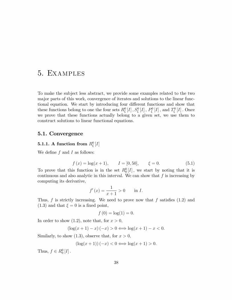
f (x) = log(x+ 1); I = [0; 50]; � = 0: (5.1)

To prove that this function is in the set R00 [I] ; we start by noting that it iscontinuous and also analytic in this interval. We can show that f is increasing bycomputing its derivative,

f 0 (x) =1

x+ 1> 0 in I:

Thus, f is strictly increasing. We need to prove now that f satis�es (1.2) and(1.3) and that � = 0 is a �xed point,

f (0) = log(1) = 0:

In order to show (1.2), note that, for x > 0;

(log(x+ 1)� x) (�x) > 0() log(x+ 1)� x < 0:Similarly, to show (1.3), observe that, for x > 0;

(log(x+ 1)) (�x) < 0() log(x+ 1) > 0:

Thus, f 2 R00 [I] :

38

x

f x

Figure 5.1: A function f 2 Rn� [I] ; as well as the boundaries y1 = x and y2 = �.

5.1.2. A function from S0� [I]

We de�ne f and I as follows:

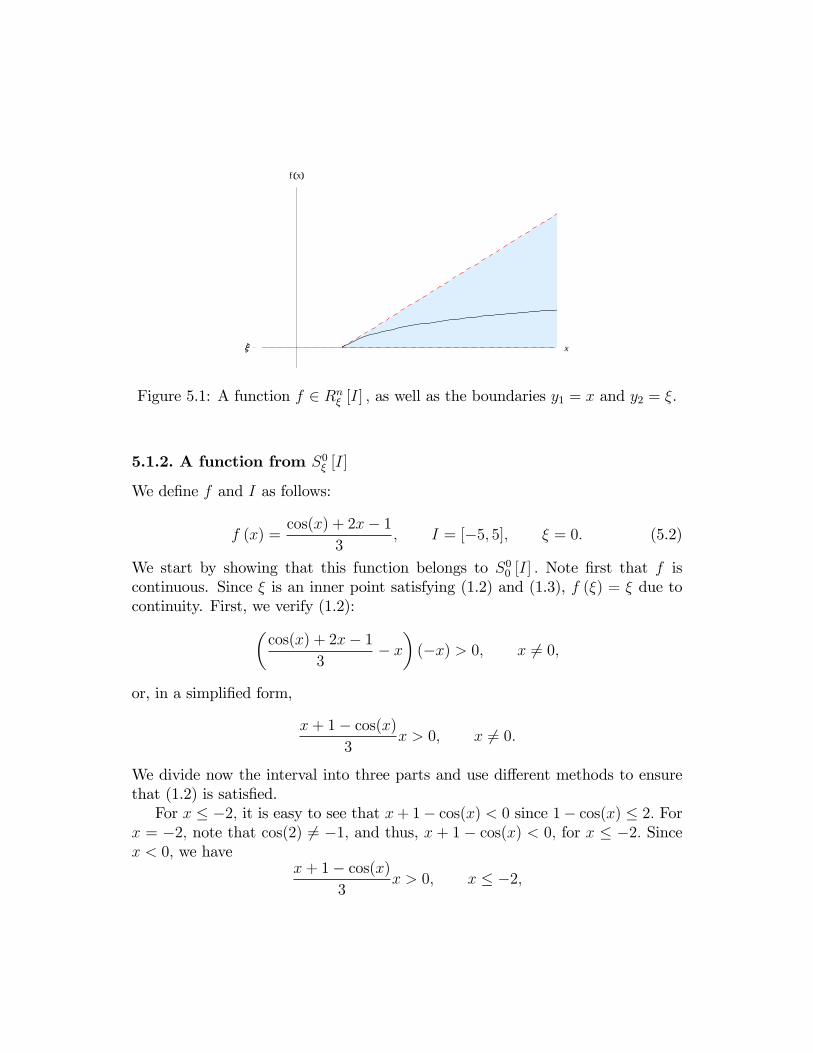
f (x) =cos(x) + 2x� 1

3; I = [�5; 5]; � = 0: (5.2)

We start by showing that this function belongs to S00 [I] : Note �rst that f iscontinuous. Since � is an inner point satisfying (1.2) and (1.3), f (�) = � due tocontinuity. First, we verify (1.2):�

cos(x) + 2x� 13

� x�(�x) > 0; x 6= 0;

or, in a simpli�ed form,

x+ 1� cos(x)3

x > 0; x 6= 0:

We divide now the interval into three parts and use di¤erent methods to ensurethat (1.2) is satis�ed.For x � �2; it is easy to see that x+ 1� cos(x) < 0 since 1� cos(x) � 2: For

x = �2; note that cos(2) 6= �1; and thus, x + 1 � cos(x) < 0; for x � �2: Sincex < 0; we have

x+ 1� cos(x)3

x > 0; x � �2;

as we wanted to prove.For �2 < x < 0; we use �rst the identity and the fact that, x 6= 0

1� cos (x) = 2�sin�x2

��2<x2

2:

Hence, get the inequality

1� cos (x) < x2

2() 1� cos (x)� x

2

2< 0:

Using this result, we have

x+ 1� cos(x)3

x >x+ 1� cos(x)

3x�

x2

2+ 1� cos(x)

3x

=x� x2

2

3x =

x2 � x3

2

3> 0; �2 < x < 0;

and we have the desired inequality.For the last case, x > 0; we note that 0 � 1� cos (x) and

x+ 1� cos(x)3

x � x+ 1� cos(x)3

x� 1� cos(x)3

x =x2

3> 0;

so (1.2) is true for all x: To check (1.3), we have to show that

cos(x) + 2x� 13

(�x) < 0; x 6= 0:

For x < 0; since 0 � cos(x)� 1; we have

cos(x) + 2x� 13

(�x) � cos(x) + 2x� 13

(�x)

� cos(x)� 13

(�x) = �2x2

3< 0:

For 0 < x < 2;

cos(x) + 2x� 13

(�x) < cos(x) + 2x� 13

(�x)

�x2

2� 1 + cos(x)

3(�x) = �

2x� x2

2

3x < 0:

For x � 2; it is easy to see that cos(x) + 2x� 1 > 0; and thus,cos(x) + 2x� 1

3(�x) < 0:

Thus, the function f satis�es (1.3) as well, hence f 2 S00 [I] :

x

f x

Figure 5.2: A function f 2 Sn� [I] ; as well as the boundaries y1 = x and y2 = �.

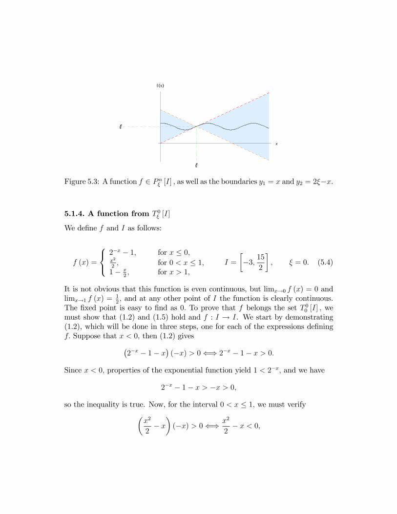
5.1.3. A function from P 0� [I]

We de�ne f and I as follows:

f (x) = sin(x); I = [�5; 5]; � = 0: (5.3)

To prove that f 2 P 00 [I] ; we need to show (1.2), (1.4) and that f : I ! I. Dueto Lemma 16, f : I ! I;. To verify (1.2), suppose that x < 0: Then,

(sin(x)� x) (�x) > 0() (sin(x)� x) > 0;

and the inequality is true for all x < 0: Suppose now that x > 0; then

(sin(x)� x) (�x) > 0() (sin(x)� x) < 0;

which is true for all x > 0: It remains to verify (1.4). Suppose �rst that x < 0; then

(sin(x) + x) (�x) < 0() (sin(x) + x) < 0;

which is true for all x < 0: Suppose now that x > 0; then

(sin(x) + x) (�x) < 0() (sin(x) + x) > 0;

and the inequality is true for all x > 0: Thus, f 2 P 00 [I] since f (x) is obviouslycontinuous.

x

f x

Figure 5.3: A function f 2 P n� [I] ; as well as the boundaries y1 = x and y2 = 2��x.

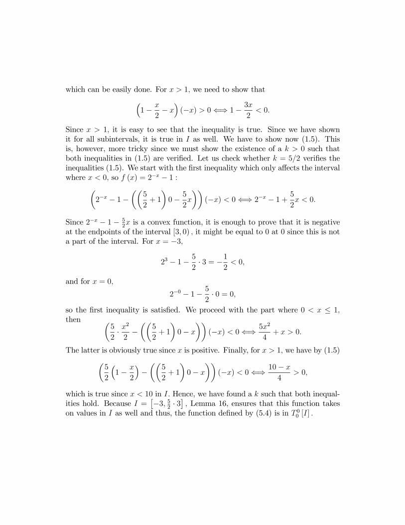
5.1.4. A function from T 0� [I]

We de�ne f and I as follows:

f (x) =

8<:2�x � 1; for x � 0;x2

2; for 0 < x � 1;

1� x2; for x > 1;

I =

��3; 15

2

�; � = 0: (5.4)

It is not obvious that this function is even continuous, but limx!0 f (x) = 0 andlimx!1 f (x) =

12; and at any other point of I the function is clearly continuous.

The �xed point is easy to �nd as 0: To prove that f belongs the set T 00 [I] ; wemust show that (1.2) and (1.5) hold and f : I ! I. We start by demonstrating(1.2), which will be done in three steps, one for each of the expressions de�ningf: Suppose that x < 0; then (1.2) gives�

2�x � 1� x�(�x) > 0() 2�x � 1� x > 0:

Since x < 0; properties of the exponential function yield 1 < 2�x; and we have

2�x � 1� x > �x > 0;

so the inequality is true. Now, for the interval 0 < x � 1; we must verify�x2

2� x�(�x) > 0() x2

2� x < 0;

which can be easily done. For x > 1; we need to show that�1� x

2� x�(�x) > 0() 1� 3x

2< 0:

Since x > 1; it is easy to see that the inequality is true. Since we have shownit for all subintervals, it is true in I as well. We have to show now (1.5). Thisis, however, more tricky since we must show the existence of a k > 0 such thatboth inequalities in (1.5) are veri�ed. Let us check whether k = 5=2 veri�es theinequalities (1.5). We start with the �rst inequality which only a¤ects the intervalwhere x < 0; so f (x) = 2�x � 1 :�

2�x � 1���

5

2+ 1

�0� 5

2x

��(�x) < 0() 2�x � 1 + 5

2x < 0:

Since 2�x � 1 � 52x is a convex function, it is enough to prove that it is negative

at the endpoints of the interval [3; 0) ; it might be equal to 0 at 0 since this is nota part of the interval. For x = �3;

23 � 1� 52� 3 = �1

2< 0;

and for x = 0;

2�0 � 1� 52� 0 = 0;

so the �rst inequality is satis�ed. We proceed with the part where 0 < x � 1;then �

5

2� x

2

2���

5

2+ 1

�0� x

��(�x) < 0() 5x2

4+ x > 0:

The latter is obviously true since x is positive. Finally, for x > 1; we have by (1.5)�5

2

�1� x

2

����

5

2+ 1

�0� x

��(�x) < 0() 10� x

4> 0;

which is true since x < 10 in I: Hence, we have found a k such that both inequal-ities hold. Because I =

��3; 5

2� 3�; Lemma 16, ensures that this function takes

on values in I as well and thus, the function de�ned by (5.4) is in T 00 [I] :

x

f x

Figure 5.4: A function f 2 T n� [I] ; as well as the boundaries y1 = x and y2 de�nedby (1.5)

5.2. Solutions to linear functional equations

We will show now some explicit solutions of linear functional equations. Since wehave de�ned in Section 5.1 four converging functions, we use them in the examples.To make it easier to follow, the examples are constructed in such a way that case(iii) is the only case that occurs, so there is always at most one solution to a givenlinear functional equation. We do this mainly for the sake of visualization. Thatis also why � = 0 in all the examples. For other values of �; one can simply movethe origin with a very simple transformation, z = x� �:

5.2.1. A function from R0� [I]

For the function (5.1), we have chosen the linear functional equation

' (log(x+ 1)) + ' (x) = sin (x) : (5.5)

We have g (x) = �1 in I and F (x) = sin (x) 2 � [I] : According to Theorem 31,equation (5.5) has a unique solution described by

' (x) = �12

F (x)

g (x)+

1Xi=1

�F (f i (x))

Gi+1 (x)+F (f i�1 (x))

Gi (x)

�!:

10 20 30 40 50x

1.5

1.0

0.5

0.5

1.0

1.5

2.0

x

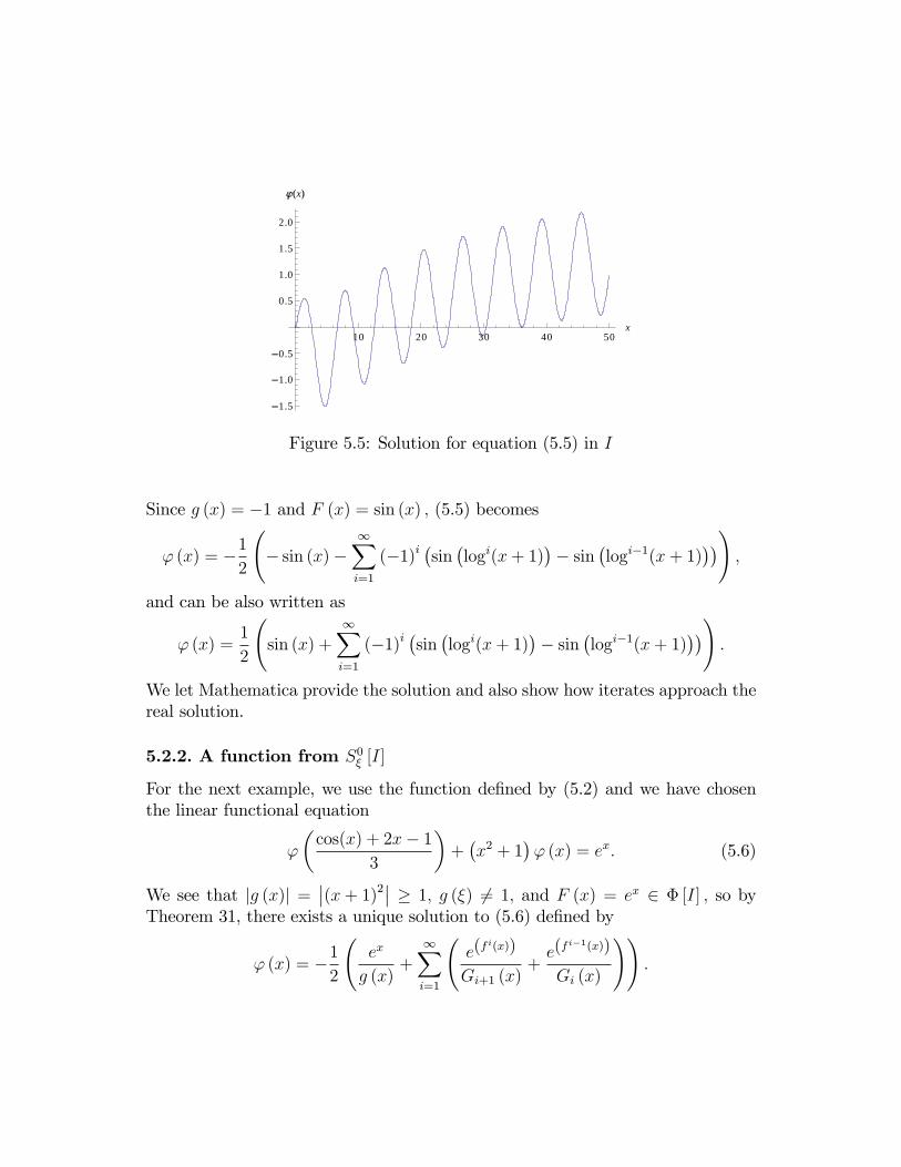
Figure 5.5: Solution for equation (5.5) in I

Since g (x) = �1 and F (x) = sin (x) ; (5.5) becomes

' (x) = �12

� sin (x)�

1Xi=1

(�1)i�sin�logi(x+ 1)

�� sin

�logi�1(x+ 1)

��!;

and can be also written as

' (x) =1

2

sin (x) +

1Xi=1

(�1)i�sin�logi(x+ 1)

�� sin

�logi�1(x+ 1)

��!:

We let Mathematica provide the solution and also show how iterates approach thereal solution.

5.2.2. A function from S0� [I]

For the next example, we use the function de�ned by (5.2) and we have chosenthe linear functional equation

'

�cos(x) + 2x� 1

3

�+�x2 + 1

�' (x) = ex: (5.6)

We see that jg (x)j =��(x+ 1)2�� � 1; g (�) 6= 1; and F (x) = ex 2 � [I] ; so by

Theorem 31, there exists a unique solution to (5.6) de�ned by

' (x) = �12

ex

g (x)+

1Xi=1

e(f

i(x))

Gi+1 (x)+e(f

i�1(x))

Gi (x)

!!:

4 2 2 4x

1

2

3

4

5

x

Figure 5.6: Solution for equation (5.6) in I

We use Mathematica to visualize the solution.

5.2.3. A function from P 0� [I]

In this case, we want to solve an equation with the function de�ned by (5.3). Wede�ne the linear functional equation as follows:

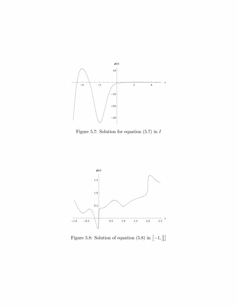
' (sin (x))� 2ex' (x) = cos (x) : (5.7)

Observe that in the case (5.7), we have g (x) = 2ex; which means that jg (�)j =2 > 1 and F (x) = cos (x) 2 � [I] ; so Theorem 31 provides the unique solution.

5.2.4. A function from T 0� [I]

The function (5.4) in T is the most complicated, but it is also continuous andde�ned in I: We use it for a linear functional equation

' (f (x)) +

e�

x2

4 (2x2 + 1)

3

!' (x) =

pjxj: (5.8)

We haveg (x) = �e�x2

4

�2x2 + 1

�;

4 2 2 4x

30

20

10

10

x

Figure 5.7: Solution for equation (5.7) in I

1.0 0.5 0.5 1.0 1.5 2.0 2.5x

0.5

1.0

1.5

x

Figure 5.8: Solution of equation (5.8) in��1; 5

2

�

In order to show that the values of g (x) for all x close to x = 0 will be less thennegative one,.we investigate the second derivative of g (x) ;

g00 (0) =�e 0

2

4 (2 � 04 + 19 � x2 + 14)4

= �72:

Since the value of the derivative is negative at 0; we have a maximum at 0 andg (0) = �1: There must therefore exist a neighborhood of 0 where g (x) � �1;so, according to Theorem 31, we have the case (iii) : Taking into account thatF 2 � [I] ; we know that there is a unique solution, and we use Mathematica togenerate the solution.

6. Conclusions

Initially, the purpose of this work was to analyze formulas describing solutions tolinear functional equations in di¤erent cases. After reading the work of Kuczma[1], I understood that the theoretical basis of the subject is much larger than I�rst presumed. Furthermore, a good starting point for the project was to de�nefunctions that converge to a �xed point. Therefore, this paper is divided into twomajor parts, the �rst, where the purpose is to expand the sets with the convergenceproperty, and the second, where the work of Kuczma [1] is partly adjusted to beused with these new sets. Since the theory of functional equations is not discussedin mathematical courses at a bachelor level, I had no notable understanding forthe subject before this work. However, much of the theory in [1] is presented ina way that a student with some experience in analysis, di¤erential equations andset theory is able to comprehend. Personally, I believe that I have got a muchwider perspective not only on the subject of functional equations, but also ona more general mathematical �eld of analysis, especially on the ways of solvingmathematical problems with a non-direct approach through the development ofthe corresponding theory around the subject.Despite being largely based on Marek Kuczma�s book [1], this work provides

also examples and historical facts related to functional equations along with thematerial related to iterative solutions from the book by Small [2] and websites[3]. A very important source of information is the book [2]. It provided an ideaon how to transform some general functional equations to linear, as well as aformula to work with exponents. As a �nal statement, I can say that even thoughapplications of functional equations is another interesting part of the subject, ithas not been presented here due to a mostly theoretical standpoint of this report.

49

Bibliography

[1] Marek Kuczma, Functional Equations in a Single Variable, Polish Scienti�cPublishers, Warszawa, 1968

[2] Christopher G. Small, Functional Equations and How to Solve Them, Springer,New York, 2007

[3] http://eqworld.ipmnet.ru/en/solutions/fe/fe1208.pdf

[4] http://en.wikipedia.org/wiki/Gr%C3%A9goire_de_Saint-Vincent

[5] http://commons.wikimedia.org/wiki/File:CharlesBabbage.jpg

[6] http://ste�zu.wordpress.com/augustin-louis-cauchy-3

50

7. Appendix

See separate document: Appendix

51

Exit@D

R

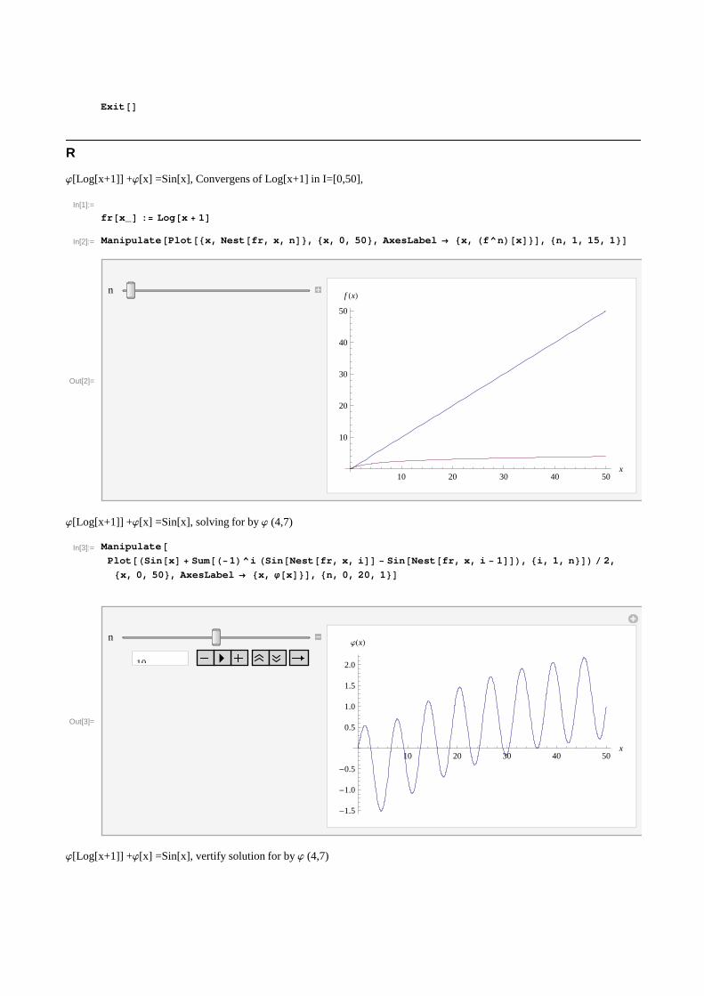
j[Log[x+1]] +j[x] =Sin[x], Convergens of Log[x+1] in I=[0,50],

In[1]:=

fr@x_D := Log@x + 1D

In[2]:= Manipulate@Plot@8x, Nest@fr, x, nD<, 8x, 0, 50<, AxesLabel ® 8x, Hf^nL@xD<D, 8n, 1, 15, 1<D

Out[2]=

n

10 20 30 40 50x

10

20

30

40

50

f HxL

j[Log[x+1]] +j[x] =Sin[x], solving for by j (4,7)

In[3]:= Manipulate@Plot@HSin@xD + Sum@H-1L^i HSin@Nest@fr, x, iDD - Sin@Nest@fr, x, i - 1DDL, 8i, 1, n<DL � 2,

8x, 0, 50<, AxesLabel ® 8x, j@xD<D, 8n, 0, 20, 1<D

Out[3]=

n

10

10 20 30 40 50x

-1.5

-1.0

-0.5

0.5

1.0

1.5

2.0

jHxL

j[Log[x+1]] +j[x] =Sin[x], vertify solution for by j (4,7)

In[4]:=

Manipulate@Plot@8Sin@xD, HSin@fr@xDD +

Sum@H-1L^i HSin@Nest@fr, fr@xD, iDD - Sin@Nest@fr, fr@xD, i - 1DDL, 8i, 1, n<DL � 2 +

HSin@xD + Sum@H-1L^i HSin@Nest@fr, x, iDD - Sin@Nest@fr, x, i - 1DDL, 8i, 1, n<DL � 2<,8x, 0, 50<, AxesLabel ® 8x, F@xD<D, 8n, 0, 20, 1<D

Out[4]=

n

10 20 30 40 50x

-1.0

-0.5

0.5

1.0

FHxL

¢ | £

2 Examples.nb

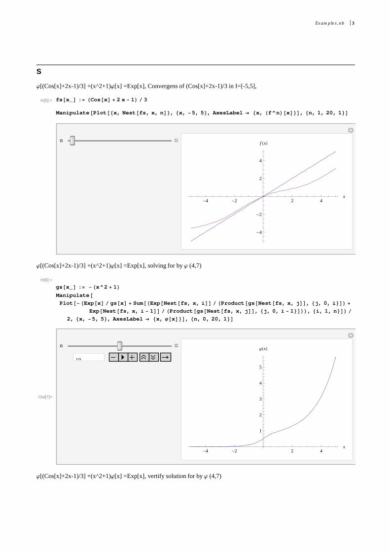
S

j[(Cos[x]+2x-1)/3] +(x^2+1)j[x] =Exp[x], Convergens of (Cos[x]+2x-1)/3 in I=[-5,5],

In[5]:= fs@x_D := HCos@xD + 2 x - 1L � 3

Manipulate@Plot@8x, Nest@fs, x, nD<, 8x, -5, 5<, AxesLabel ® 8x, Hf^nL@xD<D, 8n, 1, 20, 1<D

n

-4 -2 2 4x

-4

-2

2

4

f HxL

j[(Cos[x]+2x-1)/3] +(x^2+1)j[x] =Exp[x], solving for by j (4,7)

In[6]:=

gs@x_D := -Hx^2 + 1LManipulate@Plot@-HExp@xD � gs@xD + Sum@HExp@Nest@fs, x, iDD � HProduct@gs@Nest@fs, x, jDD, 8j, 0, i<DL +

Exp@Nest@fs, x, i - 1DD � HProduct@gs@Nest@fs, x, jDD, 8j, 0, i - 1<DLL, 8i, 1, n<DL �2, 8x, -5, 5<, AxesLabel ® 8x, j@xD<D, 8n, 0, 20, 1<D

Out[7]=

n

10

-4 -2 2 4x

1

2

3

4

5

jHxL

j[(Cos[x]+2x-1)/3] +(x^2+1)j[x] =Exp[x], vertify solution for by j (4,7)

Examples.nb 3

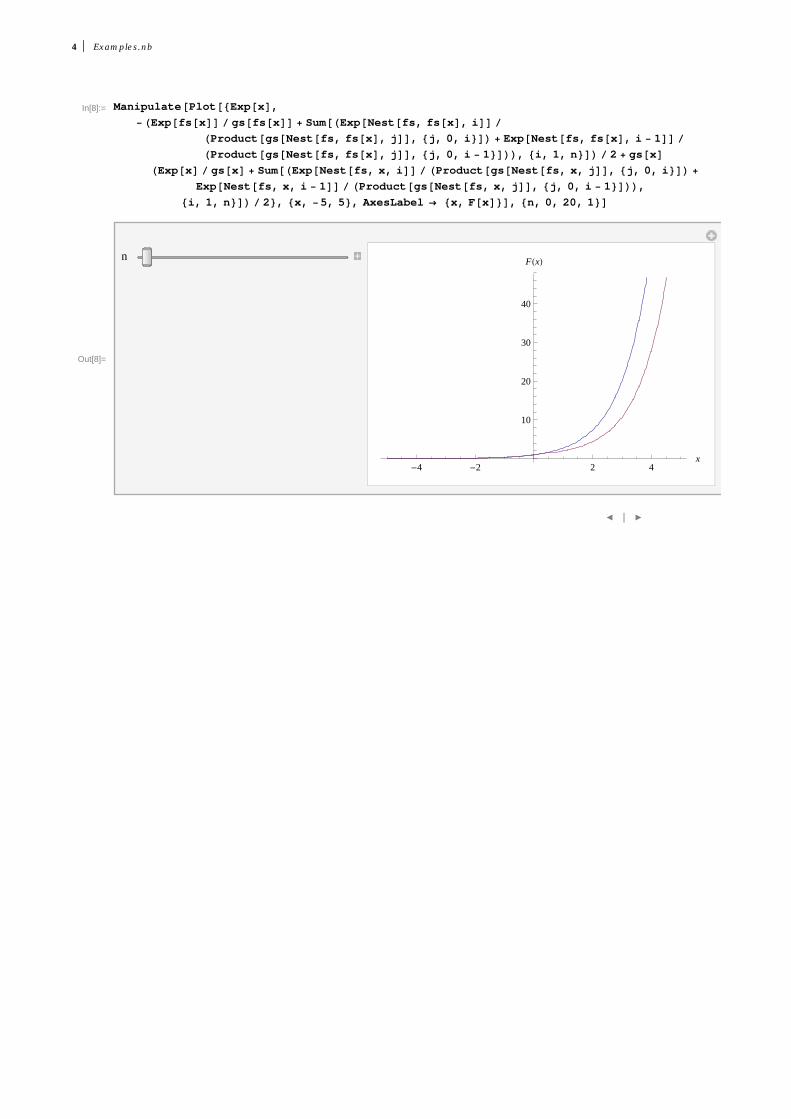
In[8]:= Manipulate@Plot@8Exp@xD,-HExp@fs@xDD � gs@fs@xDD + Sum@HExp@Nest@fs, fs@xD, iDD �

HProduct@gs@Nest@fs, fs@xD, jDD, 8j, 0, i<DL + Exp@Nest@fs, fs@xD, i - 1DD �HProduct@gs@Nest@fs, fs@xD, jDD, 8j, 0, i - 1<DLL, 8i, 1, n<DL � 2 + gs@xD

HExp@xD � gs@xD + Sum@HExp@Nest@fs, x, iDD � HProduct@gs@Nest@fs, x, jDD, 8j, 0, i<DL +

Exp@Nest@fs, x, i - 1DD � HProduct@gs@Nest@fs, x, jDD, 8j, 0, i - 1<DLL,8i, 1, n<DL � 2<, 8x, -5, 5<, AxesLabel ® 8x, F@xD<D, 8n, 0, 20, 1<D

Out[8]=

n

-4 -2 2 4x

10

20

30

40

FHxL

¢ | £

4 Examples.nb

P

j[Sin[x]] -2Exp[x]j[x] =Cos[x], Convergens of Sin[x] in I=[-5,5],

In[9]:= fp@x_D := Sin@xDManipulate@Plot@8x, -x, Nest@fp, x, nD<, 8x, -5, 5<, AxesLabel ® 8x, Hf^nL@xD<D, 8n, 1, 20, 1<D

Out[10]=

n

-4 -2 2 4x

-4

-2

2

4

f HxL

j[Sin[x]] -2Exp[x]j[x] =Cos[x], solving for by j (4,7)

In[11]:= gp@x_D := 2 Exp@xDManipulate@Plot@-HCos@xD � gp@xD + Sum@HCos@Nest@fp, x, iDD � HProduct@gp@Nest@fp, x, jDD, 8j, 0, i<DL +

Cos@Nest@fp, x, i - 1DD � HProduct@gp@Nest@fp, x, jDD, 8j, 0, i - 1<DLL, 8i, 1, n<DL �2, 8x, -5, 5<, AxesLabel ® 8x, j@xD<D, 8n, 0, 20, 1<D

Out[12]=

n

10

-4 -2 2 4x

-30

-20

-10

10

jHxL

j[Sin[x]] -2Exp[x]j[x] =Cos[x], vertify solution for by j (4,7)

Examples.nb 5

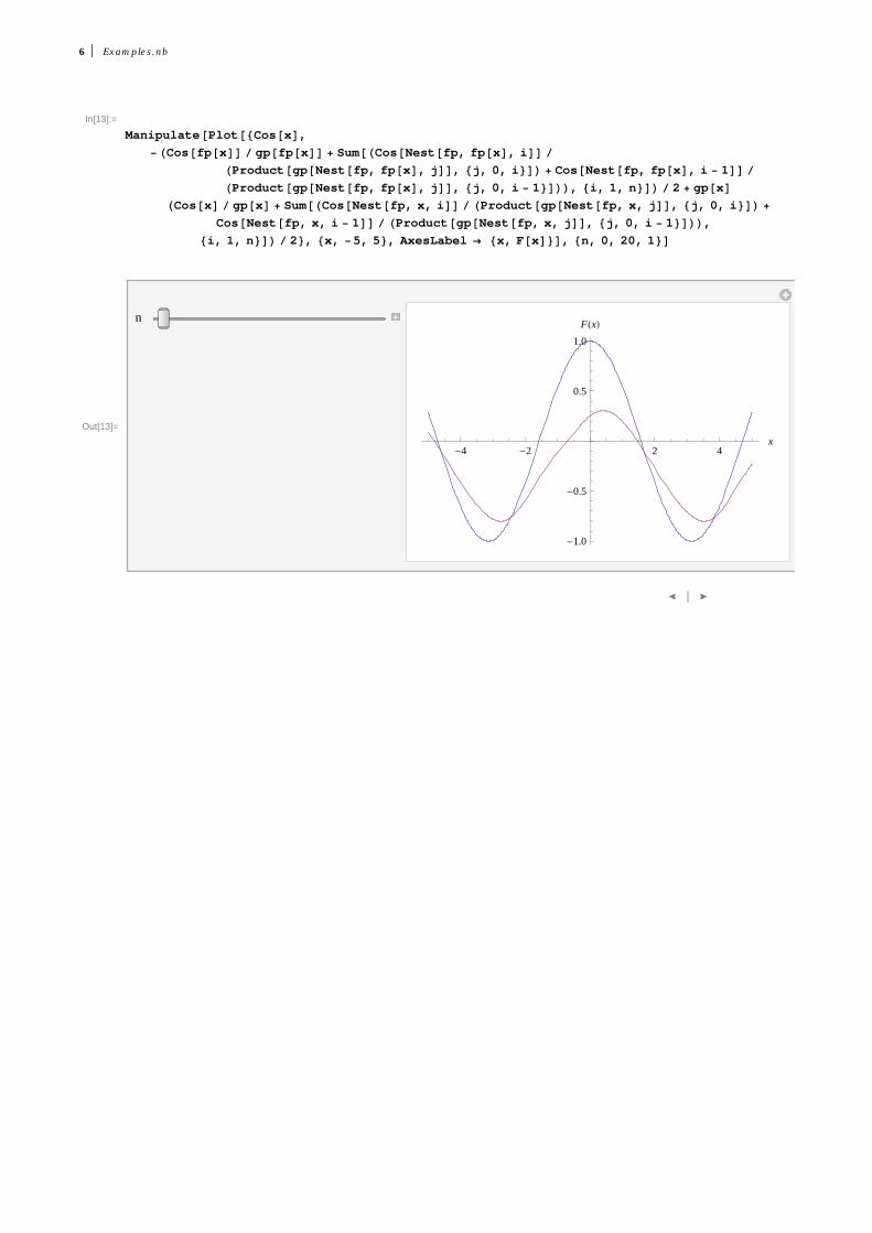
In[13]:=

Manipulate@Plot@8Cos@xD,-HCos@fp@xDD � gp@fp@xDD + Sum@HCos@Nest@fp, fp@xD, iDD �

HProduct@gp@Nest@fp, fp@xD, jDD, 8j, 0, i<DL + Cos@Nest@fp, fp@xD, i - 1DD �HProduct@gp@Nest@fp, fp@xD, jDD, 8j, 0, i - 1<DLL, 8i, 1, n<DL � 2 + gp@xD

HCos@xD � gp@xD + Sum@HCos@Nest@fp, x, iDD � HProduct@gp@Nest@fp, x, jDD, 8j, 0, i<DL +

Cos@Nest@fp, x, i - 1DD � HProduct@gp@Nest@fp, x, jDD, 8j, 0, i - 1<DLL,8i, 1, n<DL � 2<, 8x, -5, 5<, AxesLabel ® 8x, F@xD<D, 8n, 0, 20, 1<D

Out[13]=

n

-4 -2 2 4x

-1.0

-0.5

0.5

1.0

FHxL

¢ | £

6 Examples.nb

T

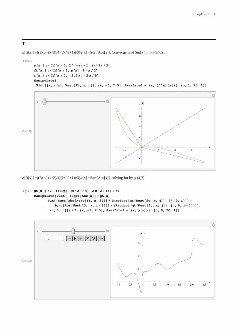
j[ft[x]] +((Exp[-(x^2)/4](2x^2+1))/3)j[x] =Sqrt[Abs[x]], Convergens of Sin[x] in I=[-3,7.5],

In[14]:=

p@x_D := If@x < 0, 2^H-xL - 1, Hx^2L � 2Dft@x_D := If@x < 1, p@xD, 1 - x � 2Dr@x_D := If@x < 0, -2.5 x, -2 x � 5DManipulate@Plot@8x, r@xD, Nest@ft, x, nD<, 8x, -3, 7.5<, AxesLabel ® 8x, Hf^nL@xD<D, 8n, 1, 20, 1<D

Out[17]=

n

-2 2 4 6x

-2

2

4

6

f HxL

j[ft[x]] +((Exp[-(x^2)/4](2x^2+1))/3)j[x] =Sqrt[Abs[x]], solving for by j (4,7)

In[18]:= gt@x_D := -HHExp@-Hx^2L � 4D H2 x^2 + 1LL � 3LManipulate@Plot@-HSqrt@Abs@xDD � gt@xD +

Sum@HSqrt@Abs@Nest@ft, x, iDDD � HProduct@gt@Nest@ft, x, jDD, 8j, 0, i<DL +

Sqrt@Abs@Nest@ft, x, i - 1DDD � HProduct@gt@Nest@ft, x, jDD, 8j, 0, i - 1<DLL,8i, 1, n<DL � 2, 8x, -1, 2.5<, AxesLabel ® 8x, j@xD<D, 8n, 0, 20, 1<D

Out[19]=

n

10

-1.0 -0.5 0.5 1.0 1.5 2.0 2.5x

0.5

1.0

1.5

jHxL

Examples.nb 7

10

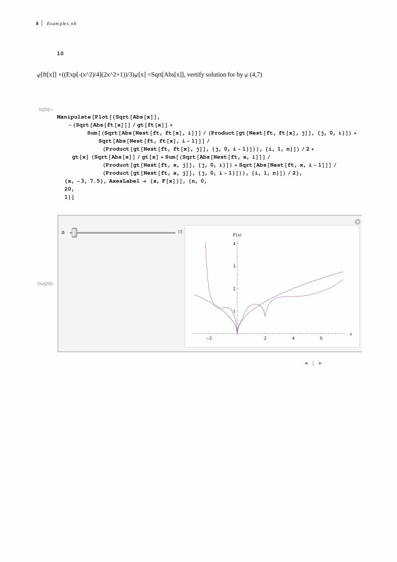
j[ft[x]] +((Exp[-(x^2)/4](2x^2+1))/3)j[x] =Sqrt[Abs[x]], vertify solution for by j (4,7)

In[20]:=

Manipulate@Plot@8Sqrt@Abs@xDD,-HSqrt@Abs@ft@xDDD � gt@ft@xDD +

Sum@HSqrt@Abs@Nest@ft, ft@xD, iDDD � HProduct@gt@Nest@ft, ft@xD, jDD, 8j, 0, i<DL +

Sqrt@Abs@Nest@ft, ft@xD, i - 1DDD �HProduct@gt@Nest@ft, ft@xD, jDD, 8j, 0, i - 1<DLL, 8i, 1, n<DL � 2 +

gt@xD HSqrt@Abs@xDD � gt@xD + Sum@HSqrt@Abs@Nest@ft, x, iDDD �HProduct@gt@Nest@ft, x, jDD, 8j, 0, i<DL + Sqrt@Abs@Nest@ft, x, i - 1DDD �HProduct@gt@Nest@ft, x, jDD, 8j, 0, i - 1<DLL, 8i, 1, n<DL � 2<,

8x, -3, 7.5<, AxesLabel ® 8x, F@xD<D, 8n, 0,

20,

1<D

Out[20]=

n

-2 2 4 6x

1

2

3

4

FHxL

¢ | £

8 Examples.nb