Embed Size (px)
Citation preview
LINEAR AND NONLINEAR FLEXURAL STIFFNESS MODELS
FOR CONCRETE WALLS IN HIGH-RISE BUILDINGS
by
AhmedM. M. Ibrahim
B.Sc, Cairo University, Cairo, 1990
M.A.Sc , Concordia University, Montreal, 1995
A THESIS SUBMITTED IN PARTIAL FULFILMENT OF
THE REQUIREMENTS FOR THE DEGREE OF
Doctor of Philosophy
in
The Faculty of Graduate Studies
Department of Civil Engineering
We accept this thesis as conforming to the required standard
THE UNIVERSITY OF BRITISH COLUMBIA
October 2000
© Ahmed Ibrahim, 2000
In presenting this thesis in partial fulfilment of the requirements for an advanced
degree at the University of British Columbia, I agree that the Library shall- make it
freely available for reference and study. I further agree that permission for extensive
copying of this thesis for scholarly purposes may be granted by the head of my
department or by his or her representatives. It is understood that copying or
publication of this thesis for financial gain shall not be allowed without my written
permission.
Department of f l\i>L c v y ^ ' i v u ^
The University of British Columbia Vancouver, Canada
DE-6 (2/88)

r
ABSTRACT In the seismic design of high-rise wall buildings, the fundamental period of the building and the
building drift are usually determined using linear elastic dynamic analysis. To carry out this
analysis, designers need to assume a linear flexural stiffness of the wall sections that account for
cracking. The commentary to the 1994 Canadian concrete code (CPCA 1995) suggests a stiffness
value of 70% of the gross moment of inertia (Ig) of the wall section. The commentary to the
1995 New Zealand Standard (NZS 3101 1995) suggests much lower stiffness values. A wall
subjected to axial compression of 10% of fj Ag is suggested to have half what is recommended
in the CPCA Handbook (i.e. 0.35 Ig). The NEHRP Guidelines for the Seismic Rehabilitation of
Buildings (FEMA 273) suggests stiffness values of 0.8 Ig and 0.5 Ig for uncracked and cracked
concrete walls, respectively. While it is not clear which of the recommended stiffness values
should be used, it is certainly clear that the choice of stiffness value will have a significant
influence on the predicted period and drift of the building.
The actual influence of cracking on the flexural stiffness of a concrete wall subjected to seismic
loading is nonlinear. Nonlinear static analysis is increasingly used to capture this influence
provided that an appropriate nonlinear model is used for the material.
In this thesis, a simple nonlinear flexural (bending moment-curvature) model for concrete walls
in high-rise buildings is proposed. To validate the model, a 40 ft high slender concrete wall was
constructed and tested under simulated earthquake loading. Results from the test were compared
with the proposed model and showed good agreement. Based on the proposed piece-wise linear
model, a general method to determine the linear "effective" flexural stiffness of concrete walls
was developed. Results from the general method for the effective flexural stiffness showed that
the large variation in effective stiffness that is recommended by various design guidelines does
actually exist for different wall configurations under certain conditions. The general method
presented in this thesis gives the appropriate stiffness for a particular wall considering all
important parameters that influence the stiffness. A study was conducted to examine the
influence of a variety of parameters on the stiffness of concrete walls and a set of simplified
expressions are proposed for the effective flexural stiffness of concrete walls.
(ii)

The piece-wise flexural model is implemented into a nonlinear static (pushover) analysis
computer program to demonstrate the use of the model in predicting the nonlinear static response
of concrete walls. Two example applications are presented, including the analysis of a 450 ft
high coupled wall structure currently being constructed. The results from the analysis showed the
importance of accurately modeling the nonlinear flexural stiffness of concrete walls.
(iii)
Table of Contents
ABSTRACT ii
TABLE OF CONTENTS zv
LIST OF TABLES vii
LIST OF FIGURES viii
ACKNOWLEDGEMENTS xii
DEDICATION xiii
1 INTRODUCTION
1.1 Concrete Structural Walls 1
1.2 Seismic Analysis of Buildings 2
1.3 Objectives of Thesis 5
1.4 Organization of Thesis 6
2 NONLINEAR FLEXURAL STIFFNESS MODEL FOR CONCRETE WALLS
2.1 Introduction 7
2.2 Typical Bending Moment-Curvature Relationship of a Wall Section 8
2.3 Tensile Stresses of Cracked Concrete 10
2.4 Bending Moment-Curvature Response Under Monotonic Loading 15
2.5 Bending Moment-Curvature Response Under Cyclic Loading 18
2.6 Trilinear Bending Moment-Curvature Relationship for Concrete Walls... 19
2.6.1 Slope of the Linear Elastic Response, EJg 19
2.6.2 Slope of the Second Linear Segment, EJcr 22
2.6.3 Flexural Capacity, M„ 24
2.6.4 Linear Bending Moment, Mi 24
2.7 Concluding Remarks 32
3 EXPERIMENTAL STUDY OF A LARGE-SCALE SLENDER WALL
3.1 General 35
3.2 Description of Test Specimen 35
(iv)
3.3 Test Set-up 40
3.4 Instrumentation 40
3.5 Test Procedure 43
3.6 Corrections to Measured Results 46
3.7 Summary of Test Observations 49
3.8 Discussion of Test Results 49
3.9 Comparison with the Trilinear Bending Moment-Curvature Model 54
3.10 Concluding Remarks 55
4 EFFECTIVE FLEXURAL STIFFNESS OF CONCRETE WALLS
4.1 Introduction 59
4.2 Prediction of the Load-Displacement Relationship 61
4.3 Characteristics of the Load-Displacement Relationship 63
4.4 Determination of Effective Flexural Stiffness of Concrete Walls 66
4.5 Trend of Stiffness Variation 73
4.5.1 Axial Compression Acting on the Wall 73
4.5.2 Geometry of the Wall Section 74
4.5.3 Amount and Distribution of the Vertical Reinforcement 77
4.5.4 Concrete Compressive Strength 78
4.5.5 Yield Strength of the Vertical Reinforcement 83
4.6 Recommendations for Effective Flexural Stiffness of Concrete Walls 86
4.6.1.1 General Methodfor Determining Effective Flexural Stiffness 86
4.6.2 Simplified Method for Determining the Effective Flexural
Stiffness 87
4.7 Comparison of Predicted Stiffness with Slender Wall Test Results 96
4.8 Concluding Remarks 97
5 NONLINEAR STATIC ANALYSIS OF CONCRETE WALLS
5.1 Introduction 101
5.2 Overview of the Pushover Analysis Procedure 102
5.3 Implementation of Trilinear Bending Moment-Curvature Model in
Pushover Analysis 104
(v)

5.3.1 Material Modeling 104
5.3.2 Determination of Effective Member Stiffness 106
5.3.3 Solution of the Nonlinear Equations 106
5.3.4 Plastic Hinge Formation 108
5.4 Example Applications of the Pushover Analysis 110
5.4.1 Wall Test Example 110
5.4.2 Coupled Wall Example 115
6 CONCLUSIONS AND RECOMMENDATIONS
6.1 Summary and Conclusions 123
6.2 Recommendations for Further Work 126
REFERENCES 128
APPENDIX A Plane Sections Analysis Procedure 131
APPENDIX B Bending Moment-Curvature Relationship Considering Residual
Strains due to Cyclic Loading 134
APPENDIX C Determination of Cracked Section Moment of Inertia, ICT, for a
General Flanged Wall Section 136
APPENDIX D Determination of Linear Bending Moment, Mi 139
APPENDIX E Additional Analyses to Justify Proposed Simplified Method 141
APPENDIX F Computational Procedure for Determining Effective Member
Stiffness 148
APPENDIX G Program Wall-Tools 152
(vi)

LIST OF TABLES
Table Page
4.1 Values of the exponent a and b for Equation [4.2] 70
(vii)

LIST OF FIGURES
Figure Page
1.1 Comparison of different recommendations for the effective flexural stiffness of concrete walls 4
2.1 Bending moment - curvature relationships for reinforced concrete members: (a) some simple piece-wise linear models compared to the actual nonlinear curve, (b) bilinear model suggested by Priestley and Kowalsky 1998 9
2.2 Typical bending moment - curvature relationship for a wall section in a high-rise building 11
2.3 Bending moment - curvature relationships for: (a) a typical rectangular wall in a high-rise building, (b) a typical bridge pier 12
2.4 Tension stiffening effect of a cracked reinforced concrete wall element 14 2.5 Response of concrete in tension (experimental results from Fronteddu,
1993): (a) monotonic loading (predicted and observed), (b) cyclic loading, (c) proposed model for cyclic loading 16
2.6 Bending moment-curvature relationships for typical concrete walls subjected to monotonic loading: (a) influence of axial load, (b) influence of reinforcement amount 17
2.7 Predicted influence of cyclic loading on: (a) bending moment - curvature relationship of a typical concrete wall, (b) the tension stress-strain relationship for the most highly strained concrete in the wall 20
2.8 Upper-bound and lower-bound trilinear approximations to the bending moment - curvature relationship for a typical concrete wall subjected to cyclic loading 21
2.9 Cracked section moment of inertia, Icr, for: (a) rectangular wall sections, and (b) flanged wall sections 23
2.10 Procedure to determine the flexural capacity, M„, of a typical wall section.... 25 2.11 Linear approximations to the axial load - bending moment interaction
diagrams for the upper-bound and lower-bound Mi values 28 2.12 Various concrete wall shapes considered in the determination of a simple
expression for Mi 30 2.13 Determination of the slope, a, of the linear expression for Mi 31 2.14 Determination of the intercept, /?, of the linear expression for Mi 31 2.15 Comparison of Mi determined using the simple expression (Eq. [2.7]) with
the value determined using the more rigorous method 33 2.16 Comparison of the actual nonlinear bending moment - curvature
relationships with the proposed trilinear model for typical wall sections 34
3.1 Prototype wall specimen considered for testing under cyclic loading (3.28 ft = 1 m) •. 36
3.2 Cross sectional dimensions and reinforcement details of the 40' wall test specimen 36
3.3 Large-scale slender wall test undertaken to validate the proposed trilinear model 38
3.4 Schematic of the slender wall test set-up (from Bryson 2000) 39
(viii)

3.5 Teflon sliding bearings supporting the slender wall specimen tested in a horizontal position 41
3.6 Instrumentation used to measure the response of the slender wall specimen (from Bryson 2000) 42
3.7 Measuring concrete strains at various locations along the wall height: (a) metal targets epoxyed to concrete, (b) digital caliper device 44
3.8 Sequence of imposed reverse cyclic lateral displacement at the tip of the wall 45
3.9 Measured lateral load-displacement response of the slender wall specimen... 47 3.10 (a) Correction to measured displacement due to observed rotation of the
base block during testing, (b) Correction to measured force due to Teflon sliding bearings 48
3.11 Corrected load-displacement response of the slender wall test 50 3.12 Upper-bound and lower-bound load-displacement response of the wall
specimen under cyclic loading 52 3.13 Measured bending moment-rotation response of the wall specimen taken at
the peak lateral displacement 53 3.14 Measured curvature distribution along the wall height during the different
lateral displacement cycles. 56 3.15 Trend of the measured bending moment-curvature relationship taken at
various locations along the wall height during the different lateral displacement cycles 57
3.16 Comparison of the measured and predicted bending moment-curvature relationships 58
4.1 Typical lengthening of the fundamental period of a concrete wall due to the reduction in stiffness resulting from cracking during earthquake motion 60
4.2 Procedure used to predict the load-displacement relationship: (a) assumed load distribution, (b) corresponding bending moment distribution, (c) assumed axial compression, (d) linear moment capacity, (e) resulting curvature distribution, (f) trilinear bending moment-curvature models, (g) complete load-displacement curve 62
4.3 Load-displacement characteristics for typical wall sections 65 4.4 Independent bilinear idealization of the load-displacement relationship 67 4.5 Determination of the effective flexural stiffness, Ie, for concrete walls 69 4.6 Comparison of the predicted effective flexural stiffness with the value
estimated using Eq. [4.2] 71 4.7 Comparison of the effective flexural stiffness determined using different
methods to obtain the equivalent bilinear elastic stiffness 72 4.8 Variation of the effective flexural stiffness with the magnitude of axial
compression 75 4.9 Variation of the effective flexural stiffness for different wall shapes 76 4.10 Variation of the effective flexural stiffness with different amounts of vertical
reinforcement in a rectangular wall 79 4.11 Load-displacement characteristics of a rectangular wall with different
amounts of vertical reinforcement 80 4.12 Variation of the effective flexural stiffness for flanged walls with different
amounts of vertical reinforcement 81
(ix)
4.13 Variation of the effective flexural stiffness with different distributions of the vertical reinforcement in the boundary zone of the cross section 82
4.14 Variation of the effective flexural stiffness with varying concrete compressive strength 84
4.15 Variation of the effective flexural stiffness with varying yield strength of the vertical reinforcement 85
4.16 Design chart for the determination of the effective flexural stiffness, Ie, for concrete walls using the general method 88
4.17 Comparison of the suggested simplified expressions for determining the effective flexural stiffness with a variety of results for rectangular walls 90
4.18 Comparison of the suggested simplified expressions for determining the effective flexural stiffness with a variety of results for flanged walls 91
4.19 Comparison of the suggested simplified expressions for determining the effective flexural stiffness with a variety of "T" shaped walls (flange in tension) 92
4.20 Comparison of the suggested simplified expressions for determining the effective flexural stiffness with a variety of "T" shaped walls (flange in compression) 93
4.21 Comparison of the suggested simplified expressions for determining the effective flexural stiffness with a variety of "C" shaped walls (flange in tension) 94
4.22 Comparison of the suggested simplified expressions for determining the effective flexural stiffness with a variety of "C" shaped walls (flange in compression) 95
4.23 Comparison of the experimentally measured load-displacement relationship with the one predicted using linear elastic stiffness as proposed by the general method 98
4.24 Comparison of the experimentally measured load-displacement relationship with the one predicted using the linear elastic stiffness suggested in the CPCA Handbook (1995) 99
4.25 Comparison of the experimentally measured load-displacement relationship with the one predicted using the linear elastic stiffness suggested by the commentary to NZS 3101 (1995) 100
5.1 (a) Family of idealized bending moment-curvature relationships, (b) interaction diagrams input to nonlinear pushover program 105
5.2 Application of trilinear bending moment-curvature model in nonlinear static analysis: (a) bending moment distribution in a wall element, (b) trilinear bending moment-curvature model, (c) curvature distribution in a wall element 107
5.3 Successive approximation method for a single variable 109 5.4 Trilinear bending moment-curvature relationship used for the analysis of the
slender wall specimen 112 5.5 Comparison of predicted and observed upper-bound response of the slender
wall specimen 113 5.6 Comparison of predicted and observed lower-bound response of the slender
wall specimen 114 5.7 (a) Isometric view of the core wall example, (b) cross section dimensions
(3.28ft = lm) 117
(x)
5.8 (a) Two-dimensional plane frame model subjected to first mode loading, (b) coupling beam shear capacity and demand 118
5.9 Interaction diagrams for the four core walls and used for input to the pushover analysis 119
5.10 Sequence of yielding of the different members in the two-dimensional frame model 121
5.11 Predicted nonlinear static response of 450 ft high coupled walls 122
(xi)

ACKNOWLEDGMENTS
The author is indebted to Dr. Perry Adebar for his supervision, guidance, encouragement and
constructive criticism throughout all stages of the research program. His willingness to help in
every possible way is greatly appreciated.
Thanks are due to Mr. M. Bryson for his part in the experimental investigation carried out in this
thesis.
Thanks are also due to the technical staff at the Structures Laboratory of The University of
British Columbia.
Financial assistance provided by "BC GREAT Scholarship" in collaboration with Mr. Jim
Mutrie, principal of Jones, Kwong, Kishi, and Dr. Ron DeVall, principal of Read, Jones,
Christofferesen Ltd., is greatly appreciated.
(xii)

To
Mokhtar, Fayza, Rania,
Omar and Salma
(xiii)

Chapter 1
Introduction
1.1 Concrete Structural Walls
Reinforced concrete structural walls, or shear walls, are the most commonly used system to resist
lateral motions due to earthquakes in high-rise buildings on the west coast of Canada. Concrete
walls have also been gaining in popularity in other parts of North America, particularly after
steel moment resisting frames were found to have suffered serious weld failures during the 1994
Northridge Earthquake.
Meigs et al. (1993) surveyed numerous structural engineering consultants in the United States
and Canada and cited the preference of structural wall systems when designing for earthquake
resistance due to the "excellent performance in past earthquakes, ability to minimize lateral drift,
and simplicity of design". Observations of buildings during earthquakes showed the superior
performance of those with walls as the primary lateral load resisting system compared to those
with other types of systems, particularly with regard to damage control, overall safety and
integrity of the structure (Fintel 1991, Wallace and Moehle 1992, Saatcioglu and Bruneau,
1993).
In recent years, seismic design methodologies have put greater attention on limiting the
maximum drift experienced by a structure during earthquake motions. Also, it is essential to
protect the non-seismic structural systems, i.e. other structural components in the building that
resist gravity forces, and the nonstructural elements such as windows, pipes, etc. Structural walls
possess very large in-plane stiffness and provide excellent drift control. From the point of view
of economy and drift control, structural walls may become imperative for tall buildings (Paulay
and Priestley 1992).
Concrete walls are sometimes categorized into two different types: isolated cantilever walls and
coupled walls. As the name suggests, isolated cantilever walls are relatively independent of
other walls as the concrete slabs that connect the walls together are not capable of transmitting
1
2
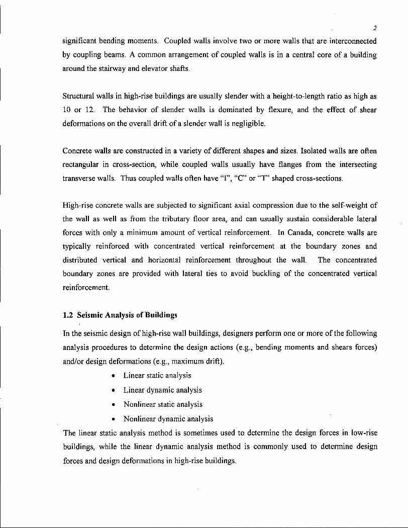
significant bending moments. Coupled walls involve two or more walls that are interconnected
by coupling beams. A common arrangement of coupled walls is in a central core of a building
around the stairway and elevator shafts.
Structural walls in high-rise buildings are usually slender with a height-to-length ratio as high as
10 or 12. The behavior of slender walls is dominated by flexure, and the effect of shear
deformations on the overall drift of a slender wall is negligible.
Concrete walls are constructed in a variety of different shapes and sizes. Isolated walls are often
rectangular in cross-section, while coupled walls usually have flanges from the intersecting
transverse walls. Thus coupled walls often have "I", "C" or "T" shaped cross-sections.
High-rise concrete walls are subjected to significant axial compression due to the self-weight of
the wall as well as from the tributary floor area, and can usually sustain considerable lateral
forces with only a minimum amount of vertical reinforcement. In Canada, concrete walls are
typically reinforced with concentrated vertical reinforcement at the boundary zones and
distributed vertical and horizontal reinforcement throughout the wall. The concentrated
boundary zones are provided with lateral ties to avoid buckling of the concentrated vertical
reinforcement.
1.2 Seismic Analysis of Buildings
In the seismic design of high-rise wall buildings, designers perform one or more of the following
analysis procedures to determine the design actions (e.g., bending moments and shears forces)
and/or design deformations (e.g., maximum drift).
• Linear static analysis
• Linear dynamic analysis
• Nonlinear static analysis
• Nonlinear dynamic analysis
The linear static analysis method is sometimes used to determine the design forces in low-rise
buildings, while the linear dynamic analysis method is commonly used to determine design
forces and design deformations in high-rise buildings.

3
To perform a linear dynamic analysis, designers need to assume an effective flexural stiffness of
the concrete wall elements. The flexural stiffness of an uncracked wall is equal to EcIg where Ec
is the modulus of elasticity of concrete, and Ig is the moment of inertia of the gross (uncracked)
concrete section. Once concrete cracks, the flexural stiffness reduces depending on the extent of
cracking and the amount of vertical reinforcement. An average (effective) stiffness Ec Ie less
than the uncracked stiffness is normally used in linear dynamic analysis to account for the effects
of cracking.
The commentary to the 1994 Canadian concrete code (CPCA, 1995) suggests using an effective
moment of inertia Ie equal to 70% of the gross moment of inertia Ig of the wall section. The
commentary to the 1995 New Zealand concrete code (NZS 3101, 1995) suggests a much lower
stiffness value. A wall with no axial compression is suggested to have an effective moment of
inertia equal to 25% ofig, while a wall subjected to an axial compression of 10% of/c Ag (where
fc is the concrete compressive strength and Ag is the gross area of the concrete section) is
suggested to have an effective moment of inertia equal to 35% of Ig. Note that this value is half
what is recommended in the CPCA Handbook. The Council on Tall Buildings and Urban
Habitat (Council, 1992) recommends a stiffness value that is a linear function of the axial
compression. For a wall subjected to an axial compression of 10% of fc Ag, the effective
moment of inertial is equal to 70% of Ig. The NEHRP Guidelines for the Seismic Rehabilitation
of Buildings (FEMA 273) suggests stiffness values of 80% of Ig and 50% of Ig for uncracked and
cracked concrete walls, respectively. Figure 1.1 summarizes the different stiffness
recommendations that vary by about a factor of three from the highest to the lowest
recommendation.
While it is not clear which of the recommended stiffness values should be used, it is certainly
clear that the choice of stiffness value will have a very profound influence on the estimated drift
of the building. Also, as most designers determine the fundamental period of vibration (and
hence the lateral seismic design forces) using linear dynamic analysis, the choice of flexural
stiffness may have a significant influence on the lateral seismic design forces.
In recent years, nonlinear analysis methods have become more common, and are now used
relatively routinely in making retrofit decisions on existing structures or in the design of unusual
structures. The method can provide valuable information about inelastic demands on the

1
0.9 A
FEMA 273 Uncracked Wall
FEMA273 Cracked Wall 0.5
0.4
• \
0.3 \ 11 < Commentary to 1995 New Zealand Standard
0.2 -I 1
0 0.1 0.2 P/fc'Ag
Figure 1.1 Comparison of different recommendations for the effective flexural stiffness of concrete walls.

5
elements of a structure provided that appropriate nonlinear models are used for the materials. A
simple bilinear (elastic-plastic) model is often used for the non-linear static analysis of concrete
walls, where the elastic stiffness is equal to the effective stiffness discussed above. Such an
approach accounts for cracking in a very approximate way. Nonlinear static analysis provides
the opportunity to account for cracking in a much more rigorous way. Unfortunately, the only
alternative that currently exists to a simple bilinear model is a fully nonlinear model which
greatly increases the complexity of the push-over analysis procedure.
1.3 Objectives of Thesis
The inconsistency in the recommended effective flexural stiffness values for the linear seismic
analysis of concrete walls, and the need for a simple nonlinear model for the nonlinear seismic
analysis of concrete walls is what led to the current study.
The approach taken in this study is as follows:
• Develop a simple (piece-wise linear) model for the bending moment - curvature response
of concrete walls. While maintaining simplicity and transparency, the model should
properly account for the influence of cracking on the flexural stiffness of a concrete wall
subjected to cyclic loading.
• Conduct a large-scale slender wall test to observe first-hand the behaviour of such
elements, and obtain the information needed to validate the proposed model.
• Validate the proposed bending moment - curvature model by comparing predictions of
the model with the measured bending moment - curvature relationship.
• Based on the proposed bending moment - curvature model, develop a general method to
determine the effective (linear) flexural stiffness of concrete walls.
• Based on the results from the general method for the effective flexural stiffness of
concrete walls, study the influence of a variety of parameters on the stiffness of concrete
walls, and propose a set of simplified expressions for the effective flexural stiffness of
concrete walls.
• Implement the proposed bending moment - curvature model into a nonlinear static
analysis program.
• Further validate the proposed concrete wall model by comparing the predicted load-
deformation relationship with the measured response of the wall.

6
• Demonstrate the use of the proposed concrete wall model by predicting the nonlinear
static response of a high-rise coupled wall system currently being constructed near the
city of Seattle. The nonlinear static analysis was used to assess the ductility of the
coupled wall system.
1.4 Organization of Thesis
This thesis is divided into six chapters. Chapter Two presents the theoretical piece-wise linear
bending moment - curvature model for concrete walls. Chapter Three presents the results of a
large-scale slender wall test conducted to validate the theoretical model. Chapter Four presents
the use of the nonlinear model in determining the effective linear flexural stiffness of concrete
wall sections. A general, as well as a simplified, method-to determine the flexural stiffness of
concrete walls is presented. Chapter Five illustrates the use of the proposed concrete wall model
in the push-over analysis of wall structures. Numerical techniques required to implement the
flexural model into a nonlinear analysis program are shown. Both isolated (cantilever) and
coupled wall system examples are provided to illustrate the model. Chapter Six summarizes the
work and the conclusions drawn from this study and provides recommendations for further work.

Chapter 2
Nonlinear Flexural Stiffness Model for Concrete Walls
2.1 Introduction
One of the primary objectives of this work is to study in depth the nonlinear flexural response of
concrete walls and develop a simple model to account for the influence of cracking on the
flexural stiffness.
The flexural response is expressed as the relationship between the applied bending moment and
the gradient of the strain distribution along the wall cross section (i.e., curvature). The slope of
this nonlinear relationship gives the actual stiffness properties of the concrete section
characterizing the effect of cracking on the element stiffness. Also, flexural deformations of a
concrete member can be estimated from the same relationship. The rotation and deflection
between two points on a concrete element are determined from the integration of the curvature
distribution along the member length.
The nonlinear bending moment-curvature relationship for a section is determined using an
analysis procedure that satisfies the requirements of strain compatibility, equilibrium of forces,
and the stress-strain relationships. The analysis procedure is based on the assumption that plane
sections remain plane after bending (i.e., linear longitudinal strain distribution) and that the stress
strain relationships for concrete and steel are known. The analysis involves determining the
depth of the neutral axis that satisfies axial equilibrium (resultant of concrete and reinforcement
stresses equals the applied axial load) at each curvature value and then calculating the
corresponding bending moment.
Details of this well known analysis procedure and the stress-strain relationships used in this
thesis for concrete and steel are summarized in Appendix A. Note that the stress-strain
relationship for concrete in tension is discussed in detail later in this chapter.
7
8
The plane sections analysis procedure was implemented in a computer program "Wall-Tools"
(See Appendix G) and the program was used to generate the bending moment-curvature
relationships shown in the subsequent figures.
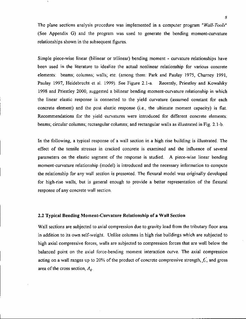
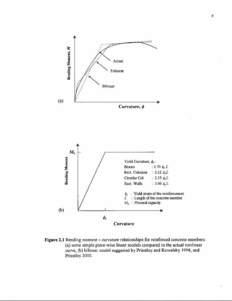
Simple piece-wise linear (bilinear or trilinear) bending moment - curvature relationships have
been used in the literature to idealize the actual nonlinear relationship for various concrete
elements', beams; columns; walls; etc. (among them: Park and Paulay 1975, Charney 1991,
Paulay 1997, Heidebrecht et al. 1999). See Figure 2.1-a. Recently, Priestley and Kowalsky
1998 and Priestley 2000, suggested a bilinear bending moment-curvature relationship in which
the linear elastic response is connected to the yield curvature (assumed constant for each
concrete element) and the post elastic response (i.e., the ultimate moment capacity) is flat.
Recommendations for the yield curvatures were introduced for different concrete elements:
beams; circular columns; rectangular columns; and rectangular walls as illustrated in Fig. 2.1-b.
In the following, a typical response of a wall section in a high rise building is illustrated. The
effect of the tensile stresses in cracked concrete is examined and the influence of several
parameters on the elastic segment of the response is studied. A piece-wise linear bending
moment-curvature relationship (model) is introduced and the necessary information to compute
the relationship for any wall section is presented. The flexural model was originally developed
for high-rise walls, but is general enough to provide a better representation of the flexural
response of any concrete wall section.
2.2 Typical Bending Moment-Curvature Relationship of a Wall Section
Wall sections are subjected to axial compression due to gravity load from the tributary floor area
in addition to its own self-weight. Unlike columns in high rise buildings which are subjected to
high axial compressive forces, walls are subjected to compression forces that are well below the
balanced point on the axial force-bending moment interaction curve. The axial compression
acting on a wall ranges up to 20% of the product of concrete compressive strength, fc, and gross
area of the cross section, Ag.
9
A
Curvature, <p
<t>y
Yield Curvature, <j>y: Beams Rect. Columns Circular Col. Rect. Walls
1.70 Sy L 2.12 SyL 2.35 SyL 2.00 SyL
Sy : Yield strain of the reinforcement L : Length of the concrete member M„ : Flexural capacity
Curvature
Figure 2.1 Bending moment - curvature relationships for reinforced concrete members: (a) some simple piece-wise linear models compared to the actual nonlinear curve, (b) bilinear model suggested by Priestley and Kowalsky 1998, and Priestley 2000.

10
Figure 2.2 depicts a typical bending moment-curvature relationship for a wall section in a high-
rise building subjected to monotonic loading. When the bending moment is applied to the
concrete wall section, the initial response is the linear elastic with the flexural stiffness (rigidity)
equal to the well known gross section property of EJg. As the bending moment increases
beyond the initial elastic range, first cracking occurs and the flexural stiffness reduces by further
growth of the first crack and initiation of additional cracks. The slope of this phase of the
response was found to be approximately parallel to the well known flexural stiffness of the
cracked transformed section EcIcr (where Icr is the cracked transformed section moment of
inertia) for typical wall sections. Low axial compression in the wall section and therefore linear
concrete stresses along the wall section at this stage of loading is the reason (i.e., concrete
compressive stresses are predominantly linear in the cracked-elastic phase of loading). Further
increase of the applied moment results in yielding of the reinforcement and hence reaching the
ultimate capacity of the under-reinforced concrete section.
The bilinear bending moment curvature model suggested by Priestley and Kowalsky 1998, and
Priestley 2000, is compared with the predicted relationship for the rectangular wall section in
Figure 2.3-a and for a bridge column (pier) section in Figure 2.3-b. While the suggested bilinear
model is reasonable for the bridge column section, the model does not provide a good
representation of the elastic deformation of the wall section.
A combination of high initial stiffness of the wall response and light amount of the vertical
reinforcement (often in high-rise buildings) makes the predicted bending moment-curvature
response fairly trilinear and therefore, it is inappropriate to use a bilinear model connecting to the
yield curvature for wall sections in high-rise buildings. In other words, the elastic linear stiffness
of the wall response is not properly captured if estimated as the capacity of the wall section
divided by the yield curvature.
2.3 - Tensile Stresses of Cracked Concrete
When concrete cracks, all the tension stresses are carried by the steel reinforcement at the
cracked sections. Between cracks and due to bond between the concrete and steel, some tensile
stresses are transferred from steel to the surrounding concrete. As a result, reinforcement
stresses are less between cracks than its maximum values at the crack, and clearly the concrete

11
Curvature, <j>
Figure 2.2 Typical bending moment - curvature relationship for a wall section in a high-rise building.

Figure 2.3 Bending moment - curvature relationships for: (a) a typical rectangular wall in a high-rise building, (b) a typical bridge pier.

13
stiffness (rigidity) is greater between cracks than at the crack itself (Figure 2.4), a phenomenon
known as tension-stiffening.
A fundamental approach to account for the tension stiffening effect is to use the average stress-
average strain relationship for concrete in tension (Vecchio and Collins, 1986). The average
strain is less than the maximum strain at a crack, and since the capacity of reinforced concrete
member is limited by the capacity of reinforcement at a crack where there are no tensile stresses,
a separate crack check calculation is necessary to determine the capacity of reinforced concrete
member whenever an average stress-average strain formulation is used.
An experimental investigation conducted at The University of British Columbia (Fronteddu and
Adebar 1992) involved tests on a series of 1.50 m long elements with 8-20M reinforcing bars
and varying cross-sectional dimensions to study the tension stiffening characteristics of concrete
under monotonic and reverse cyclic axial load. The test specimens may be considered full-scale
elements from a portion of a concrete wall. The elements were subjected to known values of
axial tension, and the resulting average tensile strains were measured. The force resisted by the
reinforcement was calculated from the measured strain and the bare bar stress-strain relationship.
This force was subtracted from the total force to determine the force resisted by the concrete in
tension. The average concrete stress at a particular strain level was determined by dividing the
calculated concrete force by the concrete cross-sectional area. Comprehensive study and analysis
of the test results can be found in Fronteddu, 1993.
Figure 2.5-a shows an example average stress-average strain relationship for concrete in tension
determined by the above-described procedure for an element subjected to monotonic tension.
When the crack first formed during the test, there was only a small reduction in the average
concrete tensile stress over the entire length of the element. As additional cracks developed, the
average concrete tensile stresses reduced further, however, even after the concrete was severely
cracked, the average concrete tension stress (the tension stiffening effect) did not completely
disappear.
Fig. 2.5-b shows an average stress-average strain relationship for concrete in tension determined
from an element subjected to cyclic loading. The envelope of the cyclic average stress-average
strain relationship is very similar to the monotonic relationship. Unloading and reloading of the

14
Segment of a wall Concrete tensile Steel stress Concrete flexural stress distribution distribution stiffness (rigidity)
distribution in the elastic range
Figure 2.4 Tension stiffening effect of a cracked reinforced concrete wall element.
15
concrete specimen followed a reduced slope (i.e., softer path) than the initial slope (concrete
modulus of elasticity in this case). The unloading and reloading slope continues to reduce further
as the concrete is subjected to higher strain. Fig. 2.5-c shows a simplified model for the average
stress-average strain relationship for concrete under cyclic tension, where the small residual
strains under zero stress are ignored for simplicity. Prior to cracking, concrete is an elastic
material. After cracking, the unloading and reloading path, i.e., the slope of the average stress-
average strain relationship, depends on the maximum tensile strain previously reached. A similar
model for the average stress-average strain relationship has been suggested by Vecchio 1999.
2.4 Bending Moment-Curvature Response Under Monotonic Loading
The monotonic average stress-average strain relationship for concrete in tension (Figure 2.5-a) is
combined with the stress-strain relationship for concrete in compression and the stress-strain
relationship for reinforcement (illustrated in Appendix A) to develop the relationship between
the applied bending moment and the curvature for a typical wall section subjected to a variety of
applied axial compression and amount of vertical reinforcement (see Figure 2.6).
As mentioned earlier, the slope of the initial portion of the relationship depends only on the
concrete geometry and is equal to EJg.. The extent of the initial linear response depends on the
concrete tensile strength and the axial compression acting on the wall. Increasing the applied
axial compression increases the wall flexural capacity and extends the initial linear elastic
response of the wall section (Fig. 2.6-a). The secondary slope of the bending moment-curvature
relationship depends on the concrete geometry and the amount of the vertical reinforcement and
is approximately equal to the flexural stiffness of the cracked transformed section, EJcr.
Increasing the amount of the vertical reinforcement in the tension side of the wall section
increases the secondary slope of the bending moment-curvature relationship as well as the
flexural capacity of the section (see Fig. 2.6-b). The point at which the bending moment-
curvature relationship becomes nonlinear does not change significantly with increasing the
reinforcement amount.

Figure 2.5 Response of concrete in tension (experimental results from Fronteddu, 1993): (a) monotonic loading (predicted and observed), (b) cyclic loading, (c) proposed model for cyclic loading.

17
0.6 0.8 1
Curvature (rad/km)
p f = 3.0%
yP f =2.0%
p f = 1.0%
p f = 0.5%
6.0 m < 6*4
TJ- P=0.1 f c A a •
i i _ 4 : pf— \
p w = 0.25%
0.4 06 0.8 1
Curvature (rad/km)
Figure 2.6 Bending moment-curvature relationships for typical concrete walls subjected to monotonic loading: (a) influence of axial compression, (b) influence of reinforcement.

18
2.5 Bending Moment-Curvature Response under Cyclic Loading
Figure 2.7-a shows the bending moment-curvature response of a typical wall section subjected to
increasing cycles of bending. The wall response during any one cycle of loading depends on
how far the wall was loaded in the previous cycle. Therefore, the tensile strain at each layer
along the wall was recorded for each load cycle. As the tensile strain for a particular load cycle
varies at each concrete layer, the average stress-average strain relationship varies at each layer
according to the relationship shown in Fig. 2.5-c.
The different average tensile stress-average tensile strain relationships recorded in each load
cycle and used in the prediction of the consecutive cycle are shown in Fig. 2.7-b. These
relationships are shown and labeled only for the outer layer of the wall section. Interior wall
layers (next to the outer fiber) have experienced less tensile strain in the previous cycle and
therefore have more tensile stress. This is depicted by the dotted lines on the average stress-
average strain relationship for each load cycle.
Figure 2.7 indicates that during an earthquake motion, a wall section would experience a
response that is bounded by two extremes, a "previously uncracked" section response in which
there are significant concrete tensile stresses, and a "severely cracked" section response in which
there are very little residual concrete tensile stresses. The severely cracked response is different
than the response predicted by completely ignoring the concrete tensile stresses (Fig. 2.7-b, label
D and E).
The change of section response due to extensive cracking during the earthquake motion degrades
the flexural stiffness of a wall building and as a result, lengthens the building period, a well
known effect long recognized in the literature (e.g., Paulay and Priestley, 1992). More elaborate
discussion follows in Chapter 4.
Note that in making the prediction of the bending moment-curvature relationships shown in
Figure 2.7-a, only the influence of cyclic loading on degrading the tensile stresses of concrete
was considered. Cyclic response of concrete in compression and of the reinforcement are known
to result in residual strains at zero load upon reloading to an increased deformations. An
investigation carried out (in Appendix B) on a typical wall section showed that the residual
strains are small and the resulting relationships are only slightly offset from the origin and
therefore these can be ignored without significantly affecting the results,
discussed further in Chapter 3, Section 3.8.
19
This assumption is
2.6 Trilinear Bending Moment-Curvature Relationship for Concrete Walls
It is proposed that the bending moment-curvature response of a wall section including the effect
of axial compression acting on the wall, the amount of vertical reinforcement and the state of
cracking (i.e., tension stiffening effect) can be represented by a simple trilinear relationship.
The trilinear relationship that represents the stiffest response that the wall would experience if
loaded monotonically to failure without having been previously cracked (i.e., previously
uncracked response) is termed upper-bound response. The trilinear relationship that represents
what is observed when the wall is reloaded after being severely damaged from a previous load
cycle (i.e., severely cracked response) is termed lower-bound response (See Figure 2.8).
Both the upper-bound and lower-bound trilinear relationships are defined by four parameters: the
slope of the elastic linear response (first linear segment) EJg , the slope of the second linear
segment (secondary slope), EcIcr, the bending moment defining the intersection of the first and
second linear segments, Mi, and the flexural capacity M„. In the following, each of the four
parameters is described further and a method to determine each parameter is presented.
2.6.1 Slope of the Linear Elastic Response, EJg
The gross moment of inertia, Ig, is easily determined by hand calculations for typical wall
sections. The gross concrete geometry is normally used as the effect of typical reinforcement
amount is negligible.
The modulus of elasticity of concrete, Ec, has several definitions and several formulae in the
literature. The secant modulus of elasticity at a stress of 0.4 fc is adopted in this thesis and the
expression used is the one adopted by CSA Standard A23.3-94.
[2.1]

20
120000
Figure 2.7 Predicted influence of cyclic loading on: (a) bending moment - curvature relationship of a typical concrete wall, (b) the tension stress-strain relationship for the most highly strained concrete in the wall.
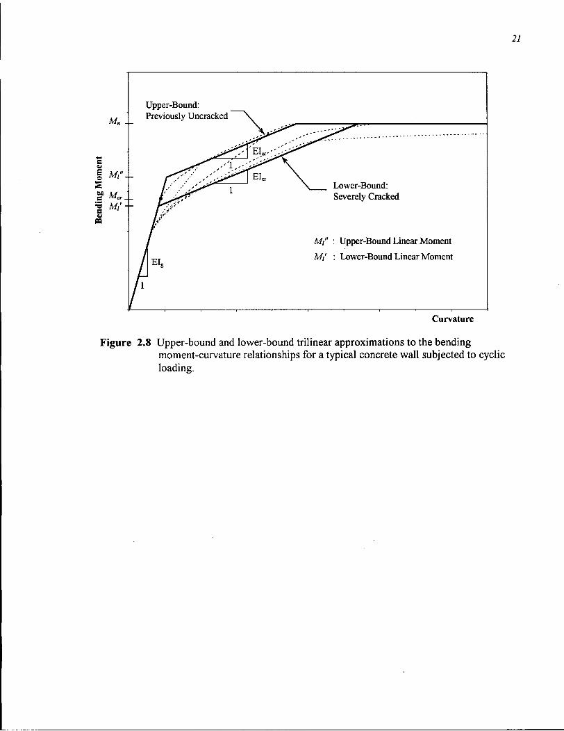
21
Upper-Bound:
Curvature
Figure 2.8 Upper-bound and lower-bound trilinear approximations to the bending moment-curvature relationships for a typical concrete wall subjected to cyclic loading.

22
Where Ec is the modulus of elasticity in MPa, yc is the mass density of concrete in kg/m3, and fc
is the specified compressive strength in MPa. For normal density concrete (yc = 2400 kg/ m3),
having a compressive strength less than 40 MPa, the following expression can be also used.
2.6.2 Slope of the Second Linear Segment, EJcr
The secondary slope of the trilinear bending moment-curvature relationship depends primarily
on the concrete geometry and the amount of reinforcement. This slope is assumed to be equal to
the flexural stiffness of the cracked transformed section, EcIcr. The value of EcIcr for a wall
section of arbitrary shape and reinforcement arrangement can be computed using a plane section
analysis program and is equal to the initial slope of the bending moment-curvature relationship
for zero axial load and no tensile stresses in the concrete.
The cracked section moment of inertia, Icr, can easily be calculated for a rectangular section with
concentrated tension reinforcement. Complex wall geometry with distributed vertical
reinforcement makes the calculation of Icr difficult. Appendix C illustrates the detailed
calculation of Icr for a general flanged wall section.
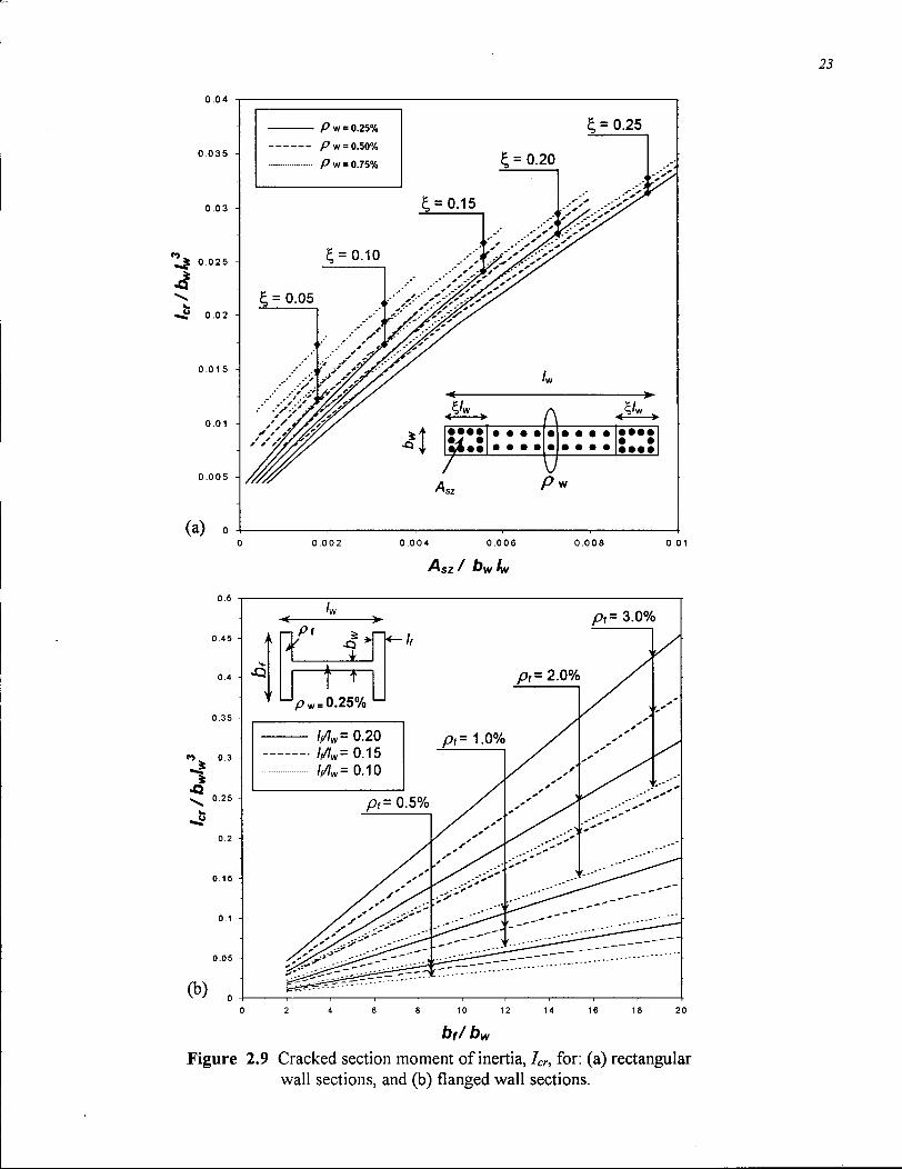
Figure 2.9 is a design chart that can be used to determine Icr for rectangular and flanged wall
sections. Program "Wall-Tools" was used to generate the data for the chart.
For rectangular walls (Fig. 2.9-a), the reinforcement area in the boundary zone and in the web,
and the length of the concentrated boundary zone are required to determine the value of Icr.
Figure 2.9-a may also be used for a T-shaped wall in which the flange is on the tension side. The
reinforcement in the tension flange is considered as the area of reinforcement in the boundary
zone, Asz..
For flanged walls (Fig 2.9-b), the geometry of the compression flange (width, bf, and thickness,
//), the reinforcement in the tension flange expressed as a ratio of the concrete area, py, and the
web geometry (length, lw, and width bw) are needed to determine the value of Icr- Although the
data for Icr plotted in Fig. 2.9-b was obtained for symmetrical flanged wall sections, the value of
[2.2]
23
0.04
0.035
0.03
0.025
«J? 0.02
0.015 H
(a)
P W = 0.25%
P w = 0.50%
P w = 0.75%
£ = 0.25
g, = 0.20
0 0.002 0.004 0.006 0.008 0.01
Asz / b\f/ lw
r> 0.3
•G ^ 0.25
(b)
* i
pf= 3.0%
t U p w = 0.25% pf=2.0%
= 0.20 Ww = = 0.15 ///w = = 0.10
p,= 1.0%
pf= 0.5%
6 f / 6 W
Figure 2.9 Cracked section moment of inertia, Icr, for: (a) rectangular wall sections, and (b) flanged wall sections.

24
Icr may be approximated for unsymmetrical flanged wall sections by using the geometry of the
compression flange to determine bfl bw and /// lw and calculate pf from the area of reinforcement
in the tension flange divided by the area of the compression flange.
2.6.3 Flexural Capacity, M„
As mentioned, the flexural capacity of an under-reinforced wall section is limited by yielding of
the reinforcement at a crack where no tensile stresses exist in the concrete. The flexural capacity
can be determined as the maximum bending moment in the bending moment-curvature response.
Alternatively, the ultimate compression strain scu, and the stress block factors ocj and Bj can be
used to determine the strain distribution and the stress resultant along the wall section. This well
known procedure is summarized in Fig. 2.10 for completeness. Since an accurate estimate of the
flexural capacity is required to determine the corresponding maximum seismic shear, the
longitudinal web reinforcement should be accounted for when computing the flexural capacity of
a wall section as illustrated in Fig. 2.10.
2.6.4 Linear Bending Moment, Mi
The linear bending moment, Mi, is the bending moment that defines the transition from the
primary slope EJg (first linear segment) to the secondary slope EJcr (second linear segment) of
the trilinear bending moment-curvature relationship. This bending moment is influenced by the
amount of axial compression acting on the wall and the tension stiffening effect of concrete. A
rigorous approach to determine the Mi value is to define a trilinear bending moment-curvature
relationship (with the other three parameters previously defined) that has the same area under the
curve as the actual nonlinear bending moment-curvature relationship. This approach requires the
determination of the actual nonlinear bending moment-curvature relationship using plane
sections analysis. Integrating the area under the actual nonlinear relationship and making it
equal to the area under the trilinear relationship gives a quadratic equation for Mi. Solution of
this equation is shown in Appendix D.

(I) Assume depth of neutral axis, C, & a = fr.C
fy — fsi E s . £ s j ^ -fy
(III) C c = a, fc' a b
(IV) If : C 0 + Z A5 C fsi = P
Then : H , = C c [ C - a/2] + P (\J2 - C) + Z f5i (C - x;)
Else : Repeat from Step (I)
Where: (from CSA-A23.3-94) 8CU=0.0035; a, = 0.85 -0.0015 fc'> 0.67; 0,= 0.97 - 0.0025 fc' > 0.67
Figure 2.10 Procedure to determine the flexural capacity, M„, of a typical wall section.

26
A trilinear bending moment-curvature relationship that has the same area under the curve as the
actual nonlinear relationship makes the rotation of a wall segment along the height of the
building being similar whether computed by the actual nonlinear relationship or the trilinear
relationship. Further discussion and use of this concept is illustrated in Chapter 5.
The approach of equal area under both the nonlinear and trilinear curves can be used to
determine the value of Mi for both the upper-bound and lower-bound responses. The linear
bending moment for upper-bound response, designated as Mi, is obtained when integrating the
area under the actual nonlinear upper-bound response (i.e., previously uncracked section with
monotonic tensile stresses in concrete; envelope of Fig. 2.7-a). The linear bending moment for
lower-bound response, designated as Mi, is obtained when integrating the area under the actual
nonlinear lower-bound response (i.e., severely cracked section with little tensile stresses; Fig 2.7-
a case D). Since the maximum tensile strains reached in the previous load history are not known,
the average tensile stress-average tensile strain relationship is not uniquely defined. Therefore,
the actual nonlinear bending moment-curvature relationship that is calculated by completely
ignoring the concrete tensile stresses (Fig. 2.7-a case E) is modified to account for some residual
tensile stresses in the concrete and used for the integration procedure. The actual nonlinear
bending moment-curvature relationship with zero tensile stress is modified so that the fairly
rounded part of the curve is ignored and the somewhat linear secondary slope is extended to
intersect the ultimate flexural capacity Mn (see Fig. 2.8). It is interesting to note that the linear
bending moments (Mi and M; ) are different from the first cracking moment, Mcr, as shown in
Fig. 2.8.
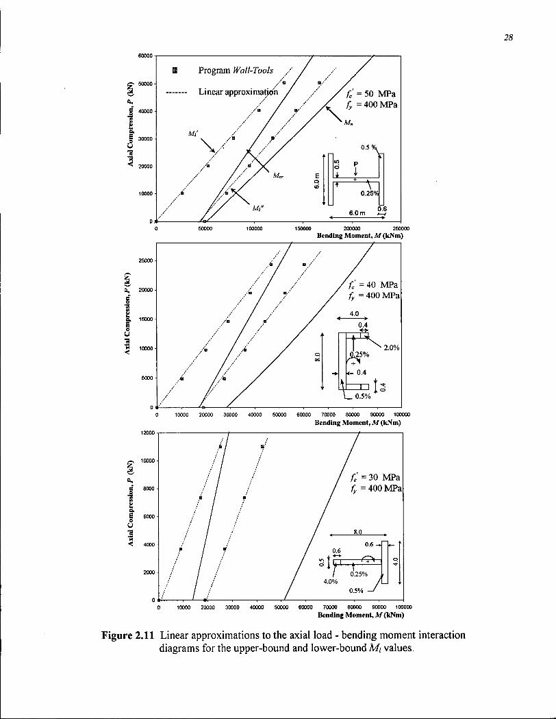
The rigorous method just described for determining Mi was incorporated in program "Wall-
Tools" and the program was used to generate the data for different wall sections as shown in Fig.
2.11. For each wall section with certain material properties and given axial compression, "Wall-
Tools" computes EJg, EcIcr and M„\ determines the actual nonlinear moment-curvature
relationship; integrates the area under the nonlinear relationship; and finally determines the best-
fit value of Mi (that gives the same area under both relationships). Each wall section was run for
a variety of axial compression values and the results of the linear bending moment (both upper-
bound and lower-bound) are plotted in Fig 2.11.

27
The results in Figure 2.11 show that M/ is approximately a linear function of the axial
compression (similar to the well-known axial compression-bending moment interaction
relationship for under-reinforced sections) and that both upper and lower-bound linear bending
moment have nearly the same slope. The influence of tension stiffening on the predicted linear
bending moment is transparent in the difference between the upper and lower-bound responses,
and can be approximated as a linear relationship as well. Hence, to develop a simple relationship
to determine the linear bending moment, Mi, the following expression was used:
M,=C,.P + C0.f [2.3] / 1 2J cr
Where, P is the compression force acting on the wall, fcr, the cracking strength of concrete
defined conservatively as 0.33 (fc )v\ and Cy and C2 are linear coefficients.
The previous expression resembles the cracking moment, Mcr, linear equation:
"cr^j-V + W-fcr [ 2 A ]
g
In which, Ag is the gross concrete area of the wall section, and S is the section modulus (Ig/y) to
the tension side of the wall. Thus, the linear bending moment function can be simply expressed
as the cracking moment equation with two additional parameters a, and B, to consider the
difference in the Mi values from the cracking moment:
Ml = a . ( - p ) . P + p.(5)./ c r [2.5] g
As shown in Figure 2.11, the slope of the linear bending moment (as function of P) was nearly
equal for both the upper and lower bound Mi and thus a, would be the same for both Mi and Mi.
The intercept of the lower-bound linear bending moment function, Mi, was equal to zero as the
cracking strength, fcr, was ignored. Therefore, the cracking strength, fcr, may be taken equal to
zero or alternatively, B - 0.0 and the second term in the above equation drops out when
determining the lower-bound response, Mi.
28
Program Wall-Tools
Linear approximation fc = 50 MPa fy =400 MPa
Mi' 0.5 %
V p
0.25%|
6.0 m 0.6
50000 100000 150000 200000 250000
Bending Moment, M (kNm)
0 10000 20000 30000 40000 50000 60000 70000 80000 90000 100000
Bending Moment, M (kNm)
fc = 30 MPa fy = 400 MPa
8.0
0.6 -J
r - t -/ 0.25°/
4.0%
0.5%
10000 20000 30000 40000 50000 6X00 70000 80000 90000 100000
Bending Moment, M (kNm)
Figure 2.11 Linear approximations to the axial load - bending moment interaction diagrams for the upper-bound and lower-bound Mi values.

29
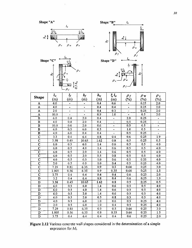
To estimate the parameters a, and B(for upper-bound only), program "Wall-Tools" was used to
determine Mi, using the rigorous method, for numerous wall sections with various concrete
geometry and reinforcement amount and arrangement (Fig. 2.12). Each wall section was run for
the corresponding Ec and fcr). In each analysis, both the upper and lower bound Mi was
determined for a range of axial compression on the wall.
Data points obtained for Mi for the different axial compression levels in each analysis were fitted
to a straight line using the least squares method. The slope of the fitted Mi linear function
divided by the slope of the cracking moment function (S/Ag) gives the parameter a, and the
intercept of the fitted linear function divided by the cracking moment at zero axial compression
(Sfcr) determines the parameter /?.
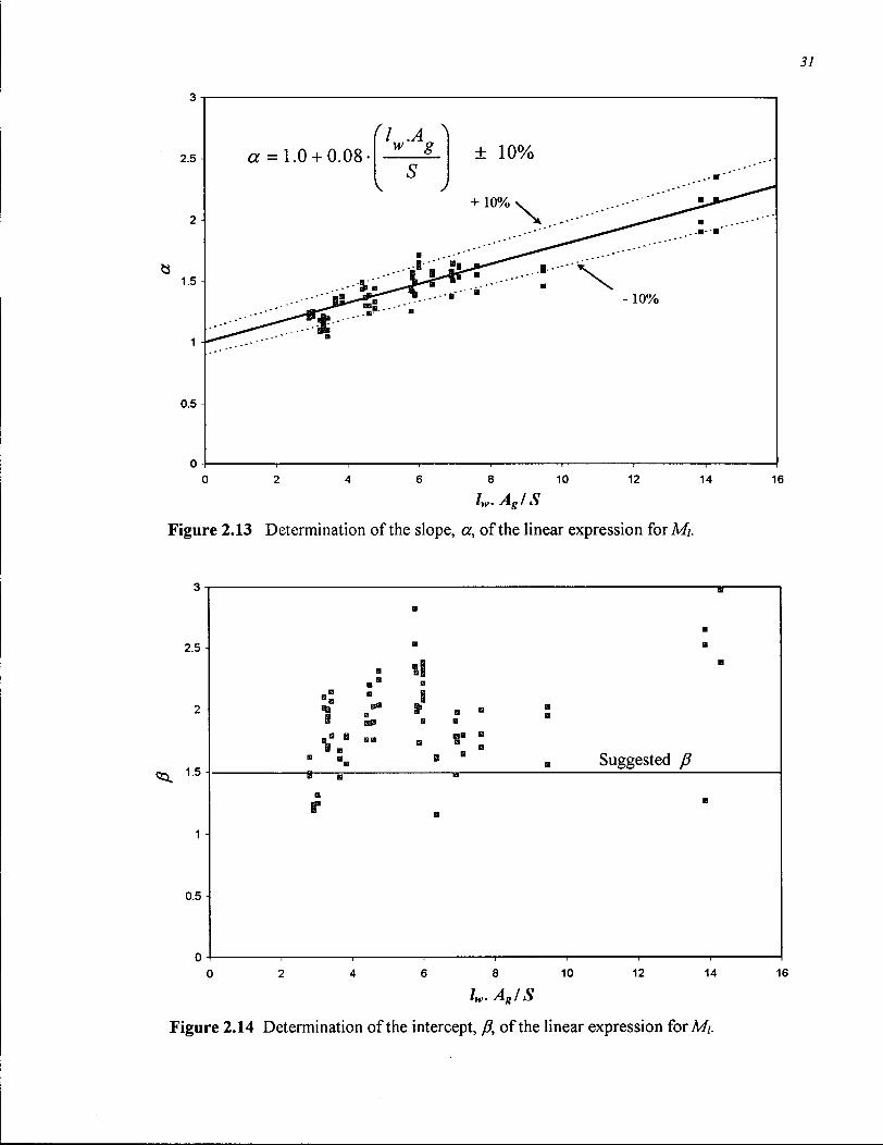
Figures 2.13 and 2.14 show the variation of the parameters a, and B, plotted against the
geometrical properties of the wall sections. Figure 2.13 indicates that the trend of the parameter
a, can be approximated by the following expression:
where /„,, is the length of the wall section.
Figure 2.14 shows the scatter of the data for the parameter B with respect to the geometry of the
wall section (note that B = 0.0 for the lower-bound predictions and the data shown are only for
the upper-bound linear bending moment). Despite the large scatter of /? values (ranging from
approximately 1.0 to 3.0), it has little effect on the predicted Mi value for the upper bound
response, particularly if the wall is subjected to a relatively high axial compression. A B of 1.5 is
suggested for the upper-bound Mi value (Mi ).
Incorporating Equations [2.5] and [2.6] and the suggested values of /?, a simple relationship to
determine Mi is as follows:
different material properties (concrete compressive strength fc ranging from 30 to 60 MPa, and
a = 1.0 + 0.08- [2.6]
m, = p.f + — s + ompi w
[2.7]
Shape "A" Shape "B"
Pz Pw Pi
Shape "C"
Shape lw
(m) k
(m) bf
(m) bw
(m) £ L (m)
Pf (%)
Pw (%)
Pz (%)
A 6.0 - - 0.4 0.6 - 0.25 2.0
A 4.0 - - 0.4 0.4 - 0.25 2.0
A 2.0 - - 0.4 0.3 - 0.25 2.0
A 10.0 - - 0.9 1.0 - 0.5 3.0
B 6.0 0.4 2.0 0.4 - 2.0 0.25 -B 4.0 0.4 2.0 0.4 - 0.5 0.25 -B 10.0 0.6 2.0 0.6 - 0.5 0.5 -B 6.0 0.5 6.0 0.5 - 1.0 0.5 -B 4.0 6.0 0.4 0.4 - 0.5 0.25 -C 3.2 0.4 6.4 0.8 0.4 0.6 0.25 1.9
C 3.58 0.45 10.65 1.62 0.8 0.5 0.25 0.5
C 6.0 0.5 6.0 1.4 0.6 0.5 0.5 4.0
C 6.0 0.5 4.0 1.4 0.6 0.5 0.5 4.0
C 6.0 0.5 2.0 1.4 0.6 0.5 0.5 4.0
C 6.0 0.5 2.0 0.5 0.8 0.5 0.5 4.0
C 4.0 0.5 6.0 1.0 0.6 0.5 0.25 4.0
C 2.0 0.5 6.0 1.0 0.4 0.5 0.25 4.0
C 7.29 0.81 6.35 0.9 0.5 0.64 0.25 3.0
C 1.905 0.56 6.35 0.9 0.35 0.64 0.25 1.5
C 3.75 0.4 6.4 0.4 0.4 0.6 0.25 2.0
D 3.2 0.4 6.4 0.8 0.4 0.6 0.25 1.9
D 3.58 0.45 10.65 1.62 0.8 0.5 0.25 0.5
D 6.0 0.5 6.0 1.4 0.6 0.5 0.5 4.0
D 6.0 0.5 4.0 1.4 0.6 0.5 0.5 4.0
D 6.0 0.5 2.0 1.4 0.6 0.5 0.5 4.0
D 6.0 0.5 2.0 0.5 0.8 0.5 0.5 4.0
D 4.0 0.5 6.0 1.0 0.6 0.5 0.25 4.0
D 2.0 0.5 6.0 1.0 0.4 0.5 0.25 4.0
D 7.29 0.81 6.35 0.9 0.5 0.64 0.25 3.0
D 1.905 0.56 6.35 0.9 0.35 0.64 0.25 1.5
D 3.75 0.4 6.4 0.4 0.4 0.6 0.25 2.0
Figure 2.12 Various concrete wall shapes considered in the determination of a simple expression for Mi.
31
2.5
1.5
0.5
(I .A > a = 1.0 + 0.08- W 8
S V J
± 10%
+ io% •
B
- 10%
Figure 2.13 Determination of the slope, a, of the linear expression for Mi.
10 12 14 16
2.5
1.5 A
0.5
Suggested B
ly\" Ag I S 10 12 14 16
Figure 2.14 Determination of the intercept, /?, of the linear expression forM/.

32
where, >t?= 1.5 for the upper-bound response, and /?= 0 for the lower-bound response. Equation
[2.7] is used to determine Mi in an approximate way in lieu of the more rigorous method (equal
area under the curve method) described earlier. Figure 2.15 compares the results from Equation
[2.7] with the results of Mi determined using the rigorous method. A reasonable agreement is
found.
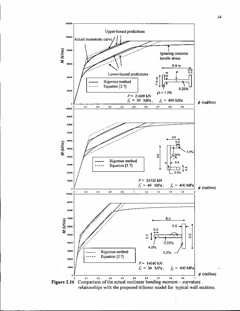
Figure 2.16 shows the actual nonlinear upper-bound and lower-bound bending moment-
curvature relationships for a selection of wall sections. Idealized trilinear models determined
using both the rigorous method and Equation [2.7] for both the upper and lower-bound are also
shown for comparison. A reasonable accuracy (within approximately +10%) is found as
previously shown in Figure 2.15.
2.7 Concluding Remarks
A study of the response of wall sections with high initial stiffness and light amounts of vertical
reinforcement (typical in most high rise walls) indicated that the uncracked portion of the
bending moment-curvature response is very significant and therefore, the elastic deformations of
the response are not appropriately represented by other simpler models that tend to ignore the
uncracked stiffness.
A trilinear bending moment-curvature relationship (nonlinear flexural stiffness), that captured
the effect of cracking, was proposed for concrete walls in high rise buildings and the parameters
needed to determine the model were presented. While the largest advantage of the proposed
relationship over other simpler models occurs with high rise walls, the proposed model is
applicable to all concrete walls.
Calibration of the proposed trilinear bending moment-curvature relationship against test results
from a large-scale slender concrete wall is illustrated in the next chapter.

33
Mi, rigorous method
Figure 2.15 Comparison of Mi determined using the simple expression (Eq. [2.7]) with the value determined using the more rigorous method.
34
Upper-bound predictions
Actual monotonic curve/
Ignoring concrete tensile stress
6.0 m 0.6
Lower-bound predictions Rigorous method Equation [2.7]
fit L
0.25% p (= 1.0%
P = 21600 kN fc = 50 MPa, fy = 400MPa ^ (rad/km)
0.1 0 2 0.3 0.4 0.5 0.6 0.7 0.8
4.0 0.4
Rigorous method Equation [2.7]
| ^ 2.0% , 0.25%
0.4
\ _ 0.5%
P = 24320 kN fc = 40 MPa, fy = 400 MPa ^ (rad/km)
0.2 0.4 0.6 0.8 1.2 1.4
8.0
0.6 o
0.6 •
Rigorous method Equation [2.7]
4.0% 0.25%
0.5%
P= 14640 kN fc' = 30 MPa, fy = 400MPa
<j> (rad/km) 0.1 0.2 0.3 0.4 0.5 0.6 0.7 0.8
Figure 2.16 Comparison of the actual nonlinear bending moment - curvature relationships with the proposed trilinear model for typical wall sections.
Chapter 3
Experimental Study of a Large-Scale Slender Wall
3.1 General
In order to validate the trilinear bending moment-curvature model developed in Chapter 2, an
experimental investigation was carried out on a tall slender wall where the response is dominated
by flexural deformations. The experimental study was done jointly with Bryson (2000) who was
responsible for the design and construction of the test specimen. The instrumentation and testing
procedure was done jointly, while the analysis of the test results was done entirely as part of this
thesis. In this chapter a brief overview of the experimental program is given and the results that
are relevant to the analytical developments in this thesis are presented. A complete report on the
test is given by Adebar, Ibrahim and Bryson (2000).
Several researchers and numerous studies have been conducted to measure different aspects of
concrete wall response. Abrams (1991) listed 44 references for the measured response of
concrete walls. Thomsen and Wallace (1995) summarized the work to date. To the author's
knowledge, none of these studies involved a wall that was as slender as the wall tested in this
study and none were conducted on such a large-scale specimen.
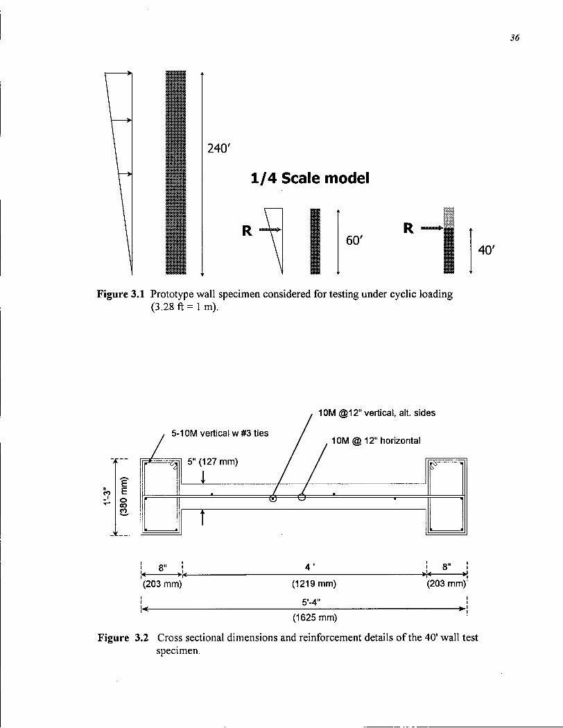
3.2 Description of Test Specimen
The prototype wall was assumed to be 240 ft high and to have a length of 22 ft. A 1/4 scale
model of the prototype wall (i.e., a 60 ft high wall) was considered for testing under simulated
seismic loading. A triangular load distribution along the wall height simulating seismic loading
may be represented by the resultant lateral load at two-thirds of the height of the wall (i.e., 40 ft
from the base). Accordingly, a 40 ft high wall specimen was constructed for testing under single
lateral load at the top of the wall (see Figure 3.1).
The specimen was 40 ft high by 5 ft - 4 in. long with a flanged cross section. The web was 4 ft
long by 5 in. thick and the flanges were 8 in. long and 15 in. thick. The vertical reinforcement in
35
240'
1/4 Scale model
60'
36
40'
Figure 3.1 Prototype wall specimen considered for testing under cyclic loading (3.28 ft = 1 m).
co E E o oo CO
5-10M vertical w #3 ties
10M @12" vertical, alt. sides
10M @ 12" horizontal
5" (127 mm) / /
I / / —
/ 1 . • •
It t
»
i 8" (203 mm)
4' (1219 mm)
5'-4"
j 8" (203 mm)
(1625 mm)
Figure 3.2 Cross sectional dimensions and reinforcement details of the 40' wall test specimen.

37
the flange consisted of 5-10M reinforcing bars enclosed by 10M ties spaced at 2.5 in. in the
lower 10 ft of the wall and spaced at 6 in. in the remaining height of the wall. The web was
reinforced with 10M bars spaced at 12 in. vertically and horizontally. Figure 3.2 shows the
cross sectional dimensions and reinforcement details.
In most high-rise buildings there are numerous levels of parking below grade. The parking
structure is normally considerably larger than the tower and has perimeter walls that are tied to
the tower walls by the concrete slabs at each level. As a result, the critical section of the tower
walls (i.e., the potential plastic hinge region) is normally at grade level, not immediately above
the foundation as is normally the case in bridge columns. One consequence of this is that there is
much less pull-out of the vertical reinforcement from wall foundations. To simulate this effect in
the wall specimen, the critical section was located 16 in. up from the base of the wall. The wall
and the base were cast separately, and the construction joint was located at the desired critical
section. Additional vertical wall reinforcement was provided below the critical section.
Due to the limited height in the laboratory, the wall specimen was constructed and tested in the
horizontal position (see Figures 3.3 and 3.4). The wall was cast horizontally in a wooden form.
After the concrete had gained sufficient strength (approx. four weeks), the wall was removed
from the wooden form and lifted into place on top of Teflon sliding bearings located at 9'-9"
from the base of the wall and at 8'-5" from the top of the wall (see Figure 3.5). Prior to
constructing the base of the wall, a test was conducted to determine the magnitude of the lateral
force at the "top" of the wall that was required to overcome the friction in the Teflon bearings
that supported the dead weight of the wall. The lateral load required to maintain movement of
the wall was determined to be 3.65 kN which is approximately 2% of the maximum load applied
during the test. The base of the wall was cast around shear pins and bolts inserted into the
laboratory strong floor in order to minimize movement of the base during loading of the wall.
The specimen was tested after the concrete in the wall above the critical section had reached an
age of 140 days (approx. 4.5 months). At that time the cylinder compressive strength of the wall
concrete was measured to be 49 MPa.
All of the 10M reinforcing bars that were used to construct the wall came from a single heat of
reinforcing steel. Samples of the reinforcing bars were tested. Based on an assumed cross-

Figure 3.3 Large-scale slender wall test undertaken to validate the proposed trilinear model.


40
sectional area of 100 mm2, the yield strength was determined to be 455 MPa, while the ultimate
strength was found to be 650 MPa.
3.3 Test Set-up
In addition to applying a lateral load at the "top" of the wall, an axial load of 1500 kN (10% of/ c
Ag) was applied to the wall during the test. Two hydraulic actuators located below the base of
the wall applied the axial load. The actuators were used to pull down on four 1-1/4 in. diameter
Dywidag bars attached to the top of the wall (see Figures 3.3 and 3.4). The hydraulic actuators,
which were subjected to a constant pressure during the test, had sufficient stroke to allow the
required movement of the Dywidag bars during the cycling of the lateral load. To reduce the
shear force between the wall base and laboratory floor, the hydraulic actuators that applied the
axial force were reacted directly against the base of the wall (see Figure 3.4).
The lateral load was applied using an MTS hydraulic actuator with a maximum stroke capability
of +/- 12 in. The lateral load was applied at 38 ft - 7 in. from the base of the wall which
corresponds to 37 ft - 3 in. from the critical section (construction joint). The actuator was
mounted horizontally on a reaction steel column that was bolted to the lab floor and was
controlled by a wave-form generator.
3.4 Instrumentation
Instrumentation was used to measure displacements at various points on the wall, the lateral and
axial loads, and strains at various locations in the wall specimen. Figure 3.6 shows a summary
of the instrumentation used during the test.
Two LVDT's (each with +/- 6 in. stroke) were mounted at the top of the wall to verify the lateral
displacement measurements obtained from the LVDT within the hydraulic actuator. An
additional LVDT was used to measure the lateral movement of the wall at 200 in. from the base.
Axial displacement was measured at the middle of the cross section at 200 in. from the base of
the wall using an LVDT mounted to a fixed steel frame supported on the floor. Two additional
LVDT's were used to measure the longitudinal displacement over a 64 in. gage length in the

41
Figure 3.5 Teflon sliding bearings supporting the slender wall specimen tested in a horizontal position.

43
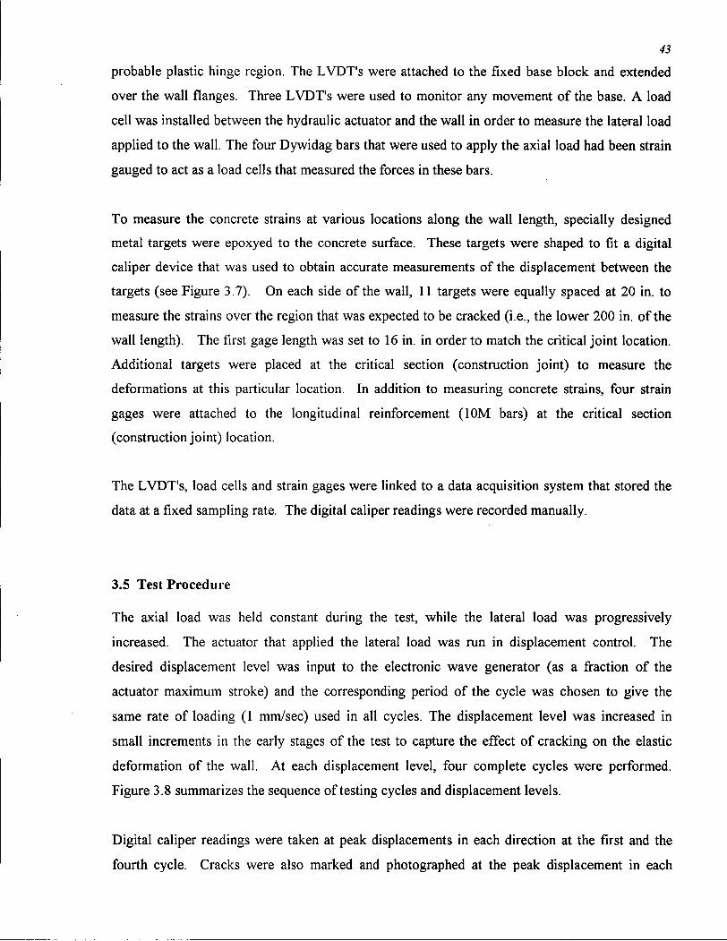
probable plastic hinge region. The LVDT's were attached to the fixed base block and extended
over the wall flanges. Three LVDT's were used to monitor any movement of the base. A load
cell was installed between the hydraulic actuator and the wall in order to measure the lateral load
applied to the wall. The four Dywidag bars that were used to apply the axial load had been strain
gauged to act as a load cells that measured the forces in these bars.
To measure the concrete strains at various locations along the wall length, specially designed
metal targets were epoxyed to the concrete surface. These targets were shaped to fit a digital
caliper device that was used to obtain accurate measurements of the displacement between the
targets (see Figure 3.7). On each side of the wall, 11 targets were equally spaced at 20 in. to
measure the strains over the region that was expected to be cracked (i.e., the lower 200 in. of the
wall length). The first gage length was set to 16 in. in order to match the critical joint location.
Additional targets were placed at the critical section (construction joint) to measure the
deformations at this particular location. In addition to measuring concrete strains, four strain
gages were attached to the longitudinal reinforcement (10M bars) at the critical section
(construction joint) location.
The LVDT's, load cells and strain gages were linked to a data acquisition system that stored the
data at a fixed sampling rate. The digital caliper readings were recorded manually.
3.5 Test Procedure
The axial load was held constant during the test, while the lateral load was progressively
increased. The actuator that applied the lateral load was run in displacement control. The
desired displacement level was input to the electronic wave generator (as a fraction of the
actuator maximum stroke) and the corresponding period of the cycle was chosen to give the
same rate of loading (1 mm/sec) used in all cycles. The displacement level was increased in
small increments in the early stages of the test to capture the effect of cracking on the elastic
deformation of the wall. At each displacement level, four complete cycles were performed.
Figure 3.8 summarizes the sequence of testing cycles and displacement levels.
Digital caliper readings were taken at peak displacements in each direction at the first and the
fourth cycle. Cracks were also marked and photographed at the peak displacement in each

Figure 3.7 Measuring concrete strains at various locations along the wall height: (a) metal targets epoxyed to concrete, (b) digital caliper device.

45
46
direction at the first and fourth cycle. Readings from the LVDT's, strain gages, and load cells
readings were recorded continuously by the data acquisition system at a sampling rate of 5
readings/sec.
3.6 Corrections to Measured Results
Figure 3.9 summarizes the measured (uncorrected) load-displacement relationship of the wall.
Due to a problem with the data acquisition system, the test data for the 30 and 45 mm
displacement cycles were not recorded. Therefore additional cycles to +/- 48 mm displacement
levels were added.
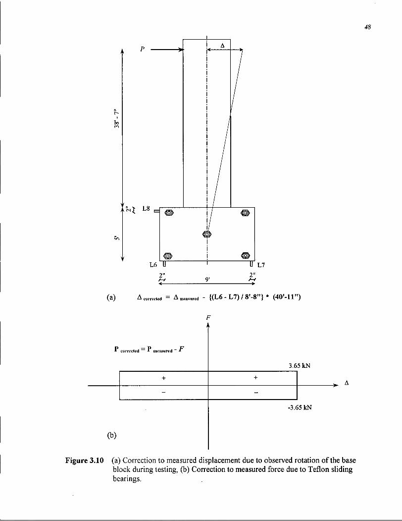
During the test it was observed that the base of the wall did rotate somewhat. The measured
displacement of the base was used to estimate the rigid body motion at the top of the wall, and
the recorded displacement of the top of the wall was corrected to account for this effect. To
estimate the displacement of the wall top due to rotation of the wall base, the center of rotation
was assumed be at the middle bolt in the base (see Fig. 3.10-a). Displacement readings of LVDT
6 and 7 were used to compute the rigid body rotation of the base at any instant. The rotation of
the base multiplied by the distance from the middle bolt to the location where the lateral
displacement was measured at the "top" of the wall (11823 mm) gives the displacement that
should be subtracted form the recorded data. Note that the base rotation times the short vertical
distance from the middle bolt to LVDT 8 (711 mm), gives an estimate of the displacement
readings of L8 if the center of rotation was at the center of the block as assumed. Several such
checks were made and good correlation was found.
The lateral load was corrected for the friction force due to the Teflon bearings that supported the
dead weight of the wall. The friction force for one complete cycle of loading was assumed to
follow Coulomb friction model as shown in Fig 3.10-b. These forces were subtracted from the
load recorded for each and every cycle. The corrected load-displacement relationship including
the effect of base rotation and friction is shown in Figure 3.11.

F
p
i
corrected P measured ~ F
3.65 kN
+ +
- -
(b)
-3.65 kN
Figure 3.10 (a) Correction to measured displacement due to observed rotation of the base block during testing, (b) Correction to measured force due to Teflon sliding bearings.

49
3.7 Summary of Test Observations
As expected, flexural behavior dominated the response of the slender wall specimen. No early
strength decay caused by lack of shear capacity or bond failure was observed. Significant
diagonal cracking (flexure-shear cracking) was observed near the later stages of the test,
however, these cracks did not appear to influence the overall response of the wall.
According to the strain gauge readings, first yielding of the longitudinal reinforcement occurred
at the critical section at a lateral displacement of 48 mm.
Spalling of the cover at the critical joint location occurred at a displacement level of 200 mm and
some metal targets were lost. To fail the specimen, further cycling was undertaken and the
longitudinal reinforcement buckled at the critical section. Two longitudinal reinforcing bars were
observed to have fractured.
3.8 Discussion of Test Results
As shown in Figure 3.11, the hysteresis loops reached the monotonic load capacity showing no
strength decay within a realistic range of deformations. Strain hardening of the reinforcement in
the post-yield deformation caused additional gain in strength (over-strength). This feature of
stable hysteresis loops is typical of flexural dominant response.
The initial slope of the load-displacement response was essentially unchanged, even after cycling
the specimen further into the inelastic deformation range, the initial slope remained close to the
initial uncracked gross stiffness. Upon unloading from one direction and reloading in the other,
the stiffness increased as the load approached zero. As the moment reduced, the axial
compression closed the cracks and the wall responded nearly as an uncracked wall.
The small residual displacement at zero load and small residual load at zero displacement
supported the inherent assumption in the trilinear bending moment-curvature model that the
initial portion of any loading cycle will pass through the origin and follow the original uncracked
response up until exceeding the lower-bound Mi, as discussed in Chapter 2, Section 2.5. (See
also Chapter 5, Section 5.4.1).
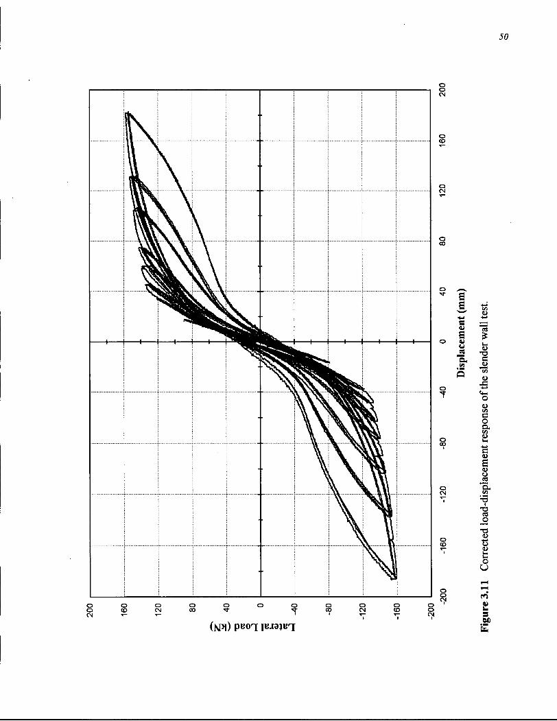
50

57
Beyond the initial uncracked range, the slope of the curve reduced (secondary slope). With
subsequent cycling of the specimen into larger displacements, the slope of the curve degraded
further. The process of degraded slope with increased deformations is often termed stiffness
degradation. Further cycling at the same displacement level showed little degradation in
stiffness from the first to the second cycle. No degradation was observed due to cycling from the
second cycle to the subsequent cycles.
Degradation of the secondary slope with moving from one displacement level to another agrees
in principle with the analytical results shown for the bending moment-curvature relationship
(Figure 2.7-a, Chapter 2).
Figure 3.12 shows, for clarity, the first cycle at each displacement level of the load-displacement
relation. The concept of upper-bound and lower-bound response discussed for the bending
moment-curvature relationship (Chapter 2) can also be used to represent the load-displacement
response under cyclic loading as well. The upper-bound load-displacement relation is the
response that may be obtained when loading the specimen monotonically to failure without
having been damaged from a previous load cycle (or alternatively, previously uncracked
response). The lower-bound load-displacement relation or severely cracked response is a
function of the previously attained displacement or drift level. Figure 3.12 highlights the upper
(monotonic) and lower-bound load-displacement responses. The upper-bound load-displacement
response was drawn as the envelope to the hysteresis loops. The lower-bound load-displacement
is the severely cracked response of the wall specimen when pushed to the maximum
displacement level (i.e., 200 mm displacement cycles).
The relation between the bending moment calculated at the critical joint versus the measured
rotation of the critical section is plotted in Figure 3.13. The moment-rotation relation provides
an indication of the flexural deformations exhibited plus any slippage of the longitudinal
reinforcement that may occur at the critical joint.
The bending moment at the critical section was calculated as the sum of the primary and
secondary moments. The primary moment was calculated as the product of the applied lateral
loading and the distance from the critical section location to the hydraulic actuator (37'-2.2",
11.333 m). The secondary moment was calculated as the sum of the vertical component of the

o
CM <U O O O O O O O O O O O 1 I-O CD CN 00 ^ 00 C\l CO O 3 CN - - , - ^ ' V Y W>

53
o
c > c > c >
o o m o o o
o o in
(uispf) iu3iuoi\T guipuag
"DTT
' in
0. >
•o 08 s o
m o £ °. o ° OS
O O
O O
O O If) o o o in
c > c > o C J
o o o
CM o o o
CO o o
o o
in o
I
c u s o
"a, CM u.
a> Q.
<u
C
c o
13
J3
e o a , <D u . C
o
p c ii S o e 60 C "3 c <u
X) •o m w 3 (S3 <U
i—(
s Ml
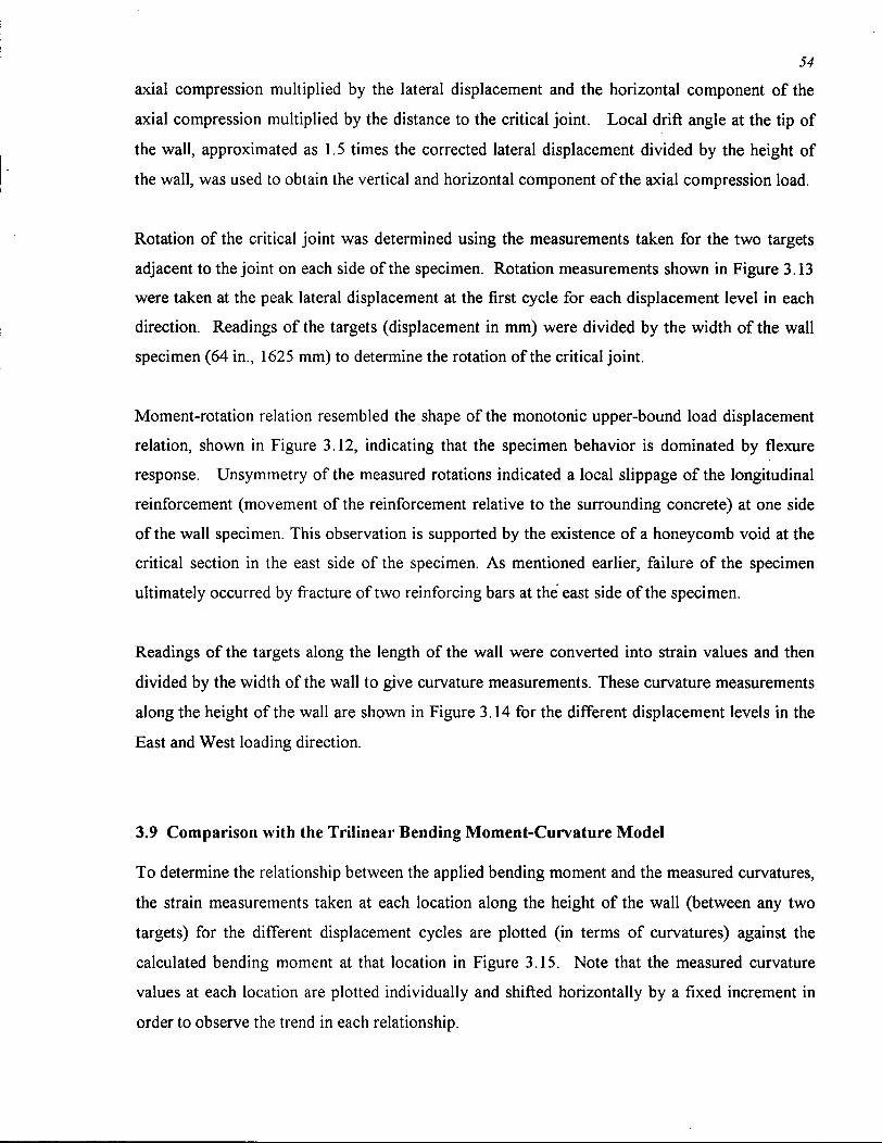
54 axial compression multiplied by the lateral displacement and the horizontal component of the
axial compression multiplied by the distance to the critical joint. Local drift angle at the tip of
the wall, approximated as 1.5 times the corrected lateral displacement divided by the height of
the wall, was used to obtain the vertical and horizontal component of the axial compression load.
Rotation of the critical joint was determined using the measurements taken for the two targets
adjacent to the joint on each side of the specimen. Rotation measurements shown in Figure 3.13
were taken at the peak lateral displacement at the first cycle for each displacement level in each
direction. Readings of the targets (displacement in mm) were divided by the width of the wall
specimen (64 in., 1625 mm) to determine the rotation of the critical joint.
Moment-rotation relation resembled the shape of the monotonic upper-bound load displacement
relation, shown in Figure 3.12, indicating that the specimen behavior is dominated by flexure
response. Unsymmetry of the measured rotations indicated a local slippage of the longitudinal
reinforcement (movement of the reinforcement relative to the surrounding concrete) at one side
of the wall specimen. This observation is supported by the existence of a honeycomb void at the
critical section in the east side of the specimen. As mentioned earlier, failure of the specimen
ultimately occurred by fracture of two reinforcing bars at the east side of the specimen.
Readings of the targets along the length of the wall were converted into strain values and then
divided by the width of the wall to give curvature measurements. These curvature measurements
along the height of the wall are shown in Figure 3.14 for the different displacement levels in the
East and West loading direction.
3.9 Comparison with the Trilinear Bending Moment-Curvature Model
To determine the relationship between the applied bending moment and the measured curvatures,
the strain measurements taken at each location along the height of the wall (between any two
targets) for the different displacement cycles are plotted (in terms of curvatures) against the
calculated bending moment at that location in Figure 3.15. Note that the measured curvature
values at each location are plotted individually and shifted horizontally by a fixed increment in
order to observe the trend in each relationship.

55
The data shown in Figure 3.15 is summarized in a different way in Figure 3.16 where the
measured curvatures at different locations over the height and at different displacement cycles
are plotted versus the bending moment calculated at that location. The measurements were taken
at the peak lateral displacements at the first cycle for each displacement level. No target
readings were taken for the lower-bound bending moment curvature relationship (i.e., severely
cracked response at 200 mm cycle). The predicted upper-bound bending moment-curvature
relationships (both nonlinear and trilinear) are also shown in the figure. These were determined
using the procedures described in Chapter 2. Comparison between the predicted and observed
relationships show good agreement. It is interesting to note that the more complex nonlinear
relationship compares no better to the experimental relationship than the simplified trilinear
relationship.
It should be mentioned that the increase in strength due to strain hardening of the reinforcement
as observed in the test is not captured in the proposed model. However, this increase in bending
moment at high curvatures compensates for the assumption that the lower-bound includes the
effect of some tension-stiffening beyond yielding of the reinforcement. See Section 2.6.4 (Case
E in Fig. 2.7-a).
3.10 Concluding Remarks
The experimental study conducted on a large-scale slender wall validated the bending moment-
curvature model. The experimentally calibrated bending moment - curvature model will now be
used to develop a general method to determine the linear flexural stiffness of concrete walls.
Up to this point in the thesis, only the measured curvatures and the calculated bending moments
were used in the comparison with the proposed analytical model. Where applicable in the
following chapters, additional test results will be used to validate predictions from the proposed
model.

e e
6000
5000 H
. 2 f «2 4000
PP
O) 3000
e •< 2000 u CS
Q 1000
*i JK ";+> "'A.'.''ie»..
East
5 6 7 8
6000
£ 5000
e . 2 ? 'S 4000 P3
<U 3000
e o u u e cs
Q
2000
1000
West
# * + "?""x, '""'A..
K '
—-o--- -12 mm ----- - 18 mm -—4— •24 mm - - * -•48 mm
+ -60 mm -75 mm
- - K • ••90 mm - - * -120 mm
— •150 mm -200 mm
10 11
<f> (rad/km)
—-o-- -12 mm —-•- 18 mm
•24 mm • * • • •48 mm
....+.. •60 mm --o— -75 mm • - K -•90 mm
• * • •120 mm ------ -150 mm
. . . . •200 mm
<f> (rad/km)
Figure 3.14 Measured curvature distribution along the wall height during the different lateral displacement cycles.
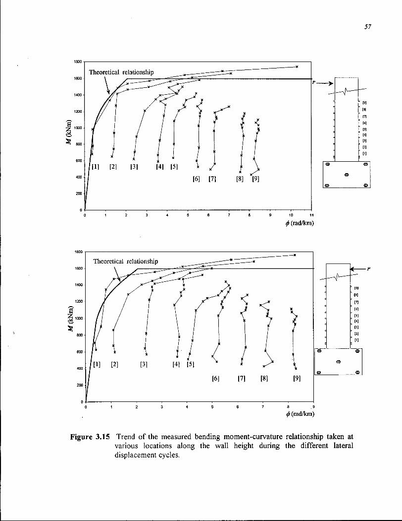
57
Figure 3.15 Trend of the measured bending moment-curvature relationship taken at various locations along the wall height during the different lateral displacement cycles.
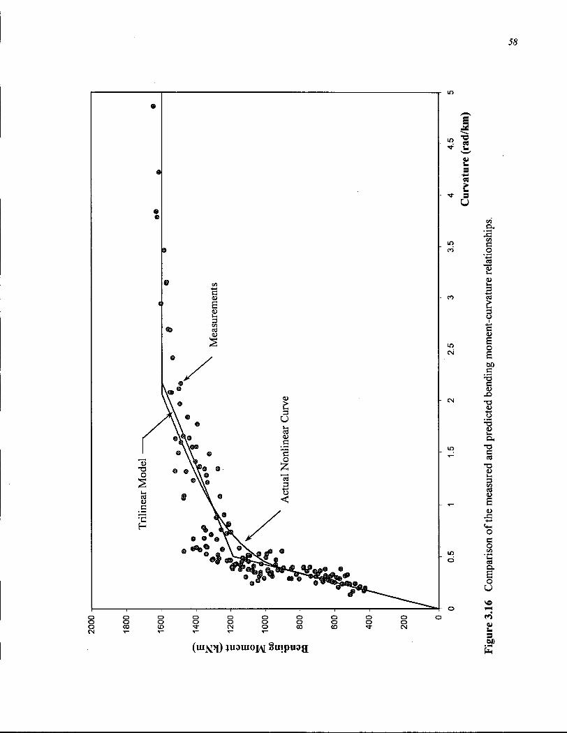

Chapter 4
Effective Flexural Stiffness of Concrete Walls
4.1 Introduction
The trilinear bending moment-curvature relationship (i.e., nonlinear stiffness model) developed
in Chapter 2, having been validated against the experimental results in Chapter 3, is used in this
chapter to determine a "linear" flexural stiffness that can be used for the linear seismic analysis
of concrete walls. The effective stiffness of a wall structure is determined by obtaining the linear
elastic-perfectly plastic (bilinear) equivalent of the actual nonlinear load-displacement
relationship. The effective stiffness is the slope of the linear elastic portion of the load-
displacement relation.
As seen from the slender wall test results, once concrete cracks, the flexural stiffness of the wall
reduces. Additional cracking due to cycling loading degrades the stiffness further and results in
a substantial reduction in the flexural stiffness. Degradation of stiffness due to cracking during
the cyclic motion of an earthquake is well recognized in the literature and known to increase the
fundamental period of a building, see Figure 4.1.
To account for the degradation of stiffness and similar to the proposed bending moment-
curvature model, the effective stiffness of the wall structure is expected to range from an upper-
bound effective stiffness (which corresponds to a wall that is loaded monotonically without
being previously cracked) to a lower-bound effective stiffness (which corresponds to a wall that
is severely cracked from the previous load cycles).
In the following, the use of the trilinear bending moment-curvature relationship in predicting the
actual nonlinear load-displacement relation of a wall structure is described. Characteristics of
the load-displacement relation are discussed and the effective linear stiffness (both upper-bound
and lower-bound) are determined. The influence of several important parameters on the
predicted flexural stiffness is examined and a general as well as a simplified procedure to
59

60
Figure 4.1 Typical lengthening of the fundamental period of a concrete wall due to the reduction in stiffness resulting from cracking during earthquake motion.
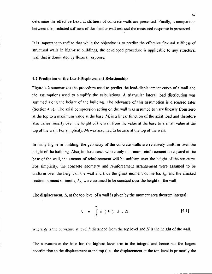
61
determine the effective flexural stiffness of concrete walls are presented. Finally, a comparison
between the predicted stiffness of the slender wall test and the measured response is presented.
It is important to realize that while the objective is to predict the effective flexural stiffness of
structural walls in high-rise buildings, the developed procedure is applicable to any structural
wall that is dominated by flexural response.
4.2 Prediction of the Load-Displacement Relationship
Figure 4.2 summarizes the procedure used to predict the load-displacement curve of a wall and
the assumptions used to simplify the calculations. A triangular lateral load distribution was
assumed along the height of the building. The relevance of this assumption is discussed later
(Section 4.3). The axial compression acting on the wall was assumed to vary linearly from zero
at the top to a maximum value at the base. Mi is a linear function of the axial load and therefore
also varies linearly over the height of the wall from the value at the base to a small value at the
top of the wall. For simplicity, Mi was assumed to be zero at the top of the wall.
In many high-rise building, the geometry of the concrete walls are relatively uniform over the
height of the building. Also, in those cases where only minimum reinforcement is required at the
base of the wall, the amount of reinforcement will be uniform over the height of the structure.
For simplicity, the concrete geometry and reinforcement arrangement were assumed to be
uniform over the height of the wall and thus the gross moment of inertia, Ig, and the cracked
section moment of inertia, Icr, were assumed to be constant over the height of the wall.
The displacement, A, at the top level of a wall is given by the moment area theorem integral:
where <fa is the curvature at level h distanced from the top level and H is the height of the wall.
H A [4.1]
o
The curvature at the base has the highest lever arm in the integral and hence has the largest
contribution to the displacement at the top (i.e., the displacement at the top level is primarily the

62

63
results of the curvatures near the base of the wall). Small error in the displacement results from
using the characteristics of the cross section at the base when the wall characteristics vary over
the height. Therefore, the load-displacement curve of a wall structure can be characterized by
the two non-dimensional parameters that describe the bending moment-curvature relationship of
the cross section at the base of the wall: the ratio of the cracked section moment of inertia to the
uncracked section (gross) moment of inertia, Icrl Ig, and the ratio of the linear bending moment to
the capacity of the wall section at the base, Mi I M„.
Prediction of a nonlinear load-displacement curve requires the application of Equation [4.1] to
determine the top displacement, A, at different load steps. The height of the wall was discretized
into several levels. Each level has its specific trilinear bending moment-curvature relationship
according to the assumed axial load at that level (Figure 4.2-f). At each load step, the bending
moment distribution along the height was computed, and the curvature at each level was
determined from the corresponding trilinear bending moment-curvature relationship. Integration
of the resulting curvature distribution gives the top displacement at this load step. The procedure
was repeated for several load steps and the complete load-displacement curve was determined.
Note that even though the bending-moment curvature relationship is piecewise linear, the load-
displacement relationship is nonlinear. Nonlinear curvature distribution along the height,
resulting form the cubic distribution of the bending moment, is the main reason.
The above procedure was implemented in program Wall-Tools and the program was used to
generate the load-displacement relationships shown in the following sections.
4.3 Characteristics of the Load-Displacement Relationships
The procedure just described was used to determine the load-displacement relationships of the
walls shown in Figure 4.3. Two different cross sections at the base of the wall were considered in
the example. The actual nonlinear load-displacement relations shown in the figure are for the
monotonic upper-bound response. A somewhat secondary slope follows the initial linear
uncracked gross section response of the load-displacement relation until the wall reaches its yield
strength/displacement. Bilinear approximation of the actual nonlinear load-displacement

64
relationship is needed to estimate the effective stiffness of the response. The effective stiffness of
the wall response is determined as the slope of the linear elastic portion of the bilinear
idealization.
FEMA 273 (1997) suggests the use of the secant to 60% of the yield strength as the elastic slope
of the bilinear idealization of the actual load-displacement curve when determining the
fundamental period of a structure. Paulay and Priestley (1992) suggest the use of an effective
secant stiffness to the nonlinear load-displacement curve that is based on 75% of the yield
strength or nominal strength of the concrete member. French and Schultz (1991) used the secant
to the load-displacement curve at 2/3 of the maximum load to idealize the actual nonlinear curve
with a bilinear approximation when examining the displacement history of several beam tests.
The secant to the nonlinear load-displacement curve at first yield of the reinforcement was used
by Priestley and Hart (1989) to define the effective stiffness for period and ductility calculations
of rectangular masonry walls.
For walls with a small amount of vertical reinforcement as shown in Figure 4.3 (common in
high-rise wall buildings constructed in British Columbia), the uncracked section response of the
load-displacement relationship is very significant. In addition, the secondary slope of the load-
displacement curve is nearly flat. Considering the effective stiffness as the secant at 3/4 of the
nominal/yield strength or alternatively at 2/3 or 3/5 of the maximum load results in a stiffness
value that is very close to the initial uncracked response and underestimates the effective yield
displacement of the wall response (see Figure 4.3).
While the equivalent bilinear idealization of the load-displacement relationship using the secant
to the first yield of reinforcement may provide a more appropriate estimate of the yield
displacement (Priestley and Hart, 1989), it certainly gives a lower estimate of the effective
stiffness needed for the calculation of the elastic fundamental period of the wall structure. Also,
it has been shown (Section 2.2) that relating the stiffness to the yield curvature does not seem to
capture the elastic deformations of such walls. Note that the low values of effective stiffness
recommended in the commentary to the New Zealand concrete code (Figure 1.1) are based on
the recommendation of Priestley and Hart (1989). The SEAOC Blue Book (1996) indicates that
this stiffness recommendation "can yield unrealistically low values of stiffness".

s o b
Shape "A" Shape "B" 6.0 m
p,= 1.0% d
p. = 0.25% 6.0 m
T2 l l
0.25
0.4
Jl 0.25%
p ( = 0.5%
P = 0.1 fc'Ag f' = 50 MPa fy = 400 MPa
1600
1400
1200
1000
800
600
400
200
2400
2000
< ? 1600 g
1200
800
400
10 20
10
Equivalent bilinear idealization
/ / Actual nonlinear curve
Shape A
n 0.75 V„
// A 0.67 Vb
• 0.60 Vb
30 40 50 60 70 80 90 100
A (mm)
/ / Shape B
// m 0.75 Vb
0.67 Vb
0.60 Vb
15 20 25 30 35 40 45 50 A (mm)
Figure 4.3 Load-displacement characteristics for typical wall sections.

66
Since a good representation of the nonlinear load-displacement curve should also involve a good
representation of the actual energy absorbed by the real inelastic load-displacement curve (i.e.,
area under the curve) in addition to the provision of a realistic estimate of the effective yield
displacement, it is suggested that the equivalent bilinear idealization of the actual nonlinear load-
displacement curve is the one that has the same area under both curves (i.e., equal energy).
FEMA 273 (1997) also stated that the use of the specified secant stiffness at 60% of the yield
strength to determine the bilinear equivalent of the actual nonlinear load-displacement
relationship is an approximate measure with the recommendation to evaluate the use of this
criteria, "the best choice may be to have approximately equal area under both curves". This
criterion of equal area under the actual nonlinear and the idealized bilinear load-displacement
curves (equal energy under both curves) was used to determine the bilinear equivalent of the
load-displacement curve. Further discussion and comparison of the different assumptions to
determine the bilinear equivalent of the load-displacement curve are provided in Section 4.4.
Figure 4.4 shows the load-displacement curve of the wall example shown in Figure 4.3 (Shape
A). Two different load distributions were used: the triangular load distribution (as shown
previously in Figure 4.3 and repeated here for comparison) and the first mode lateral forces.
The results of the analyses are shown in terms of the top displacement of the wall as well as the
displacement at the center of lateral load. In each case, the equivalent bilinear idealization with
the same area under the actual load-displacement curve is also shown. Note that the plots are
presented with non-dimensional axes where the load is divided by the maximum load and the
displacement is divided by the corresponding yield displacement.
The results of the analyses indicate that the stiffness of the elastic portion of the bilinear response
of the wall or the "effective stiffness" as a ratio of the initial (uncracked) stiffness is reasonably
independent of the assumed load distribution and the location of measured displacement. This
stiffness value of 0.75-0.78 Ig is unique to the cross section characteristics of the specific wall.
4.4 Determination of Effective Flexural Stiffness of Concrete Walls
Both the upper-bound and lower-bound effective stiffnesses of a wall structure were determined
by obtaining the bilinear equivalent of the actual load-displacement relationship. The load-

67

68
displacement relationship of a wall, characterized by the two non-dimensional parameters that
describe the cross section at the base of the wall: Icr/ Ig, and Mi I M„, was determined using the
procedure described in Figure 4.2. The equivalent bilinear idealization of the load-displacement
curve was determined with the same area under both curves and the effective stiffness was
determined as the elastic stiffness of the idealized relation.
The effective flexural stiffness was determined for a variety of possible values of the two non-
dimensional parameters that characterize the load-displacement relationship of a wall structure
and the resulting effective stiffnesses (represented as a fraction of the gross moment of inertia, Ie
IIg) are plotted in Figure 4.5.
Figure 4.5 shows the variation of the effective stiffness with any possible variation in the
characteristics of the section at the base of the wall. As shown, the effective stiffness can be
anywhere between 0.0 and 1.0 and is influenced by the ratio Icrl Ig and/or the ratio Mi IM„.
The effective stiffness results shown in Figure 4.5 can be approximated by the following
expression:
e _ cr I ~ I g g
M
\ n J -2
M,
\ n J
' I \-JBL [4.2]
Where the exponent a, and b are defined in Table 4.1. Figure 4.6 compares results from the
simple expression, Equation [4.2], with the curves of Figure 4.5. Very good agreement is found.
Before using the above procedure to determine the effective flexural stiffness for various wall
structures and examine the influence of the important parameters that affect the stiffness, it is
useful to use the fundamental approach illustrated in Figure 4.5 to confirm the premises of equal
area criteria to approximate the nonlinear load-displacement relation with a bilinear curve.
Figure 4.7 compares the effective stiffness values determined using the equal area criteria to
those computed using a secant stiffness to a point on the actual load-displacement curve located
at: 75%, 67% and 60% of the yield strength. As mentioned earlier, these have been used by
others to determine the equivalent elastic stiffness. The different procedures yield very similar
results for small values of Mi I M„. On the other hand, very different results are obtained for

69
7/7

Table 4.1 Values of the exponent a and b for Equation [4.2].
Ic/I8 a b
0.05 3.8 6.0 0.10 2.8 4.4 0.15 2.3 3.6 0.20 2.0 3.1 0.25 1.9 3.0 0.30 1.8 2.9 0.35 1.7 2.8 0.40 1.6 2.6 0.45 1.5 2.4 0.50 1.4 2.2 0.55 1.3 2.0 0.60 1.2 1.8


72
>
+->
a -*-» o to -o o
1 CD
Uc
(50
c ii a
T 3 t« 01
u ,
3 ii
53 m
1) CO
5 3 »
eu 53
o \3 — CO
o .2 00 0)
'S 53
s .s O
U ^ U l a
s
7 / 7

73
large values of Mi I M„ (when the initial gross stiffness exceeds the prescribed portion of the
yield strength on the load-displacement relation). Large values of the ratio Mi I M„ occur for
example when there is a minimum amount of vertical reinforcement in the wall as shown
previously in Figure 4.3. The equal area method provides more conservative, and it is believed
more appropriate, values of the effective stiffness.
4.5 Trend of Stiffness Variation
Figure 4.5 provides a fundamental method to determine the effective stiffness of a wall structure
knowing the four parameters that characterize the cross section at the base: Ig, Icr, Mi, and M„.
Increasing the ratio Icrl Ig and/or the ratio Mi I M„ increases the effective stiffness. A change in
geometry or material property of the section at the base that affects any of the four parameters
will have an influence on the predicted stiffness of the wall.
It is useful then to examine the influence of some important variables (that affect the four
parameters) on the stiffness values of some typical concrete walls. The main variables are: the
axial compression acting on the wall; the concrete geometry; the amount and distribution of
vertical reinforcement; the concrete compressive strength; and the yield strength of the vertical
reinforcement.
In the following, the influence of each of the main variables is examined and the significance of
each variable on the variation of stiffness is illustrated. Results are shown for the upper-bound
and lower-bound effective stiffness.
4.5.1 Axial Compression Acting on the Wall
Effect of the axial compression acting on the wall is widely recognized (e.g., Priestley and Hart
1989, Council, 1992) as an important parameter affecting wall stiffness. Figure 4.8-a shows the
variation of the effective stiffness with the axial compression acting on a rectangular wall cross
section. Increasing the axial compression results in an increase in bothM; andM„.
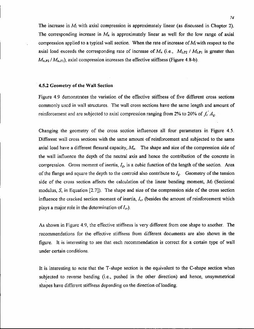
74
The increase in Mi with axial compression is approximately linear (as discussed in Chapter 2).
The corresponding increase in M„ is approximately linear as well for the low range of axial
compression applied to a typical wall section. When the rate of increase of Mi with respect to the
axial load exceeds the corresponding rate of increase of M„ (i.e., MI,YI I M , P I is greater than
M „ , P 2 /M„ ,PI ) , axial compression increases the effective stiffness (Figure 4.8-b).
4.5.2 Geometry of the Wall Section
Figure 4.9 demonstrates the variation of the effective stiffness of five different cross sections
commonly used in wall structures. The wall cross sections have the same length and amount of
reinforcement and are subjected to axial compression ranging from 2% to 20% of fc Ag.
Changing the geometry of the cross section influences all four parameters in Figure 4.5.
Different wall cross sections with the same amount of reinforcement and subjected to the same
axial load have a different flexural capacity, M„. The shape and size of the compression side of
the wall influence the depth of the neutral axis and hence the contribution of the concrete in
compression. Gross moment of inertia, Ig, is a cubic function of the length of the section. Area
of the flange and square the depth to the centroid also contribute to Ig. Geometry of the tension
side of the cross section affects the calculation of the linear bending moment, Mi (Sectional
modulus, S, in Equation [2.7]). The shape and size of the compression side of the cross section
influence the cracked section moment of inertia, Icr (besides the amount of reinforcement which
plays a major role in the determination of Icr).
As shown in Figure 4.9, the effective stiffness is very different from one shape to another. The
recommendations for the effective stiffness from different documents are also shown in the
figure. It is interesting to see that each recommendation is correct for a certain type of wall
under certain conditions.
It is interesting to note that the T-shape section is the equivalent to the C-shape section when
subjected to reverse bending (i.e., pushed in the other direction) and hence, unsymmetrical
shapes have different stiffness depending on the direction of loading.
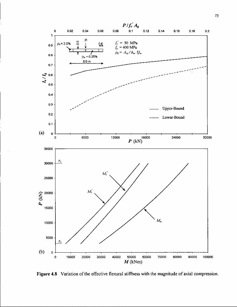
75
0.02 0.04 0.06 P/fcA8
0.08 0.1 0.12 0.14 0.16 0.18 0.2 1
0.9
0.8 H
0.7
0.6 ^
0.5
0.4 H
0.3
0.2
0.1
(a) o
35000
30000
u> P p 2=2.0% d
25000
20000
15000
10000
5000
' I 1 t " pw = 0.25% 6.0 m
fe = 50 MPa fy = 400 MPa pz = A„ I by,. %lw
Upper-Bound
Lower-Bound
-+-6000 12000 18000 24000
P (kN) 30000
(b) o4 0 10000 20000 30000 40000 50000 60000 70000 80000 90000 100000
M (kNm)
Figure 4.8 Variation of the effective flexural stiffness with the magnitude of axial compression.
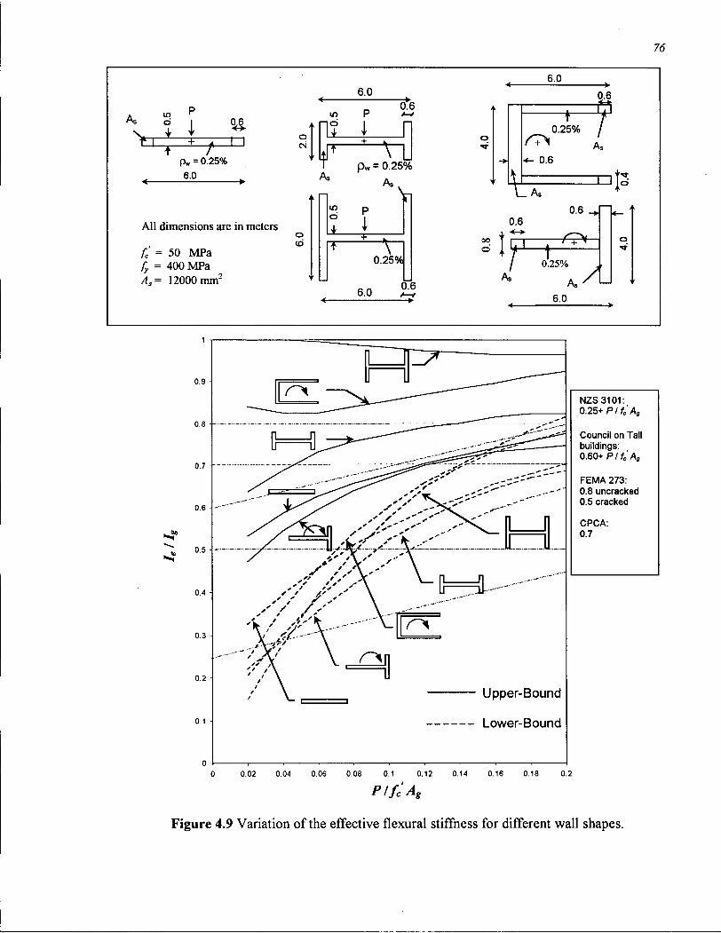
76
6.0 6.0
0.6 in d
Pw = 0.25% 6.0
It
All dimensions are in meters
A, p w = 0.25%
A,
fc = 50 MPa fy = 400 MPa /!.= 12000 mm2
o CD
V p
I 0.25W
0.6
«- 0.6
t J 0.25% /
= 13 0.6
/ 0.25%
0.6
6.0 0.6 As 6.0
0.1
U p p e r - B o u n d
L o w e r - B o u n d
NZS3101: 0.25+ P / f e X
Council on Tall buildings: 0.60+ PlfcAg
FEMA 273: 0.8 uncracked 0.5 cracked
CPCA: 0.7
0 0.02 0.04 0.06 0.08 0.1 0.12 0.14 0.16 0.18 0.2
Ptfc'Ag
Figure 4.9 Variation of the effective flexural stiffness for different wall shapes.

77
4.5.3 Amount and Distribution of the Vertical Reinforcement
Figure 4.10 shows the variation of the effective stiffness for different amounts of vertical
reinforcement concentrated in the boundary zone of a rectangular wall section. Increasing the
amount of reinforcement increases the flexural capacity of the wall section, M„, as well as the
cracked section moment of inertia, Icr. The increase inM„ reduces the effective stiffness whereas
the increase in Icr increases the stiffness value. Whichever of these two dominates the response
will control whether there is an increase or decrease in the resulting effective stiffness.
For the rectangular wall shape, the upper-bound effective stiffness is reduced with the increase of
the amount of vertical reinforcement whereas the lower-bound effective stiffness is increased
with increasing the amount of the reinforcement (Fig. 4.10-a).
Note that the increase in the value of M„ and Icr (when increasing the amount of reinforcement)
is the same for both the upper and lower stiffness prediction, however, it is the range of the Mi I
M„ ratio that makes the difference. Upper-bound stiffness prediction involves higher values of Mi
I M„ ratios in which a small change of M„ and consequently Mi I M„ makes a drastic change in
the stiffness value (see Figure 4.5). In other words, for high values of Mi I M„ (upper-bound
stiffness prediction, Mi I M„), the increase in M„ and the consequent reduction of Mi I M„ ratio
dictate the predicted stiffness, whereas for the lower-bound effective stiffness prediction (lower
range of Mi I M„ values) the effect of increase in Icr value with the increased amount of
reinforcement controls the resulting stiffness value.
A reduction in the value of the upper-bound effective stiffness with an increasing amount of
reinforcement should not be confused with the basic definition of stiffness where a stiffer
structure is displaced less when subjected to the same force (or alternatively, stiffer response of
the structure requires higher force to displace the same amount of deflection). The force-
displacement characteristics of two cases of different amounts of reinforcement, for both the
upper and lower-bound predictions, are shown in Figure 4.11. As the amount of reinforcement
increases, the secondary slope of the curve becomes larger (which is a function of Icr) and the
amount of displacement is less for the same lateral force (i.e., stiffer response). However, the
slope of the bilinear approximation that gives an equivalent area to the actual load-displacement
curve is smaller when the amount of reinforcement is increased for the upper-bound predictions.
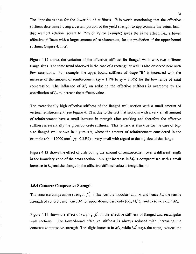
78
The opposite is true for the lower-bound stiffness. It is worth mentioning that the effective
stiffness determined using a certain portion of the yield strength to approximate the actual load-
displacement relation (secant to 75% of V\> for example) gives the same effect, i.e., a lower
effective stiffness with a larger amount of reinforcement, for the prediction of the upper-bound
stiffness (Figure 4.11-a).
Figure 4.12 shows the variation of the effective stiffness for flanged walls with two different
flange sizes. The same trend observed in the case of a rectangular wall is also observed here with
few exceptions. For example, the upper-bound stiffness of shape "B" is increased with the
increase of the amount of reinforcement (fif- 1.5% to py= 3.0%) for the low range of axial
compression. The influence of M„ on reducing the effective stiffness is overcome by the
contribution of Icr to increase the stiffness value.
The exceptionally high effective stiffness of the flanged wall section with a small amount of
vertical reinforcement (see Figure 4.12) is due to the fact that sections with a very small amount
of reinforcement have a small increase in strength after cracking and therefore the effective
stiffness is essentially the gross concrete stiffness. This remark is also true for the case of big-
size flanged wall shown in Figure 4.9, where the amount of reinforcement considered in the
example (As = 12000 mm2, /3f=0.35%) is very small with regard to the big size of the flange.
Figure 4.13 shows the effect of distributing the amount of reinforcement over a different length
in the boundary zone of the cross section. A slight increase in M„ is compromised with a small
increase in Icr, and the change in the effective stiffness value is insignificant.
4.5.4 Concrete Compressive Strength
The concrete compressive strength, fc, influences the modular ratio, n, and hence Icr, the tensile
strength of concrete and hence Mi for upper-bound case only (i.e., Mi ), and to some extent M„.
Figure 4.14 shows the effect of varying fc on the effective stiffness of flanged and rectangular
wall sections. The lower-bound effective stiffness is always reduced with increasing the
concrete compressive strength. The slight increase in M„, while Mi stays the same, reduces the

T3 "D C C 3 3 O O m m i i i cu a> CL > 3-J
o ^
cO
GO I -CO
I u I i c3
i s o <2 c "S eO o
'•E > o CO
3 o
e to
u 1-1
I T 3
CO CO
re!
ID 53 <u
_> V* o
X! -*-» o c o '13 •c CO
>
u s
• mm
fa

80
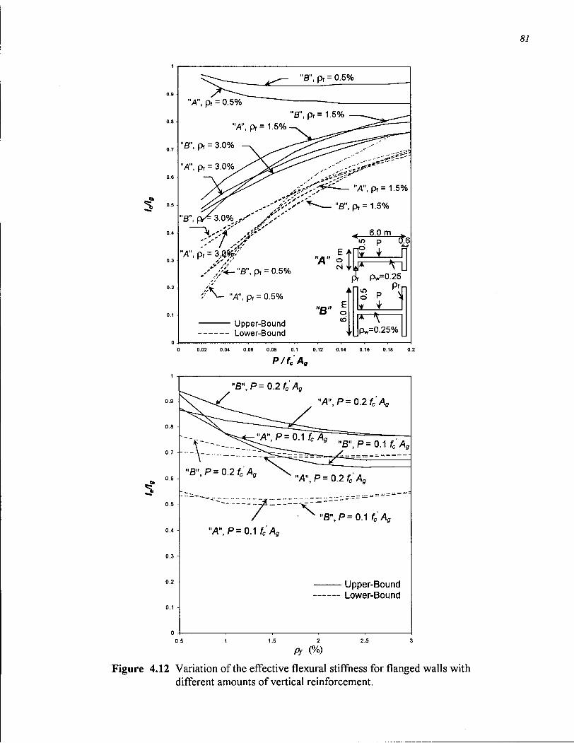
1
0 -I , , , , , , , , , 1 0 0.02 0.04 0 06 0.08 0.1 0.12 0.14 0.16 0.18 0.2
P/fe'Ag
"B",P=0.2fc Ag
"A",P= 0.2fcAg
t It All p — ~Q^V^====sssa=" :— 9 «B",P=0AfcAg
- v -"B", P= 0.2 fc Ag \
"A",P= 0.2 fc Ag
' • - / - - • • x " B \ P = 0.1 fcAg
"A",P= 0.1 fcAg
Upper-Bound Lower-Bound
0.5 1 1.5 2 2.5 3
Pf (%)
Figure 4.12 Variation of the effective flexural stiffness for flanged walls with different amounts of vertical reinforcement.
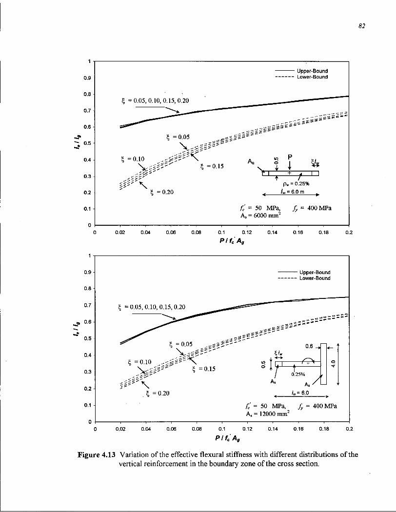
82
Upper-Bound Lower-Bound
% =0.05,0.10,0.15,0.20
it =0.05 V
% =0.10
S S S S
% =0.20
§ =0.15 As
lO O
A.
P
"T"
p„ = 0.25% L = 6.0 m
fc = 50 MPa, fy = 400 MPa A, = 6000 mm2
0.02 0.04 0.06 0.08 0.1 0.12 0.14 0.16 0.18 PlfC Ag
0.2
Upper-Bound Lower-Bound
0.7
0.6 -
0.5 -
% =0.05,0.10,0.15,0.20
% =0.05 .-s
% =0.10 , - ^ ^ * \ V - ^ ' " 1=0.15
I = 0.20
- J5 0.6 .
0 . 2 5 %
A, /„=6.0
4 A fc = 50 MPa, fy = 400 MPa A s = 12000 mm2
0.02 0.04 0.06 0.08 0.1
Plfc'Ag 0.12 0.14 0.16 0.18 0.2
Figure 4.13 Variation of the effective flexural stiffness with different distributions of the vertical reinforcement in the boundary zone of the cross section.

83
ratio of Mi I M„. The modular ratio, «, is also reduced (due to higher value of Ec) and hence Icr.
The upper-bound effective stiffness is influenced by bothM; andM„. Increasing fc will increase
Mi (due to higher concrete cracking strength) and M„ (due to stronger concrete in compression)
while reducing Icr.
Higher Mi value results in higher effective stiffness whereas higher M„ and/or lower Icr result in
lower effective stiffness. When the effect of the increased Mi exceeds the combined effect of
higher M„ and lower Icr, the result is higher upper-bound effective stiffness with increasing fc as
seen for the flanged wall shown in Figure 4.14-a. The reverse effect is seen for rectangular
walls shown in Figure 4.14-b where the upper-bound effective stiffness is mostly reduced with
increasing fc .
4.5.5 Yield Strength of the Vertical Reinforcement
The yield strength of the vertical reinforcement influences only the capacity of the wall cross
section, M„. Increasing the yield strength of the reinforcement results in higher M„ and hence a
lower ratio of Mi I M„. The resulting effective stiffness is therefore reduced with an increase in
the yield strength. Figure 4.15 demonstrates the effect of changing the yield strength of the
vertical reinforcement on the effective stiffness of both rectangular and flanged wall sections.
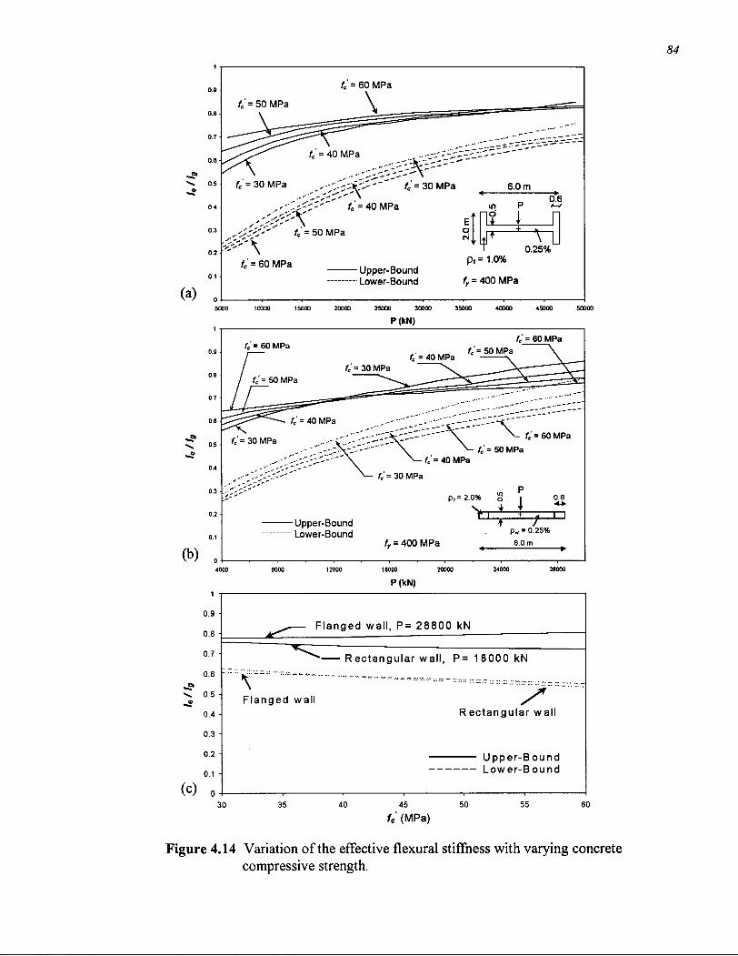
(a)
- Upper-Bound - Lower-Bound
p,= 1.0% 0.25%
5000 10000 15O0O 20000 25000 30000 35000 40000 45000 50000
P(kN)
-S1
(b)
U = 60 MPa
fe = 30 MPa 60 MPa fe = 50 MPa
U = 40 MPa U = 30 MPa
-Upper-Bound Lower-Bound
pz=2.0K> £ |
Z£2 p„ = 0.25% 6.0 m
16000
P(kN)
0.9 •
0.8 -
0.7 -
0.6 -
0.5 -
0.4 -
0.3 -
0.2
0.1 -
(c) 0 --
F l a n g e d wa l l , P= 2 8 8 0 0 kN
F l a n g e d wa l l
R e c t a n g u l a r w a l l , P= 1 8 0 0 0 kN
Rectangular w a l l
U p p e r - B o u n d L o w e r - B o u n d
30 35 40 45 fe (MPa)
50 55 60
Figure 4.14 Variation of the effective flexural stiffness with varying concrete compressive strength.
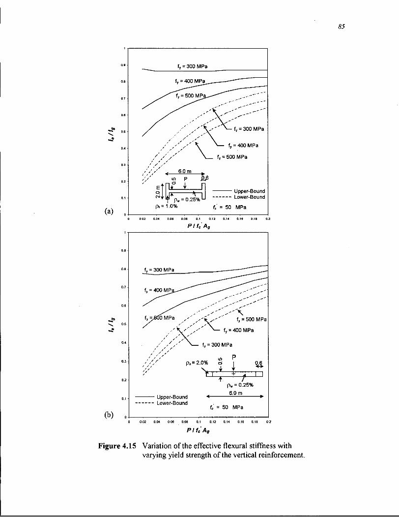
85
fy = 300 MPa
0 0.02 0.04 0.06 0.08 0.1 0.12 0.14 0.16 0.16 0.2
Plfe'Ag 11
09
(b) 0J , . . . . . . . . 1 0 0.02 0.04 0 06 0.08 0.1 0.12 0.14 0.16 0.18 0.2
Plfe'Ag
Figure 4.15 Variation of the effective flexural stiffness with varying yield strength of the vertical reinforcement.
86
4.6 Recommendations for Effective Flexural Stiffness of Concrete Walls
Results shown in the previous section indicate that the effective flexural stiffness of concrete
walls can vary greatly (from as little as 0.1 Ig to as high as 1.0 Ig ) depending on several
parameters: magnitude of axial compression, geometry of the cross section, amount of vertical
longitudinal reinforcement, yield strength of the reinforcement and the concrete compressive
strength. The very large variation in effective stiffness that is recommended by the various
documents (see Section 1.3) does actually exist in different wall types. The challenge is to
identify which walls have what effective stiffness. .
In this section, two methods to predict the effective flexural stiffness are presented: a general
method and a simplified method. The general method captures the influence of all the various
parameters that affect the stiffness value and provides an accurate estimate of the effective
flexural stiffness. To determine the effective stiffness using the general method, the
reinforcement and material properties of the cross section at the base of the wall are needed. As
the amount of reinforcement is not normally known at the start of the analysis, designers need a
quick estimate of the effective flexural stiffness to initiate the design process. The simplified
method is intended to provide an estimate of the effective flexural stiffness of a wall structure.
4.6.1 General Method for Determining Effective Flexural Stiffness
An accurate estimate of the effective flexural stiffness of concrete wall building (both the upper-
bound and lower-bound) can be determined using the following procedure considering the cross
section near the base of the wall building:
• Determine the ratio of cracked section moment of inertia Icr, and the uncracked (gross)
section moment of inertia Ig. The value of Icr for typical wall sections can be determined
using Figure 2.9. For other wall shapes, use program Wall-Tools.
• Determine the ratio of linear bending moment Mi and the flexural capacity M„ of the
cross section near the base of the wall. Mi can be determined using Equation [2.7]. To
determine the upper-bound response and consequently the upper-bound stiffness of the
wall, use B= 1.5 in Equation [2.7], while to determine the lower-bound stiffness use B =
0.
• Determine the effective stiffness of the wall Ie I Ig from Figure 4.5 or from Equation [4.2].
87
Figure 4.5 along with Equation [4.2] and Table 4.1 are reproduced together in Figure 4.16 for
convenience. It is worth mentioning that Figure 4.16, besides providing an accurate estimate of
the stiffness considering the effect of all important parameters, is a fundamental procedure and is
not based on the assumptions involved in the development of the specific trilinear bending
moment-curvature relationship presented in Chapter 2. Any theoretical bending moment-
curvature relationship can be approximated using any convenient trilinear idealization (i.e., a
bilinear idealization of the elastic deformations), and the two ratios of the idealized response
(secondary slope to initial slope, and bending moment at the end of the first linear segment to the
plastic moment capacity) can be used to determine the effective stiffness based on the equal area
approach from Figure 4.16.
4.6.2 Simplified Method for Determining Effective Flexural Stiffness
As mentioned, a complete description of the cross section at the base of the wall must be known
in order to accurately determine the effective stiffness using the general method. This is in
general the case for the design checker (checking the completed design) or for a design peer
review which is a common practice among structural design jurisdictions throughout the world.
Reinforcement details of the wall cross sections are not known until the design is completed and
hence to establish the design process and carry out the structural analysis of the building, an
estimate of the effective flexural stiffness of the wall sections is needed. The intent of the
simplified procedure is to capture the influence of the several parameters, previously discussed in
Section 4.5, on the effective stiffness in an approximate way and provide a quick estimate of the
flexural stiffness that can be used to start the design process.
A simple approximate estimate of the ratio of effective stiffness to gross stiffness can be a single
number similar to what is currently recommended in many documents. However, based on the
results presented earlier, it is more appropriate to link the effective stiffness to the axial
compression acting on the wall since it is a major factor that affects the stiffness and has been
recognized and used by others (Priestley and Hart 1989, Council 1992).
To develop simple expressions for both the upper-bound and lower-bound effective stiffness
values of wall structures, several common practical configurations of the cross section at the base
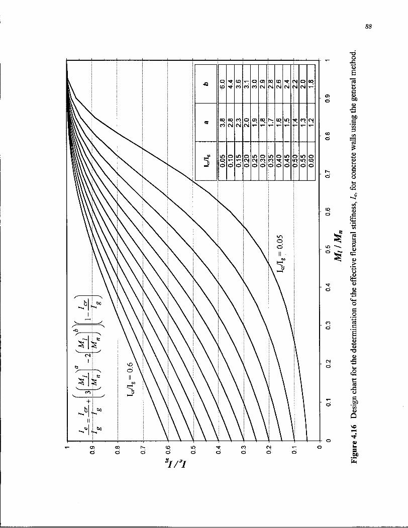
89
of the wall were examined and these are shown in Figures 4.17 through 4.22. In each
configuration (shape), the practical minimum and maximum amounts of vertical reinforcement in
the boundary zones or the flanges were considered. Concrete compressive strength that ranges
between 40 to 60 MPa (and the corresponding Ec and fcr) were varied in each shape. For each
geometry, upper and lower-bound effective flexural stiffness were determined for an applied
axial compression ranging from 2% to 20% of fc Ag. Variation in the yield strength of the
vertical reinforcement was not considered in this study since the majority of reinforced concrete
structures currently built in North America have 400 MPa or 414 MPa (Grade 60) yield strength
steel.
It is seen from the figures for the different geometries considered in this study that, despite the
scatter, the upper-bound effective stiffness can be reasonably approximated by the expression
suggested by Paulay (Council 1992):
1 - o .6 + - [4.3-a] g J c g
The lower-bound effective flexural stiffness shows less scatter particularly for rectangular and
flanged wall sections. A steep increase in the effective stiffness is found when increasing the
applied axial compression. The following simple expression is proposed for the lower-bound
effective stiffness:
I P - ^ = 0.2 + 2.5 [43-bl I f 'A 1 1
g J c g
Note that the upper-bound effective stiffness shall be less or equal to the gross section stiffness.
The lower-bound effective stiffness shall never be taken higher than the upper-bound effective
stiffness value. The two simple expressions (Eq. [4.3] a and b) are shown in Figures 4.17 to 4.22
for comparison.
While the proposed simplified expressions provide a reasonable approximation for most walls,
there are certain conditions (e.g., flanged walls with an amount of the vertical reinforcement in
the flange that is less than 1%) when the actual stiffness deviates considerably from the simple
expressions. For this reason, it is suggested that the general method be used whenever necessary
to estimate the effective stiffness of concrete walls. A more elaborate and extensive analyses for
different wall shapes with various geometrical dimensions are provided in Appendix E.

90
0.9
0.8
0.7
0.6
^» 0.5
0.4
0.3
0.2
0.1
As; in o
V 1 24 Cv = 0.25% 6.0 m
60 MPa
60 MPa
,4.0% ,'S,'Ss',*<
</ \
40 MPa, 3.0%
40 MPa, 2.0%
40 MPa, 1.0%
60 MPa, 2.0%
60 MPa, 1.0%
Upper-Bound Lower-Bound Simplified Method
0 0.02 0.04 0.06 0.08 0.1 0.12 0.14 0.16 0.18 0.2 P/fcAg
Figure 4.17 Comparison of the suggested simplified expressions for determining the effective flexural stiffness with a variety of results for rectangular walls.

91
0.9
0.8
0.7
0.6
0.5
0.4
0.3
0.2 -f
0.1
fc = 60 MPa, pf = 0.5%
40 MPa
40 MPa, 0.5%
v / 60 MPa, 4.0% y /'^
' ' / \ 60 MPa, 2.0%
60 MPa, 1.0%
60 MPa, 0.5%
V P
0.25%
6.0 m 0.6
Upper-Bound Lower-Bound Simplified Method
0 0.02 0.04 0.06 0.08 0.1 0.12 0.14 0.16 0.18 0.2
P/fc'Ag
Figure 4.18 Comparison of the suggested simplified expressions for determining the effective flexural stiffness with a variety of results for flanged walls.

92
0.9 H
0.8
0.7
0.6
0.5
0.4
0.3
0.2
0.1
B, fc = 40 MPa
yy\ 0.3
co o
A, fc = 60 MPa
A, fc = 40 MPa
/ 0.25%
0.3 .
pf /
i
+-
o
f
(b
6.0 m
Upper-Bound Lower-Bound Simplified Method
A: f>r = 0.5%, Asz= 1.0% B : pr = 3.0%, AS2 = 4.0%
0 0.02 0.04 0.06 0.08 0.1 0.12 0.14 0.16 0.18 0.2
P/fc'Ag
Figure 4.19 Comparison of the suggested simplified expressions for determining the effective flexural stiffness with a variety of "T" shaped walls (flange in tension).

Figure 4.20 Comparison of the suggested simplified expressions for determining the effective flexural stiffness with a variety of "T" shaped walls (flange in compression).

Figure 4.21 Comparison of the suggested simplified expressions for determining the effective flexural stiffness with a variety of "C" shaped walls (flange in tension).
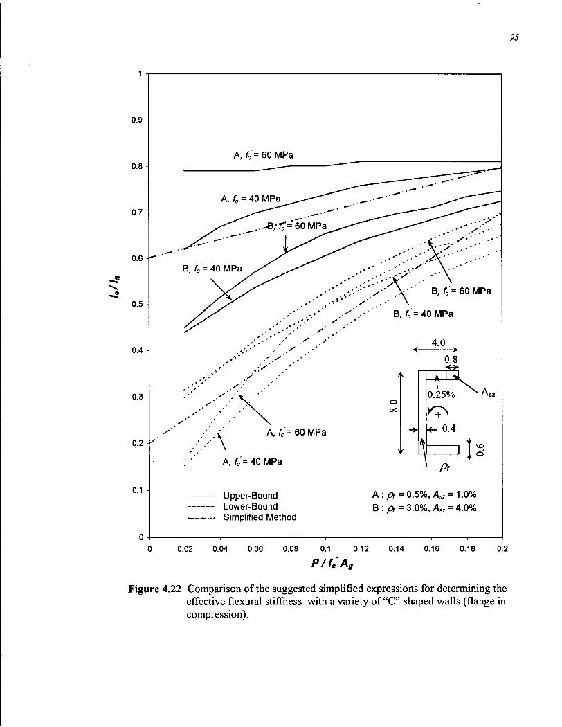
95
S1
0.9
0.8
0.7
0.6 - r
0.5
0.4
0.3
0.2
0.1
0 -I
A, fc = 60 MPa
A, fc = 40 MPa
Upper-Bound Lower-Bound Simplified Method
A : p, = 0.5%, Asz= 1.0% B:pf = 3.0%, Asz = 4.0%
0 0.02 0.04 0.06 0.08 0.1 0.12 0.14 0.16 0.18 0.2
P/fc'Ag
Figure 4.22 Comparison of the suggested simplified expressions for determining the effective flexural stiffness with a variety of "C" shaped walls (flange in compression).

96
4.7 Comparison of Predicted Stiffness with Slender Wall Test Results
The upper-bound load-displacement relation of the slender wall specimen, shown previously in
Chapter 3, Figure 3.12, is compared with the predicted bilinear load-displacement relation in
Figure 4.23. The effective elastic stiffness (I, = 0.79 Ig) was determined using the general
method.
The predicted lower-bound effective stiffness is compared with the ascending ramp of the
hysteresis loops for each of the last four displacement/drift levels in Figure 4.23-b. Again, the
general method was used to predict the elastic effective stiffness (7, = 0.39 Ig). Because of the
observed degradation in stiffness from the first cycle to the second cycle, the loading portion of
the second cycle, rather than the first cycle, at each displacement level is shown in the figure.
The lower-bound effective stiffness is related to the severely damaged and degraded response.
Each cycle is labeled with the maximum drift ratio attained during the first cycle. The global
drift ratio is the maximum displacement divided by the height of the wall.
The bilinear load-displacement relations shown in Figure 4.23 are estimated from the elastic
analysis of a cantilever wall of 11.333 m subjected to a single concentrated lateral load at the top.
The yield displacement, Ay, is estimated from the equation:
A v = F H 3 [4.4] y 3 E i 1 1
c e
where, H, is the height of the wall and, F, is the maximum lateral load computed as the capacity
of the flanged wall specimen over the height of the wall (i.e., M„ I FT). Ie distinguishes between
the upper and lower-bound bilinear load-displacement relations.
It is interesting to compare the measured load displacement relationship (for both the upper-
bound and lower-bound) with the bilinear load-displacement relation determined using the
recommended stiffness from the Commentary to the Canadian concrete code (CPCA 1995) in
Figure 4.24, and the Commentary to the New Zealand Standard (NZS 3101 1995) in Figure 4.25.
The two codes use a very similar philosophy for the seismic design of concrete walls and yet
these documents differ by a factor of two regarding the effective stiffness.

97
It is clear that the 70% of Ig suggested in the CPCA Handbook (Fig. 4.24) compares well to the
upper-bound response (or previously uncracked response) of the wall specimen but not very well
to the lower-bound response. The recommendation of the commentary to the NZS, on the other
hand, gives a conservative estimate of even the lower-bound stiffness at high drift levels.
4.8 Concluding Remarks
It is suggested that when estimating the maximum expected drift of a building, designers should
estimate the period and the corresponding forces and displacements using the lower-bound
effective stiffness for a severely cracked response of the wall. The upper-bound effective
stiffness may be used when estimating the seismic design actions (bending moments and shear
forces). A lower estimate of the fundamental period is preferred so as to get higher estimates of
the seismic design forces (as shown previously in Figure 4.1). In short, the former is suitable for
a displacement-based design while the latter is appropriate for a force-based design procedure.
The above suggestion is supported, conceptually, in the FEMA 274 document (1997) where the
aim of getting a low estimate of the fundamental period is emphasized when the objective is to
get a larger design forces to be applied to the building. On the contrary, a higher estimate of the
fundamental period is preferred when the objective is a larger target displacement. Wallace and
Moehle (1992) also suggested the use of two different stiffness values, Ig and 0.5 Ig, for
estimating two fundamental periods of the building used for determining the seismic design
forces and displacements, respectively.
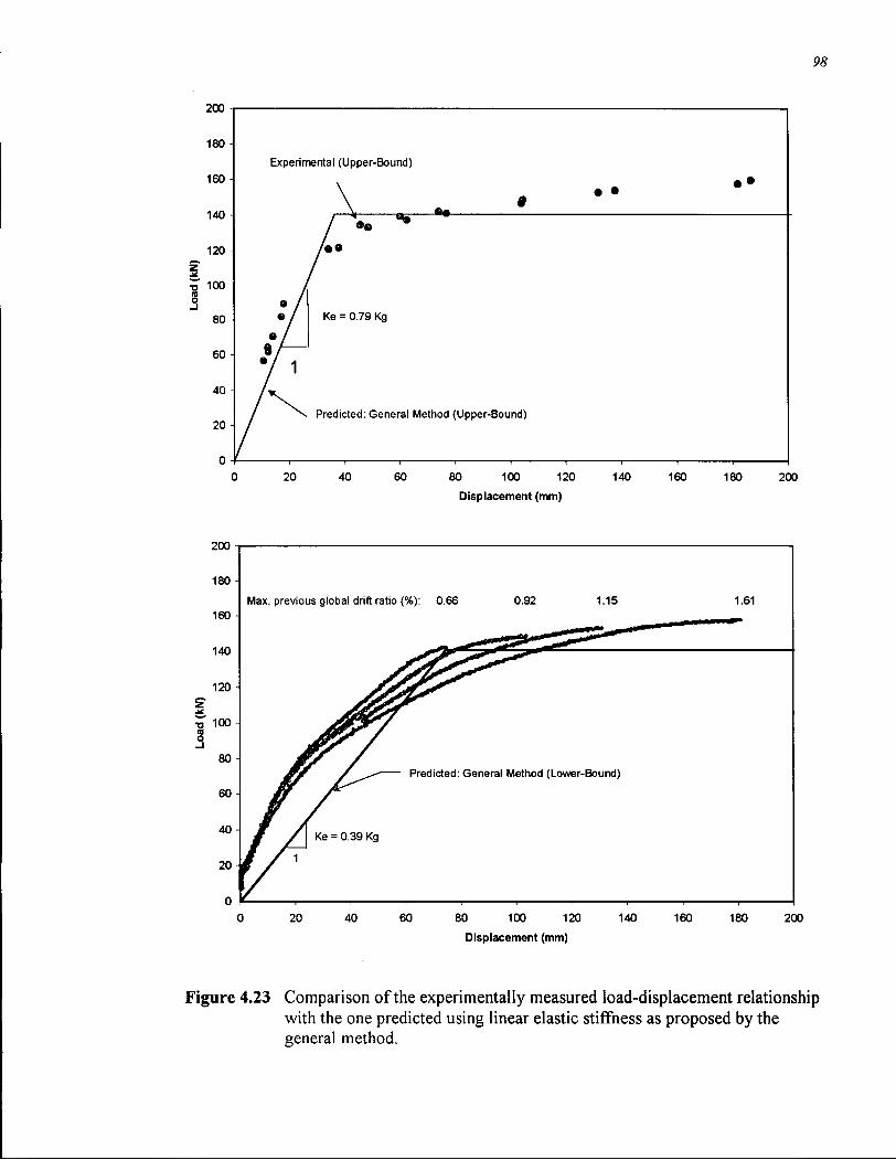
98
Figure 4.23 Comparison of the experimentally measured load-displacement relationship with the one predicted using linear elastic stiffness as proposed by the general method.

Figure 4.24 Comparison of the experimentally measured load-displacement relationship with the one predicted using the linear elastic stiffness suggested in the CPCA Handbook (1995).

100
200 j
180 -
200 Displacement (mm)
Figure 4.25 Comparison of the experimentally measured load-displacement relationship with the one predicted using the linear elastic stiffness suggested by the commentary to NZS 3101 (1995).

Chapter 5
Nonlinear Static Analysis of Concrete Walls
5.1 Introduction
One application of the proposed trilinear bending moment-curvature model is in nonlinear static
analysis procedure commonly known as pushover analysis or sequential yield analysis. Pushover
analysis is becoming increasingly popular and a necessary part of the design verification. It is
one of the three analysis methods recommended by the NEHRP Guidelines for Seismic
Rehabilitation of Existing Buildings (FEMA 273, 1997). It is also a main component in the
Capacity Spectrum method developed by Freeman et al (1975) and recommended by the Applied
Technology Council (ATC-40, 1996) to determine the displacement demand imposed on a
building that is expected to experience inelastic deformations.
The pushover analysis provides valuable insight into the performance of a structure under
earthquake loading, can be used to identify the weak elements in a structure, and to determine
inelastic rotation demands which are needed to assess the system ductility. A key component to
perform the pushover analysis procedure is the bending moment-curvature/rotation response of
the elements of a building (frame model, wall panels, etc.). Proper modeling of the material
properties is essential to obtain a useful result from the pushover analysis.
For a proper modeling of a wall element, and if the effect of cracking on the elastic deformations
of a wall structure is to be accurately modeled, the trilinear bending moment-curvature model
should be used. This flexural model, when combined with other models that capture the post-
yielding behavior (strain hardening-softening), shear failure mechanism, P-A effect, bond and
anchorage failure, etc., can provide a comprehensive representation of the structure performance
under the applied loading.
The pushover analysis, besides its advantages, does not seem to capture the displacements due to
higher modes of vibration, which are known to be of significance to the deflection of tall wall
101

102
structures. However, recent application of the pushover analysis to include the higher mode
effects has been developed and reported (Paret et al., 1996; Bracci et al., 1997).
In the following, an overview of the basic procedures used in the pushover analysis are
presented. Implementation of the trilinear model in a computer program to perform the
nonlinear static analysis is described. Necessary features required to perform the analysis and to
incorporate it into the computer program are also described. Finally, two example applications
of the model in analyzing a wall and a coupled wall structure are presented.
5.2 Overview of Pushover Analysis Procedure
The pushover analysis is a useful procedure to identify the weak links in the seismic performance
of a structure. A series of design iterations are usually carried out, during which the structural
deficiencies are observed and corrected (Naeim and Lobo, 1998). The iterative analysis and
design process continues until the design satisfies a pre-established performance criteria. The
performance criteria for the pushover analysis (as detailed in FEMA 274, 1997 and ATC-40,
1996) is generally established as the desired state of the building given the roof top displacement
(usually referred to as the target displacement).
The pushover analysis may be carried out using either force control or displacement control or a
combination of both. In force control analysis, the structure is subjected to an incremental
distribution of lateral forces to represent the seismic effects. In displacement control, the
structure is subjected to a prescribed displacement profile where the relative displacements of
key joints are constrained by simple geometric relationship. Since the deformed profile of
displacement is not easily defined, and a distributed load pattern to represent the seismic forces
are known and codified, force control is commonly used for building structures.
The analysis procedure usually involves modeling (subdividing) the structure into frame and
beam-like elements. The model is subjected to a lateral loading pattern such as a uniform
distribution, inverted triangular distribution, or fundamental mode of vibration (first mode)
distribution.

103
During a typical pushover analysis, the vertical (gravity) loads on the structure are held constant,
while the lateral loads are increased in small increments. At each load increment, the well
known system of simultaneous equations are assembled and solved:
K u = F [5.1]
Where K is the global stiffness matrix, u is the joint displacement and rotation vector, and F is
the applied load vector.
The vector of applied loads on each element is formed and assembled into the global load vector.
Both gravity and lateral loads are considered. The element stiffness matrix (function ofEJg) is
derived from the bending moment-curvature relationship defined for each element and then
assembled into the global stiffness matrix. Since the element end moments are not known yet,
the element stiffness matrix cannot be determined (i.e., K depends on u), the problem becomes
nonlinear and an initial guess for the element end moments are required in order to calculate the
stiffness.
Solution of this system of nonlinear equations requires an iterative scheme in which the initial
guess is refined and the stiffness is recalculated until the solution has converged arriving at the
correct stiffness values for each element. The analysis is continued for another load step
(increment) until the maximum (full) specified lateral load or the target displacement is reached,
or else the structure becomes unstable.
The correct element stiffness and end moments determine the state of cracking, yielding or
plastic hinge formation in each element at this load level. Inaccurate material modeling can lead
to an erroneous estimate of the structure performance.
When it is required to capture the strain hardening or softening characteristic of the building after
it reaches instability (i.e., formation of plastic hinges at all the supported nodes), the force
control is followed by a displacement control analysis provided that these effects are accounted
for in the material model.
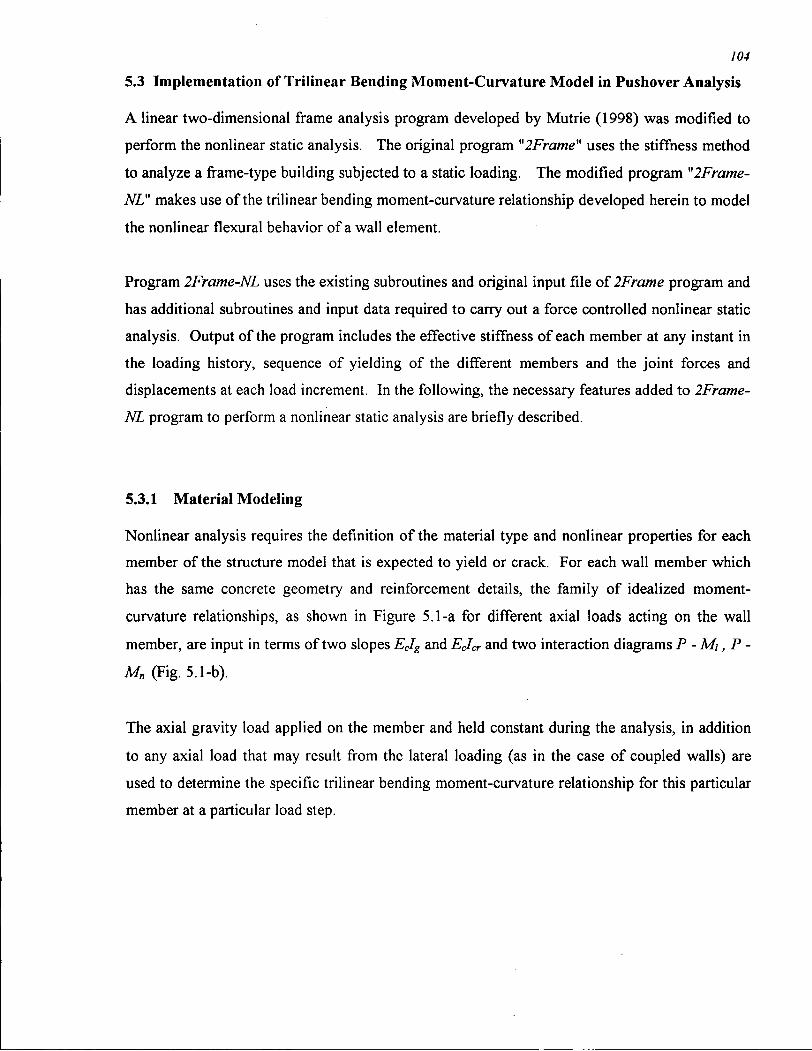
104
5.3 Implementation of Trilinear Bending Moment-Curvature Model in Pushover Analysis
A linear two-dimensional frame analysis program developed by Mutrie (1998) was modified to
perform the nonlinear static analysis. The original program "2Frame" uses the stiffness method
to analyze a frame-type building subjected to a static loading. The modified program "2Frame-
NL" makes use of the trilinear bending moment-curvature relationship developed herein to model
the nonlinear flexural behavior of a wall element.
Program 2Frame-NL uses the existing subroutines and original input file of 2Frame program and
has additional subroutines and input data required to carry out a force controlled nonlinear static
analysis. Output of the program includes the effective stiffness of each member at any instant in
the loading history, sequence of yielding of the different members and the joint forces and
displacements at each load increment. In the following, the necessary features added to 2Frame-
NL program to perform a nonlinear static analysis are briefly described.
5.3.1 Material Modeling
Nonlinear analysis requires the definition of the material type and nonlinear properties for each
member of the structure model that is expected to yield or crack. For each wall member which
has the same concrete geometry and reinforcement details, the family of idealized moment-
curvature relationships, as shown in Figure 5.1-a for different axial loads acting on the wall
member, are input in terms of two slopes EcIg and EcIcr and two interaction diagrams P - Mi, P-
Mn (Fig. 5.1-b).
The axial gravity load applied on the member and held constant during the analysis, in addition
to any axial load that may result from the lateral loading (as in the case of coupled walls) are
used to determine the specific trilinear bending moment-curvature relationship for this particular
member at a particular load step.
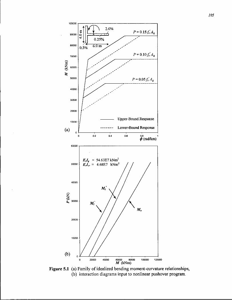
705
100000
90000
80000
70000
30000
20000
(a)
P = 0.15 fcAg
P = 0.10 fc'Ag
P = 0.05 fcAg
Upper-Bound Response
Lower-Bound Response
0.2 0.4 <p (rad/km)
30000
(b)
EJG = 54.63E7kNm2
EJCR = 4.68E7 kNm
20000 40000 60000 80000 100000 120000
M (kNm) Figure 5.1 (a) Family of idealized bending moment-curvature relationships,
(b) interaction diagrams input to nonlinear pushover program.

106
5.3.2 Determination of Effective Member Stiffness
During the iterative process to solve the system of nonlinear simultaneous equations, the
effective stiffness of each member is updated (re-calculated) whenever there is a change in the
end moments (i.e., nodal rotations). The effective stiffness is determined as follows (Figure
5.2): the bending moment distribution along the member length is determined from the member
end forces (assuming linear distribution between the two nodes); the trilinear bending moment-
curvature relationship, defined for each member as described above, is used to determine the
curvature distribution along the length of the member; the effective member stiffness EJe is that
which gives the equivalent rotation between the two ends of the member (i.e., equal area under
both actual and idealized linear curvature distributions).
The effective member stiffness EcIe is in general described as y/ EJg, where a new value of y/
cannot be taken greater than the y/max reached in the previous load increment. Figure 5.2 shows
the application of the above procedure on a typical wall segment for a general case of bending
moment distribution. Four cases are identified for the computation of the effective member
stiffness depending on the curvature distribution along the length of the member and are
illustrated in Appendix F.
The computational procedure to determine the effective member stiffness using the equal
rotation concept is also illustrated in Appendix F.
5.3.3 Solution of the Nonlinear Equations
Successive approximation technique (also known as direct iterations) is used to solve the system
of nonlinear simultaneous equations (Eq. [5.1]) during each load increment. Since the joint
displacements and rotations are not known at the first load increment, an initial estimate of the
stiffness is based on the gross section properties of each member. The system of equations are
then solved to obtain a set of values for joint displacements and rotations, and the end moments
for each member can then be computed from the basic principles of the stiffness method.
The computed end moments are used to determine the updated member stiffness matrix, as
described in the previous section, and thus the global stiffness matrix is updated (if necessary).

707
(a)
M i
Segment of wall
M 2
(b)
Bending Moment
M 2
M,
Curvature
(c)
Equivalent / linear
Actual
Uncracked
Figure 5.2 Application of trilinear bending moment-curvature model in non-linear static analysis: (a) bending moment distribution in a wall element, (b) trilinear bending moment-curvature model, (c) curvature distribution in a wall element.

108
The system of equations are solved again to obtain another set of values for the joint
displacements and rotations.
Figure 5.3 shows diagrammatically the iterative procedure for a single variable problem. The
iterative procedure is stopped or the solution has converged when a certain measure of the
change in the unknowns (end moments, member stiffnesses, or joint displacements and rotations)
between the successive iterations becomes less than a tolerable margin (acceptable level of
accuracy). The norm of the u vector is considered as the tolerance measure between the
successive iterations.
Care is taken regarding the convergence when using this iterative technique. The technique is
generally slower and less convergence when compared with other well-converged iterative
techniques such as Newton-Raphson, and Modified Newton-Raphson (Owen and Hinton 1980).
However, this technique is preferred in this course of work since it gives a meaningful member
stiffness (secant stiffness) at any particular instant of the analysis. This useful feature is
demonstrated later in the example applications (Figure 5.11). A simple technique used to ensure
the convergence between the successive iterations is to increase the number of loading steps (i.e.,
loading increments are decreased to about 5% of desired load).
5.3.4 Plastic Hinge Formation
A lumped plasticity approach was adopted to simulate the yielding of a wall element. This
approach assumes that yielding takes place only in concentrated plastic hinges located at the
element ends. When the bending moment at one end of a member reaches the yield (ultimate)
capacity defined in the bending moment-curvature relationship, a hinge is inserted in the
structure model and a joint moment is applied to simulate the plastic moment resisted by the
member.
[5.2]
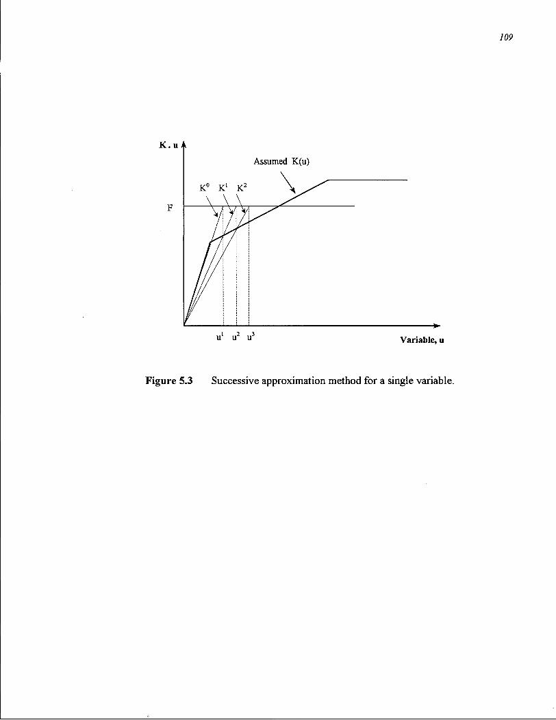
109
K . u A
Assumed K(u)
u1 u2 u3 Variable, u
Figure 5.3 Successive approximation method for a single variable.

110
Since the plasticity is lumped at a single joint and to enhance the accuracy of the modeling, care
needs to be taken when subdividing the structure so as to increase the number of members in the
region where plastic deformations may take place, usually at the base of the wall structure.
When all the members connected to the same joint reach the yield capacity, a single step
correction procedure is implemented to ensure the equilibrium of the joint.
5.4 Example Applications of the Pushover Analysis
Two examples are presented to demonstrate the application of the developed trilinear bending
moment-curvature model in predicting the flexural response of a wall structure using a static
pushover analysis. Program 2Frame-NL was used to perform the nonlinear static analysis for the
two examples.
In the first example, the load-displacement measurements taken from the wall test are compared
with the pushover analysis results predicted using the trilinear bending moment-curvature model.
In the second example, the pushover analysis is performed on a 32-story office tower with a
reinforced concrete coupled wall core system and the results are compared with the maximum
displacement demand on the structure. This example also serves to study the behavior (assess the
performance) of the coupled wall system when subjected to a simulated earthquake loading.
Results of the examples show the advantages of using the trilinear bending moment-curvature
model when predicting the flexural response of a wall structure over other models such as the
bilinear relation that is suggested by Priestley and Kowalsky (1998).
5.4.1 Wall Test Example
A static pushover analysis was carried out on the wall test specimen to predict the monotonic
load-displacement relationship. The wall test specimen was subjected to a constant axial
compression of 1500 kN. A single lateral load applied at the tip of the wall was used to apply a
reverse cyclic lateral displacement. Details of the specimen geometry and reinforcement were
given in Chapter 3.

Ill
The wall specimen was modeled as a cantilever stick and subdivided into members and joints.
The trilinear bending moment-curvature model used in the analysis for both the upper and lower-
bound response are shown in Figure 5.4. The analysis was run incrementally and the program
stopped when a plastic hinge formed at the base of the wall.
Figure 5.5 shows the computed load-displacement relation using the upper-bound trilinear
response. The measured upper-bound load-displacement response of the wall test is plotted on
the same figure for comparison. Also shown in the figure, is the load-displacement relation that
is predicted using the bending moment-curvature model suggested by Priestley and Kowalsky
1998. This prediction is based on a linear curvature distribution along the height of the wall and a
yield displacement of (0.33 <j>y H2) where the yield curvature is estimated as (2 ey / lw). The yield
strain, ey , of the 455 MPa reinforcing steel is equal to 0.00228. Note that this yield curvature
was originally suggested for rectangular wall shapes, whereas the wall test had flanged shape. It
is clear that the trilinear bending moment-curvature relationship describes the upper-bound
response of the wall test specimen much better than the Priestley and Kowalsky bilinear
relationship which is probably meant as a lower-bound response.
The pushover analysis was repeated for the wall test specimen using the predicted lower-bound
bending moment-curvature response. Figure 5.6 shows the predicted and experimental load-
displacement relationships. The experimental load-displacement relations are shown for only
the ascending ramp of the hysteresis loops for various displacement/drift levels. Each cycle is
labeled with the maximum drift ratio attained during the first cycle of loading. Because of the
observed degradation in stiffness from the first cycle to the second cycle, the second hysteresis
cycle for each drift level is the one shown in the figure as was done in Chapter 4.
The global drift shown in the figure is computed similar to the procedure outlined in Chapter 4.
The local drift ratio was estimated as the sum of the elastic drift (1.5*Ay / H) and plastic drift ({A
- A y }/ H) at each load level, where H is the height of the wall and A y is the yield displacement
computed from the measured monotonic response and found to be 33 mm. The displacement
ductility estimated for each load cycle is also shown on Figure 5.6. The displacement ductility
was computed as the maximum displacement reached at each cycle divided by the estimated
yield displacement.

Figure 5.4 Trilinear bending moment-curvature relationship used for the analysis of the slender wall specimen.
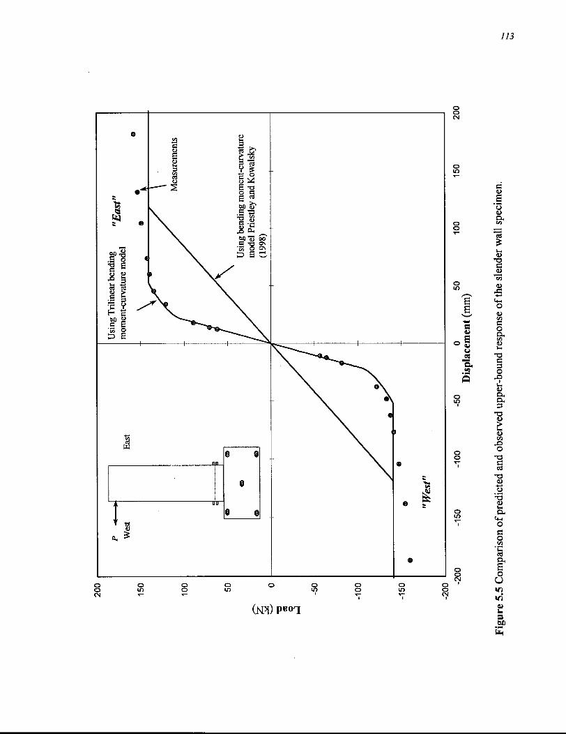
113

114
Figure 5.6 Comparison of predicted and observed lower-bound response of the slender wall specimen.

115
It is seen that the lower-bound trilinear bending moment-curvature model predicted a reasonable
lower-bound estimate of the load-displacement relation. The load-displacement relation
predicted using the Priestley and Kowalsky bilinear model significantly over-estimates the
elastic deflections.
5.4.2 Coupled Wall Example
A coupled wall structure example is presented to illustrate the use of the trilinear bending
moment-curvature model in determining the elastic deformations of wall members. The example
was done as part of the design of Lincoln Square, a 1.6 million square ft development in the City
of Bellevue, Washington. The objective was to better understand the behavior of a coupled
wall structure when subjected to an incremental loading (by means of a static inelastic analysis)
in addition to evaluating the system performance under a given maximum displacement demand.
Description of the project example:
The core wall structure is a 32-story office tower with an overall height of 450 ft above grade.
Figure 5.7-a shows a three dimensional isometric view of the coupled wall core. Details of the
cross section geometry are shown in Figure 5.7-b.
The core structure was analyzed in the long (coupled) direction. Additional openings were
subsequently added to make the core coupled in the short-direction as well (Mutrie et al., 2000),
but these are of no interest in this two-dimensional example. The example shown here is for the
east-west direction only despite the unsymmetrical shape of the cross section.
The two-dimensional model of the structure in the long direction is shown in Figure 5.8. The
four walls were modeled as column-like members located at the gross section centroid. The
coupling beams were modeled as a beam-like elements connected to the columns using infinite
stiffness extensions (rigid links). The nodes (joints) at each floor level were constrained to have
the same horizontal displacement simulating rigid diaphragm action.
Prior to undertaking the two-dimensional nonlinear static analysis, a three-dimensional linear
dynamic analysis of the structure was done by others (Adebar et al., 1999) to determine the first
mode distribution of forces and the shear demand on the coupling beams; as shown qualitatively
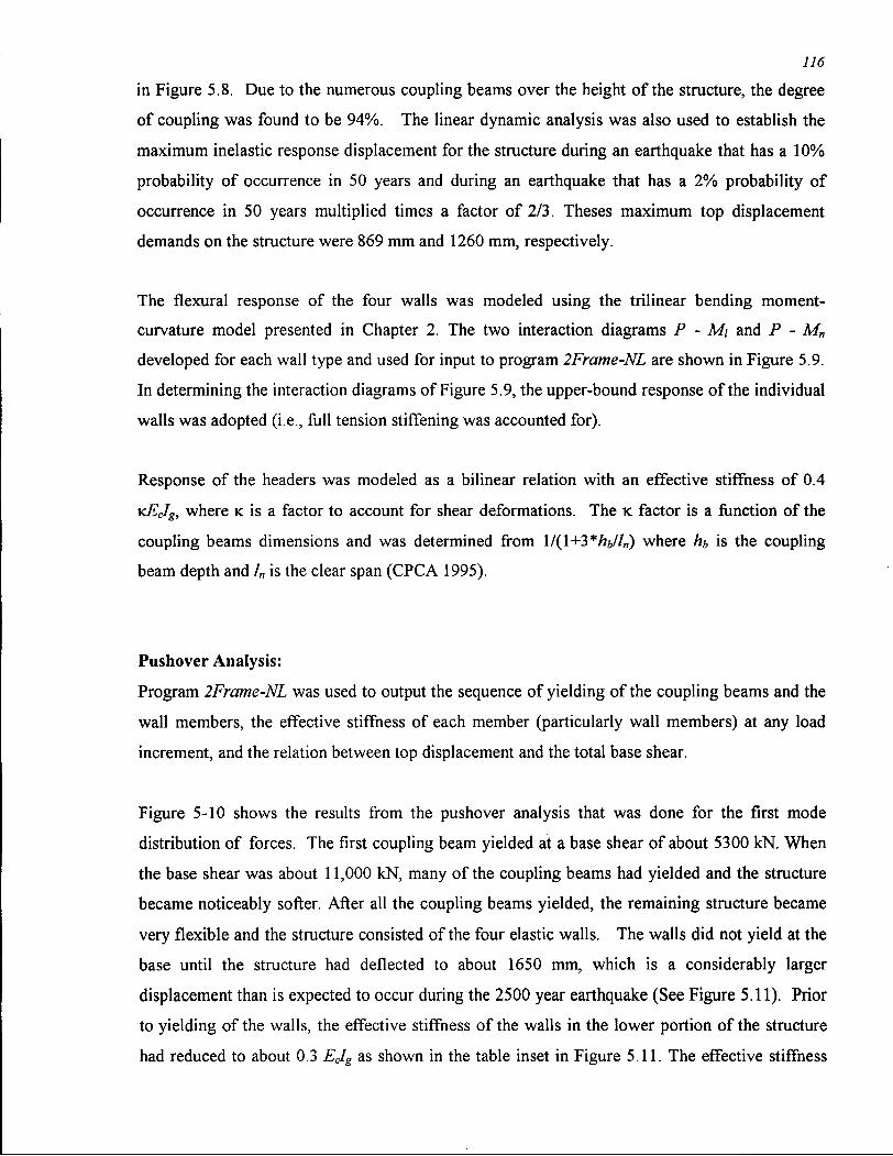
116
in Figure 5.8. Due to the numerous coupling beams over the height of the structure, the degree
of coupling was found to be 94%. The linear dynamic analysis was also used to establish the
maximum inelastic response displacement for the structure during an earthquake that has a 10%
probability of occurrence in 50 years and during an earthquake that has a 2% probability of
occurrence in 50 years multiplied times a factor of 2/3. Theses maximum top displacement
demands on the structure were 869 mm and 1260 mm, respectively.
The flexural response of the four walls was modeled using the trilinear bending moment-
curvature model presented in Chapter 2. The two interaction diagrams P - Mi and P - M„
developed for each wall type and used for input to program 2Frame-NL are shown in Figure 5.9.
In determining the interaction diagrams of Figure 5.9, the upper-bound response of the individual
walls was adopted (i.e., full tension stiffening was accounted for).
Response of the headers was modeled as a bilinear relation with an effective stiffness of 0.4
KEcIg, where K is a factor to account for shear deformations. The K factor is a function of the
coupling beams dimensions and was determined from 1/(1+3 */»&//„) where hf, is the coupling
beam depth and /„ is the clear span (CPCA 1995).
Pushover Analysis:
Program 2Frame-NL was used to output the sequence of yielding of the coupling beams and the
wall members, the effective stiffness of each member (particularly wall members) at any load
increment, and the relation between top displacement and the total base shear.
Figure 5-10 shows the results from the pushover analysis that was done for the first mode
distribution of forces. The first coupling beam yielded at a base shear of about 5300 kN. When
the base shear was about 11,000 kN, many of the coupling beams had yielded and the structure
became noticeably softer. After all the coupling beams yielded, the remaining structure became
very flexible and the structure consisted of the four elastic walls. The walls did not yield at the
base until the structure had deflected to about 1650 mm, which is a considerably larger
displacement than is expected to occur during the 2500 year earthquake (See Figure 5.11). Prior
to yielding of the walls, the effective stiffness of the walls in the lower portion of the structure
had reduced to about 0.3 EJg as shown in the table inset in Figure 5.11. The effective stiffness

Figure 5.7 (a) Isometric view of the core wall example, (b) cross section dimensions (3.28 ft = 1 m).

118
(a)
•
(b)
Header capacity
/ Elastic header
^ demand
Figure 5.8 (a) two-dimensional plane frame model subjected to first mode loading, (b) coupling beam shear capacity and demand.

119
P(kN) 120000
10--4"
fc = 30 MPa fy = 400 MPa
-200000 -150000 -100000 -50000 0 50000 100000 150000 200000 250000
M (kNm)
P(kN) —120000
100000 H
80000
60000
40000 H
20000 i
fc = 30 MPa fy = 400 MPa
M +
18"
-200000 -150000 -100000 -50000 0 50000 100000 150000 200000 250000 300000
M (kNm)
Figure 5.9 Interaction diagrams for the four core walls and used for input to the pushover analysis.

120
results shown in this table pertains to the wall with the least compression in the core
configuration (the first wall from the left side). Note that this degradation of stiffness in the
lower portion of the wall is not detected if using a simple bilinear model with one constant
effective stiffness prior to yielding.
As seen from the results in Figure 5-11, the highly coupled wall system dissipated the energy of
the applied loading by yielding of the coupling beams and the walls remained elastic for a
considerable displacement afterwards. Thus, it is of great importance to accurately model the
flexural deformations of the wall members within the elastic range.
In addition to illustrating the importance of modeling the elastic deformations of the wall
structure, the results of the example also provide useful insight into the behavior of the highly
coupled core wall system. It is usually conservative to assume a lower than actual stiffness, as
the displacement demand is correspondingly increased. However, assuming lower than actual (or
alternatively, the lower-bound rather than the upper-bound) flexural stiffness of the individual
walls in this case does not significantly influence the initial stiffness of the highly coupled wall
system but rather results in unconservative larger elastic deflections prior to yielding of the walls
and smaller inelastic demands on the walls.
The analysis indicated that the wall elements yielded approximately at the same time step. As
soon as any particular wall began to yield, a mechanism started and the shear force demand
increased significantly on the other wall elements leading eventually to their yielding.
The highly coupled core wall system is a highly desirable system for resisting earthquake loading
in high-rise buildings. In the example shown, walls with minimum reinforcement amount
remained elastic during a 2500 yr. earthquake. It is very desirable to have a system in which the
gravity load resisting elements remain elastic.
The pushover results shown in this example did not consider the contribution of higher modes to
the deflection of this tall core wall structure. Since the interest is to assess the ductility of such
systems and as the maximum displacement demand on the structure will be first mode
dominated, this analysis seems appropriate.

121
Figure 5.10 Sequence of yielding of the different members in the two-dimensional frame model.

122
16000
0 - f 1 > 1 1 1 1 — • 1 1 1 1 0 200 400 600 800 1000 1200 1400 1600 1800 2000
Top Displacement (mm)
Figure 5.11 Predicted nonlinear static response of 450 ft high coupled walls.

Chapter 6
Conclusions and Recommendations
6.1 Summary and Conclusions
In the seismic design of high-rise wall buildings, the fundamental period of the building (which
influences the design base shear) and the building drift are usually determined using linear
dynamic analysis. To carry out the analysis, designers need to use an effective flexural stiffness
of the wall sections that accounts for the effects of cracking. The effective stiffness
recommendations from different design guidelines vary by about a factor of three and it is not
clear which stiffness value should be used for any particular wall.
The nonlinear static analysis method can be used to assess the inelastic deformations that are
expected to occur in walls and coupled wall systems, but requires an appropriate material model
in order to yield useful results. While plane sections computer models that can predict the full
nonlinear response of wall sections commonly exist, using such a complex material model would
add an unnecessary degree of complexity to the analysis. One of the main advantages of the
nonlinear static method is the transparency of the procedure. Most nonlinear static analysis is
currently done using a simple bilinear (elastic-plastic) model for concrete walls. Thus what is
needed is a simple piece-wise linear model that properly accounts for the effect of cracking.
The inconsistency in the recommended stiffness for linear seismic analysis and the need for a
simple nonlinear model for nonlinear seismic analysis of concrete walls prompted the following
contributions made in this thesis.
A study of the bending moment - curvature response of concrete walls with significant axial
compression and low amounts of vertical reinforcement (typical in high-rise walls) indicated that
the elastic deformations are not appropriately represented by a simple bilinear idealization. In
particular, a bilinear relationship with the linear stiffness defined as the capacity divided by the
yield curvature greatly underestimates the effective stiffness. The bending moment - curvature
relationship for concrete walls can be better approximated using a trilinear model.
123
124
In Chapter 2 of this thesis, a trilinear bending moment curvature model for the flexural response
of concrete walls was introduced. In order to capture the effect of cracking on the flexural
stiffness of concrete walls in a simple transparent way, the elastic portion of the bending moment
- curvature relationship was modeled as bilinear. The model accounts for the influence of cyclic
loading on tension stiffening of the cracked concrete by introducing the concept of upper-bound
response for a previously uncracked wall and lower-bound response for a severely cracked wall.
The trilinear model is defined by four parameters: the slope of the initial linear response EcIg,
the slope of the second linear segment EcIcr, the bending moment defining the intersection of the
first and second linear segments, Mi, and the flexural capacity M„. Two of these parameters EcIg
and M„ are well known to designers and can easily be determined by hand calculation. The third
parameter Ec Icr is also well known, but is very difficult to determine by hand calculation for
typical wall sections with distributed vertical reinforcement. Thus design charts were developed
as part of this thesis. Finally, an equation was developed to permit the easy calculation of the
fourth parameter Mi. It is this parameter that accounts for the difference between the upper-
bound and lower-bound response that captures the effect of cyclic loading. The proposed
trilinear bending moment - curvature model can easily be incorporated into a nonlinear static
analysis program for concrete walls (as was done in Chapter 5), or can be used as the foundation
of a general rational model for determining the effective linear stiffness of concrete walls (as was
done in Chapter 4).
A large-scale test was conducted on an approximately quarter-scale model of a slender wall.
Based on the results of a literature search, it appears that this is the most slender wall ever tested.
The specimen was 40 ft "high" and 5.3 ft long, which corresponds to a height-to-length ratio of
7.5. The purpose of the test was to observe the response of a slender wall with a low percentage
of vertical reinforcement and subjected to significant axial compression, and to obtain the
information needed to validate the proposed trilinear bending moment - curvature model.
The observed initial stiffness of the concrete wall corresponded reasonably well to the predicted
uncracked gross section stiffness EcIg. When the wall was reloaded after having been
significantly cracked, the initial stiffness was again approximately equal to the uncracked section
stiffness EJg due to the axial compression closing the cracks when the bending moment was
removed. As predicted by the proposed model, the extent of the initial linear range, i.e., Mi,

125
reduced after the wall was cracked. The predicted lower-bound response corresponded
reasonably well to the response of the wall after it had been subjected to global drift levels of
about 1.5%. The experimentally measured relationship between curvature and the corresponding
applied bending moment were found to agree well with the predicted relationship.
The trilinear bending moment - curvature model, having been calibrated to the results of the
large-scale wall test, was used to develop a general, consistent method to predict the effective
(linear) flexural stiffness of concrete walls. To account for the degradation of stiffness during
the cyclic motion of an earthquake, the effective stiffness of concrete walls was considered to
range from an upper-bound effective stiffness to a lower-bound effective stiffness. The general
method uses the two non-dimensional parameters that describe the bending moment - curvature
relationship of the cross section at the base of the wall: the ratio of the cracked section moment
of inertia to the uncracked section (gross) moment of inertia Icr I Ig, and the ratio of the linear
bending moment to the capacity of the wall section at the base Mi / M„.
The general method was used to study the influence of a variety of parameters on the effective
stiffness of concrete walls. The results of the study indicate that the effective flexural stiffness of
concrete walls can vary from as little as 0.1 Ig to as high as 1.0 Ig depending on: state of cracking,
magnitude of axial compression, geometry of the wall cross section, amount of vertical
reinforcement, yield strength of the vertical reinforcement and concrete compressive strength.
Thus, the very large variation in effective stiffness that is seen in various design guidelines does
actually exist, and each guideline is correct for certain types of walls under certain conditions.
The general method presented in this thesis is the only method that accounts for all the
parameters and gives the appropriate stiffness for a particular wall.
Based on the general method for determining the effective flexural stiffness of concrete walls, a
set of simplified expressions for the upper-bound and lower-bound effective stiffness was
proposed. The simplified expressions capture the influence of several parameters that affect the
stiffness in an approximate way and are particularly useful in the initial stages of design when
the concrete geometry has not been finalized and the amount of reinforcement is not known.
The upper-bound effective flexural stiffness can be used in a force-based design where engineers
start the design process by estimating the fundamental period of the building and the

126
corresponding design accelerations and forces. The upper-bound stiffness is used to get a lower-
bound estimate of the period and thus a higher estimate of the design forces and seismic actions.
In a displacement-based design, where the displacement is the major concern, designers should
estimate the period and the corresponding displacements using the lower-bound effective
stiffness.
The proposed trilinear bending moment - curvature model was implemented into a nonlinear
static analysis program. Numerical techniques used to implement the trilinear model were
presented in Chapter 5. The nonlinear static analysis program was used to demonstrate the use
and advantages of the proposed model over other suggested models through two example
applications. Further validation of the proposed trilinear model was illustrated in the first
example where the predicted load-deformation relationship for the slender wall test compared
well with the measured response of the wall. The nonlinear static response of a high-rise
coupled wall system was presented in the second example. The nonlinear static analysis was
used to assess the ductility of a coupled wall core system that is currently being constructed near
the city of Seattle, Washington. Results from the example showed the importance of accurately
modeling the elastic deformations of concrete walls using the proposed trilinear model and
provided useful insight into the behavior of such highly coupled wall systems.
6.2 Recommendations for Further Work
The proposed trilinear bending moment - curvature model assumes no increase in the capacity of
the wall after all the vertical reinforcement has yielded. As seen from the slender wall test, a
significant increase in the bending moment capacity is possible at very large drift ratios. For
simplicity, strain hardening of the reinforcement was ignored in the proposed trilinear
relationship. The third linear segment in the bending moment - curvature relationship could be
inclined at a certain slope to account for strain hardening. However, as the strain hardening
characteristics vary significantly for different types of reinforcing steel, it is difficult to define
such a slope in the same generic way as has been done for the other elements of the proposed
trilinear model.
While the majority of concrete walls and coupled walls in high-rise buildings are subjected to
significant axial compression, there are cases where the wall segment of a coupled wall system

127
may be subjected to axial tension, particularly in medium to low rise buildings. As the lateral
earthquake displacements are increased, the coupling beams yield sequentially creating a
gradually increasing compression force in one wall and tension force in the other wall. The
tension force due to the coupling beam shears can offset the initial axial compression due to
gravity loads and result in a net tension force being applied to the wall segment. The proposed
trilinear bending moment - curvature relationship is not appropriate when the axial tension
applied to a wall section causes the entire wall section to be subjected to vertical tension strains.
Additional work needs to be done to develop an appropriate model for this condition.
The proposed trilinear model represents the loading portion of the full cyclic bending moment -
curvature response (hysteresis loop) of a concrete wall. The loading portion of the response is
precisely what is needed for a nonlinear static analysis. To perform a nonlinear dynamic
analysis, however, a full hysteresis model is needed. It is proposed that the trilinear bending
moment - curvature relationship be used as the basis of a hysteretic model for concrete walls in
high-rise buildings, and that the experimental results from the slender wall test be used to
calibrate such a model.
References
Abrams, D. P. (1991), "Laboratory definitions of behavior for structural components and building system," ACI SP-127, Vol. 127,no. 4,pp. 91-152, Aprill991.
Adebar, P., and Ibrahim, A.M.M. (2000), "Simple non-linear flexural stiffness model for concrete shear walls," Earthquake Spectra, EERI, In press.
Adebar, P., Ibrahim, A.M.M., and Bryson, M. (2000), "Large-scale test of a slender concrete shear wall," Report, Department of Civil Engineering, University of British Columbia, 210 pp.
Adebar, P., Mutrie, J.G., and Ibrahim, A.M.M. (1999), "Inelastic static analysis to evaluate the ductility of coupled walls in a tall building," 8th Canadian Conference on Earthquake Engineering, Vancouver, BC, pp. 421-426.
Applied Technology Council (1996), "Seismic evaluation and retrofit of concrete buildings," Report ATC 40, Applied Technology Council, Paio Alto, California.
Bracci, J.M., Kunnath, S.K., and Reinhorn, A. M. (1997), "Seismic performance and retrofit evaluation of reinforced concrete structures," Journal of Structural Engineering, ASCE, 123, 3-10.
Bryson, M. (2000), "Testing of the lateral stiffness of a lender concrete shear wall," CIVL 598 Directed Studies Report, Department of Civil Engineering, The University of British Columbia, pp. 162.
Charney, F.A. (1991), "Correlation of the analytical and experimental inelastic response of a 1/5 scale seven-story reinforced concrete frame-wall structure," ACI SP-127, pp. 261-361.
Chopra, A.K. (1995), "Dynamics of structures: Theory and applications to earthquake engineering," Prentice Hall, New Jersey.
Collins, M.P., and Mitchell, D. (1991), "Prestressed concrete structures," Prentice Hall, 766 pp.
Council on Tall Buildings and Urban Habitat (1992), "Cast-in-place concrete in tall building design and construction," McGraw-Hill.
CPCA (1995) Explanatory notes on CSA standard A23.3-94, Concrete design handbook, 2nd ed., Ontario, Canada.
CSA (1994), "Design of concrete structures," CSA Standard A23.3-94, Canadian Standards Associations, Rexdale, Ontario, 199 pp.
FEMA 273 (1997), "NEHRP Guidelines for the seismic rehabilitation of buildings," Federal Emergency Management Agency, Washington, D. C.
128
129
FEMA 274 (1997), "NEHRP Commentary on the guidelines for the seismic rehabilitation of buildings," Federal Emergency Management Agency, Washington, D. C.
Fintel M. (1991), " Shearwalls - an answer for seismic resistance?", Concrete International, Vol. 13, No. 7, pp. 48-53.
Freeman, S. A., Nicoletti, J.P., and Tyrell, J.V. (1975), "Evaluations of existing buildings for seismic risk - A case study of Puget sound naval shipyard," Bremerton, Washington, Proceedings of 1st U.S. National Conference on Earthquake Engineering, EERI, Berkeley, 113-122.
French, C.W., and Schultz, A.E. (1991), "Minimum available deformation capacity of reinforced concrete beams," ACI SP-127, pp. 363-419.
Fronteddu, L. (1993), "Response of reinforced concrete to reverse cyclic loading," M.A.Sc. Thesis, Department of Civil Engineering, The University of British Columbia.
Fronteddu, L., and Adebar, P. (1992), "Response of structural concrete to axial tension," Proceedings of the Annual CSCE Conference, Vol. IV, Quebec City, pp. 89-98.
Ibrahim, A.M.M., and Adebar, P. (2000), "Effective flexural stiffness of concrete shear walls," Journal of Structural Engineering, ASCE, In press.
Meigs, B. E., Eberhard, M. O., and Garcia, L. E. (1993), "Earthquake-resistant systems for reinforced concrete buildings: a survey of current practice," Report no. sgem 93-3, Department of Civil Engineering, University of Washington, Seattle.
Mutrie, J.G., Adebar, P., and Leung, K. (2000), "Design of high-rise concrete shear wall buildings: Canadian vs. U.S. practice," Proceedings of SEAOC Convention, Vancouver, B.C., Aug. pp. 169-179.
Mutrie, J.G. (1998), " Program 2Frame, In-House program for plane frame analysis of buildings," Jones Kowng Kishi, North Vancouver, Private communication.
Naeim, F., and Lobo, R.F. (1998), "The ten commandments of push-over analysis," Proceedings of the 1998 annual meeting, Los Angeles Tall Buildings Structural Design Council, Los Angeles, CA.
NZS 3101 (1995) Commentary on the design of concrete structures, Standard New Zealand, New Zealand.
Owen, D.R.G., and Hinton, E. (1980), "Finite elements in plasticity: theory and practice," Pineridge Press, Swansea, U.K.
Paret, T. F., Sasaki, K. K , Eilbekc, D.H., and Freeman, S.A. (1996), "Approximate inelastic procedures to identify failure mechanisms from higher mode effects," Paper no. 966, 11th World Conference on Earthquake Engineering, Acapulco, Mexico.

130
Park, R., and Paulay, T. (1975), "Reinforced concert structures," John Wiley and sons, New York.
Paulay, T. (1997), "Seismic torsional effects on ductile structural wall systems," Journal of Earthquake Engineering, Vol. 1, No. 4, pp. 721-745.
Paulay, T., and Priestley, M. J. N. (1992), "Seismic design of reinforced concrete and masonry buildings," John Wiley and sons, New York, 744 pp.
Priestley, M. J. N. (2000), "Performance Based Seismic Design," Paper no. 2831, 12th World Conference on Earthquake Engineering, Auckland, New Zealand.
Priestley, M. J. N , and Hart, G. C. (1989), "Design recommendations for the period of vibration of masonry wall buildings," Research Report SSRP 89/05, University of California, San Diego and Los Angeles, 46 pp.
Priestley, M.J.N., and Kowalsky, M.J. (1998), "Aspects of drift and ductility capacity of rectangular cantilever structural walls," Bulletin of the New Zealand National Society for Earthquake Engineering , Vol. 31, No. 2, pp. 73-85.
Saatcioglu, M. (1991) "modeling hyestertic force deformation relationship for reinforced concrete elements," ACI Sp-127, pp. 153-198.
Saatcioglu M., and Bruneau M. (1993), "Performance of structures during the 1992 Erzincan earthquake," Canadian Journal of Civil Engineering, 20, pp. 305-325.
SEAOC 1996. Seismology committee, Structural Engineers Associations of California (SEAOC), "Recommended lateral force requirements and commentary".
Thomsen IV, J.H., and Wallace, J. W. (1995), "Displacement-based design of RC structural walls: an experimental investigation of walls with rectangular and T-shaped cross sections," Report No. CU/CEE-95/06, Department of Civil and Environmental Engineering, Clarkson University, Potsdam, New York.
Veechio, F.J. (1999), "Towards cyclic load modeling of reinforced concrete," ACI Structural Journal, Vol. 96, pp. 193-202.
Veechio F. and Collins M.P. (1986), "The modified-field compression theory for reinforced concrete elements subjected to shear", ACI Journal, Vol. 83, No. 2, pp. 219-231.
Wallace, J. W., and Moehle, J. P. (1992), "Ductility and detailing requirements of bearing wall buildings," Journal of Structural Engineering, ASCE, Vol. 118, No. 6, pp. 1625-1644.
UBC 1997. Uniform Building Code, International conference of building officials, Whittier, California.

Appendix A
Plane Sections Analysis Procedure
Determination of the actual nonlinear bending moment-curvature relationship is done using
plane sections analysis that satisfies the equilibrium of forces, strain compatibility and the stress-
strain relationships. The analysis procedure assumes linear strain distribution along the wall
cross section; and that the stress-strain relationship for concrete and steel are known.
The stress-strain relationship for concrete in compression and for steel in tension and
compression used in this work are shown in Figure A. l . The stress-strain relationship for
concrete in tension was illustrated in Chapter 2 (Figure 2.5).
Linear strain distribution along the cross section is defined by two variables, for instance, strain
at centroid and strain gradient (curvature). If the strain distribution is known or assumed, then the
stress-strain relationships for concrete and steel can be used to find the distribution of stresses
along the section. Knowing the stresses, bending moment and axial capacities of the cross
section can be determined from the following equilibrium equations.
P = \ fcdA c + j fsdA s
Ac A s
-M = j fcydAc + j fsydAs
A c A s
These equilibrium equations involve performing the integration over the area of cross section.
Since the strain distribution is non uniform across the depth of the wall, evaluation of these
integrals is not a straightforward task. One convenient procedure to evaluate these integrals is to
idealize the wall cross section as a series of rectangular layers and to assume uniform strain in
each layer. If the strain is uniform within a layer, then the stress within the layer is also uniform.
The equilibrium integrals then become a matter of multiplication of area of each layer times the
corresponding uniform stress. Figure A.2 summarizes the layered approach to solve the
equilibrium equations.
131

To determine the bending moment at a given curvature, the strain distribution across the wall
section must be determined so as to satisfy the equilibrium equations. Commonly, axial load is
known providing one condition of equilibrium. For a given/assumed curvature, a trial value of
strain at a given reference is assumed (strain at centroid for example) and an iterative technique
is performed to satisfy the known axial load. Once this condition is satisfied, strain distribution
across the wall section is thus known and the corresponding bending moment is determined from
the second equilibrium equation.
132

fc
t/3
(a)
±fy
(b)
Strain, £
Es =j= 200,000 MPa
Strain, £ s
Figure A . l Stress-strain relationship for a) concrete in compression, b) steel in compression and tension.
LS2 ES1
(a) Layered Cb) Concrete (c) Steel (d) Concrete stresses (e) Steel CO Stress cross section strains strains and forces forces resultants \
Figure A.2 Evaluating equilibrium equations using layer by layer procedure (from Collins and Mitchell, 1991)
133

Appendix B
Bending Moment-Curvature Relationship
Considering Residual Strains due to Cyclic Loading
The bending moment-curvature relationships shown previously in Figure 2.7, were predicted
ignoring the effect of residual strains due to cyclic loading as the influence of these were
assumed to be small. In the following, the bending moment-curvature relationships for the same
wall configuration are repeated considering the effect of residual compressive strains in concrete
and residual tension and compression strains in reinforcement.
Figure B.l-a shows the bending moment-curvature relationships considering the cyclic response
of concrete in tension (as explained previously in section 2.5) and residual strains in concrete and
reinforcement. The stress-strain relationship for concrete in compression was assumed to unload
and reload to the envelope of the monotonic relationship parallel to the initial gross stiffness
resulting in residual compressive strains at zero stress (Fig. B.l-b). The stress-strain-relationship
for the reinforcement was assumed bilinear. Unloading and reloading to an increased
deformation follow the same initial linear slope resulting in residual strains at zero stress (Fig.
B.l-c). Note that the lower-bound bending moment-curvature relationship shown in the figure
was assumed to reach the strain at peak stress (ec
f = 0.0033 for fc =50 MPa).
As shown in the figure, the resulting loading curves are only slightly offset from the origin
particularly during the early cycles. This small offset is attributed to the concrete compressive
stresses being predominately linear prior to yielding of the reinforcement. The offset, however,
can be of significance when the concrete reaches high values of compressive strains particularly
for cycles with large drift ratios and when the reinforcement yields to large strain values. The
experimental results, shown in Figure 3.11, indicate that the offset is relatively small in the range
of expected drift/ductility.
134

120000
0.1 0.2 0.3 0.4
Curvature (rad/km)
Concrete in compression Steel in tension
0.003 0.004
Strain Ec = 0.0037
•< >•
Curvature (rad/km)
4>a=0.2
<|>b=0.4
•c=0.7
Max. compressive strain previously reached:
sA = -0.00061
e b = -0.0008
e c = -0.0011
Figure B. l Bending moment-curvature relationships considering residual strains due to cyclic loading.
135
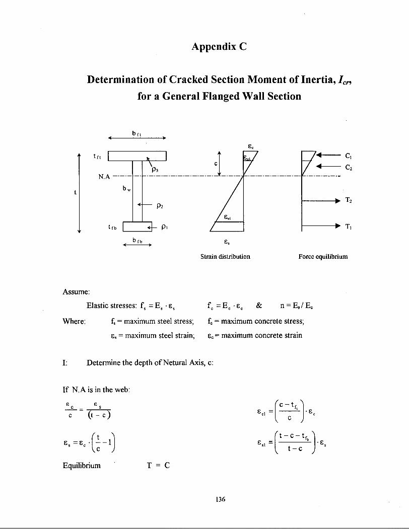
Appendix C
Determination of Cracked Section Moment of Inertia, It
for a General Flanged Wall Section
t
Strain distribution Force equilibrium
Assume:
Elastic stresses: fs = E s • ss f c = E c - e c & n = E 9 / E c
Where: fs = maximum steel stress; fc = maximum concrete stress;
ss = maximum steel strain; ec = maximum concrete strain
I: Determine the depth of Netural Axis, c:
If N. A is in the web:
e e
c _ s
c ( t - c )
e s=e c- —1 Equilibrium T = C
t - c - t f
I t - c J
136

• T ,=E S
V ^ J
where = E
tfb -bfb -Pi
t - c - ( t f b / 2 )
\ ^ J -1
• T 2 = E S ( t - c - t f b ) - b w -p 2
\^ J
b f t - t f t
• C 2 = E C (c-t f l )-b,
E E s c
E -8 c c
t-c-(t f b /2)"
C, +C 2 =T, +T2
t f b -b f b -P, +E S
t - c - t fb
= "(tft/2)" • b f t - t f t + E c - ^ . c- t ,
( t - c - t f b ) b w -p 2
t - c •(tfb/2)" c
(tft/2)"
tfb -b f b -P, +• t - c - t fb ( t - c - t f b ) - b w -p 2 =
b f t - t f t + E c - - -c - t ft ( c -t f ,)-b v
2n ftfb ftfb t -
ftfb - c I 2 )
t f b • b f b • P, + n • [t - t f b - c]- (t - t f b -c) -b w • p.
2-[c-(t f t /2)] .b f l -t f t +[c-t f t ]-(c-t f i ) .b,
n [ t - t f b - c ] 2 b w p 2 + [ c - t j 2 - b w + 2 n -
-2.[c-(t f b /2)]-b f l -t f t =0.0
t -lfb t f b -b f b -p,
n-p 2 -b w -[(t-t f b) 2 -2-( t - t f b ) -c + c 2 ] - b w [c2 - 2-c-t f t +t f t
2]+
2-n-p, -t f b -b f b - [ t - (t f b /2)-c]-2.t f t -b f t -[c-t fb/l]=0.0
Quadratic Equation in c: X-c2 + Y-c + Z = 0
137

Where:
X . c 2 =
Y. c =
Z =
Then,
X:
Y:
Z:
n . p 2 . b w . c 2 - b w - c 2
- 2 - n - p 2 - b w - ( t - t f b ) - c + 2 - b w - t f t - c -2 -n-p, -t f b -b f b - c -2 - t f t -b f t -c
n-p 2 -b w - ( t - t f b ) 2 - b w - t f t
2 + 2 -n -p , - t f b -b f b - ( t - t f b / 2 )+2 . t f t -b f t / 2
( n p 2 - l ) b w
- 2 - n - p 2 - b w • ( t - t f b ) + 2 - b w - t f t - 2 . n . p 1 . A f b - 2 - A f t
n-p 2 -b w - ( t - t f b ) 2 - b w - t f t
2 +2-n-p, - A f b • ( t - t f b 12)+ A f t -t f b
/ 2_ Solution of the quadratic equation : ~ Y ± V Y ~ 4 X Z gives the neutral axis depth, c.
2 * X
II: Determine the moment of inertia, Icr, from the parallel axis theorem:
I « = -b....c-
l - ^ f r ' f t c -• + n . P l . t f b . b f b t - t f b / 2 - c + n. P 2 - t - c - t fb
Note that if the N . A depth, c, lies in the flanges, the equilibrium equation need to be resolved for the new conditions.
138

Appendix D
Determination of Linear Bending Moment, M\ i
The three parameters: EJg, EcIcr, M„ should be pre-calculated in order to determine the linear
bending moment, Mi.
M (j, = n
N E I c cr
M_ - M , <|> =4.+—2 1 v y V l E I c cr
•1 = M,
E I c g
Area = J^" M d<J> Area °f actual nonlinear curve up to (j)n
Area=0.5o>1.Mn+^o>y-<t)1j M , + M 1 n + (<b - A ) .M
Area =0.5 (Mi2 / E c Ig) + {(M„ - Mi)/EcIcr} {(M„ + M,)/2}+{ M n / E c I c r - (M n - Mi)/ Edcr - Mi /
E c Ig } . M n
= 0.5 (M, 2 /E c Ig) + {(Mn
2 - M,2)/2 ECICT}+ { Mi/ EJcr - Mi / E c I g } . M n
2 . Area = M 2 / E c L+ M n
2 / E c ICT - M , 2 / E c ICT + 2 M i M n / E c - 2 MjM n / E c Ig
139

= M , 2 ( l / E c I g - l / E c I C T ) - 2 M i M n ( l / E c I g - 1/E CI C T)+M n
2 (1 /E c ICT )
Consider C = ( l / E c I g - 1/ECICT)
C . Mi 2 - 2 . C . M n . M, + (M n
2 / E c ICT - 2 . Area) = 0.0
( 2 \
2 C M n - 4 C 2 M 2 - 4 C n 2.Area
° i n
c
140

Appendix E
Additional Analyses to Justify Proposed Simplified Method
Additional analyses were carried out to determine the effective flexural stiffness (upper and
lower- bound) for different walls of geometrical form and dimensions as shown in Figure E.I.-
Geometrical variables include: ratio of web thickness to wall length (bw I lw); ratio of flange
thickness (if any) to wall length (/// lw); ratio of flange width to wall length (bfl lw). The amount
of vertical reinforcement was varied between a practical minimum and maximum amount for
each of the different wall cross sections. The length of the boundary zones with concentrated
reinforcement was also varied for the appropriate shapes as shown in Figure E. l . Concrete
compressive strength ranging from 30 to 60 MPa and the corresponding Ec and fcr were used for
the various wall sections. For each wall section, the effective flexural stiffness was determined
for an applied axial compression ranging from 2% to 20% offc Ag. The yield strength of the
vertical reinforcement was not considered in this study since the majority (about 90%) of the
reinforced concrete structures in North America are constructed with 400 MPa grade steel
(Grade 60).
Each curve shown in the following figures was determined by connecting 10 calculated points
(i.e., stiffness values) across the curve representing an interval of 0.02 fc Ag. Each calculated
point was determined using the procedure described in Sections 4.2 and 4.3 and were done using
program Wall-Tools.
When the variation of a geometrical variable did not result in any change in the effective
stiffness value, this variable was omitted. For example, when changing the ratio of the thickness
to the length of a rectangular wall (£>„//»,) from 0.05 to 0.15, the effective stiffnesses were the
same and therefore, only one set of results for this variable is considered.
Figure E-2 shows the upper and lower-bound effective flexural stiffness determined for the
various geometrical dimensions, reinforcement amounts and material properties of a rectangular
wall shape. As expected, large variations in the effective stiffness values were obtained
depending on the various parameters considered in the analysis.
141

Figure E.3 shows the upper and lower-bound effective flexural stiffness determined for the
various geometrical dimensions, reinforcement amounts and material properties of a flanged wall
shape. Large scatter in the effective stiffness results were found. Upper-bound effective
stiffnesses ranged from 0.4 Ig to about 1.0 Ig. The lower-bound effective stiffnesses were less
scattered. The high values of the upper-bound effective stiffness resulted from the cases with
very small amounts of vertical reinforcement (i.e., minimum vertical reinforcement) in the
flanges combined with high tensile strength of concrete for fc = 60 MPa. Low values of upper-
bound effective stiffness, on the other hand, resulted from large amounts of vertical
reinforcement in the flanges and lower tensile strength of concrete (associated with fc' = 30 MPa).
Figures E.4 and E.5 show the upper and lower-bound effective flexural stiffness determined for
the various geometrical dimensions, reinforcement amounts and material properties of a "C" or
"T" shaped wall. Similar conclusions were found. Note that the lower-bound effective stiffness
for C or T shaped wall sections subjected to small axial compression, can be as low as 0.1 Ig.
As seen in the figures, the two simple expressions (Equation [4.3] a and b) provide a reasonable
approximate stiffness value for most wall shapes with various reinforcement arrangements and
material properties.
142

Shape "A"
•<—>- •<—>•
-CS
Pz pw p;
Shape "B" • < —
«cs \
Pf
Pw
Pf
* 1
Shape "C" < •
41 p.
If
Pf Shape "D"
-cs ' ^ '
/ P w
1 : i
\
i J f
Shape A: by/lw = 0.05 -0.15
I = 0.05 -0.2
A 1.0- 4.0%
30 -60 MPa
ShapeB: bjlw = 0.05-0.15
If/ly, 0.05-0.15
bf/lw = 0.25-2.0
0.5 -3.0%
30 -60 MPa
Shape C andD: bjbf = 0.05 -0.20
bf/lw = 3.0 -1.0
lf/K = 0.05 -0.20
0.05 -0.20
0.5 -3.0%
A 1.0 -4.0%
30 • 60 MPa
pw
Pf
Figure E . l Different wall shapes and dimensions examined in the study.
143
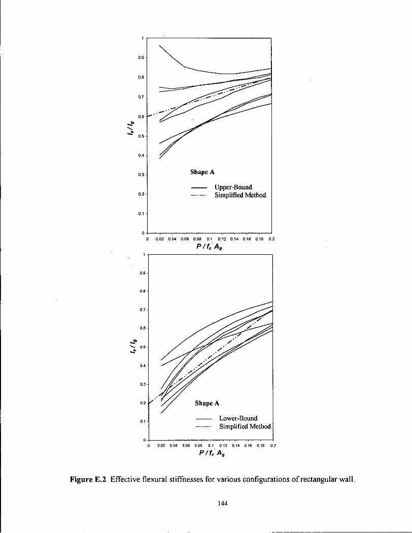
0.8
0.7
0.6
0.4
0.2
Shape A
Upper-Bound Simplified Method
0 0 02 0.04 0.06 0.08 0.1 0.12 0.14 0.16 0.18 0.2
P/f'Ag
Lower-Bound Simplified Method
0 0.02 0.04 0.06 0.08 0.1 0.12 0.14 0.16 0.18 0.2
P/fcAg
Figure E.2 Effective flexural stiffnesses for various configurations of rectangular wall.
144

0.9
0.8
0.7
0.6
0.4
0.3
0.2
Shape B
Upper-Bound Simplified Method
0 0.02 0.04 0.06 0.08 0.1 0.12 0.14 0.16 0.18 0.2
P/fcAg
0.7
0.5
y Shape B
Lower-Bound Simplified Method
0 0.02 0.04 0.06 0.08 0.1 0.12 0.14 0.16 0.18 0.2
P/fcAg
Figure E.3 Effective flexural stiffnesses for various configurations of flanged wall.
145

Figure E.4 Effective flexural stiffnesses for various configurations of C shape wall.
146
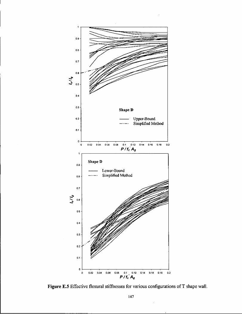
0.9 •
Shape D
0.2 Upper-Bound Simplified Method
0 0 02 0.04 0.06 0.08 0.1 0.12 0.14 0.16 0.18 0.2
P/fC Ag
Shape D
Lower-Bound Simplified Method
0.7
0.6
0.5 •
0.4 •
0.3
0.2-K
0.1
- I r -
0 0.02 0.04 0.06 0.08 0.1 0.12 0.14 0.16 0.18 0.2
P/fcAg
Figure E.5 Effective flexural stiffnesses for various configurations of T shape wall.
147

Appendix F
Computational Procedure for Determining
Effective Member Stiffness
Computational procedure to determine the effective member stiffness, EJe, using the equal
rotation criteria (i.e., equivalent rotation between the two ends of the member).
• Illustrative example:
P
a) Wall element b) B . M . Distribution
M
c) Material modeling d) Curvature distribution
0 = j*0 (x) dx
For similar rotation between the two ends of the member whether computed by actual or
idealized curvature distributions:
JV(x)rfxldealized= jV(x)dx Actual
148

J E j J
EJe = J-M(x)dx Area under B.M.D M(x) Area under actual <f> dlst. EJ(x)CX
i _ YJM(x)Ax
If Ax is constant:
Y ^ L A X ^EJ(x)
_ I > ( x )
^ M{x) [F.l]
^EJ{x)
To implement this procedure in "2Frame-NU\ any wall member is discritized into 99 layers.
98 H 99
MK
a) Wall member b) Discritized B.M.D c) Definition of EJC
2 > , [F.2]
Depending on the moment distribution along the length of the member (single curvature or
double curvature moment diagram), different cases to compute the effective member stiffness are
identified and described:
149
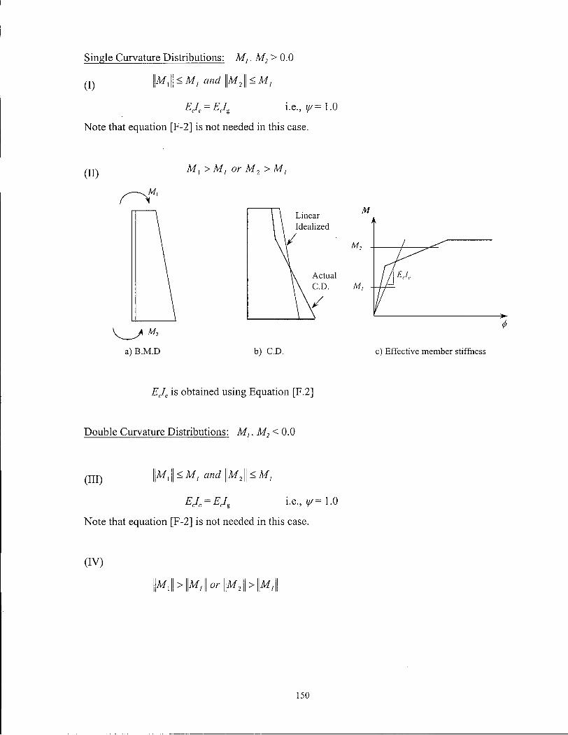
Single Curvature Distributions: M,. M2> 0.0
(I) ll^i I - M, and \\M2|| < M,
EJe = EJ& i.e., ^ = 1 . 0
Note that equation [F-2] is not needed in this case.
a) B . M . D b) C D .
EJe is obtained using Equation [F.2]
Double Curvature Distributions: M,.M2< 0.0
(HI) Ir i II - and \\M2 || < M,
EJ=EJ% i.e., t//=1.0
Note that equation [F-2] is not needed in this case.
(IV)
||Af, || > ||Af, || or i M j I ^ f M ,
150

M
a) B .M.D b) C D . c) Effective member stiffness
In this particular case, point of contraflexure is determined along the length of the member.
Equation [F.2] is applied twice, one for each side resulting in Ejj and EJ/. Note that number of
layers are adjusted according to the length of each side.
Effective member stiffness, EJe, is considered as the equivalent sum of the two springs
(stiffnesses) connected in series. Each stiffness is weighted by its appropriate length of the
member.
EJ. EJ: V E J : v EJ 2 * ( — ) + Ej/ *(—)
L L EJE E I 1*EI 2
c e c e
EI =\i/ E I = c e ' c £?
EJE
]*EJE
2
EJ^i^+EJ2*^)
[F.3]
151

Appendix G
Program "Wall-Tools"
Program "Wall-Tools" is designed for structural engineers performing seismic analysis and
design of reinforced concrete walls. The program provides three basic analysis tools essential in
the flexural design of concrete sections:
1- Moment Curvature Analysis: the bending moment-curvature characteristics of a reinforced
concrete section is determined for given axial load until default, or user defined strain limits
are reached. The analysis is performed for a single axial load level or for a range of axial
loads expected on the described reinforced concrete section. Idealized tri-linear
approximations to the theoretical moment-curvature relation are also calculated. Strain
profile across the section is given at any moment state.
2- Axial Load - Bending Moment Interaction: nominal moment capacity of the reinforced
concrete section is calculated for the entire range of axial load. The capacity is controlled
either by reaching maximum strain limits or by checking the ultimate resistance at a cracked
section location. Factored, Nominal, and Probable resistance factors are allowed.
3- Effective Flexural Stiffness: flexural stiffness of reinforced concrete shear wall is determined
based on the characteristics of the cross section at the base. Trilinear approximation of the
moment curvature relation of the cross section at the base along with the assumption of axial
gravity being linear with height are used to construct the curvature distribution over the wall
height. The force-displacement curve is obtained by integrating the curvature distribution
over the wall height repeatedly for different load steps. The program uses the equal energy
(area) principle of the force-displacement curve to determine the equivalent bilinear
idealization.
Program features include:
• Dual SI and Imperial units.
• User friendly input format.
• Full tabular output and graphical representation.
152

153