Embed Size (px)
Citation preview

This page intentionally left blank
L INEAR ALGEBRAA Geometr ic Approach second edition

This page intentionally left blank
L INEAR ALGEBRAA Geometr ic Approach second edition
Theodore ShifrinMalcolm R.AdamsUniversity of Georgia
W.H. Freeman and CompanyNewYork

Publisher: Ruth BaruthSenior Acquisitions Editor: Terri WardExecutive Marketing Manager: Jennifer SomervilleAssociate Editor: Katrina WilhelmEditorial Assistant: Lauren KimmichPhoto Editor: Bianca MoscatelliCover and Text Designer: Blake LoganProject Editors: Leigh Renhard and Techsetters, Inc.Illustrations: Techsetters, Inc.Senior Illustration Coordinator: Bill PageProduction Manager: Ellen CashComposition: Techsetters, Inc.Printing and Binding: RR Donnelley
Library of Congress Control Number: 2010921838
ISBN-13: 978-1-4292-1521-3ISBN-10: 1-4292-1521-6© 2011, 2002 by W. H. Freeman and CompanyAll rights reserved
Printed in the United States of America
First printing
W. H. Freeman and Company41 Madison AvenueNew York, NY 10010Houndmills, Basingstoke RG21 6XS, Englandwww.whfreeman.com

v
CONTENTS
Preface viiForeword to the Instructor xiiiForeword to the Student xvii
Chapter 1 Vectors and Matrices 11. Vectors 12. Dot Product 183. Hyperplanes in Rn 284. Systems of Linear Equations and Gaussian Elimination 365. The Theory of Linear Systems 536. Some Applications 64
Chapter 2 Matrix Algebra 811. Matrix Operations 812. Linear Transformations: An Introduction 913. Inverse Matrices 1024. Elementary Matrices: Rows Get Equal Time 1105. The Transpose 119
Chapter 3 Vector Spaces 1271. Subspaces of Rn 1272. The Four Fundamental Subspaces 1363. Linear Independence and Basis 1434. Dimension and Its Consequences 1575. A Graphic Example 1706. Abstract Vector Spaces 176
vi Contents
Chapter 4 Projections and Linear Transformations 1911. Inconsistent Systems and Projection 1912. Orthogonal Bases 2003. The Matrix of a Linear Transformation and the
Change-of-Basis Formula 2084. Linear Transformations on Abstract Vector Spaces 224
Chapter 5 Determinants 2391. Properties of Determinants 2392. Cofactors and Cramer’s Rule 2453. Signed Area in R2 and Signed Volume in R3 255
Chapter 6 Eigenvalues and Eigenvectors 2611. The Characteristic Polynomial 2612. Diagonalizability 2703. Applications 2774. The Spectral Theorem 286
Chapter 7 Further Topics 2991. Complex Eigenvalues and Jordan Canonical Form 2992. Computer Graphics and Geometry 3143. Matrix Exponentials and Differential Equations 331
For Further Reading 349Answers to Selected Exercises 351List of Blue Boxes 367Index 369

vii
P REFACE
O ne of the most enticing aspects of mathematics, we have found, is the interplay ofideas from seemingly disparate disciplines of the subject. Linear algebra providesa beautiful illustration of this, in that it is by nature both algebraic and geometric.
Our intuition concerning lines and planes in space acquires an algebraic interpretation thatthen makes sense more generally in higher dimensions. What’s more, in our discussion ofthe vector space concept, we will see that questions from analysis and differential equationscan be approached through linear algebra. Indeed, it is fair to say that linear algebra liesat the foundation of modern mathematics, physics, statistics, and many other disciplines.Linear problems appear in geometry, analysis, and many applied areas. It is this multifacetedaspect of linear algebra that we hope both the instructor and the students will find appealingas they work through this book.
From a pedagogical point of view, linear algebra is an ideal subject for students to learnto think about mathematical concepts and to write rigorous mathematical arguments. Oneof our goals in writing this text—aside from presenting the standard computational aspectsand some interesting applications—is to guide the student in this endeavor. We hope thisbook will be a thought-provoking introduction to the subject and its myriad applications,one that will be interesting to the science or engineering student but will also help themathematics student make the transition to more abstract advanced courses.
We have tried to keep the prerequisites for this book to a minimum. Although manyof our students will have had a course in multivariable calculus, we do not presuppose anyexposure to vectors or vector algebra. We assume only a passing acquaintance with thederivative and integral in Section 6 of Chapter 3 and Section 4 of Chapter 4. Of course,in the discussion of differential equations in Section 3 of Chapter 7, we expect a bit more,including some familiarity with power series, in order for students to understand the matrixexponential.
In the second edition, we have added approximately 20% more examples (a number ofwhich are sample proofs) and exercises—most computational, so that there are now over210 examples and 545 exercises (many with multiple parts). We have also added solutionsto many more exercises at the back of the book, hoping that this will help some of thestudents; in the case of exercises requiring proofs, these will provide additional workedexamples that many students have requested. We continue to believe that good exercisesare ultimately what makes a superior mathematics text.
In brief, here are some of the distinctive features of our approach:
• We introduce geometry from the start, using vector algebra to do a bit of analyticgeometry in the first section and the dot product in the second.
viii Preface
• We emphasize concepts and understanding why, doing proofs in the text and askingthe student to do plenty in the exercises. To help the student adjust to a higher levelof mathematical rigor, throughout the early portion of the text we provide “blueboxes” discussing matters of logic and proof technique or advice on formulatingproblem-solving strategies. A complete list of the blue boxes is included at the endof the book for the instructor’s and the students’ reference.
• We use rotations, reflections, and projections in R2 as a first brush with the notion ofa linear transformation when we introduce matrix multiplication; we then treat lineartransformations generally in concert with the discussion of projections. Thus, wemotivate the change-of-basis formula by starting with a coordinate system in whicha geometrically defined linear transformation is clearly understood and asking forits standard matrix.
• We emphasize orthogonal complements and their role in finding a homogeneoussystem of linear equations that defines a given subspace of Rn.
• In the last chapter we include topics for the advanced student, such as Jordancanonical form, a classification of the motions of R2 and R3, and a discussion ofhow Mathematica draws two-dimensional images of three-dimensional shapes.
The historical notes at the end of each chapter, prepared with the generous assistance ofPaul Lorczak for the first edition, have been left as is. We hope that they give readers anidea how the subject developed and who the key players were.
A few words on miscellaneous symbols that appear in the text: We have marked withan asterisk (∗) the problems for which there are answers or solutions at the back of the text.As a guide for the new teacher, we have also marked with a sharp (�) those “theoretical”exercises that are important and to which reference is made later. We indicate the end of aproof by the symbol .
Significant Changes in the Second Edition• We have added some examples (particularly of proof reasoning) to Chapter 1 and
streamlined the discussion in Sections 4 and 5. In particular, we have included afairly simple proof that the rank of a matrix is well defined and have outlined inan exercise how this simple proof can be extended to show that reduced echelonform is unique. We have also introduced the Leslie matrix and an application topopulation dynamics in Section 6.
• We have reorganized Chapter 2, adding two new sections: one on linear transfor-mations and one on elementary matrices. This makes our introduction of lineartransformations more detailed and more accessible than in the first edition, pavingthe way for continued exploration in Chapter 4.
• We have combined the sections on linear independence and basis and noticeablystreamlined the treatment of the four fundamental subspaces throughout Chapter3. In particular, we now obtain all the orthogonality relations among these foursubspaces in Section 2.
• We have altered Section 1 of Chapter 4 somewhat and have completely reorga-nized the treatment of the change-of-basis theorem. Now we treat first linear mapsT : Rn → Rn in Section 3, and we delay to Section 4 the general case and linearmaps on abstract vector spaces.
• We have completely reorganized Chapter 5, moving the geometric interpretation ofthe determinant from Section 1 to Section 3. Until the end of Section 1, we havetied the computation of determinants to row operations only, proving at the end thatthis implies multilinearity.
Preface ix
• To reiterate, we have added approximately 20% more exercises, most elementaryand computational in nature. We have included more solved problems at the backof the book and, in many cases, have added similar new exercises. We have addedsome additional blue boxes, as well as a table giving the locations of them all.And we have added more examples early in the text, including more sample proofarguments.
Comments on Individual ChaptersWe begin in Chapter 1 with a treatment of vectors, first in R2 and then in higher dimensions,emphasizing the interplay between algebra and geometry. Parametric equations of lines andplanes and the notion of linear combination are introduced in the first section, dot productsin the second. We next treat systems of linear equations, starting with a discussion ofhyperplanes in Rn, then introducing matrices and Gaussian elimination to arrive at reducedechelon form and the parametric representation of the general solution. We then discussconsistency and the relation between solutions of the homogeneous and inhomogeneoussystems. We conclude with a selection of applications.
In Chapter 2 we treat the mechanics of matrix algebra, including a first brush with2 × 2 matrices as geometrically defined linear transformations. Multiplication of matrices isviewed as a generalization of multiplication of matrices by vectors, introduced in Chapter 1,but then we come to understand that it represents composition of linear transformations.We now have separate sections for inverse matrices and elementary matrices (where theLU decomposition is introduced) and introduce the notion of transpose. We expect thatmost instructors will treat elementary matrices lightly.
The heart of the traditional linear algebra course enters in Chapter 3, where we dealwith subspaces, linear independence, bases, and dimension. Orthogonality is a majortheme throughout our discussion, as is the importance of going back and forth betweenthe parametric representation of a subspace of Rn and its definition as the solution setof a homogeneous system of linear equations. In the fourth section, we officially give thealgorithms for constructing bases for the four fundamental subspaces associated to a matrix.In the optional fifth section, we give the interpretation of these fundamental subspaces inthe context of graph theory. In the sixth and last section, we discuss various examples of“abstract” vector spaces, concentrating on matrices, polynomials, and function spaces. TheLagrange interpolation formula is derived by defining an appropriate inner product on thevector space of polynomials.
In Chapter 4 we continue with the geometric flavor of the course by discussing pro-jections, least squares solutions of inconsistent systems, and orthogonal bases and theGram-Schmidt process. We continue our study of linear transformations in the context ofthe change-of-basis formula. Here we adopt the viewpoint that the matrix of a geometricallydefined transformation is often easy to calculate in a coordinate system adapted to the ge-ometry of the situation; then we can calculate its standard matrix by changing coordinates.The diagonalization problem emerges as natural, and we will return to it fully in Chapter 6.
We give a more thorough treatment of determinants in Chapter 5 than is typical forintroductory texts. We have, however, moved the geometric interpretation of signed areaand signed volume to the last section of the chapter. We characterize the determinant byits behavior under row operations and then give the usual multilinearity properties. In thesecond section we give the formula for expanding a determinant in cofactors and concludewith Cramer’s Rule.
Chapter 6 is devoted to a thorough treatment of eigenvalues, eigenvectors, diago-nalizability, and various applications. In the first section we introduce the characteristicpolynomial, and in the second we introduce the notions of algebraic and geometric multi-plicity and give a sufficient criterion for a matrix with real eigenvalues to be diagonalizable.
x Preface
In the third section, we solve some difference equations, emphasizing how eigenvalues andeigenvectors give a “normal mode” decomposition of the solution. We conclude the sec-tion with an optional discussion of Markov processes and stochastic matrices. In the lastsection, we prove the Spectral Theorem, which we believe to be—at least in this most basicsetting—one of the important theorems all mathematics majors should know; we include abrief discussion of its application to conics and quadric surfaces.
Chapter 7 consists of three independent special topics. In the first section, we discussthe two obstructions that have arisen in Chapter 6 to diagonalizing a matrix—complexeigenvalues and repeated eigenvalues. Although Jordan canonical form does not ordinarilyappear in introductory texts, it is conceptually important and widely used in the studyof systems of differential equations and dynamical systems. In the second section, wegive a brief introduction to the subject of affine transformations and projective geometry,including discussions of the isometries (motions) of R2 and R3. We discuss the notionof perspective projection, which is how computer graphics programs draw images on thescreen. An amusing theoretical consequence of this discussion is the fact that circles,ellipses, parabolas, and hyperbolas are all “projectively equivalent” (i.e., can all be seen byprojecting any one on different viewing screens). The third, and last, section is perhaps themost standard, presenting the matrix exponential and applications to systems of constant-coefficient ordinary differential equations. Once again, eigenvalues and eigenvectors playa central role in “uncoupling” the system and giving rise, physically, to normal modes.
AcknowledgmentsWe would like to thank our many colleagues and students who’ve suggested improvementsto the text. We give special thanks to our colleagues Ed Azoff and Roy Smith, who havesuggested improvements for the second edition. Of course, we thank all our students whohave endured earlier versions of the text and made suggestions to improve it; we wouldlike to single out Victoria Akin, Paul Iezzi, Alex Russov, and Catherine Taylor for specificcontributions. We appreciate the enthusiastic and helpful support of Terri Ward and KatrinaWilhelm at W. H. Freeman. We would also like to thank the following colleagues aroundthe country, who reviewed the manuscript and offered many helpful comments for theimproved second edition:
Richard Blecksmith Northern Illinois UniversityMike Daven Mount Saint Mary CollegeJochen Denzler The University of TennesseeDarren Glass Gettsyburg CollegeS. P. Hastings University of PittsburghXiang-dong Hou University of South FloridaShafiu Jibrin Northern Arizona UniversityKimball Martin The University of OklahomaManouchehr Misaghian Johnson C. Smith UniversityS. S. Ravindran The University of Alabama in HuntsvilleWilliam T. Ross University of RichmondDan Rutherford Duke UniversityJames Solazzo Coastal Carolina UniversityJeffrey Stuart Pacific Lutheran UniversityAndrius Tamulis Cardinal Stritch University
In addition, the authors thank Paul Lorczak and Brian Bradie for their contributions to thefirst edition of the text. We are also indebted to Gil Strang for shaping the way most of ushave taught linear algebra during the last decade or two.

Preface xi
The authors welcome your comments and suggestions. Please address any e-mailcorrespondence to [email protected] or [email protected] . Andplease keep an eye on
http://www.math.uga.edu/˜shifrin/LinAlgErrata.pdf
for information on any typos and corrections.

This page intentionally left blank

xiii
FOREWORD TO THE INSTRUCTOR
W e have provided more material than most (dare we say all?) instructors cancomfortably cover in a one-semester course. We believe it is essential to plan thecourse so as to have time to come to grips with diagonalization and applications
of eigenvalues, including at least one day devoted to the Spectral Theorem. Thus, everyinstructor will have to make choices and elect to treat certain topics lightly, and others notat all. At the end of this Foreword we present a time frame that we tend to follow, but ina standard-length semester with only three hours a week, one must obviously make somechoices and some sacrifices. We cannot overemphasize the caveat that one must be carefulto move through Chapter 1 in a timely fashion: Even though it is tempting to plumb thedepths of every idea in Chapter 1, we believe that spending one-third of the course onChapters 1 and 2 is sufficient. Don’t worry: As you progress, you will revisit and reinforcethe basic concepts in the later chapters.
It is also possible to use this text as a second course in linear algebra for studentswho’ve had a computational matrix algebra course. For such a course, there should beample material to cover, treading lightly on the mechanics and spending more time on thetheory and various applications, especially Chapter 7.
If you’re using this book as your text, we assume that you have a predisposition toteaching proofs and an interest in the geometric emphasis we have tried to provide. Webelieve strongly that presenting proofs in class is only one ingredient; the students mustplay an active role by wrestling with proofs in homework as well. To this end, we haveprovided numerous exercises of varying levels of difficulty that require the students towrite proofs. Generally speaking, exercises are arranged in order of increasing difficulty,starting with the computational and ending with the more challenging. To offer a bit moreguidance, we have marked with an asterisk (*) those problems for which answers, hints, ordetailed proofs are given at the back of the book, and we have marked with a sharp (�) themore theoretical problems that are particularly important (and to which reference is madelater). We have added a good number of “asterisked” problems in the second edition. AnInstructor’s Solutions Manual is available from the publisher.
Although we have parted ways with most modern-day authors of linear algebra text-books by avoiding technology, we have included a few problems for which a good calculatoror computer software will be more than helpful. In addition, when teaching the course, weencourage our students to take advantage of their calculators or available software (e.g.,Maple, Mathematica, or MATLAB) to do routine calculations (e.g., reduction to reducedechelon form) once they have mastered the mechanics. Those instructors who are strongbelievers in the use of technology will no doubt have a preferred supplementary manual touse.
xiv Foreword to the Instructor
We would like to comment on a few issues that arise when we teach this course.
1. Distinguishing among points in Rn, vectors starting at the origin, and vectorsstarting elsewhere is always a confusing point at the beginning of any introductorylinear algebra text. The rigorous way to deal with this is to define vectors asequivalence classes of ordered pairs of points, but we believe that such an abstractdiscussion at the outset would be disastrous. Instead, we choose to define vectorsto be the “bound” vectors, i.e., the points in the vector space. On the other hand,we use the notion of “free” vector intuitively when discussing geometric notionsof vector addition, lines, planes, and the like, because we feel it is essential forour students to develop the geometric intuition that is ubiquitous in physics andgeometry.
2. Another mathematical and pedagogical issue is that of using only column vec-tors to represent elements of Rn. We have chosen to start with the notation
x = (x1, . . . , xn) and switch to the column vector
⎡⎢⎢⎣x1
...
xn
⎤⎥⎥⎦ when we introduce ma-
trices in Section 1.4. But for reasons having to do merely with typographical ease,we have not hesitated to use the previous notation from time to time in the text orin exercises when it should cause no confusion.
3. We would encourage instructors using our book for the first time to treat certaintopics gently: The material of Section 2.3 is used most prominently in the treatmentof determinants. We generally find that it is best to skip the proof of the fundamentalTheorem 4.5 in Chapter 3, because we believe that demonstrating it carefully inthe case of a well-chosen example is more beneficial to the students. Similarly, wetread lightly in Chapter 5, skipping the proof of Proposition 2.2 in an introductorycourse. Indeed, when we’re pressed for time, we merely remind students of thecofactor expansion in the 3 × 3 case, prove Cramer’s Rule, and move on to Chapter6. We have moved the discussion of the geometry of determinants to Section 3;instructors who have the extra day or so should certainly include it.
4. To us, one of the big stories in this course is going back and forth between the twoways of describing a subspace V ⊂ Rn:
implicit descriptionAx = 0
Gaussianelimination �
�constraintequations
parametric description
x = t1v1 + · · · + tkvk
Gaussian elimination gives a basis for the solution space. On the other hand,finding constraint equations that b must satisfy in order to be a linear combination ofv1, . . . , vk gives a system of equations whose solutions are precisely the subspacespanned by v1, . . . , vk .
5. Because we try to emphasize geometry and orthogonality more than most texts,we introduce the orthogonal complement of a subspace early in Chapter 3. Inrewriting, we have devoted all of Section 2 to the four fundamental subspaces.We continue to emphasize the significance of the equalities N(A) = R(A)⊥ andN(AT) = C(A)⊥ and the interpretation of the latter in terms of constraint equations.Moreover, we have taken advantage of this interpretation to deduce the companionequalities C(A) = N(AT)⊥ and R(A) = N(A)⊥ immediately, rather than delaying
Foreword to the Instructor xv
these as in the first edition. It was confusing enough for the instructor—let alonethe poor students—to try to keep track of which we knew and which we didn’t. (Todeduce (V ⊥)⊥ = V for the general subspace V ⊂ Rn, we need either dimensionor the (more basic) fact that every such V has a basis and hence can be expressedas a row or column space.) We hope that our new treatment is both more efficientand less stressful for the students.
6. We always end the course with a proof of the Spectral Theorem and a few daysof applications, usually including difference equations and Markov processes (butskipping the optional Section 6.3.1), conics and quadrics, and, if we’re lucky, afew days on either differential equations or computer graphics. We do not coverSection 7.1 at all in an introductory course.
7. Instructors who choose to cover abstract vector spaces (Section 3.6) and lineartransformations on them (Section 4.4) will discover that most students find thismaterial quite challenging. Afew of the exercises will require some calculus skills.
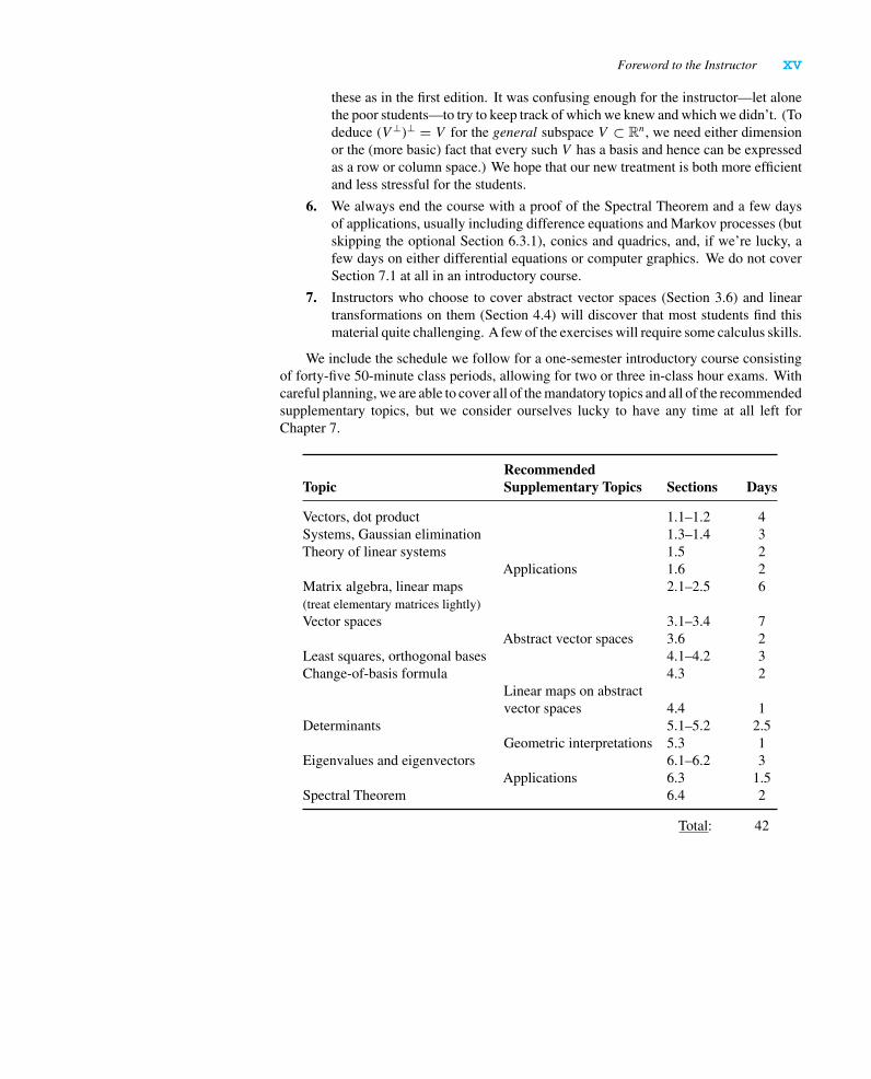
We include the schedule we follow for a one-semester introductory course consistingof forty-five 50-minute class periods, allowing for two or three in-class hour exams. Withcareful planning, we are able to cover all of the mandatory topics and all of the recommendedsupplementary topics, but we consider ourselves lucky to have any time at all left forChapter 7.
TopicRecommendedSupplementary Topics Sections Days
Vectors, dot product 1.1–1.2 4Systems, Gaussian elimination 1.3–1.4 3Theory of linear systems 1.5 2
Applications 1.6 2Matrix algebra, linear maps 2.1–2.5 6(treat elementary matrices lightly)Vector spaces 3.1–3.4 7
Abstract vector spaces 3.6 2Least squares, orthogonal bases 4.1–4.2 3Change-of-basis formula 4.3 2
Linear maps on abstractvector spaces 4.4 1
Determinants 5.1–5.2 2.5Geometric interpretations 5.3 1
Eigenvalues and eigenvectors 6.1–6.2 3Applications 6.3 1.5
Spectral Theorem 6.4 2
Total: 42

This page intentionally left blank

xvii
FOREWORD TO THE STUDENT
W e have tried to write a book that you can read—not like a novel, but with pencilin hand. We hope that you will find it interesting, challenging, and rewardingto learn linear algebra. Moreover, by the time you have completed this course,
you should find yourself thinking more clearly, analyzing problems with greater maturity,and writing more cogent arguments—both mathematical and otherwise. Above all else, wesincerely hope you will have fun.
To learn mathematics effectively, you must read as an active participant, workingthrough the examples in the text for yourself, learning all the definitions, and then attackinglots of exercises—both concrete and theoretical. To this end, there are approximately 550exercises, a large portion of them having multiple parts. These include computations,applied problems, and problems that ask you to come up with examples. There are proofsvarying from the routine to open-ended problems (“Prove or give a counterexample …”)to some fairly challenging conceptual posers. It is our intent to help you in your quest tobecome a better mathematics student. In some cases, studying the examples will providea direct line of approach to a problem, or perhaps a clue. But in others, you will needto do some independent thinking. Many of the exercises ask you to “prove” or “show”something. To help you learn to think through mathematical problems and write proofs,we’ve provided 29 “blue boxes” to help you learn basics about the language of mathematics,points of logic, and some pointers on how to approach problem solving and proof writing.
We have provided many examples that demonstrate the ideas and computational toolsnecessary to do most of the exercises. Nevertheless, you may sometimes believe you haveno idea how to get started on a particular problem. Make sure you start by learning therelevant definitions. Most of the time in linear algebra, if you know the definition, writedown clearly what you are given, and note what it is you are to show, you are more thanhalfway there. In a computational problem, before you mechanically write down a matrixand start reducing it to echelon form, be sure you know what it is about that matrix thatyou are trying to find: its row space, its nullspace, its column space, its left nullspace, itseigenvalues, and so on. In more conceptual problems, it may help to make up an exampleillustrating what you are trying to show; you might try to understand the problem in two orthree dimensions—often a picture will give you insight. In other words, learn to play a bitwith the problem and feel more comfortable with it. But mathematics can be hard work,and sometimes you should leave a tough problem to “brew” in your brain while you go onto another problem—or perhaps a good night’s sleep—to return to it tomorrow.
Remember that in multi-part problems, the hypotheses given at the outset hold through-out the problem. Moreover, usually (but not always) we have arranged such problems insuch a way that you should use the results of part a in trying to do part b, and so on. For theproblems marked with an asterisk (∗) we have provided either numerical answers or, in the

xviii Foreword to the Student
case of proof exercises, solutions (some more detailed than others) at the back of the book.Resist as long as possible the temptation to refer to the solutions! Try to be sure you’veworked the problem correctly before you glance at the answer. Be careful: Some solutionsin the book are not complete, so it is your responsiblity to fill in the details. The problemsthat are marked with a sharp (�) are not necessarily particularly difficult, but they generallyinvolve concepts and results to which we shall refer later in the text. Thus, if your instructorassigns them, you should make sure you understand how to do them. Occasional exercisesare quite challenging, and we hope you will work hard on a few; we firmly believe that onlyby struggling with a real puzzler do we all progress as mathematicians.
Once again, we hope you will have fun as you embark on your voyage to learn linearalgebra. Please let us know if there are parts of the book you find particularly enjoyable ortroublesome.
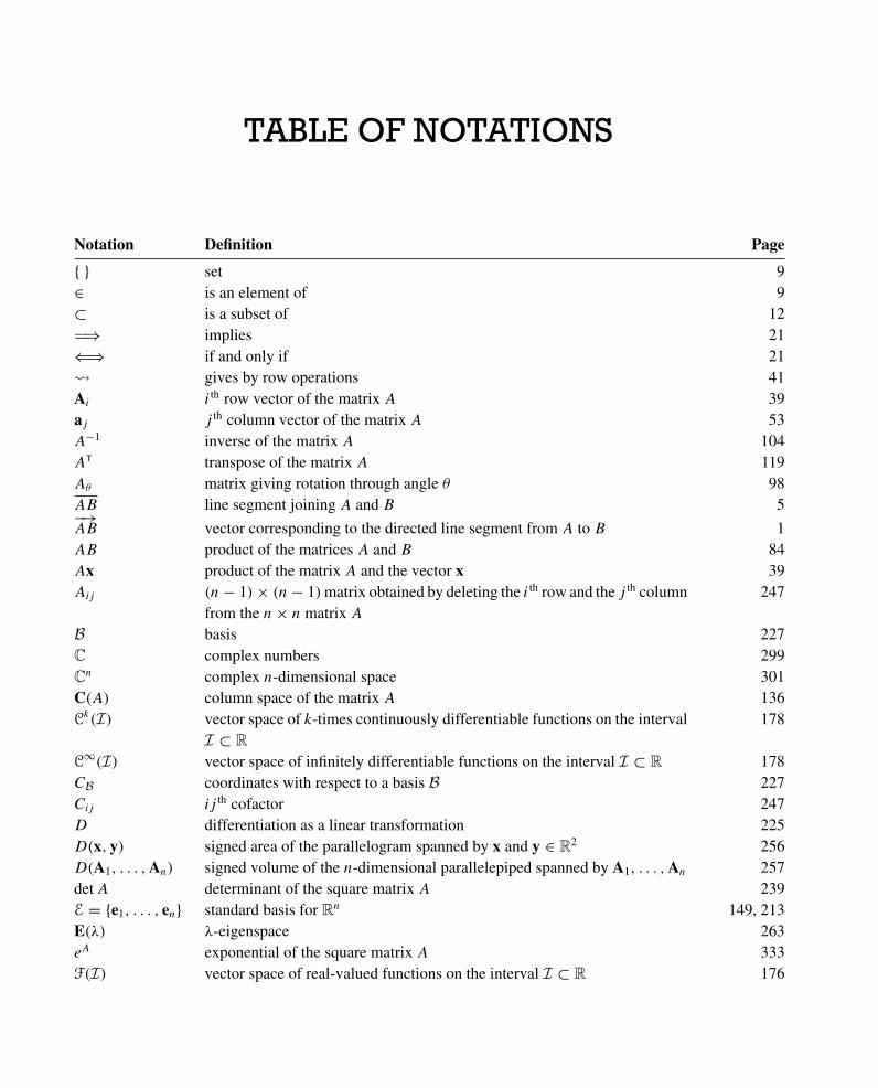
TABLE OF NOTATIONS
Notation Definition Page
{ } set 9∈ is an element of 9⊂ is a subset of 12�⇒ implies 21⇐⇒ if and only if 21� gives by row operations 41Ai i th row vector of the matrix A 39aj j th column vector of the matrix A 53A−1 inverse of the matrix A 104AT transpose of the matrix A 119Aθ matrix giving rotation through angle θ 98AB line segment joining A and B 5−→AB vector corresponding to the directed line segment from A to B 1AB product of the matrices A and B 84Ax product of the matrix A and the vector x 39Aij (n− 1)× (n− 1)matrix obtained by deleting the i th row and the j th column
from the n× n matrix A247
B basis 227C complex numbers 299Cn complex n-dimensional space 301C(A) column space of the matrix A 136Ck(I) vector space of k-times continuously differentiable functions on the interval
I ⊂ R
178
C∞(I) vector space of infinitely differentiable functions on the interval I ⊂ R 178CB coordinates with respect to a basis B 227Cij ij th cofactor 247D differentiation as a linear transformation 225D(x, y) signed area of the parallelogram spanned by x and y ∈ R2 256D(A1, . . . ,An) signed volume of the n-dimensional parallelepiped spanned by A1, . . . ,An 257detA determinant of the square matrix A 239E = {e1, . . . , en} standard basis for Rn 149, 213E(λ) λ-eigenspace 263eA exponential of the square matrix A 333F(I) vector space of real-valued functions on the interval I ⊂ R 176
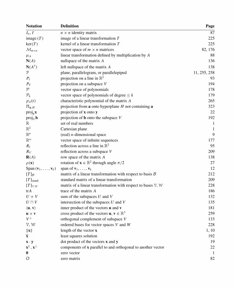
Notation Definition Page
In, I n× n identity matrix 87image (T ) image of a linear transformation T 225ker(T ) kernel of a linear transformation T 225Mm×n vector space of m× n matrices 82, 176μA linear transformation defined by multiplication by A 88N(A) nullspace of the matrix A 136
N(AT) left nullspace of the matrix A 138P plane, parallelogram, or parallelepiped 11, 255, 258P� projection on a line in R2 93PV projection on a subspace V 194P vector space of polynomials 178Pk vector space of polynomials of degree ≤ k 179pA(t) characteristic polynomial of the matrix A 265�a,H projection from a onto hyperplane H not containing a 323projyx projection of x onto y 22projV b projection of b onto the subspace V 192R set of real numbers 1R2 Cartesian plane 1Rn (real) n-dimensional space 9Rω vector space of infinite sequences 177R� reflection across a line in R2 95RV reflection across a subspace V 209R(A) row space of the matrix A 138ρ(x) rotation of x ∈ R2 through angle π/2 27Span (v1, . . . , vk) span of v1, . . . , vk 12[T ]B matrix of a linear transformation with respect to basis B 212[T ]stand standard matrix of a linear transformation 209[T ]V,W matrix of a linear transformation with respect to bases V, W 228trA trace of the matrix A 186U + V sum of the subspaces U and V 132U ∩ V intersection of the subspaces U and V 135〈u, v〉 inner product of the vectors u and v 181u × v cross product of the vectors u, v ∈ R3 259V ⊥ orthogonal complement of subspace V 133V, W ordered bases for vector spaces V andW 228‖x‖ length of the vector x 1, 10x least squares solution 192x · y dot product of the vectors x and y 19x‖ , x⊥ components of x parallel to and orthogonal to another vector 220 zero vector 1O zero matrix 82
1
C H A P T E R 1VECTORS AND MATRICES
L inear algebra provides a beautiful example of the interplay between two branches ofmathematics: geometry and algebra. We begin this chapter with the geometric concepts
and algebraic representations of points, lines, and planes in the more familiar setting of twoand three dimensions (R2 and R3, respectively) and then generalize to the “n-dimensional”space Rn. We come across two ways of describing (hyper)planes—either parametrically oras solutions of a Cartesian equation. Going back and forth between these two formulationswill be a major theme of this text. The fundamental tool that is used in bridging thesedescriptions is Gaussian elimination, a standard algorithm used to solve systems of linearequations. As we shall see, it also has significant consequences in the theory of systemsof equations. We close the chapter with a variety of applications, some not of a geometricnature.
1 Vectors1.1 Vectors in R2
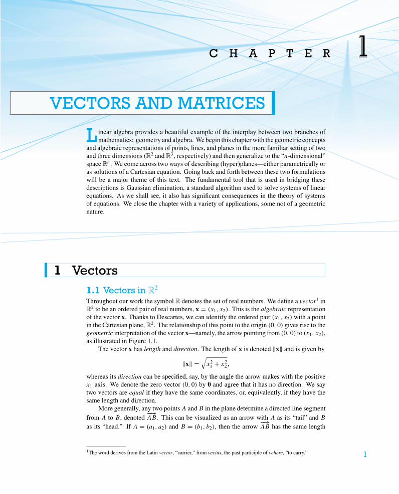
Throughout our work the symbol R denotes the set of real numbers. We define a vector1 inR2 to be an ordered pair of real numbers, x = (x1, x2). This is the algebraic representationof the vector x. Thanks to Descartes, we can identify the ordered pair (x1, x2) with a pointin the Cartesian plane, R2. The relationship of this point to the origin (0, 0) gives rise to thegeometric interpretation of the vector x—namely, the arrow pointing from (0, 0) to (x1, x2),as illustrated in Figure 1.1.
The vector x has length and direction. The length of x is denoted ‖x‖ and is given by
‖x‖ =√x2
1 + x22 ,
whereas its direction can be specified, say, by the angle the arrow makes with the positivex1-axis. We denote the zero vector (0, 0) by 0 and agree that it has no direction. We saytwo vectors are equal if they have the same coordinates, or, equivalently, if they have thesame length and direction.
More generally, any two pointsA and B in the plane determine a directed line segmentfrom A to B, denoted
−→AB. This can be visualized as an arrow with A as its “tail” and B
as its “head.” If A = (a1, a2) and B = (b1, b2), then the arrow−→AB has the same length
1The word derives from the Latin vector, “carrier,” from vectus, the past participle of vehere, “to carry.”
2 Chapter 1 Vectors and Matrices
x = (x1, x2)
O x1
x2
FIGURE 1.1
A
B
C
D
v
O
(b1, b2)
(a1, a2) b1 – a1
b2 – a2
FIGURE 1.2
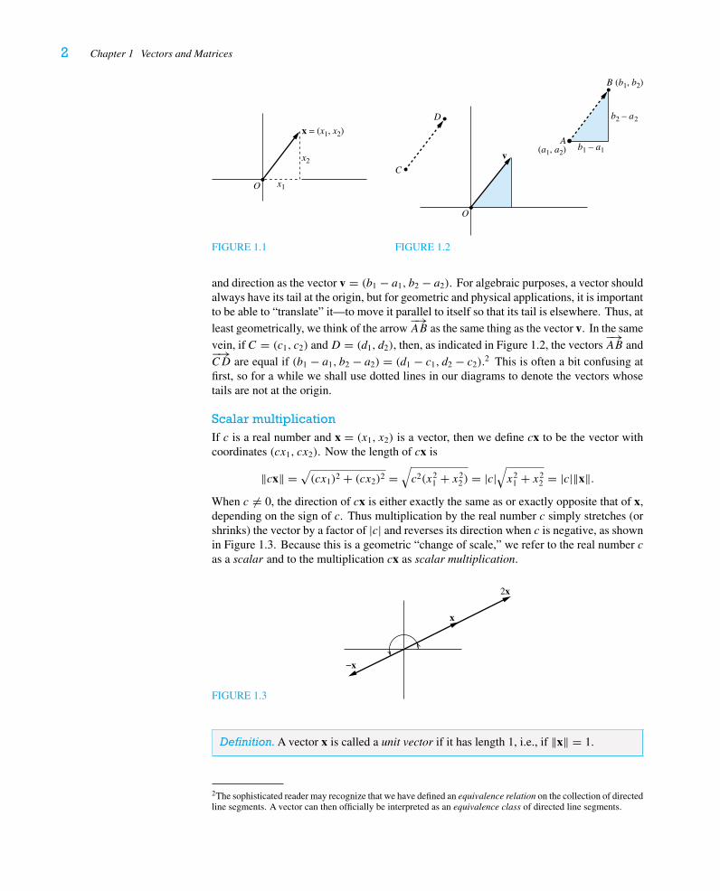
and direction as the vector v = (b1 − a1, b2 − a2). For algebraic purposes, a vector shouldalways have its tail at the origin, but for geometric and physical applications, it is importantto be able to “translate” it—to move it parallel to itself so that its tail is elsewhere. Thus, atleast geometrically, we think of the arrow
−→AB as the same thing as the vector v. In the same
vein, if C = (c1, c2) andD = (d1, d2), then, as indicated in Figure 1.2, the vectors−→AB and−→
CD are equal if (b1 − a1, b2 − a2) = (d1 − c1, d2 − c2).2 This is often a bit confusing atfirst, so for a while we shall use dotted lines in our diagrams to denote the vectors whosetails are not at the origin.
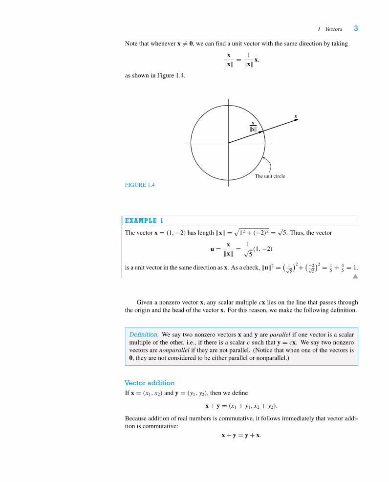
Scalar multiplicationIf c is a real number and x = (x1, x2) is a vector, then we define cx to be the vector withcoordinates (cx1, cx2). Now the length of cx is
‖cx‖ =√(cx1)2 + (cx2)2 =
√c2(x2
1 + x22) = |c|
√x2
1 + x22 = |c|‖x‖.
When c �= 0, the direction of cx is either exactly the same as or exactly opposite that of x,depending on the sign of c. Thus multiplication by the real number c simply stretches (orshrinks) the vector by a factor of |c| and reverses its direction when c is negative, as shownin Figure 1.3. Because this is a geometric “change of scale,” we refer to the real number cas a scalar and to the multiplication cx as scalar multiplication.
FIGURE 1.3
x
−x
2x
Definition.A vector x is called a unit vector if it has length 1, i.e., if ‖x‖ = 1.
2The sophisticated reader may recognize that we have defined an equivalence relation on the collection of directedline segments. A vector can then officially be interpreted as an equivalence class of directed line segments.
1 Vectors 3
Note that whenever x �= 0, we can find a unit vector with the same direction by taking
x‖x‖ = 1
‖x‖x,
as shown in Figure 1.4.
FIGURE 1.4
x
||x||x
The unit circle
EXAMPLE 1
The vector x = (1,−2) has length ‖x‖ = √12 + (−2)2 = √5. Thus, the vector
u = x‖x‖ = 1√
5(1,−2)
is a unit vector in the same direction as x. As a check, ‖u‖2 = ( 1√5
)2+ (−2√5
)2 = 15 + 4
5 = 1.
Given a nonzero vector x, any scalar multiple cx lies on the line that passes throughthe origin and the head of the vector x. For this reason, we make the following definition.
Definition. We say two nonzero vectors x and y are parallel if one vector is a scalarmultiple of the other, i.e., if there is a scalar c such that y = cx. We say two nonzerovectors are nonparallel if they are not parallel. (Notice that when one of the vectors is0, they are not considered to be either parallel or nonparallel.)
Vector additionIf x = (x1, x2) and y = (y1, y2), then we define
x + y = (x1 + y1, x2 + y2).
Because addition of real numbers is commutative, it follows immediately that vector addi-tion is commutative:
x + y = y + x.
4 Chapter 1 Vectors and Matrices
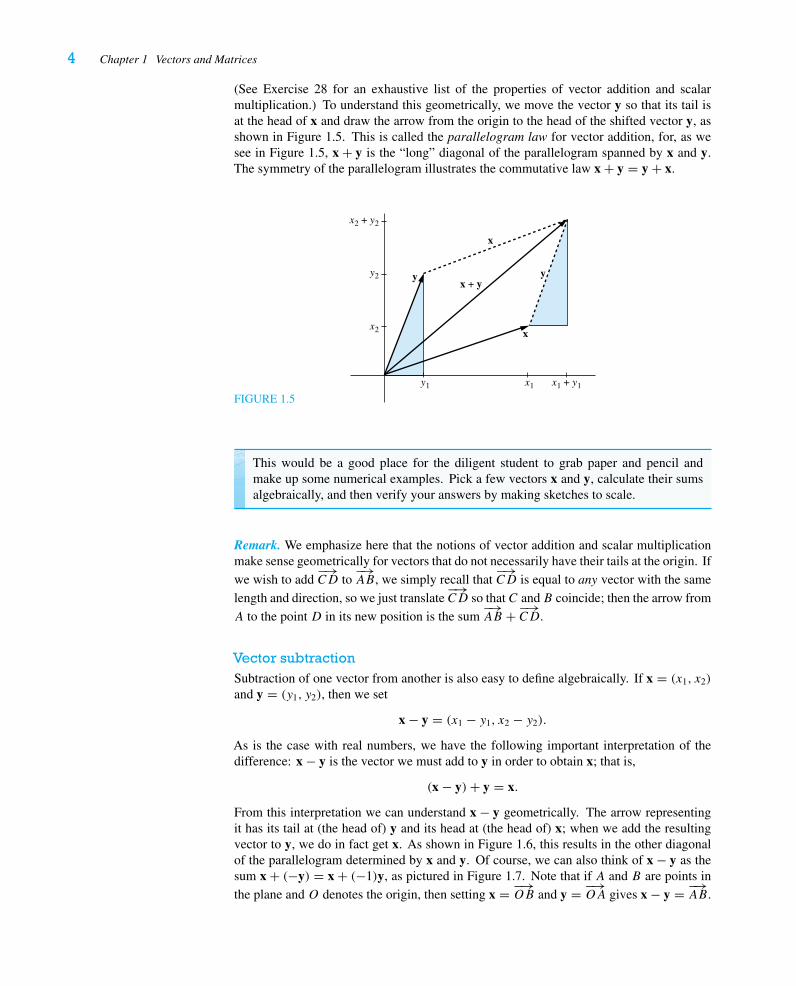
(See Exercise 28 for an exhaustive list of the properties of vector addition and scalarmultiplication.) To understand this geometrically, we move the vector y so that its tail isat the head of x and draw the arrow from the origin to the head of the shifted vector y, asshown in Figure 1.5. This is called the parallelogram law for vector addition, for, as wesee in Figure 1.5, x + y is the “long” diagonal of the parallelogram spanned by x and y.The symmetry of the parallelogram illustrates the commutative law x + y = y + x.
FIGURE 1.5
x
x
y yx + y
x1y1
x2
y2
x1 + y1
x2 + y2
This would be a good place for the diligent student to grab paper and pencil andmake up some numerical examples. Pick a few vectors x and y, calculate their sumsalgebraically, and then verify your answers by making sketches to scale.
Remark. We emphasize here that the notions of vector addition and scalar multiplicationmake sense geometrically for vectors that do not necessarily have their tails at the origin. Ifwe wish to add
−→CD to
−→AB, we simply recall that
−→CD is equal to any vector with the same
length and direction, so we just translate−→CD so that C and B coincide; then the arrow from
A to the point D in its new position is the sum−→AB + −→
CD.
Vector subtractionSubtraction of one vector from another is also easy to define algebraically. If x = (x1, x2)
and y = (y1, y2), then we set
x − y = (x1 − y1, x2 − y2).
As is the case with real numbers, we have the following important interpretation of thedifference: x − y is the vector we must add to y in order to obtain x; that is,
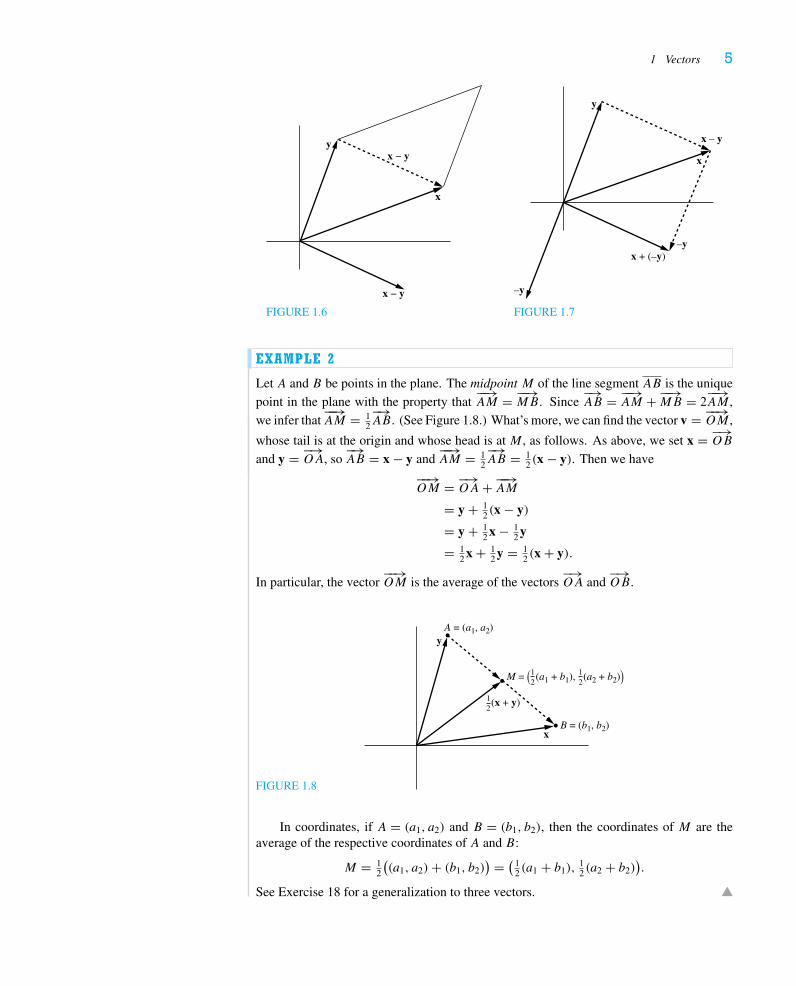
(x − y)+ y = x.
From this interpretation we can understand x − y geometrically. The arrow representingit has its tail at (the head of) y and its head at (the head of) x; when we add the resultingvector to y, we do in fact get x. As shown in Figure 1.6, this results in the other diagonalof the parallelogram determined by x and y. Of course, we can also think of x − y as thesum x + (−y) = x + (−1)y, as pictured in Figure 1.7. Note that if A and B are points inthe plane and O denotes the origin, then setting x = −→
OB and y = −→OA gives x − y = −→
AB.
1 Vectors 5
x
yx − y
x − y
FIGURE 1.6
x
y
x – y
x + (–y)
–y
–y
FIGURE 1.7
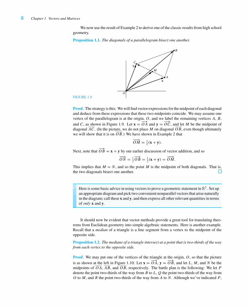
EXAMPLE 2
Let A and B be points in the plane. The midpoint M of the line segment AB is the uniquepoint in the plane with the property that
−−→AM = −−→
MB. Since−→AB = −−→
AM + −−→MB = 2
−−→AM ,
we infer that−−→AM = 1
2
−→AB. (See Figure 1.8.) What’s more, we can find the vector v = −−→
OM ,
whose tail is at the origin and whose head is at M , as follows. As above, we set x = −→OB
and y = −→OA, so
−→AB = x − y and
−−→AM = 1
2
−→AB = 1
2 (x − y). Then we have
−−→OM = −→
OA+ −−→AM
= y + 12 (x − y)
= y + 12 x − 1
2 y
= 12 x + 1
2 y = 12 (x + y).
In particular, the vector−−→OM is the average of the vectors
−→OA and
−→OB.
FIGURE 1.8
A = (a1, a2)
B = (b1, b2)
y
x
12
12
12
(x + y)
M = ( (a1 + b1), (a2 + b2))
In coordinates, if A = (a1, a2) and B = (b1, b2), then the coordinates of M are theaverage of the respective coordinates of A and B:
M = 12
((a1, a2)+ (b1, b2)
) = ( 12 (a1 + b1),
12 (a2 + b2)
).
See Exercise 18 for a generalization to three vectors.
6 Chapter 1 Vectors and Matrices
We now use the result of Example 2 to derive one of the classic results from high schoolgeometry.
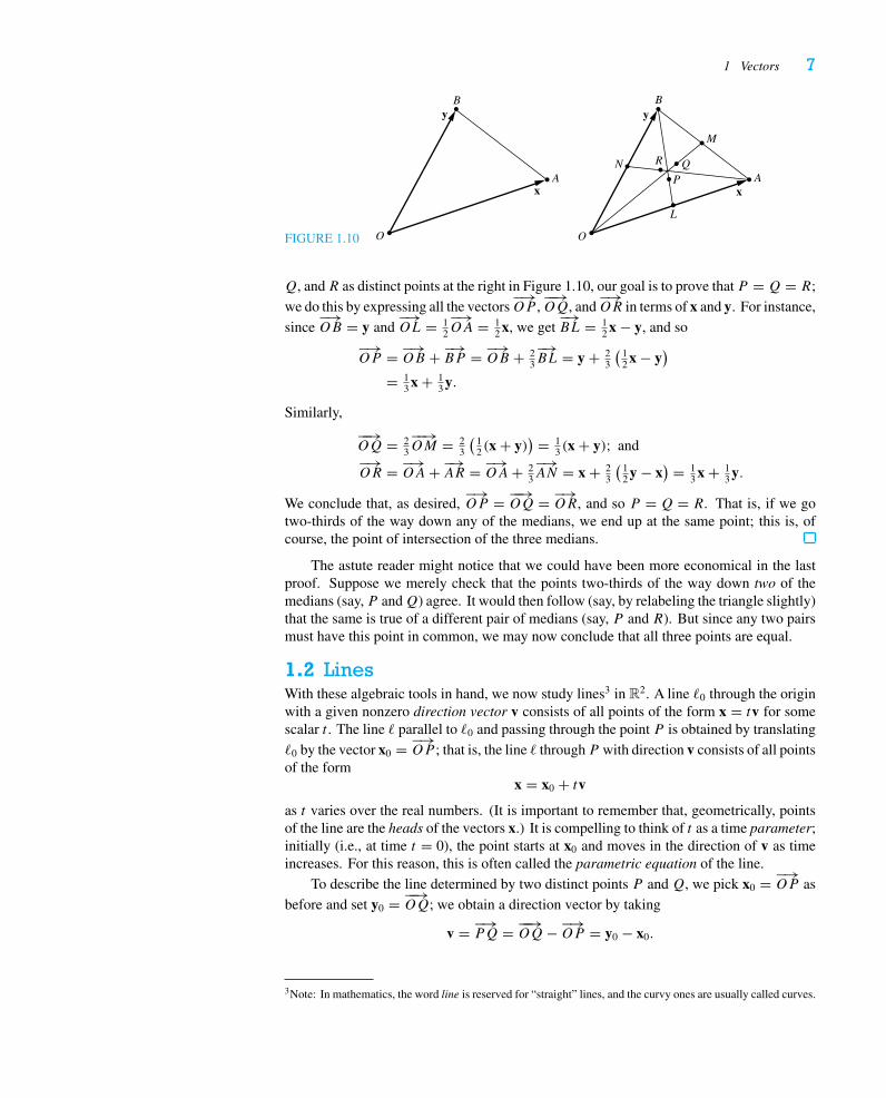
Proposition 1.1. The diagonals of a parallelogram bisect one another.
FIGURE 1.9O
A
B
C
x
yM
Proof. The strategy is this: We will find vector expressions for the midpoint of each diagonaland deduce from these expressions that these two midpoints coincide. We may assume onevertex of the parallelogram is at the origin, O, and we label the remaining vertices A, B,and C, as shown in Figure 1.9. Let x = −→
OA and y = −→OC, and let M be the midpoint of
diagonal AC. (In the picture, we do not placeM on diagonal OB, even though ultimatelywe will show that it is on OB.) We have shown in Example 2 that
−−→OM = 1
2 (x + y).
Next, note that−→OB = x + y by our earlier discussion of vector addition, and so
−−→ON = 1
2
−→OB = 1
2 (x + y) = −−→OM.
This implies that M = N , and so the point M is the midpoint of both diagonals. That is,the two diagonals bisect one another.
Here is some basic advice in using vectors to prove a geometric statement in R2. Set upan appropriate diagram and pick two convenient nonparallel vectors that arise naturallyin the diagram; call these x and y, and then express all other relevant quantities in termsof only x and y.
It should now be evident that vector methods provide a great tool for translating theo-rems from Euclidean geometry into simple algebraic statements. Here is another example.Recall that a median of a triangle is a line segment from a vertex to the midpoint of theopposite side.
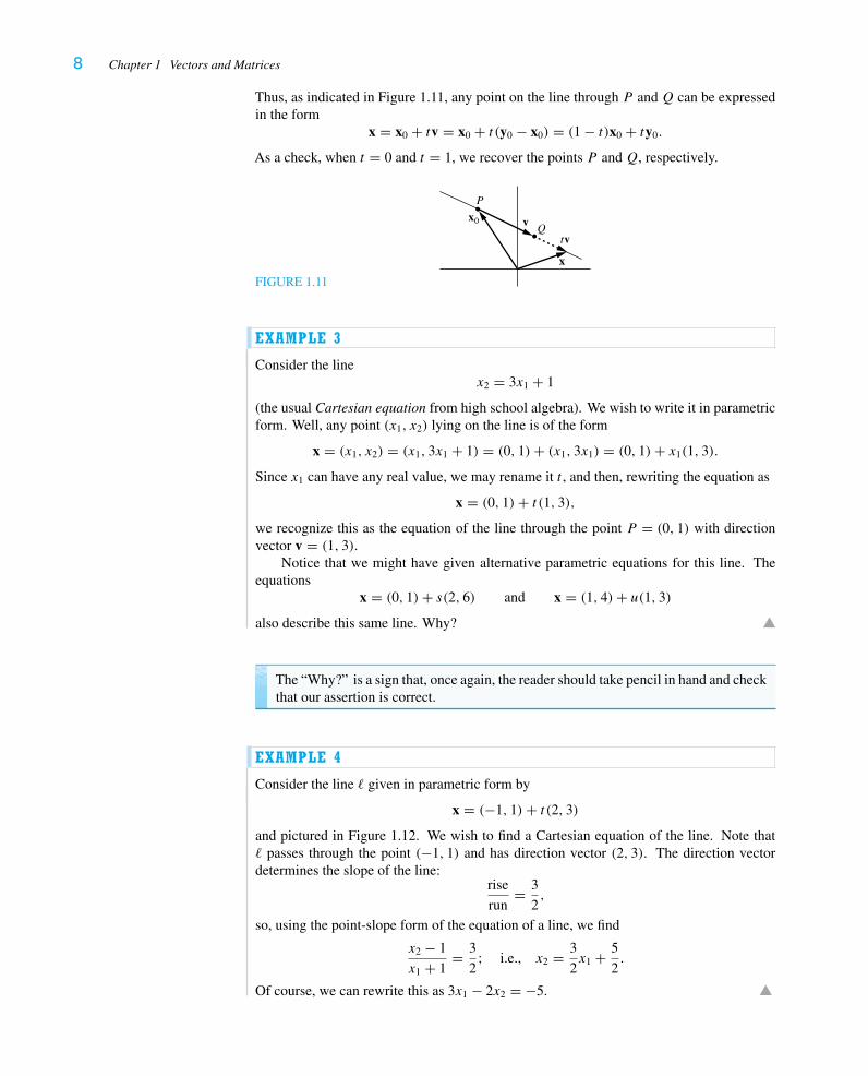
Proposition 1.2. The medians of a triangle intersect at a point that is two-thirds of the wayfrom each vertex to the opposite side.
Proof. We may put one of the vertices of the triangle at the origin, O, so that the pictureis as shown at the left in Figure 1.10: Let x = −→
OA, y = −→OB, and let L, M , and N be the
midpoints of OA, AB, and OB, respectively. The battle plan is the following: We let Pdenote the point two-thirds of the way from B to L,Q the point two-thirds of the way fromO toM , and R the point two-thirds of the way from A to N . Although we’ve indicated P ,
1 Vectors 7
FIGURE 1.10 O
A
B
x
y
L
M
NP
QR
O
A
B
x
y
Q, andR as distinct points at the right in Figure 1.10, our goal is to prove that P = Q = R;we do this by expressing all the vectors
−→OP ,
−−→OQ, and
−→OR in terms of x and y. For instance,
since−→OB = y and
−→OL = 1
2
−→OA = 1
2 x, we get−→BL = 1
2 x − y, and so
−→OP = −→
OB + −→BP = −→
OB + 23
−→BL = y + 2
3
(12 x − y
)
= 13 x + 1
3 y.
Similarly,
−−→OQ = 2
3
−−→OM = 2
3
(12 (x + y)
) = 13 (x + y); and
−→OR = −→
OA+ −→AR = −→
OA+ 23
−→AN = x + 2
3
(12 y − x
) = 13 x + 1
3 y.
We conclude that, as desired,−→OP = −−→
OQ = −→OR, and so P = Q = R. That is, if we go
two-thirds of the way down any of the medians, we end up at the same point; this is, ofcourse, the point of intersection of the three medians.
The astute reader might notice that we could have been more economical in the lastproof. Suppose we merely check that the points two-thirds of the way down two of themedians (say, P andQ) agree. It would then follow (say, by relabeling the triangle slightly)that the same is true of a different pair of medians (say, P and R). But since any two pairsmust have this point in common, we may now conclude that all three points are equal.
1.2 LinesWith these algebraic tools in hand, we now study lines3 in R2. A line �0 through the originwith a given nonzero direction vector v consists of all points of the form x = tv for somescalar t . The line � parallel to �0 and passing through the point P is obtained by translating�0 by the vector x0 = −→
OP ; that is, the line � through P with direction v consists of all pointsof the form
x = x0 + tvas t varies over the real numbers. (It is important to remember that, geometrically, pointsof the line are the heads of the vectors x.) It is compelling to think of t as a time parameter;initially (i.e., at time t = 0), the point starts at x0 and moves in the direction of v as timeincreases. For this reason, this is often called the parametric equation of the line.
To describe the line determined by two distinct points P and Q, we pick x0 = −→OP as
before and set y0 = −−→OQ; we obtain a direction vector by taking
v = −→PQ = −−→
OQ− −→OP = y0 − x0.
3Note: In mathematics, the word line is reserved for “straight” lines, and the curvy ones are usually called curves.
8 Chapter 1 Vectors and Matrices
Thus, as indicated in Figure 1.11, any point on the line through P andQ can be expressedin the form
x = x0 + tv = x0 + t (y0 − x0) = (1 − t)x0 + ty0.
As a check, when t = 0 and t = 1, we recover the points P andQ, respectively.
FIGURE 1.11
Q
P
x
vx0
tv
EXAMPLE 3
Consider the linex2 = 3x1 + 1
(the usual Cartesian equation from high school algebra). We wish to write it in parametricform. Well, any point (x1, x2) lying on the line is of the form
x = (x1, x2) = (x1, 3x1 + 1) = (0, 1)+ (x1, 3x1) = (0, 1)+ x1(1, 3).
Since x1 can have any real value, we may rename it t , and then, rewriting the equation as
x = (0, 1)+ t (1, 3),we recognize this as the equation of the line through the point P = (0, 1) with directionvector v = (1, 3).
Notice that we might have given alternative parametric equations for this line. Theequations
x = (0, 1)+ s(2, 6) and x = (1, 4)+ u(1, 3)also describe this same line. Why?
The “Why?” is a sign that, once again, the reader should take pencil in hand and checkthat our assertion is correct.
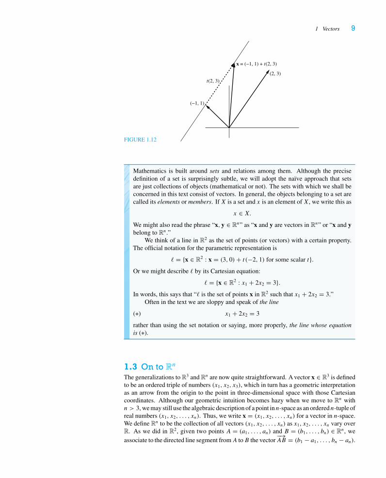
EXAMPLE 4
Consider the line � given in parametric form by
x = (−1, 1)+ t (2, 3)and pictured in Figure 1.12. We wish to find a Cartesian equation of the line. Note that� passes through the point (−1, 1) and has direction vector (2, 3). The direction vectordetermines the slope of the line:
rise
run= 3
2,
so, using the point-slope form of the equation of a line, we find
x2 − 1
x1 + 1= 3
2; i.e., x2 = 3
2x1 + 5
2.
Of course, we can rewrite this as 3x1 − 2x2 = −5.
1 Vectors 9
FIGURE 1.12
t(2, 3)
(2, 3)
x = (−1, 1) + t(2, 3)
(−1, 1)
Mathematics is built around sets and relations among them. Although the precisedefinition of a set is surprisingly subtle, we will adopt the naïve approach that setsare just collections of objects (mathematical or not). The sets with which we shall beconcerned in this text consist of vectors. In general, the objects belonging to a set arecalled its elements or members. IfX is a set and x is an element ofX, we write this as
x ∈ X.We might also read the phrase “x, y ∈ Rn” as “x and y are vectors in Rn” or “x and ybelong to Rn.”
We think of a line in R2 as the set of points (or vectors) with a certain property.The official notation for the parametric representation is
� = {x ∈ R2 : x = (3, 0)+ t (−2, 1) for some scalar t}.Or we might describe � by its Cartesian equation:
� = {x ∈ R2 : x1 + 2x2 = 3}.In words, this says that “� is the set of points x in R2 such that x1 + 2x2 = 3.”
Often in the text we are sloppy and speak of the line
(∗) x1 + 2x2 = 3
rather than using the set notation or saying, more properly, the line whose equationis (∗).
1.3 On to Rn
The generalizations to R3 and Rn are now quite straightforward. A vector x ∈ R3 is definedto be an ordered triple of numbers (x1, x2, x3), which in turn has a geometric interpretationas an arrow from the origin to the point in three-dimensional space with those Cartesiancoordinates. Although our geometric intuition becomes hazy when we move to Rn withn > 3, we may still use the algebraic description of a point inn-space as an orderedn-tuple ofreal numbers (x1, x2, . . . , xn). Thus, we write x = (x1, x2, . . . , xn) for a vector in n-space.We define Rn to be the collection of all vectors (x1, x2, . . . , xn) as x1, x2, . . . , xn vary overR. As we did in R2, given two points A = (a1, . . . , an) and B = (b1, . . . , bn) ∈ Rn, weassociate to the directed line segment fromA toB the vector
−→AB = (b1 − a1, . . . , bn − an).
10 Chapter 1 Vectors and Matrices
Remark. The beginning linear algebra student may wonder why anyone would care about Rn
with n > 3. We hope that the rich structure we’re going to study in this text will eventuallybe satisfying in and of itself. But some will be happier to know that “real-world applications”force the issue, because many applied problems require understanding the interactions ofa large number of variables. For instance, to model the motion of a single particle in R3,we must know the three variables describing its position and the three variables describingits velocity, for a total of six variables. Other examples arise in economic models of alarge number of industries, each of which has a supply-demand equation involving largenumbers of variables, and in population models describing the interaction of large numbersof different species. In these multivariable problems, each variable accounts for one copyof R, and so an n-variable problem naturally leads to linear (and nonlinear) problems in Rn.
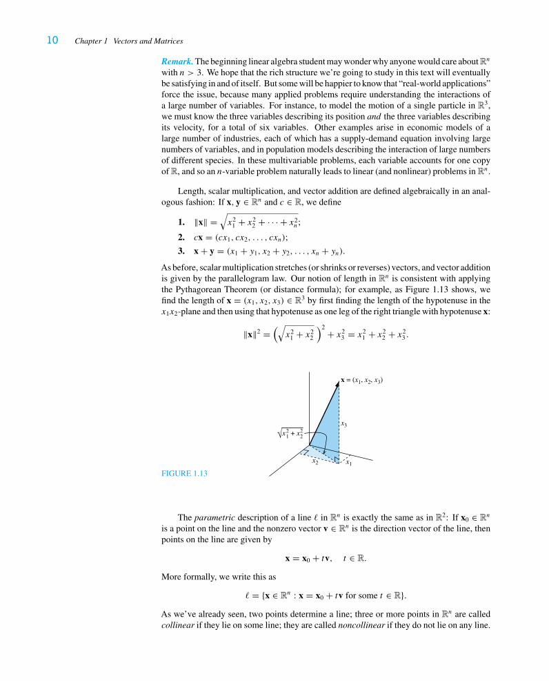
Length, scalar multiplication, and vector addition are defined algebraically in an anal-ogous fashion: If x, y ∈ Rn and c ∈ R, we define
1. ‖x‖ =√x2
1 + x22 + · · · + x2
n;
2. cx = (cx1, cx2, . . . , cxn);
3. x + y = (x1 + y1, x2 + y2, . . . , xn + yn).As before, scalar multiplication stretches (or shrinks or reverses) vectors, and vector additionis given by the parallelogram law. Our notion of length in Rn is consistent with applyingthe Pythagorean Theorem (or distance formula); for example, as Figure 1.13 shows, wefind the length of x = (x1, x2, x3) ∈ R3 by first finding the length of the hypotenuse in thex1x2-plane and then using that hypotenuse as one leg of the right triangle with hypotenuse x:
‖x‖2 =(√x2
1 + x22
)2 + x23 = x2
1 + x22 + x2
3 .
FIGURE 1.13
x2 x1
x3
x = (x1, x2, x3)
√x21 + x2
2
The parametric description of a line � in Rn is exactly the same as in R2: If x0 ∈ Rn
is a point on the line and the nonzero vector v ∈ Rn is the direction vector of the line, thenpoints on the line are given by
x = x0 + tv, t ∈ R.
More formally, we write this as
� = {x ∈ Rn : x = x0 + tv for some t ∈ R}.As we’ve already seen, two points determine a line; three or more points in Rn are calledcollinear if they lie on some line; they are called noncollinear if they do not lie on any line.
1 Vectors 11
EXAMPLE 5
Consider the line determined by the points P = (1, 2, 3) and Q = (2, 1, 5) in R3. Thedirection vector of the line is v = −→
PQ = (2, 1, 5)− (1, 2, 3) = (1,−1, 2), and we get aninitial point x0 = −→
OP , just as we did in R2. We now visualize Figure 1.11 as being in R3
and see that the general point on this line is x = x0 + tv = (1, 2, 3)+ t (1,−1, 2).
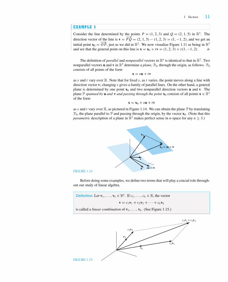
The definition of parallel and nonparallel vectors in Rn is identical to that in R2. Twononparallel vectors u and v in R3 determine a plane, P0, through the origin, as follows. P0
consists of all points of the formx = su + tv
as s and t vary over R. Note that for fixed s, as t varies, the point moves along a line withdirection vector v; changing s gives a family of parallel lines. On the other hand, a generalplane is determined by one point x0 and two nonparallel direction vectors u and v. Theplane P spanned by u and v and passing through the point x0 consists of all points x ∈ R3
of the formx = x0 + su + tv
as s and t vary over R, as pictured in Figure 1.14. We can obtain the plane P by translatingP0, the plane parallel to P and passing through the origin, by the vector x0. (Note that thisparametric description of a plane in R3 makes perfect sense in n-space for any n ≥ 3.)
FIGURE 1.14u
v
x0
x0 + su + tv
su + tv
Before doing some examples, we define two terms that will play a crucial role through-out our study of linear algebra.
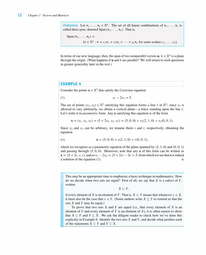
Definition. Let v1, . . . , vk ∈ Rn. If c1, . . . , ck ∈ R, the vector
v = c1v1 + c2v2 + · · · + ckvkis called a linear combination of v1, . . . , vk . (See Figure 1.15.)
FIGURE 1.15
v1
v2
c1v1
c1v1 + c2v2
c2v2
12 Chapter 1 Vectors and Matrices
Definition. Let v1, . . . , vk ∈ Rn. The set of all linear combinations of v1, . . . , vk iscalled their span, denoted Span (v1, . . . , vk). That is,
Span (v1, . . . , vk) ={v ∈ Rn : v = c1v1 + c2v2 + · · · + ckvk for some scalars c1, . . . , ck}.
In terms of our new language, then, the span of two nonparallel vectors u, v ∈ Rn is a planethrough the origin. (What happens if u and v are parallel? We will return to such questionsin greater generality later in the text.)
EXAMPLE 6
Consider the points x ∈ R3 that satisfy the Cartesian equation
(†) x1 − 2x2 = 5.
The set of points (x1, x2) ∈ R2 satisfying this equation forms a line � in R2; since x3 isallowed to vary arbitrarily, we obtain a vertical plane—a fence standing upon the line �.Let’s write it in parametric form: Any x satisfying this equation is of the form
x = (x1, x2, x3) = (5 + 2x2, x2, x3) = (5, 0, 0)+ x2(2, 1, 0)+ x3(0, 0, 1).
Since x2 and x3 can be arbitrary, we rename them s and t , respectively, obtaining theequation
(∗) x = (5, 0, 0)+ s(2, 1, 0)+ t (0, 0, 1),which we recognize as a parametric equation of the plane spanned by (2, 1, 0) and (0, 0, 1)and passing through (5, 0, 0). Moreover, note that any x of this form can be written asx = (5 + 2s, s, t), and sox1 − 2x2 = (5 + 2s)− 2s = 5, from which we see that x is indeeda solution of the equation (†).
This may be an appropriate time to emphasize a basic technique in mathematics: Howdo we decide when two sets are equal? First of all, we say that X is a subset of Y ,written
X ⊂ Y,
if every element ofX is an element of Y . That is,X ⊂ Y means that whenever x ∈ X,it must also be the case that x ∈ Y . (Some authors write X ⊆ Y to remind us that thesets X and Y may be equal.)
To prove that two sets X and Y are equal (i.e., that every element of X is anelement of Y and every element of Y is an element of X), it is often easiest to showthat X ⊂ Y and Y ⊂ X. We ask the diligent reader to check how we’ve done thisexplicitly in Example 6: Identify the two sets X and Y , and decide what justifies eachof the statements X ⊂ Y and Y ⊂ X.
1 Vectors 13
EXAMPLE 7
As was the case for lines, a given plane has many different parametric representations. Forexample,
(∗∗) x = (7, 1,−5)+ u(2, 1, 2)+ v(2, 1, 3)is another description of the plane given in Example 6, as we now proceed to check. First,we ask whether every point of (∗∗) can be expressed in the form of (∗) for some values ofs and t ; that is, fixing u and v, we must find s and t so that
(5, 0, 0)+ s(2, 1, 0)+ t (0, 0, 1) = (7, 1,−5)+ u(2, 1, 2)+ v(2, 1, 3).This gives us the system of equations
2s = 2u+ 2v + 2
s = u+ v + 1
t = 2u+ 3v − 5,
whose solution is obviously s = u+ v + 1 and t = 2u+ 3v − 5. Indeed, we check thealgebra:
(5, 0, 0)+ s(2, 1, 0)+ t (0, 0, 1) = (5, 0, 0)+ (u+ v + 1)(2, 1, 0)
+ (2u+ 3v − 5)(0, 0, 1)
= ((5, 0, 0)+ (2, 1, 0)− 5(0, 0, 1))
+ u((2, 1, 0)+ 2(0, 0, 1))+ v((2, 1, 0)+ 3(0, 0, 1)
)
= (7, 1,−5)+ u(2, 1, 2)+ v(2, 1, 3).In conclusion, every point of (∗∗) does in fact lie in the plane (∗).
Reversing the process is a bit trickier. Given a point of the form (∗) for some fixedvalues of s and t , we need to solve the equations for u and v. We will address this sortof problem in Section 4, but for now, we’ll just notice that if we take u = 3s − t − 8 andv = −2s + t + 7 in the equation (∗∗), we get the point (∗). Thus, every point of the plane(∗) lies in the plane (∗∗). This means the two planes are, in fact, identical.
EXAMPLE 8
Consider the points x ∈ R3 that satisfy the equation
x1 − 2x2 + x3 = 5.
Any x satisfying this equation is of the form
x = (x1, x2, x3) = (5 + 2x2 − x3, x2, x3) = (5, 0, 0)+ x2(2, 1, 0)+ x3(−1, 0, 1).
So this equation describes a plane P spanned by (2, 1, 0) and (−1, 0, 1) and passing through(5, 0, 0). We leave it to the reader to check the converse—that every point in the plane P
satisfies the original Cartesian equation.
In the preceding examples, we started with a Cartesian equation of a plane in R3 andderived a parametric formulation. Of course, planes can be described in different ways.
14 Chapter 1 Vectors and Matrices
EXAMPLE 9
We wish to find a parametric equation of the plane that contains the points P = (1, 2, 1)andQ = (2, 4, 0) and is parallel to the vector (1, 1, 3). We take x0 = (1, 2, 1), u = −→
PQ =(1, 2,−1), and v = (1, 1, 3), so the plane consists of all points of the form
x = (1, 2, 1)+ s(1, 2,−1)+ t (1, 1, 3), s, t ∈ R.
Finally, note that three noncollinear points P,Q,R ∈ R3 determine a plane. To get aparametric equation of this plane, we simply take x0 = −→
OP , u = −→PQ, and v = −→
PR. Weshould observe that if P ,Q, and R are noncollinear, then u and v are nonparallel (why?).
It is also a reasonable question to ask whether a specific point lies on a given plane.
EXAMPLE 10
Let u = (1, 1, 0,−1) and v = (2, 0, 1, 1). We ask whether the vector x = (1, 3,−1,−2)is a linear combination of u and v. That is, are there scalars s and t so that su + tv = x,i.e.,
s(1, 1, 0,−1)+ t (2, 0, 1, 1) = (1, 3,−1,−2)?
Expanding, we have
(s + 2t, s, t,−s + t) = (1, 3,−1,−2),
which leads to the system of equations
s + 2t = 1
s = 3
t = −1
−s + t = −2 .
From the second and third equations we infer that s = 3 and t = −1. These values alsosatisfy the first equation, but not the fourth, and so the system of equations has no solution;that is, there are no values of s and t for which all the equations hold. Thus, x is not alinear combination of u and v. Geometrically, this means that the vector x does not lie inthe plane spanned by u and v and passing through the origin. We will learn a systematicway of solving such systems of linear equations in Section 4.
EXAMPLE 11
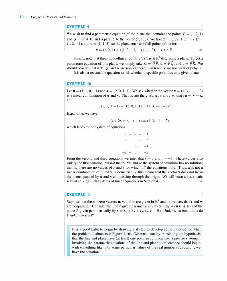
Suppose that the nonzero vectors u, v, and w are given in R3 and, moreover, that v and ware nonparallel. Consider the line � given parametrically by x = x0 + ru (r ∈ R) and theplane P given parametrically by x = x1 + sv + tw (s, t,∈ R). Under what conditions do� and P intersect?
It is a good habit to begin by drawing a sketch to develop some intuition for whatthe problem is about (see Figure 1.16). We must start by translating the hypothesisthat the line and plane have (at least) one point in common into a precise statementinvolving the parametric equations of the line and plane; our sentence should beginwith something like “For some particular values of the real numbers r , s, and t , wehave the equation . . . .”
1 Vectors 15
FIGURE 1.16
x1x0
u wv
�
P
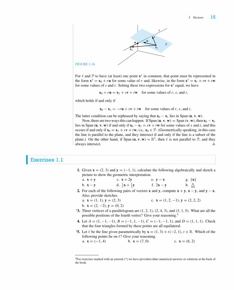
For � and P to have (at least) one point x∗ in common, that point must be represented inthe form x∗ = x0 + ru for some value of r and, likewise, in the form x∗ = x1 + sv + twfor some values of s and t . Setting these two expressions for x∗ equal, we have
x0 + ru = x1 + sv + tw for some values of r , s, and t ,
which holds if and only if
x0 − x1 = −ru + sv + tw for some values of r , s, and t .
The latter condition can be rephrased by saying that x0 − x1 lies in Span (u, v,w).Now, there are two ways this can happen. If Span (u, v,w) = Span (v,w), then x0 − x1
lies in Span (u, v,w) if and only if x0 − x1 = sv + tw for some values of s and t , and thisoccurs if and only if x0 = x1 + sv + tw, i.e., x0 ∈ P. (Geometrically speaking, in this casethe line is parallel to the plane, and they intersect if and only if the line is a subset of theplane.) On the other hand, if Span (u, v,w) = R3, then � is not parallel to P, and theyalways intersect.
Exercises 1.1
1. Given x = (2, 3) and y = (−1, 1), calculate the following algebraically and sketch apicture to show the geometric interpretation.a. x + yb. x − y
c. x + 2yd. 1
2 x + 12 y
e. y − xf. 2x − y
g. ‖x‖h. x
‖x‖2. For each of the following pairs of vectors x and y, compute x + y, x − y, and y − x.
Also, provide sketches.a. x = (1, 1), y = (2, 3)
b. x = (2,−2), y = (0, 2)
c. x = (1, 2,−1), y = (2, 2, 2)
3.∗ Three vertices of a parallelogram are (1, 2, 1), (2, 4, 3), and (3, 1, 5). What are all thepossible positions of the fourth vertex? Give your reasoning.4
4. Let A = (1,−1,−1), B = (−1, 1,−1), C = (−1,−1, 1), and D = (1, 1, 1). Checkthat the four triangles formed by these points are all equilateral.
5.∗ Let � be the line given parametrically by x = (1, 3)+ t (−2, 1), t ∈ R. Which of thefollowing points lie on �? Give your reasoning.a. x = (−1, 4) b. x = (7, 0) c. x = (6, 2)
4For exercises marked with an asterisk (*) we have provided either numerical answers or solutions at the back ofthe book.
16 Chapter 1 Vectors and Matrices
6. Find a parametric equation of each of the following lines:a. 3x1 + 4x2 = 6
b.∗ the line with slope 1/3 that passes through A = (−1, 2)
c. the line with slope 2/5 that passes through A = (3, 1)
d. the line through A = (−2, 1) parallel to x = (1, 4)+ t (3, 5)e. the line through A = (−2, 1) perpendicular to x = (1, 4)+ t (3, 5)f.∗ the line through A = (1, 2, 1) and B = (2, 1, 0)
g. the line through A = (1,−2, 1) and B = (2, 1,−1)
h.∗ the line through (1, 1, 0,−1) parallel to x = (2 + t, 1 − 2t, 3t, 4 − t)7. Suppose x = x0 + tv and y = y0 + sw are two parametric representations of the same
line � in Rn.a. Show that there is a scalar t0 so that y0 = x0 + t0v.
b. Show that v and w are parallel.
8.∗ Decide whether each of the following vectors is a linear combination of u = (1, 0, 1)and v = (−2, 1, 0).a. x = (1, 0, 0) b. x = (3,−1, 1) c. x = (0, 1, 2)
9.∗ Let P be the plane in R3 spanned by u = (1, 1, 0) and v = (1,−1, 1) and passingthrough the point (3, 0,−2). Which of the following points lie on P?a. x = (4,−1,−1)
b. x = (1,−1, 1)
c. x = (7,−2, 1)
d. x = (5, 2, 0)
10. Find a parametric equation of each of the following planes:a. the plane containing the point (−1, 0, 1) and the line x = (1, 1, 1)+ t (1, 7,−1)
b.∗ the plane parallel to the vector (1, 3, 1) and containing the points (1, 1, 1) and(−2, 1, 2)
c. the plane containing the points (1, 1, 2), (2, 3, 4), and (0,−1, 2)
d. the plane in R4 containing the points (1, 1,−1, 2), (2, 3, 0, 1), and (1, 2, 2, 3)
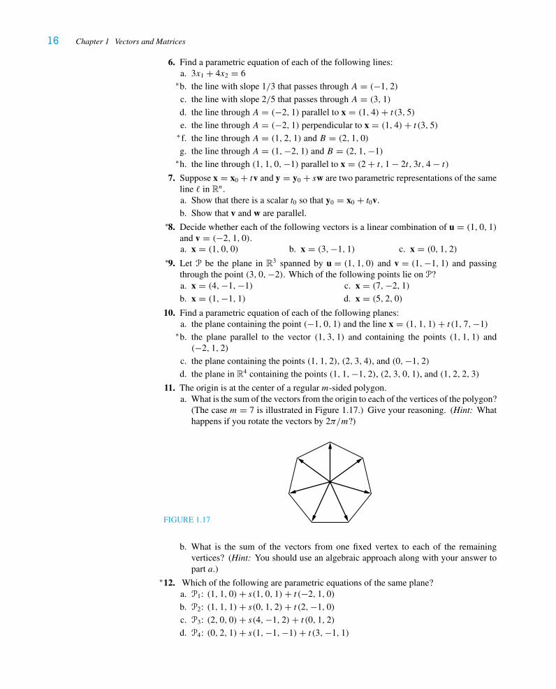
11. The origin is at the center of a regular m-sided polygon.a. What is the sum of the vectors from the origin to each of the vertices of the polygon?
(The case m = 7 is illustrated in Figure 1.17.) Give your reasoning. (Hint: Whathappens if you rotate the vectors by 2π/m?)
FIGURE 1.17
b. What is the sum of the vectors from one fixed vertex to each of the remainingvertices? (Hint: You should use an algebraic approach along with your answer topart a.)
12.∗ Which of the following are parametric equations of the same plane?a. P1: (1, 1, 0)+ s(1, 0, 1)+ t (−2, 1, 0)
b. P2: (1, 1, 1)+ s(0, 1, 2)+ t (2,−1, 0)
c. P3: (2, 0, 0)+ s(4,−1, 2)+ t (0, 1, 2)d. P4: (0, 2, 1)+ s(1,−1,−1)+ t (3,−1, 1)
1 Vectors 17
13. Given �ABC, letM and N be the midpoints of AB and AC, respectively. Prove that−−→MN = 1
2
−→BC.
14. Let ABCD be an arbitrary quadrilateral. Let P , Q, R, and S be the midpoints ofAB, BC, CD, and DA, respectively. Use Exercise 13 to prove that PQRS is aparallelogram.
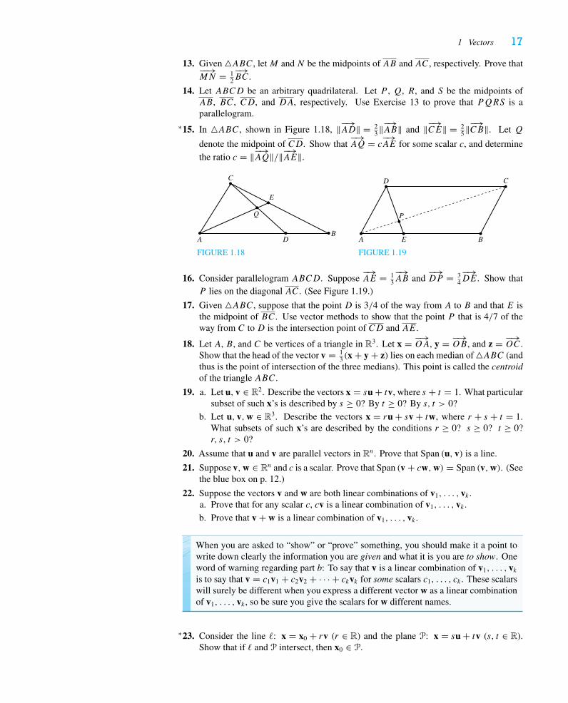
15.∗ In �ABC, shown in Figure 1.18, ‖−→AD‖ = 23‖−→AB‖ and ‖−→CE‖ = 2
5‖−→CB‖. Let Q
denote the midpoint of CD. Show that−→AQ = c
−→AE for some scalar c, and determine
the ratio c = ‖−→AQ‖/‖−→AE‖.
AB
C
D
E
Q
FIGURE 1.18
A B
CD
E
P
FIGURE 1.19
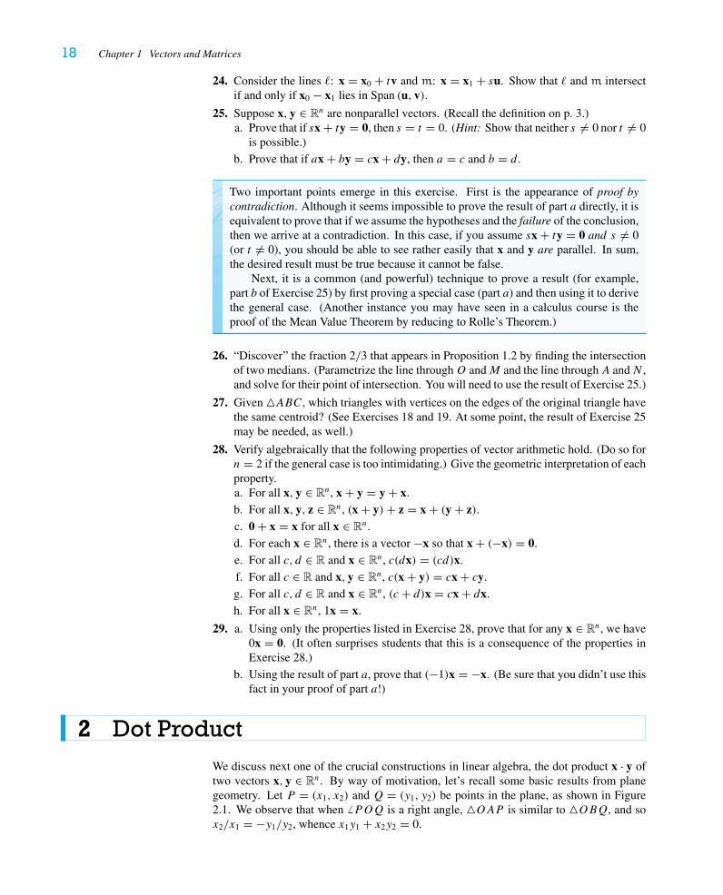
16. Consider parallelogram ABCD. Suppose−→AE = 1
3
−→AB and
−→DP = 3
4
−→DE. Show that
P lies on the diagonal AC. (See Figure 1.19.)
17. Given �ABC, suppose that the point D is 3/4 of the way from A to B and that E isthe midpoint of BC. Use vector methods to show that the point P that is 4/7 of theway from C to D is the intersection point of CD and AE.
18. Let A, B, and C be vertices of a triangle in R3. Let x = −→OA, y = −→
OB, and z = −→OC.
Show that the head of the vector v = 13 (x + y + z) lies on each median of �ABC (and
thus is the point of intersection of the three medians). This point is called the centroidof the triangle ABC.
19. a. Let u, v ∈ R2. Describe the vectors x = su + tv, where s + t = 1. What particularsubset of such x’s is described by s ≥ 0? By t ≥ 0? By s, t > 0?
b. Let u, v,w ∈ R3. Describe the vectors x = ru + sv + tw, where r + s + t = 1.What subsets of such x’s are described by the conditions r ≥ 0? s ≥ 0? t ≥ 0?r, s, t > 0?
20. Assume that u and v are parallel vectors in Rn. Prove that Span (u, v) is a line.
21. Suppose v,w ∈ Rn and c is a scalar. Prove that Span (v + cw,w) = Span (v,w). (Seethe blue box on p. 12.)
22. Suppose the vectors v and w are both linear combinations of v1, . . . , vk .a. Prove that for any scalar c, cv is a linear combination of v1, . . . , vk .b. Prove that v + w is a linear combination of v1, . . . , vk .
When you are asked to “show” or “prove” something, you should make it a point towrite down clearly the information you are given and what it is you are to show. Oneword of warning regarding part b: To say that v is a linear combination of v1, . . . , vkis to say that v = c1v1 + c2v2 + · · · + ckvk for some scalars c1, . . . , ck . These scalarswill surely be different when you express a different vector w as a linear combinationof v1, . . . , vk , so be sure you give the scalars for w different names.
23.∗ Consider the line �: x = x0 + rv (r ∈ R) and the plane P: x = su + tv (s, t ∈ R).Show that if � and P intersect, then x0 ∈ P.
18 Chapter 1 Vectors and Matrices
24. Consider the lines �: x = x0 + tv and m: x = x1 + su. Show that � and m intersectif and only if x0 − x1 lies in Span (u, v).
25. Suppose x, y ∈ Rn are nonparallel vectors. (Recall the definition on p. 3.)a. Prove that if sx + ty = 0, then s = t = 0. (Hint: Show that neither s �= 0 nor t �= 0
is possible.)
b. Prove that if ax + by = cx + dy, then a = c and b = d.
Two important points emerge in this exercise. First is the appearance of proof bycontradiction. Although it seems impossible to prove the result of part a directly, it isequivalent to prove that if we assume the hypotheses and the failure of the conclusion,then we arrive at a contradiction. In this case, if you assume sx + ty = 0 and s �= 0(or t �= 0), you should be able to see rather easily that x and y are parallel. In sum,the desired result must be true because it cannot be false.
Next, it is a common (and powerful) technique to prove a result (for example,part b of Exercise 25) by first proving a special case (part a) and then using it to derivethe general case. (Another instance you may have seen in a calculus course is theproof of the Mean Value Theorem by reducing to Rolle’s Theorem.)
26. “Discover” the fraction 2/3 that appears in Proposition 1.2 by finding the intersectionof two medians. (Parametrize the line throughO andM and the line throughA andN ,and solve for their point of intersection. You will need to use the result of Exercise 25.)
27. Given �ABC, which triangles with vertices on the edges of the original triangle havethe same centroid? (See Exercises 18 and 19. At some point, the result of Exercise 25may be needed, as well.)
28. Verify algebraically that the following properties of vector arithmetic hold. (Do so forn = 2 if the general case is too intimidating.) Give the geometric interpretation of eachproperty.a. For all x, y ∈ Rn, x + y = y + x.
b. For all x, y, z ∈ Rn, (x + y)+ z = x + (y + z).c. 0 + x = x for all x ∈ Rn.
d. For each x ∈ Rn, there is a vector −x so that x + (−x) = 0.
e. For all c, d ∈ R and x ∈ Rn, c(dx) = (cd)x.
f. For all c ∈ R and x, y ∈ Rn, c(x + y) = cx + cy.
g. For all c, d ∈ R and x ∈ Rn, (c + d)x = cx + dx.
h. For all x ∈ Rn, 1x = x.
29. a. Using only the properties listed in Exercise 28, prove that for any x ∈ Rn, we have0x = 0. (It often surprises students that this is a consequence of the properties inExercise 28.)
b. Using the result of part a, prove that (−1)x = −x. (Be sure that you didn’t use thisfact in your proof of part a!)
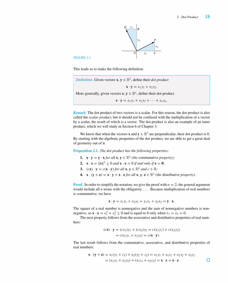
2 Dot ProductWe discuss next one of the crucial constructions in linear algebra, the dot product x · y oftwo vectors x, y ∈ Rn. By way of motivation, let’s recall some basic results from planegeometry. Let P = (x1, x2) and Q = (y1, y2) be points in the plane, as shown in Figure2.1. We observe that when � POQ is a right angle, �OAP is similar to �OBQ, and sox2/x1 = −y1/y2, whence x1y1 + x2y2 = 0.
2 Dot Product 19
FIGURE 2.1
P
Q
O
x2
A
B
x1
y1
y2
This leads us to make the following definition.
Definition. Given vectors x, y ∈ R2, define their dot product
x · y = x1y1 + x2y2.
More generally, given vectors x, y ∈ Rn, define their dot product
x · y = x1y1 + x2y2 + · · · + xnyn.
Remark. The dot product of two vectors is a scalar. For this reason, the dot product is alsocalled the scalar product, but it should not be confused with the multiplication of a vectorby a scalar, the result of which is a vector. The dot product is also an example of an innerproduct, which we will study in Section 6 of Chapter 3.
We know that when the vectors x and y ∈ R2 are perpendicular, their dot product is 0.By starting with the algebraic properties of the dot product, we are able to get a great dealof geometry out of it.
Proposition 2.1. The dot product has the following properties:
1. x · y = y · x for all x, y ∈ Rn (the commutative property);
2. x · x = ‖x‖2 ≥ 0 and x · x = 0 if and only if x = 0;
3. (cx) · y = c(x · y) for all x, y ∈ Rn and c ∈ R;
4. x · (y + z) = x · y + x · z for all x, y, z ∈ Rn (the distributive property).
Proof. In order to simplify the notation, we give the proof with n = 2; the general argumentwould include all n terms with the obligatory . . . . Because multiplication of real numbersis commutative, we have
x · y = x1y1 + x2y2 = y1x1 + y2x2 = y · x.
The square of a real number is nonnegative and the sum of nonnegative numbers is non-negative, so x · x = x2
1 + x22 ≥ 0 and is equal to 0 only when x1 = x2 = 0.
The next property follows from the associative and distributive properties of real num-bers:
(cx) · y = (cx1)y1 + (cx2)y2 = c(x1y1)+ c(x2y2)
= c(x1y1 + x2y2) = c(x · y).
The last result follows from the commutative, associative, and distributive properties ofreal numbers:
x · (y + z) = x1(y1 + z1)+ x2(y2 + z2) = x1y1 + x1z1 + x2y2 + x2z2
= (x1y1 + x2y2)+ (x1z1 + x2z2) = x · y + x · z.
20 Chapter 1 Vectors and Matrices
Corollary 2.2. ‖x + y‖2 = ‖x‖2 + 2x · y + ‖y‖2.
Proof. Using the properties of Proposition 2.1 repeatedly, we have
‖x + y‖2 = (x + y) · (x + y)
= x · x + x · y + y · x + y · y
= ‖x‖2 + 2x · y + ‖y‖2,
as desired.
Although we use coordinates to define the dot product and to derive its algebraicproperties in Proposition 2.1, from this point on we should try to use the propertiesthemselves to prove results (e.g., Corollary 2.2). This will tend to avoid an algebraicmess and emphasize the geometry.
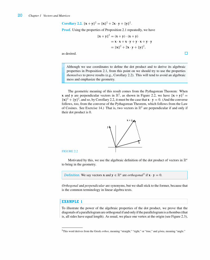
The geometric meaning of this result comes from the Pythagorean Theorem: Whenx and y are perpendicular vectors in R2, as shown in Figure 2.2, we have ‖x + y‖2 =‖x‖2 + ‖y‖2, and so, by Corollary 2.2, it must be the case that x · y = 0. (And the conversefollows, too, from the converse of the Pythagorean Theorem, which follows from the Lawof Cosines. See Exercise 14.) That is, two vectors in R2 are perpendicular if and only iftheir dot product is 0.
FIGURE 2.2
x
x + y
y
Motivated by this, we use the algebraic definition of the dot product of vectors in Rn
to bring in the geometry.
Definition. We say vectors x and y ∈ Rn are orthogonal5 if x · y = 0.
Orthogonal and perpendicular are synonyms, but we shall stick to the former, because thatis the common terminology in linear algebra texts.
EXAMPLE 1
To illustrate the power of the algebraic properties of the dot product, we prove that thediagonals of a parallelogram are orthogonal if and only if the parallelogram is a rhombus (thatis, all sides have equal length). As usual, we place one vertex at the origin (see Figure 2.3),
5This word derives from the Greek orthos, meaning “straight,” “right,” or “true,” and gonia, meaning “angle.”
2 Dot Product 21
FIGURE 2.3
Ax
y
x − y
x + yCB
O
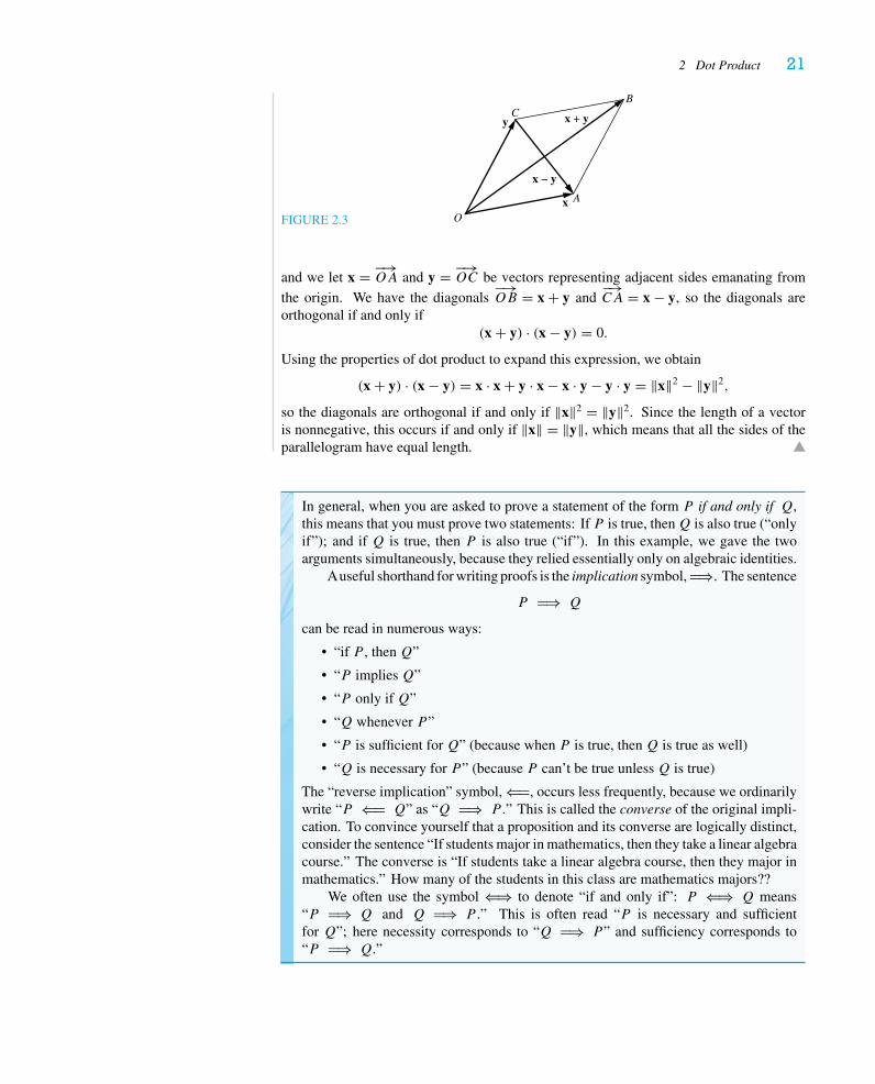
and we let x = −→OA and y = −→
OC be vectors representing adjacent sides emanating fromthe origin. We have the diagonals
−→OB = x + y and
−→CA = x − y, so the diagonals are
orthogonal if and only if(x + y) · (x − y) = 0.
Using the properties of dot product to expand this expression, we obtain
(x + y) · (x − y) = x · x + y · x − x · y − y · y = ‖x‖2 − ‖y‖2,
so the diagonals are orthogonal if and only if ‖x‖2 = ‖y‖2. Since the length of a vectoris nonnegative, this occurs if and only if ‖x‖ = ‖y‖, which means that all the sides of theparallelogram have equal length.
In general, when you are asked to prove a statement of the form P if and only if Q,this means that you must prove two statements: If P is true, thenQ is also true (“onlyif”); and if Q is true, then P is also true (“if”). In this example, we gave the twoarguments simultaneously, because they relied essentially only on algebraic identities.
Auseful shorthand for writing proofs is the implication symbol, �⇒. The sentence
P �⇒ Q
can be read in numerous ways:
• “if P , thenQ”
• “P impliesQ”
• “P only ifQ”
• “Q whenever P ”
• “P is sufficient forQ” (because when P is true, thenQ is true as well)
• “Q is necessary for P ” (because P can’t be true unlessQ is true)
The “reverse implication” symbol, ⇐�, occurs less frequently, because we ordinarilywrite “P ⇐� Q” as “Q �⇒ P .” This is called the converse of the original impli-cation. To convince yourself that a proposition and its converse are logically distinct,consider the sentence “If students major in mathematics, then they take a linear algebracourse.” The converse is “If students take a linear algebra course, then they major inmathematics.” How many of the students in this class are mathematics majors??
We often use the symbol ⇐⇒ to denote “if and only if”: P ⇐⇒ Q means“P �⇒ Q and Q �⇒ P .” This is often read “P is necessary and sufficientfor Q”; here necessity corresponds to “Q �⇒ P ” and sufficiency corresponds to“P �⇒ Q.”
22 Chapter 1 Vectors and Matrices
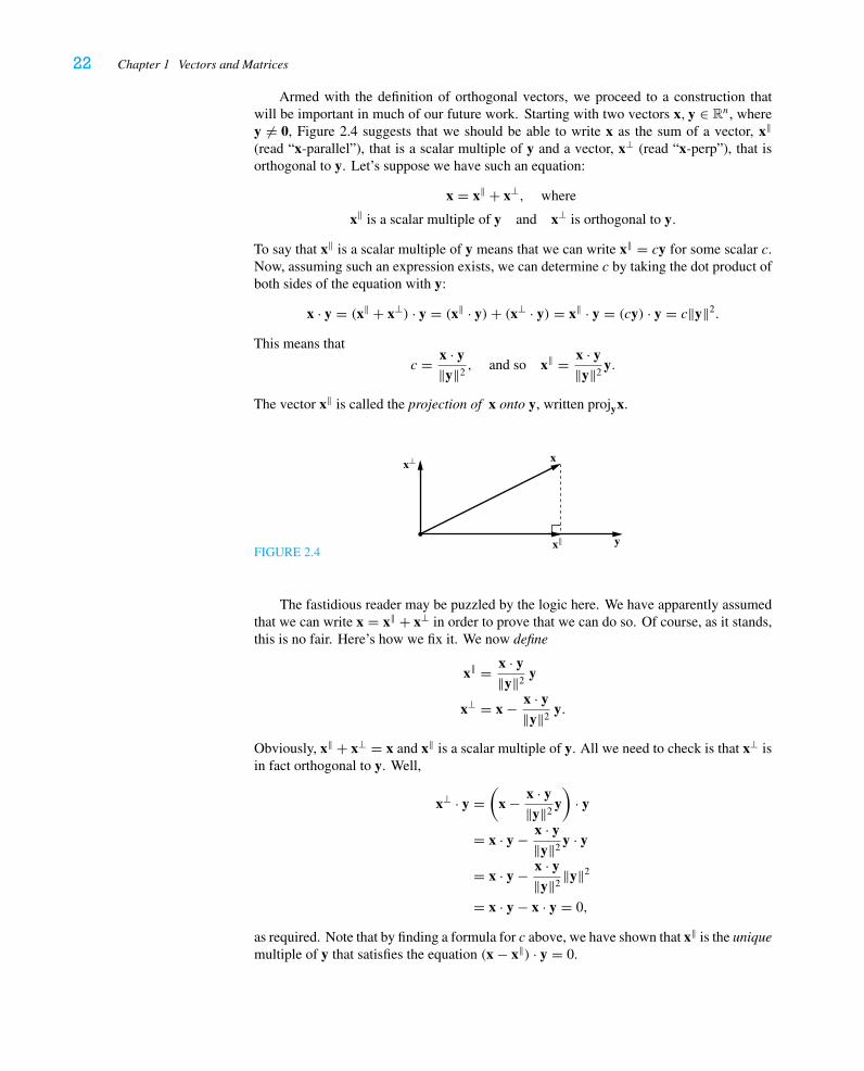
Armed with the definition of orthogonal vectors, we proceed to a construction thatwill be important in much of our future work. Starting with two vectors x, y ∈ Rn, wherey �= 0, Figure 2.4 suggests that we should be able to write x as the sum of a vector, x‖(read “x-parallel”), that is a scalar multiple of y and a vector, x⊥ (read “x-perp”), that isorthogonal to y. Let’s suppose we have such an equation:
x = x‖ + x⊥, where
x‖ is a scalar multiple of y and x⊥ is orthogonal to y.
To say that x‖ is a scalar multiple of y means that we can write x‖ = cy for some scalar c.Now, assuming such an expression exists, we can determine c by taking the dot product ofboth sides of the equation with y:
x · y = (x‖ + x⊥) · y = (x‖ · y)+ (x⊥ · y) = x‖ · y = (cy) · y = c‖y‖2.
This means that
c = x · y‖y‖2
, and so x‖ = x · y‖y‖2
y.
The vector x‖ is called the projection of x onto y, written projyx.
FIGURE 2.4
x
yx‖
x⊥
The fastidious reader may be puzzled by the logic here. We have apparently assumedthat we can write x = x‖ + x⊥ in order to prove that we can do so. Of course, as it stands,this is no fair. Here’s how we fix it. We now define
x‖ = x · y‖y‖2
y
x⊥ = x − x · y‖y‖2
y.
Obviously, x‖ + x⊥ = x and x‖ is a scalar multiple of y. All we need to check is that x⊥ isin fact orthogonal to y. Well,
x⊥ · y =(
x − x · y‖y‖2
y)
· y
= x · y − x · y‖y‖2
y · y
= x · y − x · y‖y‖2
‖y‖2
= x · y − x · y = 0,
as required. Note that by finding a formula for c above, we have shown that x‖ is the uniquemultiple of y that satisfies the equation (x − x‖) · y = 0.
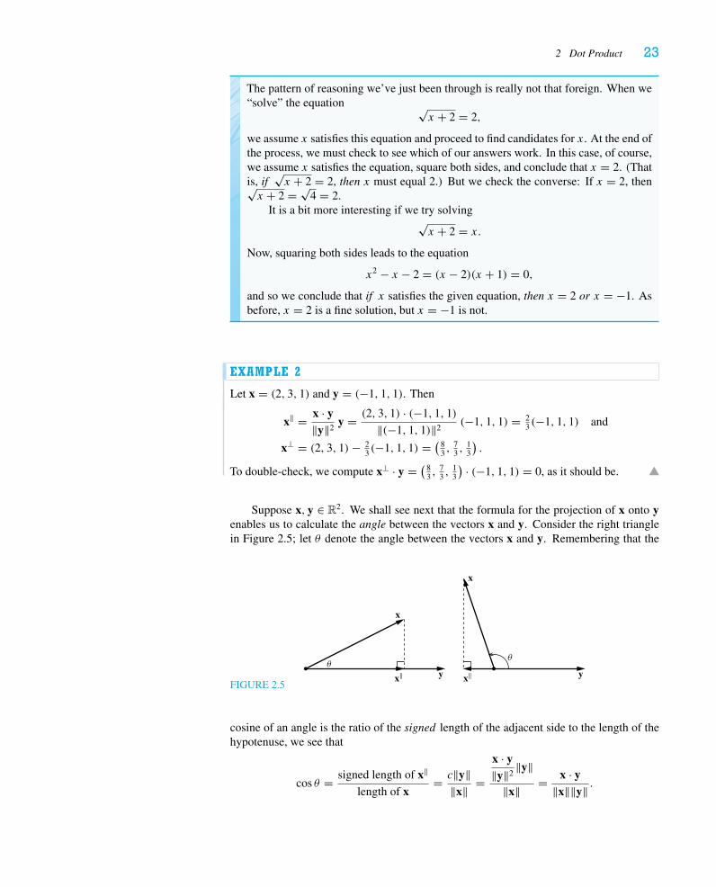
2 Dot Product 23
The pattern of reasoning we’ve just been through is really not that foreign. When we“solve” the equation √
x + 2 = 2,
we assume x satisfies this equation and proceed to find candidates for x. At the end ofthe process, we must check to see which of our answers work. In this case, of course,we assume x satisfies the equation, square both sides, and conclude that x = 2. (Thatis, if
√x + 2 = 2, then x must equal 2.) But we check the converse: If x = 2, then√
x + 2 = √4 = 2.
It is a bit more interesting if we try solving√x + 2 = x.
Now, squaring both sides leads to the equation
x2 − x − 2 = (x − 2)(x + 1) = 0,
and so we conclude that if x satisfies the given equation, then x = 2 or x = −1. Asbefore, x = 2 is a fine solution, but x = −1 is not.
EXAMPLE 2
Let x = (2, 3, 1) and y = (−1, 1, 1). Then
x‖ = x · y‖y‖2
y = (2, 3, 1) · (−1, 1, 1)
‖(−1, 1, 1)‖2(−1, 1, 1) = 2
3 (−1, 1, 1) and
x⊥ = (2, 3, 1)− 23 (−1, 1, 1) = ( 8
3 ,73 ,
13
).
To double-check, we compute x⊥ · y = ( 83 ,
73 ,
13
) · (−1, 1, 1) = 0, as it should be.
Suppose x, y ∈ R2. We shall see next that the formula for the projection of x onto yenables us to calculate the angle between the vectors x and y. Consider the right trianglein Figure 2.5; let θ denote the angle between the vectors x and y. Remembering that the
FIGURE 2.5y y
x
x
x‖ x‖θ
θ
cosine of an angle is the ratio of the signed length of the adjacent side to the length of thehypotenuse, we see that
cos θ = signed length of x‖
length of x= c‖y‖
‖x‖ =x · y‖y‖2
‖y‖‖x‖ = x · y
‖x‖‖y‖ .
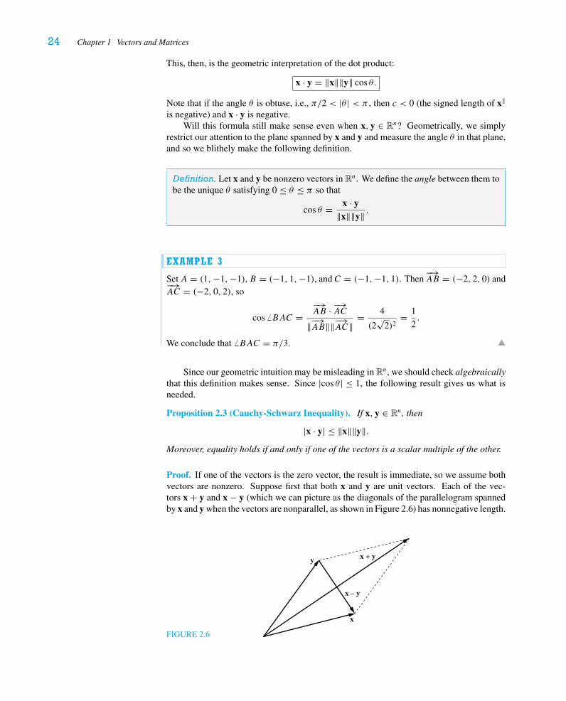
24 Chapter 1 Vectors and Matrices
This, then, is the geometric interpretation of the dot product:
x · y = ‖x‖‖y‖ cos θ.
Note that if the angle θ is obtuse, i.e., π/2 < |θ | < π , then c < 0 (the signed length of x‖is negative) and x · y is negative.
Will this formula still make sense even when x, y ∈ Rn? Geometrically, we simplyrestrict our attention to the plane spanned by x and y and measure the angle θ in that plane,and so we blithely make the following definition.
Definition. Let x and y be nonzero vectors in Rn. We define the angle between them tobe the unique θ satisfying 0 ≤ θ ≤ π so that
cos θ = x · y‖x‖‖y‖ .
EXAMPLE 3
SetA = (1,−1,−1), B = (−1, 1,−1), andC = (−1,−1, 1). Then−→AB = (−2, 2, 0) and−→
AC = (−2, 0, 2), so
cos � BAC =−→AB · −→
AC
‖−→AB‖‖−→AC‖= 4
(2√
2)2= 1
2.
We conclude that � BAC = π/3.
Since our geometric intuition may be misleading in Rn, we should check algebraicallythat this definition makes sense. Since |cos θ | ≤ 1, the following result gives us what isneeded.
Proposition 2.3 (Cauchy-Schwarz Inequality). If x, y ∈ Rn, then
|x · y| ≤ ‖x‖‖y‖.Moreover, equality holds if and only if one of the vectors is a scalar multiple of the other.
Proof. If one of the vectors is the zero vector, the result is immediate, so we assume bothvectors are nonzero. Suppose first that both x and y are unit vectors. Each of the vec-tors x + y and x − y (which we can picture as the diagonals of the parallelogram spannedby x and y when the vectors are nonparallel, as shown in Figure 2.6) has nonnegative length.
FIGURE 2.6
x
x + y
x – y
y
2 Dot Product 25
Using Corollary 2.2, we have
‖x + y‖2 = ‖x‖2 + 2x · y + ‖y‖2 = 2(x · y + 1)
‖x − y‖2 = ‖x‖2 − 2x · y + ‖y‖2 = 2(−x · y + 1).
Since ‖x + y‖2 ≥ 0 and ‖x − y‖2 ≥ 0, we see that x · y + 1 ≥ 0 and −x · y + 1 ≥ 0. Thus,
−1 ≤ x · y ≤ 1, and so |x · y| ≤ 1.
Note that equality holds if and only if either x + y = 0 or x − y = 0, i.e., if and only ifx = ±y.
In general, since x/‖x‖ and y/‖y‖ are unit vectors, we have∣∣∣∣
x‖x‖ · y
‖y‖∣∣∣∣ ≤ 1, and so |x · y| ≤ ‖x‖‖y‖,
as required. Equality holds if and only ifx
‖x‖ = ± y‖y‖ ; that is, equality holds if and only
if x and y are parallel.
Remark. The dot product also arises in situations removed from geometry. The economistintroduces the commodity vector, whose entries are the quantities of various commoditiesthat happen to be of interest. For example, we might consider x = (x1, x2, x3, x4, x5) ∈ R5,where x1 represents the number of pounds of flour, x2 the number of dozens of eggs, x3
the number of pounds of chocolate chips, x4 the number of pounds of walnuts, and x5 thenumber of pounds of butter needed to produce a certain massive quantity of chocolate chipcookies. The economist next introduces the price vector p = (p1, p2, p3, p4, p5) ∈ R5,where pi is the price (in dollars) of a unit of the i th commodity (for example, p2 is the priceof a dozen eggs). Then it follows that
p · x = p1x1 + p2x2 + p3x3 + p4x4 + p5x5
is the total cost of producing the massive quantity of cookies. (To be realistic, we mightalso want to include x6 as the number of hours of labor, with corresponding hourly wagep6.) We will return to this interpretation in Section 5 of Chapter 2.
The gambler uses the dot product to compute the expected value of a lottery that hasmultiple payoffs with various probabilities. If the possible payoffs for a given lotteryare given by w = (w1, . . . , wn) and the probabilities of winning the respective payoffsare given by p = (p1, . . . , pn), with p1 + · · · + pn = 1, then the expected value of thelottery is p · w = p1w1 + · · · + pnwn. For example, if the possible prizes, in dollars, for aparticular lottery are given by the payoff vector w = (0, 1, 5, 100) and the probability vectoris p = (0.5, 0.4, 0.09, 0.01), then the expected value is p · w = 0.4 + 0.45 + 1 = 1.85.Thus, if the lottery ticket costs more than $1.85, the gambler should expect to lose moneyin the long run.
Exercises 1.2
1. For each of the following pairs of vectors x and y, calculate x · y and the angle θbetween the vectors.
a. x = (2, 5), y = (−5, 2)
b. x = (2, 1), y = (−1, 1)
c.∗ x = (1, 8), y = (7,−4)
d. x = (1, 4,−3), y = (5, 1, 3)
e. x = (1,−1, 6), y = (5, 3, 2)
f.∗ x = (3,−4, 5), y = (−1, 0, 1)
g. x = (1, 1, 1, 1), y = (1,−3,−1, 5)
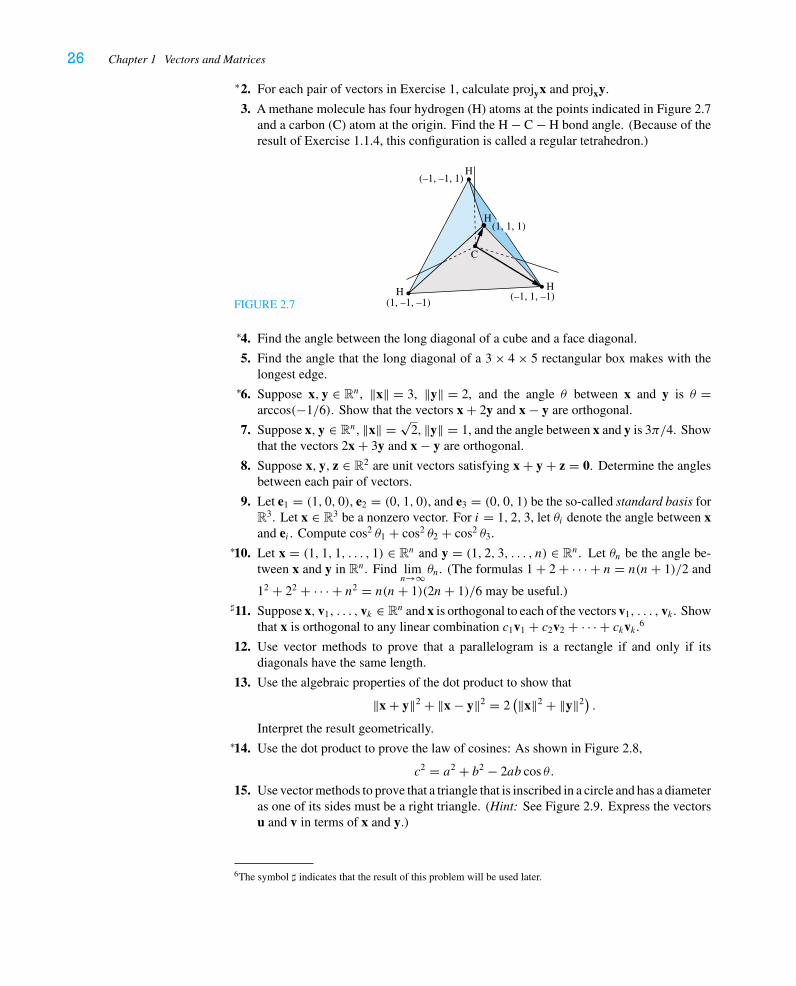
26 Chapter 1 Vectors and Matrices
2.∗ For each pair of vectors in Exercise 1, calculate projyx and projxy.
3. A methane molecule has four hydrogen (H) atoms at the points indicated in Figure 2.7and a carbon (C) atom at the origin. Find the H − C − H bond angle. (Because of theresult of Exercise 1.1.4, this configuration is called a regular tetrahedron.)
FIGURE 2.7
C
H
H
HH
(1, 1, 1)
(–1, 1, –1)(1, –1, –1)
(–1, –1, 1)
4.∗ Find the angle between the long diagonal of a cube and a face diagonal.
5. Find the angle that the long diagonal of a 3 × 4 × 5 rectangular box makes with thelongest edge.
6.∗ Suppose x, y ∈ Rn, ‖x‖ = 3, ‖y‖ = 2, and the angle θ between x and y is θ =arccos(−1/6). Show that the vectors x + 2y and x − y are orthogonal.
7. Suppose x, y ∈ Rn, ‖x‖ = √2, ‖y‖ = 1, and the angle between x and y is 3π/4. Show
that the vectors 2x + 3y and x − y are orthogonal.
8. Suppose x, y, z ∈ R2 are unit vectors satisfying x + y + z = 0. Determine the anglesbetween each pair of vectors.
9. Let e1 = (1, 0, 0), e2 = (0, 1, 0), and e3 = (0, 0, 1) be the so-called standard basis forR3. Let x ∈ R3 be a nonzero vector. For i = 1, 2, 3, let θi denote the angle between xand ei . Compute cos2 θ1 + cos2 θ2 + cos2 θ3.
10.∗ Let x = (1, 1, 1, . . . , 1) ∈ Rn and y = (1, 2, 3, . . . , n) ∈ Rn. Let θn be the angle be-tween x and y in Rn. Find lim
n→∞ θn. (The formulas 1 + 2 + · · · + n = n(n+ 1)/2 and
12 + 22 + · · · + n2 = n(n+ 1)(2n+ 1)/6 may be useful.)
11.� Suppose x, v1, . . . , vk ∈ Rn and x is orthogonal to each of the vectors v1, . . . , vk . Showthat x is orthogonal to any linear combination c1v1 + c2v2 + · · · + ckvk .6
12. Use vector methods to prove that a parallelogram is a rectangle if and only if itsdiagonals have the same length.
13. Use the algebraic properties of the dot product to show that
‖x + y‖2 + ‖x − y‖2 = 2(‖x‖2 + ‖y‖2
).
Interpret the result geometrically.
14.∗ Use the dot product to prove the law of cosines: As shown in Figure 2.8,
c2 = a2 + b2 − 2ab cos θ.
15. Use vector methods to prove that a triangle that is inscribed in a circle and has a diameteras one of its sides must be a right triangle. (Hint: See Figure 2.9. Express the vectorsu and v in terms of x and y.)
6The symbol � indicates that the result of this problem will be used later.
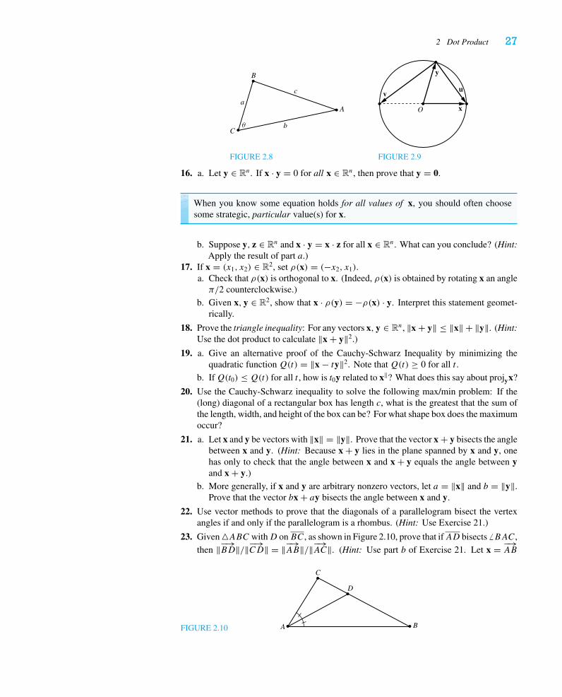
2 Dot Product 27
A
B
C
a
b
c
θ
FIGURE 2.8
x
y
O
uv
FIGURE 2.9
16. a. Let y ∈ Rn. If x · y = 0 for all x ∈ Rn, then prove that y = 0.
When you know some equation holds for all values of x, you should often choosesome strategic, particular value(s) for x.
b. Suppose y, z ∈ Rn and x · y = x · z for all x ∈ Rn. What can you conclude? (Hint:Apply the result of part a.)
17. If x = (x1, x2) ∈ R2, set ρ(x) = (−x2, x1).a. Check that ρ(x) is orthogonal to x. (Indeed, ρ(x) is obtained by rotating x an angleπ/2 counterclockwise.)
b. Given x, y ∈ R2, show that x · ρ(y) = −ρ(x) · y. Interpret this statement geomet-rically.
18. Prove the triangle inequality: For any vectors x, y ∈ Rn, ‖x + y‖ ≤ ‖x‖ + ‖y‖. (Hint:Use the dot product to calculate ‖x + y‖2.)
19. a. Give an alternative proof of the Cauchy-Schwarz Inequality by minimizing thequadratic functionQ(t) = ‖x − ty‖2. Note thatQ(t) ≥ 0 for all t .
b. IfQ(t0) ≤ Q(t) for all t , how is t0y related to x‖? What does this say about projyx?
20. Use the Cauchy-Schwarz inequality to solve the following max/min problem: If the(long) diagonal of a rectangular box has length c, what is the greatest that the sum ofthe length, width, and height of the box can be? For what shape box does the maximumoccur?
21. a. Let x and y be vectors with ‖x‖ = ‖y‖. Prove that the vector x + y bisects the anglebetween x and y. (Hint: Because x + y lies in the plane spanned by x and y, onehas only to check that the angle between x and x + y equals the angle between yand x + y.)
b. More generally, if x and y are arbitrary nonzero vectors, let a = ‖x‖ and b = ‖y‖.Prove that the vector bx + ay bisects the angle between x and y.
22. Use vector methods to prove that the diagonals of a parallelogram bisect the vertexangles if and only if the parallelogram is a rhombus. (Hint: Use Exercise 21.)
23. Given �ABC withD onBC, as shown in Figure 2.10, prove that ifAD bisects � BAC,then ‖−→BD‖/‖−→CD‖ = ‖−→AB‖/‖−→AC‖. (Hint: Use part b of Exercise 21. Let x = −→
AB
FIGURE 2.10 A B
C
D
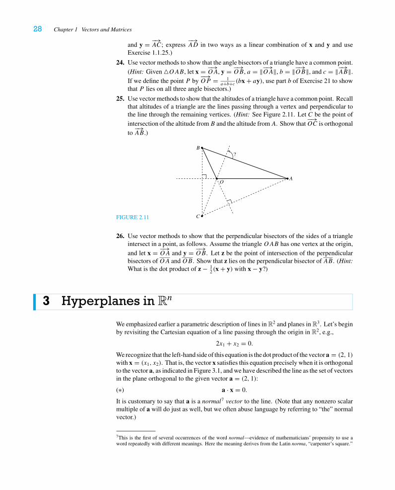
28 Chapter 1 Vectors and Matrices
and y = −→AC; express
−→AD in two ways as a linear combination of x and y and use
Exercise 1.1.25.)
24. Use vector methods to show that the angle bisectors of a triangle have a common point.(Hint: Given �OAB, let x = −→
OA, y = −→OB, a = ‖−→OA‖, b = ‖−→
OB‖, and c = ‖−→AB‖.If we define the point P by
−→OP = 1
a+b+c (bx + ay), use part b of Exercise 21 to showthat P lies on all three angle bisectors.)
25. Use vector methods to show that the altitudes of a triangle have a common point. Recallthat altitudes of a triangle are the lines passing through a vertex and perpendicular tothe line through the remaining vertices. (Hint: See Figure 2.11. Let C be the point ofintersection of the altitude fromB and the altitude fromA. Show that
−→OC is orthogonal
to−→AB.)
FIGURE 2.11
?B
A
C
O
26. Use vector methods to show that the perpendicular bisectors of the sides of a triangleintersect in a point, as follows. Assume the triangleOAB has one vertex at the origin,and let x = −→
OA and y = −→OB. Let z be the point of intersection of the perpendicular
bisectors ofOA andOB. Show that z lies on the perpendicular bisector ofAB. (Hint:What is the dot product of z − 1
2 (x + y) with x − y?)
3 Hyperplanes in Rn
We emphasized earlier a parametric description of lines in R2 and planes in R3. Let’s beginby revisiting the Cartesian equation of a line passing through the origin in R2, e.g.,
2x1 + x2 = 0.
We recognize that the left-hand side of this equation is the dot product of the vector a = (2, 1)with x = (x1, x2). That is, the vector x satisfies this equation precisely when it is orthogonalto the vector a, as indicated in Figure 3.1, and we have described the line as the set of vectorsin the plane orthogonal to the given vector a = (2, 1):
(∗) a · x = 0.
It is customary to say that a is a normal7 vector to the line. (Note that any nonzero scalarmultiple of a will do just as well, but we often abuse language by referring to “the” normalvector.)
7This is the first of several occurrences of the word normal—evidence of mathematicians’ propensity to use aword repeatedly with different meanings. Here the meaning derives from the Latin norma, “carpenter’s square.”
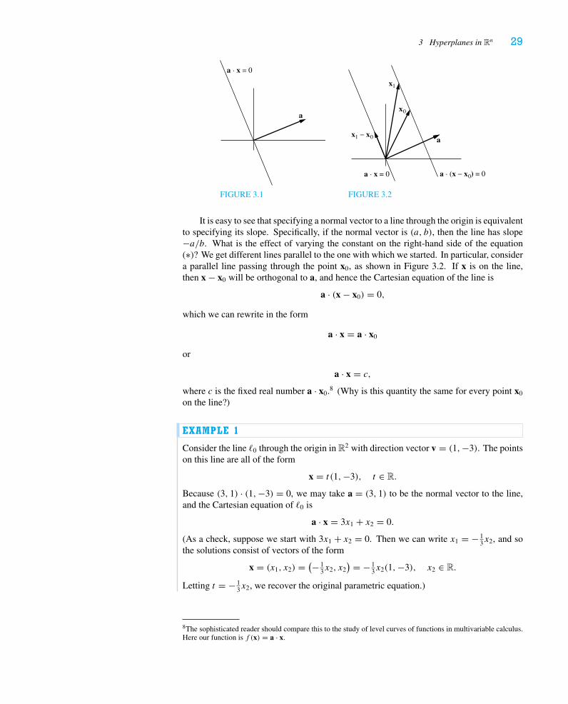
3 Hyperplanes in Rn 29
a
a · x = 0
FIGURE 3.1
a
x1
x1 − x0
a · x = 0 a · (x − x0) = 0
x0
FIGURE 3.2
It is easy to see that specifying a normal vector to a line through the origin is equivalentto specifying its slope. Specifically, if the normal vector is (a, b), then the line has slope−a/b. What is the effect of varying the constant on the right-hand side of the equation(∗)? We get different lines parallel to the one with which we started. In particular, considera parallel line passing through the point x0, as shown in Figure 3.2. If x is on the line,then x − x0 will be orthogonal to a, and hence the Cartesian equation of the line is
a · (x − x0) = 0,
which we can rewrite in the form
a · x = a · x0
or
a · x = c,
where c is the fixed real number a · x0.8 (Why is this quantity the same for every point x0
on the line?)
EXAMPLE 1
Consider the line �0 through the origin in R2 with direction vector v = (1,−3). The pointson this line are all of the form
x = t (1,−3), t ∈ R.
Because (3, 1) · (1,−3) = 0, we may take a = (3, 1) to be the normal vector to the line,and the Cartesian equation of �0 is
a · x = 3x1 + x2 = 0.
(As a check, suppose we start with 3x1 + x2 = 0. Then we can write x1 = − 13x2, and so
the solutions consist of vectors of the form
x = (x1, x2) = (− 13x2, x2
) = − 13x2(1,−3), x2 ∈ R.
Letting t = − 13x2, we recover the original parametric equation.)
8The sophisticated reader should compare this to the study of level curves of functions in multivariable calculus.Here our function is f (x) = a · x.
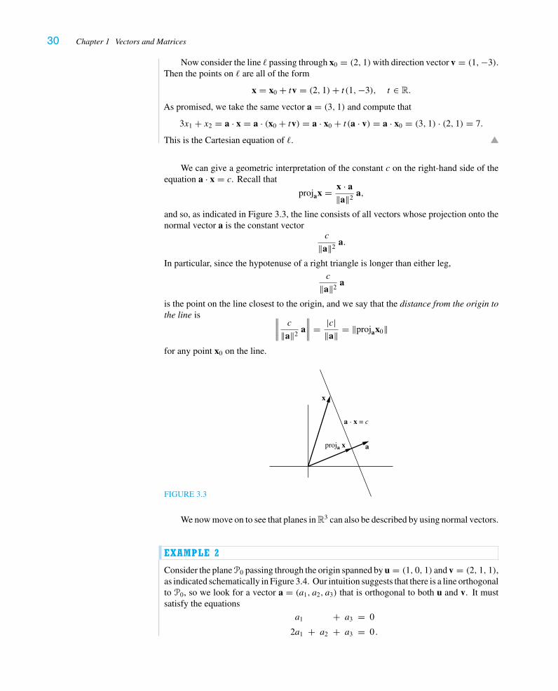
30 Chapter 1 Vectors and Matrices
Now consider the line � passing through x0 = (2, 1)with direction vector v = (1,−3).Then the points on � are all of the form
x = x0 + tv = (2, 1)+ t (1,−3), t ∈ R.
As promised, we take the same vector a = (3, 1) and compute that
3x1 + x2 = a · x = a · (x0 + tv) = a · x0 + t (a · v) = a · x0 = (3, 1) · (2, 1) = 7.
This is the Cartesian equation of �.
We can give a geometric interpretation of the constant c on the right-hand side of theequation a · x = c. Recall that
projax = x · a‖a‖2
a,
and so, as indicated in Figure 3.3, the line consists of all vectors whose projection onto thenormal vector a is the constant vector
c
‖a‖2a.
In particular, since the hypotenuse of a right triangle is longer than either leg,c
‖a‖2a
is the point on the line closest to the origin, and we say that the distance from the origin tothe line is ∥∥∥∥
c
‖a‖2a
∥∥∥∥ = |c|‖a‖ = ‖projax0‖
for any point x0 on the line.
FIGURE 3.3
a
x
proja x
a · x = c
We now move on to see that planes in R3 can also be described by using normal vectors.
EXAMPLE 2
Consider the plane P0 passing through the origin spanned by u = (1, 0, 1) and v = (2, 1, 1),as indicated schematically in Figure 3.4. Our intuition suggests that there is a line orthogonalto P0, so we look for a vector a = (a1, a2, a3) that is orthogonal to both u and v. It mustsatisfy the equations
a1 + a3 = 0
2a1 + a2 + a3 = 0 .
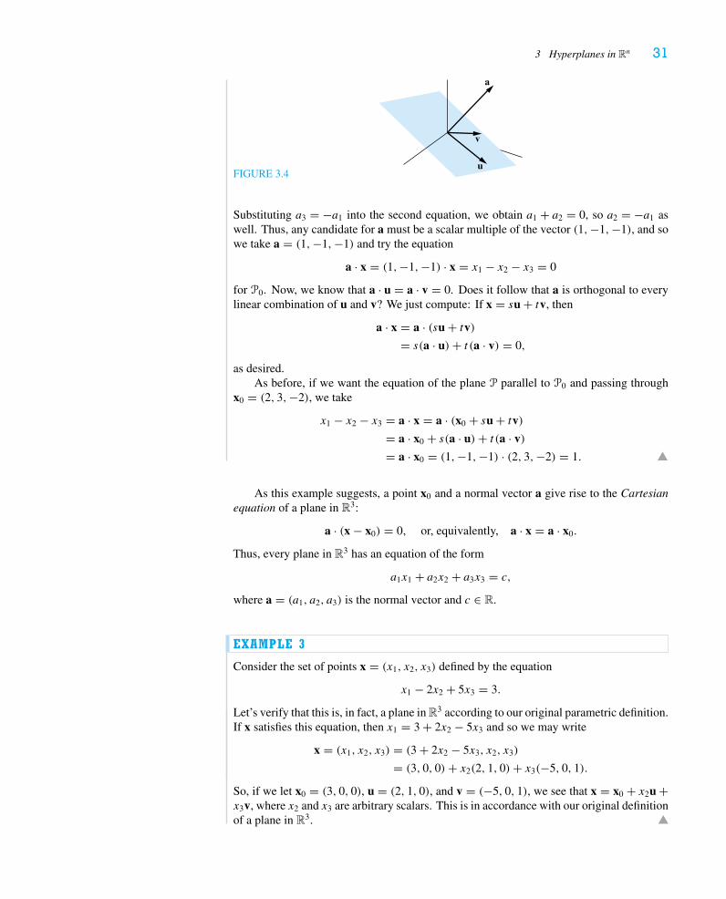
3 Hyperplanes in Rn 31
FIGURE 3.4
a
u
v
Substituting a3 = −a1 into the second equation, we obtain a1 + a2 = 0, so a2 = −a1 aswell. Thus, any candidate for a must be a scalar multiple of the vector (1,−1,−1), and sowe take a = (1,−1,−1) and try the equation
a · x = (1,−1,−1) · x = x1 − x2 − x3 = 0
for P0. Now, we know that a · u = a · v = 0. Does it follow that a is orthogonal to everylinear combination of u and v? We just compute: If x = su + tv, then
a · x = a · (su + tv)= s(a · u)+ t (a · v) = 0,
as desired.As before, if we want the equation of the plane P parallel to P0 and passing through
x0 = (2, 3,−2), we take
x1 − x2 − x3 = a · x = a · (x0 + su + tv)= a · x0 + s(a · u)+ t (a · v)
= a · x0 = (1,−1,−1) · (2, 3,−2) = 1.
As this example suggests, a point x0 and a normal vector a give rise to the Cartesianequation of a plane in R3:
a · (x − x0) = 0, or, equivalently, a · x = a · x0.
Thus, every plane in R3 has an equation of the form
a1x1 + a2x2 + a3x3 = c,
where a = (a1, a2, a3) is the normal vector and c ∈ R.
EXAMPLE 3
Consider the set of points x = (x1, x2, x3) defined by the equation
x1 − 2x2 + 5x3 = 3.
Let’s verify that this is, in fact, a plane in R3 according to our original parametric definition.If x satisfies this equation, then x1 = 3 + 2x2 − 5x3 and so we may write
x = (x1, x2, x3) = (3 + 2x2 − 5x3, x2, x3)
= (3, 0, 0)+ x2(2, 1, 0)+ x3(−5, 0, 1).
So, if we let x0 = (3, 0, 0), u = (2, 1, 0), and v = (−5, 0, 1), we see that x = x0 + x2u +x3v, where x2 and x3 are arbitrary scalars. This is in accordance with our original definitionof a plane in R3.
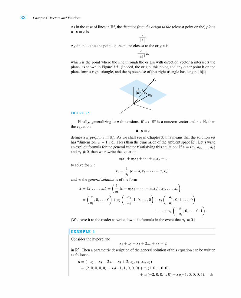
32 Chapter 1 Vectors and Matrices
As in the case of lines in R2, the distance from the origin to the (closest point on the) planea · x = c is |c|
‖a‖ .Again, note that the point on the plane closest to the origin is
c
‖a‖2a,
which is the point where the line through the origin with direction vector a intersects theplane, as shown in Figure 3.5. (Indeed, the origin, this point, and any other point b on theplane form a right triangle, and the hypotenuse of that right triangle has length ‖b‖.)
FIGURE 3.5
a
a
b||a||2
c
Finally, generalizing to n dimensions, if a ∈ Rn is a nonzero vector and c ∈ R, thenthe equation
a · x = c
defines a hyperplane in Rn. As we shall see in Chapter 3, this means that the solution sethas “dimension” n− 1, i.e., 1 less than the dimension of the ambient space Rn. Let’s writean explicit formula for the general vector x satisfying this equation: If a = (a1, a2, . . . , an)
and a1 �= 0, then we rewrite the equation
a1x1 + a2x2 + · · · + anxn = c
to solve for x1:
x1 = 1
a1(c − a2x2 − · · · − anxn) ,
and so the general solution is of the form
x = (x1, . . . , xn) =(
1
a1(c − a2x2 − · · · − anxn) , x2, . . . , xn
)
=(c
a1, 0, . . . , 0
)+ x2
(−a2
a1, 1, 0, . . . , 0
)+ x3
(−a3
a1, 0, 1, . . . , 0
)
+ · · · + xn(
−ana1, 0, . . . , 0, 1
).
(We leave it to the reader to write down the formula in the event that a1 = 0.)
EXAMPLE 4
Consider the hyperplanex1 + x2 − x3 + 2x4 + x5 = 2
in R5. Then a parametric description of the general solution of this equation can be writtenas follows:
x = (−x2 + x3 − 2x4 − x5 + 2, x2, x3, x4, x5)
= (2, 0, 0, 0, 0)+ x2(−1, 1, 0, 0, 0)+ x3(1, 0, 1, 0, 0)
+ x4(−2, 0, 0, 1, 0)+ x5(−1, 0, 0, 0, 1).
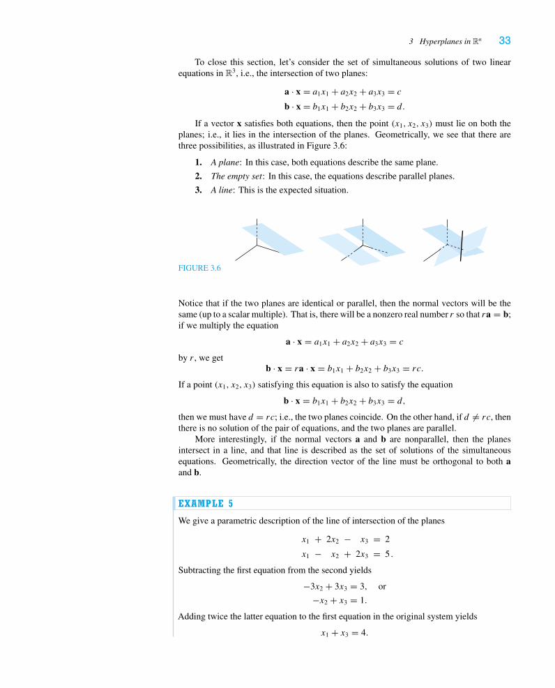
3 Hyperplanes in Rn 33
To close this section, let’s consider the set of simultaneous solutions of two linearequations in R3, i.e., the intersection of two planes:
a · x = a1x1 + a2x2 + a3x3 = cb · x = b1x1 + b2x2 + b3x3 = d.
If a vector x satisfies both equations, then the point (x1, x2, x3) must lie on both theplanes; i.e., it lies in the intersection of the planes. Geometrically, we see that there arethree possibilities, as illustrated in Figure 3.6:
1. A plane: In this case, both equations describe the same plane.
2. The empty set: In this case, the equations describe parallel planes.
3. A line: This is the expected situation.
FIGURE 3.6
Notice that if the two planes are identical or parallel, then the normal vectors will be thesame (up to a scalar multiple). That is, there will be a nonzero real number r so that ra = b;if we multiply the equation
a · x = a1x1 + a2x2 + a3x3 = c
by r , we getb · x = ra · x = b1x1 + b2x2 + b3x3 = rc.
If a point (x1, x2, x3) satisfying this equation is also to satisfy the equation
b · x = b1x1 + b2x2 + b3x3 = d,
then we must have d = rc; i.e., the two planes coincide. On the other hand, if d �= rc, thenthere is no solution of the pair of equations, and the two planes are parallel.
More interestingly, if the normal vectors a and b are nonparallel, then the planesintersect in a line, and that line is described as the set of solutions of the simultaneousequations. Geometrically, the direction vector of the line must be orthogonal to both aand b.
EXAMPLE 5
We give a parametric description of the line of intersection of the planes
x1 + 2x2 − x3 = 2
x1 − x2 + 2x3 = 5 .
Subtracting the first equation from the second yields
−3x2 + 3x3 = 3, or
−x2 + x3 = 1.
Adding twice the latter equation to the first equation in the original system yields
x1 + x3 = 4.
34 Chapter 1 Vectors and Matrices
Thus, we can determine both x1 and x2 in terms of x3:
x1 = 4 − x3
x2 = −1 + x3 .
Then the general solution is of the form
x = (x1, x2, x3) = (4 − x3,−1 + x3, x3) = (4,−1, 0)+ x3(−1, 1, 1).
Indeed, as we mentioned earlier, the direction vector (−1, 1, 1) is orthogonal to a =(1, 2,−1) and b = (1,−1, 2).
Much of the remainder of this course will be devoted to understanding higher-dimen-sional analogues of lines and planes in R3. In particular, we will be concerned with therelation between their parametric description and their description as the set of solutions ofa system of linear equations (geometrically, the intersection of a collection of hyperplanes).The first step toward this goal will be to develop techniques and notation for solving systemsof m linear equations in n variables (as in Example 5, where we solved a system of twolinear equations in three variables). This is the subject of the next section.
Exercises 1.3
1. Give Cartesian equations of the given hyperplanes:a. x = (−1, 2)+ t (3, 2)b.∗ The plane passing through (1, 2, 2) and orthogonal to the line x = (5, 1,−1)+t (−1, 1,−1)
c. The plane passing through (2, 0, 1) and orthogonal to the line x = (2,−1, 3)+t (1, 2,−2)
d.∗ The plane spanned by (1, 1, 1) and (2, 1, 0) and passing through (1, 1, 2)
e. The plane spanned by (1, 0, 1) and (1, 2, 2) and passing through (−1, 1, 1)
f.∗ The hyperplane in R4 through the origin spanned by (1,−1, 1,−1), (1, 1,−1,−1),and (1,−1,−1, 1).
2.∗ Redo Exercise 1.1.12 by finding Cartesian equations of the respective planes.
3. Find the general solution of each of the following equations (presented, as in the text,as a combination of an appropriate number of vectors).a. x1 − 2x2 + 3x3 = 4 (in R3)
b. x1 + x2 − x3 + 2x4 = 0 (in R4)
c.∗ x1 + x2 − x3 + 2x4 = 5 (in R4)
d.∗ x1 − 2x2 + 3x3 = 4 (in R4)
e. x2 + x3 − 3x4 = 2 (in R4)
4. Find a normal vector to the given hyperplane and use it to find the distance from theorigin to the hyperplane.a. x = (−1, 2)+ t (3, 2)b. The plane in R3 given by the equation 2x1 + x2 − x3 = 5
c.∗ The plane passing through (1, 2, 2) and orthogonal to the line x = (3, 1,−1)+t (−1, 1,−1)
d. The plane passing through (2,−1, 1) and orthogonal to the line x = (3, 1, 1)+t (−1, 2, 1)
e.∗ The plane spanned by (1, 1, 4) and (2, 1, 0) and passing through (1, 1, 2)
f. The plane spanned by (1, 1, 1) and (2, 1, 0) and passing through (3, 0, 2)
3 Hyperplanes in Rn 35
g. The hyperplane in R4 spanned by (1,−1, 1,−1), (1, 1,−1,−1), and (1,−1,−1, 1)and passing through (2, 1, 0, 1)
5. Find parametric equations of the line of intersection of the given planes in R3.a. x1 + x2 + x3 = 1, 2x1 + x2 + 2x3 = 1
b. x1 − x2 = 1, x1 + x2 + 2x3 = 5
6.∗ a. Give the general solution of the equation x1 + 5x2 − 2x3 = 0 in R3 (as a linearcombination of two vectors, as in the text).
b. Find a specific solution of the equation x1 + 5x2 − 2x3 = 3 in R3; give the generalsolution.
c. Give the general solution of the equation x1 + 5x2 − 2x3 + x4 = 0 in R4. Now givethe general solution of the equation x1 + 5x2 − 2x3 + x4 = 3.
7.∗ The equation 2x1 − 3x2 = 5 defines a line in R2.a. Give a normal vector a to the line.
b. Find the distance from the origin to the line by using projection.
c. Find the point on the line closest to the origin by using the parametric equation ofthe line through 0 with direction vector a. Double-check your answer to part b.
d. Find the distance from the point w = (3, 1) to the line by using projection.
e. Find the point on the line closest to w by using the parametric equation of the linethrough w with direction vector a. Double-check your answer to part d .
8. The equation 2x1 − 3x2 − 6x3 = −4 defines a plane in R3.a. Give its normal vector a.
b. Find the distance from the origin to the plane by using projection.
c. Find the point on the plane closest to the origin by using the parametric equation ofthe line through 0 with direction vector a. Double-check your answer to part b.
d. Find the distance from the point w = (3,−3,−5) to the plane by using projection.
e. Find the point on the plane closest to w by using the parametric equation of the linethrough w with direction vector a. Double-check your answer to part d .
9. The equation 2x1 + 2x2 − 3x3 + 8x4 = 6 defines a hyperplane in R4.a. Give a normal vector a to the hyperplane.
b. Find the distance from the origin to the hyperplane using projection.
c. Find the point on the hyperplane closest to the origin by using the parametric equationof the line through 0 with direction vector a. Double-check your answer to part b.
d. Find the distance from the point w = (1, 1, 1, 1) to the hyperplane using dot prod-ucts.
e. Find the point on the hyperplane closest to w by using the parametric equation ofthe line through w with direction vector a. Double-check your answer to part d .
10. a.∗ The equations x1 = 0 and x2 = 0 describe planes in R3 that contain the x3-axis.Write down the Cartesian equation of a general such plane.
b. The equations x1 − x2 = 0 and x1 − x3 = 0 describe planes in R3 that contain theline through the origin with direction vector (1, 1, 1). Write down the Cartesianequation of a general such plane.
11. a. Assume b and c are nonparallel vectors in R3. Generalizing the result of Exercise10, show that the plane a · x = 0 contains the intersection of the planes b · x = 0and c · x = 0 if and only if a = sb + tc for some s, t ∈ R, not both 0. Describe thisresult geometrically.
b. Assume b and c are nonparallel vectors in Rn. Formulate a conjecture about whichhyperplanes a · x = 0 in Rn contain the intersection of the hyperplanes b · x = 0and c · x = 0. Prove as much of your conjecture as you can.
36 Chapter 1 Vectors and Matrices
12. Suppose a �= 0 and P ⊂ R3 is the plane through the origin with normal vector a.Suppose P is spanned by u and v.a. Suppose u · v = 0. Show that for every x ∈ P, we have
x = projux + projvx.
b. Suppose u · v = 0. Show that for every x ∈ R3, we have
x = projax + projux + projvx.
(Hint: Apply part a to the vector x − projax.)
c. Give an example to show the result of part a is false when u and v are not orthogonal.
13. Consider the line � in R3 given parametrically by x = x0 + ta. Let P0 denote the planethrough the origin with normal vector a (so it is orthogonal to �).a. Show that � and P0 intersect in the point x0 − projax0.
b. Conclude that the distance from the origin to � is ‖x0 − projax0‖.
4 Systems of Linear Equations and GaussianElimination
In this section we give an explicit algorithm for solving a system ofm linear equationsin n variables. Unfortunately, this is a little bit like giving the technical description of tyinga shoe—it is much easier to do it than to read how to do it. For that reason, before embarkingon the technicalities of the process, we will present here a few examples and introduce thenotation of matrices. On the other hand, once the technique is mastered, it will be importantfor us to understand why it yields all solutions of the system of equations. For this reason,it is is essential to understand Theorem 4.1.
To begin with, a linear equation in the n variables x1, x2, . . . , xn is an equation of theform
a1x1 + a2x2 + · · · + anxn = b,
where the coefficients ai , i = 1, . . . , n, are fixed real numbers and b is a fixed real number.Notice that if we let a = (a1, . . . , an) and x = (x1, . . . , xn), then we can write this equationin vector notation as
a · x = b.
We recognize this as the equation of a hyperplane in Rn, and a vector x solves the equationprecisely when the point x lies on that hyperplane.
A system of m linear equations in n variables consists of m such equations:
a11x1 + a12x2 + · · · + a1nxn = b1
a21x1 + a22x2 + · · · + a2nxn = b2
...
am1x1 + am2x2 + · · · + amnxn = bm.
The notation appears cumbersome, but we have to live with it. A pair of subscripts is neededon the coefficient aij to indicate in which equation it appears (the first index, i) and to which
4 Systems of Linear Equations and Gaussian Elimination 37
variable it is associated (the second index, j ). A solution x = (x1, . . . , xn) is an n-tupleof real numbers that satisfies all m of the equations. Thus, a solution gives a point in theintersection of the m hyperplanes.
To solve a system of linear equations, we want to give a complete parametric descriptionof the solutions, as we did for hyperplanes and for the intersection of two planes in Example 5in the preceding section. We will call this the general solution of the system. Some systemsare relatively simple to solve. For example, the system
x1 = 1
x2 = 2
x3 = −1
has exactly one solution, namely x = (1, 2,−1). This is the only point common to the threeplanes described by the three equations. A slightly more complicated example is
x1 − x3 = 1
x2 + 2x3 = 2 .
These equations enable us to determine x1 and x2 in terms of x3; in particular, we can writex1 = 1 + x3 and x2 = 2 − 2x3, where x3 is free to take on any real value. Thus, any solutionof this system is of the form
x = (1 + t, 2 − 2t, t) = (1, 2, 0)+ t (1,−2, 1) for some t ∈ R.
It is easily checked that every vector of this form is in fact a solution, as (1 + t)− t = 1and (2 − 2t)+ 2t = 2 for every t ∈ R. Thus, we see that the intersection of the two givenplanes is the line in R3 passing through (1, 2, 0) with direction vector (1,−2, 1).
One should note that in the preceding example, we chose to solve for x1 and x2 in termsof x3. We could just as well have solved, say, for x2 and x3 in terms of x1 by first writingx3 = x1 − 1 and then substituting to obtain x2 = 4 − 2x1. Then we would end up writing
x = (s, 4 − 2s,−1 + s) = (0, 4,−1)+ s(1,−2, 1) for some s ∈ R.
We will soon give an algorithm for solving systems of linear equations that will eliminatethe ambiguity in deciding which variables should be taken as parameters. The variablesthat are allowed to vary freely (as parameters) are called free variables, and the remainingvariables, which can be expressed in terms of the free variables, are called pivot variables.Broadly speaking, if there are m equations, whenever possible we will try to solve for thefirst m variables (assuming there are that many) in terms of the remaining variables. Thisis not always possible (for example, the first variable may not even appear in any of theequations), so we will need to specify a general procedure to select which will be pivotvariables and which will be free.
When we are solving a system of equations, there are three basic algebraic operationswe can perform that will not affect the solution set. They are the following elementaryoperations:
(i) Interchange any pair of equations.
(ii) Multiply any equation by a nonzero real number.
(iii) Replace any equation by its sum with a multiple of any other equation.
The first two are probably so obvious that it seems silly to write them down; however, soonyou will see their importance. It is not obvious that the third operation does not changethe solution set; we will address this in Theorem 4.1. First, let’s consider an example ofsolving a system of linear equations using these operations.
38 Chapter 1 Vectors and Matrices
EXAMPLE 1
Consider the system of linear equations
3x1 − 2x2 + 2x3 + 9x4 = 4
2x1 + 2x2 − 2x3 − 4x4 = 6 .
We can use operation (i) to replace this system with
2x1 + 2x2 − 2x3 − 4x4 = 6
3x1 − 2x2 + 2x3 + 9x4 = 4;then we use operation (ii), multiplying the first equation by 1/2, to get
x1 + x2 − x3 − 2x4 = 3
3x1 − 2x2 + 2x3 + 9x4 = 4;now we use operation (iii), adding −3 times the first equation to the second:
x1 + x2 − x3 − 2x4 = 3
− 5x2 + 5x3 + 15x4 = −5 .
Next we use operation (ii) again, multiplying the second equation by −1/5, to obtain
x1 + x2 − x3 − 2x4 = 3
x2 − x3 − 3x4 = 1;finally, we use operation (iii), adding −1 times the second equation to the first:
x1 + x4 = 2
x2 − x3 − 3x4 = 1 .
From this we see that x1 and x2 are determined by x3 and x4, both of which are free to takeon any values. Thus, we read off the general solution of the system of equations:
x1 = 2 − x4
x2 = 1 + x3 + 3x4
x3 = x3
x4 = x4
In vector form, the general solution is
x = (x1, x2, x3, x4) = (2, 1, 0, 0)+ x3(0, 1, 1, 0)+ x4(−1, 3, 0, 1),
which is the parametric representation of a plane in R4.
Before describing the algorithm for solving a general system of linear equations, wewant to introduce some notation to make the calculations less cumbersome to write out.We begin with a system of m equations in n unknowns:
a11x1 + a12x2 + · · · + a1nxn = b1
a21x1 + a22x2 + · · · + a2nxn = b2
...
am1x1 + am2x2 + · · · + amnxn = bm.
4 Systems of Linear Equations and Gaussian Elimination 39
We can simplify our notation somewhat by writing the equations in vector notation:
A1 · x = b1
A2 · x = b2
...
Am · x = bm,
where Ai = (ai1, ai2, . . . , ain) ∈ Rn, i = 1, 2, . . . , m. To simplify the notation further, weintroduce the m× n (read “m by n”) matrix9
A =
⎡⎢⎢⎢⎢⎢⎣
a11 . . . a1n
a21 . . . a2n
.... . .
...
am1 . . . amn
⎤⎥⎥⎥⎥⎥⎦
and the column vectors10
x =
⎡⎢⎢⎢⎢⎢⎣
x1
x2
...
xn
⎤⎥⎥⎥⎥⎥⎦
∈ Rn and b =
⎡⎢⎢⎢⎢⎢⎣
b1
b2
...
bm
⎤⎥⎥⎥⎥⎥⎦
∈ Rm,
and write our equations asAx = b,
where the multiplication on the left-hand side is defined to be
Ax =
⎡⎢⎢⎢⎢⎢⎣
A1 · x
A2 · x...
Am · x
⎤⎥⎥⎥⎥⎥⎦
=
⎡⎢⎢⎢⎢⎢⎣
a11x1 + · · · + a1nxn
a21x1 + · · · + a2nxn...
am1x1 + · · · + amnxn
⎤⎥⎥⎥⎥⎥⎦.
We will discuss the algebraic and geometric properties of matrices a bit later, but for now wesimply use them as convenient shorthand notation for systems of equations. We emphasizethat an m× n matrix has m rows and n columns. The coefficient aij appearing in the i th
row and the j th column is called the ij -entry of A. We say that two matrices are equal ifthey have the same shape (that is, if they have equal numbers of rows and equal numbers ofcolumns) and their corresponding entries are equal. As we did above, we will customarilydenote the row vectors of the matrix A by A1, . . . ,Am ∈ Rn.
We reiterate that a solution x of the system of equations Ax = b is a vector having therequisite dot products with the row vectors Ai :
Ai · x = bi for all i = 1, 2, . . . , m.
That is, the system of equations describes the intersection of them hyperplanes with normalvectors Ai and at (signed) distance bi/‖Ai‖ from the origin. To give the general solution,we must find a parametric representation of this intersection.
9The word matrix derives from the Latin matrix, “womb” (originally, “pregnant animal”), from mater, “mother.”
10We shall henceforth try to write vectors as columns, unless doing so might cause undue typographical hardship.

40 Chapter 1 Vectors and Matrices
Notice that the first two types of elementary operations do not change this collectionof hyperplanes, so it is no surprise that these operations do not affect the solution setof the system of equations. On the other hand, the third type actually changes one of thehyperplanes without changing the intersection. To see why, suppose a and b are nonparalleland consider the pairs of equations
a · x = 0 (a + cb) · x = 0and
b · x = 0 b · x = 0.
Suppose x satisfies the first set of equations, so a · x = 0 and b · x = 0; then x satisfiesthe second set as well, since (a + cb) · x = (a · x)+ c(b · x) = 0 + c0 = 0 and b · x = 0remains true. Conversely, if x satisfies the second set of equations, we have b · x = 0and a · x = (a + cb) · x − c(b · x) = 0 − c0 = 0, so x also satisfies the first set. Thus thesolution sets are identical. Geometrically, as shown in Figure 4.1, taking a bit of poeticlicense, we can think of the hyperplanes a · x = 0 and b · x = 0 as the covers of a book,and the solutions x will form the “spine” of the book. The typical equation (a + cb) · x = 0describes one of the pages of the book, and that page intersects either of the covers preciselyin the same spine. This follows from the fact that the spine consists of all vectors orthogonalto the plane spanned by a and b; this is identical to the plane spanned by a + cb and b(or a).
FIGURE 4.1
a · x = 0
b · x = 0
(a + cb) · x = 0
a + cb
b a
The general result is the following:
Theorem 4.1. If a system of equations Ax = b is changed into the new system Cx = d byelementary operations, then the systems have the same set of solutions.
Proof. We need to show that every solution of Ax = b is also a solution of Cx = d, andvice versa. Start with a solution u of Ax = b. Denoting the rows of A by A1, . . . ,Am, wehave
A1 · u = b1
A2 · u = b2
...
Am · u = bm
If we apply an elementary operation of type (i), u still satisfies precisely the same list ofequations. If we apply an elementary operation of type (ii), say multiplying the kth equationby r �= 0, we note that if u satisfies Ak · u = bk , then it must satisfy (rAk) · u = rbk . As
4 Systems of Linear Equations and Gaussian Elimination 41
for an elementary operation of type (iii), suppose we add r times the kth equation to the �th;since Ak · u = bk and A� · u = b�, it follows that
(rAk + A�) · u = (rAk · u)+ (A� · u) = rbk + b�,and so u satisfies the “new” �th equation.
To prove conversely that if u satisfiesCx = d, then it satisfiesAx = b, we merely notethat each argument we’ve given can be reversed; in particular, the inverse of an elementaryoperation is again an elementary operation. Note that it is important here that r �= 0 foran operation of type (ii).
We introduce one further piece of shorthand notation, the augmented matrix
[A | b ] =
⎡⎢⎢⎢⎢⎢⎣
a11 . . . a1n b1
a21 . . . a2n b2
.... . .
......
am1 . . . amn bm
⎤⎥⎥⎥⎥⎥⎦.
Notice that the augmented matrix contains all of the information of the original system ofequations, because we can recover the latter by filling in the xi’s, +’s, and =’s as needed.
The elementary operations on a system of equations become operations on the rows ofthe augmented matrix; in this setting, we refer to them as elementary row operations of thecorresponding three types:
(i) Interchange any pair of rows.
(ii) Multiply all the entries of any row by a nonzero real number.
(iii) Replace any row by its sum with a multiple of any other row.
Since we have established that elementary operations do not affect the solution set of asystem of equations, we can freely perform elementary row operations on the augmentedmatrix of a system of equations with the goal of finding an “equivalent” augmented matrixfrom which we can easily read off the general solution.
EXAMPLE 2
We revisit Example 1 in the notation of augmented matrices. To solve
3x1 − 2x2 + 2x3 + 9x4 = 4
2x1 + 2x2 − 2x3 − 4x4 = 6 ,
we begin by forming the appropriate augmented matrix[
3 −2 2 9 4
2 2 −2 −4 6
].
We denote the process of performing row operations by the symbol � and (in this example)we indicate above it the type of operation we are performing:[
3 −2 2 9 4
2 2 −2 −4 6
](i)�[
2 2 −2 −4 6
3 −2 2 9 4
](ii)�[
1 1 −1 −2 3
3 −2 2 9 4
]
(iii)�[
1 1 −1 −2 3
0 −5 5 15 −5
](ii)�[
1 1 −1 −2 3
0 1 −1 −3 1
](iii)�[
1 0 0 1 2
0 1 −1 −3 1
].
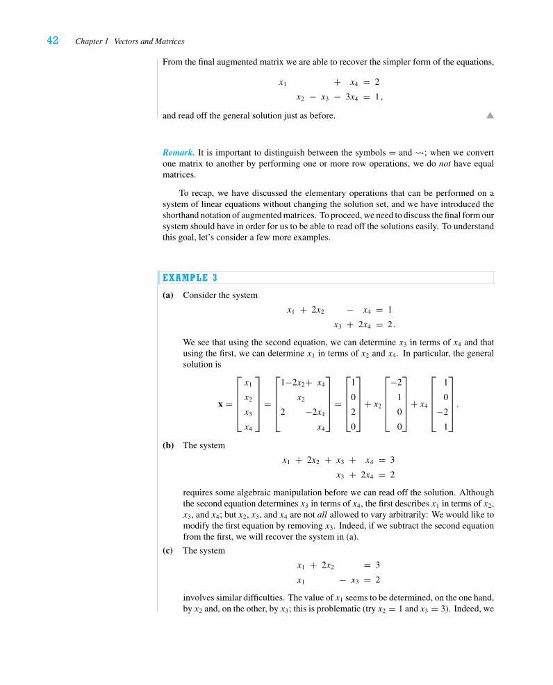
42 Chapter 1 Vectors and Matrices
From the final augmented matrix we are able to recover the simpler form of the equations,
x1 + x4 = 2
x2 − x3 − 3x4 = 1 ,
and read off the general solution just as before.
Remark. It is important to distinguish between the symbols = and �; when we convertone matrix to another by performing one or more row operations, we do not have equalmatrices.
To recap, we have discussed the elementary operations that can be performed on asystem of linear equations without changing the solution set, and we have introduced theshorthand notation of augmented matrices. To proceed, we need to discuss the final form oursystem should have in order for us to be able to read off the solutions easily. To understandthis goal, let’s consider a few more examples.
EXAMPLE 3
(a) Consider the system
x1 + 2x2 − x4 = 1
x3 + 2x4 = 2 .
We see that using the second equation, we can determine x3 in terms of x4 and thatusing the first, we can determine x1 in terms of x2 and x4. In particular, the generalsolution is
x =
⎡⎢⎢⎢⎢⎣
x1
x2
x3
x4
⎤⎥⎥⎥⎥⎦
=
⎡⎢⎢⎢⎢⎣
1−2x2+ x4
x2
2 −2x4
x4
⎤⎥⎥⎥⎥⎦
=
⎡⎢⎢⎢⎢⎣
1
0
2
0
⎤⎥⎥⎥⎥⎦
+ x2
⎡⎢⎢⎢⎢⎣
−2
1
0
0
⎤⎥⎥⎥⎥⎦
+ x4
⎡⎢⎢⎢⎢⎣
1
0
−2
1
⎤⎥⎥⎥⎥⎦.
(b) The system
x1 + 2x2 + x3 + x4 = 3
x3 + 2x4 = 2
requires some algebraic manipulation before we can read off the solution. Althoughthe second equation determines x3 in terms of x4, the first describes x1 in terms of x2,x3, and x4; but x2, x3, and x4 are not all allowed to vary arbitrarily: We would like tomodify the first equation by removing x3. Indeed, if we subtract the second equationfrom the first, we will recover the system in (a).
(c) The system
x1 + 2x2 = 3
x1 − x3 = 2
involves similar difficulties. The value of x1 seems to be determined, on the one hand,by x2 and, on the other, by x3; this is problematic (try x2 = 1 and x3 = 3). Indeed, we
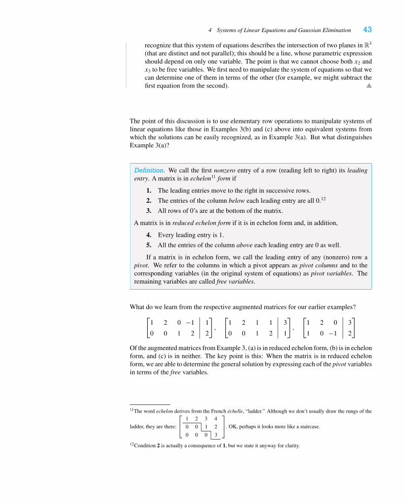
4 Systems of Linear Equations and Gaussian Elimination 43
recognize that this system of equations describes the intersection of two planes in R3
(that are distinct and not parallel); this should be a line, whose parametric expressionshould depend on only one variable. The point is that we cannot choose both x2 andx3 to be free variables. We first need to manipulate the system of equations so that wecan determine one of them in terms of the other (for example, we might subtract thefirst equation from the second).
The point of this discussion is to use elementary row operations to manipulate systems oflinear equations like those in Examples 3(b) and (c) above into equivalent systems fromwhich the solutions can be easily recognized, as in Example 3(a). But what distinguishesExample 3(a)?
Definition. We call the first nonzero entry of a row (reading left to right) its leadingentry. A matrix is in echelon11 form if
1. The leading entries move to the right in successive rows.
2. The entries of the column below each leading entry are all 0.12
3. All rows of 0’s are at the bottom of the matrix.
A matrix is in reduced echelon form if it is in echelon form and, in addition,
4. Every leading entry is 1.
5. All the entries of the column above each leading entry are 0 as well.
If a matrix is in echelon form, we call the leading entry of any (nonzero) row apivot. We refer to the columns in which a pivot appears as pivot columns and to thecorresponding variables (in the original system of equations) as pivot variables. Theremaining variables are called free variables.
What do we learn from the respective augmented matrices for our earlier examples?[
1 2 0 −1 1
0 0 1 2 2
],
[1 2 1 1 3
0 0 1 2 1
],
[1 2 0 3
1 0 −1 2
]
Of the augmented matrices from Example 3, (a) is in reduced echelon form, (b) is in echelonform, and (c) is in neither. The key point is this: When the matrix is in reduced echelonform, we are able to determine the general solution by expressing each of the pivot variablesin terms of the free variables.
11The word echelon derives from the French échelle, “ladder.” Although we don’t usually draw the rungs of the
ladder, they are there:
⎡⎢⎣
1 2 3 4
0 0 1 2
0 0 0 3
⎤⎥⎦. OK, perhaps it looks more like a staircase.
12Condition 2 is actually a consequence of 1, but we state it anyway for clarity.
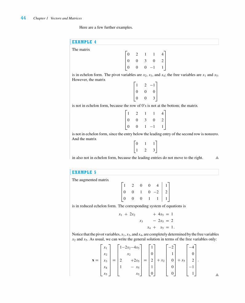
44 Chapter 1 Vectors and Matrices
Here are a few further examples.
EXAMPLE 4
The matrix ⎡⎢⎢⎣
0 2 1 1 4
0 0 3 0 2
0 0 0 −1 1
⎤⎥⎥⎦
is in echelon form. The pivot variables are x2, x3, and x4; the free variables are x1 and x5.However, the matrix ⎡
⎢⎢⎣1 2 −1
0 0 0
0 0 3
⎤⎥⎥⎦
is not in echelon form, because the row of 0’s is not at the bottom; the matrix⎡⎢⎢⎣
1 2 1 1 4
0 0 3 0 2
0 0 1 −1 1
⎤⎥⎥⎦
is not in echelon form, since the entry below the leading entry of the second row is nonzero.And the matrix [
0 1 1
1 2 3
]
in also not in echelon form, because the leading entries do not move to the right.
EXAMPLE 5
The augmented matrix ⎡⎢⎢⎣
1 2 0 0 4 1
0 0 1 0 −2 2
0 0 0 1 1 1
⎤⎥⎥⎦
is in reduced echelon form. The corresponding system of equations is
x1 + 2x2 + 4x5 = 1
x3 − 2x5 = 2
x4 + x5 = 1 .
Notice that the pivot variables, x1, x3, andx4, are completely determined by the free variablesx2 and x5. As usual, we can write the general solution in terms of the free variables only:
x =
⎡⎢⎢⎢⎢⎢⎢⎢⎣
x1
x2
x3
x4
x5
⎤⎥⎥⎥⎥⎥⎥⎥⎦
=
⎡⎢⎢⎢⎢⎢⎢⎢⎣
1−2x2−4x5
x2
2 +2x5
1 − x5
x5
⎤⎥⎥⎥⎥⎥⎥⎥⎦
=
⎡⎢⎢⎢⎢⎢⎢⎢⎣
1
0
2
1
0
⎤⎥⎥⎥⎥⎥⎥⎥⎦
+ x2
⎡⎢⎢⎢⎢⎢⎢⎢⎣
−2
1
0
0
0
⎤⎥⎥⎥⎥⎥⎥⎥⎦
+ x5
⎡⎢⎢⎢⎢⎢⎢⎢⎣
−4
0
2
−1
1
⎤⎥⎥⎥⎥⎥⎥⎥⎦.
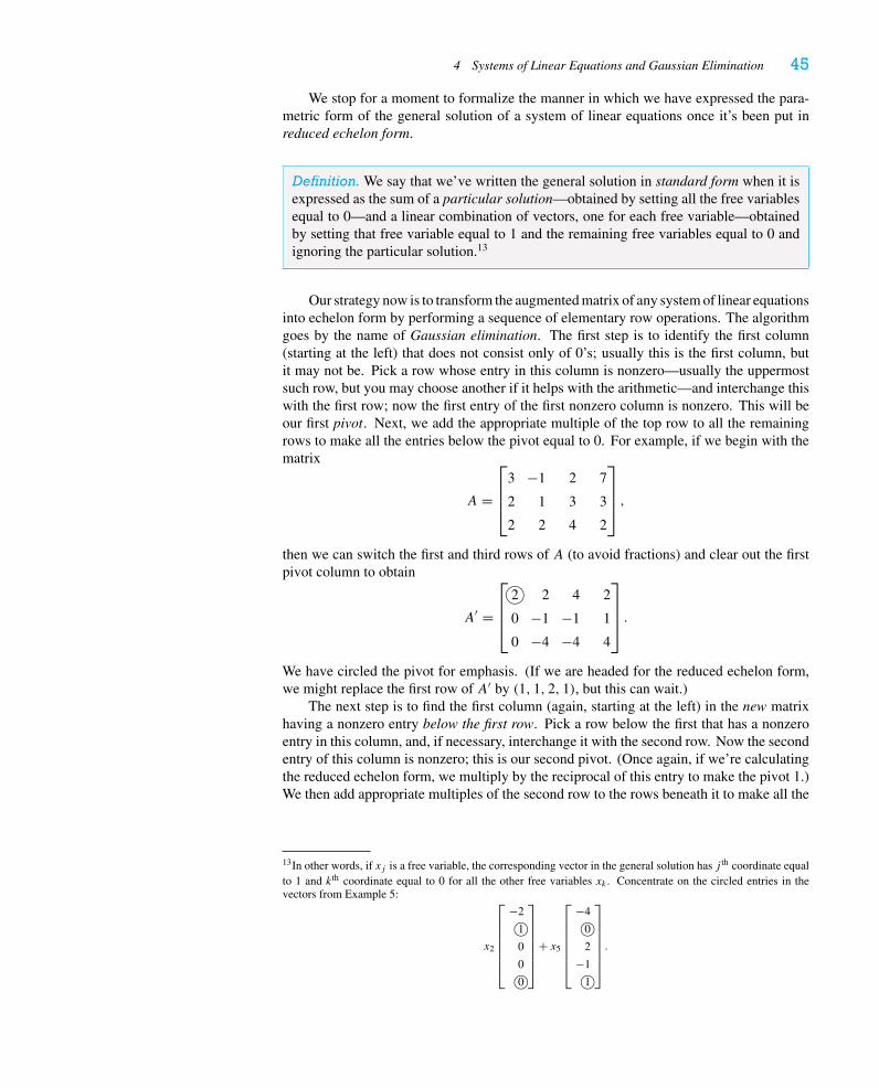
4 Systems of Linear Equations and Gaussian Elimination 45
We stop for a moment to formalize the manner in which we have expressed the para-metric form of the general solution of a system of linear equations once it’s been put inreduced echelon form.
Definition. We say that we’ve written the general solution in standard form when it isexpressed as the sum of a particular solution—obtained by setting all the free variablesequal to 0—and a linear combination of vectors, one for each free variable—obtainedby setting that free variable equal to 1 and the remaining free variables equal to 0 andignoring the particular solution.13
Our strategy now is to transform the augmented matrix of any system of linear equationsinto echelon form by performing a sequence of elementary row operations. The algorithmgoes by the name of Gaussian elimination. The first step is to identify the first column(starting at the left) that does not consist only of 0’s; usually this is the first column, butit may not be. Pick a row whose entry in this column is nonzero—usually the uppermostsuch row, but you may choose another if it helps with the arithmetic—and interchange thiswith the first row; now the first entry of the first nonzero column is nonzero. This will beour first pivot. Next, we add the appropriate multiple of the top row to all the remainingrows to make all the entries below the pivot equal to 0. For example, if we begin with thematrix
A =
⎡⎢⎢⎣
3 −1 2 7
2 1 3 3
2 2 4 2
⎤⎥⎥⎦ ,
then we can switch the first and third rows of A (to avoid fractions) and clear out the firstpivot column to obtain
A′ =
⎡⎢⎢⎣
�2 2 4 2
0 −1 −1 1
0 −4 −4 4
⎤⎥⎥⎦ .
We have circled the pivot for emphasis. (If we are headed for the reduced echelon form,we might replace the first row of A′ by (1, 1, 2, 1), but this can wait.)
The next step is to find the first column (again, starting at the left) in the new matrixhaving a nonzero entry below the first row. Pick a row below the first that has a nonzeroentry in this column, and, if necessary, interchange it with the second row. Now the secondentry of this column is nonzero; this is our second pivot. (Once again, if we’re calculatingthe reduced echelon form, we multiply by the reciprocal of this entry to make the pivot 1.)We then add appropriate multiples of the second row to the rows beneath it to make all the
13In other words, if xj is a free variable, the corresponding vector in the general solution has j th coordinate equalto 1 and kth coordinate equal to 0 for all the other free variables xk . Concentrate on the circled entries in thevectors from Example 5:
x2
⎡⎢⎢⎢⎢⎢⎢⎣
−2�10
0�0
⎤⎥⎥⎥⎥⎥⎥⎦
+ x5
⎡⎢⎢⎢⎢⎢⎢⎣
−4�0
2
−1�1
⎤⎥⎥⎥⎥⎥⎥⎦.
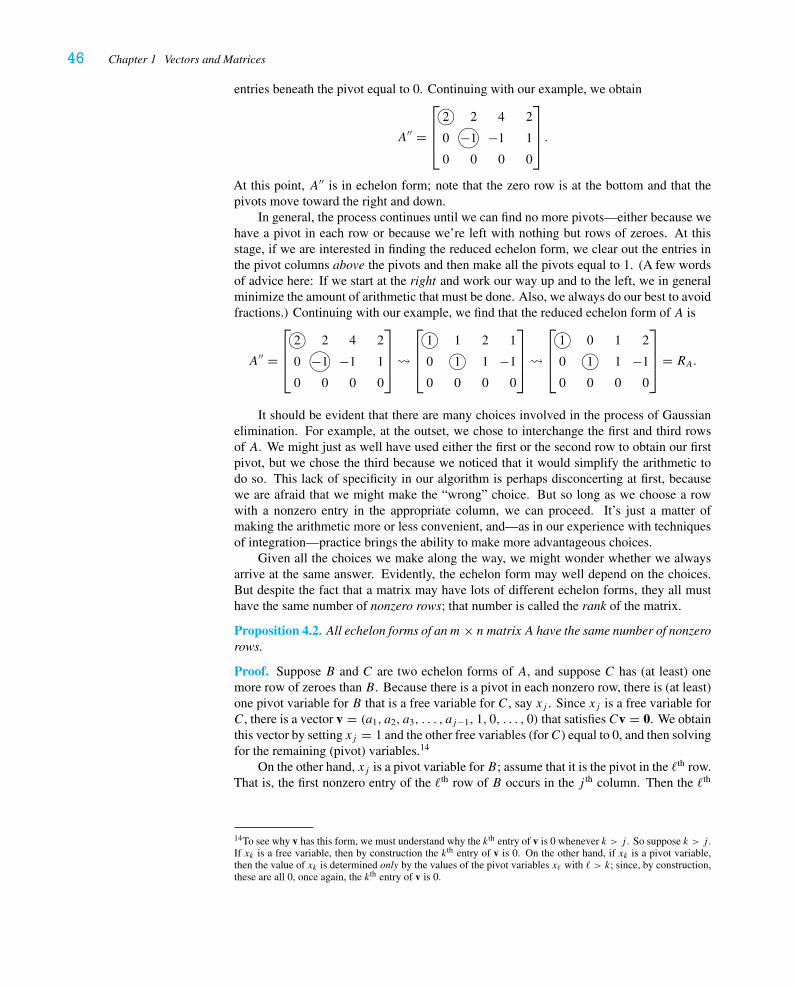
46 Chapter 1 Vectors and Matrices
entries beneath the pivot equal to 0. Continuing with our example, we obtain
A′′ =
⎡⎢⎢⎣
�2 2 4 2
0 �−1 −1 1
0 0 0 0
⎤⎥⎥⎦ .
At this point, A′′ is in echelon form; note that the zero row is at the bottom and that thepivots move toward the right and down.
In general, the process continues until we can find no more pivots—either because wehave a pivot in each row or because we’re left with nothing but rows of zeroes. At thisstage, if we are interested in finding the reduced echelon form, we clear out the entries inthe pivot columns above the pivots and then make all the pivots equal to 1. (A few wordsof advice here: If we start at the right and work our way up and to the left, we in generalminimize the amount of arithmetic that must be done. Also, we always do our best to avoidfractions.) Continuing with our example, we find that the reduced echelon form of A is
A′′ =
⎡⎢⎢⎣
�2 2 4 2
0 �−1 −1 1
0 0 0 0
⎤⎥⎥⎦�
⎡⎢⎢⎣
�1 1 2 1
0 �1 1 −1
0 0 0 0
⎤⎥⎥⎦ �
⎡⎢⎢⎣
�1 0 1 2
0 �1 1 −1
0 0 0 0
⎤⎥⎥⎦ = RA.
It should be evident that there are many choices involved in the process of Gaussianelimination. For example, at the outset, we chose to interchange the first and third rowsof A. We might just as well have used either the first or the second row to obtain our firstpivot, but we chose the third because we noticed that it would simplify the arithmetic todo so. This lack of specificity in our algorithm is perhaps disconcerting at first, becausewe are afraid that we might make the “wrong” choice. But so long as we choose a rowwith a nonzero entry in the appropriate column, we can proceed. It’s just a matter ofmaking the arithmetic more or less convenient, and—as in our experience with techniquesof integration—practice brings the ability to make more advantageous choices.
Given all the choices we make along the way, we might wonder whether we alwaysarrive at the same answer. Evidently, the echelon form may well depend on the choices.But despite the fact that a matrix may have lots of different echelon forms, they all musthave the same number of nonzero rows; that number is called the rank of the matrix.
Proposition 4.2. All echelon forms of anm× nmatrixA have the same number of nonzerorows.
Proof. Suppose B and C are two echelon forms of A, and suppose C has (at least) onemore row of zeroes than B. Because there is a pivot in each nonzero row, there is (at least)one pivot variable for B that is a free variable for C, say xj . Since xj is a free variable forC, there is a vector v = (a1, a2, a3, . . . , aj−1, 1, 0, . . . , 0) that satisfies Cv = 0. We obtainthis vector by setting xj = 1 and the other free variables (forC) equal to 0, and then solvingfor the remaining (pivot) variables.14
On the other hand, xj is a pivot variable for B; assume that it is the pivot in the �th row.That is, the first nonzero entry of the �th row of B occurs in the j th column. Then the �th
14To see why v has this form, we must understand why the kth entry of v is 0 whenever k > j . So suppose k > j .If xk is a free variable, then by construction the kth entry of v is 0. On the other hand, if xk is a pivot variable,then the value of xk is determined only by the values of the pivot variables x� with � > k; since, by construction,these are all 0, once again, the kth entry of v is 0.
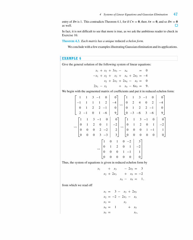
4 Systems of Linear Equations and Gaussian Elimination 47
entry of Bv is 1. This contradicts Theorem 4.1, for if Cv = 0, thenAv = 0, and so Bv = 0as well.
In fact, it is not difficult to see that more is true, as we ask the ambitious reader to check inExercise 16:
Theorem 4.3. Each matrix has a unique reduced echelon form.
We conclude with a few examples illustrating Gaussian elimination and its applications.
EXAMPLE 6
Give the general solution of the following system of linear equations:
x1 + x2 + 3x3 − x4 = 0
−x1 + x2 + x3 + x4 + 2x5 = −4
x2 + 2x3 + 2x4 − x5 = 0
2x1 − x2 + x4 − 6x5 = 9 .
We begin with the augmented matrix of coefficients and put it in reduced echelon form:⎡⎢⎢⎢⎢⎣
1 1 3 −1 0 0
−1 1 1 1 2 −4
0 1 2 2 −1 0
2 −1 0 1 −6 9
⎤⎥⎥⎥⎥⎦
�
⎡⎢⎢⎢⎢⎣
1 1 3 −1 0 0
0 2 4 0 2 −4
0 1 2 2 −1 0
0 −3 −6 3 −6 9
⎤⎥⎥⎥⎥⎦
�
⎡⎢⎢⎢⎢⎣
1 1 3 −1 0 0
0 1 2 0 1 −2
0 0 0 2 −2 2
0 0 0 3 −3 3
⎤⎥⎥⎥⎥⎦
�
⎡⎢⎢⎢⎢⎣
1 1 3 −1 0 0
0 1 2 0 1 −2
0 0 0 1 −1 1
0 0 0 0 0 0
⎤⎥⎥⎥⎥⎦
�
⎡⎢⎢⎢⎢⎣
1 0 1 0 −2 3
0 1 2 0 1 −2
0 0 0 1 −1 1
0 0 0 0 0 0
⎤⎥⎥⎥⎥⎦
Thus, the system of equations is given in reduced echelon form by
x1 + x3 − 2x5 = 3
x2 + 2x3 + x5 = −2
x4 − x5 = 1 ,
from which we read off
x1 = 3 − x3 + 2x5
x2 = −2 − 2x3 − x5
x3 = x3
x4 = 1 + x5
x5 = x5 ,
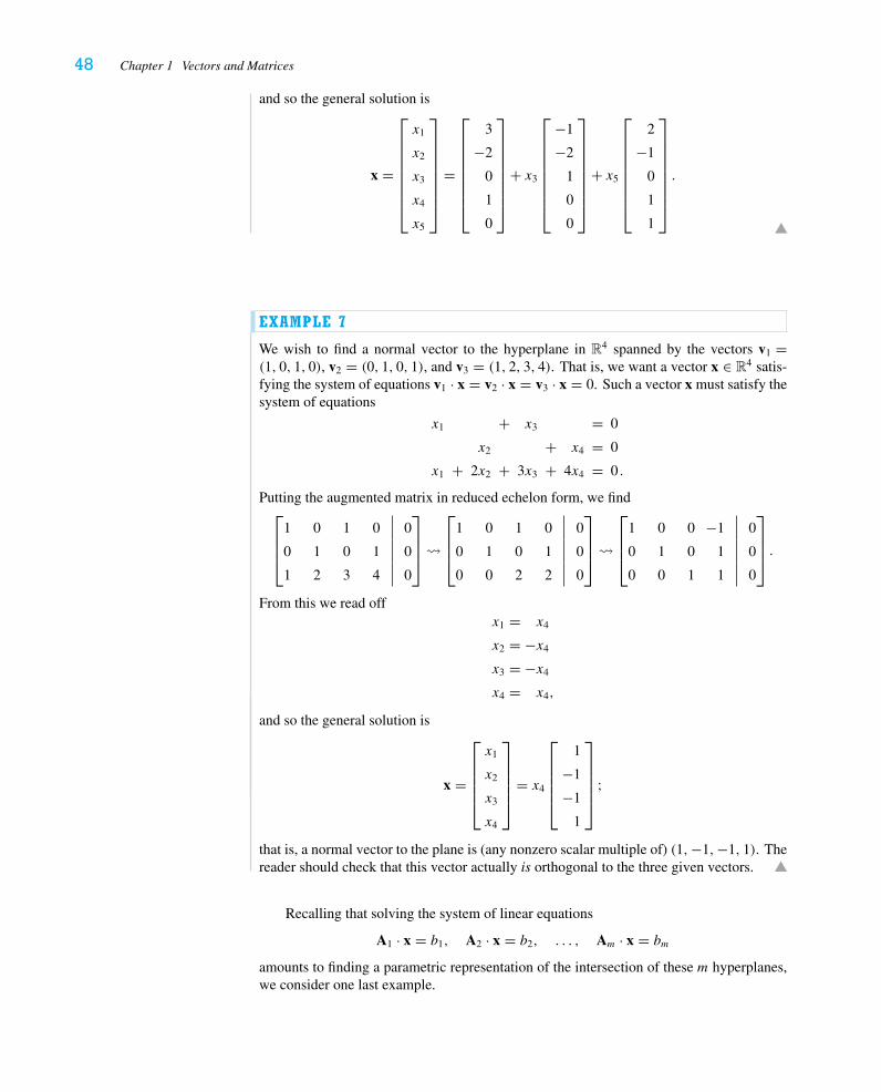
48 Chapter 1 Vectors and Matrices
and so the general solution is
x =
⎡⎢⎢⎢⎢⎢⎢⎢⎣
x1
x2
x3
x4
x5
⎤⎥⎥⎥⎥⎥⎥⎥⎦
=
⎡⎢⎢⎢⎢⎢⎢⎢⎣
3
−2
0
1
0
⎤⎥⎥⎥⎥⎥⎥⎥⎦
+ x3
⎡⎢⎢⎢⎢⎢⎢⎢⎣
−1
−2
1
0
0
⎤⎥⎥⎥⎥⎥⎥⎥⎦
+ x5
⎡⎢⎢⎢⎢⎢⎢⎢⎣
2
−1
0
1
1
⎤⎥⎥⎥⎥⎥⎥⎥⎦.
EXAMPLE 7
We wish to find a normal vector to the hyperplane in R4 spanned by the vectors v1 =(1, 0, 1, 0), v2 = (0, 1, 0, 1), and v3 = (1, 2, 3, 4). That is, we want a vector x ∈ R4 satis-fying the system of equations v1 · x = v2 · x = v3 · x = 0. Such a vector x must satisfy thesystem of equations
x1 + x3 = 0
x2 + x4 = 0
x1 + 2x2 + 3x3 + 4x4 = 0 .
Putting the augmented matrix in reduced echelon form, we find⎡⎢⎢⎣
1 0 1 0 0
0 1 0 1 0
1 2 3 4 0
⎤⎥⎥⎦�
⎡⎢⎢⎣
1 0 1 0 0
0 1 0 1 0
0 0 2 2 0
⎤⎥⎥⎦ �
⎡⎢⎢⎣
1 0 0 −1 0
0 1 0 1 0
0 0 1 1 0
⎤⎥⎥⎦ .
From this we read offx1 = x4
x2 = −x4
x3 = −x4
x4 = x4,
and so the general solution is
x =
⎡⎢⎢⎢⎢⎣
x1
x2
x3
x4
⎤⎥⎥⎥⎥⎦
= x4
⎡⎢⎢⎢⎢⎣
1
−1
−1
1
⎤⎥⎥⎥⎥⎦
;
that is, a normal vector to the plane is (any nonzero scalar multiple of) (1,−1,−1, 1). Thereader should check that this vector actually is orthogonal to the three given vectors.
Recalling that solving the system of linear equations
A1 · x = b1, A2 · x = b2, . . . , Am · x = bm
amounts to finding a parametric representation of the intersection of these m hyperplanes,we consider one last example.
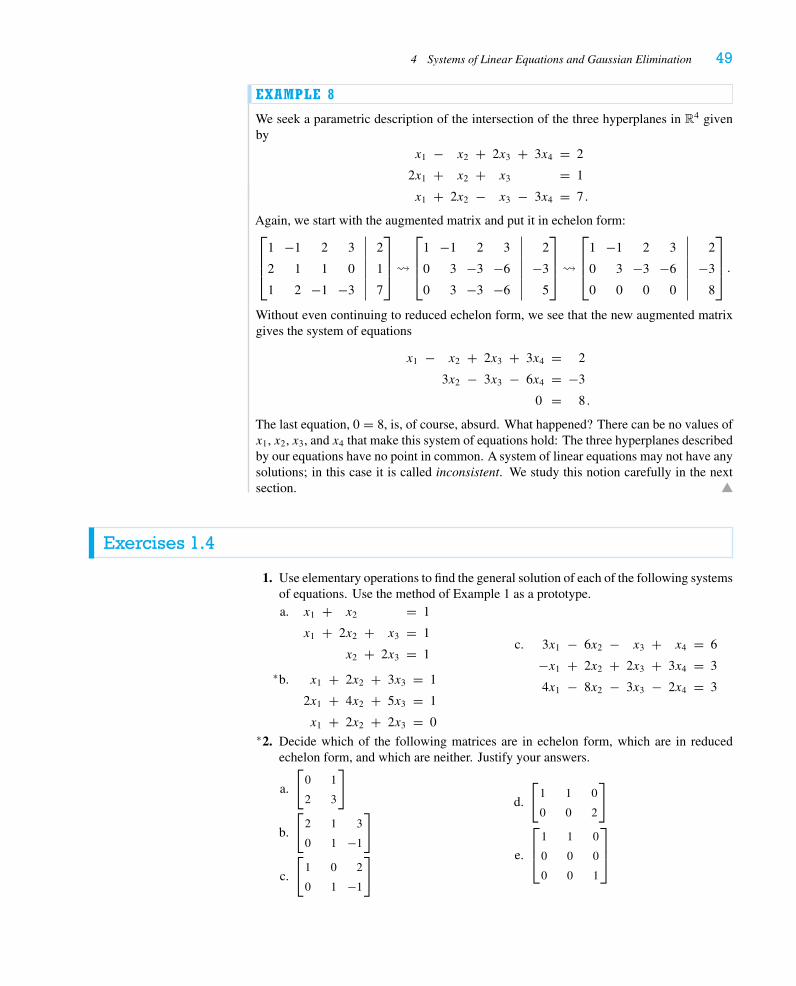
4 Systems of Linear Equations and Gaussian Elimination 49
EXAMPLE 8
We seek a parametric description of the intersection of the three hyperplanes in R4 givenby
x1 − x2 + 2x3 + 3x4 = 2
2x1 + x2 + x3 = 1
x1 + 2x2 − x3 − 3x4 = 7 .
Again, we start with the augmented matrix and put it in echelon form:⎡⎢⎢⎣
1 −1 2 3 2
2 1 1 0 1
1 2 −1 −3 7
⎤⎥⎥⎦�
⎡⎢⎢⎣
1 −1 2 3 2
0 3 −3 −6 −3
0 3 −3 −6 5
⎤⎥⎥⎦ �
⎡⎢⎢⎣
1 −1 2 3 2
0 3 −3 −6 −3
0 0 0 0 8
⎤⎥⎥⎦ .
Without even continuing to reduced echelon form, we see that the new augmented matrixgives the system of equations
x1 − x2 + 2x3 + 3x4 = 2
3x2 − 3x3 − 6x4 = −3
0 = 8 .
The last equation, 0 = 8, is, of course, absurd. What happened? There can be no values ofx1, x2, x3, and x4 that make this system of equations hold: The three hyperplanes describedby our equations have no point in common. A system of linear equations may not have anysolutions; in this case it is called inconsistent. We study this notion carefully in the nextsection.
Exercises 1.4
1. Use elementary operations to find the general solution of each of the following systemsof equations. Use the method of Example 1 as a prototype.a. x1 + x2 = 1
x1 + 2x2 + x3 = 1
x2 + 2x3 = 1
b.∗ x1 + 2x2 + 3x3 = 1
2x1 + 4x2 + 5x3 = 1
x1 + 2x2 + 2x3 = 0
c. 3x1 − 6x2 − x3 + x4 = 6
−x1 + 2x2 + 2x3 + 3x4 = 3
4x1 − 8x2 − 3x3 − 2x4 = 3
2.∗ Decide which of the following matrices are in echelon form, which are in reducedechelon form, and which are neither. Justify your answers.
a.
[0 1
2 3
]
b.
[2 1 3
0 1 −1
]
c.
[1 0 2
0 1 −1
]
d.
[1 1 0
0 0 2
]
e.
⎡⎢⎣
1 1 0
0 0 0
0 0 1
⎤⎥⎦
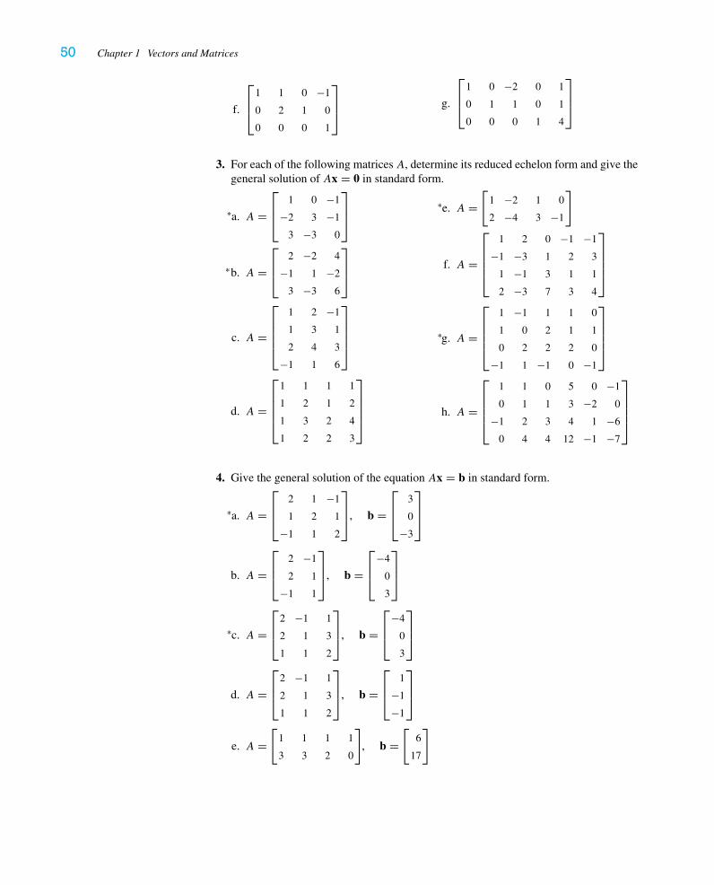
50 Chapter 1 Vectors and Matrices
f.
⎡⎢⎣
1 1 0 −1
0 2 1 0
0 0 0 1
⎤⎥⎦ g.
⎡⎢⎣
1 0 −2 0 1
0 1 1 0 1
0 0 0 1 4
⎤⎥⎦
3. For each of the following matrices A, determine its reduced echelon form and give thegeneral solution of Ax = 0 in standard form.
a.∗ A =⎡⎢⎣
1 0 −1
−2 3 −1
3 −3 0
⎤⎥⎦
b.∗ A =⎡⎢⎣
2 −2 4
−1 1 −2
3 −3 6
⎤⎥⎦
c. A =
⎡⎢⎢⎢⎣
1 2 −1
1 3 1
2 4 3
−1 1 6
⎤⎥⎥⎥⎦
d. A =
⎡⎢⎢⎢⎣
1 1 1 1
1 2 1 2
1 3 2 4
1 2 2 3
⎤⎥⎥⎥⎦
e.∗ A =[
1 −2 1 0
2 −4 3 −1
]
f. A =
⎡⎢⎢⎢⎣
1 2 0 −1 −1
−1 −3 1 2 3
1 −1 3 1 1
2 −3 7 3 4
⎤⎥⎥⎥⎦
g.∗ A =
⎡⎢⎢⎢⎣
1 −1 1 1 0
1 0 2 1 1
0 2 2 2 0
−1 1 −1 0 −1
⎤⎥⎥⎥⎦
h. A =
⎡⎢⎢⎢⎣
1 1 0 5 0 −1
0 1 1 3 −2 0
−1 2 3 4 1 −6
0 4 4 12 −1 −7
⎤⎥⎥⎥⎦
4. Give the general solution of the equation Ax = b in standard form.
a.∗ A =⎡⎢⎣
2 1 −1
1 2 1
−1 1 2
⎤⎥⎦, b =
⎡⎢⎣
3
0
−3
⎤⎥⎦
b. A =⎡⎢⎣
2 −1
2 1
−1 1
⎤⎥⎦, b =
⎡⎢⎣
−4
0
3
⎤⎥⎦
c.∗ A =⎡⎢⎣
2 −1 1
2 1 3
1 1 2
⎤⎥⎦, b =
⎡⎢⎣
−4
0
3
⎤⎥⎦
d. A =⎡⎢⎣
2 −1 1
2 1 3
1 1 2
⎤⎥⎦, b =
⎡⎢⎣
1
−1
−1
⎤⎥⎦
e. A =[
1 1 1 1
3 3 2 0
], b =
[6
17
]
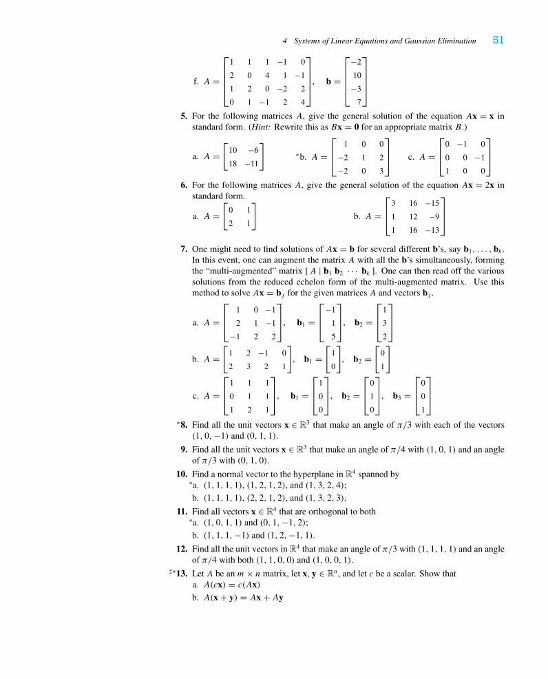
4 Systems of Linear Equations and Gaussian Elimination 51
f. A =
⎡⎢⎢⎢⎣
1 1 1 −1 0
2 0 4 1 −1
1 2 0 −2 2
0 1 −1 2 4
⎤⎥⎥⎥⎦, b =
⎡⎢⎢⎢⎣
−2
10
−3
7
⎤⎥⎥⎥⎦
5. For the following matrices A, give the general solution of the equation Ax = x instandard form. (Hint: Rewrite this as Bx = 0 for an appropriate matrix B.)
a. A =[
10 −6
18 −11
]b.∗ A =
⎡⎢⎣
1 0 0
−2 1 2
−2 0 3
⎤⎥⎦ c. A =
⎡⎢⎣
0 −1 0
0 0 −1
1 0 0
⎤⎥⎦
6. For the following matrices A, give the general solution of the equation Ax = 2x instandard form.
a. A =[
0 1
2 1
]b. A =
⎡⎢⎣
3 16 −15
1 12 −9
1 16 −13
⎤⎥⎦
7. One might need to find solutions of Ax = b for several different b’s, say b1, . . . ,bk .In this event, one can augment the matrix A with all the b’s simultaneously, formingthe “multi-augmented” matrix [A | b1 b2 · · · bk ]. One can then read off the varioussolutions from the reduced echelon form of the multi-augmented matrix. Use thismethod to solve Ax = bj for the given matrices A and vectors bj .
a. A =⎡⎢⎣
1 0 −1
2 1 −1
−1 2 2
⎤⎥⎦, b1 =
⎡⎢⎣
−1
1
5
⎤⎥⎦, b2 =
⎡⎢⎣
1
3
2
⎤⎥⎦
b. A =[
1 2 −1 0
2 3 2 1
], b1 =
[1
0
], b2 =
[0
1
]
c. A =⎡⎢⎣
1 1 1
0 1 1
1 2 1
⎤⎥⎦, b1 =
⎡⎢⎣
1
0
0
⎤⎥⎦, b2 =
⎡⎢⎣
0
1
0
⎤⎥⎦, b3 =
⎡⎢⎣
0
0
1
⎤⎥⎦
8.∗ Find all the unit vectors x ∈ R3 that make an angle of π/3 with each of the vectors(1, 0,−1) and (0, 1, 1).
9. Find all the unit vectors x ∈ R3 that make an angle of π/4 with (1, 0, 1) and an angleof π/3 with (0, 1, 0).
10. Find a normal vector to the hyperplane in R4 spanned bya.∗ (1, 1, 1, 1), (1, 2, 1, 2), and (1, 3, 2, 4);
b. (1, 1, 1, 1), (2, 2, 1, 2), and (1, 3, 2, 3).
11. Find all vectors x ∈ R4 that are orthogonal to botha.∗ (1, 0, 1, 1) and (0, 1,−1, 2);
b. (1, 1, 1,−1) and (1, 2,−1, 1).
12. Find all the unit vectors in R4 that make an angle of π/3 with (1, 1, 1, 1) and an angleof π/4 with both (1, 1, 0, 0) and (1, 0, 0, 1).
13.�∗ Let A be an m× n matrix, let x, y ∈ Rn, and let c be a scalar. Show thata. A(cx) = c(Ax)b. A(x + y) = Ax + Ay
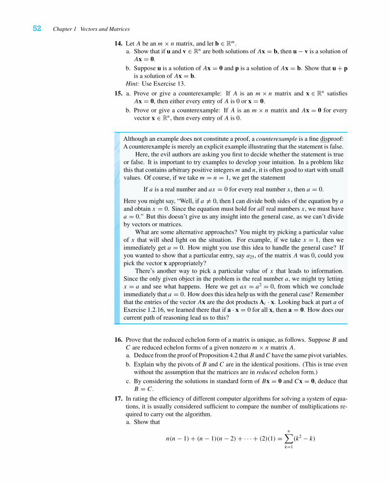
52 Chapter 1 Vectors and Matrices
14. Let A be an m× n matrix, and let b ∈ Rm.a. Show that if u and v ∈ Rn are both solutions of Ax = b, then u − v is a solution ofAx = 0.
b. Suppose u is a solution of Ax = 0 and p is a solution of Ax = b. Show that u + pis a solution of Ax = b.
Hint: Use Exercise 13.
15. a. Prove or give a counterexample: If A is an m× n matrix and x ∈ Rn satisfiesAx = 0, then either every entry of A is 0 or x = 0.
b. Prove or give a counterexample: If A is an m× n matrix and Ax = 0 for everyvector x ∈ Rn, then every entry of A is 0.
Although an example does not constitute a proof, a counterexample is a fine disproof:A counterexample is merely an explicit example illustrating that the statement is false.
Here, the evil authors are asking you first to decide whether the statement is trueor false. It is important to try examples to develop your intuition. In a problem likethis that contains arbitrary positive integersm and n, it is often good to start with smallvalues. Of course, if we take m = n = 1, we get the statement
If a is a real number and ax = 0 for every real number x, then a = 0.
Here you might say, “Well, if a �= 0, then I can divide both sides of the equation by aand obtain x = 0. Since the equation must hold for all real numbers x, we must havea = 0.” But this doesn’t give us any insight into the general case, as we can’t divideby vectors or matrices.
What are some alternative approaches? You might try picking a particular valueof x that will shed light on the situation. For example, if we take x = 1, then weimmediately get a = 0. How might you use this idea to handle the general case? Ifyou wanted to show that a particular entry, say a25, of the matrix A was 0, could youpick the vector x appropriately?
There’s another way to pick a particular value of x that leads to information.Since the only given object in the problem is the real number a, we might try lettingx = a and see what happens. Here we get ax = a2 = 0, from which we concludeimmediately that a = 0. How does this idea help us with the general case? Rememberthat the entries of the vector Ax are the dot products Ai · x. Looking back at part a ofExercise 1.2.16, we learned there that if a · x = 0 for all x, then a = 0. How does ourcurrent path of reasoning lead us to this?
16. Prove that the reduced echelon form of a matrix is unique, as follows. Suppose B andC are reduced echelon forms of a given nonzero m× n matrix A.a. Deduce from the proof of Proposition 4.2 thatB andC have the same pivot variables.
b. Explain why the pivots of B and C are in the identical positions. (This is true evenwithout the assumption that the matrices are in reduced echelon form.)
c. By considering the solutions in standard form of Bx = 0 and Cx = 0, deduce thatB = C.
17. In rating the efficiency of different computer algorithms for solving a system of equa-tions, it is usually considered sufficient to compare the number of multiplications re-quired to carry out the algorithm.a. Show that
n(n− 1)+ (n− 1)(n− 2)+ · · · + (2)(1) =n∑k=1
(k2 − k)
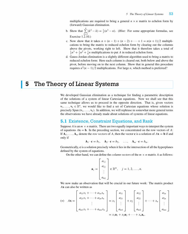
5 The Theory of Linear Systems 53
multiplications are required to bring a general n× n matrix to echelon form by(forward) Gaussian elimination.
b. Show thatn∑k=1(k2 − k) = 1
3 (n3 − n). (Hint: For some appropriate formulas, see
Exercise 1.2.10.)
c. Now show that it takes n+ (n− 1)+ (n− 2)+ · · · + 1 = n(n+ 1)/2 multipli-cations to bring the matrix to reduced echelon form by clearing out the columnsabove the pivots, working right to left. Show that it therefore takes a total of13n
3 + 12n
2 + 16n multiplications to put A in reduced echelon form.
d. Gauss-Jordan elimination is a slightly different algorithm used to bring a matrix toreduced echelon form: Here each column is cleared out, both below and above thepivot, before moving on to the next column. Show that in general this procedurerequires n2(n− 1)/2 multiplications. For large n, which method is preferred?
5 The Theory of Linear Systems
We developed Gaussian elimination as a technique for finding a parametric descriptionof the solutions of a system of linear Cartesian equations. Now we shall see that thissame technique allows us to proceed in the opposite direction. That is, given vectorsv1, . . . , vk ∈ Rn, we would like to find a set of Cartesian equations whose solution isprecisely Span (v1, . . . , vk). In addition, we will rephrase in somewhat more general termsthe observations we have already made about solutions of systems of linear equations.
5.1 Existence,Constraint Equations, and RankSupposeA is anm× nmatrix. There are two equally important ways to interpret the systemof equations Ax = b. In the preceding section, we concentrated on the row vectors of A:If A1, . . . ,Am denote the row vectors of A, then the vector c is a solution of Ax = b if andonly if
A1 · c = b1, A2 · c = b2, . . . , Am · c = bm.
Geometrically, c is a solution precisely when it lies in the intersection of all the hyperplanesdefined by the system of equations.
On the other hand, we can define the column vectors of them× nmatrixA as follows:
aj =
⎡⎢⎢⎢⎢⎢⎣
a1j
a2j
...
amj
⎤⎥⎥⎥⎥⎥⎦
∈ Rm, j = 1, 2, . . . , n.
We now make an observation that will be crucial in our future work: The matrix productAx can also be written as
Ax =
⎡⎢⎢⎢⎢⎢⎣
a11x1 + · · · + a1nxn
a21x1 + · · · + a2nxn...
am1x1 + · · · + amnxn
⎤⎥⎥⎥⎥⎥⎦
= x1
⎡⎢⎢⎢⎢⎢⎣
a11
a21
...
am1
⎤⎥⎥⎥⎥⎥⎦
+ x2
⎡⎢⎢⎢⎢⎢⎣
a12
a22
...
am2
⎤⎥⎥⎥⎥⎥⎦
+ · · · + xn
⎡⎢⎢⎢⎢⎢⎣
a1n
a2n
...
amn
⎤⎥⎥⎥⎥⎥⎦
(∗)
= x1a1 + x2a2 + · · · + xnan.
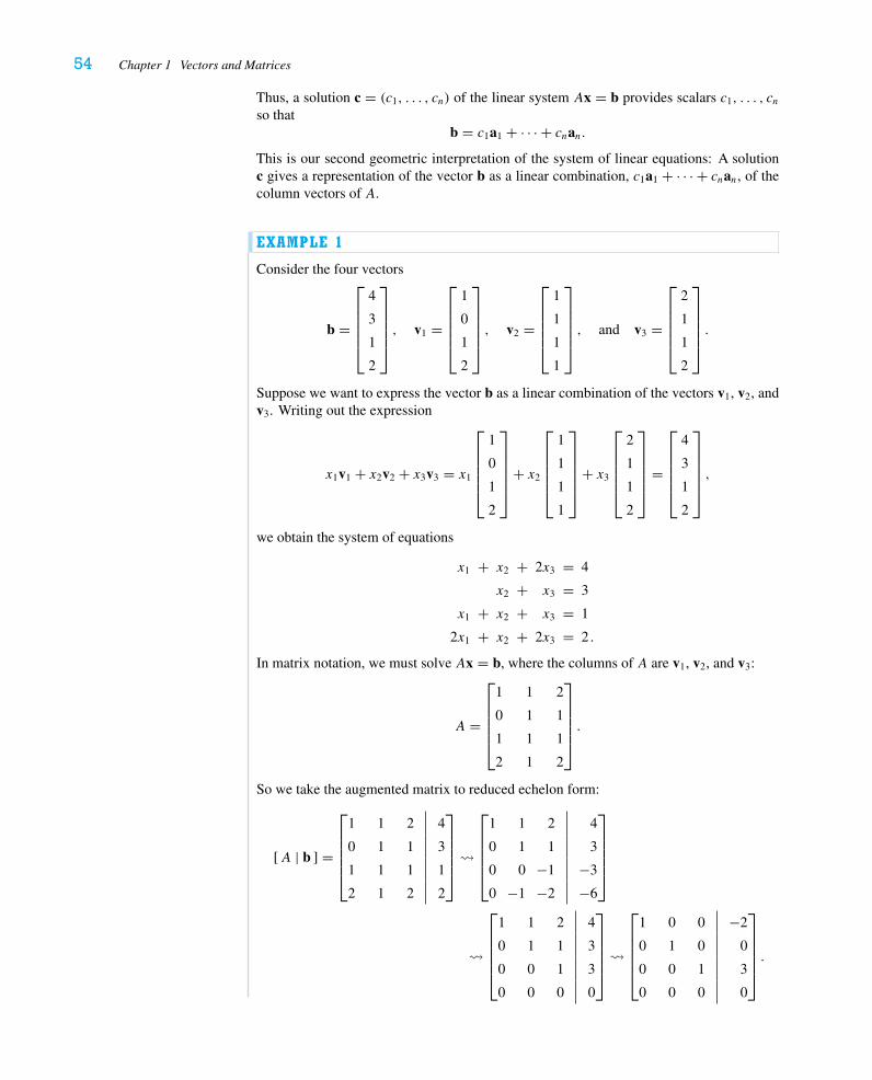
54 Chapter 1 Vectors and Matrices
Thus, a solution c = (c1, . . . , cn) of the linear system Ax = b provides scalars c1, . . . , cnso that
b = c1a1 + · · · + cnan.This is our second geometric interpretation of the system of linear equations: A solutionc gives a representation of the vector b as a linear combination, c1a1 + · · · + cnan, of thecolumn vectors of A.
EXAMPLE 1
Consider the four vectors
b =
⎡⎢⎢⎢⎢⎣
4
3
1
2
⎤⎥⎥⎥⎥⎦, v1 =
⎡⎢⎢⎢⎢⎣
1
0
1
2
⎤⎥⎥⎥⎥⎦, v2 =
⎡⎢⎢⎢⎢⎣
1
1
1
1
⎤⎥⎥⎥⎥⎦, and v3 =
⎡⎢⎢⎢⎢⎣
2
1
1
2
⎤⎥⎥⎥⎥⎦.
Suppose we want to express the vector b as a linear combination of the vectors v1, v2, andv3. Writing out the expression
x1v1 + x2v2 + x3v3 = x1
⎡⎢⎢⎢⎢⎣
1
0
1
2
⎤⎥⎥⎥⎥⎦
+ x2
⎡⎢⎢⎢⎢⎣
1
1
1
1
⎤⎥⎥⎥⎥⎦
+ x3
⎡⎢⎢⎢⎢⎣
2
1
1
2
⎤⎥⎥⎥⎥⎦
=
⎡⎢⎢⎢⎢⎣
4
3
1
2
⎤⎥⎥⎥⎥⎦,
we obtain the system of equations
x1 + x2 + 2x3 = 4
x2 + x3 = 3
x1 + x2 + x3 = 1
2x1 + x2 + 2x3 = 2 .
In matrix notation, we must solve Ax = b, where the columns of A are v1, v2, and v3:
A =
⎡⎢⎢⎢⎢⎣
1 1 2
0 1 1
1 1 1
2 1 2
⎤⎥⎥⎥⎥⎦.
So we take the augmented matrix to reduced echelon form:
[A | b ] =
⎡⎢⎢⎢⎢⎣
1 1 2 4
0 1 1 3
1 1 1 1
2 1 2 2
⎤⎥⎥⎥⎥⎦
�
⎡⎢⎢⎢⎢⎣
1 1 2 4
0 1 1 3
0 0 −1 −3
0 −1 −2 −6
⎤⎥⎥⎥⎥⎦
�
⎡⎢⎢⎢⎢⎣
1 1 2 4
0 1 1 3
0 0 1 3
0 0 0 0
⎤⎥⎥⎥⎥⎦
�
⎡⎢⎢⎢⎢⎣
1 0 0 −2
0 1 0 0
0 0 1 3
0 0 0 0
⎤⎥⎥⎥⎥⎦.
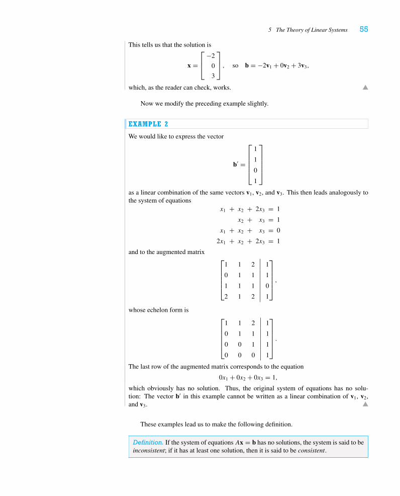
5 The Theory of Linear Systems 55
This tells us that the solution is
x =⎡⎢⎣
−2
0
3
⎤⎥⎦ , so b = −2v1 + 0v2 + 3v3,
which, as the reader can check, works.
Now we modify the preceding example slightly.
EXAMPLE 2
We would like to express the vector
b′ =
⎡⎢⎢⎢⎢⎣
1
1
0
1
⎤⎥⎥⎥⎥⎦
as a linear combination of the same vectors v1, v2, and v3. This then leads analogously tothe system of equations
x1 + x2 + 2x3 = 1
x2 + x3 = 1
x1 + x2 + x3 = 0
2x1 + x2 + 2x3 = 1
and to the augmented matrix⎡⎢⎢⎢⎢⎣
1 1 2 1
0 1 1 1
1 1 1 0
2 1 2 1
⎤⎥⎥⎥⎥⎦,
whose echelon form is⎡⎢⎢⎢⎢⎣
1 1 2 1
0 1 1 1
0 0 1 1
0 0 0 1
⎤⎥⎥⎥⎥⎦.
The last row of the augmented matrix corresponds to the equation
0x1 + 0x2 + 0x3 = 1,
which obviously has no solution. Thus, the original system of equations has no solu-tion: The vector b′ in this example cannot be written as a linear combination of v1, v2,and v3.
These examples lead us to make the following definition.
Definition. If the system of equations Ax = b has no solutions, the system is said to beinconsistent; if it has at least one solution, then it is said to be consistent.
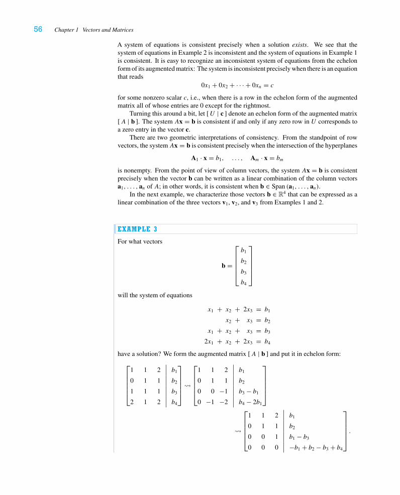
56 Chapter 1 Vectors and Matrices
A system of equations is consistent precisely when a solution exists. We see that thesystem of equations in Example 2 is inconsistent and the system of equations in Example 1is consistent. It is easy to recognize an inconsistent system of equations from the echelonform of its augmented matrix: The system is inconsistent precisely when there is an equationthat reads
0x1 + 0x2 + · · · + 0xn = c
for some nonzero scalar c, i.e., when there is a row in the echelon form of the augmentedmatrix all of whose entries are 0 except for the rightmost.
Turning this around a bit, let [U | c ] denote an echelon form of the augmented matrix[A | b ]. The system Ax = b is consistent if and only if any zero row in U corresponds toa zero entry in the vector c.
There are two geometric interpretations of consistency. From the standpoint of rowvectors, the systemAx = b is consistent precisely when the intersection of the hyperplanes
A1 · x = b1, . . . , Am · x = bm
is nonempty. From the point of view of column vectors, the system Ax = b is consistentprecisely when the vector b can be written as a linear combination of the column vectorsa1, . . . , an of A; in other words, it is consistent when b ∈ Span (a1, . . . , an).
In the next example, we characterize those vectors b ∈ R4 that can be expressed as alinear combination of the three vectors v1, v2, and v3 from Examples 1 and 2.
EXAMPLE 3
For what vectors
b =
⎡⎢⎢⎢⎢⎣
b1
b2
b3
b4
⎤⎥⎥⎥⎥⎦
will the system of equations
x1 + x2 + 2x3 = b1
x2 + x3 = b2
x1 + x2 + x3 = b3
2x1 + x2 + 2x3 = b4
have a solution? We form the augmented matrix [A | b ] and put it in echelon form:
⎡⎢⎢⎢⎢⎣
1 1 2 b1
0 1 1 b2
1 1 1 b3
2 1 2 b4
⎤⎥⎥⎥⎥⎦
�
⎡⎢⎢⎢⎢⎣
1 1 2 b1
0 1 1 b2
0 0 −1 b3 − b1
0 −1 −2 b4 − 2b1
⎤⎥⎥⎥⎥⎦
�
⎡⎢⎢⎢⎢⎣
1 1 2 b1
0 1 1 b2
0 0 1 b1 − b3
0 0 0 −b1 + b2 − b3 + b4
⎤⎥⎥⎥⎥⎦.
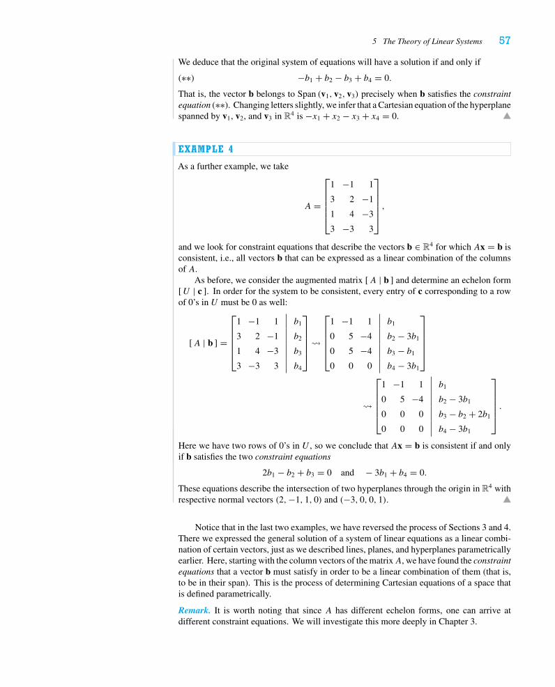
5 The Theory of Linear Systems 57
We deduce that the original system of equations will have a solution if and only if
(∗∗) −b1 + b2 − b3 + b4 = 0.
That is, the vector b belongs to Span (v1, v2, v3) precisely when b satisfies the constraintequation (∗∗). Changing letters slightly, we infer that a Cartesian equation of the hyperplanespanned by v1, v2, and v3 in R4 is −x1 + x2 − x3 + x4 = 0.
EXAMPLE 4
As a further example, we take
A =
⎡⎢⎢⎢⎢⎣
1 −1 1
3 2 −1
1 4 −3
3 −3 3
⎤⎥⎥⎥⎥⎦,
and we look for constraint equations that describe the vectors b ∈ R4 for which Ax = b isconsistent, i.e., all vectors b that can be expressed as a linear combination of the columnsof A.
As before, we consider the augmented matrix [A | b ] and determine an echelon form[U | c ]. In order for the system to be consistent, every entry of c corresponding to a rowof 0’s in U must be 0 as well:
[A | b ] =
⎡⎢⎢⎢⎢⎣
1 −1 1 b1
3 2 −1 b2
1 4 −3 b3
3 −3 3 b4
⎤⎥⎥⎥⎥⎦
�
⎡⎢⎢⎢⎢⎣
1 −1 1 b1
0 5 −4 b2 − 3b1
0 5 −4 b3 − b1
0 0 0 b4 − 3b1
⎤⎥⎥⎥⎥⎦
�
⎡⎢⎢⎢⎢⎣
1 −1 1 b1
0 5 −4 b2 − 3b1
0 0 0 b3 − b2 + 2b1
0 0 0 b4 − 3b1
⎤⎥⎥⎥⎥⎦.
Here we have two rows of 0’s in U , so we conclude that Ax = b is consistent if and onlyif b satisfies the two constraint equations
2b1 − b2 + b3 = 0 and − 3b1 + b4 = 0.
These equations describe the intersection of two hyperplanes through the origin in R4 withrespective normal vectors (2,−1, 1, 0) and (−3, 0, 0, 1).
Notice that in the last two examples, we have reversed the process of Sections 3 and 4.There we expressed the general solution of a system of linear equations as a linear combi-nation of certain vectors, just as we described lines, planes, and hyperplanes parametricallyearlier. Here, starting with the column vectors of the matrixA, we have found the constraintequations that a vector b must satisfy in order to be a linear combination of them (that is,to be in their span). This is the process of determining Cartesian equations of a space thatis defined parametrically.
Remark. It is worth noting that since A has different echelon forms, one can arrive atdifferent constraint equations. We will investigate this more deeply in Chapter 3.
58 Chapter 1 Vectors and Matrices
EXAMPLE 5
Find a Cartesian equation of the plane in R3 given parametrically by
x =
⎡⎢⎢⎣
1
2
1
⎤⎥⎥⎦+ s
⎡⎢⎢⎣
1
0
1
⎤⎥⎥⎦+ t
⎡⎢⎢⎣
2
1
1
⎤⎥⎥⎦ .
We ask which vectors b = (b1, b2, b3) can be written in the form⎡⎢⎢⎣
1
2
1
⎤⎥⎥⎦+ s
⎡⎢⎢⎣
1
0
1
⎤⎥⎥⎦+ t
⎡⎢⎢⎣
2
1
1
⎤⎥⎥⎦ =
⎡⎢⎢⎣b1
b2
b3
⎤⎥⎥⎦ .
This system of equations can be rewritten as⎡⎢⎢⎣
1 2
0 1
1 1
⎤⎥⎥⎦[s
t
]=
⎡⎢⎢⎣b1 − 1
b2 − 2
b3 − 1
⎤⎥⎥⎦ ,
and so we want to know when this system of equations is consistent. Reducing the aug-mented matrix to echelon form, we have
⎡⎢⎢⎣
1 2 b1 − 1
0 1 b2 − 2
1 1 b3 − 1
⎤⎥⎥⎦�
⎡⎢⎢⎣
1 2 b1 − 1
0 1 b2 − 2
0 0 b3 − b1 + b2 − 2
⎤⎥⎥⎦ .
Thus, the constraint equation is −b1 + b2 + b3 − 2 = 0. A Cartesian equation of the givenplane is x1 − x2 − x3 = −2.
In general, given an m× n matrix, we might wonder how many conditions a vectorb ∈ Rm must satisfy in order to be a linear combination of the columns of A. From theprocedure we’ve just followed, the answer is quite clear: Each row of 0’s in the echelonform of A contributes one constraint. This leads us to our next definition.
Definition. The rank of a matrixA is the number of nonzero rows (the number of pivots)in any echelon form of A. It is usually denoted by r .
Then the number of rows of 0’s in the echelon form is m− r , and b must satisfy m− rconstraint equations. Note that it is a consequence of Proposition 4.2 that the rank of amatrix is well-defined, i.e., independent of the choice of echelon form.
Now, given a system of m linear equations in n variables, let A denote its coefficientmatrix and r the rank of A. We summarize the above remarks as follows.
Proposition 5.1. The linear system Ax = b is consistent if and only if the rank of theaugmented matrix [A | b ] equals the rank of A. In particular, when the rank of A equalsm, the system Ax = b will be consistent for all vectors b ∈ Rm.
Proof. Let [U | c ] denote the echelon form of the augmented matrix [A | b ]. We knowthatAx = b is consistent if and only if any zero row in U corresponds to a zero entry in thevector c, which occurs if and only if the number of nonzero rows in the augmented matrix
5 The Theory of Linear Systems 59
[U | c ] equals the number of nonzero rows in U , i.e., the rank of A. When r = m, there isno row of 0’s in U and hence no possibility of inconsistency.
5.2 Uniqueness and Nonuniqueness of SolutionsWe now turn our attention to the question of how many solutions a given consistent systemof equations has. Our experience with solving systems of equations in Sections 3 and 4suggests that the solutions of a consistent linear system Ax = b are intimately related tothe solutions of the system Ax = 0.
Definition.A systemAx = b of linear equations is called inhomogeneous when b �= 0;the corresponding equation Ax = 0 is called the associated homogeneous system.
To relate the solutions of the inhomogeneous systemAx = b and those of the associatedhomogeneous system Ax = 0, we need the following fundamental algebraic observation.
Proposition 5.2. Let A be an m× n matrix and let x, y ∈ Rn. Then
A(x + y) = Ax + Ay.
(This is called the distributive property of matrix multiplication.)
Proof. Recall that, by definition, the i th entry of the product Ax is equal to the dot productAi · x. The distributive property of dot product (the last property listed in Proposition 2.1)dictates that
Ai · (x + y) = Ai · x + Ai · y,
and so the i th entry of A(x + y) equals the i th entry of Ax + Ay. Since this holds for alli = 1, . . . , m, the vectors are equal.
This argument establishes the first part of the following theorem.
Theorem 5.3. Assume the systemAx = b is consistent, and let u1 be a particular solution.15
Then all the solutions are of the form
u = u1 + v
for some solution v of the associated homogeneous system Ax = 0.
Proof. First we observe that any such vector u is a solution of Ax = b. Using Proposition5.2, we have
Au = A(u1 + v) = Au1 + Av = b + 0 = b.
Conversely, every solution of Ax = b can be written in this form, for if u is an arbitrarysolution of Ax = b, then, by distributivity again,
A(u − u1) = Au − Au1 = b − b = 0,
so v = u − u1 is a solution of the associated homogeneous system; now we just solve foru, obtaining u = u1 + v, as required.
Remark. As Figure 5.1 suggests, when the inhomogeneous system Ax = b is consistent,its solutions are obtained by translating the set of solutions of the associated homogeneous
15This is classical terminology for any single solution of the inhomogeneous system. There need not be anythingspecial about it. In Example 5 on p. 44, we saw a way to pick a particular particular solution.
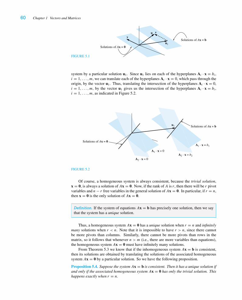
60 Chapter 1 Vectors and Matrices
FIGURE 5.1
uv
v
Solutions of Ax = 0
Solutions of Ax = bu1
system by a particular solution u1. Since u1 lies on each of the hyperplanes Ai · x = bi ,i = 1, . . . , m, we can translate each of the hyperplanes Ai · x = 0, which pass through theorigin, by the vector u1. Thus, translating the intersection of the hyperplanes Ai · x = 0,i = 1, . . . , m, by the vector u1 gives us the intersection of the hyperplanes Ai · x = bi ,i = 1, . . . , m, as indicated in Figure 5.2.
Solutions of Ax = 0
Solutions of Ax = bu1
A1 · x = b1
A2 · x = b2
A1 · x = 0
A2 · x = 0
FIGURE 5.2
Of course, a homogeneous system is always consistent, because the trivial solution,x = 0, is always a solution of Ax = 0. Now, if the rank of A is r , then there will be r pivotvariables and n− r free variables in the general solution ofAx = 0. In particular, if r = n,then x = 0 is the only solution of Ax = 0.
Definition. If the system of equations Ax = b has precisely one solution, then we saythat the system has a unique solution.
Thus, a homogeneous system Ax = 0 has a unique solution when r = n and infinitelymany solutions when r < n. Note that it is impossible to have r > n, since there cannotbe more pivots than columns. Similarly, there cannot be more pivots than rows in thematrix, so it follows that whenever n > m (i.e., there are more variables than equations),the homogeneous system Ax = 0 must have infinitely many solutions.
From Theorem 5.3 we know that if the inhomogeneous system Ax = b is consistent,then its solutions are obtained by translating the solutions of the associated homogeneoussystem Ax = 0 by a particular solution. So we have the following proposition.
Proposition 5.4. Suppose the system Ax = b is consistent. Then it has a unique solution ifand only if the associated homogeneous system Ax = 0 has only the trivial solution. Thishappens exactly when r = n.
5 The Theory of Linear Systems 61
We conclude this discussion with an important special case. It is natural to ask whenthe inhomogeneous system Ax = b has a unique solution for every b ∈ Rm. From Propo-sition 5.1 we infer that for the system always to be consistent, we must have r = m; fromProposition 5.4 we infer that for solutions to be unique, we must have r = n. And so wesee that we can have both conditions only when r = m = n.
Definition. An n× n matrix of rank r = n is called nonsingular. An n× n matrix ofrank r < n is called singular.
We observe that an n× n matrix is nonsingular if and only if there is a pivot in each row,hence in each column, of its echelon form. Thus, its reduced echelon form must be then× n matrix ⎡
⎢⎢⎢⎢⎢⎢⎢⎢⎣
1
1
0. . .
01
1
⎤⎥⎥⎥⎥⎥⎥⎥⎥⎦.
It seems silly to remark that when m = n, if r = n, then r = m, and conversely. Butthe following result, which will be extremely important in the next few chapters, is animmediate consequence of this observation.
Proposition 5.5. Let A be an n× n matrix. The following are equivalent:
1. A is nonsingular.
2. Ax = 0 has only the trivial solution.
3. For every b ∈ Rn, the equation Ax = b has a solution (indeed, a uniquesolution).
Exercises 1.5
1.∗ By solving a system of equations, find the linear combination of the vectors v1 =⎡⎢⎣
1
0
−1
⎤⎥⎦,
v2 =⎡⎢⎣
0
1
2
⎤⎥⎦, v3 =
⎡⎢⎣
2
1
1
⎤⎥⎦ that gives b =
⎡⎢⎣
3
0
−2
⎤⎥⎦.
2.∗ For each of the following vectors b ∈ R4, decide whether b is a linear combination of
v1 =
⎡⎢⎢⎢⎣
1
0
1
−2
⎤⎥⎥⎥⎦, v2 =
⎡⎢⎢⎢⎣
0
−1
0
1
⎤⎥⎥⎥⎦, and v3 =
⎡⎢⎢⎢⎣
1
−2
1
0
⎤⎥⎥⎥⎦.
a. b =
⎡⎢⎢⎢⎣
1
1
1
1
⎤⎥⎥⎥⎦ b. b =
⎡⎢⎢⎢⎣
1
−1
1
−1
⎤⎥⎥⎥⎦ c. b =
⎡⎢⎢⎢⎣
1
1
0
−2
⎤⎥⎥⎥⎦
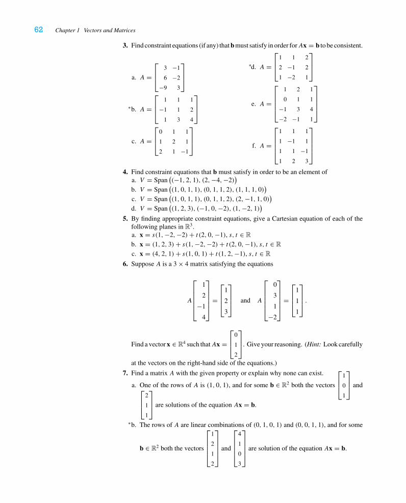
62 Chapter 1 Vectors and Matrices
3. Find constraint equations (if any) that b must satisfy in order forAx = b to be consistent.
a. A =⎡⎢⎣
3 −1
6 −2
−9 3
⎤⎥⎦
b.∗ A =⎡⎢⎣
1 1 1
−1 1 2
1 3 4
⎤⎥⎦
c. A =⎡⎢⎣
0 1 1
1 2 1
2 1 −1
⎤⎥⎦
d.∗ A =⎡⎢⎣
1 1 2
2 −1 2
1 −2 1
⎤⎥⎦
e. A =
⎡⎢⎢⎢⎣
1 2 1
0 1 1
−1 3 4
−2 −1 1
⎤⎥⎥⎥⎦
f. A =
⎡⎢⎢⎢⎣
1 1 1
1 −1 1
1 1 −1
1 2 3
⎤⎥⎥⎥⎦
4. Find constraint equations that b must satisfy in order to be an element ofa. V = Span
((−1, 2, 1), (2,−4,−2)
)b. V = Span
((1, 0, 1, 1), (0, 1, 1, 2), (1, 1, 1, 0)
)c. V = Span
((1, 0, 1, 1), (0, 1, 1, 2), (2,−1, 1, 0)
)d. V = Span
((1, 2, 3), (−1, 0,−2), (1,−2, 1)
)
5. By finding appropriate constraint equations, give a Cartesian equation of each of thefollowing planes in R3.a. x = s(1,−2,−2)+ t (2, 0,−1), s, t ∈ R
b. x = (1, 2, 3)+ s(1,−2,−2)+ t (2, 0,−1), s, t ∈ R
c. x = (4, 2, 1)+ s(1, 0, 1)+ t (1, 2,−1), s, t ∈ R
6. Suppose A is a 3 × 4 matrix satisfying the equations
A
⎡⎢⎢⎢⎢⎣
1
2
−1
4
⎤⎥⎥⎥⎥⎦
=
⎡⎢⎢⎣
1
2
3
⎤⎥⎥⎦ and A
⎡⎢⎢⎢⎢⎣
0
3
1
−2
⎤⎥⎥⎥⎥⎦
=
⎡⎢⎢⎣
1
1
1
⎤⎥⎥⎦ .
Find a vector x ∈ R4 such thatAx =⎡⎢⎣
0
1
2
⎤⎥⎦. Give your reasoning. (Hint: Look carefully
at the vectors on the right-hand side of the equations.)
7. Find a matrix A with the given property or explain why none can exist.
a. One of the rows of A is (1, 0, 1), and for some b ∈ R2 both the vectors
⎡⎢⎣
1
0
1
⎤⎥⎦ and⎡
⎢⎣2
1
1
⎤⎥⎦ are solutions of the equation Ax = b.
b.∗ The rows of A are linear combinations of (0, 1, 0, 1) and (0, 0, 1, 1), and for some
b ∈ R2 both the vectors
⎡⎢⎢⎢⎣
1
2
1
2
⎤⎥⎥⎥⎦ and
⎡⎢⎢⎢⎣
4
1
0
3
⎤⎥⎥⎥⎦ are solution of the equation Ax = b.
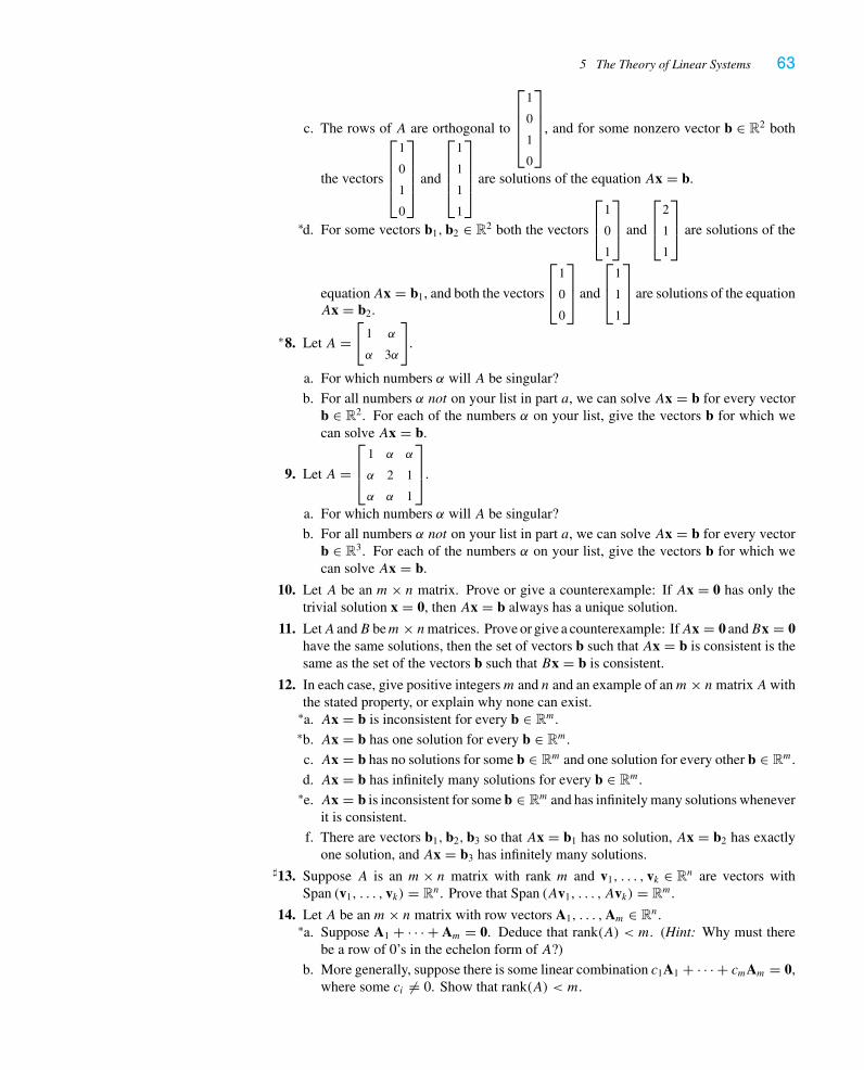
5 The Theory of Linear Systems 63
c. The rows of A are orthogonal to
⎡⎢⎢⎢⎣
1
0
1
0
⎤⎥⎥⎥⎦, and for some nonzero vector b ∈ R2 both
the vectors
⎡⎢⎢⎢⎣
1
0
1
0
⎤⎥⎥⎥⎦ and
⎡⎢⎢⎢⎣
1
1
1
1
⎤⎥⎥⎥⎦ are solutions of the equation Ax = b.
d.∗ For some vectors b1, b2 ∈ R2 both the vectors
⎡⎢⎣
1
0
1
⎤⎥⎦ and
⎡⎢⎣
2
1
1
⎤⎥⎦ are solutions of the
equationAx = b1, and both the vectors
⎡⎢⎣
1
0
0
⎤⎥⎦ and
⎡⎢⎣
1
1
1
⎤⎥⎦ are solutions of the equation
Ax = b2.
8.∗ Let A =[
1 α
α 3α
].
a. For which numbers α will A be singular?
b. For all numbers α not on your list in part a, we can solve Ax = b for every vectorb ∈ R2. For each of the numbers α on your list, give the vectors b for which wecan solve Ax = b.
9. Let A =⎡⎢⎣
1 α α
α 2 1
α α 1
⎤⎥⎦.
a. For which numbers α will A be singular?
b. For all numbers α not on your list in part a, we can solve Ax = b for every vectorb ∈ R3. For each of the numbers α on your list, give the vectors b for which wecan solve Ax = b.
10. Let A be an m× n matrix. Prove or give a counterexample: If Ax = 0 has only thetrivial solution x = 0, then Ax = b always has a unique solution.
11. LetA andB bem× nmatrices. Prove or give a counterexample: IfAx = 0 andBx = 0have the same solutions, then the set of vectors b such that Ax = b is consistent is thesame as the set of the vectors b such that Bx = b is consistent.
12. In each case, give positive integersm and n and an example of anm× nmatrixAwiththe stated property, or explain why none can exist.a.∗ Ax = b is inconsistent for every b ∈ Rm.
b.∗ Ax = b has one solution for every b ∈ Rm.
c. Ax = b has no solutions for some b ∈ Rm and one solution for every other b ∈ Rm.
d. Ax = b has infinitely many solutions for every b ∈ Rm.
e.∗ Ax = b is inconsistent for some b ∈ Rm and has infinitely many solutions wheneverit is consistent.
f. There are vectors b1, b2, b3 so that Ax = b1 has no solution, Ax = b2 has exactlyone solution, and Ax = b3 has infinitely many solutions.
13.� Suppose A is an m× n matrix with rank m and v1, . . . , vk ∈ Rn are vectors withSpan (v1, . . . , vk) = Rn. Prove that Span (Av1, . . . , Avk) = Rm.
14. Let A be an m× n matrix with row vectors A1, . . . ,Am ∈ Rn.a.∗ Suppose A1 + · · · + Am = 0. Deduce that rank(A) < m. (Hint: Why must there
be a row of 0’s in the echelon form of A?)
b. More generally, suppose there is some linear combination c1A1 + · · · + cmAm = 0,where some ci �= 0. Show that rank(A) < m.
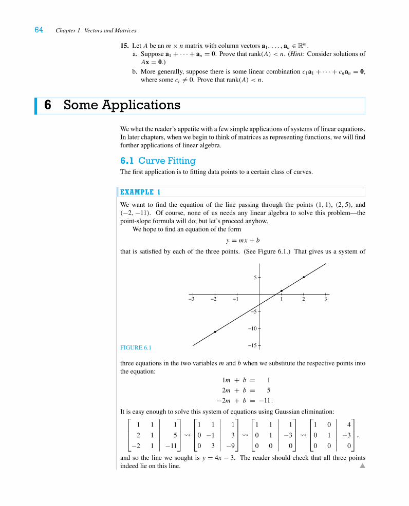
64 Chapter 1 Vectors and Matrices
15. Let A be an m× n matrix with column vectors a1, . . . , an ∈ Rm.a. Suppose a1 + · · · + an = 0. Prove that rank(A) < n. (Hint: Consider solutions ofAx = 0.)
b. More generally, suppose there is some linear combination c1a1 + · · · + cnan = 0,where some ci �= 0. Prove that rank(A) < n.
6 Some Applications
We whet the reader’s appetite with a few simple applications of systems of linear equations.In later chapters, when we begin to think of matrices as representing functions, we will findfurther applications of linear algebra.
6.1 Curve FittingThe first application is to fitting data points to a certain class of curves.
EXAMPLE 1
We want to find the equation of the line passing through the points (1, 1), (2, 5), and(−2,−11). Of course, none of us needs any linear algebra to solve this problem—thepoint-slope formula will do; but let’s proceed anyhow.
We hope to find an equation of the form
y = mx + bthat is satisfied by each of the three points. (See Figure 6.1.) That gives us a system of
FIGURE 6.1
−3 −2 −1 1 2 3
−15
−10
−5
5
three equations in the two variables m and b when we substitute the respective points intothe equation:
1m + b = 1
2m + b = 5
−2m + b = −11 .
It is easy enough to solve this system of equations using Gaussian elimination:⎡⎢⎢⎣
1 1 1
2 1 5
−2 1 −11
⎤⎥⎥⎦�
⎡⎢⎢⎣
1 1 1
0 −1 3
0 3 −9
⎤⎥⎥⎦�
⎡⎢⎢⎣
1 1 1
0 1 −3
0 0 0
⎤⎥⎥⎦ �
⎡⎢⎢⎣
1 0 4
0 1 −3
0 0 0
⎤⎥⎥⎦ ,
and so the line we sought is y = 4x − 3. The reader should check that all three pointsindeed lie on this line.
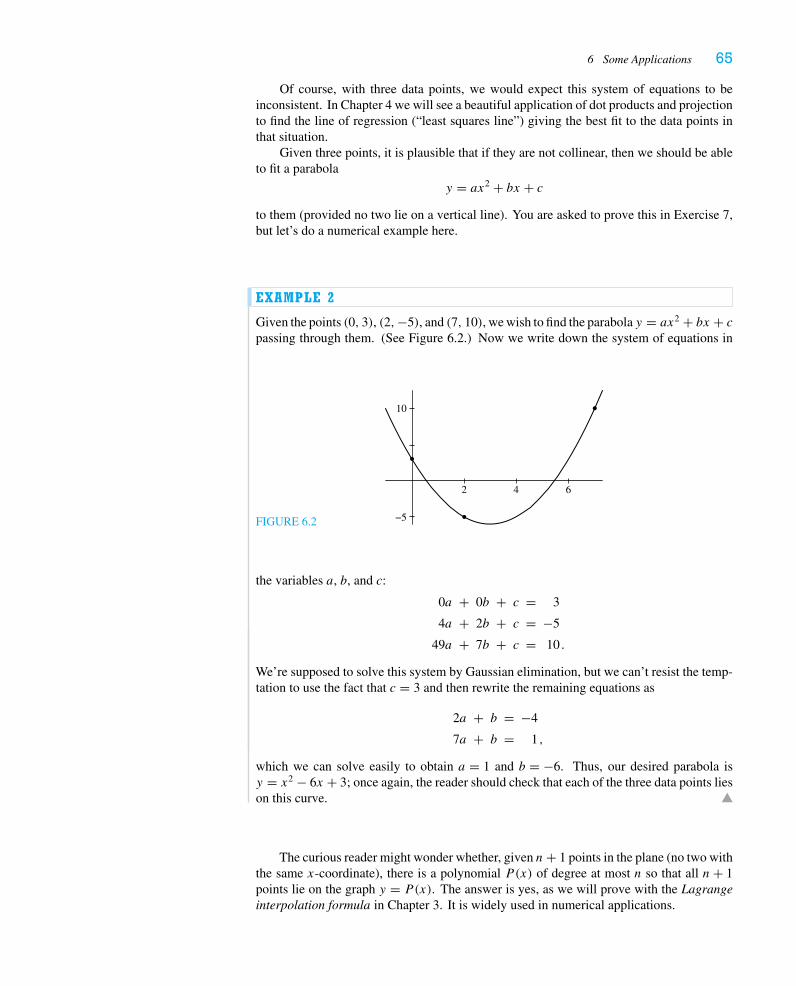
6 Some Applications 65
Of course, with three data points, we would expect this system of equations to beinconsistent. In Chapter 4 we will see a beautiful application of dot products and projectionto find the line of regression (“least squares line”) giving the best fit to the data points inthat situation.
Given three points, it is plausible that if they are not collinear, then we should be ableto fit a parabola
y = ax2 + bx + cto them (provided no two lie on a vertical line). You are asked to prove this in Exercise 7,but let’s do a numerical example here.
EXAMPLE 2
Given the points (0, 3), (2,−5), and (7, 10), we wish to find the parabola y = ax2 + bx + cpassing through them. (See Figure 6.2.) Now we write down the system of equations in
FIGURE 6.2
2 4 6
−5
10
the variables a, b, and c:
0a + 0b + c = 3
4a + 2b + c = −5
49a + 7b + c = 10 .
We’re supposed to solve this system by Gaussian elimination, but we can’t resist the temp-tation to use the fact that c = 3 and then rewrite the remaining equations as
2a + b = −4
7a + b = 1 ,
which we can solve easily to obtain a = 1 and b = −6. Thus, our desired parabola isy = x2 − 6x + 3; once again, the reader should check that each of the three data points lieson this curve.
The curious reader might wonder whether, given n+ 1 points in the plane (no two withthe same x-coordinate), there is a polynomial P(x) of degree at most n so that all n+ 1points lie on the graph y = P(x). The answer is yes, as we will prove with the Lagrangeinterpolation formula in Chapter 3. It is widely used in numerical applications.
66 Chapter 1 Vectors and Matrices
6.2 StoichiometryFor our next application, we recall the torture of balancing chemical equations in ourfreshman chemistry class. The name stoichiometry16 suggests that a chemist should bemeasuring how many moles of each reactant and product there are; the analysis of how acomplicated chemical reaction occurs as a sequence of certain simpler reactions is actuallyquite fascinating. Nevertheless, there is a fundamental mathematical issue of balancingthe number of atoms of each element on the two sides of the reaction, and this amountsto—surprise! surprise!—a system of linear equations.
EXAMPLE 3
Consider the chemical reaction
aH2O + bFe � cFe(OH)3 + dH2.
We wish to find the smallest positive integersa, b, c, andd for which the “equation balances.”Comparing the number of atoms of H, O, and Fe on either side of the reaction leads to thefollowing system of equations:
2a = 3c + 2d
a = 3c
b = c
Moving all the variables to the left side yields the homogeneous system
2a − 3c − 2d = 0
a − 3c = 0
b − c = 0 .
Applying Gaussian elimination to bring the coefficient matrix to reduced echelon form, wefind ⎡
⎢⎢⎣2 0 −3 −2
1 0 −3 0
0 1 −1 0
⎤⎥⎥⎦�
⎡⎢⎢⎣
1 0 0 −2
0 1 0 − 23
0 0 1 − 23
⎤⎥⎥⎦ .
That is, we have
a = 2d
b = 23d
c = 23d
d = d ,
and so we see that the solution consisting of the smallest positive integers will arise whend = 3, resulting in a = 6, b = c = 2. That is, we have the chemical equation
6H2O + 2Fe � 2Fe(OH)3 + 3H2.
16Indeed, the root is the Greek stoicheion, meaning “first principle” or “element.”
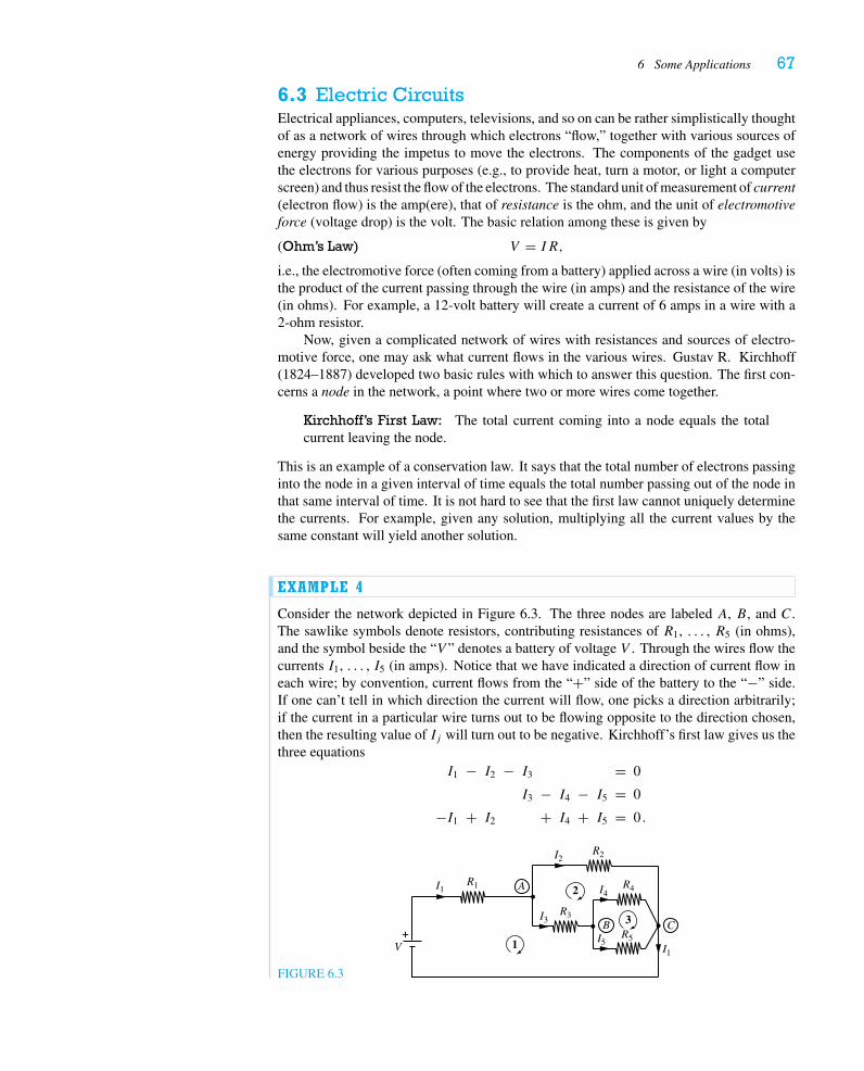
6 Some Applications 67
6.3 Electric CircuitsElectrical appliances, computers, televisions, and so on can be rather simplistically thoughtof as a network of wires through which electrons “flow,” together with various sources ofenergy providing the impetus to move the electrons. The components of the gadget usethe electrons for various purposes (e.g., to provide heat, turn a motor, or light a computerscreen) and thus resist the flow of the electrons. The standard unit of measurement of current(electron flow) is the amp(ere), that of resistance is the ohm, and the unit of electromotiveforce (voltage drop) is the volt. The basic relation among these is given by
(Ohm’s Law) V = IR,
i.e., the electromotive force (often coming from a battery) applied across a wire (in volts) isthe product of the current passing through the wire (in amps) and the resistance of the wire(in ohms). For example, a 12-volt battery will create a current of 6 amps in a wire with a2-ohm resistor.
Now, given a complicated network of wires with resistances and sources of electro-motive force, one may ask what current flows in the various wires. Gustav R. Kirchhoff(1824–1887) developed two basic rules with which to answer this question. The first con-cerns a node in the network, a point where two or more wires come together.
Kirchhoff’s First Law: The total current coming into a node equals the totalcurrent leaving the node.
This is an example of a conservation law. It says that the total number of electrons passinginto the node in a given interval of time equals the total number passing out of the node inthat same interval of time. It is not hard to see that the first law cannot uniquely determinethe currents. For example, given any solution, multiplying all the current values by thesame constant will yield another solution.
EXAMPLE 4
Consider the network depicted in Figure 6.3. The three nodes are labeled A, B, and C.The sawlike symbols denote resistors, contributing resistances of R1, . . . , R5 (in ohms),and the symbol beside the “V ” denotes a battery of voltage V . Through the wires flow thecurrents I1, . . . , I5 (in amps). Notice that we have indicated a direction of current flow ineach wire; by convention, current flows from the “+” side of the battery to the “−” side.If one can’t tell in which direction the current will flow, one picks a direction arbitrarily;if the current in a particular wire turns out to be flowing opposite to the direction chosen,then the resulting value of Ij will turn out to be negative. Kirchhoff’s first law gives us thethree equations
I1 − I2 − I3 = 0
I3 − I4 − I5 = 0
−I1 + I2 + I4 + I5 = 0 .
FIGURE 6.3
A
B C
V+
3
2
1
I2R2
R4
R5
R3
R1 I4
I3
I1
I5I1
68 Chapter 1 Vectors and Matrices
Since there are fewer equations than unknowns, this system of linear equations must haveinfinitely many solutions, just as we expect from the physics. Note that the third equationis clearly redundant, so we will discard it below.
To determine the currents completely, we need Kirchhoff’s second law, which concernsthe loops in a network. A loop is any path in the network starting and ending at the samenode. We have specified three “basic” loops in this example in the diagram.
Kirchhoff’s Second Law: The net voltage drop around a loop is zero. That is,the total “applied” voltage must equal the sum of the products IjRj for each wirein the loop.
EXAMPLE 5
We continue the analysis of Example 4. First, loop 1 has an external applied voltage V , so
R1I1 + R3I3 + R5I5 = V.
(We are writing the variables in this awkward order because we ultimately will be givenvalues ofRj and will want to solve for the currents Ij .) There is no external voltage in loop2, so the IR sum must be 0; i.e.,
R2I2 − R3I3 − R4I4 = 0.
Similarly, loop 3 gives
R4I4 − R5I5 = 0.
Of course, there are other loops in the circuit. The reader may find it interesting to noticethat any equation determined by another loop is a linear combination of the three equationswe’ve given, so that, in some sense, the three loops we chose are the only ones required.
Summarizing, we now have five equations in the five unknowns I1, . . . , I5:
I1 − I2 − I3 = 0
I3 − I4 − I5 = 0
R1I1 + R3I3 + R5I5 = V
R2I2 − R3I3 + R4I4 = 0
R4I4 − R5I5 = 0 .
One can solve this system for general values of R1, . . . , R5, and V , but it gets quite messy.Instead, let’s assign some specific values and solve the resulting system of linear equations.With
R1 = R3 = R4 = 2, R2 = R5 = 4, and V = 210,
after some work, we obtain the solution
I1 = 55, I2 = 25, I3 = 30, I4 = 20, I5 = 10.
6 Some Applications 69
Here are a few intermediate steps in the row reduction, for those who would like to checkour work: ⎡
⎢⎢⎢⎢⎢⎢⎢⎣
1 −1 −1 0 0 0
0 0 1 −1 −1 0
2 0 2 0 4 210
0 4 −2 −2 0 0
0 0 0 2 −4 0
⎤⎥⎥⎥⎥⎥⎥⎥⎦
�
⎡⎢⎢⎢⎢⎢⎢⎢⎣
1 −1 −1 0 0 0
0 0 1 −1 −1 0
0 2 −1 −1 0 0
0 0 0 1 −2 0
2 0 2 0 4 210
⎤⎥⎥⎥⎥⎥⎥⎥⎦
�
⎡⎢⎢⎢⎢⎢⎢⎢⎣
1 −1 −1 0 0 0
0 2 −1 −1 0 0
0 0 1 −1 −1 0
0 0 0 1 −2 0
0 0 0 0 21 210
⎤⎥⎥⎥⎥⎥⎥⎥⎦,
from which we deduce that I5 = 10, and the rest follows easily by back-substitution.
As a final remark, we add that this analysis can be applied to other types of networkproblems where there is a conservation law along with a linear relation between the “force”and the “rate of flow.” For example, when water flows in a network of pipes, the amount ofwater flowing into a joint must equal the amount flowing out (the analogue of Kirchhoff’sfirst law). Also, under a fixed amount of pressure, water will flow faster in a pipe withsmall cross section than in one with large cross section. Thus, inverse cross-sectional areacorresponds to resistance, and water pressure corresponds to voltage; we leave it to thereader to formulate the appropriate version of Kirchhoff’s second law. The reader may findit amusing to try to generalize these ideas to trucking networks, airplane scheduling, ormanufacturing problems. Also, see Section 5 of Chapter 3, where we take up Kirchhoff’slaws from a more conceptual viewpoint.
6.4 Difference Equations and Discrete DynamicalSystems
One of the most extensive applications of linear algebra is to the study of difference equa-tions, a discrete version of the differential equations you may have seen in calculus modelingcontinuous growth and natural phenomena.
EXAMPLE 6
The most basic problem involving population growth comes from simple compounding (sothe population is likely to be either rabbits or dollars in a bank account). If xk denotesthe population on day k, we may stipulate that the increase from day k to day k + 1, i.e.,
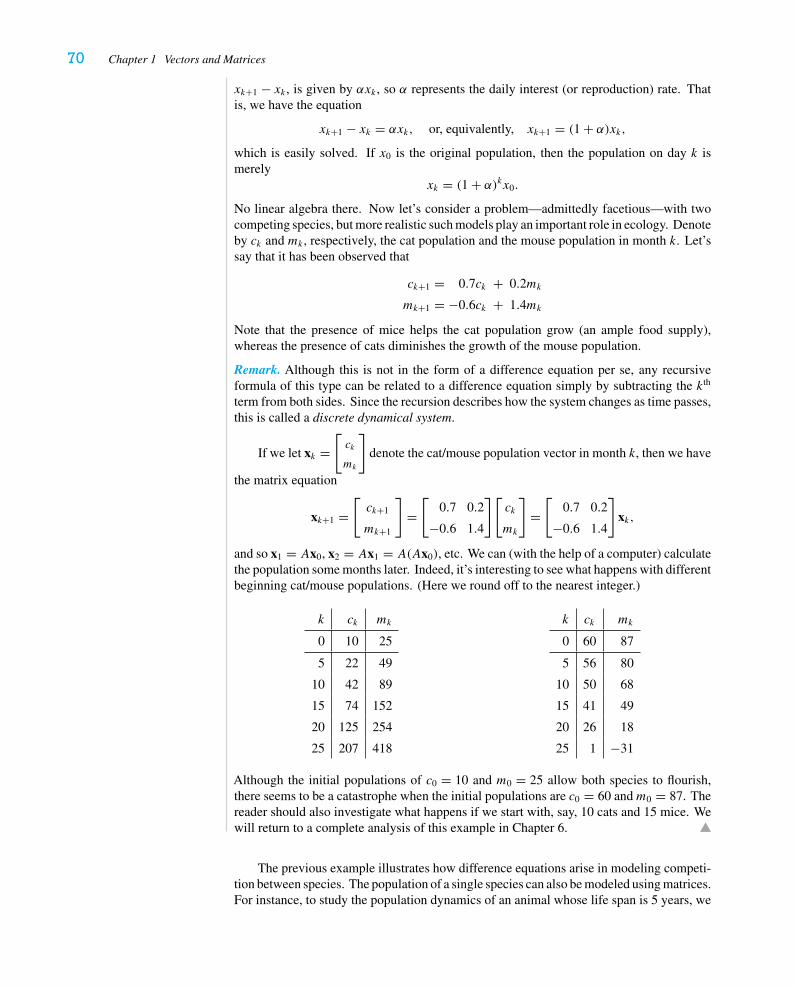
70 Chapter 1 Vectors and Matrices
xk+1 − xk , is given by αxk , so α represents the daily interest (or reproduction) rate. Thatis, we have the equation
xk+1 − xk = αxk, or, equivalently, xk+1 = (1 + α)xk,which is easily solved. If x0 is the original population, then the population on day k ismerely
xk = (1 + α)kx0.
No linear algebra there. Now let’s consider a problem—admittedly facetious—with twocompeting species, but more realistic such models play an important role in ecology. Denoteby ck and mk , respectively, the cat population and the mouse population in month k. Let’ssay that it has been observed that
ck+1 = 0.7ck + 0.2mk
mk+1 = −0.6ck + 1.4mk
Note that the presence of mice helps the cat population grow (an ample food supply),whereas the presence of cats diminishes the growth of the mouse population.
Remark. Although this is not in the form of a difference equation per se, any recursiveformula of this type can be related to a difference equation simply by subtracting the kth
term from both sides. Since the recursion describes how the system changes as time passes,this is called a discrete dynamical system.
If we let xk =[ck
mk
]denote the cat/mouse population vector in month k, then we have
the matrix equation
xk+1 =[ck+1
mk+1
]=[
0.7 0.2
−0.6 1.4
][ck
mk
]=[
0.7 0.2
−0.6 1.4
]xk,
and so x1 = Ax0, x2 = Ax1 = A(Ax0), etc. We can (with the help of a computer) calculatethe population some months later. Indeed, it’s interesting to see what happens with differentbeginning cat/mouse populations. (Here we round off to the nearest integer.)
k ck mk
0 10 25
5 22 49
10 42 89
15 74 152
20 125 254
25 207 418
k ck mk
0 60 87
5 56 80
10 50 68
15 41 49
20 26 18
25 1 −31
Although the initial populations of c0 = 10 and m0 = 25 allow both species to flourish,there seems to be a catastrophe when the initial populations are c0 = 60 andm0 = 87. Thereader should also investigate what happens if we start with, say, 10 cats and 15 mice. Wewill return to a complete analysis of this example in Chapter 6.
The previous example illustrates how difference equations arise in modeling competi-tion between species. The population of a single species can also be modeled using matrices.For instance, to study the population dynamics of an animal whose life span is 5 years, we
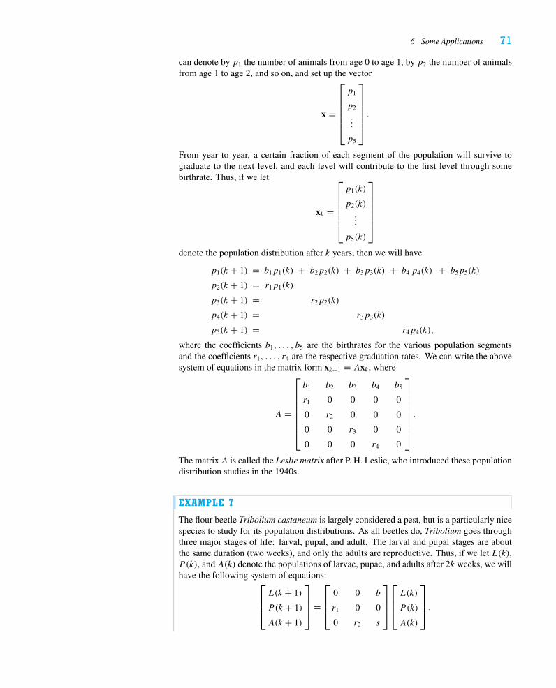
6 Some Applications 71
can denote by p1 the number of animals from age 0 to age 1, by p2 the number of animalsfrom age 1 to age 2, and so on, and set up the vector
x =
⎡⎢⎢⎢⎢⎢⎣
p1
p2
...
p5
⎤⎥⎥⎥⎥⎥⎦.
From year to year, a certain fraction of each segment of the population will survive tograduate to the next level, and each level will contribute to the first level through somebirthrate. Thus, if we let
xk =
⎡⎢⎢⎢⎢⎢⎣
p1(k)
p2(k)
...
p5(k)
⎤⎥⎥⎥⎥⎥⎦
denote the population distribution after k years, then we will have
p1(k + 1) = b1p1(k) + b2p2(k) + b3p3(k) + b4 p4(k) + b5p5(k)
p2(k + 1) = r1p1(k)
p3(k + 1) = r2p2(k)
p4(k + 1) = r3p3(k)
p5(k + 1) = r4p4(k),
where the coefficients b1, . . . , b5 are the birthrates for the various population segmentsand the coefficients r1, . . . , r4 are the respective graduation rates. We can write the abovesystem of equations in the matrix form xk+1 = Axk , where
A =
⎡⎢⎢⎢⎢⎢⎢⎢⎣
b1 b2 b3 b4 b5
r1 0 0 0 0
0 r2 0 0 0
0 0 r3 0 0
0 0 0 r4 0
⎤⎥⎥⎥⎥⎥⎥⎥⎦.
The matrix A is called the Leslie matrix after P. H. Leslie, who introduced these populationdistribution studies in the 1940s.
EXAMPLE 7
The flour beetle Tribolium castaneum is largely considered a pest, but is a particularly nicespecies to study for its population distributions. As all beetles do, Tribolium goes throughthree major stages of life: larval, pupal, and adult. The larval and pupal stages are aboutthe same duration (two weeks), and only the adults are reproductive. Thus, if we let L(k),P(k), and A(k) denote the populations of larvae, pupae, and adults after 2k weeks, we willhave the following system of equations:⎡
⎢⎢⎣L(k + 1)
P (k + 1)
A(k + 1)
⎤⎥⎥⎦ =
⎡⎢⎢⎣
0 0 b
r1 0 0
0 r2 s
⎤⎥⎥⎦
⎡⎢⎢⎣L(k)
P (k)
A(k)
⎤⎥⎥⎦ ,
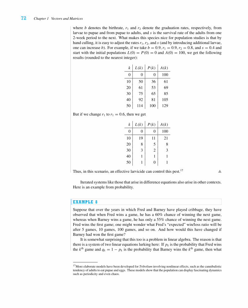
72 Chapter 1 Vectors and Matrices
where b denotes the birthrate, r1 and r2 denote the graduation rates, respectively, fromlarvae to pupae and from pupae to adults, and s is the survival rate of the adults from one2-week period to the next. What makes this species nice for population studies is that byhand culling, it is easy to adjust the rates r1, r2, and s (and by introducing additional larvae,one can increase b). For example, if we take b = 0.9, r1 = 0.9, r2 = 0.8, and s = 0.4 andstart with the initial populations L(0) = P(0) = 0 and A(0) = 100, we get the followingresults (rounded to the nearest integer):
k L(k) P (k) A(k)
0 0 0 100
10 50 36 61
20 61 53 69
30 75 65 85
40 92 81 105
50 114 100 129
But if we change r1 to r1 = 0.6, then we get
k L(k) P (k) A(k)
0 0 0 100
10 19 11 21
20 8 5 8
30 3 2 3
40 1 1 1
50 1 0 1
Thus, in this scenario, an effective larvicide can control this pest.17
Iterated systems like those that arise in difference equations also arise in other contexts.Here is an example from probability.
EXAMPLE 8
Suppose that over the years in which Fred and Barney have played cribbage, they haveobserved that when Fred wins a game, he has a 60% chance of winning the next game,whereas when Barney wins a game, he has only a 55% chance of winning the next game.Fred wins the first game; one might wonder what Fred’s “expected” win/loss ratio will beafter 5 games, 10 games, 100 games, and so on. And how would this have changed ifBarney had won the first game?
It is somewhat surprising that this too is a problem in linear algebra. The reason is thatthere is a system of two linear equations lurking here: If pk is the probability that Fred winsthe kth game and qk = 1 − pk is the probability that Barney wins the kth game, then what
17More elaborate models have been developed for Tribolium involving nonlinear effects, such as the cannibalistictendency of adults to eat pupae and eggs. These models show that the population can display fascinating dynamicssuch as periodicity and even chaos.
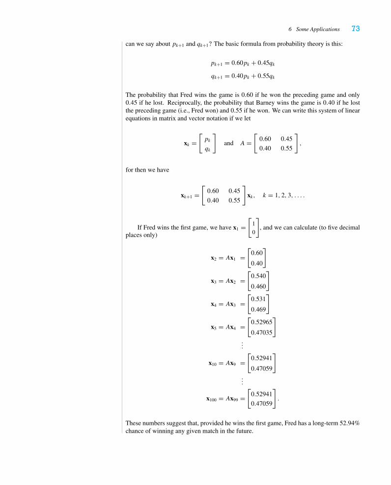
6 Some Applications 73
can we say about pk+1 and qk+1? The basic formula from probability theory is this:
pk+1 = 0.60pk + 0.45qk
qk+1 = 0.40pk + 0.55qk
The probability that Fred wins the game is 0.60 if he won the preceding game and only0.45 if he lost. Reciprocally, the probability that Barney wins the game is 0.40 if he lostthe preceding game (i.e., Fred won) and 0.55 if he won. We can write this system of linearequations in matrix and vector notation if we let
xk =[pk
qk
]and A =
[0.60 0.45
0.40 0.55
],
for then we have
xk+1 =[
0.60 0.45
0.40 0.55
]xk, k = 1, 2, 3, . . . .
If Fred wins the first game, we have x1 =[
1
0
], and we can calculate (to five decimal
places only)
x2 = Ax1 =[
0.60
0.40
]
x3 = Ax2 =[
0.540
0.460
]
x4 = Ax3 =[
0.531
0.469
]
x5 = Ax4 =[
0.52965
0.47035
]
...
x10 = Ax9 =[
0.52941
0.47059
]
...
x100 = Ax99 =[
0.52941
0.47059
].
These numbers suggest that, provided he wins the first game, Fred has a long-term 52.94%chance of winning any given match in the future.
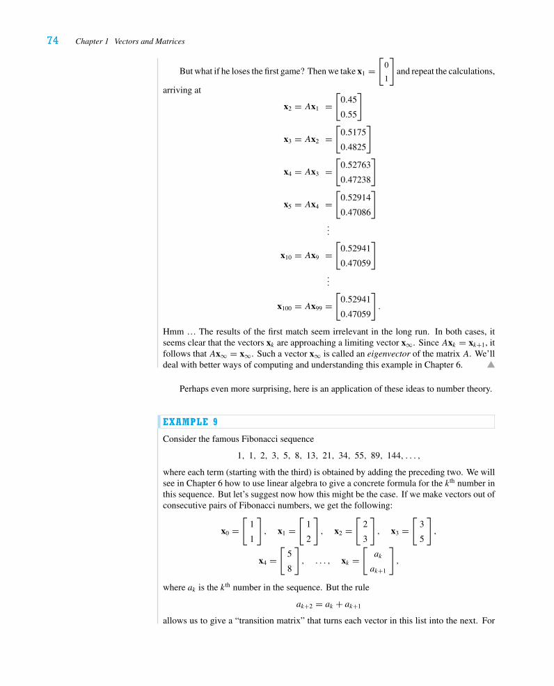
74 Chapter 1 Vectors and Matrices
But what if he loses the first game? Then we take x1 =[
0
1
]and repeat the calculations,
arriving at
x2 = Ax1 =[
0.45
0.55
]
x3 = Ax2 =[
0.5175
0.4825
]
x4 = Ax3 =[
0.52763
0.47238
]
x5 = Ax4 =[
0.52914
0.47086
]
...
x10 = Ax9 =[
0.52941
0.47059
]
...
x100 = Ax99 =[
0.52941
0.47059
].
Hmm … The results of the first match seem irrelevant in the long run. In both cases, itseems clear that the vectors xk are approaching a limiting vector x∞. Since Axk = xk+1, itfollows that Ax∞ = x∞. Such a vector x∞ is called an eigenvector of the matrix A. We’lldeal with better ways of computing and understanding this example in Chapter 6.
Perhaps even more surprising, here is an application of these ideas to number theory.
EXAMPLE 9
Consider the famous Fibonacci sequence
1, 1, 2, 3, 5, 8, 13, 21, 34, 55, 89, 144, . . . ,
where each term (starting with the third) is obtained by adding the preceding two. We willsee in Chapter 6 how to use linear algebra to give a concrete formula for the kth number inthis sequence. But let’s suggest now how this might be the case. If we make vectors out ofconsecutive pairs of Fibonacci numbers, we get the following:
x0 =[
1
1
], x1 =
[1
2
], x2 =
[2
3
], x3 =
[3
5
],
x4 =[
5
8
], . . . , xk =
[ak
ak+1
],
where ak is the kth number in the sequence. But the rule
ak+2 = ak + ak+1
allows us to give a “transition matrix” that turns each vector in this list into the next. For
6 Some Applications 75
example,
x3 =[
3
5
]=[
3
2 + 3
]=[
0 1
1 1
][2
3
]=[
0 1
1 1
]x2;
x4 =[
5
8
]=[
5
3 + 5
]=[
0 1
1 1
][3
5
]=[
0 1
1 1
]x3,
and so on. Since
xk+1 =[ak+1
ak+2
]=[
ak+1
ak + ak+1
]=[
0 1
1 1
][ak
ak+1
]=[
0 1
1 1
]xk,
we see that, as in the previous examples, by repeatedly multiplying our original vector by
the transition matrix
[0 1
1 1
], we can get as far as we’d like in the sequence.
Exercises 1.6
1.∗ (from Henry Burchard Fine’s A College Algebra, 1905) A and B are alloys of silver andcopper. An alloy that is 5 parts A and 3 parts B is 52% silver. One that is 5 parts A and11 parts B is 42% silver. What are the percentages of silver in A and B, respectively?
2. (from Henry Burchard Fine’s A College Algebra, 1905) Two vessels, A and B, containmixtures of alcohol and water. A mixture of 3 parts from A and 2 parts from B willcontain 40% of alcohol; and a mixture of 1 part from A and 2 parts from B will contain32% of alcohol. What are the percentages of alcohol in A and B, respectively?
3. (from Henry Burchard Fine’s A College Algebra, 1905) Two points move at constantrates along the circumference of a circle whose length is 150 ft. When they move inopposite senses they meet every 5 seconds; when they move in the same sense they aretogether every 25 seconds. What are their rates?
4. A grocer mixes dark roast and light roast coffee beans to sell what she calls a Frenchblend and a Viennese blend. For French blend she uses a mixture that is 3 parts darkand 1 part light roast; for Viennese, she uses a mixture that is 1 part dark and 1 partlight roast. If she has at hand 20 pounds of dark roast and 17 pounds of light roast, howmany pounds each of French and Viennese blend can she make so as to have no waste?
5.∗ Find the parabola y = ax2 + bx + c passing through the points (−1, 9), (1,−1), and(2, 3).
6. Find the parabola y = ax2 + bx + c passing through the points (−2,−6), (1, 6), and(3, 4).
7. Let Pi = (xi, yi) ∈ R2, i = 1, 2, 3. Assume x1, x2, and x3 are distinct (i.e., no two areequal).a. Show that the matrix ⎡
⎢⎢⎣1 x1 x2
1
1 x2 x22
1 x3 x23
⎤⎥⎥⎦
is nonsingular.18
18No confusion intended here: x2i means (xi )2, i.e., the square of the real number xi .
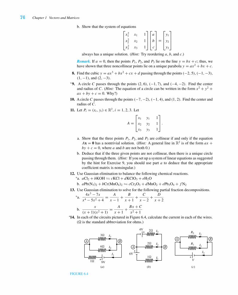
76 Chapter 1 Vectors and Matrices
b. Show that the system of equations⎡⎢⎢⎣x2
1 x1 1
x22 x2 1
x23 x3 1
⎤⎥⎥⎦
⎡⎢⎢⎣a
b
c
⎤⎥⎥⎦ =
⎡⎢⎢⎣y1
y2
y3
⎤⎥⎥⎦
always has a unique solution. (Hint: Try reordering a, b, and c.)
Remark. If a = 0, then the points P1, P2, and P3 lie on the line y = bx + c; thus, wehave shown that three noncollinear points lie on a unique parabola y = ax2 + bx + c.
8. Find the cubic y = ax3 + bx2 + cx + d passing through the points (−2, 5), (−1,−3),(1,−1), and (2,−3).
9.∗ A circle C passes through the points (2, 6), (−1, 7), and (−4,−2). Find the centerand radius of C. (Hint: The equation of a circle can be written in the form x2 + y2 +ax + by + c = 0. Why?)
10. A circle C passes through the points (−7,−2), (−1, 4), and (1, 2). Find the center andradius of C.
11. Let Pi = (xi, yi) ∈ R2, i = 1, 2, 3. Let
A =⎡⎢⎣x1 y1 1
x2 y2 1
x3 y3 1
⎤⎥⎦ .
a. Show that the three points P1, P2, and P3 are collinear if and only if the equationAx = 0 has a nontrivial solution. (Hint: A general line in R2 is of the form ax +by + c = 0, where a and b are not both 0.)
b. Deduce that if the three given points are not collinear, then there is a unique circlepassing through them. (Hint: If you set up a system of linear equations as suggestedby the hint for Exercise 9, you should use part a to deduce that the appropriatecoefficient matrix is nonsingular.)
12. Use Gaussian elimination to balance the following chemical reactions.a.∗ aCl2 + bKOH � cKCl + dKClO3 + eH2O
b. aPb(N3)2 + bCr(MnO4)2 � cCr2O3 + dMnO2 + ePb3O4 + fN2
13. Use Gaussian elimination to solve for the following partial fraction decompositions.
a.∗ 4x3 − 7x
x4 − 5x2 + 4= A
x − 1+ B
x + 1+ C
x − 2+ D
x + 2
b.x
(x + 1)(x2 + 1)= A
x + 1+ Bx + Cx2 + 1
14.∗ In each of the circuits pictured in Figure 6.4, calculate the current in each of the wires.(� is the standard abbreviation for ohms.)
(a) (b) (c)
+ V+
+
+
6V
9V
4VI2
I3
I1
R2
R1
1�
6�
1�
2�
2�
3�
I1I1
I2
I3
I2
I3
A B
A B
A B
FIGURE 6.4
Historical Notes 77
15. Let A be the matrix given in Example 8.a. Show that we can find vectors x ∈ R2 satisfying Ax = x by solving Bx = 0, where
B =[−0.40 0.45
0.40 −0.45
].
(See Exercise 1.4.5.) Give the general solution of Bx = 0 in standard form.
b. Find the solution x of Bx = 0 with x1 + x2 = 1. (Note that in our discussion ofExample 8, we always had pk + qk = 1.)
c. Compare your answer to part b with the vector x∞ obtained in Example 8.
16. Investigate (with a computer or programmable calculator) the cat/mouse populationbehavior in Example 6, choosing a variety of beginning populations, if
a. ck+1 = 0.7ck + 0.1mk
mk+1 = −0.2ck + mk
b.∗ ck+1 = 1.3ck + 0.2mk
mk+1 = −0.1ck + mk
c. ck+1 = 1.1ck + 0.3mk
mk+1 = 0.1ck + 0.9mk
17. Suppose a living organism that can live to a maximum age of 3 years has Leslie matrix
A =
⎡⎢⎢⎣
0 0 812 0 0
0 14 0
⎤⎥⎥⎦ .
Find a stable age distribution vector x, i.e., a vector x ∈ R3 with Ax = x.
18. In Example 9, we took our initial vector to be x0 =[
1
1
].
a. Find the first ten terms of the sequence obtained by starting instead with x′0 =
[2
1
].
b. Describe the sequence obtained by starting instead with x′0 =
[b
c
]. (Hint: Use the
fact that
[b
c
]= b
[1
0
]+ c
[0
1
].)
19. (A computer or calculator may be helpful in solving this problem.) Find numbers a, b,c, d , e, and f so that the five points (0, 2), (−3, 0), (1, 5), (1, 1), and (−1, 1) all lie onthe conic
ax2 + bxy + cy2 + dx + ey + f = 0.
Show, moreover, that a, b, c, d, e, and f are uniquely determined up to a commonfactor.
HISTORICAL NOTESIn writing this text, we have tried to present the material in a logical manner that builds onideas in a fairly linear fashion. Of course, the historical development of the subject didnot go so smoothly. As with any area of mathematics, the ideas and concepts we presentin this text were conceived in fits and starts by many different people, at different times,and for entirely different reasons. Only with hindsight were people able to notice patternsand common threads among earlier developments, and gradually a deeper understandingdeveloped. Some computational elements of linear algebra can be traced to civilizations
78 Chapter 1 Vectors and Matrices
that existed several millennia ago. Throughout history, systems of linear equations havearisen repeatedly in applications. However, the approach we take in today’s linear algebracourse began to develop in the seventeenth century and did not achieve its polished stateuntil the middle of the twentieth. In these historical notes at the end of each chapter, we willmention some of the mathematicians and scientists who played key roles in the developmentof linear algebra, and we will outline a few of the routes taken in that development.
The two central topics of this first chapter are vectors and systems of linear equations.The idea of vector, that of a quantity possessing both magnitude and direction, arose inthe study of mechanics and forces. Sir Isaac Newton (1642–1727) is credited with theformulation of our current view of forces in his work Principia (1687). Pierre de Fermat(1601–1665) and René Descartes (1596–1650) had already laid the groundwork for analyticgeometry. Although Fermat published very little of the mathematics he developed, heis generally given credit for having simultaneously developed the ideas that Descartespublished in La Géométrie (1637).
Following Newton, many scholars began to use directed line segments to representforces and the parallelogram rule to add such segments. Joseph-Louis Lagrange (1736–1813) published his Mécanique analytique in 1788, in which he summarized all the post-Newtonian efforts in a single cohesive mathematical treatise on forces and mechanics.Later, another French mathematician, Louis Poinsot (1777–1859), took the geometry ofvector forces to yet another level in his Éléments de statique and his subsequent work, inwhich he invented the geometric study of statics.
Some of these ideas, however, had first appeared 2000 years before Newton. In Physics,Aristotle (384–322 BCE) essentially introduced the notion of vector by discussing a forcein terms of the distance and direction it displaced an object. Aristotle’s work is purelydescriptive and not mathematical. In a later work, Mechanics, often credited toAristotle butnow believed to be the work of scholarly peers, we find the following insightful observation:
Now whenever a body is moved in two directions in a fixed ratio, it necessarilytravels in a straight line, which is the diagonal of the figure which the linesarranged in this ratio describe.
This is, of course, the parallelogram rule.As for systems of linear equations, virtually all historians cite a particular excerpt from
the Nine Chapters of the Mathematical Art as the earliest use of what would come to be themodern method for solving such systems, elimination. This text, written during the years200–100 BCE, at the beginning of the intellectually fruitful Han dynasty, represents thestate of Chinese mathematics at that time.
There are three types of corn. One bundle of the first type, two of the second, andthree of the third total to 26 measures. Two bundles of the first type, three of thesecond, and one of the third total 34 measures. Lastly, three bundles of corn of thefirst type, two bundles of the second type, and one bundle of the third type make atotal of 39 measures. How many measures make up a single bundle of each type?
Yes, even back then they had the dreaded word problem!Today, we would solve this problem by letting x, y, and z represent the measures in
a single bundle of each type of corn, translating the word problem to the system of linearequations
x + 2y + 3z = 26
2x + 3y + z = 34
3x + 2y + z = 39 .
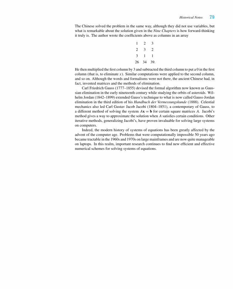
Historical Notes 79
The Chinese solved the problem in the same way, although they did not use variables, butwhat is remarkable about the solution given in the Nine Chapters is how forward-thinkingit truly is. The author wrote the coefficients above as columns in an array
1 2 3
2 3 2
3 1 1
26 34 39.
He then multiplied the first column by 3 and subtracted the third column to put a 0 in the firstcolumn (that is, to eliminate x). Similar computations were applied to the second column,and so on. Although the words and formalisms were not there, the ancient Chinese had, infact, invented matrices and the methods of elimination.
Carl Friedrich Gauss (1777–1855) devised the formal algorithm now known as Gaus-sian elimination in the early nineteenth century while studying the orbits of asteroids. Wil-helm Jordan (1842–1899) extended Gauss’s technique to what is now called Gauss-Jordanelimination in the third edition of his Handbuch der Vermessungskunde (1888). Celestialmechanics also led Carl Gustav Jacob Jacobi (1804–1851), a contemporary of Gauss, toa different method of solving the system Ax = b for certain square matrices A. Jacobi’smethod gives a way to approximate the solution when A satisfies certain conditions. Otheriterative methods, generalizing Jacobi’s, have proven invaluable for solving large systemson computers.
Indeed, the modern history of systems of equations has been greatly affected by theadvent of the computer age. Problems that were computationally impossible 50 years agobecame tractable in the 1960s and 1970s on large mainframes and are now quite manageableon laptops. In this realm, important research continues to find new efficient and effectivenumerical schemes for solving systems of equations.

This page intentionally left blank
81
C H A P T E R 2MATRIX ALGEBRA
I n the previous chapter we introduced matrices as a shorthand device for representingsystems of linear equations. Now we will see that matrices have a life of their own, first
algebraically and then geometrically. The crucial new ingredient is to interpret an m× nmatrix as a special sort of function that assigns to each vector x ∈ Rn the productAx ∈ Rm.
1 Matrix Operations
Recall that an m× n matrix A is a rectangular array of mn real numbers,
A =
⎡⎢⎢⎢⎢⎢⎣
a11 . . . a1n
a21 . . . a2n
.... . .
...
am1 . . . amn
⎤⎥⎥⎥⎥⎥⎦,
where aij represents the entry in the i th row and j th column. We recall that two m× nmatrices A and B are equal if aij = bij for all i = 1, . . . , m and j = 1, . . . , n.
We take this opportunity to warn our readers that the word if is ordinarily used inmathematical definitions, even though it should be the phrase if and only if . That is,even though we don’t say so, we intend it to be understood that, for example, in thiscase, if A = B, then aij = bij for all i and j . Be warned: This custom applies onlyto definitions, not to propositions and theorems! See the earlier discussions of if andonly if on p. 21.
A has m row vectors,
A1 = (a11, . . . , a1n),
A2 = (a21, . . . , a2n),
...
Am = (am1, . . . , amn),
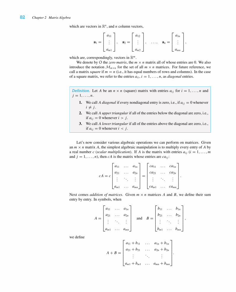
82 Chapter 2 Matrix Algebra
which are vectors in Rn, and n column vectors,
a1 =
⎡⎢⎢⎣a11
...
am1
⎤⎥⎥⎦ , a2 =
⎡⎢⎢⎣a12
...
am2
⎤⎥⎥⎦ , . . . , an =
⎡⎢⎢⎣a1n
...
amn
⎤⎥⎥⎦ ,
which are, correspondingly, vectors in Rm.We denote by O the zero matrix, the m× n matrix all of whose entries are 0. We also
introduce the notation Mm×n for the set of all m× n matrices. For future reference, wecall a matrix square if m = n (i.e., it has equal numbers of rows and columns). In the caseof a square matrix, we refer to the entries aii , i = 1, . . . , n, as diagonal entries.
Definition. Let A be an n× n (square) matrix with entries aij for i = 1, . . . , n andj = 1, . . . , n.
1. We callA diagonal if every nondiagonal entry is zero, i.e., if aij = 0 wheneveri �= j .
2. We callA upper triangular if all of the entries below the diagonal are zero, i.e.,if aij = 0 whenever i > j .
3. We callA lower triangular if all of the entries above the diagonal are zero, i.e.,if aij = 0 whenever i < j .
Let’s now consider various algebraic operations we can perform on matrices. Givenan m× n matrix A, the simplest algebraic manipulation is to multiply every entry of A bya real number c (scalar multiplication). If A is the matrix with entries aij (i = 1, . . . , mand j = 1, . . . , n), then cA is the matrix whose entries are caij :
cA = c
⎡⎢⎢⎢⎢⎢⎣
a11 . . . a1n
a21 . . . a2n
.... . .
...
am1 . . . amn
⎤⎥⎥⎥⎥⎥⎦
=
⎡⎢⎢⎢⎢⎢⎣
ca11 . . . ca1n
ca21 . . . ca2n
.... . .
...
cam1 . . . camn
⎤⎥⎥⎥⎥⎥⎦.
Next comes addition of matrices. Given m× n matrices A and B, we define their sumentry by entry. In symbols, when
A =
⎡⎢⎢⎢⎢⎢⎣
a11 . . . a1n
a21 . . . a2n
.... . .
...
am1 . . . amn
⎤⎥⎥⎥⎥⎥⎦
and B =
⎡⎢⎢⎢⎢⎢⎣
b11 . . . b1n
b21 . . . b2n
.... . .
...
bm1 . . . bmn
⎤⎥⎥⎥⎥⎥⎦,
we define
A+ B =
⎡⎢⎢⎢⎢⎢⎣
a11 + b11 . . . a1n + b1n
a21 + b21 . . . a2n + b2n
.... . .
...
am1 + bm1 . . . amn + bmn
⎤⎥⎥⎥⎥⎥⎦.
1 Matrix Operations 83
It is important to understand that when we refer to the set of allm× nmatrices, Mm×n,we have not specified the positive integers m and n. They can be chosen arbitrarily.However, when we say thatA,B ∈ Mm×n, we mean thatA andB must have the same“shape,” i.e., the same number of rows (m) and the same number of columns (n).
EXAMPLE 1
Let c = −2 and
A =
⎡⎢⎢⎣
1 2 3
2 1 −2
4 −1 3
⎤⎥⎥⎦ , B =
⎡⎢⎢⎣
6 4 −1
−3 1 1
0 0 0
⎤⎥⎥⎦ , C =
[1 2 1
2 1 1
].
Then
cA =
⎡⎢⎢⎣
−2 −4 −6
−4 −2 4
−8 2 −6
⎤⎥⎥⎦ , A+ B =
⎡⎢⎢⎣
7 6 2
−1 2 −1
4 −1 3
⎤⎥⎥⎦ ,
and neither sum A+ C nor B + C makes sense, because C has a different shape from A
and B.
We leave it to the reader to check that scalar multiplication of matrices and matrix ad-dition satisfy the same list of properties we gave in Exercise 1.1.28 for scalar multiplicationof vectors and vector addition. We list them here for reference.
Proposition 1.1. Let A,B,C ∈ Mm×n and let c, d ∈ R.
1. A+ B = B + A.
2. (A+ B)+ C = A+ (B + C).3. O + A = A.
4. There is a matrix −A so that A+ (−A) = O.
5. c(dA) = (cd)A.
6. c(A+ B) = cA+ cB.
7. (c + d)A = cA+ dA.
8. 1A = A.
Proof. Left to the reader in Exercise 3.
To understand these properties, one might simply examine corresponding entries ofthe appropriate matrices and use the relevant properties of real numbers to see whythey are equal. A more elegant approach is the following: We can encode an m× nmatrix as a vector in Rmn, for example,
⎡⎢⎢⎣
1 −1
2 3
−5 4
⎤⎥⎥⎦ ∈ M3×2 � (1,−1, 2, 3,−5, 4) ∈ R6,
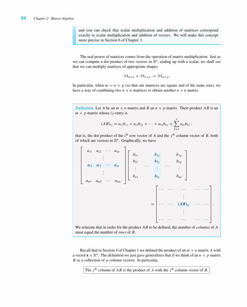
84 Chapter 2 Matrix Algebra
and you can check that scalar multiplication and addition of matrices correspondexactly to scalar multiplication and addition of vectors. We will make this conceptmore precise in Section 6 of Chapter 3.
The real power of matrices comes from the operation of matrix multiplication. Just aswe can compute a dot product of two vectors in Rn, ending up with a scalar, we shall seethat we can multiply matrices of appropriate shapes:
Mm×n × Mn×p → Mm×p.
In particular, when m = n = p (so that our matrices are square and of the same size), wehave a way of combining two n× n matrices to obtain another n× n matrix.
Definition. Let A be an m× n matrix and B an n× p matrix. Their product AB is anm× p matrix whose ij -entry is
(AB)ij = ai1b1j + ai2b2j + · · · + ainbnj =n∑k=1
aikbkj ;
that is, the dot product of the i th row vector of A and the j th column vector of B, bothof which are vectors in Rn. Graphically, we have⎡⎢⎢⎢⎢⎢⎢⎢⎢⎢⎣
a11 a12 · · · a1n
...
ai1 ai2 · · · ain
...
am1 am2 · · · amn
⎤⎥⎥⎥⎥⎥⎥⎥⎥⎥⎦
⎡⎢⎢⎢⎢⎢⎢⎣
b11
b21
...
bn1
. . .
b1j
b2j
...
bnj
. . .
b1p
b2p
...
bnp
⎤⎥⎥⎥⎥⎥⎥⎦
=
⎡⎢⎢⎢⎢⎢⎢⎢⎢⎢⎣
· · · · · · · · · · · · · · ·...
· · · · · · (AB)ij · · · · · ·...
· · · · · · · · · · · · · · ·
⎤⎥⎥⎥⎥⎥⎥⎥⎥⎥⎦
.
We reiterate that in order for the product AB to be defined, the number of columns of Amust equal the number of rows of B.
Recall that in Section 4 of Chapter 1 we defined the product of anm× nmatrixAwitha vector x ∈ Rn. The definition we just gave generalizes that if we think of an n× p matrixB as a collection of p column vectors. In particular,
The j th column of AB is the product of A with the j th column vector of B.
1 Matrix Operations 85
EXAMPLE 2
Note that this definition is compatible with our definition in Chapter 1 of the multiplicationof an m× n matrix with a column vector in Rn (an n× 1 matrix). For example, if
A =
⎡⎢⎢⎣
1 3
2 −1
1 1
⎤⎥⎥⎦ , x =
[4
−1
], and B =
[4 1 0 −2
−1 1 5 1
],
then
Ax =
⎡⎢⎢⎣
1 3
2 −1
1 1
⎤⎥⎥⎦
⎡⎣ 4
−1
⎤⎦ =
⎡⎢⎢⎢⎣
1
9
3
⎤⎥⎥⎥⎦ , and
AB =
⎡⎢⎢⎣
1 3
2 −1
1 1
⎤⎥⎥⎦
⎡⎣ 4
−1
1
1
0
5
−2
1
⎤⎦ =
⎡⎢⎢⎢⎣
1
9
3
4
1
2
15
−5
5
1
−5
−1
⎤⎥⎥⎥⎦ .
Notice also that the product BA does not make sense: B is a 2 × 4 matrix and A is 3 × 2,and 4 �= 3.
The preceding example brings out an important point about the nature of matrix mul-tiplication: It can happen that the matrix product AB is defined and the product BA is not.Now if A is an m× n matrix and B is an n×m matrix, then both products AB and BAmake sense: AB is m×m and BA is n× n. Notice that these are both square matrices,but of different sizes.
EXAMPLE 3
To see an extreme example of this, consider the 1 × 3 matrix A =[1 2 3
]and the
3 × 1 matrix B =
⎡⎢⎢⎣
1
−1
2
⎤⎥⎥⎦. Then
AB =[1 2 3
]⎡⎢⎢⎣
1
−1
2
⎤⎥⎥⎦ =
[5], whereas
BA =
⎡⎢⎢⎣
1
−1
2
⎤⎥⎥⎦[1 2 3
]=
⎡⎢⎢⎣
1 2 3
−1 −2 −3
2 4 6
⎤⎥⎥⎦ .
Even if we start with both A and B as n× n matrices, the products AB and BA havethe same shape but need not be equal.
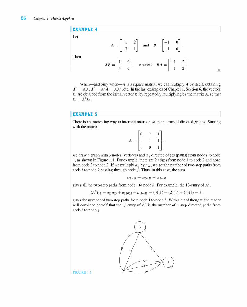
86 Chapter 2 Matrix Algebra
EXAMPLE 4
Let
A =[
1 2
−3 1
]and B =
[−1 0
1 0
].
Then
AB =[
1 0
4 0
], whereas BA =
[−1 −2
1 2
].
When—and only when—A is a square matrix, we can multiply A by itself, obtainingA2 = AA,A3 = A2A = AA2, etc. In the last examples of Chapter 1, Section 6, the vectorsxk are obtained from the initial vector x0 by repeatedly multiplying by the matrix A, so thatxk = Akx0.
EXAMPLE 5
There is an interesting way to interpret matrix powers in terms of directed graphs. Startingwith the matrix
A =
⎡⎢⎢⎣
0 2 1
1 1 1
1 0 1
⎤⎥⎥⎦ ,
we draw a graph with 3 nodes (vertices) and aij directed edges (paths) from node i to nodej , as shown in Figure 1.1. For example, there are 2 edges from node 1 to node 2 and nonefrom node 3 to node 2. If we multiply aij by ajk , we get the number of two-step paths fromnode i to node k passing through node j . Thus, in this case, the sum
ai1a1k + ai2a2k + ai3a3k
gives all the two-step paths from node i to node k. For example, the 13-entry of A2,
(A2)13 = a11a13 + a12a23 + a13a33 = (0)(1)+ (2)(1)+ (1)(1) = 3,
gives the number of two-step paths from node 1 to node 3. With a bit of thought, the readerwill convince herself that the ij -entry of An is the number of n-step directed paths fromnode i to node j .
FIGURE 1.1 1
2
3
1 Matrix Operations 87
We calculate
A2 =
⎡⎢⎢⎣
0 2 1
1 1 1
1 0 1
⎤⎥⎥⎦
⎡⎢⎢⎣
0 2 1
1 1 1
1 0 1
⎤⎥⎥⎦ =
⎡⎢⎢⎣
3 2 3
2 3 3
1 2 2
⎤⎥⎥⎦ ,
A3 =
⎡⎢⎢⎣
5 8 8
6 7 8
4 4 5
⎤⎥⎥⎦ , and . . .
A7 =
⎡⎢⎢⎣
272 338 377
273 337 377
169 208 233
⎤⎥⎥⎦ .
In particular, there are 169 seven-step paths from node 3 to node 1.
We have seen that, in general, matrix multiplication is not commutative. However, itdoes have the following crucial properties. Let In denote the n× n matrix with 1’s on thediagonal and 0’s elsewhere, as illustrated on p. 61.
Proposition 1.2. Let A and A′ be m× n matrices, let B and B ′ be n× p matrices, let Cbe a p × q matrix, and let c be a scalar. Then
1. AIn = A = ImA. For this reason, In is called the n× n identity matrix.
2. (A+ A′)B = AB + A′B and A(B + B ′) = AB + AB ′. This is the distributiveproperty of matrix multiplication over matrix addition.
3. (cA)B = c(AB) = A(cB).
4. (AB)C = A(BC). This is the associative property of matrix multiplication.
Proof. We prove the associative property and leave the rest to the reader in Exercise 4.Note first of all that there is hope: AB is an m× p matrix and C is a p × q matrix, so(AB)C will be anm× q matrix; similarly, A is anm× nmatrix and BC is a n× q matrix,so A(BC) will be an m× q matrix. Associativity amounts to the statement that
(AB)c = A(Bc)
for any column vector c of the matrixC: To calculate the j th column of (AB)C we multiplyAB by the j th column of C; to calculate the j th column of A(BC) we multiply A by the j th
column of BC, which, in turn, is the product of B with the j th column of C.Letting b1, . . . ,bp denote the column vectors of B, we recall (see the crucial observa-
tion (∗) on p. 53) thatBc is the linear combination c1b1 + c2b2 + · · · + cpbp, and so (usingProposition 5.2 of Chapter 1)
A(Bc) =A(c1b1 + c2b2 + · · · + cpbp) = c1(Ab1)+ c2(Ab2)+ · · · + cp(Abp)
= c1(first column of AB)+ c2(second column of AB)
+ · · · + cp(pth column of AB)
= (AB)c.There is an important conceptual point underlying this computation, as we now study.
Through Chapter 1, we thought of matrices simply as an algebraic shorthand for deal-ing with systems of linear equations. However, we can interpret matrices as functions,
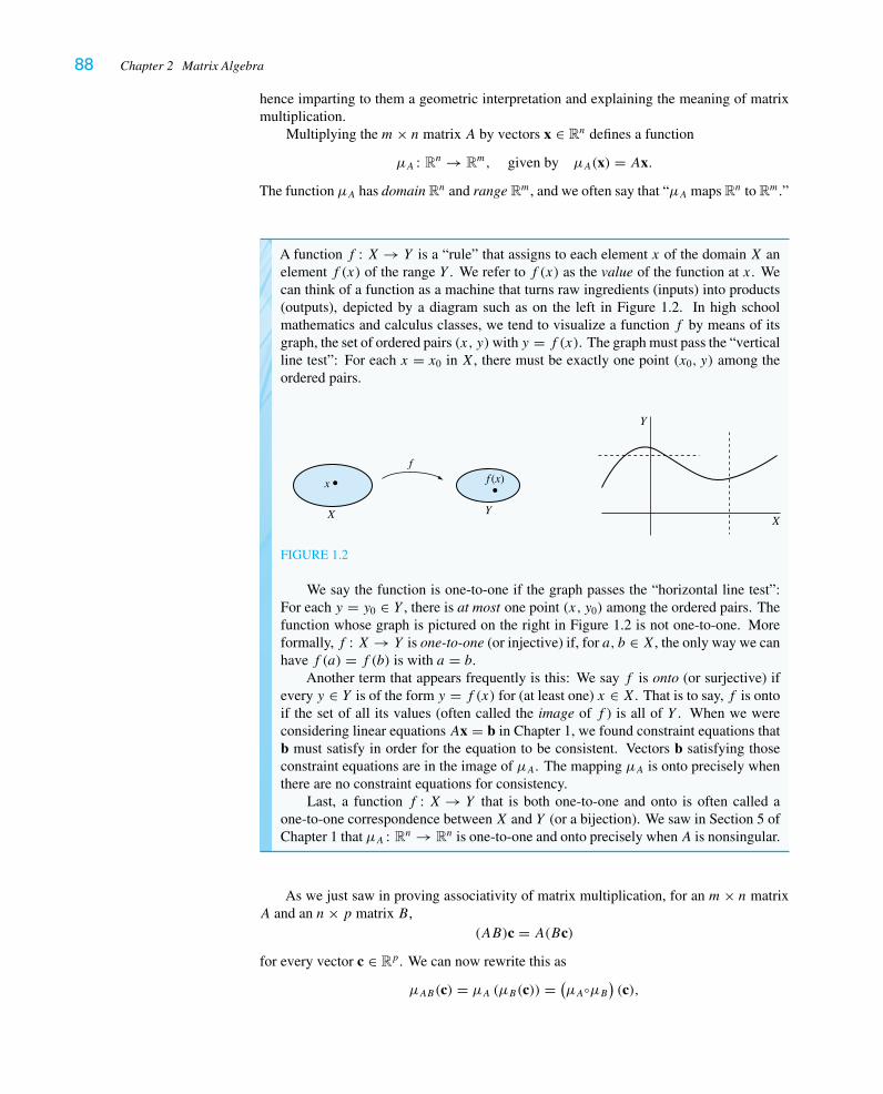
88 Chapter 2 Matrix Algebra
hence imparting to them a geometric interpretation and explaining the meaning of matrixmultiplication.
Multiplying the m× n matrix A by vectors x ∈ Rn defines a function
μA : Rn → Rm, given by μA(x) = Ax.
The function μA has domain Rn and range Rm, and we often say that “μA maps Rn to Rm.”
A function f : X → Y is a “rule” that assigns to each element x of the domain X anelement f (x) of the range Y . We refer to f (x) as the value of the function at x. Wecan think of a function as a machine that turns raw ingredients (inputs) into products(outputs), depicted by a diagram such as on the left in Figure 1.2. In high schoolmathematics and calculus classes, we tend to visualize a function f by means of itsgraph, the set of ordered pairs (x, y)with y = f (x). The graph must pass the “verticalline test”: For each x = x0 in X, there must be exactly one point (x0, y) among theordered pairs.
X
x
f
Y
Y
X
f (x)
FIGURE 1.2
We say the function is one-to-one if the graph passes the “horizontal line test”:For each y = y0 ∈ Y , there is at most one point (x, y0) among the ordered pairs. Thefunction whose graph is pictured on the right in Figure 1.2 is not one-to-one. Moreformally, f : X → Y is one-to-one (or injective) if, for a, b ∈ X, the only way we canhave f (a) = f (b) is with a = b.
Another term that appears frequently is this: We say f is onto (or surjective) ifevery y ∈ Y is of the form y = f (x) for (at least one) x ∈ X. That is to say, f is ontoif the set of all its values (often called the image of f ) is all of Y . When we wereconsidering linear equations Ax = b in Chapter 1, we found constraint equations thatb must satisfy in order for the equation to be consistent. Vectors b satisfying thoseconstraint equations are in the image of μA. The mapping μA is onto precisely whenthere are no constraint equations for consistency.
Last, a function f : X → Y that is both one-to-one and onto is often called aone-to-one correspondence between X and Y (or a bijection). We saw in Section 5 ofChapter 1 that μA : Rn → Rn is one-to-one and onto precisely whenA is nonsingular.
As we just saw in proving associativity of matrix multiplication, for an m× n matrixA and an n× p matrix B,
(AB)c = A(Bc)
for every vector c ∈ Rp. We can now rewrite this as
μAB(c) = μA (μB(c)) = (μA◦μB)(c),
1 Matrix Operations 89
where the latter notation denotes composition of functions. Of course, this formula is the realmotivation for defining matrix multiplication as we did. In fact, one might define the matrixproduct as a composition of functions and then derive the computational formula. Now, weknow that composition of functions is associative (even though it is not commutative):
(f ◦g)◦h = f ◦(g◦h),
from which we infer that(μA◦μB
)◦μC = μA◦
(μB◦μC
), and so
μ(AB)C = μA(BC); that is,
(AB)C = A(BC).
This is how one should understand matrix multiplication and its associativity.
Remark. Mathematicians will often express the rule μAB = μA◦μB schematically by thefollowing diagram:
μAB
μB μAR
pR
nR
m
We will continue to explore the interpretation of matrices as functions in the next section.
Exercises 2.1
1. Let A =[
1 2
3 4
], B =
[2 1
4 3
], C =
[1 2 1
0 1 2
], and D =
⎡⎢⎣
0 1
1 0
2 3
⎤⎥⎦. Calculate each
of the following expressions or explain why it is not defined.a. A+ Bb.∗ 2A− Bc. A− C
d. C +De. AB
f.∗ BA
g.∗ AC
h.∗ CA
i. BD
j. DB
k.∗ CD
l.∗ DC
2. LetA =[
1 1
2 2
]and B =
[−1 3
1 −3
]. Show thatAB = O but BA �= O. Explain this
result geometrically.
3. Prove Proposition 1.1. While you’re at it, prove (using these properties) that for anyA ∈ Mm×n, 0A = O.
4. a. Prove the remainder of Proposition 1.2.
b. Interpret parts 1, 2, and 3 of Proposition 1.2 in terms of properties of functions.
c. Suppose Charlie has carefully proved the first statement in part 2 and offers thefollowing justification of the second: Since (B + B ′)A = BA+ B ′A, we nowhaveA(B + B ′) = (B + B ′)A = BA+ B ′A = AB + AB ′ = A(B + B ′). Decidewhether he is correct.
5. a.∗ If A is an m× n matrix and Ax = 0 for all x ∈ Rn, show that A = O.
b. If A and B are m× n matrices and Ax = Bx for all x ∈ Rn, show that A = B.
6. Prove or give a counterexample. Assume all the matrices are n× n.a. If AB = CB and B �= O, then A = C.
b. If A2 = A, then A = O or A = I .
90 Chapter 2 Matrix Algebra
c. (A+ B)(A− B) = A2 − B2.
d. If AB = CB and B is nonsingular, then A = C.
e. If AB = BC and B is nonsingular, then A = C.
In the box on p. 52, we suggested that in such a problem you might try n = 1 to getintuition. Well, if we have real numbers a, b, and c satisfying ab = cb, then ab − cb =(a − c)b = 0, so b = 0 or a = c. Similarly, if a2 = a, then a2 − a = a(a − 1) = 0,so a = 0 or a = 1, and so on. So, once again, it’s not clear that the case n = 1 givesmuch insight into the general case. But it might lead us to the right question: Is it truefor n× n matrices that AB = O implies A = O or B = O?
To answer this question, you might either play around with numerical examples(e.g., with 2 × 2 matrices) or interpret this matrix product geometrically: What doesit say about the relation between the rows of A and the columns of B?
7. Find all 2 × 2 matrices A =[a b
c d
]satisfying
a. A2 = I2 b.∗ A2 = O c. A2 = −I2
8. For each of the following matrices A, find a formula for Ak for positive integers k. (Ifyou know how to do proof by induction, please do.)
a. A =[
2 0
0 3
]b. A =
⎡⎢⎢⎢⎢⎣
d1
d2
. . .
dn
⎤⎥⎥⎥⎥⎦
c. A =[
1 1
0 1
]
9. (Block multiplication) We can think of an (m+ n)× (m+ n) matrix as being decom-posed into “blocks,” and thinking of these blocks as matrices themselves, we can formproducts and sums appropriately. Suppose A and A′ are m×m matrices, B and B ′are m× n matrices, C and C ′ are n×m matrices, and D and D′ are n× n matrices.Verify the following formula for the product of “block” matrices:
[A B
C D
][A′ B ′
C ′ D′
]=[AA′ + BC ′ AB ′ + BD′
CA′ +DC ′ CB ′ +DD′
].
10. Suppose A and B are nonsingular n× n matrices. Prove that AB is nonsingular.
Although it is tempting to try to show that the reduced echelon form ofAB is the identitymatrix, there is no direct way to do this. As is the case in most non-numerical problemsregarding nonsingularity, you should remember thatAB is nonsingular precisely whenthe only solution of (AB)x = 0 is x = 0.
11. a.� SupposeA ∈ Mm×n, B ∈ Mn×m, and BA = In. Prove that if for some b ∈ Rm theequation Ax = b has a solution, then that solution is unique.
b. Suppose A ∈ Mm×n, C ∈ Mn×m, and AC = Im. Prove that the system Ax = b isconsistent for every b ∈ Rm.
2 Linear Transformations: An Introduction 91
To show that if a solution exists, then it is unique, one approach (which works wellhere) is to suppose that x satisfies the equation and find a formula that determinesit. Another approach is to assume that x and y are both solutions and then use theequations to prove that x = y.
To prove that a solution exists, the direct approach (which works here) is to findsome x that works—even if that means guessing. A more subtle approach to existencequestions involves proof by contradiction (see the box on p. 18): Assume there is nosolution, and deduce from this assumption something that is known to be false.
c.� Suppose A ∈ Mm×n and B,C ∈ Mn×m are matrices that satisfy BA = In andAC = Im. Prove that B = C.
12. An n× n matrix is called a permutation matrix if it has a single 1 in each row andcolumn and all its remaining entries are 0.a. Write down all the 2 × 2 permutation matrices. How many are there?
b. Write down all the 3 × 3 permutation matrices. How many are there?
c. Show that the product of two permutation matrices is again a permutation matrix.Do they commute?
d. Prove that every permutation matrix is nonsingular.
e. IfA is an n× nmatrix and P is an n× n permutation matrix, describe the columnsof AP and the rows of PA.
13. Find matrices A so that
a. A �= O, but A2 = O
b. A2 �= O, but A3 = O
Can you make a conjecture about matrices satisfying An−1 �= O but An = O?
14. Find all 2 × 2 matricesA that commute with all 2 × 2 matricesB. That is, ifAB = BA
for all B ∈ M2×2, what are the possible matrices that A can be?
15. (The binomial theorem for matrices) Suppose A and B are n× n matrices with theproperty that AB = BA. Prove that for any positive integer k, we have
(A+ B)k =k∑i=0
k!i!(k − i)!A
k−iBi
= Ak + kAk−1B + k(k − 1)
2Ak−2B2 + k(k − 1)(k − 2)
6Ak−3B3
+ · · · + kABk−1 + Bk.Show that the result is false when AB �= BA.
2 Linear Transformations: An IntroductionThe function μA we defined at the end of Section 1 is a prototype of the functions onestudies in linear algebra, called linear transformations. We shall explore them in greaterdetail in Chapter 4, but here we want to familiarize ourselves with a number of examples.First, a definition:
92 Chapter 2 Matrix Algebra
Definition. A function T : Rn → Rm is called a linear transformation (or linear map)if it satisfies
(i) T (x + y) = T (x)+ T (y) for all x, y ∈ Rn.
(ii) T (cx) = cT (x) for all x ∈ Rn and all scalars c.
These are often called the linearity properties.
EXAMPLE 1
Here are a few examples of functions, some linear, some not.
(a) Consider the function T : R2 → R2 defined by T
([x1
x2
])=[x1 + x2
x1
]. Let’s decide
whether it satisfies the two properties of a linear map.
(i)
T
([x1
x2
]+[y1
y2
])= T
([x1 + y1
x2 + y2
])
=[(x1 + y1)+ (x2 + y2)
(x1 + y1)
]=[(x1 + x2)+ (y1 + y2)
x1 + y1
]
=[x1 + x2
x1
]+[y1 + y2
y1
]= T
([x1
x2
])+ T
([y1
y2
])
(ii)
T
(c
[x1
x2
])= T
([cx1
cx2
])=[cx1 + cx2
cx1
]
= c
[x1 + x2
x1
]= cT
([x1
x2
])for all scalars c.
Thus, T is a linear map.
It is important to remember that we have to check that the equationT (x + y) = T (x)+T (y) holds for all vectors x and y, so the argument must be an algebraic one usingvariables. Similarly, we must show T (cx) = cT (x) for all vectors x and all scalars c.It is not enough to check a few cases.
(b) What about the function T : R2 → R2 defined by T
([x1
x2
])=[x1
2
]? Here we can
see that both properties fail, but we only need to provide evidence that one fails.
For example, T
(3
[1
1
])= T
([3
3
])=[
3
2
]�= 3
[1
2
], which is what 3T
([1
1
])
2 Linear Transformations: An Introduction 93
would be. The reader can also try checking whether
T
([1
1
])= T
([1
0
]+[
0
1
])= T
([1
0
])+ T
([0
1
]).
Just a reminder: To check that a multi-part (in this case, two-part) definition holds,we must check each condition. However, to show that a multi-part definition fails, weonly need to show that one of the criteria does not hold.
(c) We learned in Section 2 of Chapter 1 to project one vector onto another. We nowthink of this as defining a function: Let a ∈ R2 be fixed and let T : R2 → R2 be givenby T (x) = projax. One can give a geometric argument that this is a linear map (seeExercise 15), but we will use our earlier formula from p. 22 to establish this. Since
projax = x · a‖a‖2
a,
we have
(i) T (x + y) = (x + y) · a‖a‖2
a = x · a‖a‖2
a + y · a‖a‖2
a = T (x)+ T (y), and
(ii) T (cx) = (cx) · a‖a‖2
a = cx · a‖a‖2
a = cT (x).
Notice that if we replace a with a nonzero scalar multiple of a, the map T doesn’tchange. For this reason, we will refer to T = proja as the projection of R2 onto theline �, where � is the line spanned by a. We will denote this mapping by P�.
(d) It follows from Exercise 1.4.13 (see also Proposition 5.2 of Chapter 1) that for anym× n matrix A, the function μA : Rn → Rm is a linear transformation.
EXAMPLE 2
Expanding on the previous example, we consider the linear transformations μA : R2 → R2
for some specific 2 × 2 matrices A and give geometric interpretations of these maps.
(a) IfA =[
0 0
0 0
]= O is the zero matrix, thenAx = 0 for all x ∈ R2, soμA sends every
vector in R2 to the zero vector 0. If B =[
1 0
0 1
]= I2 is the 2 × 2 identity matrix,
then Bx = x for all x ∈ R2. The function μB is the identity map from R2 to R2.
(b) Consider the linear transformation T : R2 → R2 defined by multiplication by thematrix
A =[
1 1
0 1
].
The effect of T is pictured in Figure 2.1. One might slide a deck of cards in thisfashion, and such a motion is called a shear.
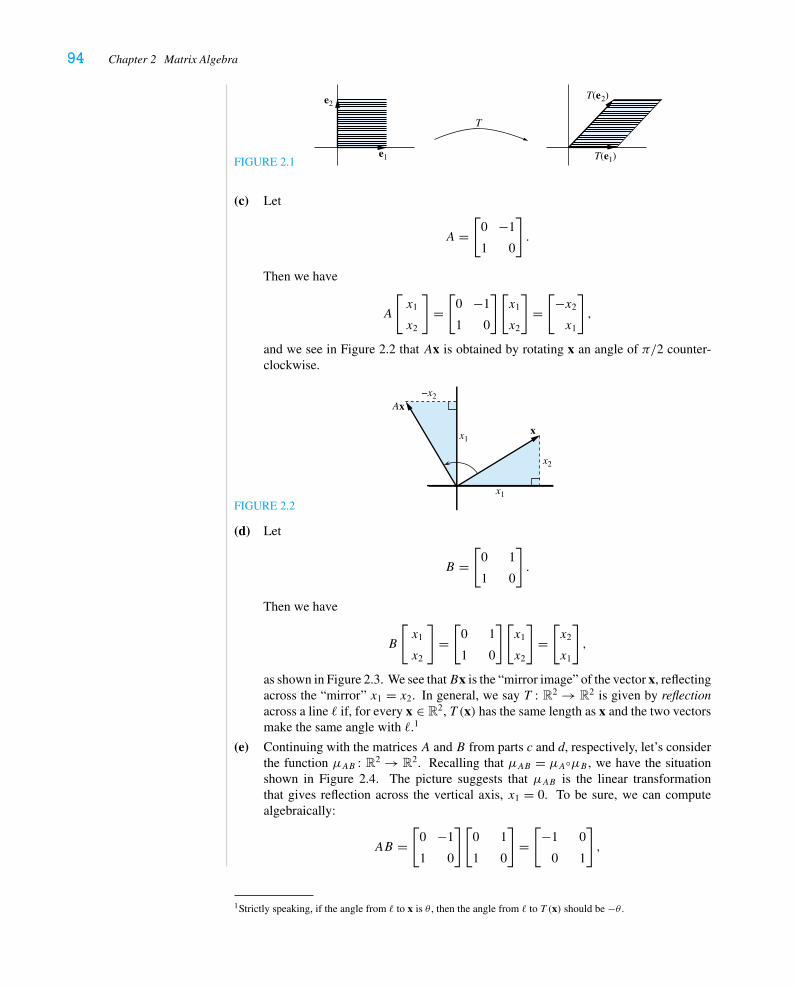
94 Chapter 2 Matrix Algebra
FIGURE 2.1
T
e2
e1 T(e1)
T(e2)
(c) Let
A =[
0 −1
1 0
].
Then we have
A
[x1
x2
]=[
0 −1
1 0
][x1
x2
]=[−x2
x1
],
and we see in Figure 2.2 that Ax is obtained by rotating x an angle of π/2 counter-clockwise.
FIGURE 2.2
x
Ax
x1
x2
−x2
x1
(d) Let
B =[
0 1
1 0
].
Then we have
B
[x1
x2
]=[
0 1
1 0
][x1
x2
]=[x2
x1
],
as shown in Figure 2.3. We see thatBx is the “mirror image” of the vector x, reflectingacross the “mirror” x1 = x2. In general, we say T : R2 → R2 is given by reflectionacross a line � if, for every x ∈ R2, T (x) has the same length as x and the two vectorsmake the same angle with �.1
(e) Continuing with the matrices A and B from parts c and d, respectively, let’s considerthe function μAB : R2 → R2. Recalling that μAB = μA◦μB , we have the situationshown in Figure 2.4. The picture suggests that μAB is the linear transformationthat gives reflection across the vertical axis, x1 = 0. To be sure, we can computealgebraically:
AB =[
0 −1
1 0
][0 1
1 0
]=[−1 0
0 1
],
1Strictly speaking, if the angle from � to x is θ , then the angle from � to T (x) should be −θ .
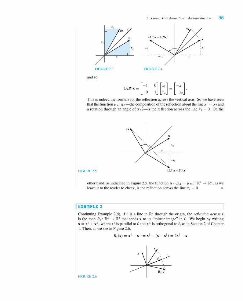
2 Linear Transformations: An Introduction 95
x
x1
x1
x2
x2Bx �
FIGURE 2.3
x
Bx
(AB)x = A(Bx)
x1−x1
x2x2
FIGURE 2.4
and so
(AB)x =[−1 0
0 1
][x1
x2
]=[−x1
x2
].
This is indeed the formula for the reflection across the vertical axis. So we have seenthat the functionμA◦μB—the composition of the reflection about the line x1 = x2 anda rotation through an angle of π/2—is the reflection across the line x1 = 0. On the
FIGURE 2.5
x
Ax
(BA)x = B(Ax)
−x2
x1
x2
other hand, as indicated in Figure 2.5, the function μB◦μA = μBA : R2 → R2, as weleave it to the reader to check, is the reflection across the line x2 = 0.
EXAMPLE 3
Continuing Example 2(d), if � is a line in R2 through the origin, the reflection across �is the map R� : R2 → R2 that sends x to its “mirror image” in �. We begin by writingx = x‖ + x⊥, where x‖ is parallel to � and x⊥ is orthogonal to �, as in Section 2 of Chapter1. Then, as we see in Figure 2.6,
R�(x) = x‖ − x⊥ = x‖ − (x − x‖) = 2x‖ − x.
FIGURE 2.6
x⊥
x‖
R�(x)
�
x
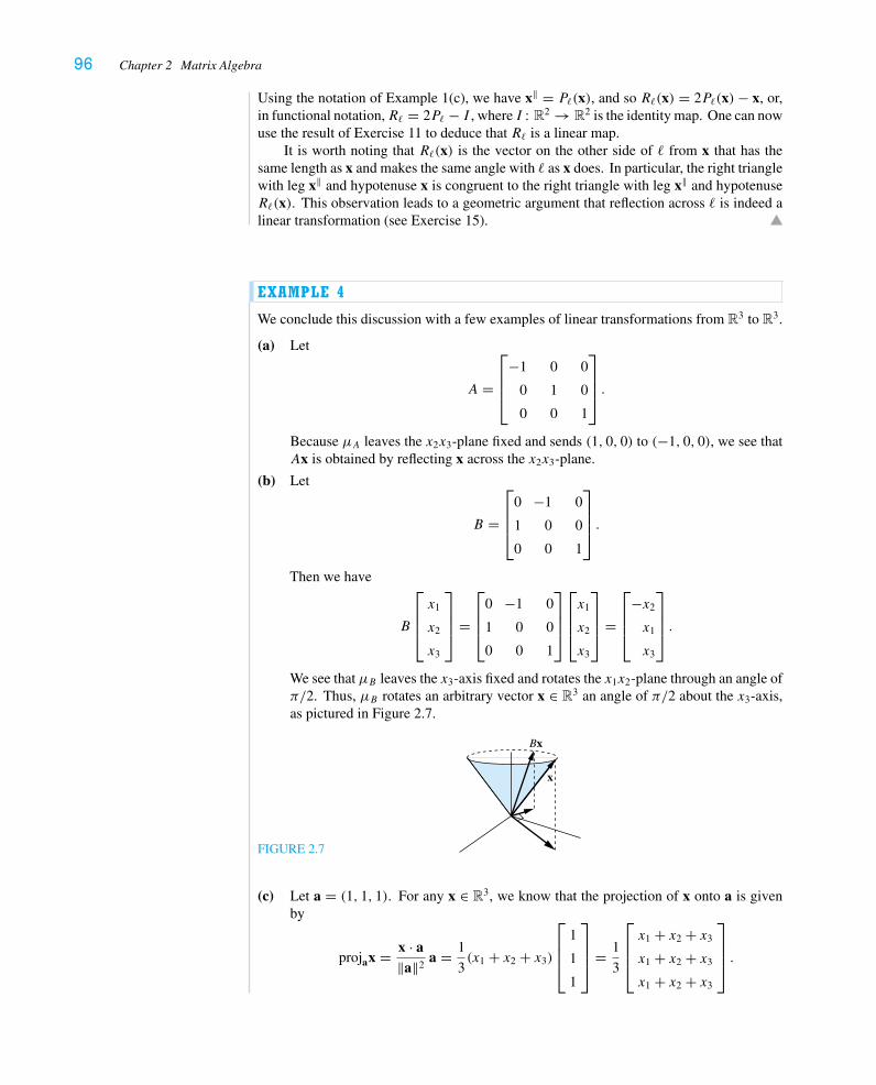
96 Chapter 2 Matrix Algebra
Using the notation of Example 1(c), we have x‖ = P�(x), and so R�(x) = 2P�(x)− x, or,in functional notation,R� = 2P� − I , where I : R2 → R2 is the identity map. One can nowuse the result of Exercise 11 to deduce that R� is a linear map.
It is worth noting that R�(x) is the vector on the other side of � from x that has thesame length as x and makes the same angle with � as x does. In particular, the right trianglewith leg x‖ and hypotenuse x is congruent to the right triangle with leg x‖ and hypotenuseR�(x). This observation leads to a geometric argument that reflection across � is indeed alinear transformation (see Exercise 15).
EXAMPLE 4
We conclude this discussion with a few examples of linear transformations from R3 to R3.
(a) Let
A =
⎡⎢⎢⎣
−1 0 0
0 1 0
0 0 1
⎤⎥⎥⎦ .
Because μA leaves the x2x3-plane fixed and sends (1, 0, 0) to (−1, 0, 0), we see thatAx is obtained by reflecting x across the x2x3-plane.
(b) Let
B =
⎡⎢⎢⎣
0 −1 0
1 0 0
0 0 1
⎤⎥⎥⎦ .
Then we have
B
⎡⎢⎢⎣x1
x2
x3
⎤⎥⎥⎦ =
⎡⎢⎢⎣
0 −1 0
1 0 0
0 0 1
⎤⎥⎥⎦
⎡⎢⎢⎣x1
x2
x3
⎤⎥⎥⎦ =
⎡⎢⎢⎣
−x2
x1
x3
⎤⎥⎥⎦ .
We see that μB leaves the x3-axis fixed and rotates the x1x2-plane through an angle ofπ/2. Thus, μB rotates an arbitrary vector x ∈ R3 an angle of π/2 about the x3-axis,as pictured in Figure 2.7.
FIGURE 2.7
x
Bx
(c) Let a = (1, 1, 1). For any x ∈ R3, we know that the projection of x onto a is givenby
projax = x · a‖a‖2
a = 1
3(x1 + x2 + x3)
⎡⎢⎢⎣
1
1
1
⎤⎥⎥⎦ = 1
3
⎡⎢⎢⎣x1 + x2 + x3
x1 + x2 + x3
x1 + x2 + x3
⎤⎥⎥⎦ .
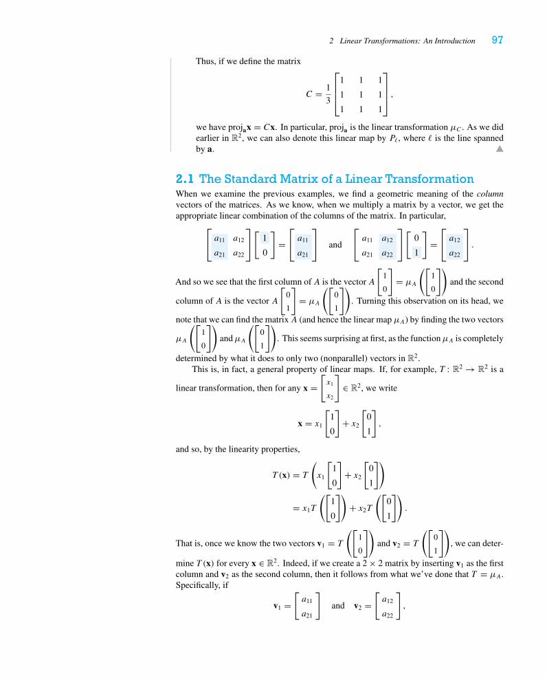
2 Linear Transformations: An Introduction 97
Thus, if we define the matrix
C = 1
3
⎡⎢⎢⎣
1 1 1
1 1 1
1 1 1
⎤⎥⎥⎦ ,
we have projax = Cx. In particular, proja is the linear transformation μC . As we didearlier in R2, we can also denote this linear map by P�, where � is the line spannedby a.
2.1 The Standard Matrix of a Linear TransformationWhen we examine the previous examples, we find a geometric meaning of the columnvectors of the matrices. As we know, when we multiply a matrix by a vector, we get theappropriate linear combination of the columns of the matrix. In particular,
⎡⎣ a11
a21
a12
a22
⎤⎦[
1
0
]=⎡⎣ a11
a21
⎤⎦ and
⎡⎣ a11
a21
a12
a22
⎤⎦[
0
1
]=⎡⎣ a12
a22
⎤⎦ .
And so we see that the first column of A is the vector A
[1
0
]= μA
([1
0
])and the second
column of A is the vector A
[0
1
]= μA
([0
1
]). Turning this observation on its head, we
note that we can find the matrixA (and hence the linear map μA) by finding the two vectors
μA
([1
0
])andμA
([0
1
]). This seems surprising at first, as the functionμA is completely
determined by what it does to only two (nonparallel) vectors in R2.This is, in fact, a general property of linear maps. If, for example, T : R2 → R2 is a
linear transformation, then for any x =[x1
x2
]∈ R2, we write
x = x1
[1
0
]+ x2
[0
1
],
and so, by the linearity properties,
T (x) = T
(x1
[1
0
]+ x2
[0
1
])
= x1T
([1
0
])+ x2T
([0
1
]).
That is, once we know the two vectors v1 = T
([1
0
])and v2 = T
([0
1
]), we can deter-
mine T (x) for every x ∈ R2. Indeed, if we create a 2 × 2 matrix by inserting v1 as the firstcolumn and v2 as the second column, then it follows from what we’ve done that T = μA.Specifically, if
v1 =[a11
a21
]and v2 =
[a12
a22
],
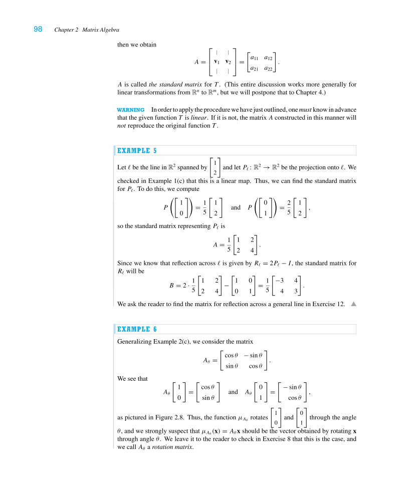
98 Chapter 2 Matrix Algebra
then we obtain
A =⎡⎢⎣ v1 v2
⎤⎥⎦ =
[a11 a12
a21 a22
].
A is called the standard matrix for T . (This entire discussion works more generally forlinear transformations from Rn to Rm, but we will postpone that to Chapter 4.)
WARNING In order to apply the procedure we have just outlined, one must know in advancethat the given function T is linear. If it is not, the matrix A constructed in this manner willnot reproduce the original function T .
EXAMPLE 5
Let � be the line in R2 spanned by
[1
2
]and let P� : R2 → R2 be the projection onto �. We
checked in Example 1(c) that this is a linear map. Thus, we can find the standard matrixfor P�. To do this, we compute
P
([1
0
])= 1
5
[1
2
]and P
([0
1
])= 2
5
[1
2
],
so the standard matrix representing P� is
A = 1
5
[1 2
2 4
].
Since we know that reflection across � is given by R� = 2P� − I , the standard matrix forR� will be
B = 2 · 1
5
[1 2
2 4
]−[
1 0
0 1
]= 1
5
[−3 4
4 3
].
We ask the reader to find the matrix for reflection across a general line in Exercise 12.
EXAMPLE 6
Generalizing Example 2(c), we consider the matrix
Aθ =[
cos θ − sin θ
sin θ cos θ
].
We see that
Aθ
[1
0
]=[
cos θ
sin θ
]and Aθ
[0
1
]=[
− sin θ
cos θ
],
as pictured in Figure 2.8. Thus, the function μAθ rotates
[1
0
]and
[0
1
]through the angle
θ , and we strongly suspect that μAθ (x) = Aθx should be the vector obtained by rotating xthrough angle θ . We leave it to the reader to check in Exercise 8 that this is the case, andwe call Aθ a rotation matrix.
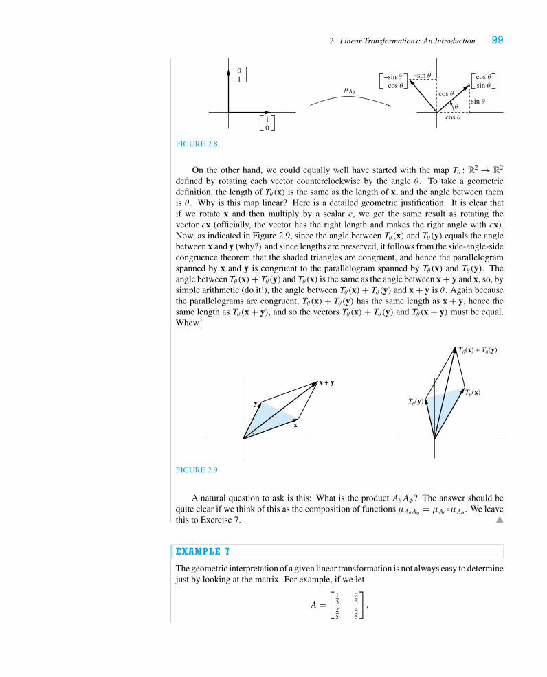
2 Linear Transformations: An Introduction 99
10
01 −sin θ
cos θcos θsin θ
μAθ
−sin θ
sin θcos θ
cos θ
θ
FIGURE 2.8
On the other hand, we could equally well have started with the map Tθ : R2 → R2
defined by rotating each vector counterclockwise by the angle θ . To take a geometricdefinition, the length of Tθ (x) is the same as the length of x, and the angle between themis θ . Why is this map linear? Here is a detailed geometric justification. It is clear thatif we rotate x and then multiply by a scalar c, we get the same result as rotating thevector cx (officially, the vector has the right length and makes the right angle with cx).Now, as indicated in Figure 2.9, since the angle between Tθ (x) and Tθ (y) equals the anglebetween x and y (why?) and since lengths are preserved, it follows from the side-angle-sidecongruence theorem that the shaded triangles are congruent, and hence the parallelogramspanned by x and y is congruent to the parallelogram spanned by Tθ (x) and Tθ (y). Theangle between Tθ (x)+ Tθ (y) and Tθ (x) is the same as the angle between x + y and x, so, bysimple arithmetic (do it!), the angle between Tθ (x)+ Tθ (y) and x + y is θ . Again becausethe parallelograms are congruent, Tθ (x)+ Tθ (y) has the same length as x + y, hence thesame length as Tθ (x + y), and so the vectors Tθ (x)+ Tθ (y) and Tθ (x + y) must be equal.Whew!
y Tθ(y)Tθ(x)
Tθ(x) + Tθ(y)
x
x + y
FIGURE 2.9
A natural question to ask is this: What is the product AθAφ? The answer should bequite clear if we think of this as the composition of functions μAθAφ = μAθ ◦μAφ . We leavethis to Exercise 7.
EXAMPLE 7
The geometric interpretation of a given linear transformation is not always easy to determinejust by looking at the matrix. For example, if we let
A =[
15
25
25
45
],
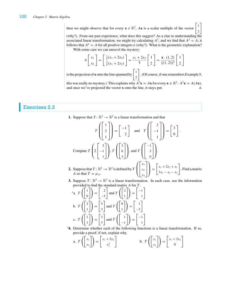
100 Chapter 2 Matrix Algebra
then we might observe that for every x ∈ R2, Ax is a scalar multiple of the vector
[1
2
]
(why?). From our past experience, what does this suggest? As a clue to understanding theassociated linear transformation, we might try calculating A2, and we find that A2 = A; itfollows that An = A for all positive integers n (why?). What is the geometric explanation?
With some care we can unravel the mystery:
A
[x1
x2
]=[
15 (x1 + 2x2)
25 (x1 + 2x2)
]= x1 + 2x2
5
[1
2
]= x · (1, 2)
‖(1, 2)‖2
[1
2
]
is the projection of x onto the line spanned by
[1
2
]. (Of course, if one remembers Example 5,
this was really no mystery.) This explains whyA2x = Ax for every x ∈ R2: A2x = A(Ax),and once we’ve projected the vector x onto the line, it stays put.
Exercises 2.2
1. Suppose that T : R3 → R2 is a linear transformation and that
T
⎛⎜⎜⎝
⎡⎢⎢⎣
1
2
1
⎤⎥⎥⎦
⎞⎟⎟⎠ =
[−1
2
]and T
⎛⎜⎜⎝
⎡⎢⎢⎣
2
−1
1
⎤⎥⎥⎦
⎞⎟⎟⎠ =
[3
0
].
Compute T
⎛⎜⎝2
⎡⎢⎣
2
−1
1
⎤⎥⎦
⎞⎟⎠, T
⎛⎜⎝
⎡⎢⎣
3
6
3
⎤⎥⎦
⎞⎟⎠, and T
⎛⎜⎝
⎡⎢⎣
−1
3
0
⎤⎥⎦
⎞⎟⎠.
2. Suppose thatT : R3 → R2 is defined byT
⎛⎜⎝
⎡⎢⎣x1
x2
x3
⎤⎥⎦
⎞⎟⎠ =
[x1 + 2x2 + x3
3x1 − x2 − x3
]. Find a matrix
A so that T = μA.
3. Suppose T : R2 → R2 is a linear transformation. In each case, use the informationprovided to find the standard matrix A for T .
a.∗ T
([1
0
])=[
2
−3
]and T
([2
1
])=[
−1
1
]
b. T
([2
1
])=[
5
3
]and T
([0
1
])=[
1
−3
]
c. T
([1
1
])=[
3
3
]and T
([1
−1
])=[
−1
1
]
4.∗ Determine whether each of the following functions is a linear transformation. If so,provide a proof; if not, explain why.
a. T
([x1
x2
])=[x1 + 2x2
x22
]b. T
([x1
x2
])=[x1 + 2x2
0
]
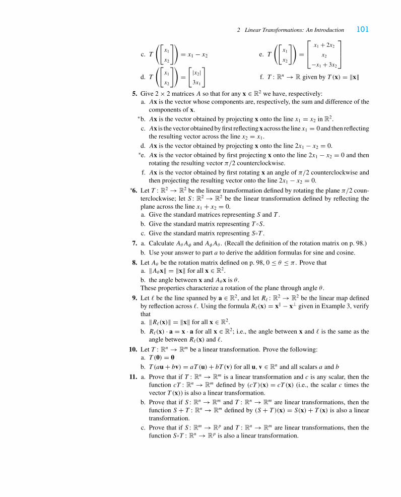
2 Linear Transformations: An Introduction 101
c. T
([x1
x2
])= x1 − x2
d. T
([x1
x2
])=[
|x2|3x1
]e. T
([x1
x2
])=⎡⎢⎣x1 + 2x2
x2
−x1 + 3x2
⎤⎥⎦
f. T : Rn → R given by T (x) = ‖x‖
5. Give 2 × 2 matrices A so that for any x ∈ R2 we have, respectively:a. Ax is the vector whose components are, respectively, the sum and difference of the
components of x.
b.∗ Ax is the vector obtained by projecting x onto the line x1 = x2 in R2.
c. Ax is the vector obtained by first reflecting x across the linex1 = 0 and then reflectingthe resulting vector across the line x2 = x1.
d. Ax is the vector obtained by projecting x onto the line 2x1 − x2 = 0.
e.∗ Ax is the vector obtained by first projecting x onto the line 2x1 − x2 = 0 and thenrotating the resulting vector π/2 counterclockwise.
f. Ax is the vector obtained by first rotating x an angle of π/2 counterclockwise andthen projecting the resulting vector onto the line 2x1 − x2 = 0.
6.∗ Let T : R2 → R2 be the linear transformation defined by rotating the plane π/2 coun-terclockwise; let S : R2 → R2 be the linear transformation defined by reflecting theplane across the line x1 + x2 = 0.a. Give the standard matrices representing S and T .
b. Give the standard matrix representing T ◦S.
c. Give the standard matrix representing S◦T .
7. a. Calculate AθAφ and AφAθ . (Recall the definition of the rotation matrix on p. 98.)
b. Use your answer to part a to derive the addition formulas for sine and cosine.
8. Let Aθ be the rotation matrix defined on p. 98, 0 ≤ θ ≤ π . Prove thata. ‖Aθx‖ = ‖x‖ for all x ∈ R2.
b. the angle between x and Aθx is θ .These properties characterize a rotation of the plane through angle θ .
9. Let � be the line spanned by a ∈ R2, and let R� : R2 → R2 be the linear map definedby reflection across �. Using the formula R�(x) = x‖ − x⊥ given in Example 3, verifythata. ‖R�(x)‖ = ‖x‖ for all x ∈ R2.
b. R�(x) · a = x · a for all x ∈ R2; i.e., the angle between x and � is the same as theangle between R�(x) and �.
10. Let T : Rn → Rm be a linear transformation. Prove the following:a. T (0) = 0b. T (au + bv) = aT (u)+ bT (v) for all u, v ∈ Rn and all scalars a and b
11. a. Prove that if T : Rn → Rm is a linear transformation and c is any scalar, then thefunction cT : Rn → Rm defined by (cT )(x) = cT (x) (i.e., the scalar c times thevector T (x)) is also a linear transformation.
b. Prove that if S : Rn → Rm and T : Rn → Rm are linear transformations, then thefunction S + T : Rn → Rm defined by (S + T )(x) = S(x)+ T (x) is also a lineartransformation.
c. Prove that if S : Rm → Rp and T : Rn → Rm are linear transformations, then thefunction S◦T : Rn → Rp is also a linear transformation.
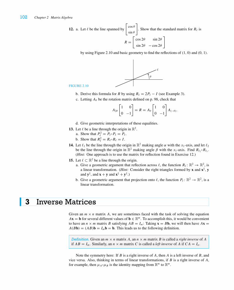
102 Chapter 2 Matrix Algebra
12. a. Let � be the line spanned by
[cos θ
sin θ
]. Show that the standard matrix for R� is
R =[
cos 2θ sin 2θ
sin 2θ − cos 2θ
]
by using Figure 2.10 and basic geometry to find the reflections of (1, 0) and (0, 1).
FIGURE 2.10
θ
�
b. Derive this formula for R by using R� = 2P� − I (see Example 3).
c. Letting Aθ be the rotation matrix defined on p. 98, check that
A2θ
[1 0
0 −1
]= R = Aθ
[1 0
0 −1
]A(−θ).
d. Give geometric interpretations of these equalities.
13. Let � be a line through the origin in R2.a. Show that P 2
� = P�◦P� = P�.
b. Show that R2� = R�◦R� = I .
14. Let �1 be the line through the origin in R2 making angle α with the x1-axis, and let �2
be the line through the origin in R2 making angle β with the x1-axis. Find R�2◦R�1 .
(Hint: One approach is to use the matrix for reflection found in Exercise 12.)
15. Let � ⊂ R2 be a line through the origin.a. Give a geometric argument that reflection across �, the function R� : R2 → R2, is
a linear transformation. (Hint: Consider the right triangles formed by x and x‖, yand y‖, and x + y and x‖ + y‖.)
b. Give a geometric argument that projection onto �, the function P� : R2 → R2, is alinear transformation.
3 Inverse MatricesGiven an m× n matrix A, we are sometimes faced with the task of solving the equationAx = b for several different values of b ∈ Rm. To accomplish this, it would be convenientto have an n×m matrix B satisfying AB = Im: Taking x = Bb, we will then have Ax =A(Bb) = (AB)b = Imb = b. This leads us to the following definition.
Definition. Given an m× n matrix A, an n×m matrix B is called a right inverse of Aif AB = Im. Similarly, an n×m matrix C is called a left inverse of A if CA = In.
Note the symmetry here: If B is a right inverse of A, then A is a left inverse of B, andvice versa. Also, thinking in terms of linear transformations, if B is a right inverse of A,for example, then μA◦μB is the identity mapping from Rm to Rm.
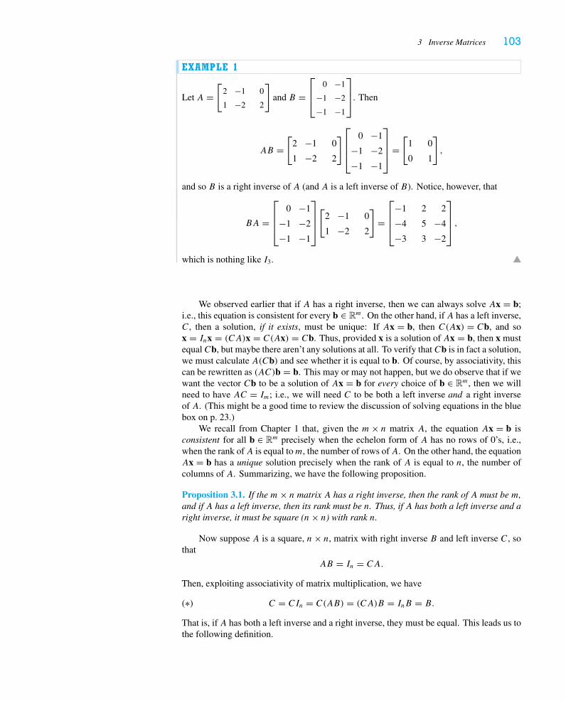
3 Inverse Matrices 103
EXAMPLE 1
Let A =[
2 −1 0
1 −2 2
]and B =
⎡⎢⎣
0 −1
−1 −2
−1 −1
⎤⎥⎦. Then
AB =[
2 −1 0
1 −2 2
]⎡⎢⎢⎣0 −1
−1 −2
−1 −1
⎤⎥⎥⎦ =
[1 0
0 1
],
and so B is a right inverse of A (and A is a left inverse of B). Notice, however, that
BA =
⎡⎢⎢⎣
0 −1
−1 −2
−1 −1
⎤⎥⎥⎦[
2 −1 0
1 −2 2
]=
⎡⎢⎢⎣
−1 2 2
−4 5 −4
−3 3 −2
⎤⎥⎥⎦ ,
which is nothing like I3.
We observed earlier that if A has a right inverse, then we can always solve Ax = b;i.e., this equation is consistent for every b ∈ Rm. On the other hand, if A has a left inverse,C, then a solution, if it exists, must be unique: If Ax = b, then C(Ax) = Cb, and sox = Inx = (CA)x = C(Ax) = Cb. Thus, provided x is a solution of Ax = b, then x mustequal Cb, but maybe there aren’t any solutions at all. To verify that Cb is in fact a solution,we must calculate A(Cb) and see whether it is equal to b. Of course, by associativity, thiscan be rewritten as (AC)b = b. This may or may not happen, but we do observe that if wewant the vector Cb to be a solution of Ax = b for every choice of b ∈ Rm, then we willneed to have AC = Im; i.e., we will need C to be both a left inverse and a right inverseof A. (This might be a good time to review the discussion of solving equations in the bluebox on p. 23.)
We recall from Chapter 1 that, given the m× n matrix A, the equation Ax = b isconsistent for all b ∈ Rm precisely when the echelon form of A has no rows of 0’s, i.e.,when the rank ofA is equal tom, the number of rows ofA. On the other hand, the equationAx = b has a unique solution precisely when the rank of A is equal to n, the number ofcolumns of A. Summarizing, we have the following proposition.
Proposition 3.1. If the m× n matrix A has a right inverse, then the rank of A must be m,and if A has a left inverse, then its rank must be n. Thus, if A has both a left inverse and aright inverse, it must be square (n× n) with rank n.
Now suppose A is a square, n× n, matrix with right inverse B and left inverse C, sothat
AB = In = CA.
Then, exploiting associativity of matrix multiplication, we have
(∗) C = CIn = C(AB) = (CA)B = InB = B.
That is, if A has both a left inverse and a right inverse, they must be equal. This leads us tothe following definition.
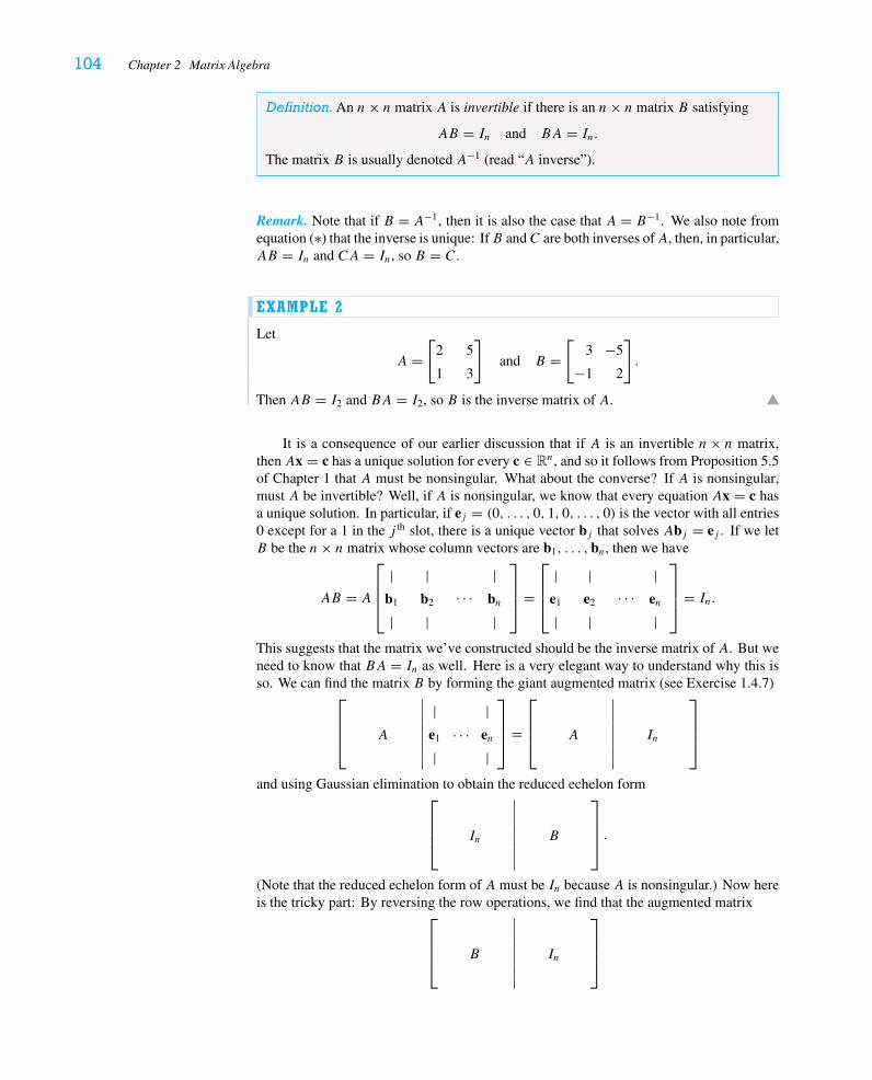
104 Chapter 2 Matrix Algebra
Definition.An n× n matrix A is invertible if there is an n× n matrix B satisfying
AB = In and BA = In.
The matrix B is usually denoted A−1 (read “A inverse”).
Remark. Note that if B = A−1, then it is also the case that A = B−1. We also note fromequation (∗) that the inverse is unique: IfB andC are both inverses ofA, then, in particular,AB = In and CA = In, so B = C.
EXAMPLE 2
Let
A =[
2 5
1 3
]and B =
[3 −5
−1 2
].
Then AB = I2 and BA = I2, so B is the inverse matrix of A.
It is a consequence of our earlier discussion that if A is an invertible n× n matrix,then Ax = c has a unique solution for every c ∈ Rn, and so it follows from Proposition 5.5of Chapter 1 that A must be nonsingular. What about the converse? If A is nonsingular,must A be invertible? Well, if A is nonsingular, we know that every equation Ax = c hasa unique solution. In particular, if ej = (0, . . . , 0, 1, 0, . . . , 0) is the vector with all entries0 except for a 1 in the j th slot, there is a unique vector bj that solves Abj = ej . If we letB be the n× n matrix whose column vectors are b1, . . . ,bn, then we have
AB = A
⎡⎢⎢⎣
|b1
|
|b2
|· · ·
|bn
|
⎤⎥⎥⎦ =
⎡⎢⎢⎣
|e1
|
|e2
|· · ·
|en
|
⎤⎥⎥⎦ = In.
This suggests that the matrix we’ve constructed should be the inverse matrix of A. But weneed to know that BA = In as well. Here is a very elegant way to understand why this isso. We can find the matrix B by forming the giant augmented matrix (see Exercise 1.4.7)⎡
⎢⎢⎣| |
A e1 · · · en
| |
⎤⎥⎥⎦ =
⎡⎢⎢⎣ A In
⎤⎥⎥⎦
and using Gaussian elimination to obtain the reduced echelon form⎡⎢⎢⎣ In B
⎤⎥⎥⎦ .
(Note that the reduced echelon form of A must be In because A is nonsingular.) Now hereis the tricky part: By reversing the row operations, we find that the augmented matrix⎡
⎢⎢⎣ B In
⎤⎥⎥⎦
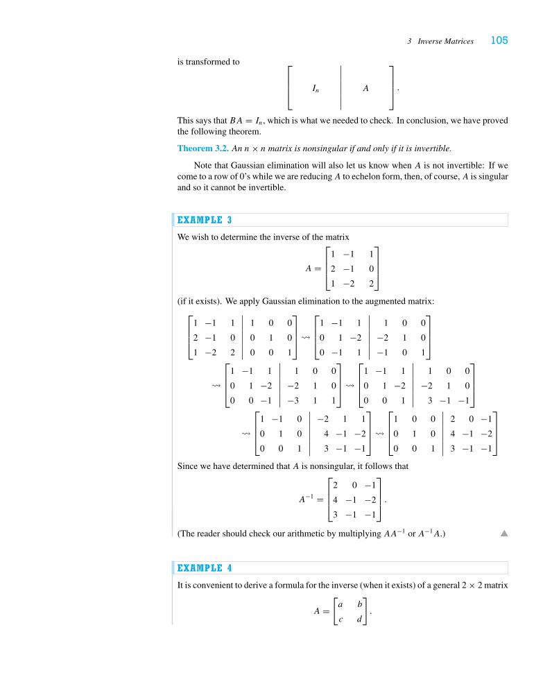
3 Inverse Matrices 105
is transformed to ⎡⎢⎢⎣ In A
⎤⎥⎥⎦ .
This says that BA = In, which is what we needed to check. In conclusion, we have provedthe following theorem.
Theorem 3.2. An n× n matrix is nonsingular if and only if it is invertible.
Note that Gaussian elimination will also let us know when A is not invertible: If wecome to a row of 0’s while we are reducingA to echelon form, then, of course,A is singularand so it cannot be invertible.
EXAMPLE 3
We wish to determine the inverse of the matrix
A =
⎡⎢⎢⎣
1 −1 1
2 −1 0
1 −2 2
⎤⎥⎥⎦
(if it exists). We apply Gaussian elimination to the augmented matrix:⎡⎢⎢⎣
1 −1 1 1 0 0
2 −1 0 0 1 0
1 −2 2 0 0 1
⎤⎥⎥⎦�
⎡⎢⎢⎣
1 −1 1 1 0 0
0 1 −2 −2 1 0
0 −1 1 −1 0 1
⎤⎥⎥⎦
�
⎡⎢⎢⎣
1 −1 1 1 0 0
0 1 −2 −2 1 0
0 0 −1 −3 1 1
⎤⎥⎥⎦�
⎡⎢⎢⎣
1 −1 1 1 0 0
0 1 −2 −2 1 0
0 0 1 3 −1 −1
⎤⎥⎥⎦
�
⎡⎢⎢⎣
1 −1 0 −2 1 1
0 1 0 4 −1 −2
0 0 1 3 −1 −1
⎤⎥⎥⎦�
⎡⎢⎢⎣
1 0 0 2 0 −1
0 1 0 4 −1 −2
0 0 1 3 −1 −1
⎤⎥⎥⎦
Since we have determined that A is nonsingular, it follows that
A−1 =
⎡⎢⎢⎣
2 0 −1
4 −1 −2
3 −1 −1
⎤⎥⎥⎦ .
(The reader should check our arithmetic by multiplying AA−1 or A−1A.)
EXAMPLE 4
It is convenient to derive a formula for the inverse (when it exists) of a general 2 × 2 matrix
A =[a b
c d
].
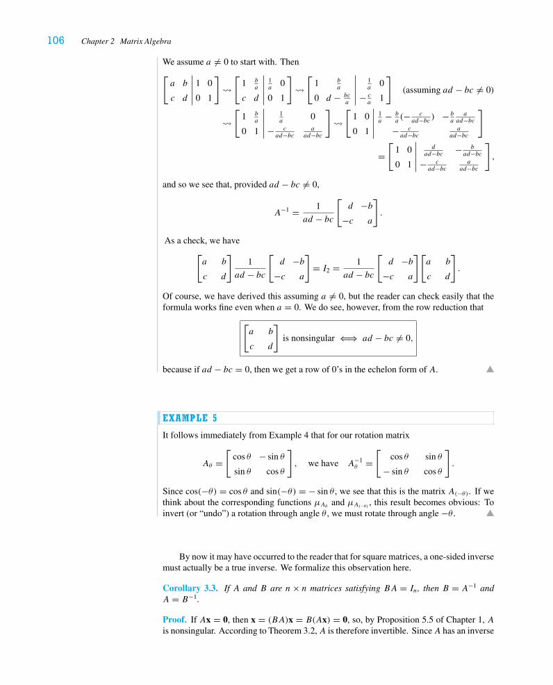
106 Chapter 2 Matrix Algebra
We assume a �= 0 to start with. Then[a b 1 0
c d 0 1
]�[
1 ba
1a
0
c d 0 1
]�[
1 ba
1a
0
0 d − bca
− ca
1
](assuming ad − bc �= 0)
�[
1 ba
1a
0
0 1 − cad−bc
aad−bc
]�[
1 0 1a
− ba(− c
ad−bc ) − ba
aad−bc
0 1 − cad−bc
aad−bc
]
=[
1 0 dad−bc − b
ad−bc0 1 − c
ad−bca
ad−bc
],
and so we see that, provided ad − bc �= 0,
A−1 = 1
ad − bc
[d −b
−c a
].
As a check, we have[a b
c d
]1
ad − bc
[d −b
−c a
]= I2 = 1
ad − bc
[d −b
−c a
][a b
c d
].
Of course, we have derived this assuming a �= 0, but the reader can check easily that theformula works fine even when a = 0. We do see, however, from the row reduction that
[a b
c d
]is nonsingular ⇐⇒ ad − bc �= 0,
because if ad − bc = 0, then we get a row of 0’s in the echelon form of A.
EXAMPLE 5
It follows immediately from Example 4 that for our rotation matrix
Aθ =[
cos θ − sin θ
sin θ cos θ
], we have A−1
θ =[
cos θ sin θ
− sin θ cos θ
].
Since cos(−θ) = cos θ and sin(−θ) = − sin θ , we see that this is the matrix A(−θ). If wethink about the corresponding functions μAθ and μA(−θ) , this result becomes obvious: Toinvert (or “undo”) a rotation through angle θ , we must rotate through angle −θ .
By now it may have occurred to the reader that for square matrices, a one-sided inversemust actually be a true inverse. We formalize this observation here.
Corollary 3.3. If A and B are n× n matrices satisfying BA = In, then B = A−1 andA = B−1.
Proof. If Ax = 0, then x = (BA)x = B(Ax) = 0, so, by Proposition 5.5 of Chapter 1, Ais nonsingular. According to Theorem 3.2,A is therefore invertible. SinceA has an inverse
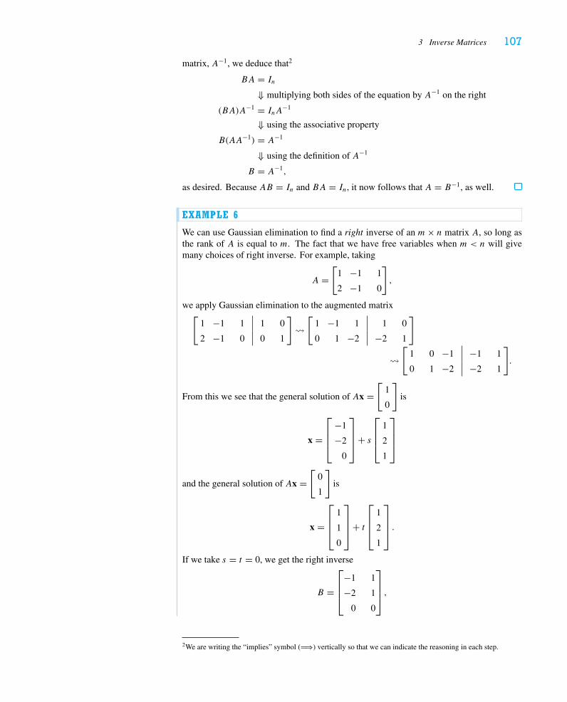
3 Inverse Matrices 107
matrix, A−1, we deduce that2
BA = In
⇓ multiplying both sides of the equation by A−1 on the right
(BA)A−1 = InA−1
⇓ using the associative property
B(AA−1) = A−1
⇓ using the definition of A−1
B = A−1,
as desired. Because AB = In and BA = In, it now follows that A = B−1, as well.
EXAMPLE 6
We can use Gaussian elimination to find a right inverse of an m× n matrix A, so long asthe rank of A is equal to m. The fact that we have free variables when m < n will givemany choices of right inverse. For example, taking
A =[
1 −1 1
2 −1 0
],
we apply Gaussian elimination to the augmented matrix[
1 −1 1 1 0
2 −1 0 0 1
]�[
1 −1 1 1 0
0 1 −2 −2 1
]
�[
1 0 −1 −1 1
0 1 −2 −2 1
].
From this we see that the general solution of Ax =[
1
0
]is
x =
⎡⎢⎢⎣
−1
−2
0
⎤⎥⎥⎦+ s
⎡⎢⎢⎣
1
2
1
⎤⎥⎥⎦
and the general solution of Ax =[
0
1
]is
x =
⎡⎢⎢⎣
1
1
0
⎤⎥⎥⎦+ t
⎡⎢⎢⎣
1
2
1
⎤⎥⎥⎦ .
If we take s = t = 0, we get the right inverse
B =
⎡⎢⎢⎣
−1 1
−2 1
0 0
⎤⎥⎥⎦ ,
2We are writing the “implies” symbol (�⇒) vertically so that we can indicate the reasoning in each step.
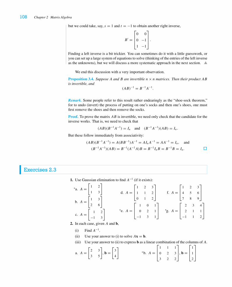
108 Chapter 2 Matrix Algebra
but we could take, say, s = 1 and t = −1 to obtain another right inverse,
B ′ =
⎡⎢⎢⎣
0 0
0 −1
1 −1
⎤⎥⎥⎦ .
Finding a left inverse is a bit trickier. You can sometimes do it with a little guesswork, oryou can set up a large system of equations to solve (thinking of the entries of the left inverseas the unknowns), but we will discuss a more systematic approach in the next section.
We end this discussion with a very important observation.
Proposition 3.4. Suppose A and B are invertible n× n matrices. Then their product ABis invertible, and
(AB)−1 = B−1A−1.
Remark. Some people refer to this result rather endearingly as the “shoe-sock theorem,”for to undo (invert) the process of putting on one’s socks and then one’s shoes, one mustfirst remove the shoes and then remove the socks.
Proof. To prove the matrix AB is invertible, we need only check that the candidate for theinverse works. That is, we need to check that
(AB)(B−1A−1) = In and (B−1A−1)(AB) = In.
But these follow immediately from associativity:
(AB)(B−1A−1) = A(BB−1)A−1 = AInA−1 = AA−1 = In, and
(B−1A−1)(AB) = B−1(A−1A)B = B−1InB = B−1B = In.
Exercises 2.3
1. Use Gaussian elimination to find A−1 (if it exists):
a.∗ A =[
1 2
1 3
]
b. A =[
1 3
2 6
]
c. A =[
1 2
−1 3
]
d. A =⎡⎢⎣
1 2 3
1 1 2
0 1 2
⎤⎥⎦
e.∗ A =⎡⎢⎣
1 0 1
0 2 1
−1 3 1
⎤⎥⎦
f. A =⎡⎢⎣
1 2 3
4 5 6
7 8 9
⎤⎥⎦
g.∗ A =⎡⎢⎣
2 3 4
2 1 1
−1 1 2
⎤⎥⎦
2. In each case, given A and b,
(i) Find A−1.
(ii) Use your answer to (i) to solve Ax = b.
(iii) Use your answer to (ii) to express b as a linear combination of the columns ofA.
a. A =[
2 3
3 5
], b =
[3
4
]b.∗ A =
⎡⎢⎣
1 1 1
0 2 3
3 2 2
⎤⎥⎦, b =
⎡⎢⎣
1
1
2
⎤⎥⎦
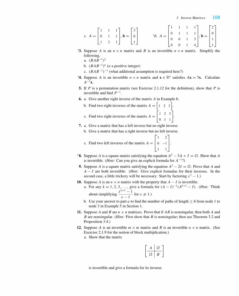
3 Inverse Matrices 109
c. A =⎡⎢⎣
1 1 1
0 1 1
1 2 1
⎤⎥⎦, b =
⎡⎢⎣
3
0
1
⎤⎥⎦ d.∗ A =
⎡⎢⎢⎢⎣
1 1 1 1
0 1 1 1
0 0 1 3
0 0 1 4
⎤⎥⎥⎥⎦, b =
⎡⎢⎢⎢⎣
2
0
1
1
⎤⎥⎥⎥⎦
3.∗ Suppose A is an n× n matrix and B is an invertible n× n matrix. Simplify thefollowing.a. (BAB−1)2
b. (BAB−1)n (n a positive integer)
c. (BAB−1)−1 (what additional assumption is required here?)
4.∗ Suppose A is an invertible n× n matrix and x ∈ Rn satisfies Ax = 7x. CalculateA−1x.
5. If P is a permutation matrix (see Exercise 2.1.12 for the definition), show that P isinvertible and find P−1.
6. a. Give another right inverse of the matrix A in Example 6.
b. Find two right inverses of the matrix A =[
1 2 3].
c. Find two right inverses of the matrix A =[
1 2 3
0 1 1
].
7. a. Give a matrix that has a left inverse but no right inverse.
b. Give a matrix that has a right inverse but no left inverse.
c. Find two left inverses of the matrix A =⎡⎢⎣
1 2
0 −1
1 1
⎤⎥⎦.
8.∗ Suppose A is a square matrix satisfying the equation A3 − 3A+ I = O. Show that Ais invertible. (Hint: Can you give an explicit formula for A−1?)
9. Suppose A is a square matrix satisfying the equation A3 − 2I = O. Prove that A andA− I are both invertible. (Hint: Give explicit formulas for their inverses. In thesecond case, a little trickery will be necessary: Start by factoring x3 − 1.)
10. Suppose A is an n× n matrix with the property that A− I is invertible.a. For any k = 1, 2, 3, . . . , give a formula for (A− I )−1(Ak+1 − I ). (Hint: Think
about simplifyingxk+1 − 1
x − 1for x �= 1.)
b. Use your answer to part a to find the number of paths of length ≤ 6 from node 1 tonode 3 in Example 5 in Section 1.
11. SupposeA and B are n× nmatrices. Prove that ifAB is nonsingular, then bothA andB are nonsingular. (Hint: First show that B is nonsingular; then use Theorem 3.2 andProposition 3.4.)
12. Suppose A is an invertible m×m matrix and B is an invertible n× n matrix. (SeeExercise 2.1.9 for the notion of block multiplication.)a. Show that the matrix
[A O
O B
]
is invertible and give a formula for its inverse.
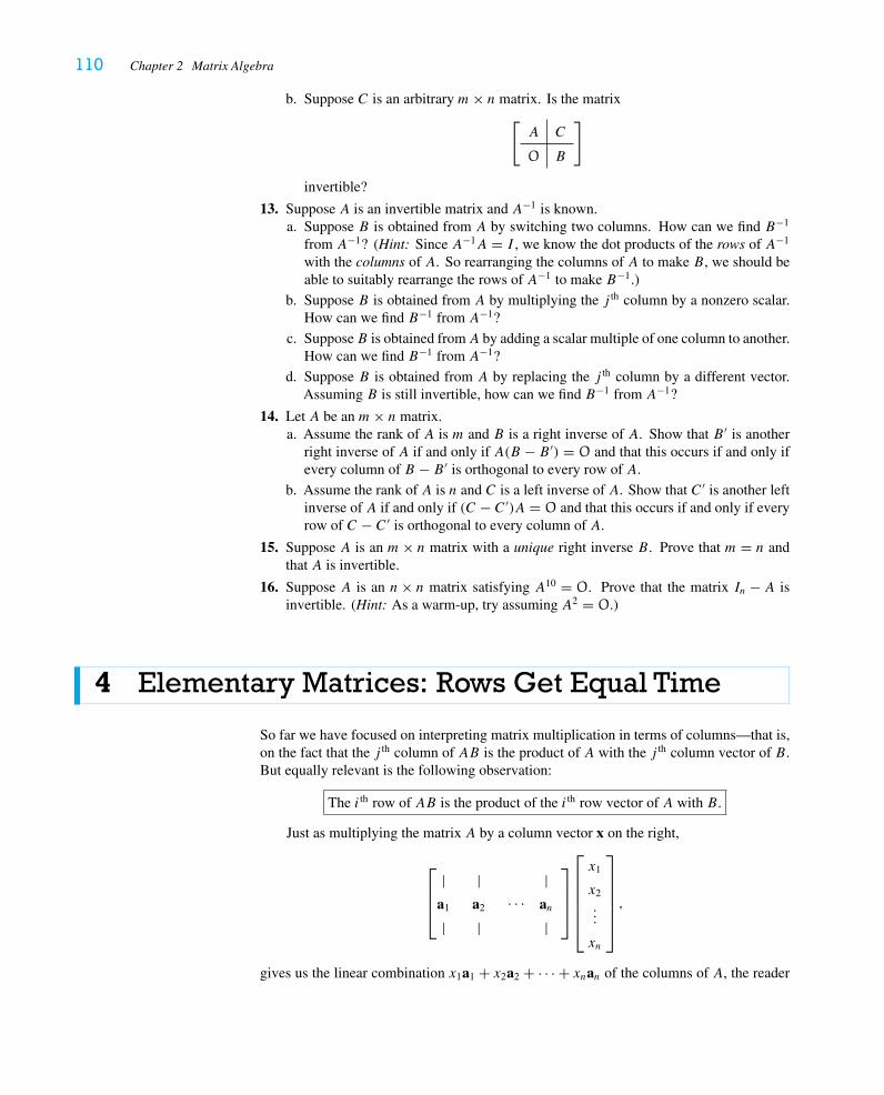
110 Chapter 2 Matrix Algebra
b. Suppose C is an arbitrary m× n matrix. Is the matrix[A C
O B
]
invertible?
13. Suppose A is an invertible matrix and A−1 is known.a. Suppose B is obtained from A by switching two columns. How can we find B−1
from A−1? (Hint: Since A−1A = I , we know the dot products of the rows of A−1
with the columns of A. So rearranging the columns of A to make B, we should beable to suitably rearrange the rows of A−1 to make B−1.)
b. Suppose B is obtained from A by multiplying the j th column by a nonzero scalar.How can we find B−1 from A−1?
c. SupposeB is obtained fromA by adding a scalar multiple of one column to another.How can we find B−1 from A−1?
d. Suppose B is obtained from A by replacing the j th column by a different vector.Assuming B is still invertible, how can we find B−1 from A−1?
14. Let A be an m× n matrix.a. Assume the rank of A is m and B is a right inverse of A. Show that B ′ is another
right inverse of A if and only if A(B − B ′) = O and that this occurs if and only ifevery column of B − B ′ is orthogonal to every row of A.
b. Assume the rank of A is n and C is a left inverse of A. Show that C ′ is another leftinverse of A if and only if (C − C ′)A = O and that this occurs if and only if everyrow of C − C ′ is orthogonal to every column of A.
15. Suppose A is an m× n matrix with a unique right inverse B. Prove that m = n andthat A is invertible.
16. Suppose A is an n× n matrix satisfying A10 = O. Prove that the matrix In − A isinvertible. (Hint: As a warm-up, try assuming A2 = O.)
4 Elementary Matrices: Rows Get Equal Time
So far we have focused on interpreting matrix multiplication in terms of columns—that is,on the fact that the j th column of AB is the product of A with the j th column vector of B.But equally relevant is the following observation:
The i th row of AB is the product of the i th row vector of A with B.
Just as multiplying the matrix A by a column vector x on the right,
⎡⎢⎢⎣
|a1
|
|a2
|· · ·
|an
|
⎤⎥⎥⎦
⎡⎢⎢⎢⎢⎢⎣
x1
x2
...
xn
⎤⎥⎥⎥⎥⎥⎦,
gives us the linear combination x1a1 + x2a2 + · · · + xnan of the columns of A, the reader
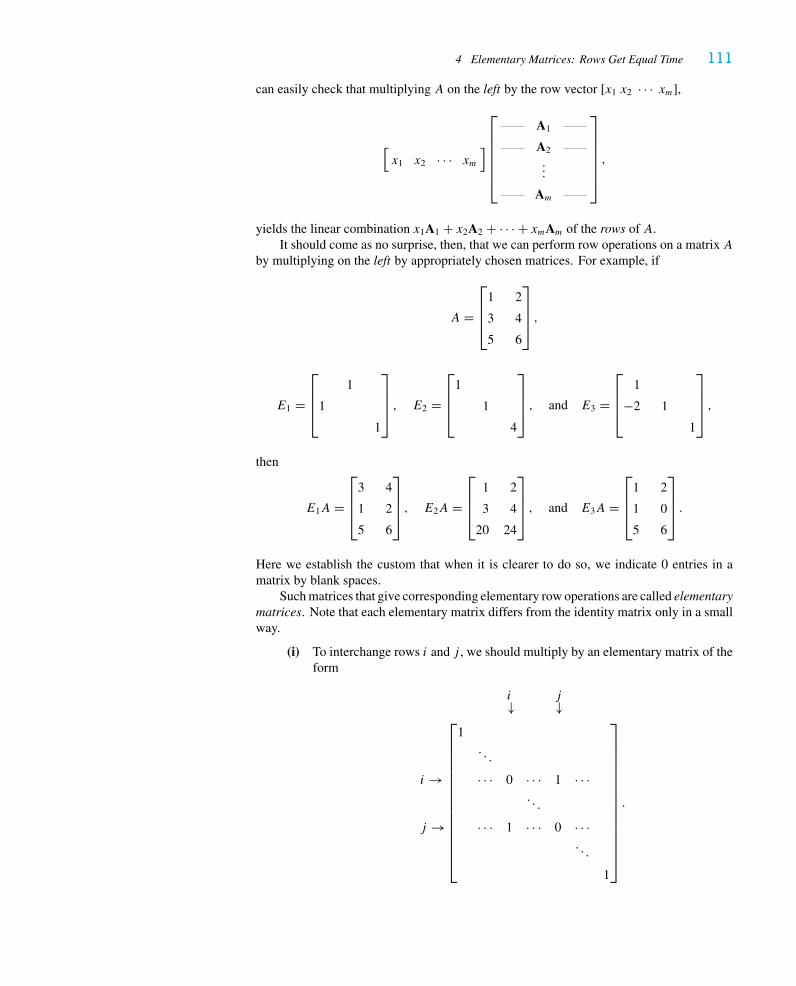
4 Elementary Matrices: Rows Get Equal Time 111
can easily check that multiplying A on the left by the row vector [x1 x2 · · · xm],
[x1 x2 · · · xm
]
⎡⎢⎢⎢⎢⎢⎣
A1
A2
...
Am
⎤⎥⎥⎥⎥⎥⎦,
yields the linear combination x1A1 + x2A2 + · · · + xmAm of the rows of A.It should come as no surprise, then, that we can perform row operations on a matrix A
by multiplying on the left by appropriately chosen matrices. For example, if
A =
⎡⎢⎢⎣
1 2
3 4
5 6
⎤⎥⎥⎦ ,
E1 =
⎡⎢⎢⎣
1
1
1
⎤⎥⎥⎦ , E2 =
⎡⎢⎢⎣
1
1
4
⎤⎥⎥⎦ , and E3 =
⎡⎢⎢⎣
1
−2 1
1
⎤⎥⎥⎦ ,
then
E1A =
⎡⎢⎢⎣
3 4
1 2
5 6
⎤⎥⎥⎦ , E2A =
⎡⎢⎢⎣
1 2
3 4
20 24
⎤⎥⎥⎦ , and E3A =
⎡⎢⎢⎣
1 2
1 0
5 6
⎤⎥⎥⎦ .
Here we establish the custom that when it is clearer to do so, we indicate 0 entries in amatrix by blank spaces.
Such matrices that give corresponding elementary row operations are called elementarymatrices. Note that each elementary matrix differs from the identity matrix only in a smallway.
(i) To interchange rows i and j , we should multiply by an elementary matrix of theform
i↓ j↓
i →
j →
⎡⎢⎢⎢⎢⎢⎢⎢⎢⎢⎢⎢⎢⎢⎢⎣
1. . .
· · · 0 · · · 1 · · ·. . .
· · · 1 · · · 0 · · ·. . .
1
⎤⎥⎥⎥⎥⎥⎥⎥⎥⎥⎥⎥⎥⎥⎥⎦
.
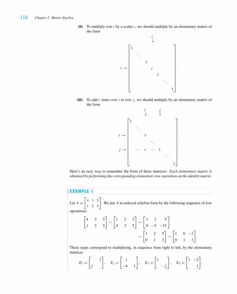
112 Chapter 2 Matrix Algebra
(ii) To multiply row i by a scalar c, we should multiply by an elementary matrix ofthe form
i↓
i →
⎡⎢⎢⎢⎢⎢⎢⎢⎢⎢⎢⎢⎢⎢⎢⎣
1. . .
1
c
1. . .
1
⎤⎥⎥⎥⎥⎥⎥⎥⎥⎥⎥⎥⎥⎥⎥⎦
.
(iii) To add c times row i to row j , we should multiply by an elementary matrix ofthe form
i↓ j↓
i →
j →
⎡⎢⎢⎢⎢⎢⎢⎢⎢⎢⎢⎢⎢⎢⎢⎣
1. . .
1. . .
· · · c · · · 1. . .
1
⎤⎥⎥⎥⎥⎥⎥⎥⎥⎥⎥⎥⎥⎥⎥⎦
.
Here’s an easy way to remember the form of these matrices: Each elementary matrix isobtained by performing the corresponding elementary row operation on the identity matrix.
EXAMPLE 1
Let A =[
4 3 5
1 2 5
]. We put A in reduced echelon form by the following sequence of row
operations:[
4 3 5
1 2 5
]�[
1 2 5
4 3 5
]�[
1 2 5
0 −5 −15
]
�[
1 2 5
0 1 3
]�[
1 0 −1
0 1 3
].
These steps correspond to multiplying, in sequence from right to left, by the elementarymatrices
E1 =[
1
1
], E2 =
[1
−4 1
], E3 =
[1
− 15
], E4 =
[1 −2
1
].
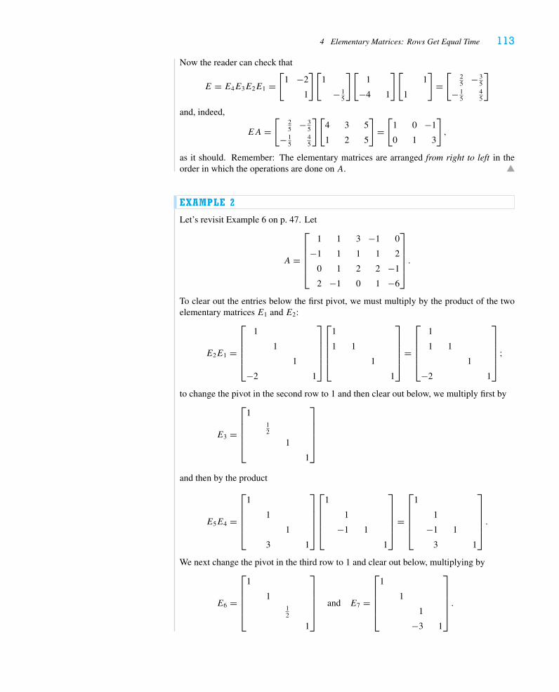
4 Elementary Matrices: Rows Get Equal Time 113
Now the reader can check that
E = E4E3E2E1 =[
1 −2
1
][1
− 15
][1
−4 1
][1
1
]=[
25 − 3
5
− 15
45
]
and, indeed,
EA =[
25 − 3
5
− 15
45
][4 3 5
1 2 5
]=[
1 0 −1
0 1 3
],
as it should. Remember: The elementary matrices are arranged from right to left in theorder in which the operations are done on A.
EXAMPLE 2
Let’s revisit Example 6 on p. 47. Let
A =
⎡⎢⎢⎢⎢⎣
1 1 3 −1 0
−1 1 1 1 2
0 1 2 2 −1
2 −1 0 1 −6
⎤⎥⎥⎥⎥⎦.
To clear out the entries below the first pivot, we must multiply by the product of the twoelementary matrices E1 and E2:
E2E1 =
⎡⎢⎢⎢⎢⎣
1
1
1
−2 1
⎤⎥⎥⎥⎥⎦
⎡⎢⎢⎢⎢⎣
1
1 1
1
1
⎤⎥⎥⎥⎥⎦
=
⎡⎢⎢⎢⎢⎣
1
1 1
1
−2 1
⎤⎥⎥⎥⎥⎦
;
to change the pivot in the second row to 1 and then clear out below, we multiply first by
E3 =
⎡⎢⎢⎢⎢⎣
112
1
1
⎤⎥⎥⎥⎥⎦
and then by the product
E5E4 =
⎡⎢⎢⎢⎢⎣
1
1
1
3 1
⎤⎥⎥⎥⎥⎦
⎡⎢⎢⎢⎢⎣
1
1
−1 1
1
⎤⎥⎥⎥⎥⎦
=
⎡⎢⎢⎢⎢⎣
1
1
−1 1
3 1
⎤⎥⎥⎥⎥⎦.
We next change the pivot in the third row to 1 and clear out below, multiplying by
E6 =
⎡⎢⎢⎢⎢⎣
1
112
1
⎤⎥⎥⎥⎥⎦
and E7 =
⎡⎢⎢⎢⎢⎣
1
1
1
−3 1
⎤⎥⎥⎥⎥⎦.
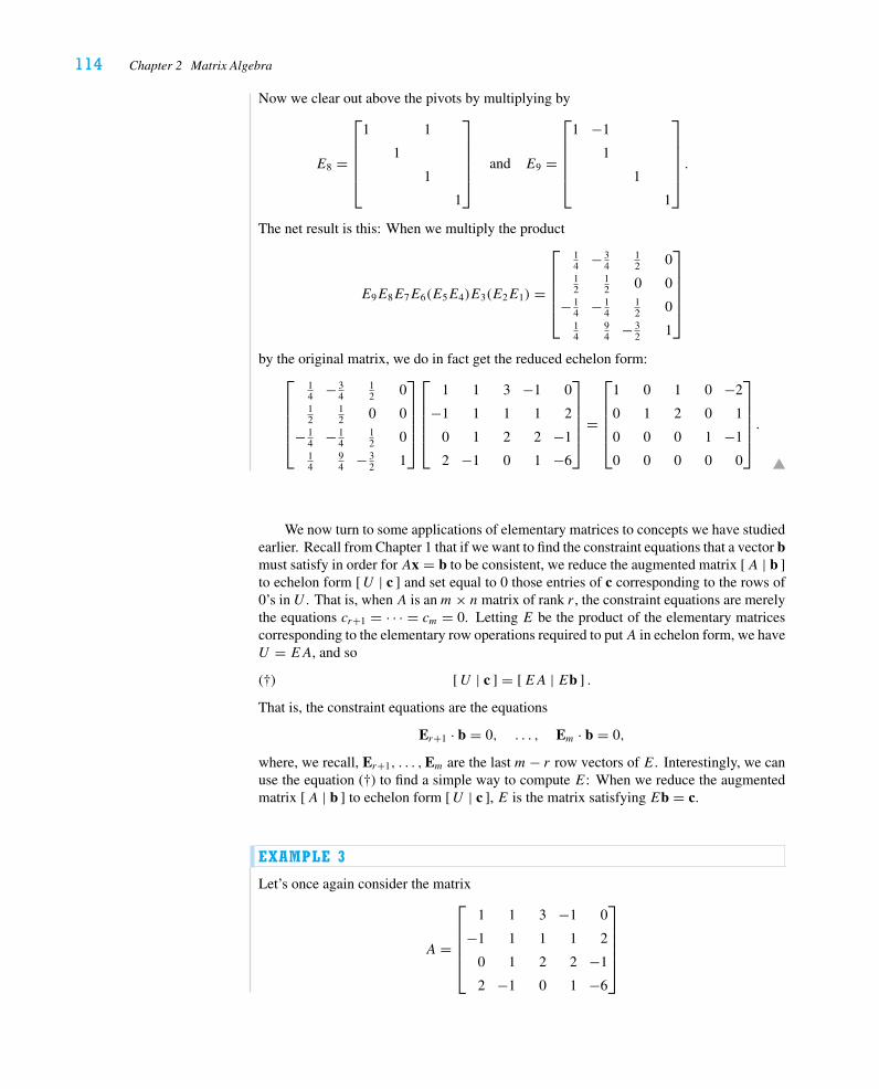
114 Chapter 2 Matrix Algebra
Now we clear out above the pivots by multiplying by
E8 =
⎡⎢⎢⎢⎢⎣
1 1
1
1
1
⎤⎥⎥⎥⎥⎦
and E9 =
⎡⎢⎢⎢⎢⎣
1 −1
1
1
1
⎤⎥⎥⎥⎥⎦.
The net result is this: When we multiply the product
E9E8E7E6(E5E4)E3(E2E1) =
⎡⎢⎢⎢⎢⎣
14 − 3
412 0
12
12 0 0
− 14 − 1
412 0
14
94 − 3
2 1
⎤⎥⎥⎥⎥⎦
by the original matrix, we do in fact get the reduced echelon form:⎡⎢⎢⎢⎢⎣
14 − 3
412 0
12
12 0 0
− 14 − 1
412 0
14
94 − 3
2 1
⎤⎥⎥⎥⎥⎦
⎡⎢⎢⎢⎢⎣
1 1 3 −1 0
−1 1 1 1 2
0 1 2 2 −1
2 −1 0 1 −6
⎤⎥⎥⎥⎥⎦
=
⎡⎢⎢⎢⎢⎣
1 0 1 0 −2
0 1 2 0 1
0 0 0 1 −1
0 0 0 0 0
⎤⎥⎥⎥⎥⎦.
We now turn to some applications of elementary matrices to concepts we have studiedearlier. Recall from Chapter 1 that if we want to find the constraint equations that a vector bmust satisfy in order for Ax = b to be consistent, we reduce the augmented matrix [A | b ]to echelon form [U | c ] and set equal to 0 those entries of c corresponding to the rows of0’s in U . That is, when A is anm× nmatrix of rank r , the constraint equations are merelythe equations cr+1 = · · · = cm = 0. Letting E be the product of the elementary matricescorresponding to the elementary row operations required to putA in echelon form, we haveU = EA, and so
(†) [U | c ] = [EA | Eb ] .
That is, the constraint equations are the equations
Er+1 · b = 0, . . . , Em · b = 0,
where, we recall, Er+1, . . . ,Em are the last m− r row vectors of E. Interestingly, we canuse the equation (†) to find a simple way to compute E: When we reduce the augmentedmatrix [A | b ] to echelon form [U | c ], E is the matrix satisfying Eb = c.
EXAMPLE 3
Let’s once again consider the matrix
A =
⎡⎢⎢⎢⎢⎣
1 1 3 −1 0
−1 1 1 1 2
0 1 2 2 −1
2 −1 0 1 −6
⎤⎥⎥⎥⎥⎦
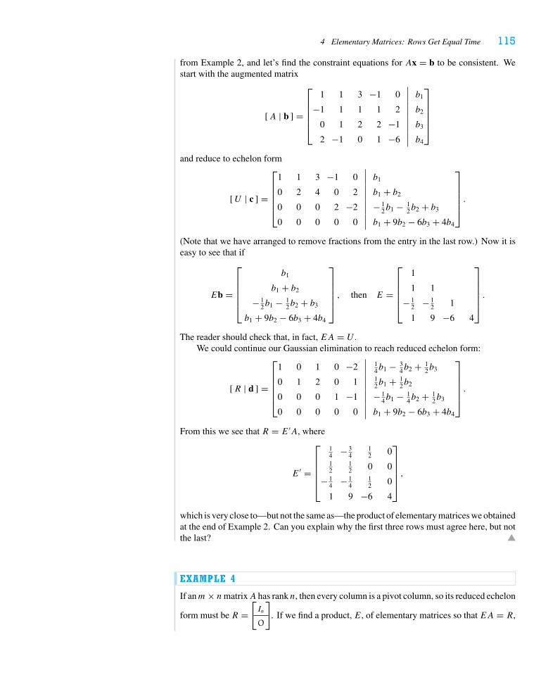
4 Elementary Matrices: Rows Get Equal Time 115
from Example 2, and let’s find the constraint equations for Ax = b to be consistent. Westart with the augmented matrix
[A | b ] =
⎡⎢⎢⎢⎢⎣
1 1 3 −1 0 b1
−1 1 1 1 2 b2
0 1 2 2 −1 b3
2 −1 0 1 −6 b4
⎤⎥⎥⎥⎥⎦
and reduce to echelon form
[U | c ] =
⎡⎢⎢⎢⎢⎣
1 1 3 −1 0 b1
0 2 4 0 2 b1 + b2
0 0 0 2 −2 − 12b1 − 1
2b2 + b3
0 0 0 0 0 b1 + 9b2 − 6b3 + 4b4
⎤⎥⎥⎥⎥⎦.
(Note that we have arranged to remove fractions from the entry in the last row.) Now it iseasy to see that if
Eb =
⎡⎢⎢⎢⎢⎣
b1
b1 + b2
− 12b1 − 1
2b2 + b3
b1 + 9b2 − 6b3 + 4b4
⎤⎥⎥⎥⎥⎦, then E =
⎡⎢⎢⎢⎢⎣
1
1 1
− 12 − 1
2 1
1 9 −6 4
⎤⎥⎥⎥⎥⎦.
The reader should check that, in fact, EA = U .We could continue our Gaussian elimination to reach reduced echelon form:
[R | d ] =
⎡⎢⎢⎢⎢⎣
1 0 1 0 −2 14b1 − 3
4b2 + 12b3
0 1 2 0 1 12b1 + 1
2b2
0 0 0 1 −1 − 14b1 − 1
4b2 + 12b3
0 0 0 0 0 b1 + 9b2 − 6b3 + 4b4
⎤⎥⎥⎥⎥⎦.
From this we see that R = E′A, where
E′ =
⎡⎢⎢⎢⎢⎣
14 − 3
412 0
12
12 0 0
− 14 − 1
412 0
1 9 −6 4
⎤⎥⎥⎥⎥⎦,
which is very close to—but not the same as—the product of elementary matrices we obtainedat the end of Example 2. Can you explain why the first three rows must agree here, but notthe last?
EXAMPLE 4
If anm× nmatrixA has rank n, then every column is a pivot column, so its reduced echelon
form must be R =[In
O
]. If we find a product, E, of elementary matrices so that EA = R,
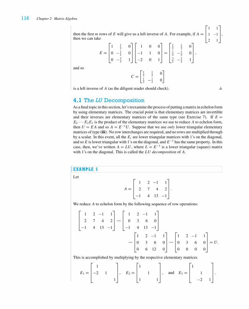
116 Chapter 2 Matrix Algebra
then the first m rows of E will give us a left inverse of A. For example, if A =⎡⎢⎣
1 1
1 −1
2 1
⎤⎥⎦,
then we can take
E =
⎡⎢⎢⎣
1 12 0
0 − 12 0
0 − 32 1
⎤⎥⎥⎦
⎡⎢⎢⎣
1 0 0
−1 1 0
−2 0 1
⎤⎥⎥⎦ =
⎡⎢⎢⎣
12
12 0
12 − 1
2 032 − 3
2 1
⎤⎥⎥⎦ ,
and so
C =[
12
12 0
12 − 1
2 0
]
is a left inverse of A (as the diligent reader should check).
4.1 The LU DecompositionAs a final topic in this section, let’s reexamine the process of putting a matrix in echelon formby using elementary matrices. The crucial point is that elementary matrices are invertibleand their inverses are elementary matrices of the same type (see Exercise 7). If E =Ek · · ·E2E1 is the product of the elementary matrices we use to reduce A to echelon form,then U = EA and so A = E−1U . Suppose that we use only lower triangular elementarymatrices of type (iii): No row interchanges are required, and no rows are multiplied throughby a scalar. In this event, all the Ei are lower triangular matrices with 1’s on the diagonal,and soE is lower triangular with 1’s on the diagonal, andE−1 has the same property. In thiscase, then, we’ve written A = LU , where L = E−1 is a lower triangular (square) matrixwith 1’s on the diagonal. This is called the LU decomposition of A.
EXAMPLE 5
Let
A =
⎡⎢⎢⎣
1 2 −1 1
2 7 4 2
−1 4 13 −1
⎤⎥⎥⎦ .
We reduce A to echelon form by the following sequence of row operations:⎡⎢⎢⎣
1 2 −1 1
2 7 4 2
−1 4 13 −1
⎤⎥⎥⎦�
⎡⎢⎢⎣
1 2 −1 1
0 3 6 0
−1 4 13 −1
⎤⎥⎥⎦
�
⎡⎢⎢⎣
1 2 −1 1
0 3 6 0
0 6 12 0
⎤⎥⎥⎦�
⎡⎢⎢⎣
1 2 −1 1
0 3 6 0
0 0 0 0
⎤⎥⎥⎦ = U.
This is accomplished by multiplying by the respective elementary matrices
E1 =
⎡⎢⎢⎣
1
−2 1
1
⎤⎥⎥⎦ , E2 =
⎡⎢⎢⎣
1
1
1 1
⎤⎥⎥⎦ , and E3 =
⎡⎢⎢⎣
1
1
−2 1
⎤⎥⎥⎦ .
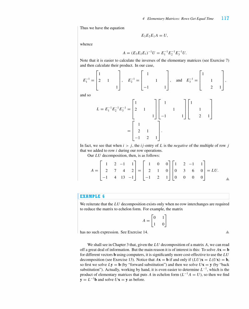
4 Elementary Matrices: Rows Get Equal Time 117
Thus we have the equation
E3E2E1A = U,
whence
A = (E3E2E1)−1U = E−1
1 E−12 E−1
3 U.
Note that it is easier to calculate the inverses of the elementary matrices (see Exercise 7)and then calculate their product. In our case,
E−11 =
⎡⎢⎢⎣
1
2 1
1
⎤⎥⎥⎦ , E−1
2 =
⎡⎢⎢⎣
1
1
−1 1
⎤⎥⎥⎦ , and E−1
3 =
⎡⎢⎢⎣
1
1
2 1
⎤⎥⎥⎦ ,
and so
L = E−11 E−1
2 E−13 =
⎡⎢⎢⎣
1
2 1
1
⎤⎥⎥⎦
⎡⎢⎢⎣
1
1
−1 1
⎤⎥⎥⎦
⎡⎢⎢⎣
1
1
2 1
⎤⎥⎥⎦
=
⎡⎢⎢⎣
1
2 1
−1 2 1
⎤⎥⎥⎦ .
In fact, we see that when i > j , the ij -entry of L is the negative of the multiple of row jthat we added to row i during our row operations.
Our LU decomposition, then, is as follows:
A =
⎡⎢⎢⎣
1 2 −1 1
2 7 4 2
−1 4 13 −1
⎤⎥⎥⎦ =
⎡⎢⎢⎣
1 0 0
2 1 0
−1 2 1
⎤⎥⎥⎦
⎡⎢⎢⎣
1 2 −1 1
0 3 6 0
0 0 0 0
⎤⎥⎥⎦ = LU.
EXAMPLE 6
We reiterate that the LU decomposition exists only when no row interchanges are requiredto reduce the matrix to echelon form. For example, the matrix
A =[
0 1
1 0
]
has no such expression. See Exercise 14.
We shall see in Chapter 3 that, given the LU decomposition of a matrixA, we can readoff a great deal of information. But the main reason it is of interest is this: To solveAx = bfor different vectors b using computers, it is significantly more cost-effective to use theLUdecomposition (see Exercise 13). Notice that Ax = b if and only if (LU)x = L(Ux) = b,so first we solve Ly = b (by “forward substitution”) and then we solve Ux = y (by “backsubstitution”). Actually, working by hand, it is even easier to determine L−1, which is theproduct of elementary matrices that puts A in echelon form (L−1A = U ), so then we findy = L−1b and solve Ux = y as before.
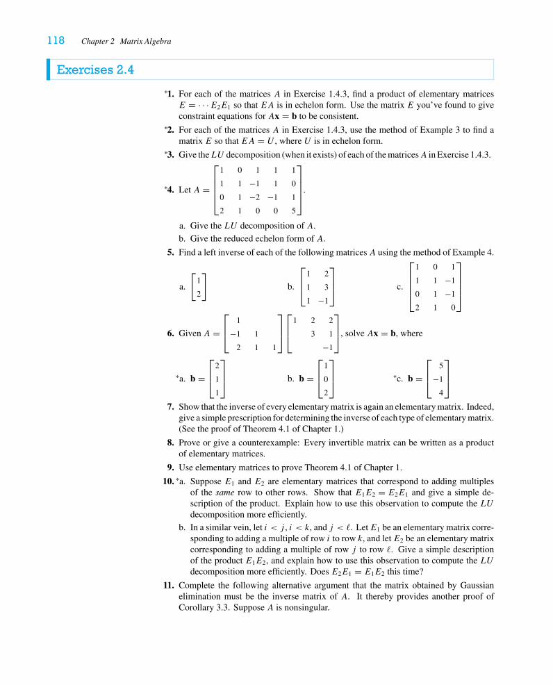
118 Chapter 2 Matrix Algebra
Exercises 2.4
1.∗ For each of the matrices A in Exercise 1.4.3, find a product of elementary matricesE = · · ·E2E1 so that EA is in echelon form. Use the matrix E you’ve found to giveconstraint equations for Ax = b to be consistent.
2.∗ For each of the matrices A in Exercise 1.4.3, use the method of Example 3 to find amatrix E so that EA = U , where U is in echelon form.
3.∗ Give theLU decomposition (when it exists) of each of the matricesA in Exercise 1.4.3.
4.∗ Let A =
⎡⎢⎢⎢⎣
1 0 1 1 1
1 1 −1 1 0
0 1 −2 −1 1
2 1 0 0 5
⎤⎥⎥⎥⎦.
a. Give the LU decomposition of A.
b. Give the reduced echelon form of A.
5. Find a left inverse of each of the following matricesA using the method of Example 4.
a.
[1
2
]b.
⎡⎢⎣
1 2
1 3
1 −1
⎤⎥⎦ c.
⎡⎢⎢⎢⎣
1 0 1
1 1 −1
0 1 −1
2 1 0
⎤⎥⎥⎥⎦
6. Given A =⎡⎢⎣
1
−1 1
2 1 1
⎤⎥⎦
⎡⎢⎣
1 2 2
3 1
−1
⎤⎥⎦, solve Ax = b, where
a.∗ b =⎡⎢⎣
2
1
1
⎤⎥⎦ b. b =
⎡⎢⎣
1
0
2
⎤⎥⎦ c.∗ b =
⎡⎢⎣
5
−1
4
⎤⎥⎦
7. Show that the inverse of every elementary matrix is again an elementary matrix. Indeed,give a simple prescription for determining the inverse of each type of elementary matrix.(See the proof of Theorem 4.1 of Chapter 1.)
8. Prove or give a counterexample: Every invertible matrix can be written as a productof elementary matrices.
9. Use elementary matrices to prove Theorem 4.1 of Chapter 1.
10. a.∗ Suppose E1 and E2 are elementary matrices that correspond to adding multiplesof the same row to other rows. Show that E1E2 = E2E1 and give a simple de-scription of the product. Explain how to use this observation to compute the LUdecomposition more efficiently.
b. In a similar vein, let i < j , i < k, and j < �. LetE1 be an elementary matrix corre-sponding to adding a multiple of row i to row k, and let E2 be an elementary matrixcorresponding to adding a multiple of row j to row �. Give a simple descriptionof the product E1E2, and explain how to use this observation to compute the LUdecomposition more efficiently. Does E2E1 = E1E2 this time?
11. Complete the following alternative argument that the matrix obtained by Gaussianelimination must be the inverse matrix of A. It thereby provides another proof ofCorollary 3.3. Suppose A is nonsingular.
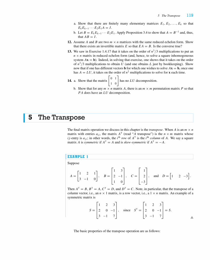
5 The Transpose 119
a. Show that there are finitely many elementary matrices E1, E2, . . . , Ek so thatEkEk−1 · · ·E2E1A = I .
b. Let B = EkEk−1 · · ·E2E1. Apply Proposition 3.4 to show that A = B−1 and, thus,that AB = I .
12. Assume A and B are two m× n matrices with the same reduced echelon form. Showthat there exists an invertible matrix E so that EA = B. Is the converse true?
13. We saw in Exercise 1.4.17 that it takes on the order of n3/3 multiplications to put ann× n matrix in reduced echelon form (and, hence, to solve a square inhomogeneoussystem Ax = b). Indeed, in solving that exercise, one shows that it takes on the orderof n3/3 multiplications to obtain U (and one obtains L just by bookkeeping). Shownow that if one has different vectors b for which one wishes to solveAx = b, once onehas A = LU , it takes on the order of n2 multiplications to solve for x each time.
14. a. Show that the matrix
[0 1
1 0
]has no LU decomposition.
b. Show that for anym× nmatrix A, there is anm×m permutation matrix P so thatPA does have an LU decomposition.
5 The Transpose
The final matrix operation we discuss in this chapter is the transpose. When A is anm× nmatrix with entries aij , the matrix AT (read “A transpose”) is the n×m matrix whoseij -entry is aji ; in other words, the i th row of AT is the i th column of A. We say a squarematrix A is symmetric if AT = A and is skew-symmetric if AT = −A.
EXAMPLE 1
Suppose
A =[
1 2 1
3 −1 0
], B =
⎡⎢⎢⎣
1 3
2 −1
1 0
⎤⎥⎥⎦ , C =
⎡⎢⎢⎣
1
2
−3
⎤⎥⎥⎦ , and D =
[1 2 −3
].
Then AT = B, BT = A, CT = D, and DT = C. Note, in particular, that the transpose of acolumn vector, i.e., an n× 1 matrix, is a row vector, i.e., a 1 × n matrix. An example of asymmetric matrix is
S =
⎡⎢⎢⎣
1 2 3
2 0 −1
3 −1 7
⎤⎥⎥⎦ , since ST =
⎡⎢⎢⎣
1 2 3
2 0 −1
3 −1 7
⎤⎥⎥⎦ = S.
The basic properties of the transpose operation are as follows:
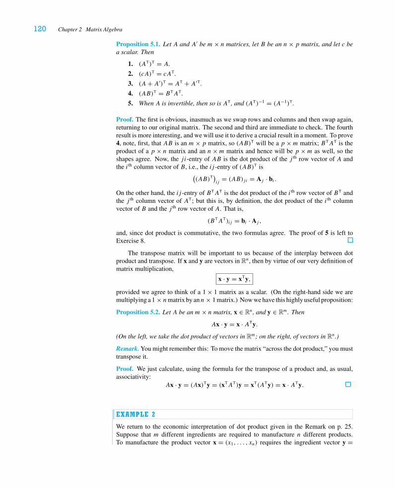
120 Chapter 2 Matrix Algebra
Proposition 5.1. Let A and A′ be m× n matrices, let B be an n× p matrix, and let c bea scalar. Then
1. (AT)T = A.
2. (cA)T = cAT.
3. (A+ A′)T = AT + A′T.
4. (AB)T = BTAT.
5. When A is invertible, then so is AT, and (AT)−1 = (A−1)T.
Proof. The first is obvious, inasmuch as we swap rows and columns and then swap again,returning to our original matrix. The second and third are immediate to check. The fourthresult is more interesting, and we will use it to derive a crucial result in a moment. To prove4, note, first, that AB is an m× p matrix, so (AB)T will be a p ×m matrix; BTAT is theproduct of a p × n matrix and an n×m matrix and hence will be p ×m as well, so theshapes agree. Now, the ji-entry of AB is the dot product of the j th row vector of A andthe i th column vector of B, i.e., the ij -entry of (AB)T is
((AB)T
)ij
= (AB)ji = Aj · bi .
On the other hand, the ij -entry of BTAT is the dot product of the i th row vector of BT andthe j th column vector of AT; but this is, by definition, the dot product of the i th columnvector of B and the j th row vector of A. That is,
(BTAT)ij = bi · Aj ,
and, since dot product is commutative, the two formulas agree. The proof of 5 is left toExercise 8.
The transpose matrix will be important to us because of the interplay between dotproduct and transpose. If x and y are vectors in Rn, then by virtue of our very definition ofmatrix multiplication,
x · y = xTy,
provided we agree to think of a 1 × 1 matrix as a scalar. (On the right-hand side we aremultiplying a 1 × nmatrix by ann× 1 matrix.) Now we have this highly useful proposition:
Proposition 5.2. Let A be an m× n matrix, x ∈ Rn, and y ∈ Rm. Then
Ax · y = x · ATy.
(On the left, we take the dot product of vectors in Rm; on the right, of vectors in Rn.)
Remark. You might remember this: To move the matrix “across the dot product,” you musttranspose it.
Proof. We just calculate, using the formula for the transpose of a product and, as usual,associativity:
Ax · y = (Ax)Ty = (xTAT)y = xT(ATy) = x · ATy.
EXAMPLE 2
We return to the economic interpretation of dot product given in the Remark on p. 25.Suppose that m different ingredients are required to manufacture n different products.To manufacture the product vector x = (x1, . . . , xn) requires the ingredient vector y =
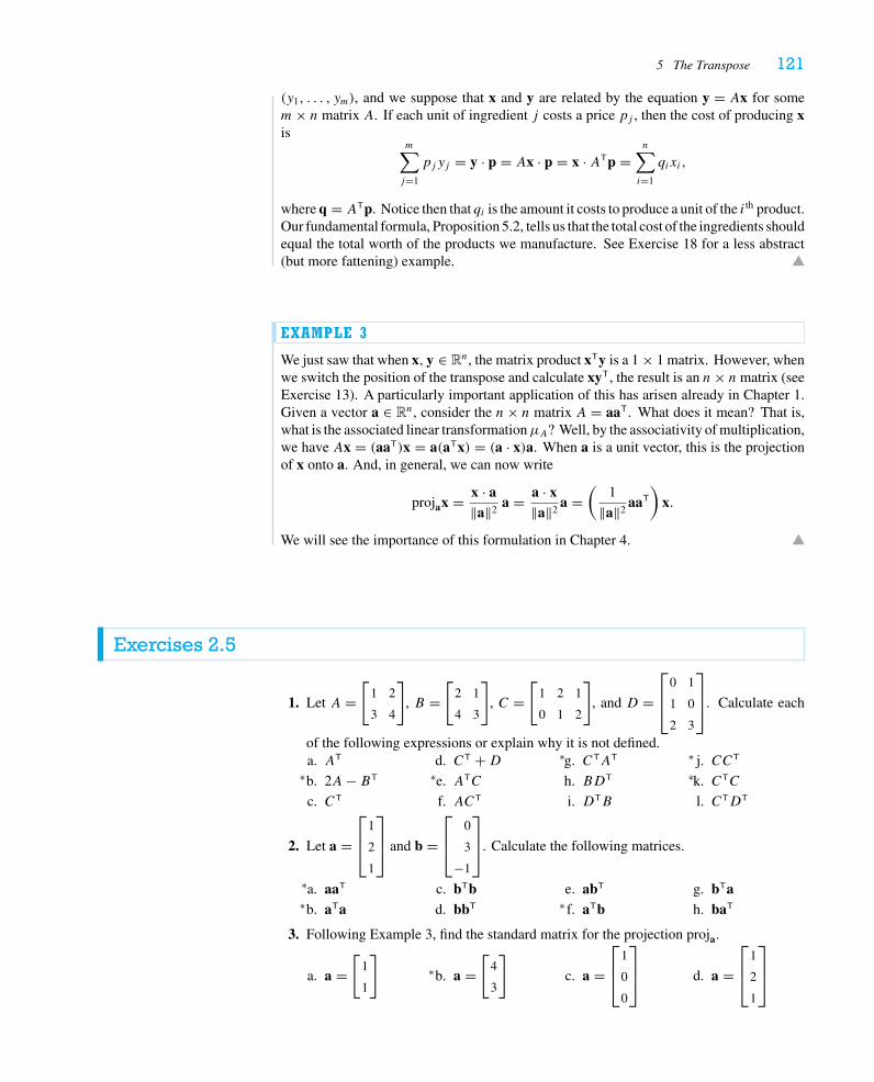
5 The Transpose 121
(y1, . . . , ym), and we suppose that x and y are related by the equation y = Ax for somem× n matrix A. If each unit of ingredient j costs a price pj , then the cost of producing xis
m∑j=1
pjyj = y · p = Ax · p = x · ATp =n∑i=1
qixi,
where q = ATp. Notice then that qi is the amount it costs to produce a unit of the i th product.Our fundamental formula, Proposition 5.2, tells us that the total cost of the ingredients shouldequal the total worth of the products we manufacture. See Exercise 18 for a less abstract(but more fattening) example.
EXAMPLE 3
We just saw that when x, y ∈ Rn, the matrix product xTy is a 1 × 1 matrix. However, whenwe switch the position of the transpose and calculate xyT, the result is an n× nmatrix (seeExercise 13). A particularly important application of this has arisen already in Chapter 1.Given a vector a ∈ Rn, consider the n× n matrix A = aaT. What does it mean? That is,what is the associated linear transformationμA? Well, by the associativity of multiplication,we have Ax = (aaT)x = a(aTx) = (a · x)a. When a is a unit vector, this is the projectionof x onto a. And, in general, we can now write
projax = x · a‖a‖2
a = a · x‖a‖2
a =(
1
‖a‖2aaT
)x.
We will see the importance of this formulation in Chapter 4.
Exercises 2.5
1. Let A =[
1 2
3 4
], B =
[2 1
4 3
], C =
[1 2 1
0 1 2
], and D =
⎡⎢⎣
0 1
1 0
2 3
⎤⎥⎦. Calculate each
of the following expressions or explain why it is not defined.a. AT
b.∗ 2A− BT
c. CT
d. CT +De.∗ ATC
f. ACT
g.∗ CTAT
h. BDT
i. DTB
j.∗ CCT
k.∗ CTC
l. CTDT
2. Let a =⎡⎢⎣
1
2
1
⎤⎥⎦ and b =
⎡⎢⎣
0
3
−1
⎤⎥⎦. Calculate the following matrices.
a.∗ aaT
b.∗ aTac. bTbd. bbT
e. abT
f.∗ aTbg. bTah. baT
3. Following Example 3, find the standard matrix for the projection proja.
a. a =[
1
1
]b.∗ a =
[4
3
]c. a =
⎡⎢⎣
1
0
0
⎤⎥⎦ d. a =
⎡⎢⎣
1
2
1
⎤⎥⎦
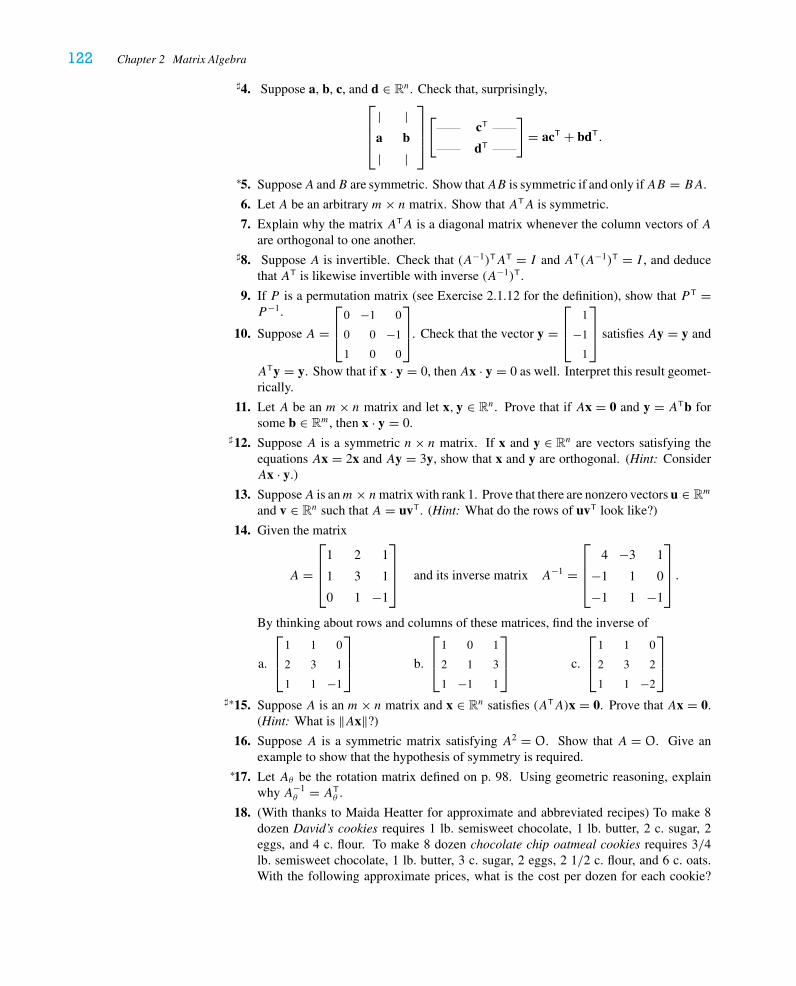
122 Chapter 2 Matrix Algebra
4.� Suppose a, b, c, and d ∈ Rn. Check that, surprisingly,⎡⎢⎢⎣
|a
|
|b
|
⎤⎥⎥⎦[
cT
dT
]= acT + bdT.
5.∗ SupposeA andB are symmetric. Show thatAB is symmetric if and only ifAB = BA.
6. Let A be an arbitrary m× n matrix. Show that ATA is symmetric.
7. Explain why the matrix ATA is a diagonal matrix whenever the column vectors of Aare orthogonal to one another.
8.� Suppose A is invertible. Check that (A−1)TAT = I and AT(A−1)T = I , and deducethat AT is likewise invertible with inverse (A−1)T.
9. If P is a permutation matrix (see Exercise 2.1.12 for the definition), show that P T =P−1.
10. Suppose A =⎡⎢⎣
0 −1 0
0 0 −1
1 0 0
⎤⎥⎦. Check that the vector y =
⎡⎢⎣
1
−1
1
⎤⎥⎦ satisfies Ay = y and
ATy = y. Show that if x · y = 0, then Ax · y = 0 as well. Interpret this result geomet-rically.
11. Let A be an m× n matrix and let x, y ∈ Rn. Prove that if Ax = 0 and y = ATb forsome b ∈ Rm, then x · y = 0.
12.� Suppose A is a symmetric n× n matrix. If x and y ∈ Rn are vectors satisfying theequations Ax = 2x and Ay = 3y, show that x and y are orthogonal. (Hint: ConsiderAx · y.)
13. SupposeA is anm× nmatrix with rank 1. Prove that there are nonzero vectors u ∈ Rm
and v ∈ Rn such that A = uvT. (Hint: What do the rows of uvT look like?)
14. Given the matrix
A =
⎡⎢⎢⎣
1 2 1
1 3 1
0 1 −1
⎤⎥⎥⎦ and its inverse matrix A−1 =
⎡⎢⎢⎣
4 −3 1
−1 1 0
−1 1 −1
⎤⎥⎥⎦ .
By thinking about rows and columns of these matrices, find the inverse of
a.
⎡⎢⎣
1 1 0
2 3 1
1 1 −1
⎤⎥⎦ b.
⎡⎢⎣
1 0 1
2 1 3
1 −1 1
⎤⎥⎦ c.
⎡⎢⎣
1 1 0
2 3 2
1 1 −2
⎤⎥⎦
15.�∗ Suppose A is an m× n matrix and x ∈ Rn satisfies (ATA)x = 0. Prove that Ax = 0.(Hint: What is ‖Ax‖?)
16. Suppose A is a symmetric matrix satisfying A2 = O. Show that A = O. Give anexample to show that the hypothesis of symmetry is required.
17.∗ Let Aθ be the rotation matrix defined on p. 98. Using geometric reasoning, explainwhy A−1
θ = ATθ .
18. (With thanks to Maida Heatter for approximate and abbreviated recipes) To make 8dozen David’s cookies requires 1 lb. semisweet chocolate, 1 lb. butter, 2 c. sugar, 2eggs, and 4 c. flour. To make 8 dozen chocolate chip oatmeal cookies requires 3/4lb. semisweet chocolate, 1 lb. butter, 3 c. sugar, 2 eggs, 2 1/2 c. flour, and 6 c. oats.With the following approximate prices, what is the cost per dozen for each cookie?
5 The Transpose 123
Use the approach of Example 2; what are the matrices A and AT?
Item Cost
1 lb. chocolate $4.80
1 lb. butter 3.40
1 c. sugar 0.20
1 dozen eggs 1.40
1 c. flour 0.10
1 c. oats 0.20
19.� We say an n× n matrix A is orthogonal if ATA = In.a. Prove that the column vectors a1, . . . , an of an orthogonal matrixA are unit vectors
that are orthogonal to one another, i.e.,
ai · aj ={
1, i = j
0, i �= j.
b. Fill in the missing columns in the following matrices to make them orthogonal:
[ √3
2 ?
− 12 ?
],
⎡⎢⎢⎣
1 0 ?
0 −1 ?
0 0 ?
⎤⎥⎥⎦ ,
⎡⎢⎢⎣
13 ? 2
323 ? − 2
323 ? 1
3
⎤⎥⎥⎦
c. Show that any 2 × 2 orthogonal matrix A must be of the form[
cos θ − sin θ
sin θ cos θ
]or
[cos θ sin θ
sin θ − cos θ
]
for some real number θ . (Hint: Use part a, rather than the original definition.)
d.∗ Show that ifA is an orthogonal 2 × 2 matrix, thenμA : R2 → R2 is either a rotationor the composition of a rotation and a reflection.
e. Prove that the row vectors A1, . . . ,An of an orthogonal matrix A are unit vectorsthat are orthogonal to one another. (Hint: Corollary 3.3.)
20. (Recall the definition of orthogonal matrices from Exercise 19.)a. Show that if A and B are orthogonal n× n matrices, then so is AB.
b.∗ Show that if A is an orthogonal matrix, then so is A−1.
21. Here is an alternative argument that when A is square and AB = I , it must be the casethat BA = I and so B = A−1.a. Suppose AB = I . Prove that AT is nonsingular. (Hint: Solve ATx = 0.)
b. Prove there exists a matrix C so that ATC = I , and hence CTA = I .
c. Use the result of part c of Exercise 2.1.11 to prove that B = A−1.
22.� a. Show that the only matrix that is both symmetric and skew-symmetric is O.
b. Given any square matrixA, show thatS = 12 (A+ AT) is symmetric andK = 1
2 (A−AT) is skew-symmetric.
c. Deduce that any square matrix A can be written in the form A = S +K , where Sis symmetric and K is skew-symmetric.
124 Chapter 2 Matrix Algebra
d. Prove that the expression in part c is unique: If A = S +K and A = S ′ +K ′(where S and S ′ are symmetric and K and K ′ are skew-symmetric), then S = S ′and K = K ′. (Hint: Use part a.)
(Recall the box on p. 91.) Remember also that to prove existence (in part c), youneed only find some S and K that work. There are really two different ways to proveuniqueness (in part d ). The route suggested in the problem is to suppose there weretwo different solutions and show they are really the same; an alternative is to deriveformulas for S and K , given the expression A = S +K .
23. a. Suppose A is an m× n matrix and Ax · y = 0 for every vector x ∈ Rn and everyvector y ∈ Rm. Prove that A = O.
b. Suppose A is a symmetric n× n matrix. Prove that if Ax · x = 0 for every vectorx ∈ Rn, then A = O. (Hint: Consider A(x + y) · (x + y).)
c. Give an example to show that the symmetry hypothesis is necessary in part b.
24. Suppose A is an n× n matrix satisfying Ax · y = x · Ay for all vectors x, y ∈ Rn.Prove that A is a symmetric matrix. (Hint: Show that (A− AT)x · y = 0 for allx, y ∈ Rn. Then use the result of part a of Exercise 23.)
HISTORICAL NOTESIn Chapter 1 we introduced matrices as a bookkeeping device for studying systems oflinear equations, whereas in this chapter the algebra of matrices has taken on a life of itsown, independent of any system of equations. Historically, the man who recognized theimportance of the algebra of matrices and unified the various fragments of this theory intoa subject worthy of standing by itself was Arthur Cayley (1821–1895).
Cayley was a British lawyer specializing in real estate law. He was successful butwas known to say that the law was a way for him to make money so that he could pursuehis true passion, mathematics. Indeed, he wrote almost 300 mathematics papers duringhis fourteen years of practicing law. Finally, in 1863, he sacrificed money for love andaccepted a professorship at Cambridge University. Of the many hundreds of mathematicspapers Cayley published during his career, the one of greatest interest here is his “Memoiron the Theory of Matrices,” which was published in 1858 while Cayley was still practicinglaw. It was in this work that Cayley defined much of what you have seen in this chapter.
The term matrix was coined by Cayley’s friend and colleague, James Joseph Sylvester(1814–1897). Many authors referred to what we now call a matrix as an “array” or “tableau.”Before its mathematical definition came along, the word matrix was used to describe “some-thing which surrounds, within which something is contained.” A perfect word for this newobject. The German mathematician F. G. Frobenius (1849–1917) had also been workingwith these structures, apparently without any knowledge of the work of Cayley and hiscolleagues. In 1878 he read Cayley’s “Memoir” and adopted the use of the word matrix.
Historical Notes 125
As for the notion of containment, Cayley was the first to delimit these arrays, bracketingthem to emphasize that a matrix was an object to be treated as a whole. Actually, Cayleyused an odd combination of curved and straight lines:
( r s t )
u v w
x y z
.
After introducing these objects, Cayley then defined addition, subtraction, and multiplica-tion and multiplicative inverse. Cayley’s study of matrices was initially motivated by thestudy of linear transformations. He considered matrices as defining transformations takingquantities (x, y, z) to new quantities (X, Y, Z), and he defined matrix multiplication bycomposing two such transformations, just as we did in Sections 1 and 2.
It may seem that the discovery of matrices and matrix algebra was a simple bit ofmathematics, but it helped lay a foundation on which a great deal of mathematics, appliedmathematics, and science has been built.

This page intentionally left blank
127
C H A P T E R 3VECTOR SPACES
We return now to elaborate on the geometric discussion of solutions of systems of linearequations initiated in Chapter 1. Because every solution of a homogeneous system of linearequations is given as a linear combination of vectors, we should view the sets of solutionsgeometrically as generalizations of lines, planes, and hyperplanes. Intuitively, lines andplanes differ in that it takes only one free variable (parameter) to describe points on aline (so a line is “one-dimensional”), but two to describe points on a plane (so a plane is“two-dimensional”). One of the goals of this chapter is to make algebraically precise thegeometric notion of dimension, so that we may assign a dimension to every subspace ofRn. Finally, at the end of this chapter, we shall see that these ideas extend far beyond therealm of Rn to the notion of an “abstract” vector space.
1 Subspaces of Rn
In Chapter 1 we learned to write the general solution of a system of linear equations instandard form; one consequence of this procedure is that it enables us to express the solutionset of a homogeneous system as the span of a particular set of vectors. The alert readerwill realize she learned one way of reversing this process in Chapter 1, and we will learnothers shortly. However, we should stop to understand that the span of a set of vectors inRn and the set of solutions of a homogeneous system of linear equations share some salientproperties.
Definition. A set V ⊂ Rn (a subset of Rn) is called a subspace of Rn if it satisfies allthe following properties:
1. 0 ∈ V (the zero vector belongs to V ).
2. Whenever v ∈ V and c ∈ R, we have cv ∈ V (V is closed under scalar multi-plication).
3. Whenever v,w ∈ V , we have v + w ∈ V (V is closed under addition).
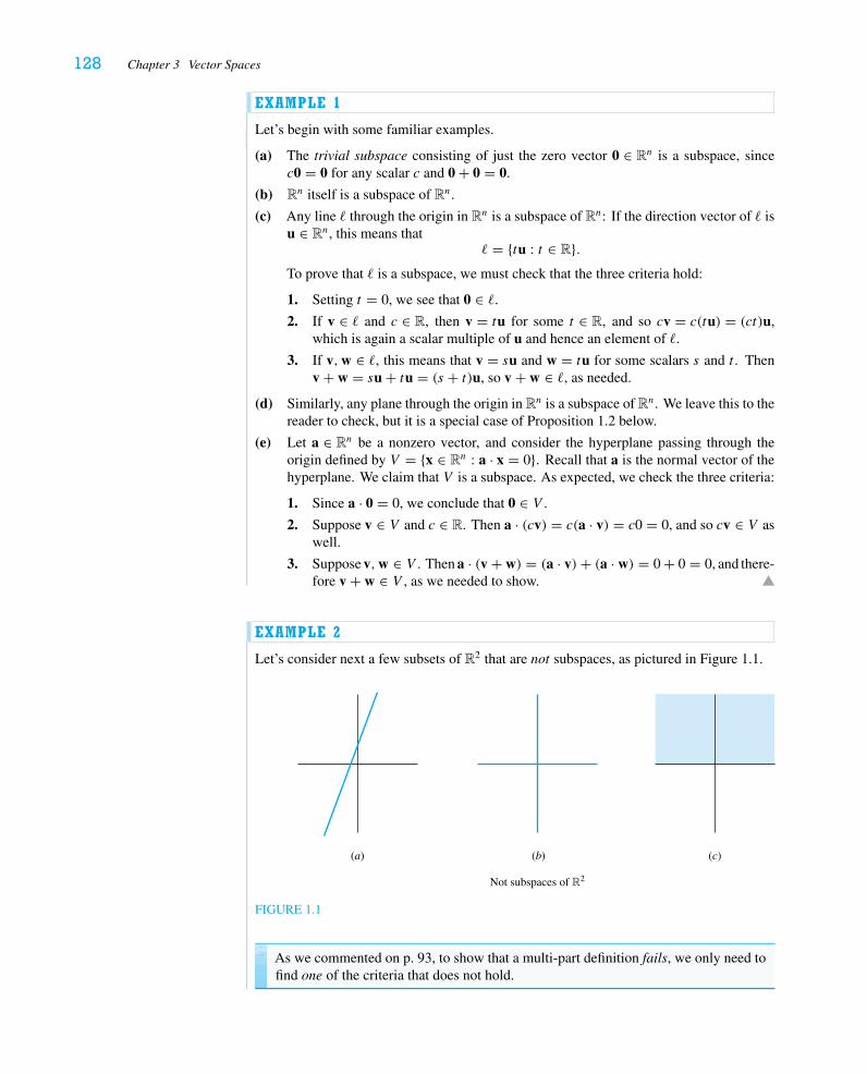
128 Chapter 3 Vector Spaces
EXAMPLE 1
Let’s begin with some familiar examples.
(a) The trivial subspace consisting of just the zero vector 0 ∈ Rn is a subspace, sincec0 = 0 for any scalar c and 0 + 0 = 0.
(b) Rn itself is a subspace of Rn.
(c) Any line � through the origin in Rn is a subspace of Rn: If the direction vector of � isu ∈ Rn, this means that
� = {tu : t ∈ R}.To prove that � is a subspace, we must check that the three criteria hold:
1. Setting t = 0, we see that 0 ∈ �.2. If v ∈ � and c ∈ R, then v = tu for some t ∈ R, and so cv = c(tu) = (ct)u,
which is again a scalar multiple of u and hence an element of �.
3. If v,w ∈ �, this means that v = su and w = tu for some scalars s and t . Thenv + w = su + tu = (s + t)u, so v + w ∈ �, as needed.
(d) Similarly, any plane through the origin in Rn is a subspace of Rn. We leave this to thereader to check, but it is a special case of Proposition 1.2 below.
(e) Let a ∈ Rn be a nonzero vector, and consider the hyperplane passing through theorigin defined by V = {x ∈ Rn : a · x = 0}. Recall that a is the normal vector of thehyperplane. We claim that V is a subspace. As expected, we check the three criteria:
1. Since a · 0 = 0, we conclude that 0 ∈ V .
2. Suppose v ∈ V and c ∈ R. Then a · (cv) = c(a · v) = c0 = 0, and so cv ∈ V aswell.
3. Suppose v,w ∈ V . Then a · (v + w) = (a · v)+ (a · w) = 0 + 0 = 0, and there-fore v + w ∈ V , as we needed to show.
EXAMPLE 2
Let’s consider next a few subsets of R2 that are not subspaces, as pictured in Figure 1.1.
(a) (b) (c)
Not subspaces of R2
FIGURE 1.1
As we commented on p. 93, to show that a multi-part definition fails, we only need tofind one of the criteria that does not hold.
1 Subspaces of Rn 129
(a) S = {(x1, x2) ∈ R2 : x2 = 2x1 + 1} is not a subspace. All three criteria fail, but itsuffices to point out 0 /∈ S.
(b) S = {(x1, x2) ∈ R2 : x1x2 = 0} is not a subspace. Each of the vectors v = (1, 0) andw = (0, 1) lies in S, and yet their sum v + w = (1, 1) does not.
(c) S = {(x1, x2) ∈ R2 : x2 ≥ 0} is not a subspace. The vector v = (0, 1) lies in S, andyet any negative scalar multiple of it, e.g., (−2)v = (0,−2), does not.
We now return to our motivating discussion. First, we consider the solution set of ahomogeneous linear system.
Proposition 1.1. Let A be an m× n matrix, and consider the set of solutions of thehomogeneous system of linear equations Ax = 0; that is, let
V = {x ∈ Rn : Ax = 0}.Then V is a subspace of Rn.
Proof. The proof is essentially the same as Example 1(e) if we think of the equationAx = 0as being the collection of equations A1 · x = A2 · x = · · · = Am · x = 0. But we wouldrather phrase the argument in terms of the linearity properties of matrix multiplication,discussed in Section 1 of Chapter 2.
As usual, we need only check that the three defining criteria all hold.
1. To check that 0 ∈ V , we recall thatA0 = 0, as a consequence of either of our waysof thinking of matrix multiplication.
2. If v ∈ V and c ∈ R, then we must show that cv ∈ V . Well, A(cv) = c(Av) =c0 = 0.
3. If v,w ∈ V , then we must show that v + w ∈ V . Since Av = Aw = 0, we haveA(v + w) = Av + Aw = 0 + 0 = 0, as required.
Thus, V is indeed a subspace of Rn.
Next, let v1, . . . , vk be vectors in Rn. In Chapter 1 we defined Span (v1, . . . , vk) to bethe set of all linear combinations of v1, . . . , vk; that is,
Span (v1, . . . , vk) = {v ∈ Rn : v = c1v1 + c2v2 + · · · + ckvk for some scalars c1, . . . , ck}.Generalizing what we observed in Examples 1(c) and (d), we have the following proposition.
Proposition 1.2. Let v1, . . . , vk ∈ Rn. Then V = Span (v1, . . . , vk) is a subspace of Rn.
Proof. We check that all three criteria hold.
1. To see that 0 ∈ V , we merely take c1 = c2 = · · · = ck = 0. Then c1v1 + c2v2 +· · · + ckvk = 0v1 + · · · + 0vk = 0 + · · · + 0 = 0.
2. Suppose v ∈ V and c ∈ R. By definition, there are scalars c1, . . . , ck so thatv = c1v1 + c2v2 + · · · + ckvk . Thus,
cv = c(c1v1 + c2v2 + · · · + ckvk) = (cc1)v1 + (cc2)v2 + · · · + (cck)vk,which is again a linear combination of v1, . . . , vk , so cv ∈ V , as desired.
3. Suppose v,w ∈ V . This means there are scalars c1, . . . , ck and d1, . . . , dk so that1
v = c1v1 + · · · + ckvk and w = d1v1 + · · · + dkvk;
1This might be a good time to review the content of the box following Exercise 1.1.22.
130 Chapter 3 Vector Spaces
adding, we obtain
v + w = (c1v1 + · · · + ckvk)+ (d1v1 + · · · + dkvk)= (c1 + d1)v1 + · · · + (ck + dk)vk,
which is again a linear combination of v1, . . . , vk and hence an element of V .
This completes the verification that V is a subspace of Rn.
Remark. Let V ⊂ Rn be a subspace and let v1, . . . , vk ∈ V . Then of course the subspaceSpan (v1, . . . , vk) is a subset ofV . We say that v1, . . . , vk spanV if Span (v1, . . . , vk) = V .(The point here is that every vector in V must be a linear combination of the vectorsv1, . . . , vk .)
EXAMPLE 3
The plane
P1 =
⎧⎪⎪⎨⎪⎪⎩s
⎡⎢⎢⎣
1
−1
2
⎤⎥⎥⎦+ t
⎡⎢⎢⎣
2
0
1
⎤⎥⎥⎦ : s, t ∈ R
⎫⎪⎪⎬⎪⎪⎭
is the span of the vectors
v1 =
⎡⎢⎢⎣
1
−1
2
⎤⎥⎥⎦ and v2 =
⎡⎢⎢⎣
2
0
1
⎤⎥⎥⎦
and is therefore a subspace of R3. On the other hand, the plane
P2 =
⎧⎪⎪⎨⎪⎪⎩
⎡⎢⎢⎣
1
0
0
⎤⎥⎥⎦+ s
⎡⎢⎢⎣
1
−1
2
⎤⎥⎥⎦+ t
⎡⎢⎢⎣
2
0
1
⎤⎥⎥⎦ : s, t ∈ R
⎫⎪⎪⎬⎪⎪⎭
is not a subspace. This is most easily verified by checking that 0 /∈ P2. Well, 0 ∈ P2
precisely when we can find values of s and t such that⎡⎢⎢⎣
0
0
0
⎤⎥⎥⎦ =
⎡⎢⎢⎣
1
0
0
⎤⎥⎥⎦+ s
⎡⎢⎢⎣
1
−1
2
⎤⎥⎥⎦+ t
⎡⎢⎢⎣
2
0
1
⎤⎥⎥⎦ .
This amounts to the system of equations
s + 2t = −1
−s = 0
2s + t = 0 ,
which we easily see is inconsistent.A word of warning here: We might have expressed P1 in the form
⎧⎪⎪⎨⎪⎪⎩
⎡⎢⎢⎣
1
1
−1
⎤⎥⎥⎦+ s
⎡⎢⎢⎣
1
−1
2
⎤⎥⎥⎦+ t
⎡⎢⎢⎣
2
0
1
⎤⎥⎥⎦ : s, t ∈ R
⎫⎪⎪⎬⎪⎪⎭
;
1 Subspaces of Rn 131
the presence of the “shifting” term may not prevent the plane from passing through theorigin.
EXAMPLE 4
Let
P1 = Span
⎛⎜⎜⎝
⎡⎢⎢⎣
1
0
0
⎤⎥⎥⎦ ,
⎡⎢⎢⎣
0
1
1
⎤⎥⎥⎦
⎞⎟⎟⎠ and P2 = Span
⎛⎜⎜⎝
⎡⎢⎢⎣
−1
1
0
⎤⎥⎥⎦ ,
⎡⎢⎢⎣
2
1
2
⎤⎥⎥⎦
⎞⎟⎟⎠ .
We wish to find all the vectors contained in both P1 and P2, i.e., the intersection P1 ∩ P2.A vector x lies in both P1 and P2 if and only if we can write x in both the forms
x = a
⎡⎢⎢⎣
1
0
0
⎤⎥⎥⎦+ b
⎡⎢⎢⎣
0
1
1
⎤⎥⎥⎦ and x = c
⎡⎢⎢⎣
−1
1
0
⎤⎥⎥⎦+ d
⎡⎢⎢⎣
2
1
2
⎤⎥⎥⎦
for some scalars a, b, c, and d. Setting the two expressions for x equal to one another andmoving all the vectors to one side, we obtain the system of equations
−a
⎡⎢⎢⎣
1
0
0
⎤⎥⎥⎦− b
⎡⎢⎢⎣
0
1
1
⎤⎥⎥⎦+ c
⎡⎢⎢⎣
−1
1
0
⎤⎥⎥⎦+ d
⎡⎢⎢⎣
2
1
2
⎤⎥⎥⎦ = 0.
In other words, we want to find all solutions of the system
⎡⎢⎢⎣
1 0 −1 2
0 1 1 1
0 1 0 2
⎤⎥⎥⎦
⎡⎢⎢⎢⎢⎣
−a−bc
d
⎤⎥⎥⎥⎥⎦
= 0,
and so we reduce the matrix
A =
⎡⎢⎢⎣
1 0 −1 2
0 1 1 1
0 1 0 2
⎤⎥⎥⎦
to reduced echelon form
R =
⎡⎢⎢⎣
1 0 0 1
0 1 0 2
0 0 1 −1
⎤⎥⎥⎦
and find that every solution of Ay = 0 is a scalar multiple of the vector⎡⎢⎢⎢⎢⎣
−a−bc
d
⎤⎥⎥⎥⎥⎦
=
⎡⎢⎢⎢⎢⎣
−1
−2
1
1
⎤⎥⎥⎥⎥⎦.
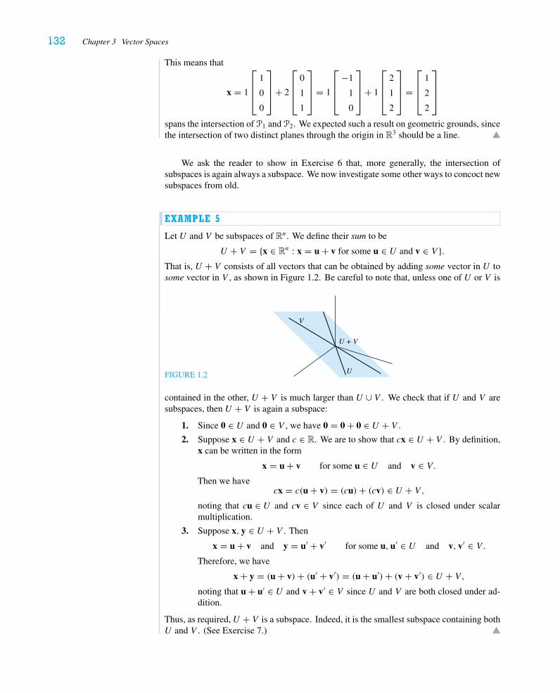
132 Chapter 3 Vector Spaces
This means that
x = 1
⎡⎢⎢⎣
1
0
0
⎤⎥⎥⎦+ 2
⎡⎢⎢⎣
0
1
1
⎤⎥⎥⎦ = 1
⎡⎢⎢⎣
−1
1
0
⎤⎥⎥⎦+ 1
⎡⎢⎢⎣
2
1
2
⎤⎥⎥⎦ =
⎡⎢⎢⎣
1
2
2
⎤⎥⎥⎦
spans the intersection of P1 and P2. We expected such a result on geometric grounds, sincethe intersection of two distinct planes through the origin in R3 should be a line.
We ask the reader to show in Exercise 6 that, more generally, the intersection ofsubspaces is again always a subspace. We now investigate some other ways to concoct newsubspaces from old.
EXAMPLE 5
Let U and V be subspaces of Rn. We define their sum to be
U + V = {x ∈ Rn : x = u + v for some u ∈ U and v ∈ V }.That is, U + V consists of all vectors that can be obtained by adding some vector in U tosome vector in V , as shown in Figure 1.2. Be careful to note that, unless one of U or V is
FIGURE 1.2
V
U
U + V
contained in the other, U + V is much larger than U ∪ V . We check that if U and V aresubspaces, then U + V is again a subspace:
1. Since 0 ∈ U and 0 ∈ V , we have 0 = 0 + 0 ∈ U + V .
2. Suppose x ∈ U + V and c ∈ R. We are to show that cx ∈ U + V . By definition,x can be written in the form
x = u + v for some u ∈ U and v ∈ V.Then we have
cx = c(u + v) = (cu)+ (cv) ∈ U + V,noting that cu ∈ U and cv ∈ V since each of U and V is closed under scalarmultiplication.
3. Suppose x, y ∈ U + V . Then
x = u + v and y = u′ + v′ for some u, u′ ∈ U and v, v′ ∈ V.Therefore, we have
x + y = (u + v)+ (u′ + v′) = (u + u′)+ (v + v′) ∈ U + V,noting that u + u′ ∈ U and v + v′ ∈ V since U and V are both closed under ad-dition.
Thus, as required, U + V is a subspace. Indeed, it is the smallest subspace containing bothU and V . (See Exercise 7.)
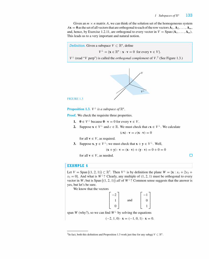
1 Subspaces of Rn 133
Given anm× nmatrixA, we can think of the solution set of the homogeneous systemAx = 0 as the set of all vectors that are orthogonal to each of the row vectors A1,A2, . . . ,Am,and, hence, by Exercise 1.2.11, are orthogonal to every vector in V = Span (A1, . . . ,Am).This leads us to a very important and natural notion.
Definition. Given a subspace V ⊂ Rn, define
V ⊥ = {x ∈ Rn : x · v = 0 for every v ∈ V }.V ⊥ (read “V perp”) is called the orthogonal complement of V .2 (See Figure 1.3.)
FIGURE 1.3
V
V⊥
Proposition 1.3. V ⊥ is a subspace of Rn.
Proof. We check the requisite three properties.
1. 0 ∈ V ⊥ because 0 · v = 0 for every v ∈ V .
2. Suppose x ∈ V ⊥ and c ∈ R. We must check that cx ∈ V ⊥. We calculate
(cx) · v = c(x · v) = 0
for all v ∈ V , as required.
3. Suppose x, y ∈ V ⊥; we must check that x + y ∈ V ⊥. Well,
(x + y) · v = (x · v)+ (y · v) = 0 + 0 = 0
for all v ∈ V , as needed.
EXAMPLE 6
Let V = Span((1, 2, 1)
) ⊂ R3. Then V ⊥ is by definition the plane W = {x : x1 + 2x2 +x3 = 0}. And what is W⊥? Clearly, any multiple of (1, 2, 1) must be orthogonal to everyvector inW ; but is Span
((1, 2, 1)
)all ofW⊥? Common sense suggests that the answer is
yes, but let’s be sure.We know that the vectors⎡
⎢⎢⎣−2
1
0
⎤⎥⎥⎦ and
⎡⎢⎢⎣
−1
0
1
⎤⎥⎥⎦
spanW (why?), so we can findW⊥ by solving the equations
(−2, 1, 0) · x = (−1, 0, 1) · x = 0.
2In fact, both this definition and Proposition 1.3 work just fine for any subset V ⊂ Rn.
134 Chapter 3 Vector Spaces
By finding the reduced echelon form of the coefficient matrix
A =[−2 1 0
−1 0 1
]�[
1 0 −1
0 1 −2
],
we see that, indeed, every vector inW⊥ is a multiple of (1, 2, 1), as we suspected.
It is extremely important to observe that if c ∈ V ⊥, then all the elements of V satisfythe linear equation c · x = 0. Thus, there is an intimate relation between elements of V ⊥and Cartesian equations defining the subspace V . We will explore and exploit this relationmore fully in the next few sections.
It will be useful for us to make the following definition.
Definition. LetV andW be subspaces of Rn. We sayV andW are orthogonal subspacesif every element of V is orthogonal to every element ofW , i.e., if
v · w = 0 for every v ∈ V and every w ∈ W.
Remark. If V = W⊥ or W = V ⊥, then clearly V and W are orthogonal subspaces. Onthe other hand, if V and W are orthogonal subspaces of Rn, then certainly W ⊂ V ⊥ andV ⊂ W⊥. (See Exercise 12.) Of course, W need not be equal to V ⊥: Consider, forexample, V to be the x1-axis and W to be the x2-axis in R3. Then V ⊥ is the x2x3-plane,which contains W and more. It is natural, however, to ask the following question: IfW = V ⊥, must V = W⊥? We will return to this shortly.
Exercises 3.1
1.∗ Which of the following are subspaces? Justify your answer in each case.a. {x ∈ R2 : x1 + x2 = 1}
b. {x ∈ R3 : x =⎡⎢⎣
a
b
a + b
⎤⎥⎦ for some a, b ∈ R}
c. {x ∈ R3 : x1 + 2x2 < 0}d. {x ∈ R3 : x2
1 + x22 + x2
3 = 1}e. {x ∈ R3 : x2
1 + x22 + x2
3 = 0}f. {x ∈ R3 : x2
1 + x22 + x2
3 = −1}
g. {x ∈ R3 : x = s
⎡⎢⎣
2
1
1
⎤⎥⎦+ t
⎡⎢⎣
1
2
1
⎤⎥⎦ for some s, t ∈ R}
h. {x ∈ R3 : x =⎡⎢⎣
3
0
1
⎤⎥⎦+ s
⎡⎢⎣
2
1
1
⎤⎥⎦+ t
⎡⎢⎣
1
2
1
⎤⎥⎦ for some s, t ∈ R}
i. {x ∈ R3 : x =⎡⎢⎣
2
4
−1
⎤⎥⎦+ s
⎡⎢⎣
2
1
1
⎤⎥⎦+ t
⎡⎢⎣
1
2
−1
⎤⎥⎦ for some s, t ∈ R}
1 Subspaces of Rn 135
2.∗ Decide whether each of the following collections of vectors spans R3.a. (1, 1, 1), (1, 2, 2)
b. (1, 1, 1), (1, 2, 2), (1, 3, 3)
c. (1, 0, 1), (1,−1, 1), (3, 5, 3), (2, 3, 2)
d. (1, 0,−1), (2, 1, 1), (0, 1, 5)
3.∗ Criticize the following argument: For any vector v, we have 0v = 0. So the firstcriterion for subspaces is, in fact, a consequence of the second criterion and couldtherefore be omitted.
4. Let A be an n× n matrix. Verify that
V = {x ∈ Rn : Ax = 3x}is a subspace of Rn.
5. Let A and B be m× n matrices. Show that
V = {x ∈ Rn : Ax = Bx}is a subspace of Rn.
6. a. Let U and V be subspaces of Rn. Define the intersection of U and V to be
U ∩ V = {x ∈ Rn : x ∈ U and x ∈ V }.Show that U ∩ V is a subspace of Rn. Give two examples.
b. Is U ∪ V = {x ∈ Rn : x ∈ U or x ∈ V } always a subspace of Rn? Give a proof orcounterexample.
7. Prove that ifU and V are subspaces of Rn andW is a subspace of Rn containing all thevectors of U and all the vectors of V (that is, U ⊂ W and V ⊂ W ), then U + V ⊂ W .This means that U + V is the smallest subspace containing both U and V .
8. Let v1, . . . , vk ∈ Rn and let v ∈ Rn. Prove that
Span (v1, . . . , vk) = Span (v1, . . . , vk, v) if and only if v ∈ Span (v1, . . . , vk).
9. Determine the intersection of the subspaces P1 and P2 in each case:a.∗ P1 = Span
((1, 0, 1), (2, 1, 2)
), P2 = Span
((1,−1, 0), (1, 3, 2)
)b. P1 = Span
((1, 2, 2), (0, 1, 1)
), P2 = Span
((2, 1, 1), (1, 0, 0)
)c. P1 = Span
((1, 0,−1), (1, 2, 3)
), P2 = {x : x1 − x2 + x3 = 0}
d.∗ P1 = Span((1, 1, 0, 1), (0, 1, 1, 0)
), P2 = Span
((0, 0, 1, 1), (1, 1, 0, 0)
)e. P1 = Span
((1, 0, 1, 2), (0, 1, 0,−1)
), P2 = Span
((1, 1, 2, 1), (1, 1, 0, 1)
)
10.�∗ Let V ⊂ Rn be a subspace. Show that V ∩ V ⊥ = {0}.11. Suppose V andW are orthogonal subspaces of Rn, i.e., v · w = 0 for every v ∈ V and
every w ∈ W . Prove that V ∩W = {0}.12.�∗ Suppose V andW are orthogonal subspaces of Rn, i.e., v · w = 0 for every v ∈ V and
every w ∈ W . Prove that V ⊂ W⊥.
13.� Let V ⊂ Rn be a subspace. Show that V ⊂ (V ⊥)⊥. Do you think more is true?
14.� Let V andW be subspaces of Rn with the property that V ⊂ W . Prove thatW⊥ ⊂ V ⊥.
15. Let A be an m× n matrix. Let V ⊂ Rn andW ⊂ Rm be subspaces.a. Show that {x ∈ Rn : Ax ∈ W } is a subspace of Rn.
b. Show that {y ∈ Rm : y = Ax for some x ∈ V } is a subspace of Rm.
16. Suppose A is a symmetric n× n matrix. Let V ⊂ Rn be a subspace with the propertythat Ax ∈ V for every x ∈ V . Show that Ay ∈ V ⊥ for all y ∈ V ⊥.
17. Use Exercises 13 and 14 to prove that for any subspace V ⊂ Rn, we have V ⊥ =((V ⊥)⊥
)⊥.
18. Suppose U and V are subspaces of Rn. Prove that (U + V )⊥ = U⊥ ∩ V ⊥.
136 Chapter 3 Vector Spaces
2 The Four Fundamental Subspaces
As we have seen, two of the most important constructions we’ve studied in linear algebra—the span of a collection of vectors and the set of solutions of a homogeneous linear systemof equations—lead to subspaces. Let’s use these notions to define four important subspacesassociated to an m× n matrix.
The first two are already quite familiar to us from our work in Chapter 1, and we haveseen in Section 1 of this chapter that they are in fact subspaces. Here we will give themtheir official names.
Definition (Nullspace). Let A be an m× n matrix. The nullspace of A is the set ofsolutions of the homogeneous system Ax = 0:
N(A) = {x ∈ Rn : Ax = 0}.
Definition (Column Space). Let A be an m× n matrix with column vectors a1, . . . ,
an ∈ Rm. We define the column space of A to be the subspace of Rm spanned by thecolumn vectors:
C(A) = Span (a1, . . . , an) ⊂ Rm.
Of course, the nullspace, N(A), is just the set of solutions of the homogeneous linearsystem Ax = 0 that we first encountered in Section 4 of Chapter 1. What is less obvious isthat we encountered the column space, C(A), in Section 5 of Chapter 1, as we now see.
Proposition 2.1. Let A be an m× n matrix. Let b ∈ Rm. Then b ∈ C(A) if and only ifb = Ax for some x ∈ Rn. That is,
C(A) = {b ∈ Rm : Ax = b is consistent}.
Proof. By definition, C(A) = Span (a1, . . . , an), and so b ∈ C(A) if and only if b is alinear combination of the vectors a1, . . . , an; i.e., b = x1a1 + · · · + xnan for some scalarsx1, . . . , xn. Recalling our crucial observation (∗) on p. 53, we conclude that b ∈ C(A) ifand only if b = Ax for some x ∈ Rn. The final reformulation is straightforward so long aswe remember that the system Ax = b is consistent provided it has a solution.
Remark. If, as in Section 1 of Chapter 2, we think ofA as giving a functionμA : Rn → Rm,then C(A) ⊂ Rm is the set of all the values of the function μA, i.e., the image of μA. Itis important to keep track of where each subspace “lives” as you continue through thischapter: The nullspace N(A) consists of x’s (inputs of μA) and is a subspace of Rn; thecolumn space C(A) consists of b’s (outputs of the function μA) and is a subspace of Rm.
A theme we explored in Chapter 1 was that lines and planes can be described eitherparametrically or by Cartesian equations. This idea should work for general subspaces ofRn. We give a parametric description of a subspace V when we describe V as the span ofvectors v1, . . . , vk . Putting these vectors as the columns of a matrix A amounts to writingV = C(A). Similarly, giving Cartesian equations forV , once we translate them into matrix
2 The Four Fundamental Subspaces 137
form, is giving V = N(A) for the appropriate matrix A.3 Much of Sections 4 and 5 ofChapter 1 was devoted to going from one description to the other: In our present language,by finding the general solution of Ax = 0, we obtain a parametric description of N(A)and thus obtain vectors that span that subspace. On the other hand, finding the constraintequations for Ax = b to be consistent provides a set of Cartesian equations for C(A).
EXAMPLE 1
Let
A =
⎡⎢⎢⎣
1 −1 1 2
1 0 1 1
1 2 1 −1
⎤⎥⎥⎦ .
Of course, we bring A to its reduced echelon form
R =
⎡⎢⎢⎣
1 0 1 1
0 1 0 −1
0 0 0 0
⎤⎥⎥⎦
and read off the general solution of Ax = 0:
x1 = −x3 − x4
x2 = x4
x3 = x3
x4 = x4 ,
that is,
x =
⎡⎢⎢⎢⎢⎣
x1
x2
x3
x4
⎤⎥⎥⎥⎥⎦
=
⎡⎢⎢⎢⎢⎣
−x3−x4
x4
x3
x4
⎤⎥⎥⎥⎥⎦
= x3
⎡⎢⎢⎢⎢⎣
−1
0
1
0
⎤⎥⎥⎥⎥⎦
+ x4
⎡⎢⎢⎢⎢⎣
−1
1
0
1
⎤⎥⎥⎥⎥⎦.
From this we see that the vectors
v1 =
⎡⎢⎢⎢⎢⎣
−1
0
1
0
⎤⎥⎥⎥⎥⎦
and v2 =
⎡⎢⎢⎢⎢⎣
−1
1
0
1
⎤⎥⎥⎥⎥⎦
span N(A).
On other hand, we know that the vectors
⎡⎢⎣
1
1
1
⎤⎥⎦,
⎡⎢⎣
−1
0
2
⎤⎥⎦, and
⎡⎢⎣
2
1
−1
⎤⎥⎦ span C(A). To find
Cartesian equations for C(A), we find the constraint equations for Ax = b to be consistent
3The astute reader may be worried that we have not yet shown that every subspace can be described in eithermanner. We will address this matter in Section 4.
138 Chapter 3 Vector Spaces
by reducing the augmented matrix⎡⎢⎢⎣
1 −1 1 2 b1
1 0 1 1 b2
1 2 1 −1 b3
⎤⎥⎥⎦ �
⎡⎢⎢⎣
1 −1 1 2 b1
0 1 0 −1 b2 − b1
0 0 0 0 2b1 − 3b2 + b3
⎤⎥⎥⎦ ,
from which we see that 2b1 − 3b2 + b3 = 0 gives a Cartesian description of C(A). Ofcourse, we might want to replace b’s with x’s and just write
C(A) = {x ∈ R3 : 2x1 − 3x2 + x3 = 0}.We can summarize these results by defining new matrices
X =
⎡⎢⎢⎢⎢⎣
−1 −1
0 1
1 0
0 1
⎤⎥⎥⎥⎥⎦
and Y =[2 −3 1
],
and then we have N(A) = C(X) and C(A) = N(Y ). One final remark: Note that thecoefficients of the constraint equation(s), i.e., the row(s) of Y , give vectors orthogonal toC(A), just as the rows of A are orthogonal to N(A) (and hence to the columns of X).
We now move on to discuss the last two of the four subspaces associated to the matrixA. In the interest of fair play, since we’ve already dedicated a subspace to the columns ofA, it is natural to make the following definition.
Definition (RowSpace). LetA be anm× nmatrix with row vectors A1, . . . ,Am ∈ Rn.We define the row space of A to be the subspace of Rn spanned by the row vectorsA1, . . . ,Am:
R(A) = Span (A1, . . . ,Am) ⊂ Rn.
It is important to remember that, as vectors in Rn, the Ai are still represented by columnvectors with n entries. But we continue our practice of writing vectors in parentheses whenit is typographically more convenient.
Noting that R(A) = C(AT), it is natural then to complete the quartet as follows:
Definition (Left Nullspace). We define the left nullspace of the m× n matrix A to be
N(AT) = {x ∈ Rm : ATx = 0} = {x ∈ Rm : xTA = 0T}.(The latter description accounts for the terminology.)
Just as elements of the nullspace of A give us the linear combinations of the columnvectors of A that result in the zero vector, elements of the left nullspace give us the linearcombinations of the row vectors of A that result in zero.
Once again, we pause to remark on the “locations” of the subspaces. N(A) and R(A)are “neighbors,” both being subspaces of Rn (the domain of the linear map μA). C(A) andN(AT) are “neighbors” in Rm, the range of μA and the domain of μAT . We will soon havea more complete picture of the situation.
In the discussion leading up to Proposition 1.3 we observed that vectors in the nullspaceofA are orthogonal to all the row vectors ofA—that is, that N(A) and R(A) are orthogonal
2 The Four Fundamental Subspaces 139
subspaces. In fact, the orthogonality relations among our “neighboring” subspaces willprovide a lot of information about linear maps. We begin with the following proposition.
Proposition 2.2. Let A be an m× n matrix. Then N(A) = R(A)⊥.
Proof. If x ∈ N(A), then x is orthogonal to each row vector A1, . . . ,Am ofA. By Exercise1.2.11, x is orthogonal to every vector in R(A) and is therefore an element of R(A)⊥. Thus,N(A) is a subset of R(A)⊥, and so we need only show that R(A)⊥ is a subset of N(A).(Recall the box on p. 12.) If x ∈ R(A)⊥, this means that x is orthogonal to every vectorin R(A), so, in particular, x is orthogonal to each of the row vectors A1, . . . ,Am. But thismeans that Ax = 0, so x ∈ N(A), as required.
Since C(A) = R(AT), when we substituteAT forA the following result is an immediateconsequence of Proposition 2.2.
Proposition 2.3. Let A be an m× n matrix. Then N(AT) = C(A)⊥.
Proposition 2.3 has a very pleasant interpretation in terms of the constraint equationsfor Ax = b to be consistent—the Cartesian equations for C(A). As we commented inSection 1, the coefficients of such a Cartesian equation give a vector orthogonal to C(A),i.e., an element of C(A)⊥ = N(AT). Thus, a constraint equation gives a linear combinationof the rows that results in the zero vector. But, of course, this is where constraint equationscome from in the first place. Conversely, any such relation among the row vectors of Agives an element of N(AT) = C(A)⊥, and hence the coefficients of a constraint equationthat b must satisfy in order for Ax = b to be consistent.
EXAMPLE 2
Let
A =
⎡⎢⎢⎢⎢⎣
1 2
1 1
0 1
1 2
⎤⎥⎥⎥⎥⎦.
We find the constraint equations forAx = b to be consistent by row reducing the augmentedmatrix:⎡
⎢⎢⎢⎢⎣
1 2 b1
1 1 b2
0 1 b3
1 2 b4
⎤⎥⎥⎥⎥⎦
�
⎡⎢⎢⎢⎢⎣
1 2 b1
0 −1 b2 − b1
0 1 b3
0 0 b4 − b1
⎤⎥⎥⎥⎥⎦
�
⎡⎢⎢⎢⎢⎣
1 2 b1
0 1 b1 − b2
0 0 −b1 + b2 + b3
0 0 −b1 + b4
⎤⎥⎥⎥⎥⎦.
The constraint equations are
−b1 + b2 + b3 = 0
−b1 + b4 = 0 .
Note that the vectors
c1 =
⎡⎢⎢⎢⎢⎣
−1
1
1
0
⎤⎥⎥⎥⎥⎦
and c2 =
⎡⎢⎢⎢⎢⎣
−1
0
0
1
⎤⎥⎥⎥⎥⎦
are in N(AT) and correspond to linear combinations of the rows yielding 0.
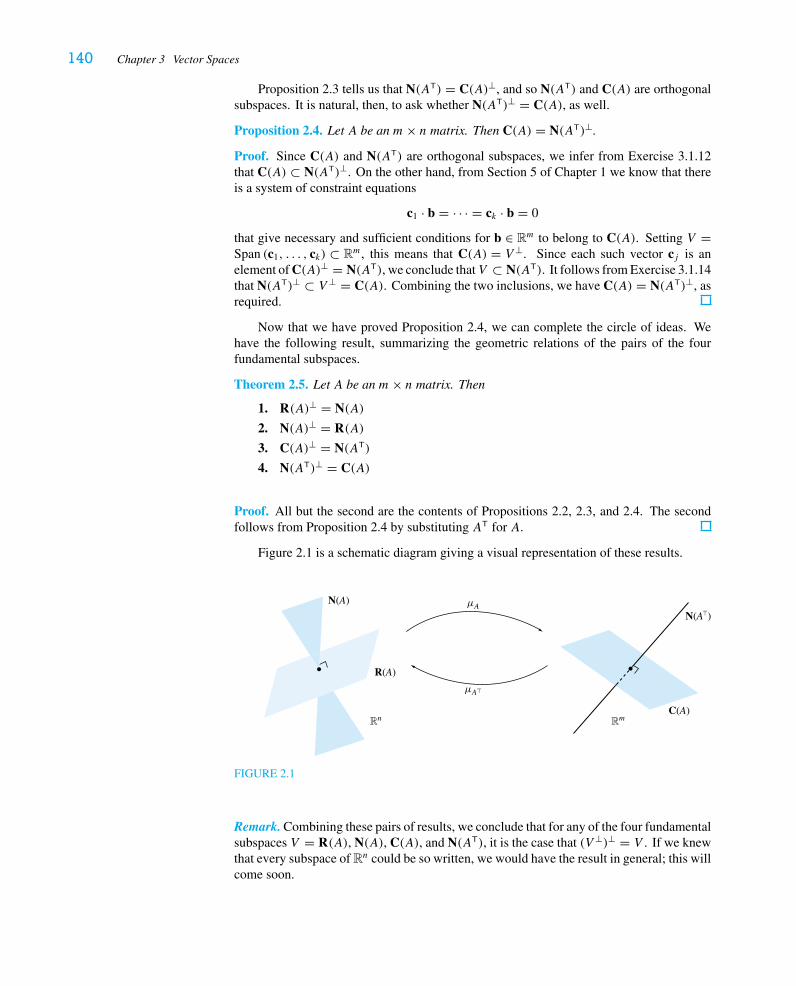
140 Chapter 3 Vector Spaces
Proposition 2.3 tells us that N(AT) = C(A)⊥, and so N(AT) and C(A) are orthogonalsubspaces. It is natural, then, to ask whether N(AT)⊥ = C(A), as well.
Proposition 2.4. Let A be an m× n matrix. Then C(A) = N(AT)⊥.
Proof. Since C(A) and N(AT) are orthogonal subspaces, we infer from Exercise 3.1.12that C(A) ⊂ N(AT)⊥. On the other hand, from Section 5 of Chapter 1 we know that thereis a system of constraint equations
c1 · b = · · · = ck · b = 0
that give necessary and sufficient conditions for b ∈ Rm to belong to C(A). Setting V =Span (c1, . . . , ck) ⊂ Rm, this means that C(A) = V ⊥. Since each such vector cj is anelement of C(A)⊥ = N(AT), we conclude thatV ⊂ N(AT). It follows from Exercise 3.1.14that N(AT)⊥ ⊂ V ⊥ = C(A). Combining the two inclusions, we have C(A) = N(AT)⊥, asrequired.
Now that we have proved Proposition 2.4, we can complete the circle of ideas. Wehave the following result, summarizing the geometric relations of the pairs of the fourfundamental subspaces.
Theorem 2.5. Let A be an m× n matrix. Then
1. R(A)⊥ = N(A)
2. N(A)⊥ = R(A)
3. C(A)⊥ = N(AT)
4. N(AT)⊥ = C(A)
Proof. All but the second are the contents of Propositions 2.2, 2.3, and 2.4. The secondfollows from Proposition 2.4 by substituting AT for A.
Figure 2.1 is a schematic diagram giving a visual representation of these results.
N(A)
R(A)
C(A)Rn Rm
μA
μA�
N(A�)
FIGURE 2.1
Remark. Combining these pairs of results, we conclude that for any of the four fundamentalsubspaces V = R(A), N(A), C(A), and N(AT), it is the case that (V ⊥)⊥ = V . If we knewthat every subspace of Rn could be so written, we would have the result in general; this willcome soon.
2 The Four Fundamental Subspaces 141
EXAMPLE 3
Let’s look for matrices whose row spaces are the plane in R3 spanned by
⎡⎢⎣
1
1
1
⎤⎥⎦ and
⎡⎢⎣
1
−1
−1
⎤⎥⎦
and satisfy the extra conditions given below. Note, first of all, that these must be m× 3matrices for some positive integers m.
(a) Suppose we want such a matrix A with
⎡⎢⎣
1
2
−1
⎤⎥⎦ in its nullspace. Remember that
N(A) = R(A)⊥. We cannot succeed: Although
⎡⎢⎣
1
2
−1
⎤⎥⎦ is orthogonal to
⎡⎢⎣
1
−1
−1
⎤⎥⎦, it is
not orthogonal to
⎡⎢⎣
1
1
1
⎤⎥⎦ and hence not orthogonal to every vector in the row space.
(b) Suppose we want such a matrix with its column space equal to R2. Now we win: Weneed a 2 × 3 matrix, and we just try
A =[
1 1 1
1 −1 −1
].
Then C(A) = Span
([1
1
],
[1
−1
])= R2, as required.
(c) Suppose we want such a matrix A whose column space is spanned by
[1
−1
]. This
seems impossible, but here’s an argument to that effect. If we had such a matrix
A, note that C(A)⊥ = N(AT) is spanned by
[1
1
], and so we would have to have
A1 + A2 = 0. This means that the row space of A is a line.
(d) Following this reasoning, let’s look for a matrix A whose column space is spanned
by
⎡⎢⎣
1
0
1
⎤⎥⎦ and
⎡⎢⎣
0
1
1
⎤⎥⎦. We note that A now must be a 3 × 3 matrix. As before, note that
⎡⎢⎣
1
1
−1
⎤⎥⎦ ∈ C(A)⊥ = N(AT), and so the third row of Amust be the sum of the first two
rows. So now we just try
A =
⎡⎢⎢⎣
1 1 1
1 −1 −1
2 0 0
⎤⎥⎥⎦ .
142 Chapter 3 Vector Spaces
Perhaps it’s not obvious thatA really works, but if we add the first and second columns,
we get
⎡⎢⎣
2
0
2
⎤⎥⎦, and if we subtract them we get
⎡⎢⎣
0
2
2
⎤⎥⎦, so C(A) contains both the desired
vectors and hence their span. We leave it to the reader to check that C(A) is not largerthan this span.
Exercises 3.2
1.�∗ Show that if B is obtained from A by performing one or more row operations, thenR(B) = R(A).
2. What vectors b are in the column space ofA in each case? (Give constraint equations.)Check that the coefficients of the constraint equations give linear combinations of therows of A summing to 0.
a.∗ A =⎡⎢⎣
3 −1
6 −2
−9 3
⎤⎥⎦ b.∗ A =
⎡⎢⎣
1 1 1
−1 1 2
1 3 −5
⎤⎥⎦ c. A =
⎡⎢⎢⎢⎣
1 −2 1
0 1 3
−1 3 0
1 0 −1
⎤⎥⎥⎥⎦
3. Given each matrix A, find matricesX and Y so that C(A) = N(X) and N(A) = C(Y ).
a.∗ A =⎡⎢⎣
3 −1
6 −2
−9 3
⎤⎥⎦ b. A =
⎡⎢⎣
1 1 0
2 1 1
1 −1 2
⎤⎥⎦ c. A =
⎡⎢⎢⎢⎣
1 1 1
1 2 0
1 1 1
1 0 2
⎤⎥⎥⎥⎦
4.∗ Let A =⎡⎢⎣
1 2 1 1
−1 0 3 4
2 2 −2 −3
⎤⎥⎦.
a. Give constraint equations for C(A).b. Find vectors spanning N(AT).
5.∗ Let
L =
⎡⎢⎢⎣
1 0 0
2 1 0
1 −1 1
⎤⎥⎥⎦ and U =
⎡⎢⎢⎣
1 2 1 1
0 0 2 −2
0 0 0 0
⎤⎥⎥⎦ .
If A = LU , give vectors that span R(A), C(A), and N(A).
6. a. Construct a matrix whose column space contains
⎡⎢⎣
1
1
1
⎤⎥⎦ and
⎡⎢⎣
0
1
1
⎤⎥⎦ and whose nullspace
contains
⎡⎢⎣
1
0
1
⎤⎥⎦ and
⎡⎢⎣
0
1
0
⎤⎥⎦, or explain why none can exist.
b.∗ Construct a matrix whose column space contains
⎡⎢⎣
1
1
1
⎤⎥⎦ and
⎡⎢⎣
0
1
1
⎤⎥⎦ and whose nullspace
contains
⎡⎢⎢⎢⎣
1
0
1
0
⎤⎥⎥⎥⎦ and
⎡⎢⎢⎢⎣
1
0
0
1
⎤⎥⎥⎥⎦, or explain why none can exist.
3 Linear Independence and Basis 143
7. Let A =⎡⎢⎣
1 1 0
1 1 0
0 1 1
⎤⎥⎦ and B =
⎡⎢⎣
1 1 0
−1 −1 0
0 −1 −1
⎤⎥⎦.
a. Give C(A) and C(B). Are they lines, planes, or all of R3?
b. Describe C(A+ B) and C(A)+ C(B). Compare your answers.
8. a.∗ Construct a 3 × 3 matrix A with C(A) ⊂ N(A).b. Construct a 3 × 3 matrix A with N(A) ⊂ C(A).c. Do you think there can be a 3 × 3 matrix A with N(A) = C(A)? Why or why not?
d. Construct a 4 × 4 matrix A with C(A) = N(A).
9.∗ Let A be an m× n matrix and recall that we have the associated function μA : Rn →Rm defined by μA(x) = Ax. Show that μA is a one-to-one function if and only ifN(A) = {0}.
10.� Let A be an m× n matrix and B be an n× p matrix. Prove thata. N(B) ⊂ N(AB).b. C(AB) ⊂ C(A). (Hint: Use Proposition 2.1.)
c. N(B) = N(AB) when A is n× n and nonsingular. (Hint: See the box on p. 12.)
d. C(AB) = C(A) when B is n× n and nonsingular.
11.� Let A be an m× n matrix. Prove that N(ATA) = N(A). (Hint: Use Exercise 10 andExercise 2.5.15.)
12. Suppose A and B are m× n matrices. Prove that C(A) and C(B) are orthogonalsubspaces of Rm if and only if ATB = O.
13. Suppose A is an n× n matrix with the property that A2 = A.a. Prove that C(A) = {x ∈ Rn : x = Ax}.b. Prove that N(A) = {x ∈ Rn : x = u − Au for some u ∈ Rn}.c. Prove that C(A) ∩ N(A) = {0}.d. Prove that C(A)+ N(A) = Rn.
3 Linear Independence and Basis
In view of our discussion in the preceding section, it is natural to ask the following question:
Given vectors v1, . . . , vk ∈ Rn and v ∈ Rn, is v ∈ Span (v1, . . . , vk)?
Of course, we recognize that this is a question of whether there exist scalars c1, . . . , ck suchthat v = c1v1 + c2v2 + · · · + ckvk . As we are well aware, this is, in turn, a question ofwhether a certain (inhomogeneous) system of linear equations has a solution. As we sawin Chapter 1, one is often interested in the allied question: Is that solution unique?
EXAMPLE 1
Let
v1 =
⎡⎢⎢⎣
1
1
2
⎤⎥⎥⎦ , v2 =
⎡⎢⎢⎣
1
−1
0
⎤⎥⎥⎦ , v3 =
⎡⎢⎢⎣
1
0
1
⎤⎥⎥⎦ , and v =
⎡⎢⎢⎣
1
1
0
⎤⎥⎥⎦ .
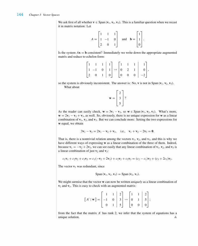
144 Chapter 3 Vector Spaces
We ask first of all whether v ∈ Span (v1, v2, v3). This is a familiar question when we recastit in matrix notation: Let
A =
⎡⎢⎢⎣
1 1 1
1 −1 0
2 0 1
⎤⎥⎥⎦ and b =
⎡⎢⎢⎣
1
1
0
⎤⎥⎥⎦ .
Is the system Ax = b consistent? Immediately we write down the appropriate augmentedmatrix and reduce to echelon form:
⎡⎢⎢⎣
1 1 1 1
1 −1 0 1
2 0 1 0
⎤⎥⎥⎦ �
⎡⎢⎢⎣
1 1 1 1
0 2 1 0
0 0 0 −2
⎤⎥⎥⎦ ,
so the system is obviously inconsistent. The answer is: No, v is not in Span (v1, v2, v3).What about
w =
⎡⎢⎢⎣
2
3
5
⎤⎥⎥⎦ ?
As the reader can easily check, w = 3v1 − v3, so w ∈ Span (v1, v2, v3). What’s more,w = 2v1 − v2 + v3, as well. So, obviously, there is no unique expression for w as a linearcombination of v1, v2, and v3. But we can conclude more: Setting the two expressions forw equal, we obtain
3v1 − v3 = 2v1 − v2 + v3, i.e., v1 + v2 − 2v3 = 0.
That is, there is a nontrivial relation among the vectors v1, v2, and v3, and this is why wehave different ways of expressing w as a linear combination of the three of them. Indeed,because v1 = −v2 + 2v3, we can see easily that any linear combination of v1, v2, and v3 isa linear combination of just v2 and v3:
c1v1 + c2v2 + c3v3 = c1(−v2 + 2v3)+ c2v2 + c3v3 = (c2 − c1)v2 + (c3 + 2c1)v3.
The vector v1 was redundant, since
Span (v1, v2, v3) = Span (v2, v3).
We might surmise that the vector w can now be written uniquely as a linear combination ofv2 and v3. This is easy to check with an augmented matrix:
[A′ | w
] =
⎡⎢⎢⎣
1 1 2
−1 0 3
0 1 5
⎤⎥⎥⎦ �
⎡⎢⎢⎣
1 1 2
0 1 5
0 0 0
⎤⎥⎥⎦ ;
from the fact that the matrix A′ has rank 2, we infer that the system of equations has aunique solution.
3 Linear Independence and Basis 145
In the language of functions, the question of uniqueness is the question of whetherthe function μA : R3 → R3 is one-to-one. Remember that we say f is a one-to-onefunction if
whenever a �= b, it must be the case that f (a) �= f (b).
Given some function y = f (x), we might ask if, for a certain value r , we can solvethe equation f (x) = r . When r is in the image of the function, there is at least onesolution. Is the solution unique? If f is a one-to-one function, there can be at mostone solution of the equation f (x) = r .
Next we show that the question of uniqueness we raised earlier can be reduced to onebasic question, which will be crucial to all our future work.
Proposition 3.1. Let v1, . . . , vk ∈ Rn. If the zero vector has a unique expression as a linearcombination of v1, . . . , vk , that is, if
c1v1 + c2v2 + · · · + ckvk = 0 ⇒ c1 = c2 = · · · = ck = 0,
then every vector v ∈ Span (v1, . . . , vk) has a unique expression as a linear combinationof v1, . . . , vk .
Proof. By considering the matrix A whose column vectors are v1, . . . , vk , we can de-duce this immediately from Proposition 5.4 of Chapter 1. However, we prefer to give acoordinate-free proof that is typical of many of the arguments we shall be encountering fora while.
Suppose that for some v ∈ Span (v1, . . . , vk) there are two expressions
v = c1v1 + c2v2 + · · · + ckvk and
v = d1v1 + d2v2 + · · · + dkvk.Then, subtracting, we obtain
0 = (c1 − d1)v1 + · · · + (ck − dk)vk.Since the only way to express the zero vector as a linear combination of v1, . . . , vk iswith every coefficient equal to 0, we conclude that c1 − d1 = c2 − d2 = · · · = ck − dk =0, which means, of course, that c1 = d1, c2 = d2, . . . , ck = dk . That is, v has a uniqueexpression as a linear combination of v1, . . . , vk .
This discussion leads us to make the following definition.
Definition. The (indexed) set of vectors {v1, . . . , vk} is called linearly independent if
c1v1 + c2v2 + · · · + ckvk = 0 ⇒ c1 = c2 = · · · = ck = 0,
that is, if the only way of expressing the zero vector as a linear combination of v1, . . . , vkis the trivial linear combination 0v1 + · · · + 0vk .
The set of vectors {v1, . . . , vk} is called linearly dependent if it is not linearlyindependent—i.e., if there is some expression
c1v1 + c2v2 + · · · + ckvk = 0, where not all the ci’s are 0.
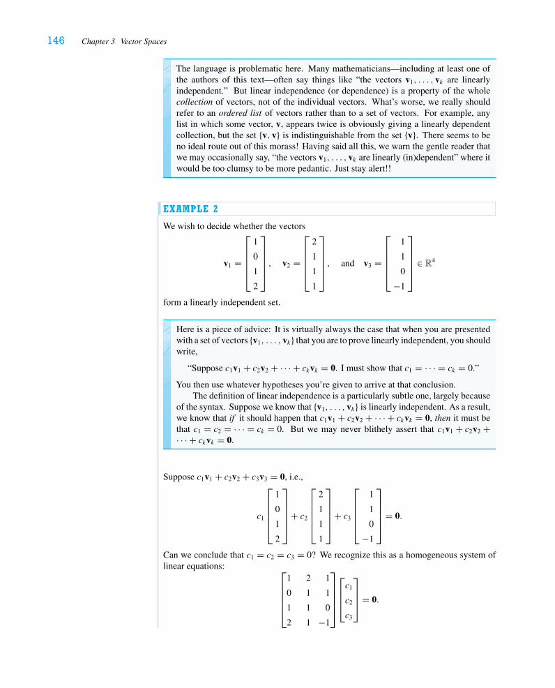
146 Chapter 3 Vector Spaces
The language is problematic here. Many mathematicians—including at least one ofthe authors of this text—often say things like “the vectors v1, . . . , vk are linearlyindependent.” But linear independence (or dependence) is a property of the wholecollection of vectors, not of the individual vectors. What’s worse, we really shouldrefer to an ordered list of vectors rather than to a set of vectors. For example, anylist in which some vector, v, appears twice is obviously giving a linearly dependentcollection, but the set {v, v} is indistinguishable from the set {v}. There seems to beno ideal route out of this morass! Having said all this, we warn the gentle reader thatwe may occasionally say, “the vectors v1, . . . , vk are linearly (in)dependent” where itwould be too clumsy to be more pedantic. Just stay alert!!
EXAMPLE 2
We wish to decide whether the vectors
v1 =
⎡⎢⎢⎢⎢⎣
1
0
1
2
⎤⎥⎥⎥⎥⎦, v2 =
⎡⎢⎢⎢⎢⎣
2
1
1
1
⎤⎥⎥⎥⎥⎦, and v3 =
⎡⎢⎢⎢⎢⎣
1
1
0
−1
⎤⎥⎥⎥⎥⎦
∈ R4
form a linearly independent set.
Here is a piece of advice: It is virtually always the case that when you are presentedwith a set of vectors {v1, . . . , vk} that you are to prove linearly independent, you shouldwrite,
“Suppose c1v1 + c2v2 + · · · + ckvk = 0. I must show that c1 = · · · = ck = 0.”
You then use whatever hypotheses you’re given to arrive at that conclusion.The definition of linear independence is a particularly subtle one, largely because
of the syntax. Suppose we know that {v1, . . . , vk} is linearly independent. As a result,we know that if it should happen that c1v1 + c2v2 + · · · + ckvk = 0, then it must bethat c1 = c2 = · · · = ck = 0. But we may never blithely assert that c1v1 + c2v2 +· · · + ckvk = 0.
Suppose c1v1 + c2v2 + c3v3 = 0, i.e.,
c1
⎡⎢⎢⎢⎢⎣
1
0
1
2
⎤⎥⎥⎥⎥⎦
+ c2
⎡⎢⎢⎢⎢⎣
2
1
1
1
⎤⎥⎥⎥⎥⎦
+ c3
⎡⎢⎢⎢⎢⎣
1
1
0
−1
⎤⎥⎥⎥⎥⎦
= 0.
Can we conclude that c1 = c2 = c3 = 0? We recognize this as a homogeneous system oflinear equations: ⎡
⎢⎢⎢⎢⎣
1 2 1
0 1 1
1 1 0
2 1 −1
⎤⎥⎥⎥⎥⎦
⎡⎢⎢⎣c1
c2
c3
⎤⎥⎥⎦ = 0.
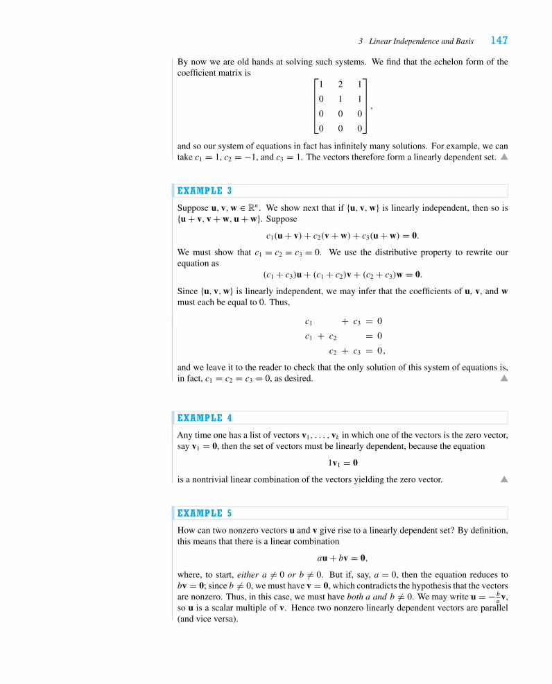
3 Linear Independence and Basis 147
By now we are old hands at solving such systems. We find that the echelon form of thecoefficient matrix is ⎡
⎢⎢⎢⎢⎣
1 2 1
0 1 1
0 0 0
0 0 0
⎤⎥⎥⎥⎥⎦,
and so our system of equations in fact has infinitely many solutions. For example, we cantake c1 = 1, c2 = −1, and c3 = 1. The vectors therefore form a linearly dependent set.
EXAMPLE 3
Suppose u, v,w ∈ Rn. We show next that if {u, v,w} is linearly independent, then so is{u + v, v + w, u + w}. Suppose
c1(u + v)+ c2(v + w)+ c3(u + w) = 0.
We must show that c1 = c2 = c3 = 0. We use the distributive property to rewrite ourequation as
(c1 + c3)u + (c1 + c2)v + (c2 + c3)w = 0.
Since {u, v,w} is linearly independent, we may infer that the coefficients of u, v, and wmust each be equal to 0. Thus,
c1 + c3 = 0
c1 + c2 = 0
c2 + c3 = 0 ,
and we leave it to the reader to check that the only solution of this system of equations is,in fact, c1 = c2 = c3 = 0, as desired.
EXAMPLE 4
Any time one has a list of vectors v1, . . . , vk in which one of the vectors is the zero vector,say v1 = 0, then the set of vectors must be linearly dependent, because the equation
1v1 = 0
is a nontrivial linear combination of the vectors yielding the zero vector.
EXAMPLE 5
How can two nonzero vectors u and v give rise to a linearly dependent set? By definition,this means that there is a linear combination
au + bv = 0,
where, to start, either a �= 0 or b �= 0. But if, say, a = 0, then the equation reduces tobv = 0; since b �= 0, we must have v = 0, which contradicts the hypothesis that the vectorsare nonzero. Thus, in this case, we must have both a and b �= 0. We may write u = − b
av,
so u is a scalar multiple of v. Hence two nonzero linearly dependent vectors are parallel(and vice versa).
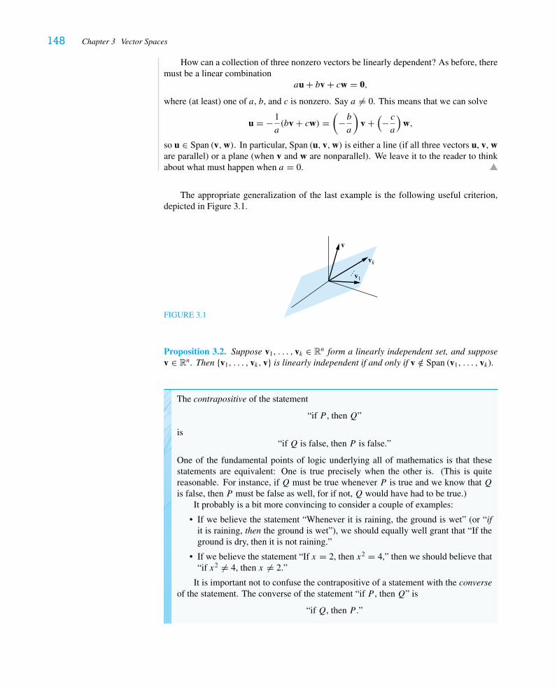
148 Chapter 3 Vector Spaces
How can a collection of three nonzero vectors be linearly dependent? As before, theremust be a linear combination
au + bv + cw = 0,
where (at least) one of a, b, and c is nonzero. Say a �= 0. This means that we can solve
u = −1
a(bv + cw) =
(−ba
)v +
(− ca
)w,
so u ∈ Span (v,w). In particular, Span (u, v,w) is either a line (if all three vectors u, v, ware parallel) or a plane (when v and w are nonparallel). We leave it to the reader to thinkabout what must happen when a = 0.
The appropriate generalization of the last example is the following useful criterion,depicted in Figure 3.1.
FIGURE 3.1
v
v1
vk
…Proposition 3.2. Suppose v1, . . . , vk ∈ Rn form a linearly independent set, and supposev ∈ Rn. Then {v1, . . . , vk, v} is linearly independent if and only if v /∈ Span (v1, . . . , vk).
The contrapositive of the statement
“if P , thenQ”
is“ifQ is false, then P is false.”
One of the fundamental points of logic underlying all of mathematics is that thesestatements are equivalent: One is true precisely when the other is. (This is quitereasonable. For instance, if Q must be true whenever P is true and we know that Qis false, then P must be false as well, for if not,Q would have had to be true.)
It probably is a bit more convincing to consider a couple of examples:
• If we believe the statement “Whenever it is raining, the ground is wet” (or “ifit is raining, then the ground is wet”), we should equally well grant that “If theground is dry, then it is not raining.”
• If we believe the statement “If x = 2, then x2 = 4,” then we should believe that“if x2 �= 4, then x �= 2.”
It is important not to confuse the contrapositive of a statement with the converseof the statement. The converse of the statement “if P , thenQ” is
“ifQ, then P .”
3 Linear Independence and Basis 149
Note that even if we believe our two earlier statements, we do not believe their con-verses:
• “If the ground is wet, then it is raining”—it may have stopped raining a whileago, or someone may have washed a car earlier.
• “If x2 = 4, then x = 2”—even though this is a common error, it is an errornevertheless: x might be −2.
Proof. We will prove the contrapositive: Still supposing that v1, . . . , vk ∈ Rn form alinearly independent set,
{v1, . . . , vk, v} is linearly dependent if and only if v ∈ Span (v1, . . . , vk).
Suppose that v ∈ Span (v1, . . . , vk). Then v = c1v1 + c2v2 + · · · + ckvk for some scalarsc1, . . . , ck , so
c1v1 + c2v2 + · · · + ckvk + (−1)v = 0,
from which we conclude that {v1, . . . , vk, v} is linearly dependent (since at least one of thecoefficients is nonzero).
Now suppose {v1, . . . , vk, v} is linearly dependent. This means that there are scalarsc1, . . . , ck , and c, not all 0, such that
c1v1 + c2v2 + · · · + ckvk + cv = 0.
Note that we cannot have c = 0: For if c were 0, we’d have c1v1 + c2v2 + · · · + ckvk = 0,and linear independence of {v1, . . . , vk} implies c1 = · · · = ck = 0, which contradicts ourassumption that {v1, . . . , vk, v} is linearly dependent. Therefore c �= 0, and so
v = −1
c(c1v1 + c2v2 + · · · + ckvk) =
(−c1
c
)v1 +
(−c2
c
)v2 + · · · +
(−ckc
)vk,
which tells us that v ∈ Span (v1, . . . , vk), as required.
We now understand that when we have a set of linearly independent vectors, no propersubset will yield the same span. In other words, we will have an “efficient” set of spanningvectors (that is, there is no redundancy in the vectors we’ve chosen; no proper subset willdo). This motivates the following definition.
Definition. Let V ⊂ Rn be a subspace. The set of vectors {v1, . . . , vk} is called a basisfor V if
(i) v1, . . . , vk span V , that is, V = Span (v1, . . . , vk), and
(ii) {v1, . . . , vk} is linearly independent.
We comment that the plural of basis is bases.4
EXAMPLE 6
Let e1 = (1, 0, . . . , 0), e2 = (0, 1, 0, . . . , 0), . . . , en = (0, . . . , 0, 1) ∈ Rn. Then {e1, . . . , en}is a basis for Rn, called the standard basis. To check this, we must establish that properties(i) and (ii) above hold for V = Rn. The first is obvious: If x = (x1, . . . , xn) ∈ Rn, then x =
4Pronounced basez, to rhyme with Macy’s.
150 Chapter 3 Vector Spaces
x1e1 + x2e2 + · · · + xnen. The second is not much harder. Suppose c1e1 + c2e2 + · · · +cnen = 0. This means that (c1, c2, . . . , cn) = (0, 0, . . . , 0), and so c1 = c2 = · · · = cn = 0.
EXAMPLE 7
Consider the plane given by V = {x ∈ R3 : x1 − x2 + 2x3 = 0} ⊂ R3. Our algorithms ofChapter 1 tell us that the vectors
v1 =
⎡⎢⎢⎣
1
1
0
⎤⎥⎥⎦ and v2 =
⎡⎢⎢⎣
−2
0
1
⎤⎥⎥⎦
span V . Since these vectors are not parallel, it follows from Example 5 that they must belinearly independent.
For the practice, however, we give a direct argument. Suppose
c1v1 + c2v2 = c1
⎡⎢⎢⎣
1
1
0
⎤⎥⎥⎦+ c2
⎡⎢⎢⎣
−2
0
1
⎤⎥⎥⎦ = 0.
Writing out the entries explicitly, we obtain⎡⎢⎢⎣c1 − 2c2
c1
c2
⎤⎥⎥⎦ =
⎡⎢⎢⎣
0
0
0
⎤⎥⎥⎦ ,
from which we conclude that c1 = c2 = 0, as required. (For future reference, we notethat this information came from the free variable “slots.”) Therefore, {v1, v2} is linearlyindependent and gives a basis for V , as required.
The following observation may prove useful.
Corollary 3.3. Let V ⊂ Rn be a subspace, and let v1, . . . , vk ∈ V . Then {v1, . . . , vk} is abasis for V if and only if every vector of V can be written uniquely as a linear combinationof v1, . . . , vk .
Proof. This is immediate from Proposition 3.1.
This result is so important that we introduce a bit of terminology.
Definition. When we write v = c1v1 + c2v2 + · · · + ckvk , we refer to c1, . . . , ck as thecoordinates of v with respect to the (ordered) basis {v1, . . . , vk}.
EXAMPLE 8
Consider the three vectors
v1 =
⎡⎢⎢⎣
1
2
1
⎤⎥⎥⎦ , v2 =
⎡⎢⎢⎣
1
1
2
⎤⎥⎥⎦ , and v3 =
⎡⎢⎢⎣
1
0
2
⎤⎥⎥⎦ .
3 Linear Independence and Basis 151
Let’s take a general vector b ∈ R3 and ask first of all whether it has a unique expression asa linear combination of v1, v2, and v3. Forming the augmented matrix and row reducing,we find ⎡
⎢⎢⎣1 1 1 b1
2 1 0 b2
1 2 2 b3
⎤⎥⎥⎦ �
⎡⎢⎢⎣
1 0 0 2b1 − b3
0 1 0 −4b1 + b2 + 2b3
0 0 1 3b1 − b2 − b3
⎤⎥⎥⎦ .
It follows from Corollary 3.3 that {v1, v2, v3} is a basis for R3, because an arbitrary vectorb ∈ R3 can be written in the form
b = (2b1 − b3)︸ ︷︷ ︸c1
v1 + (−4b1 + b2 + 2b3)︸ ︷︷ ︸c2
v2 + (3b1 − b2 − b3)︸ ︷︷ ︸c3
v3.
And, what’s more,
c1 = 2b1 − b3,
c2 = −4b1 + b2 + 2b3, and
c3 = 3b1 − b2 − b3
give the coordinates of b with respect to the basis {v1, v2, v3}.
Our experience in Example 8 leads us to make the following general observation:
Proposition 3.4. LetA be an n× n matrix. ThenA is nonsingular if and only if its columnvectors form a basis for Rn.
Proof. As usual, let’s denote the column vectors of A by a1, a2, . . . , an. Using Corollary3.3, we are to prove that A is nonsingular if and only if every vector in Rn can be writtenuniquely as a linear combination of a1, a2, . . . , an. But this is exactly what Proposition 5.5of Chapter 1 tells us.
Somewhat more generally (see Exercise 12), we have the following result.
EXAMPLE 9
Suppose A is a nonsingular n× n matrix and {v1, . . . , vn} is a basis for Rn. Then we wishto show that {Av1, . . . , Avn} is likewise a basis for Rn.
First, we show that {Av1, . . . , Avn} is linearly independent. Following our ritual, westart by supposing that
c1(Av1)+ c2(Av2)+ · · · + cn(Avn) = 0,
and we wish to show that c1 = · · · = cn = 0. By linearity properties we have
0 = c1Av1 + c2Av2 + · · · + cnAvn = A(c1v1)+ A(c2v2)+ · · · + A(cnvn)= A(c1v1 + c2v2 + · · · + cnvn).
Since A is nonsingular, the only solution of Ax = 0 is x = 0, and so we must have c1v1 +c2v2 + · · · + cnvn = 0. From the linear independence of {v1, . . . , vn} we now concludethat c1 = c2 = · · · = cn = 0, as required.
Now, why do these vectors span Rn? (The result follows from Exercise 1.5.13, butwe give the argument here.) Given b ∈ Rn, we know from Proposition 5.5 of Chapter 1that there is a unique x ∈ Rn with Ax = b. Since v1, . . . , vn form a basis for Rn, we can
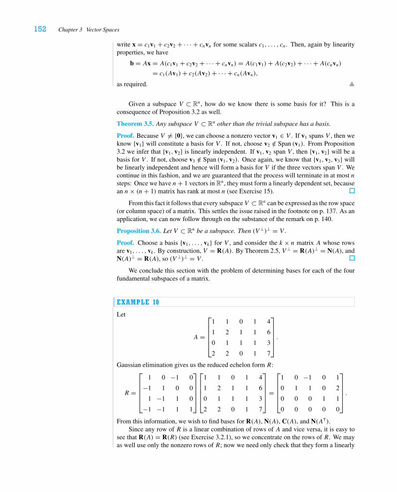
152 Chapter 3 Vector Spaces
write x = c1v1 + c2v2 + · · · + cnvn for some scalars c1, . . . , cn. Then, again by linearityproperties, we have
b = Ax = A(c1v1 + c2v2 + · · · + cnvn) = A(c1v1)+ A(c2v2)+ · · · + A(cnvn)= c1(Av1)+ c2(Av2)+ · · · + cn(Avn),
as required.
Given a subspace V ⊂ Rn, how do we know there is some basis for it? This is aconsequence of Proposition 3.2 as well.
Theorem 3.5. Any subspace V ⊂ Rn other than the trivial subspace has a basis.
Proof. Because V �= {0}, we can choose a nonzero vector v1 ∈ V . If v1 spans V , then weknow {v1} will constitute a basis for V . If not, choose v2 /∈ Span (v1). From Proposition3.2 we infer that {v1, v2} is linearly independent. If v1, v2 span V , then {v1, v2} will be abasis for V . If not, choose v3 /∈ Span (v1, v2). Once again, we know that {v1, v2, v3} willbe linearly independent and hence will form a basis for V if the three vectors span V . Wecontinue in this fashion, and we are guaranteed that the process will terminate in at most nsteps: Once we have n+ 1 vectors in Rn, they must form a linearly dependent set, becausean n× (n+ 1) matrix has rank at most n (see Exercise 15).
From this fact it follows that every subspace V ⊂ Rn can be expressed as the row space(or column space) of a matrix. This settles the issue raised in the footnote on p. 137. As anapplication, we can now follow through on the substance of the remark on p. 140.
Proposition 3.6. Let V ⊂ Rn be a subspace. Then (V ⊥)⊥ = V .
Proof. Choose a basis {v1, . . . , vk} for V , and consider the k × n matrix A whose rowsare v1, . . . , vk . By construction, V = R(A). By Theorem 2.5, V ⊥ = R(A)⊥ = N(A), andN(A)⊥ = R(A), so (V ⊥)⊥ = V .
We conclude this section with the problem of determining bases for each of the fourfundamental subspaces of a matrix.
EXAMPLE 10
Let
A =
⎡⎢⎢⎢⎢⎣
1 1 0 1 4
1 2 1 1 6
0 1 1 1 3
2 2 0 1 7
⎤⎥⎥⎥⎥⎦.
Gaussian elimination gives us the reduced echelon form R:
R =
⎡⎢⎢⎢⎢⎣
1 0 −1 0
−1 1 0 0
1 −1 1 0
−1 −1 1 1
⎤⎥⎥⎥⎥⎦
⎡⎢⎢⎢⎢⎣
1 1 0 1 4
1 2 1 1 6
0 1 1 1 3
2 2 0 1 7
⎤⎥⎥⎥⎥⎦
=
⎡⎢⎢⎢⎢⎣
1 0 −1 0 1
0 1 1 0 2
0 0 0 1 1
0 0 0 0 0
⎤⎥⎥⎥⎥⎦.
From this information, we wish to find bases for R(A), N(A), C(A), and N(AT).Since any row of R is a linear combination of rows of A and vice versa, it is easy to
see that R(A) = R(R) (see Exercise 3.2.1), so we concentrate on the rows of R. We mayas well use only the nonzero rows of R; now we need only check that they form a linearly
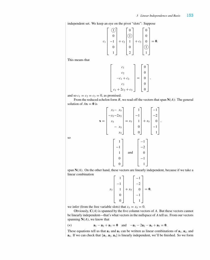
3 Linear Independence and Basis 153
independent set. We keep an eye on the pivot “slots”: Suppose
c1
⎡⎢⎢⎢⎢⎢⎢⎢⎣
�10
−1
0
1
⎤⎥⎥⎥⎥⎥⎥⎥⎦
+ c2
⎡⎢⎢⎢⎢⎢⎢⎢⎣
0�1
1
0
2
⎤⎥⎥⎥⎥⎥⎥⎥⎦
+ c3
⎡⎢⎢⎢⎢⎢⎢⎢⎣
0
0
0�1
1
⎤⎥⎥⎥⎥⎥⎥⎥⎦
= 0.
This means that⎡⎢⎢⎢⎢⎢⎢⎢⎣
c1
c2
−c1 + c2
c3
c1 + 2c2 + c3
⎤⎥⎥⎥⎥⎥⎥⎥⎦
=
⎡⎢⎢⎢⎢⎢⎢⎢⎣
0
0
0
0
0
⎤⎥⎥⎥⎥⎥⎥⎥⎦,
and so c1 = c2 = c3 = 0, as promised.From the reduced echelon formR, we read off the vectors that span N(A): The general
solution of Ax = 0 is
x =
⎡⎢⎢⎢⎢⎢⎢⎢⎣
x3− x5
−x3−2x5
x3
− x5
x5
⎤⎥⎥⎥⎥⎥⎥⎥⎦
= x3
⎡⎢⎢⎢⎢⎢⎢⎢⎣
1
−1
1
0
0
⎤⎥⎥⎥⎥⎥⎥⎥⎦
+ x5
⎡⎢⎢⎢⎢⎢⎢⎢⎣
−1
−2
0
−1
1
⎤⎥⎥⎥⎥⎥⎥⎥⎦,
so ⎡⎢⎢⎢⎢⎢⎢⎢⎣
1
−1
1
0
0
⎤⎥⎥⎥⎥⎥⎥⎥⎦
and
⎡⎢⎢⎢⎢⎢⎢⎢⎣
−1
−2
0
−1
1
⎤⎥⎥⎥⎥⎥⎥⎥⎦
span N(A). On the other hand, these vectors are linearly independent, because if we take alinear combination
x3
⎡⎢⎢⎢⎢⎢⎢⎢⎣
1
−1
1
0
0
⎤⎥⎥⎥⎥⎥⎥⎥⎦
+ x5
⎡⎢⎢⎢⎢⎢⎢⎢⎣
−1
−2
0
−1
1
⎤⎥⎥⎥⎥⎥⎥⎥⎦
= 0,
we infer (from the free variable slots) that x3 = x5 = 0.Obviously, C(A) is spanned by the five column vectors of A. But these vectors cannot
be linearly independent—that’s what vectors in the nullspace ofA tell us. From our vectorsspanning N(A), we know that
(∗) a1 − a2 + a3 = 0 and −a1 − 2a2 − a4 + a5 = 0.
These equations tell us that a3 and a5 can be written as linear combinations of a1, a2, anda4. If we can check that {a1, a2, a4} is linearly independent, we’ll be finished. So we form
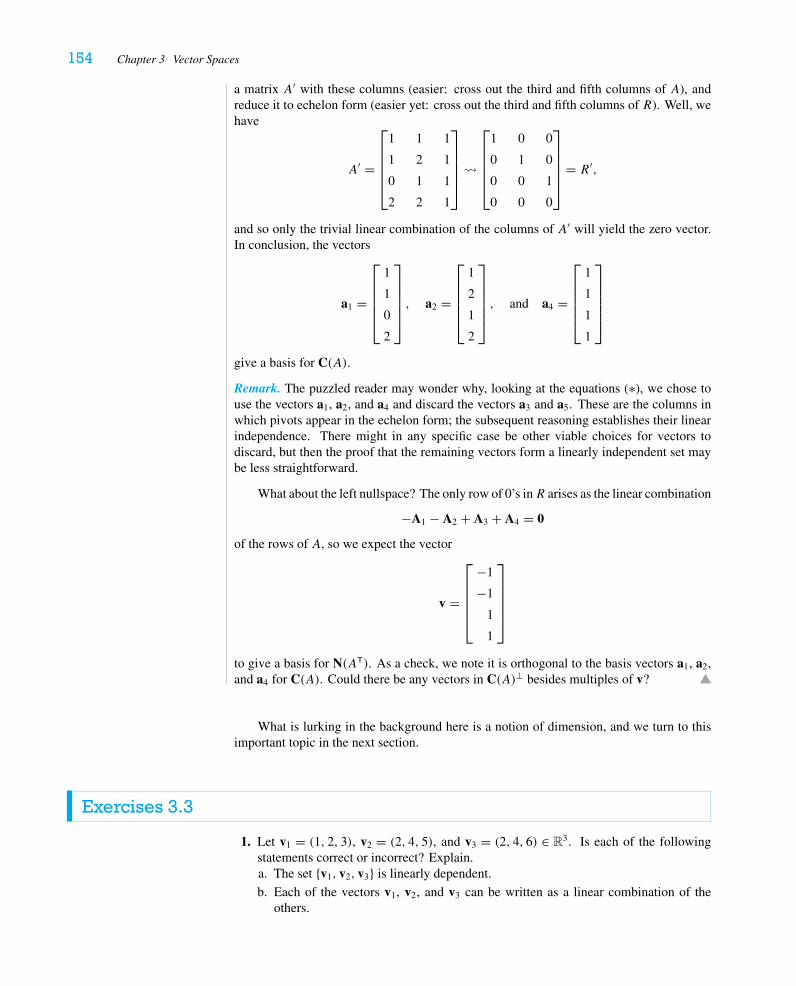
154 Chapter 3 Vector Spaces
a matrix A′ with these columns (easier: cross out the third and fifth columns of A), andreduce it to echelon form (easier yet: cross out the third and fifth columns of R). Well, wehave
A′ =
⎡⎢⎢⎢⎢⎣
1 1 1
1 2 1
0 1 1
2 2 1
⎤⎥⎥⎥⎥⎦
�
⎡⎢⎢⎢⎢⎣
1 0 0
0 1 0
0 0 1
0 0 0
⎤⎥⎥⎥⎥⎦
= R′,
and so only the trivial linear combination of the columns of A′ will yield the zero vector.In conclusion, the vectors
a1 =
⎡⎢⎢⎢⎢⎣
1
1
0
2
⎤⎥⎥⎥⎥⎦, a2 =
⎡⎢⎢⎢⎢⎣
1
2
1
2
⎤⎥⎥⎥⎥⎦, and a4 =
⎡⎢⎢⎢⎢⎣
1
1
1
1
⎤⎥⎥⎥⎥⎦
give a basis for C(A).
Remark. The puzzled reader may wonder why, looking at the equations (∗), we chose touse the vectors a1, a2, and a4 and discard the vectors a3 and a5. These are the columns inwhich pivots appear in the echelon form; the subsequent reasoning establishes their linearindependence. There might in any specific case be other viable choices for vectors todiscard, but then the proof that the remaining vectors form a linearly independent set maybe less straightforward.
What about the left nullspace? The only row of 0’s inR arises as the linear combination
−A1 − A2 + A3 + A4 = 0
of the rows of A, so we expect the vector
v =
⎡⎢⎢⎢⎢⎣
−1
−1
1
1
⎤⎥⎥⎥⎥⎦
to give a basis for N(AT). As a check, we note it is orthogonal to the basis vectors a1, a2,and a4 for C(A). Could there be any vectors in C(A)⊥ besides multiples of v?
What is lurking in the background here is a notion of dimension, and we turn to thisimportant topic in the next section.
Exercises 3.3
1. Let v1 = (1, 2, 3), v2 = (2, 4, 5), and v3 = (2, 4, 6) ∈ R3. Is each of the followingstatements correct or incorrect? Explain.a. The set {v1, v2, v3} is linearly dependent.
b. Each of the vectors v1, v2, and v3 can be written as a linear combination of theothers.
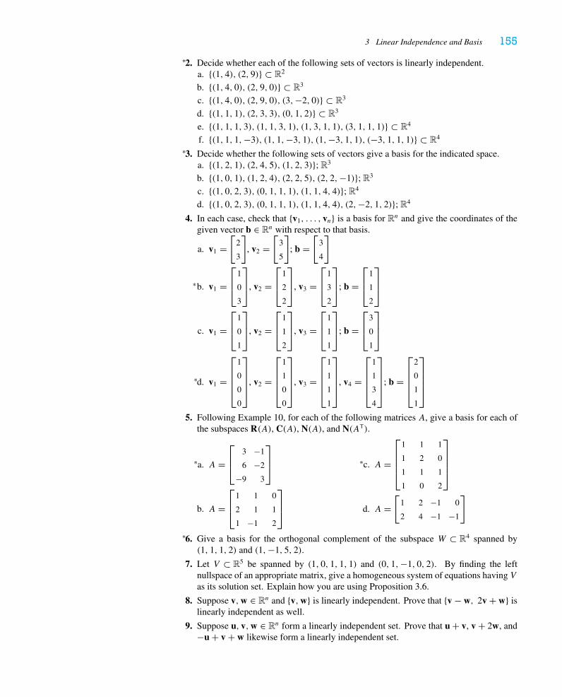
3 Linear Independence and Basis 155
2.∗ Decide whether each of the following sets of vectors is linearly independent.a. {(1, 4), (2, 9)} ⊂ R2
b. {(1, 4, 0), (2, 9, 0)} ⊂ R3
c. {(1, 4, 0), (2, 9, 0), (3,−2, 0)} ⊂ R3
d. {(1, 1, 1), (2, 3, 3), (0, 1, 2)} ⊂ R3
e. {(1, 1, 1, 3), (1, 1, 3, 1), (1, 3, 1, 1), (3, 1, 1, 1)} ⊂ R4
f. {(1, 1, 1,−3), (1, 1,−3, 1), (1,−3, 1, 1), (−3, 1, 1, 1)} ⊂ R4
3.∗ Decide whether the following sets of vectors give a basis for the indicated space.a. {(1, 2, 1), (2, 4, 5), (1, 2, 3)}; R3
b. {(1, 0, 1), (1, 2, 4), (2, 2, 5), (2, 2,−1)}; R3
c. {(1, 0, 2, 3), (0, 1, 1, 1), (1, 1, 4, 4)}; R4
d. {(1, 0, 2, 3), (0, 1, 1, 1), (1, 1, 4, 4), (2,−2, 1, 2)}; R4
4. In each case, check that {v1, . . . , vn} is a basis for Rn and give the coordinates of thegiven vector b ∈ Rn with respect to that basis.
a. v1 =[
2
3
], v2 =
[3
5
]; b =
[3
4
]
b.∗ v1 =⎡⎢⎣
1
0
3
⎤⎥⎦, v2 =
⎡⎢⎣
1
2
2
⎤⎥⎦, v3 =
⎡⎢⎣
1
3
2
⎤⎥⎦; b =
⎡⎢⎣
1
1
2
⎤⎥⎦
c. v1 =⎡⎢⎣
1
0
1
⎤⎥⎦, v2 =
⎡⎢⎣
1
1
2
⎤⎥⎦, v3 =
⎡⎢⎣
1
1
1
⎤⎥⎦; b =
⎡⎢⎣
3
0
1
⎤⎥⎦
d.∗ v1 =
⎡⎢⎢⎢⎣
1
0
0
0
⎤⎥⎥⎥⎦, v2 =
⎡⎢⎢⎢⎣
1
1
0
0
⎤⎥⎥⎥⎦, v3 =
⎡⎢⎢⎢⎣
1
1
1
1
⎤⎥⎥⎥⎦, v4 =
⎡⎢⎢⎢⎣
1
1
3
4
⎤⎥⎥⎥⎦; b =
⎡⎢⎢⎢⎣
2
0
1
1
⎤⎥⎥⎥⎦
5. Following Example 10, for each of the following matrices A, give a basis for each ofthe subspaces R(A), C(A), N(A), and N(AT).
a.∗ A =⎡⎢⎣
3 −1
6 −2
−9 3
⎤⎥⎦
b. A =⎡⎢⎣
1 1 0
2 1 1
1 −1 2
⎤⎥⎦
c.∗ A =
⎡⎢⎢⎢⎣
1 1 1
1 2 0
1 1 1
1 0 2
⎤⎥⎥⎥⎦
d. A =[
1 2 −1 0
2 4 −1 −1
]
6.∗ Give a basis for the orthogonal complement of the subspace W ⊂ R4 spanned by(1, 1, 1, 2) and (1,−1, 5, 2).
7. Let V ⊂ R5 be spanned by (1, 0, 1, 1, 1) and (0, 1,−1, 0, 2). By finding the leftnullspace of an appropriate matrix, give a homogeneous system of equations having Vas its solution set. Explain how you are using Proposition 3.6.
8. Suppose v,w ∈ Rn and {v,w} is linearly independent. Prove that {v − w, 2v + w} islinearly independent as well.
9. Suppose u, v,w ∈ Rn form a linearly independent set. Prove that u + v, v + 2w, and−u + v + w likewise form a linearly independent set.
156 Chapter 3 Vector Spaces
10.� Suppose v1, . . . , vk are nonzero vectors with the property that vi · vj = 0 wheneveri �= j . Prove that {v1, . . . , vk} is linearly independent. (Hint: “Suppose c1v1 + c2v2 +· · · + ckvk = 0.” Start by showing c1 = 0.)
11.� Suppose v1, . . . , vn are nonzero, mutually orthogonal vectors in Rn.a. Prove that they form a basis for Rn. (Use Exercise 10.)
b. Given any x ∈ Rn, give an explicit formula for the coordinates of x with respect tothe basis {v1, . . . , vn}.
c. Deduce from your answer to part b that x =n∑i=1
projvix.
12. Give an alternative proof of Example 9 by applying Proposition 3.4 and Exercise 2.1.10.
13.∗ Prove that if {v1, . . . , vk} is linearly dependent, then every vector v ∈ Span (v1, . . . , vk)can be written as a linear combination of v1, . . . , vk infinitely many ways.
14.�∗ Suppose v1, . . . , vk ∈ Rn form a linearly independent set. Show that for any 1 ≤ � < k,the set {v1, . . . , v�} is linearly independent as well.
15.� Suppose k > n. Prove that any k vectors in Rn must form a linearly dependent set. (Sowhat can you conclude if you have k linearly independent vectors in Rn?)
16. Suppose v1, . . . , vk ∈ Rn form a linearly dependent set. Prove that for some j between1 and k we have vj ∈ Span (v1, . . . , vj−1, vj+1, . . . , vk). That is, one of the vectorsv1, . . . , vk can be written as a linear combination of the remaining vectors.
17. Suppose v1, . . . , vk ∈ Rn form a linearly dependent set. Prove that either v1 = 0 orvi ∈ Span (v1, . . . , vi−1) for some i = 2, 3, . . . , k. (Hint: There is a relation c1v1 +c2v2 + · · · + ckvk = 0 with at least one cj �= 0. Consider the largest such j .)
18. Let A be an m× n matrix and suppose v1, . . . , vk ∈ Rn. Prove that if {Av1, . . . , Avk}is linearly independent, then {v1, . . . , vk} must be linearly independent.
19. Let A be an n× n matrix. Prove that if A is nonsingular and {v1, . . . , vk} is linearlyindependent, then {Av1, Av2, . . . , Avk} is likewise linearly independent. Give an ex-ample to show that the result is false if A is singular.
20. SupposeU and V are subspaces of Rn. Prove that (U ∩ V )⊥ = U⊥ + V ⊥. (Hint: UseExercise 3.1.18 and Proposition 3.6.)
21.� Let A be an m× n matrix of rank n. Suppose v1, . . . , vk ∈ Rn and {v1, . . . , vk} is lin-early independent. Prove that {Av1, . . . , Avk} ⊂ Rm is likewise linearly independent.(N.B.: If you did not explicitly make use of the assumption that rank(A) = n, yourproof cannot be correct. Why?)
22. Let A be an n× n matrix and suppose v1, v2, v3 ∈ Rn are nonzero vectors that satisfy
Av1 = v1
Av2 = 2v2
Av3 = 3v3.
Prove that {v1, v2, v3} is linearly independent. (Hint: Start by showing that {v1, v2}must be linearly independent.)
23.∗ Suppose U and V are subspaces of Rn with U ∩ V = {0}. If {u1, . . . ,uk} is a basis forU and {v1, . . . , v�} is a basis for V , prove that {u1, . . . ,uk, v1, . . . , v�} is a basis forU + V .
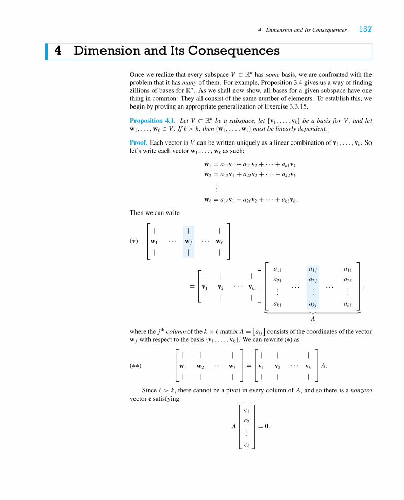
4 Dimension and Its Consequences 157
4 Dimension and Its Consequences
Once we realize that every subspace V ⊂ Rn has some basis, we are confronted with theproblem that it has many of them. For example, Proposition 3.4 gives us a way of findingzillions of bases for Rn. As we shall now show, all bases for a given subspace have onething in common: They all consist of the same number of elements. To establish this, webegin by proving an appropriate generalization of Exercise 3.3.15.
Proposition 4.1. Let V ⊂ Rn be a subspace, let {v1, . . . , vk} be a basis for V , and letw1, . . . ,w� ∈ V . If � > k, then {w1, . . . ,w�} must be linearly dependent.
Proof. Each vector in V can be written uniquely as a linear combination of v1, . . . , vk . Solet’s write each vector w1, . . . ,w� as such:
w1 = a11v1 + a21v2 + · · · + ak1vkw2 = a12v1 + a22v2 + · · · + ak2vk
...
w� = a1�v1 + a2�v2 + · · · + ak�vk.Then we can write
(∗)
⎡⎢⎢⎢⎣
|w1
|· · ·
|wj
|· · ·
|w�
|
⎤⎥⎥⎥⎦
=
⎡⎢⎢⎣
|v1
|
|v2
|· · ·
|vk
|
⎤⎥⎥⎦
⎡⎢⎢⎢⎢⎢⎢⎣
a11
a21
...
ak1
. . .
a1j
a2j
...
akj
. . .
a1�
a2�
...
ak�
⎤⎥⎥⎥⎥⎥⎥⎦
︸ ︷︷ ︸A
,
where the j th column of the k × �matrixA = [aij]
consists of the coordinates of the vectorwj with respect to the basis {v1, . . . , vk}. We can rewrite (∗) as
(∗∗)
⎡⎢⎢⎣
|w1
|
|w2
|· · ·
|w�
|
⎤⎥⎥⎦ =
⎡⎢⎢⎣
|v1
|
|v2
|· · ·
|vk
|
⎤⎥⎥⎦A.
Since � > k, there cannot be a pivot in every column of A, and so there is a nonzerovector c satisfying
A
⎡⎢⎢⎢⎢⎢⎣
c1
c2
...
c�
⎤⎥⎥⎥⎥⎥⎦
= 0.
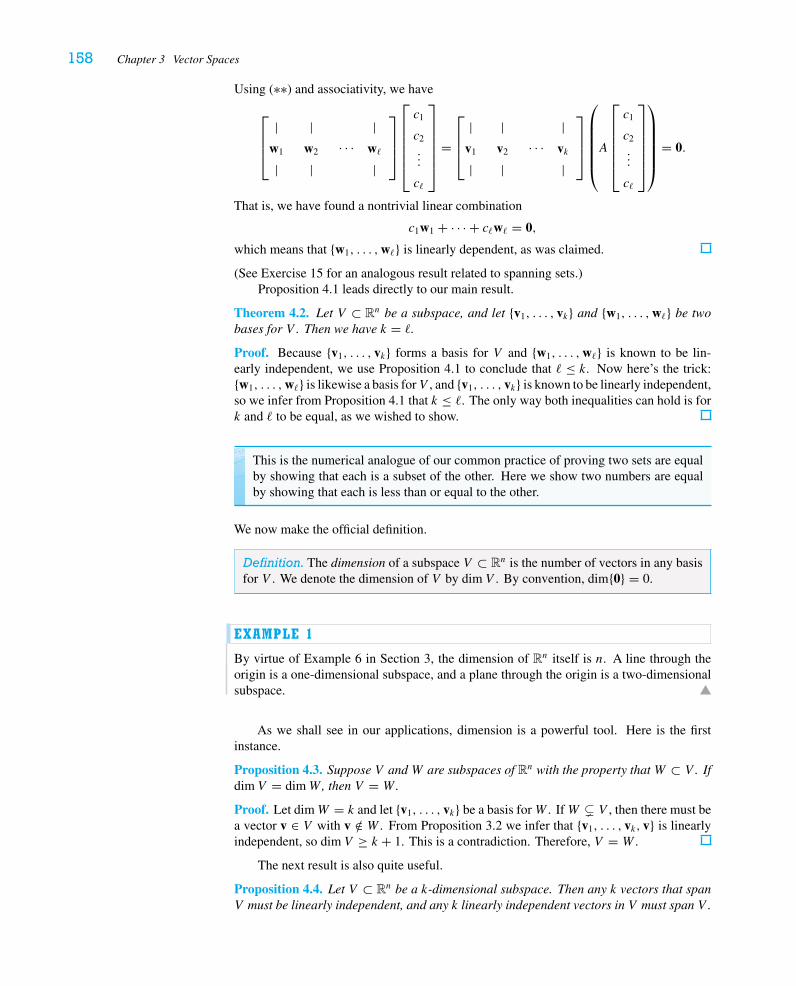
158 Chapter 3 Vector Spaces
Using (∗∗) and associativity, we have
⎡⎢⎢⎣
|w1
|
|w2
|· · ·
|w�
|
⎤⎥⎥⎦
⎡⎢⎢⎢⎢⎢⎣
c1
c2
...
c�
⎤⎥⎥⎥⎥⎥⎦
=
⎡⎢⎢⎣
|v1
|
|v2
|· · ·
|vk
|
⎤⎥⎥⎦
⎛⎜⎜⎜⎜⎜⎝A
⎡⎢⎢⎢⎢⎢⎣
c1
c2
...
c�
⎤⎥⎥⎥⎥⎥⎦
⎞⎟⎟⎟⎟⎟⎠
= 0.
That is, we have found a nontrivial linear combination
c1w1 + · · · + c�w� = 0,
which means that {w1, . . . ,w�} is linearly dependent, as was claimed.
(See Exercise 15 for an analogous result related to spanning sets.)Proposition 4.1 leads directly to our main result.
Theorem 4.2. Let V ⊂ Rn be a subspace, and let {v1, . . . , vk} and {w1, . . . ,w�} be twobases for V . Then we have k = �.
Proof. Because {v1, . . . , vk} forms a basis for V and {w1, . . . ,w�} is known to be lin-early independent, we use Proposition 4.1 to conclude that � ≤ k. Now here’s the trick:{w1, . . . ,w�} is likewise a basis forV , and {v1, . . . , vk} is known to be linearly independent,so we infer from Proposition 4.1 that k ≤ �. The only way both inequalities can hold is fork and � to be equal, as we wished to show.
This is the numerical analogue of our common practice of proving two sets are equalby showing that each is a subset of the other. Here we show two numbers are equalby showing that each is less than or equal to the other.
We now make the official definition.
Definition. The dimension of a subspace V ⊂ Rn is the number of vectors in any basisfor V . We denote the dimension of V by dim V . By convention, dim{0} = 0.
EXAMPLE 1
By virtue of Example 6 in Section 3, the dimension of Rn itself is n. A line through theorigin is a one-dimensional subspace, and a plane through the origin is a two-dimensionalsubspace.
As we shall see in our applications, dimension is a powerful tool. Here is the firstinstance.
Proposition 4.3. Suppose V andW are subspaces of Rn with the property thatW ⊂ V . Ifdim V = dimW , then V = W .
Proof. Let dimW = k and let {v1, . . . , vk} be a basis forW . IfW � V , then there must bea vector v ∈ V with v /∈ W . From Proposition 3.2 we infer that {v1, . . . , vk, v} is linearlyindependent, so dim V ≥ k + 1. This is a contradiction. Therefore, V = W .
The next result is also quite useful.
Proposition 4.4. Let V ⊂ Rn be a k-dimensional subspace. Then any k vectors that spanV must be linearly independent, and any k linearly independent vectors in V must span V .
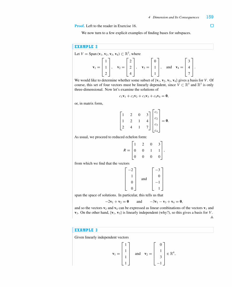
4 Dimension and Its Consequences 159
Proof. Left to the reader in Exercise 16.
We now turn to a few explicit examples of finding bases for subspaces.
EXAMPLE 2
Let V = Span (v1, v2, v3, v4) ⊂ R3, where
v1 =
⎡⎢⎢⎣
1
1
2
⎤⎥⎥⎦ , v2 =
⎡⎢⎢⎣
2
2
4
⎤⎥⎥⎦ , v3 =
⎡⎢⎢⎣
0
1
1
⎤⎥⎥⎦ , and v4 =
⎡⎢⎢⎣
3
4
7
⎤⎥⎥⎦ .
We would like to determine whether some subset of {v1, v2, v3, v4} gives a basis for V . Ofcourse, this set of four vectors must be linearly dependent, since V ⊂ R3 and R3 is onlythree-dimensional. Now let’s examine the solutions of
c1v1 + c2v2 + c3v3 + c4v4 = 0,
or, in matrix form,
⎡⎢⎢⎣
1 2 0 3
1 2 1 4
2 4 1 7
⎤⎥⎥⎦
⎡⎢⎢⎢⎢⎣
c1
c2
c3
c4
⎤⎥⎥⎥⎥⎦
= 0.
As usual, we proceed to reduced echelon form:
R =
⎡⎢⎢⎣
1 2 0 3
0 0 1 1
0 0 0 0
⎤⎥⎥⎦ ,
from which we find that the vectors⎡⎢⎢⎢⎢⎣
−2
1
0
0
⎤⎥⎥⎥⎥⎦
and
⎡⎢⎢⎢⎢⎣
−3
0
−1
1
⎤⎥⎥⎥⎥⎦
span the space of solutions. In particular, this tells us that
−2v1 + v2 = 0 and −3v1 − v3 + v4 = 0,
and so the vectors v2 and v4 can be expressed as linear combinations of the vectors v1 andv3. On the other hand, {v1, v3} is linearly independent (why?), so this gives a basis for V .
EXAMPLE 3
Given linearly independent vectors
v1 =
⎡⎢⎢⎢⎢⎣
1
1
1
1
⎤⎥⎥⎥⎥⎦
and v2 =
⎡⎢⎢⎢⎢⎣
0
1
3
−1
⎤⎥⎥⎥⎥⎦
∈ R4,
160 Chapter 3 Vector Spaces
we wish to find additional vectors v3, v4, . . . to make up a basis for R4 (as we shall seein Exercise 17, this is always possible). First of all, since dim R4 = 4, we know that onlytwo further vectors will be required. How should we find them? We might try guessing; amore methodical approach is suggested in Exercise 2. But here we try a more geometricsolution.
Let’s find a basis for the orthogonal complement of the subspace V spanned by v1 andv2. We consider the matrix A whose row vectors are v1 and v2:
A =[
1 1 1 1
0 1 3 −1
]�[
1 0 −2 2
0 1 3 −1
].
The vectors
v3 =
⎡⎢⎢⎢⎢⎣
2
−3
1
0
⎤⎥⎥⎥⎥⎦
and v4 =
⎡⎢⎢⎢⎢⎣
−2
1
0
1
⎤⎥⎥⎥⎥⎦
span N(A) (and therefore form a basis for N(A)—why?). By Proposition 2.2, {v3, v4} givesa basis for R(A)⊥ = V ⊥. We now give a geometric argument that {v1, v2, v3, v4} forms abasis for R4. (Alternatively, the reader could just check this in a straightforward numericalfashion.)
By Proposition 4.4, we need only check that {v1, v2, v3, v4} is linearly independent.Suppose, as usual, that
c1v1 + c2v2 + c3v3 + c4v4 = 0.
This means that
c1v1 + c2v2 = −(c3v3 + c4v4),
but the vector on the left hand side is in V and the vector on the right hand side is in V ⊥.By Exercise 3.1.10, only 0 can lie in both V and V ⊥, and so we conclude that
c1v1 + c2v2 = 0 and c3v3 + c4v4 = 0.
Now from the fact that {v1, v2} is linearly independent, we infer that c1 = c2 = 0, andfrom the fact that {v3, v4} is linearly independent, we infer that c3 = c4 = 0. In sum,{v1, v2, v3, v4} is linearly independent and therefore gives a basis for R4.
4.1 Back to the Four Fundamental SubspacesWe now return to the four fundamental subspaces associated to any matrix. We specify aprocedure for giving a basis for each of R(A), N(A), C(A), and N(AT). Their dimensionswill follow immediately. It may help the reader to compare this discussion with Example10 in Section 3; indeed, the theorem is best understood by working several examples.
Theorem 4.5. Let A be an m× n matrix. Let U and R, respectively, denote the echelonand reduced echelon form, respectively, of A, and write EA = U (so E is the product ofthe elementary matrices by which we reduce A to some echelon form).
1. The (transposes of the) nonzero rows of U (or of R) give a basis for R(A).
2. The vectors obtained by setting each free variable equal to 1 and the remainingfree variables equal to 0 in the general solution ofAx = 0 (which we read off fromRx = 0) give a basis for N(A).
4 Dimension and Its Consequences 161
3. The pivot columns of A (i.e., the columns of the original matrix A correspondingto the pivots in U ) give a basis for C(A).
4. The (transposes of the) rows of E that correspond to the zero rows of U give abasis for N(AT). (The same works with E′ if we write E′A = R.)
Proof. For simplicity of exposition, let’s assume that the reduced echelon form takes theshape
R =r
⎧⎪⎪⎨⎪⎪⎩
m−r{
⎡⎢⎢⎢⎢⎢⎢⎢⎣
1 b1,r+1 b1,r+2 · · · b1n
. . ....
.... . .
...
1 br,r+1 br,r+2 · · · brn
O O
⎤⎥⎥⎥⎥⎥⎥⎥⎦.
1. Since row operations are invertible, R(A) = R(U) (see Exercise 3.2.1). Clearlythe nonzero rows of U span R(U). Moreover, they are linearly independentbecause of the pivots. Let U1, . . . ,Ur denote the nonzero rows of U ; because ofour simplifying assumption on R, we know that the pivots of U occur in the firstr columns as well. Suppose now that
c1U1 + · · · + crUr = 0.
The first entry of the left-hand side is c1u11 (since the first entry of the vectorsU2, . . . ,Ur is 0 by definition of echelon form). Because u11 �= 0 by definition ofpivot, we must have c1 = 0. Continuing in this fashion, we find that c1 = c2 =· · · = cr = 0. In conclusion, {U1, . . . ,Ur} forms a basis for R(U) and hence forR(A).
2. Ax = 0 if and only if Rx = 0, which means that
x1 + b1,r+1xr+1 + b1,r+2xr+2 + · · · + b1nxn = 0
x2 + b2,r+1xr+1 + b2,r+2xr+2 + · · · + b2nxn = 0. . .
......
......
xr + br,r+1xr+1 + br,r+2xr+2 + · · · + brnxn = 0 .
Thus, an arbitrary element of N(A) can be written in the form
x =
⎡⎢⎢⎢⎢⎢⎢⎢⎢⎢⎢⎢⎢⎢⎢⎣
x1
...
xr
xr+1
xr+2
...
xn
⎤⎥⎥⎥⎥⎥⎥⎥⎥⎥⎥⎥⎥⎥⎥⎦
= xr+1
⎡⎢⎢⎢⎢⎢⎢⎢⎢⎢⎢⎢⎢⎢⎢⎣
−b1,r+1
...
−br,r+1
1
0...
0
⎤⎥⎥⎥⎥⎥⎥⎥⎥⎥⎥⎥⎥⎥⎥⎦
+ xr+2
⎡⎢⎢⎢⎢⎢⎢⎢⎢⎢⎢⎢⎢⎢⎢⎣
−b1,r+2
...
−br,r+2
0
1...
0
⎤⎥⎥⎥⎥⎥⎥⎥⎥⎥⎥⎥⎥⎥⎥⎦
+ · · · + xn
⎡⎢⎢⎢⎢⎢⎢⎢⎢⎢⎢⎢⎢⎢⎢⎣
−b1n
...
−brn0
0...
1
⎤⎥⎥⎥⎥⎥⎥⎥⎥⎥⎥⎥⎥⎥⎥⎦
.
162 Chapter 3 Vector Spaces
The assertion is then that the vectors⎡⎢⎢⎢⎢⎢⎢⎢⎢⎢⎢⎢⎢⎢⎢⎣
−b1,r+1
...
−br,r+1
1
0...
0
⎤⎥⎥⎥⎥⎥⎥⎥⎥⎥⎥⎥⎥⎥⎥⎦
,
⎡⎢⎢⎢⎢⎢⎢⎢⎢⎢⎢⎢⎢⎢⎢⎣
−b1,r+2
...
−br,r+2
0
1...
0
⎤⎥⎥⎥⎥⎥⎥⎥⎥⎥⎥⎥⎥⎥⎥⎦
, . . . ,
⎡⎢⎢⎢⎢⎢⎢⎢⎢⎢⎢⎢⎢⎢⎢⎣
−b1n
...
−brn0
0...
1
⎤⎥⎥⎥⎥⎥⎥⎥⎥⎥⎥⎥⎥⎥⎥⎦
give a basis for N(A). They obviously span N(A), because every vector in N(A)can be expressed as a linear combination of them. We need to check linear in-dependence: The key is the pattern of 1’s and 0’s in the free-variable “slots.”Suppose
0 =
⎡⎢⎢⎢⎢⎢⎢⎢⎢⎢⎢⎢⎢⎢⎢⎣
0...
0
0
0...
0
⎤⎥⎥⎥⎥⎥⎥⎥⎥⎥⎥⎥⎥⎥⎥⎦
= xr+1
⎡⎢⎢⎢⎢⎢⎢⎢⎢⎢⎢⎢⎢⎢⎢⎣
−b1,r+1
...
−br,r+1
1
0...
0
⎤⎥⎥⎥⎥⎥⎥⎥⎥⎥⎥⎥⎥⎥⎥⎦
+ xr+2
⎡⎢⎢⎢⎢⎢⎢⎢⎢⎢⎢⎢⎢⎢⎢⎣
−b1,r+2
...
−br,r+2
0
1...
0
⎤⎥⎥⎥⎥⎥⎥⎥⎥⎥⎥⎥⎥⎥⎥⎦
+ · · · + xn
⎡⎢⎢⎢⎢⎢⎢⎢⎢⎢⎢⎢⎢⎢⎢⎣
−b1n
...
−brn0
0...
1
⎤⎥⎥⎥⎥⎥⎥⎥⎥⎥⎥⎥⎥⎥⎥⎦
.
Then we get xr+1 = xr+2 = · · · = xn = 0, as required.
3. Let’s continue with the notational simplification that the pivots occur in the first rcolumns. Then we need to establish the fact that the first r column vectors of theoriginal matrixA give a basis for C(A). These vectors form a linearly independentset, since the only solution of
c1a1 + · · · + crar = 0
is c1 = c2 = · · · = cr = 0 (look only at the first r columns of A and the first rcolumns of R). It is more interesting to understand why a1, . . . , ar span C(A).Consider each of the basis vectors for N(A) given above: Each one gives us alinear combination of the column vectors of A that results in the zero vector. Inparticular, we find that
−b1,r+1a1 − · · · − br,r+1ar + ar+1 = 0
−b1,r+2a1 − · · · − br,r+2ar + ar+2 = 0...
.... . .
...
−b1na1 − · · · − brnar + an = 0 ,
from which we conclude that the vectors ar+1, . . . , an are all linear combinationsof a1, . . . , ar . It follows that C(A) is spanned by a1, . . . , ar , as required.
4. Recall that vectors in N(AT) correspond to ways of expressing the zero vectoras linear combinations of the rows of A. The first r rows of the echelon matrix
4 Dimension and Its Consequences 163
U form a linearly independent set, whereas the last m− r rows of U consist justof 0. Thus, we conclude from EA = U that the (transposes of the) last m− rrows of E span N(AT).5 But these vectors are linearly independent, because E isnonsingular. Thus, the vectors Er+1, . . . ,Em give a basis for N(AT).
Remark. Referring to our earlier discussion of (†) on p. 114 and our discussion in Sections2 and 3 of this chapter, we finally know that finding the constraint equations for C(A) willgive a basis for N(AT). It is also worth noting that to find bases for the four fundamentalsubspaces of the matrix A, we need only find the echelon form of A to deal with R(A)and C(A), the reduced echelon form of A to deal with N(A), and the echelon form of theaugmented matrix [A | b ] to deal with N(AT).
EXAMPLE 4
We want bases for R(A), N(A), C(A), and N(AT), given the matrix
A =
⎡⎢⎢⎢⎢⎣
1 1 2 0 0
0 1 1 −1 −1
1 1 2 1 2
2 1 3 −1 −3
⎤⎥⎥⎥⎥⎦.
We leave it to the reader to check that the reduced echelon form of A is
R =
⎡⎢⎢⎢⎢⎣
1 0 1 0 −1
0 1 1 0 1
0 0 0 1 2
0 0 0 0 0
⎤⎥⎥⎥⎥⎦
and that EA = U , where
E =
⎡⎢⎢⎢⎢⎣
1 0 0 0
0 1 0 0
−1 0 1 0
−4 1 2 1
⎤⎥⎥⎥⎥⎦
and U =
⎡⎢⎢⎢⎢⎣
1 1 2 0 0
0 1 1 −1 −1
0 0 0 1 2
0 0 0 0 0
⎤⎥⎥⎥⎥⎦.
Alternatively, the echelon form of the augmented matrix [A | b ] is
[EA | Eb ] =
⎡⎢⎢⎢⎢⎣
1 1 2 0 0 b1
0 1 1 −1 −1 b2
0 0 0 1 2 −b1 + b3
0 0 0 0 0 −4b1 + b2 + 2b3 + b4
⎤⎥⎥⎥⎥⎦.
5A vector not in their span would then give rise to a relation among the nonzero rows of U , which we knowto be linearly independent. A formal argument comes from writing A = E−1U , so ATx = 0 if and only ifUT
((ET)−1x
) = 0, and this happens if and only if x = ETy for some y ∈ N(UT). Since N(UT) is spanned bythe last m− r standard basis vectors for Rm, our claim follows.
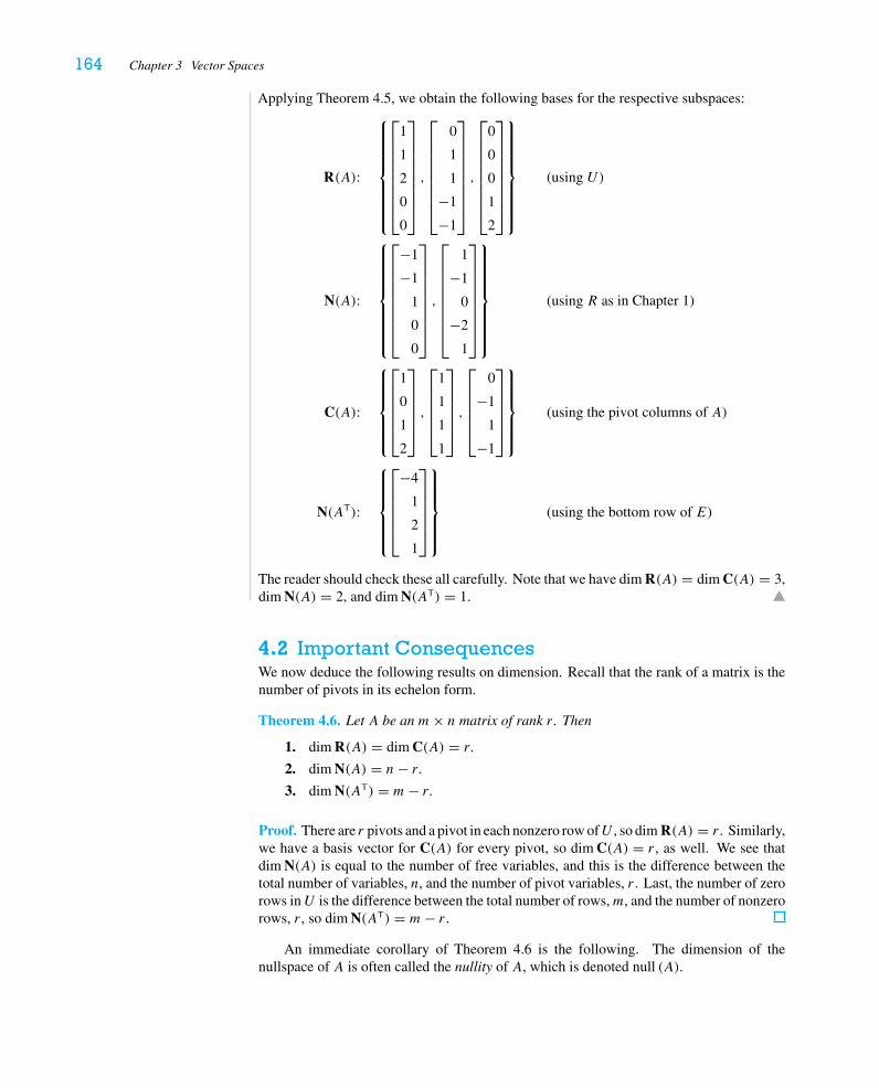
164 Chapter 3 Vector Spaces
Applying Theorem 4.5, we obtain the following bases for the respective subspaces:
R(A):
⎧⎪⎪⎪⎪⎪⎪⎪⎨⎪⎪⎪⎪⎪⎪⎪⎩
⎡⎢⎢⎢⎢⎢⎢⎢⎣
1
1
2
0
0
⎤⎥⎥⎥⎥⎥⎥⎥⎦,
⎡⎢⎢⎢⎢⎢⎢⎢⎣
0
1
1
−1
−1
⎤⎥⎥⎥⎥⎥⎥⎥⎦,
⎡⎢⎢⎢⎢⎢⎢⎢⎣
0
0
0
1
2
⎤⎥⎥⎥⎥⎥⎥⎥⎦
⎫⎪⎪⎪⎪⎪⎪⎪⎬⎪⎪⎪⎪⎪⎪⎪⎭
(using U )
N(A):
⎧⎪⎪⎪⎪⎪⎪⎪⎨⎪⎪⎪⎪⎪⎪⎪⎩
⎡⎢⎢⎢⎢⎢⎢⎢⎣
−1
−1
1
0
0
⎤⎥⎥⎥⎥⎥⎥⎥⎦,
⎡⎢⎢⎢⎢⎢⎢⎢⎣
1
−1
0
−2
1
⎤⎥⎥⎥⎥⎥⎥⎥⎦
⎫⎪⎪⎪⎪⎪⎪⎪⎬⎪⎪⎪⎪⎪⎪⎪⎭
(using R as in Chapter 1)
C(A):
⎧⎪⎪⎪⎪⎨⎪⎪⎪⎪⎩
⎡⎢⎢⎢⎢⎣
1
0
1
2
⎤⎥⎥⎥⎥⎦,
⎡⎢⎢⎢⎢⎣
1
1
1
1
⎤⎥⎥⎥⎥⎦,
⎡⎢⎢⎢⎢⎣
0
−1
1
−1
⎤⎥⎥⎥⎥⎦
⎫⎪⎪⎪⎪⎬⎪⎪⎪⎪⎭
(using the pivot columns of A)
N(AT):
⎧⎪⎪⎪⎪⎨⎪⎪⎪⎪⎩
⎡⎢⎢⎢⎢⎣
−4
1
2
1
⎤⎥⎥⎥⎥⎦
⎫⎪⎪⎪⎪⎬⎪⎪⎪⎪⎭
(using the bottom row of E)
The reader should check these all carefully. Note that we have dim R(A) = dim C(A) = 3,dim N(A) = 2, and dim N(AT) = 1.
4.2 Important ConsequencesWe now deduce the following results on dimension. Recall that the rank of a matrix is thenumber of pivots in its echelon form.
Theorem 4.6. Let A be an m× n matrix of rank r . Then
1. dim R(A) = dim C(A) = r .
2. dim N(A) = n− r .3. dim N(AT) = m− r .
Proof. There are r pivots and a pivot in each nonzero row ofU , so dim R(A) = r . Similarly,we have a basis vector for C(A) for every pivot, so dim C(A) = r , as well. We see thatdim N(A) is equal to the number of free variables, and this is the difference between thetotal number of variables, n, and the number of pivot variables, r . Last, the number of zerorows inU is the difference between the total number of rows,m, and the number of nonzerorows, r , so dim N(AT) = m− r .
An immediate corollary of Theorem 4.6 is the following. The dimension of thenullspace of A is often called the nullity of A, which is denoted null (A).
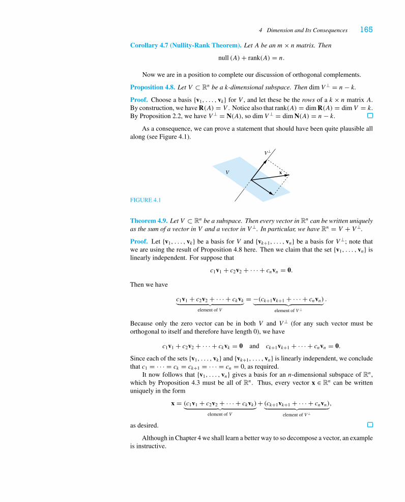
4 Dimension and Its Consequences 165
Corollary 4.7 (Nullity-Rank Theorem). Let A be an m× n matrix. Then
null (A)+ rank(A) = n.
Now we are in a position to complete our discussion of orthogonal complements.
Proposition 4.8. Let V ⊂ Rn be a k-dimensional subspace. Then dim V ⊥ = n− k.
Proof. Choose a basis {v1, . . . , vk} for V , and let these be the rows of a k × n matrix A.By construction, we have R(A) = V . Notice also that rank(A) = dim R(A) = dim V = k.By Proposition 2.2, we have V ⊥ = N(A), so dim V ⊥ = dim N(A) = n− k.
As a consequence, we can prove a statement that should have been quite plausible allalong (see Figure 4.1).
FIGURE 4.1
V x
V⊥
Theorem 4.9. Let V ⊂ Rn be a subspace. Then every vector in Rn can be written uniquelyas the sum of a vector in V and a vector in V ⊥. In particular, we have Rn = V + V ⊥.
Proof. Let {v1, . . . , vk} be a basis for V and {vk+1, . . . , vn} be a basis for V ⊥; note thatwe are using the result of Proposition 4.8 here. Then we claim that the set {v1, . . . , vn} islinearly independent. For suppose that
c1v1 + c2v2 + · · · + cnvn = 0.
Then we have
c1v1 + c2v2 + · · · + ckvk︸ ︷︷ ︸element of V
= −(ck+1vk+1 + · · · + cnvn)︸ ︷︷ ︸element of V ⊥
.
Because only the zero vector can be in both V and V ⊥ (for any such vector must beorthogonal to itself and therefore have length 0), we have
c1v1 + c2v2 + · · · + ckvk = 0 and ck+1vk+1 + · · · + cnvn = 0.
Since each of the sets {v1, . . . , vk} and {vk+1, . . . , vn} is linearly independent, we concludethat c1 = · · · = ck = ck+1 = · · · = cn = 0, as required.
It now follows that {v1, . . . , vn} gives a basis for an n-dimensional subspace of Rn,which by Proposition 4.3 must be all of Rn. Thus, every vector x ∈ Rn can be writtenuniquely in the form
x = (c1v1 + c2v2 + · · · + ckvk)︸ ︷︷ ︸element of V
+ (ck+1vk+1 + · · · + cnvn)︸ ︷︷ ︸element of V ⊥
,
as desired.
Although in Chapter 4 we shall learn a better way to so decompose a vector, an exampleis instructive.
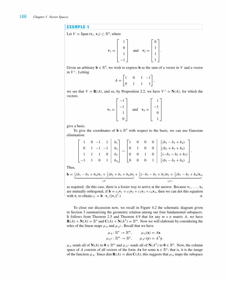
166 Chapter 3 Vector Spaces
EXAMPLE 5
Let V = Span (v1, v2) ⊂ R4, where
v1 =
⎡⎢⎢⎢⎢⎣
1
0
1
−1
⎤⎥⎥⎥⎥⎦
and v2 =
⎡⎢⎢⎢⎢⎣
0
1
1
1
⎤⎥⎥⎥⎥⎦.
Given an arbitrary b ∈ R4, we wish to express b as the sum of a vector in V and a vectorin V ⊥. Letting
A =[
1 0 1 −1
0 1 1 1
],
we see that V = R(A), and so, by Proposition 2.2, we have V ⊥ = N(A), for which thevectors
v3 =
⎡⎢⎢⎢⎢⎣
−1
−1
1
0
⎤⎥⎥⎥⎥⎦
and v4 =
⎡⎢⎢⎢⎢⎣
1
−1
0
1
⎤⎥⎥⎥⎥⎦
give a basis.To give the coordinates of b ∈ R4 with respect to the basis, we can use Gaussian
elimination:⎡⎢⎢⎢⎢⎣
1 0 −1 1 b1
0 1 −1 −1 b2
1 1 1 0 b3
−1 1 0 1 b4
⎤⎥⎥⎥⎥⎦
�
⎡⎢⎢⎢⎢⎣
1 0 0 0 13 (b1 − b3 + b4)
0 1 0 0 13 (b2 + b3 + b4)
0 0 1 0 13 (−b1 − b2 + b3)
0 0 0 1 13 (b1 − b2 + b4)
⎤⎥⎥⎥⎥⎦.
Thus,
b = 13 (b1 − b3 + b4)v1 + 1
3 (b2 + b3 + b4)v2︸ ︷︷ ︸∈V
+ 13 (−b1 − b2 + b3)v3 + 1
3 (b1 − b2 + b4)v4︸ ︷︷ ︸∈V ⊥
,
as required. (In this case, there is a foxier way to arrive at the answer. Because v1, . . . , v4
are mutually orthogonal, if b = c1v1 + c2v2 + c3v3 + c4v4, then we can dot this equationwith vi to obtain ci = b · vi/‖vi‖2.)
To close our discussion now, we recall in Figure 4.2 the schematic diagram givenin Section 3 summarizing the geometric relation among our four fundamental subspaces.It follows from Theorem 2.5 and Theorem 4.9 that for any m× n matrix A, we haveR(A)+ N(A) = Rn and C(A)+ N(AT) = Rm. Now we will elaborate by considering theroles of the linear maps μA and μAT . Recall that we have
μA : Rn → Rm, μA(x) = Ax
μAT : Rm → Rn, μAT(y) = ATy.
μA sends all of N(A) to 0 ∈ Rm and μAT sends all of N(AT) to 0 ∈ Rn. Now, the columnspace of A consists of all vectors of the form Ax for some x ∈ Rn; that is, it is the imageof the function μA. Since dim R(A) = dim C(A), this suggests that μA maps the subspace
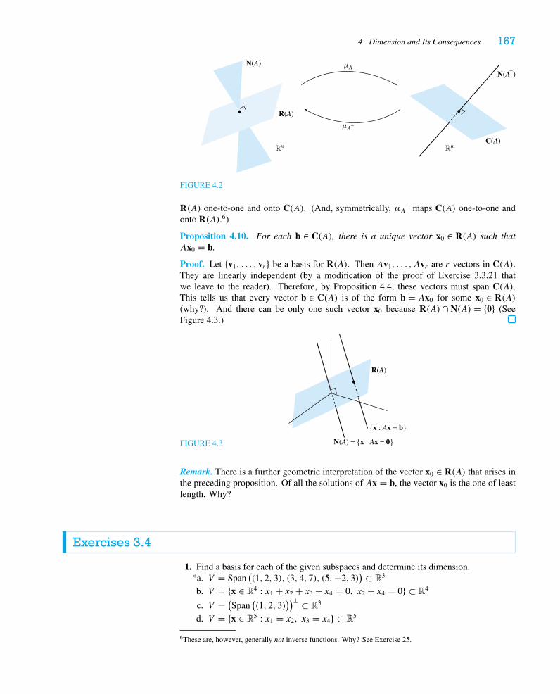
4 Dimension and Its Consequences 167
N(A)
R(A)
C(A)Rn Rm
μA
μA�
N(A�)
FIGURE 4.2
R(A) one-to-one and onto C(A). (And, symmetrically, μAT maps C(A) one-to-one andonto R(A).6)
Proposition 4.10. For each b ∈ C(A), there is a unique vector x0 ∈ R(A) such thatAx0 = b.
Proof. Let {v1, . . . , vr} be a basis for R(A). Then Av1, . . . , Avr are r vectors in C(A).They are linearly independent (by a modification of the proof of Exercise 3.3.21 thatwe leave to the reader). Therefore, by Proposition 4.4, these vectors must span C(A).This tells us that every vector b ∈ C(A) is of the form b = Ax0 for some x0 ∈ R(A)(why?). And there can be only one such vector x0 because R(A) ∩ N(A) = {0} (SeeFigure 4.3.)
FIGURE 4.3 N(A) = {x : Ax = 0}
{x : Ax = b}
R(A)
Remark. There is a further geometric interpretation of the vector x0 ∈ R(A) that arises inthe preceding proposition. Of all the solutions of Ax = b, the vector x0 is the one of leastlength. Why?
Exercises 3.4
1. Find a basis for each of the given subspaces and determine its dimension.a.∗ V = Span
((1, 2, 3), (3, 4, 7), (5,−2, 3)
) ⊂ R3
b. V = {x ∈ R4 : x1 + x2 + x3 + x4 = 0, x2 + x4 = 0} ⊂ R4
c. V = (Span
((1, 2, 3)
))⊥ ⊂ R3
d. V = {x ∈ R5 : x1 = x2, x3 = x4} ⊂ R5
6These are, however, generally not inverse functions. Why? See Exercise 25.
168 Chapter 3 Vector Spaces
2. In Example 3, we were given v1 =
⎡⎢⎢⎢⎣
1
1
1
1
⎤⎥⎥⎥⎦ , v2 =
⎡⎢⎢⎢⎣
0
1
3
−1
⎤⎥⎥⎥⎦ ∈ R4 and constructed v3, v4 so
that {v1, v2, v3, v4} gives a basis for R4. Here is an alternative construction: Considerthe collection of vectors v1, v2, e1, e2, e3, e4; these certainly span R4. Now use theapproach of Example 2 to find a basis {v1, v2, . . . }.
3. For each of the following matrices A, give bases for R(A), N(A), C(A), and N(AT).Check dimensions and orthogonality.
a. A =[
1 2 3
2 4 6
]
b. A =⎡⎢⎣
2 1 3
4 3 5
3 3 3
⎤⎥⎦
c. A =[
1 −2 1 0
2 −4 3 −1
]
d. A =
⎡⎢⎢⎢⎣
1 −1 1 1 0
1 0 2 1 1
0 2 2 2 0
−1 1 −1 0 −1
⎤⎥⎥⎥⎦
e. A =
⎡⎢⎢⎢⎣
1 1 0 1 −1
1 1 2 −1 1
2 2 2 0 0
−1 −1 2 −3 3
⎤⎥⎥⎥⎦
f.∗ A =
⎡⎢⎢⎢⎣
1 1 0 5 0 −1
0 1 1 3 −2 0
−1 2 3 4 1 −6
0 4 4 12 −1 −7
⎤⎥⎥⎥⎦
4. Find a basis for the intersection of the subspaces
V = Span((1, 0, 1, 1), (2, 1, 1, 2)
)and W = Span
((0, 1, 1, 0), (2, 0, 1, 2)
) ⊂ R4.
5.∗ Give a basis for the orthogonal complement of each of the following subspaces of R4.a. V = Span
((1, 0, 3, 4), (0, 1, 2,−5)
)b. W = {x ∈ R4 : x1 + 3x3 + 4x4 = 0, x2 + 2x3 − 5x4 = 0}
6. a. Give a basis for the orthogonal complement of the subspace V ⊂ R4 given by
V = {x ∈ R4 : x1 + x2 − 2x4 = 0, x1 − x2 − x3 + 6x4 = 0, x2 + x3 − 4x4 = 0}.b. Give a basis for the orthogonal complement of the subspace W ⊂ R4 spanned by(1, 1, 0,−2), (1,−1,−1, 6), and (0, 1, 1,−4).
c. Give a matrix B so that the subspaceW defined in part b can be written in the formW = N(B).
7. We saw in Exercise 2.5.13 that if them× nmatrixA has rank 1, then there are nonzerovectors u ∈ Rm and v ∈ Rn such that A = uvT. Describe the four fundamental sub-spaces of A in terms of u and v. (Hint: What are the columns of uvT?)
8. In each case, construct a matrix with the requisite properties or explain why no suchmatrix exists.
a.∗ The column space has basis
⎡⎢⎣
1
0
1
⎤⎥⎦, and the nullspace contains
⎡⎢⎣
1
2
0
⎤⎥⎦.
b. The nullspace contains
⎡⎢⎣
1
0
1
⎤⎥⎦,
⎡⎢⎣
−1
2
1
⎤⎥⎦, and the row space contains
⎡⎢⎣
1
1
−1
⎤⎥⎦.
4 Dimension and Its Consequences 169
c.∗ The column space has basis
⎡⎢⎣
1
0
1
⎤⎥⎦,
⎡⎢⎣
0
1
1
⎤⎥⎦, and the row space has basis
⎡⎢⎣
1
1
1
⎤⎥⎦,
⎡⎢⎣
2
0
1
⎤⎥⎦.
d. The column space and the nullspace both have basis
[1
0
].
e. The column space and the nullspace both have basis
⎡⎢⎣
1
0
0
⎤⎥⎦.
9. Given theLU decompositions of the following matricesA, give bases for R(A), N(A),C(A), and N(AT). (Do not multiply out!) Check dimensions and orthogonality.
a. A =[
1 0
2 1
][2 2 4
0 1 −1
]
b.∗ A =⎡⎢⎣
1 0 0
1 1 0
−2 0 1
⎤⎥⎦
⎡⎢⎣
1 1 2 1
0 0 2 −1
0 0 0 0
⎤⎥⎦
c. A =
⎡⎢⎢⎢⎣
1 0 0 0
−1 1 0 0
0 2 1 0
3 0 1 1
⎤⎥⎥⎥⎦
⎡⎢⎢⎢⎣
2 4 −2
0 0 3
0 0 0
0 0 0
⎤⎥⎥⎥⎦
10. According to Proposition 4.10, if A is an m× n matrix, then for each b ∈ C(A), thereis a unique x ∈ R(A) with Ax = b. In each case, give a formula for that x.
a. A =[
1 2 3
1 2 3
]b.∗ A =
[1 1 1
0 1 −1
]
11. Let A =[
1 −1 0 0
0 0 1 −1
].
a. Given any x ∈ R4, find u ∈ R(A) and v ∈ N(A) so that x = u + v.
b. Given b ∈ R2, give the unique element x ∈ R(A) so that Ax = b.
12. Let A be an n× n matrix. Prove that A is singular if and only if AT is singular.
13.∗ LetA be anm× nmatrix with rank r . SupposeA = BU , where U is in echelon form.Show that the first r columns of B give a basis for C(A). (In particular, if EA = U ,whereU is the echelon form ofA andE is the product of elementary matrices by whichwe reduce A to U , then the first r columns of E−1 give a basis for C(A).)
14. Recall from Exercise 3.1.13 that for any subspace V ⊂ Rn we have V ⊂ (V ⊥)⊥. Givealternative proofs of Proposition 3.6a.∗ by applying Proposition 4.3;
b. by applying Theorem 4.9 to prove that if x ∈ (V ⊥)⊥, then x ∈ V .
15. Let V ⊂ Rn be a subspace, let {v1, . . . , vk} be a basis for V , and let w1, . . . ,w� ∈ Vbe vectors such that Span (w1, . . . ,w�) = V . Prove that � ≥ k.
16. Prove Proposition 4.4. (Hint: Exercise 15 and Proposition 4.3 may be useful.)
17.� LetV ⊂ Rn be a subspace, and suppose you are given a linearly independent set of vec-tors {v1, . . . , vk} ⊂ V . Show that if dim V > k, then there are vectors vk+1, . . . , v� ∈ Vso that {v1, . . . , v�} forms a basis for V .
170 Chapter 3 Vector Spaces
18. SupposeV andW are subspaces of Rn andW ⊂ V . Prove that dimW ≤ dim V . (Hint:Start with a basis forW and apply Exercise 17.)
19. Suppose A is an n× n matrix, and let v1, . . . , vn ∈ Rn. Suppose {Av1, . . . , Avn} islinearly independent. Prove that A is nonsingular.
20. Continuing Exercise 3.3.23: Let U and V be subspaces of Rn. Prove that if U ∩ V ={0}, then dim(U + V ) = dimU + dim V .
21. Let U and V be subspaces of Rn. Prove that dim(U + V ) = dimU + dim V −dim(U ∩ V ). (Hint: This is a generalization of Exercise 20. Start with a basis forU ∩ V , and use Exercise 17.)
22. Continuing Exercise 3.2.10: Let A be an m× n matrix, and let B be an n× p matrix.a. Prove that rank(AB) ≤ rank(A). (Hint: Look at part b of Exercise 3.2.10.)
b. Prove that if n = p and B is nonsingular, then rank(AB) = rank(A).
c. Prove that rank(AB) ≤ rank(B). (Hint: Use part a of Exercise 3.2.10 and Theorem4.6.)
d. Prove that if m = n and A is nonsingular, then rank(AB) = rank(B).
e. Prove that if rank(AB) = n, then rank(A) = rank(B) = n.
23. a. LetA be anm× nmatrix, and let B be an n× p matrix. Show thatAB = O ⇐⇒C(B) ⊂ N(A).
b. Suppose A and B are 3 × 3 matrices of rank 2. Show that AB �= O.
c. Give examples of 3 × 3 matrices A and B of rank 2 so that AB has each possiblerank.
24.� Continuing Exercise 3.2.10: Let A be an m× n matrix.a. Use Theorem 2.5 to prove that N(ATA) = N(A). (Hint: If x ∈ N(ATA), thenAx ∈ C(A) ∩ N(AT).)
b. Prove that rank(A) = rank(ATA).
c. Prove that C(ATA) = C(AT).
25. In this exercise, we investigate the composition of functions μAT◦μA mapping R(A)to R(A), pursuing the discussion on p. 167.a. Suppose A is an m× n matrix. Show that ATA = In if and only if the column
vectors a1, . . . , an ∈ Rm are mutually orthogonal unit vectors.
b. SupposeA is anm× nmatrix of rank 1. Using the notation of Exercise 7, show thatATAx = x for each x ∈ R(A) if and only if ‖u‖‖v‖ = 1. Use this fact to show thatwe can write A = uvT, where ‖u‖ = ‖v‖ = 1. Interpret μA geometrically. (SeeExercise 4.4.22 for a generalization.)
26. Generalizing Exercise 3.2.13: Suppose A is an n× n matrix with the property thatrank(A) = rank(A2).a. Show that N(A2) = N(A).b. Prove that C(A) ∩ N(A) = {0}.c. Conclude that C(A)+ N(A) = Rn. (Hint: Use Exercise 20.)
5 A Graphic Example
In this brief section we show how the four fundamental subspaces (and their orthogonalityrelations) have a natural interpretation in elementary graph theory, a subject that has manyapplications in computer science, electronics, applied mathematics, and topology. We alsoreinterpret Kirchhoff’s laws from Section 6.3 of Chapter 1.
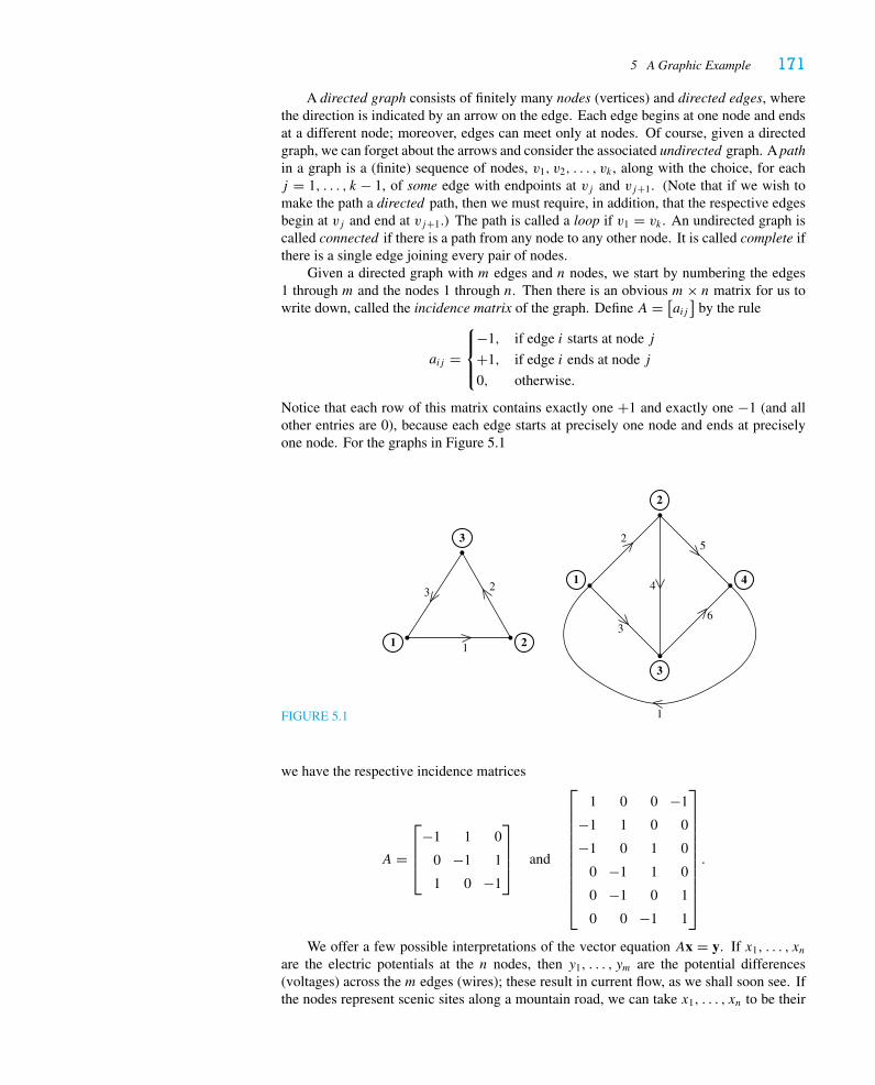
5 A Graphic Example 171
A directed graph consists of finitely many nodes (vertices) and directed edges, wherethe direction is indicated by an arrow on the edge. Each edge begins at one node and endsat a different node; moreover, edges can meet only at nodes. Of course, given a directedgraph, we can forget about the arrows and consider the associated undirected graph. A pathin a graph is a (finite) sequence of nodes, v1, v2, . . . , vk , along with the choice, for eachj = 1, . . . , k − 1, of some edge with endpoints at vj and vj+1. (Note that if we wish tomake the path a directed path, then we must require, in addition, that the respective edgesbegin at vj and end at vj+1.) The path is called a loop if v1 = vk . An undirected graph iscalled connected if there is a path from any node to any other node. It is called complete ifthere is a single edge joining every pair of nodes.
Given a directed graph with m edges and n nodes, we start by numbering the edges1 through m and the nodes 1 through n. Then there is an obvious m× n matrix for us towrite down, called the incidence matrix of the graph. Define A = [
aij]
by the rule
aij =
⎧⎪⎨⎪⎩
−1, if edge i starts at node j
+1, if edge i ends at node j
0, otherwise.
Notice that each row of this matrix contains exactly one +1 and exactly one −1 (and allother entries are 0), because each edge starts at precisely one node and ends at preciselyone node. For the graphs in Figure 5.1
FIGURE 5.1
1
23
1 2
3
1
2
3
1
2
3
4 4
5
6
we have the respective incidence matrices
A =
⎡⎢⎢⎣
−1 1 0
0 −1 1
1 0 −1
⎤⎥⎥⎦ and
⎡⎢⎢⎢⎢⎢⎢⎢⎢⎢⎢⎣
1 0 0 −1
−1 1 0 0
−1 0 1 0
0 −1 1 0
0 −1 0 1
0 0 −1 1
⎤⎥⎥⎥⎥⎥⎥⎥⎥⎥⎥⎦
.
We offer a few possible interpretations of the vector equation Ax = y. If x1, . . . , xnare the electric potentials at the n nodes, then y1, . . . , ym are the potential differences(voltages) across the m edges (wires); these result in current flow, as we shall soon see. Ifthe nodes represent scenic sites along a mountain road, we can take x1, . . . , xn to be their
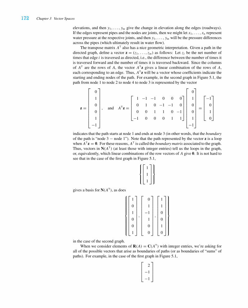
172 Chapter 3 Vector Spaces
elevations, and then y1, . . . , ym give the change in elevation along the edges (roadways).If the edges represent pipes and the nodes are joints, then we might let x1, . . . , xn representwater pressure at the respective joints, and then y1, . . . , ym will be the pressure differencesacross the pipes (which ultimately result in water flow).
The transpose matrix AT also has a nice geometric interpretation. Given a path in thedirected graph, define a vector z = (z1, . . . , zm) as follows: Let zi be the net number oftimes that edge i is traversed as directed, i.e., the difference between the number of times itis traversed forward and the number of times it is traversed backward. Since the columnsof AT are the rows of A, the vector ATz gives a linear combination of the rows of A,each corresponding to an edge. Thus, ATz will be a vector whose coefficients indicate thestarting and ending nodes of the path. For example, in the second graph in Figure 5.1, thepath from node 1 to node 2 to node 4 to node 3 is represented by the vector
z =
⎡⎢⎢⎢⎢⎢⎢⎢⎢⎢⎢⎣
0
1
0
0
1
−1
⎤⎥⎥⎥⎥⎥⎥⎥⎥⎥⎥⎦
, and ATz =
⎡⎢⎢⎢⎢⎣
1 −1 −1 0 0 0
0 1 0 −1 −1 0
0 0 1 1 0 −1
−1 0 0 0 1 1
⎤⎥⎥⎥⎥⎦
⎡⎢⎢⎢⎢⎢⎢⎢⎢⎢⎢⎣
0
1
0
0
1
−1
⎤⎥⎥⎥⎥⎥⎥⎥⎥⎥⎥⎦
=
⎡⎢⎢⎢⎢⎣
−1
0
1
0
⎤⎥⎥⎥⎥⎦
indicates that the path starts at node 1 and ends at node 3 (in other words, that the boundaryof the path is “node 3 − node 1”). Note that the path represented by the vector z is a loopwhenATz = 0. For these reasons,AT is called the boundary matrix associated to the graph.Thus, vectors in N(AT) (at least those with integer entries) tell us the loops in the graph,or, equivalently, which linear combinations of the row vectors of A give 0. It is not hard tosee that in the case of the first graph in Figure 5.1,
⎧⎪⎪⎨⎪⎪⎩
⎡⎢⎢⎣
1
1
1
⎤⎥⎥⎦
⎫⎪⎪⎬⎪⎪⎭
gives a basis for N(AT), as does⎧⎪⎪⎪⎪⎪⎪⎪⎪⎪⎪⎨⎪⎪⎪⎪⎪⎪⎪⎪⎪⎪⎩
⎡⎢⎢⎢⎢⎢⎢⎢⎢⎢⎢⎣
1
0
1
0
0
1
⎤⎥⎥⎥⎥⎥⎥⎥⎥⎥⎥⎦
,
⎡⎢⎢⎢⎢⎢⎢⎢⎢⎢⎢⎣
0
1
−1
1
0
0
⎤⎥⎥⎥⎥⎥⎥⎥⎥⎥⎥⎦
,
⎡⎢⎢⎢⎢⎢⎢⎢⎢⎢⎢⎣
1
1
0
0
1
0
⎤⎥⎥⎥⎥⎥⎥⎥⎥⎥⎥⎦
⎫⎪⎪⎪⎪⎪⎪⎪⎪⎪⎪⎬⎪⎪⎪⎪⎪⎪⎪⎪⎪⎪⎭
in the case of the second graph.When we consider elements of R(A) = C(AT) with integer entries, we’re asking for
all of the possible vectors that arise as boundaries of paths (or as boundaries of “sums” ofpaths). For example, in the case of the first graph in Figure 5.1,
⎡⎢⎢⎣
2
−1
−1
⎤⎥⎥⎦
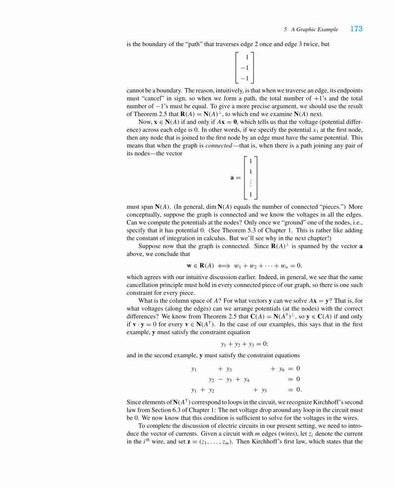
5 A Graphic Example 173
is the boundary of the “path” that traverses edge 2 once and edge 3 twice, but⎡⎢⎢⎣
1
−1
−1
⎤⎥⎥⎦
cannot be a boundary. The reason, intuitively, is that when we traverse an edge, its endpointsmust “cancel” in sign, so when we form a path, the total number of +1’s and the totalnumber of −1’s must be equal. To give a more precise argument, we should use the resultof Theorem 2.5 that R(A) = N(A)⊥, to which end we examine N(A) next.
Now, x ∈ N(A) if and only if Ax = 0, which tells us that the voltage (potential differ-ence) across each edge is 0. In other words, if we specify the potential x1 at the first node,then any node that is joined to the first node by an edge must have the same potential. Thismeans that when the graph is connected—that is, when there is a path joining any pair ofits nodes—the vector
a =
⎡⎢⎢⎢⎢⎢⎣
1
1...
1
⎤⎥⎥⎥⎥⎥⎦
must span N(A). (In general, dim N(A) equals the number of connected “pieces.”) Moreconceptually, suppose the graph is connected and we know the voltages in all the edges.Can we compute the potentials at the nodes? Only once we “ground” one of the nodes, i.e.,specify that it has potential 0. (See Theorem 5.3 of Chapter 1. This is rather like addingthe constant of integration in calculus. But we’ll see why in the next chapter!)
Suppose now that the graph is connected. Since R(A)⊥ is spanned by the vector aabove, we conclude that
w ∈ R(A) ⇐⇒ w1 + w2 + · · · + wn = 0,
which agrees with our intuitive discussion earlier. Indeed, in general, we see that the samecancellation principle must hold in every connected piece of our graph, so there is one suchconstraint for every piece.
What is the column space of A? For what vectors y can we solve Ax = y? That is, forwhat voltages (along the edges) can we arrange potentials (at the nodes) with the correctdifferences? We know from Theorem 2.5 that C(A) = N(AT)⊥, so y ∈ C(A) if and onlyif v · y = 0 for every v ∈ N(AT). In the case of our examples, this says that in the firstexample, y must satisfy the constraint equation
y1 + y2 + y3 = 0;and in the second example, y must satisfy the constraint equations
y1 + y3 + y6 = 0
y2 − y3 + y4 = 0
y1 + y2 + y5 = 0 .
Since elements of N(AT) correspond to loops in the circuit, we recognize Kirchhoff’s secondlaw from Section 6.3 of Chapter 1: The net voltage drop around any loop in the circuit mustbe 0. We now know that this condition is sufficient to solve for the voltages in the wires.
To complete the discussion of electric circuits in our present setting, we need to intro-duce the vector of currents. Given a circuit with m edges (wires), let zi denote the currentin the i th wire, and set z = (z1, . . . , zm). Then Kirchhoff’s first law, which states that the
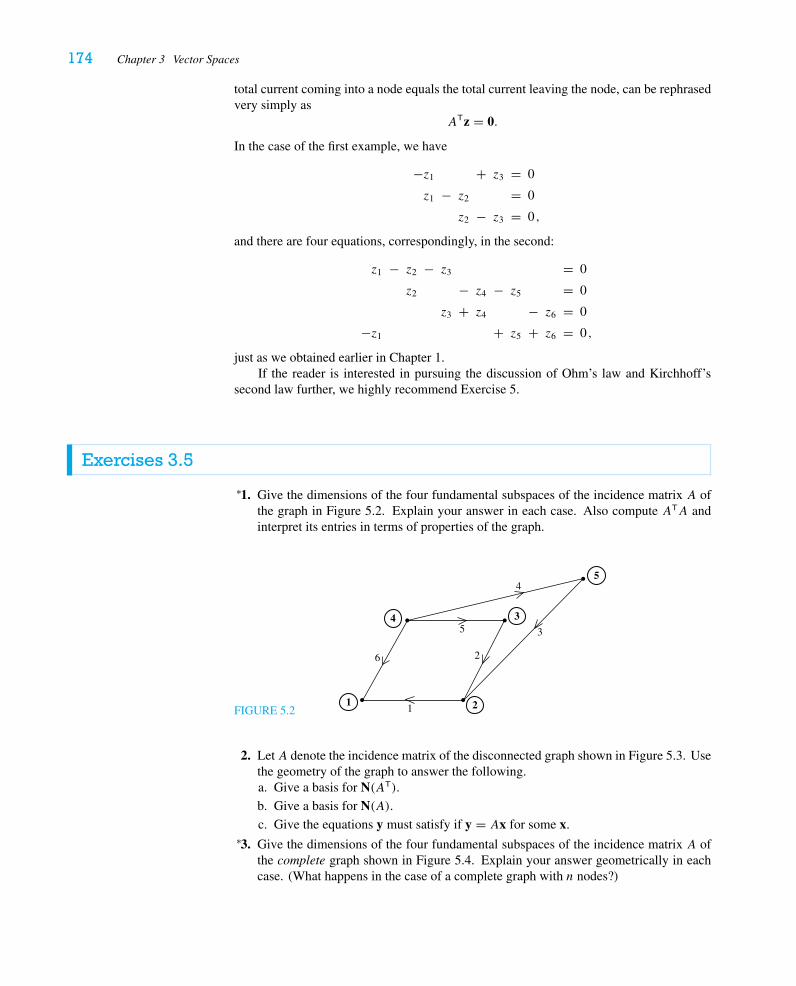
174 Chapter 3 Vector Spaces
total current coming into a node equals the total current leaving the node, can be rephrasedvery simply as
ATz = 0.
In the case of the first example, we have
−z1 + z3 = 0
z1 − z2 = 0
z2 − z3 = 0 ,
and there are four equations, correspondingly, in the second:
z1 − z2 − z3 = 0
z2 − z4 − z5 = 0
z3 + z4 − z6 = 0
−z1 + z5 + z6 = 0 ,
just as we obtained earlier in Chapter 1.If the reader is interested in pursuing the discussion of Ohm’s law and Kirchhoff’s
second law further, we highly recommend Exercise 5.
Exercises 3.5
1.∗ Give the dimensions of the four fundamental subspaces of the incidence matrix A ofthe graph in Figure 5.2. Explain your answer in each case. Also compute ATA andinterpret its entries in terms of properties of the graph.
FIGURE 5.2 1
2
3
4
5
1 2
34
5
6
2. Let A denote the incidence matrix of the disconnected graph shown in Figure 5.3. Usethe geometry of the graph to answer the following.a. Give a basis for N(AT).
b. Give a basis for N(A).c. Give the equations y must satisfy if y = Ax for some x.
3.∗ Give the dimensions of the four fundamental subspaces of the incidence matrix A ofthe complete graph shown in Figure 5.4. Explain your answer geometrically in eachcase. (What happens in the case of a complete graph with n nodes?)
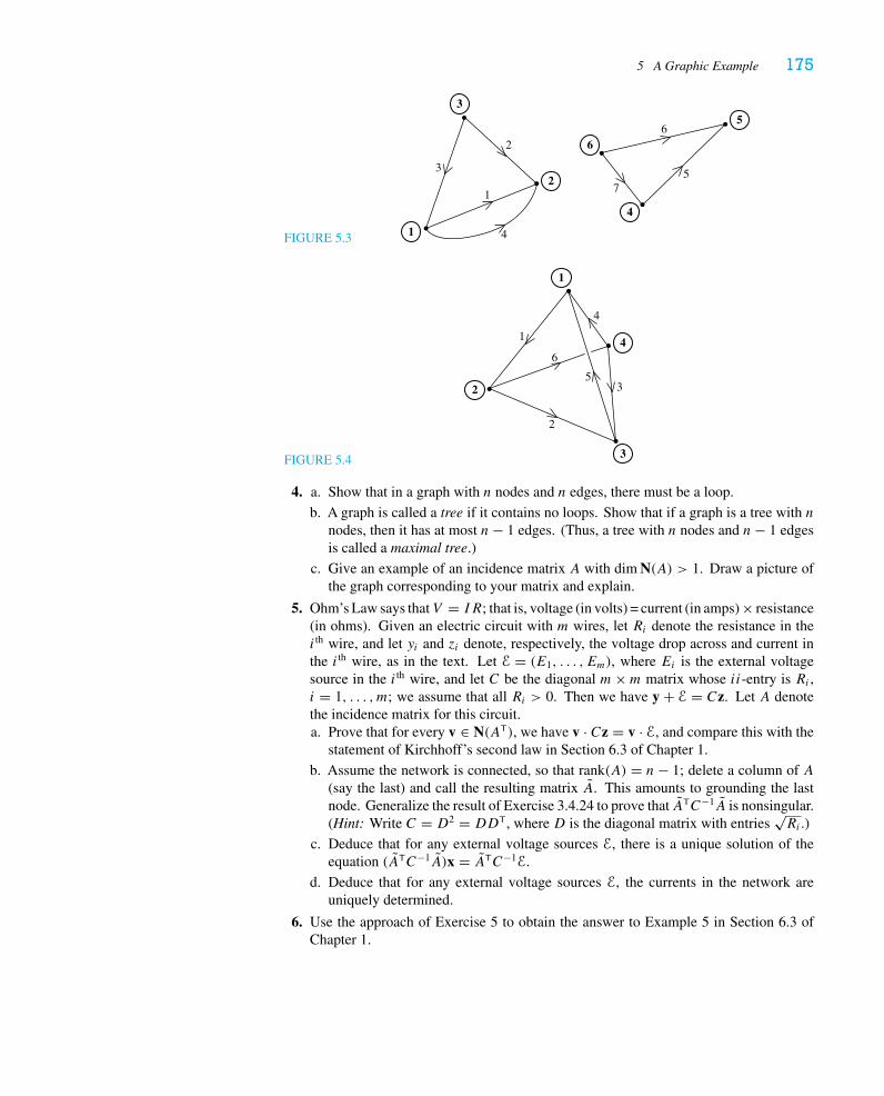
5 A Graphic Example 175
FIGURE 5.3
1
2
3
4
5
6
1
2
3
4
5
6
7
FIGURE 5.4
1
2
3
4
5
6
3
4
2
1
4. a. Show that in a graph with n nodes and n edges, there must be a loop.
b. A graph is called a tree if it contains no loops. Show that if a graph is a tree with nnodes, then it has at most n− 1 edges. (Thus, a tree with n nodes and n− 1 edgesis called a maximal tree.)
c. Give an example of an incidence matrix A with dim N(A) > 1. Draw a picture ofthe graph corresponding to your matrix and explain.
5. Ohm’s Law says thatV = IR; that is, voltage (in volts) = current (in amps) × resistance(in ohms). Given an electric circuit with m wires, let Ri denote the resistance in thei th wire, and let yi and zi denote, respectively, the voltage drop across and current inthe i th wire, as in the text. Let E = (E1, . . . , Em), where Ei is the external voltagesource in the i th wire, and let C be the diagonal m×m matrix whose ii-entry is Ri ,i = 1, . . . , m; we assume that all Ri > 0. Then we have y + E = Cz. Let A denotethe incidence matrix for this circuit.a. Prove that for every v ∈ N(AT), we have v · Cz = v · E, and compare this with the
statement of Kirchhoff’s second law in Section 6.3 of Chapter 1.
b. Assume the network is connected, so that rank(A) = n− 1; delete a column of A(say the last) and call the resulting matrix A. This amounts to grounding the lastnode. Generalize the result of Exercise 3.4.24 to prove that ATC−1A is nonsingular.(Hint: Write C = D2 = DDT, where D is the diagonal matrix with entries
√Ri .)
c. Deduce that for any external voltage sources E, there is a unique solution of theequation (ATC−1A)x = ATC−1E.
d. Deduce that for any external voltage sources E, the currents in the network areuniquely determined.
6. Use the approach of Exercise 5 to obtain the answer to Example 5 in Section 6.3 ofChapter 1.
176 Chapter 3 Vector Spaces
6 Abstract Vector Spaces
We have seen throughout this chapter that subspaces of Rn behave algebraically much thesame way as Rn itself. They are endowed with two operations: vector addition and scalarmultiplication. But there are lots of other interesting collections of objects—which do not inany obvious way live in some Euclidean space Rn—that have the same algebraic properties.In order to study some of these collections and see some of their applications, we first makethe following general definition.
Definition.A (real) vector space V is a set that is equipped with two operations, vectoraddition and scalar multiplication, which satisfy the following properties:
1. For all u, v ∈ V , u + v = v + u.
2. For all u, v,w ∈ V , (u + v)+ w = u + (v + w).
3. There is a vector 0 ∈ V (the zero vector) such that 0 + u = u for all u ∈ V .
4. For each u ∈ V , there is a vector −u ∈ V such that u + (−u) = 0.
5. For all c, d ∈ R and u ∈ V , c(du) = (cd)u.
6. For all c ∈ R and u, v ∈ V , c(u + v) = cu + cv.
7. For all c, d ∈ R and u ∈ V , (c + d)u = cu + du.
8. For all u ∈ V , 1u = u.
EXAMPLE 1
(a) Rn is, of course, a vector space, as is any subspace of Rn.
(b) The empty set is not a vector space, since it does not satisfy condition (3) of thedefinition. All the remaining criteria are satisfied “by default.”
(c) Let Mm×n denote the set of all m× n matrices. As we’ve seen in Proposition 1.1 ofChapter 2, Mm×n is a vector space, using the operations of matrix addition and scalarmultiplication we’ve already defined. The zero “vector” is the zero matrix O.
(d) Let F(I) denote the collection of all real-valued functions defined on some intervalI ⊂ R. If f ∈ F(I) and c ∈ R, then we can define a new function cf ∈ F(I) bymultiplying the value of f at each point by the scalar c:
(cf )(t) = c f (t) for each t ∈ I.Similarly, iff, g ∈ F(I), then we can define the new functionf + g ∈ F(I) by addingthe values of f and g at each point:
(f + g)(t) = f (t)+ g(t) for each t ∈ I.By these formulas we define scalar multiplication and vector addition in F(I). Thezero “vector” in F(I) is the zero function, whose value at each point is 0:
0(t) = 0 for each t ∈ I.The various properties of a vector space follow from the corresponding properties ofthe real numbers (because everything is defined in terms of the values of the functionat every point t). Since an element of F(I) is a function, F(I) is often called a functionspace.
6 Abstract Vector Spaces 177
(e) Let Rω denote the collection of all infinite sequences of real numbers. That is, anelement of Rω looks like
x = (x1, x2, x3, . . . ),
where all the xi’s are real numbers. Operations are defined in the obvious way: Ifc ∈ R, then
cx = (cx1, cx2, cx3, . . . ),
and if y = (y1, y2, y3, . . . ) ∈ Rω, we define addition by
x + y = (x1 + y1, x2 + y2, x3 + y3, . . . ).
As we did with Rn, we can define subspaces of a general vector space, and they toocan be considered as vector spaces in their own right.
Definition. Let V be a vector space. We sayW ⊂ V is a subspace if
1. 0 ∈ W (the zero vector belongs toW );
2. whenever v ∈ W and c ∈ R, we have cv ∈ W (W is closed under scalar mul-tiplication);
3. whenever v,w ∈ W , we have v + w ∈ W (W is closed under addition).
Proposition 6.1. If V is a vector space andW ⊂ V is a subspace, thenW is also a vectorspace.
Proof. We need to check that W satisfies the eight properties in the definition. Thecrucial point is that the definition of subspace ensures that when we perform vector additionor scalar multiplication starting with vector(s) in W , the result again lies in W . All thealgebraic properties hold in W because they already hold in V . Only one subtle pointshould be checked: Given w ∈ W , we know w has an additive inverse −w in V , but whymust this vector lie inW? We leave this to the reader to check (but, for a hint, see part b ofExercise 1).
EXAMPLE 2
Consider the vector space Mn×n of square matrices. Then the following are subspaces:
U = {upper triangular matrices}D = {diagonal matrices}L = {lower triangular matrices}.
We ask the reader to check the details in Exercise 5.
EXAMPLE 3
Fix an n× nmatrixM and letW = {A ∈ Mn×n : AM = MA}. This is the set of matricesthat commute withM . We ask whetherW is a subspace of Mn×n. Since OM = O = MO,it follows that O ∈ W . If c is a scalar and A ∈ W , then (cA)M = c(AM) = c(MA) =M(cA), so cA ∈ W as well. Last, suppose A,B ∈ W . Then (A+ B)M = AM + BM =MA+MB = M(A+ B), so A+ B ∈ W , as we needed. This completes the verificationthatW is a subspace of Mn×n.
178 Chapter 3 Vector Spaces
EXAMPLE 4
There are many interesting—and extremely important—subspaces of F(I). The spaceC0(I) of continuous functions on I is a subspace because of the important result fromcalculus that states: If f is a continuous function, then so is cf for any c ∈ R; and if f andg are continuous functions, then so is f + g. In addition, the zero function is continuous.
The space D(I) of differentiable functions is a subspace of C0(I). First, every differ-entiable function is continuous. Next, we have an analogous result from calculus that states:If f is a differentiable function, then so is cf for any c ∈ R; and if f and g are differentiablefunctions, then so is f + g. Likewise, the zero function is differentiable. Indeed, we knowmore from our calculus class. We have formulas for the relevant derivatives:
(cf )′ = cf ′ and (f + g)′ = f ′ + g′,
which will be important in Chapter 4.Mathematicians tend to concentrate on the subspace C1(I) ⊂ D(I) of continuously
differentiable functions. (A function f is continuously differentiable if its derivative f ′ isa continuous function.) They then move down the hierarchy:
C0(I) ⊃ C1(I) ⊃ C2(I) ⊃ C3(I) ⊃ · · · ⊃ Ck(I) ⊃ Ck+1(I) ⊃ · · · ⊃ C∞(I),where Ck(I) is the collection of functions on I that are (at least) k times continuouslydifferentiable and C∞(I) is the collection of functions on I that are infinitely differentiable.The reader who’s had some experience with mathematical induction can easily prove theseare all subspaces.
EXAMPLE 5
LetW ⊂ Rω denote the set of all sequences that are eventually 0. That is, let
W = {x ∈ Rω : there is a positive integer n such that xk = 0 for all k > n}.Then we claim thatW is a subspace of Rω.
Clearly, 0 ∈ W . If x ∈ W , then there is an integer n such that xk = 0 for all k > n, so,for any scalar c, we know that cxk = 0 for all k > n. Therefore, the kth coordinate of cx is0 for all k > n and so cx ∈ W as well. Now, suppose x and y ∈ W . Then there are integersn and p such that xk = 0 for all k > n and yk = 0 for all k > p. It follows that xk + yk = 0for all k larger than both n and p. (Officially, we write this as k > max(n, p).) Therefore,x + y ∈ W .
Of particular importance to us here is the vector space P of polynomials. Recall thata polynomial p of degree k is a function of the form
p(t) = aktk + ak−1t
k−1 + · · · + a1t + a0,
where a0, a1, . . . , ak are real numbers and ak �= 0. If c ∈ R, then the scalar multiple cp isgiven by the formula
(cp)(t) = caktk + cak−1t
k−1 + · · · + ca1t + ca0.
If q is another polynomial of degree k, say
q(t) = bktk + bk−1t
k−1 + · · · + b1t + b0,
then the sum p + q is again a polynomial:
(p + q)(t) = (ak + bk)tk + (ak−1 + bk−1)tk−1 + · · · + (a1 + b1)t + (a0 + b0).

6 Abstract Vector Spaces 179
But be careful! The sum of two polynomials of degree k may well have lesser degree.(For example, let p(t) = t2 − 2t + 3 and q(t) = −t2 + t − 1.) Thus, it is also natural toconsider the subspacesPk of polynomials of degree at most k, including the zero polynomial.We will return to study the spaces Pk shortly.
It is easy to extend the notions of span, linear independence, basis, and dimension tothe setting of general vector spaces. We briefly restate the definitions here to be sure.
Definition. Let V be a vector space and let v1, . . . , vk ∈ V . Then the span of v1, . . . , vkis the set
Span (v1, . . . , vk) = {c1v1 + c2v2 + · · · + ckvk : c1, c2, . . . , ck ∈ R}.We say {v1, . . . , vk} is linearly independent if
c1v1 + c2v2 + · · · + ckvk = 0 only when c1 = c2 = · · · = ck = 0.
Otherwise, we say {v1, . . . , vk} is linearly dependent.We say {v1, . . . , vk} is a basis for V if
(i) v1, . . . , vk span V , i.e., V = Span (v1, . . . , vk), and
(ii) {v1, . . . , vk} is linearly independent.
EXAMPLE 6
Consider the polynomials p1(t) = t + 1, p2(t) = t2 + 2, and p3(t) = t2 − t . We want todecide whether {p1, p2, p3} ⊂ P is a linearly independent set of vectors. Suppose c1p1 +c2p2 + c3p3 = 0. This means
c1(t + 1)+ c2(t2 + 2)+ c3(t
2 − t) = 0 for all t.
By specifying different values of t , we may obtain a homogeneous system of linear equationsin the variables c1, c2, and c3:
t = −1 : 3c2 + 2c3 = 0
t = 0 : c1 + 2c2 = 0
t = 1 : 2c1 + 3c2 = 0 .
We leave it to the reader to check that the only solution is c1 = c2 = c3 = 0, and so thefunctions p1, p2, and p3 do indeed form a linearly independent set.
At this point, we stop to make one new definition.
Definition. Let V be a vector space. We say V is finite-dimensional if there are aninteger k and vectors v1, . . . , vk that form a basis for V . A vector space that is notfinite-dimensional is called infinite-dimensional.
EXAMPLE 7
Observe that for any positive integer n, Rn is naturally a subspace of Rω: Given a vec-tor (x1, . . . , xn) ∈ Rn, merely consider the corresponding vector (x1, . . . , xn, 0, . . . ) ∈ Rω.Since Rn is a subspace of Rω for every positive integer n, Rω contains an n-dimensional
180 Chapter 3 Vector Spaces
subspace for every positive integer n. It follows that Rω is infinite-dimensional. Whatabout the subspaceW of sequences that are eventually 0, defined in Example 5? Well, thesame argument is valid, since every Rn is also a subspace ofW .
The reader should check that all the results of Sections 1, 2, 3, and 4 that applied tosubspaces of Rn apply to any finite-dimensional vector space. The one argument that trulyrelied on coordinates was the proof of Proposition 4.1, which allowed us to conclude thatdimension is well-defined. We now give a proof that works in general.
Proposition 6.2. Let V be a finite-dimensional vector space and suppose {v1, . . . , vk} is abasis for V . If w1, . . . ,w� ∈ V and � > k, then {w1, . . . ,w�} must be linearly dependent.
Proof. As in the proof of Proposition 4.1, we write
w1 = a11v1 + a21v2 + · · · + ak1vkw2 = a12v1 + a22v2 + · · · + ak2vk
...
w� = a1�v1 + a2�v2 + · · · + ak�vkand form the k × � matrix A = [
aij]. As before, since � > k, there is a nonzero vector
c ∈ N(A), and
�∑j=1
cjwj =�∑j=1
cj
( k∑i=1
aijvi
)=
k∑i=1
( �∑j=1
aij cj
)vi = 0.
Consequently, there is a nontrivial relation among w1, . . . ,w�, as we were to show.
Now Theorem 4.2 follows just as before, and we see that the notion of dimension makessense in arbitrary vector spaces. We will see in a moment that we’ve already encounteredseveral infinite-dimensional vector spaces.
We next consider the dimension of Pk , the vector space of polynomials of degreeat most k. Let f0(t) = 1, f1(t) = t , f2(t) = t2, . . . , fk(t) = tk .
Proposition 6.3. The set {f0, f1, . . . , fk} is a basis for Pk . Thus, Pk is a (k + 1)-dimensional vector space.
Proof. We first check that f0, . . . , fk span Pk . Suppose p ∈ Pk; then for appropriatea0, a1, . . . , ak ∈ R, we have
p(t) = aktk + ak−1t
k−1 + · · · + a1t + a0
= akfk(t)+ ak−1fk−1(t)+ · · · + a1f1(t)+ a0f0(t),
sop = akfk + ak−1fk−1 + · · · + a1f1 + a0f0
is a linear combination of f0, f1, . . . , fk , as required.How do we see that the functions f0, f1, . . . , fk form a linearly independent set?
Suppose c0f0 + c1f1 + · · · + ckfk = 0. This means that
p(t) = c0 + c1t + c2t2 + · · · + cktk = 0 for every t ∈ R.
Now, it is a fact from basic algebra (see Exercise 11) that a polynomial of degree ≤ k canhave at most k roots, unless it is the zero polynomial. Since p(t) = 0 for all t ∈ R, p mustbe the zero polynomial; i.e., c0 = c1 = · · · = ck = 0, as required.
Here is an example that indicates an alternative proof of the linear independence.
6 Abstract Vector Spaces 181
EXAMPLE 8
We will show directly that {f0, f1, f2, f3} is linearly independent. Suppose c0f0 + c1f1 +c2f2 + c3f3 = 0. We must show that c0 = c1 = c2 = c3 = 0. Let
p(t) = c0f0(t)+ c1f1(t)+ c2f2(t)+ c3f3(t) = c0 + c1t + c2t2 + c3t
3.
Since p(t) = 0 for all t , it follows that p(0) = 0, so c0 = 0. Since polynomials are (in-finitely) differentiable, and since the derivative of the zero function is the zero function, weobtain
p′(t) = c1 + 2c2t + 3c3t2 = 0 for all t.
Once again, we have p′(0) = 0, and so c1 = 0. Similarly,
p′′(t) = 2c2 + 6c3t = 0 for all t and p′′′(t) = 6c3 = 0 for all t,
and so, evaluating at 0 once again, we have c2 = c3 = 0. We conclude that c0 = c1 = c2 =c3 = 0, so {f0, f1, f2, f3} is linearly independent.
Since dim Pk = k + 1 for each nonnegative integer k, we see from the relations
P0 � P1 � P2 � · · · � Pk � · · · � P � C∞(R) � · · · � C2(R) � C1(R) � C0(R),
that P , C∞(R), and Ck(R) all contain subspaces of arbitrarily large dimension. This meansthat P must be infinite-dimensional, and hence so must C∞(R) and Ck(R) for every k ≥ 0.
EXAMPLE 9
Let V = {f ∈ C1(R) : f ′(t) = f (t) for all t ∈ R}. V is a subspace of C1(R), since
1. the zero function clearly has this property;
2. if f ∈ V and c ∈ R, then (cf )′(t) = cf ′(t) = cf (t) = (cf )(t), so cf ∈ V ;
3. iff, g ∈ V , then (f + g)′(t) = f ′(t)+ g′(t) = f (t)+ g(t) = (f + g)(t), sof +g ∈ V .
A rather obvious element of V is the function f1(t) = et . We claim that f1 spans V andhence provides a basis for V . To see this, let f be an arbitrary element of V and considerthe function g(t) = f (t)e−t . Then, differentiating, we have
g′(t) = f ′(t)e−t − f (t)e−t = (f ′(t)− f (t))e−t = 0 for all t ∈ R,
and so, by the Mean Value Theorem in differential calculus, g(t) = c for some c ∈ R. Thus,f (t)e−t = c and so f (t) = cet , as required.
We will explore the relation between linear algebra and differential equations further inSection 3 of Chapter 7.
We have not yet mentioned the dot product in the setting of abstract vector spaces.
Definition. Let V be a real vector space. We say V is an inner product space if forevery pair of elements u, v ∈ V there is a real number 〈u, v〉, called the inner productof u and v, such that:
1. 〈u, v〉 = 〈v, u〉 for all u, v ∈ V ;
2. 〈cu, v〉 = c〈u, v〉 for all u, v ∈ V and scalars c;
3. 〈u + v,w〉 = 〈u,w〉 + 〈v,w〉 for all u, v,w ∈ V ;
4. 〈v, v〉 ≥ 0 for all v ∈ V and 〈v, v〉 = 0 only if v = 0.
182 Chapter 3 Vector Spaces
EXAMPLE 10
(a) Our usual dot product on Rn is, of course, an inner product.
(b) Fix k + 1 distinct real numbers t1, t2, . . . , tk+1 and define an inner product on Pk bythe formula
〈p, q〉 =k+1∑i=1
p(ti)q(ti), p, q ∈ Pk.
All the properties of an inner product are obvious except for the very last. If 〈p, p〉 = 0,
thenk+1∑i=1p(ti)
2 = 0, and so we must have p(t1) = p(t2) = · · · = p(tk+1) = 0. But,
as we observed in the proof of Proposition 6.3, if a polynomial of degree ≤ k has (atleast) k + 1 roots, then it must be the zero polynomial (see Exercise 11).
(c) Let C0([a, b]) denote the vector space of continuous functions on the interval [a, b].If f, g ∈ C0([a, b]), define
〈f, g〉 =∫ b
a
f (t)g(t) dt.
We verify that the defining properties hold.
1. 〈f, g〉 = ∫ baf (t)g(t) dt = ∫ b
ag(t)f (t) dt = 〈g, f 〉.
2. 〈cf, g〉 = ∫ ba(cf )(t)g(t) dt = ∫ b
acf (t)g(t) dt = c
∫ baf (t)g(t) dt = c〈f, g〉 .
3. 〈f + g, h〉 = ∫ ba(f + g)(t)h(t) dt = ∫ b
a
(f (t)+ g(t))h(t) dt
= ∫ ba
(f (t)h(t)+ g(t)h(t)) dt = ∫ b
af (t)h(t) dt + ∫ b
ag(t)h(t) dt
= 〈f, h〉 + 〈g, h〉.4. 〈f, f 〉 = ∫ b
af (t)2 dt ≥ 0 since f (t)2 ≥ 0 for all t . On the other hand, if 〈f, f 〉 =∫ b
a
(f (t)
)2dt = 0, then since f is continuous and f 2 ≥ 0, it must be the case
that f = 0. (If not, we would have f (t0) �= 0 for some t0, and then f (t)2
would be positive on some small interval containing t0; it would then followthat
∫ baf (t)2 dt > 0.)
The same inner product can be defined on subspaces of C0([a, b]), e.g., Pk .(d) We define an inner product on Mn×n in Exercise 9.
If V is an inner product space, we define length, orthogonality, and the angle betweenvectors just as we did in Rn. If v ∈ V , we define its length to be ‖v‖ = √〈v, v〉. Wesay v and w are orthogonal if 〈v,w〉 = 0. Since the Cauchy-Schwarz Inequality can beestablished in general by following the proof of Proposition 2.3 of Chapter 1 verbatim, wecan define the angle θ between v and w by the equation
cos θ = 〈v,w〉‖v‖‖w‖ .
And we can define orthogonal subspaces and orthogonal complements analogously.
EXAMPLE 11
Let V = C0([−1, 1]) with the inner product 〈f, g〉 = ∫ 1−1 f (t)g(t) dt . Let U ⊂ V be the
subset of even functions, and letW ⊂ V be the subset of odd functions. That is,
U = {f ∈ V : f (−t) = f (t) for all t ∈ [−1, 1]}W = {f ∈ V : f (−t) = −f (t) for all t ∈ [−1, 1]}.
6 Abstract Vector Spaces 183
We claim first thatU andW are orthogonal subspaces of V . For suppose g ∈ U and h ∈ W .Then
〈g, h〉 =∫ 1
−1g(t)h(t) dt =
∫ 0
−1g(t)h(t) dt +
∫ 1
0g(t)h(t) dt
(making the change of variables s = −t in the first integral)
=∫ 1
0g(−s)h(−s) ds +
∫ 1
0g(t)h(t) dt
= −∫ 1
0g(s)h(s) ds +
∫ 1
0g(t)h(t) dt = 0,
as required.Now, more is true. Every function can be written as the sum of an even and an odd
function, to wit,f (t) = 1
2
(f (t)+ f (−t))︸ ︷︷ ︸
even
+ 12
(f (t)− f (−t))︸ ︷︷ ︸
odd
.
Therefore, we have V = U +W . We can now infer that W = U⊥ and U = W⊥. We justcheck the former. We’ve already established thatW ⊂ U⊥, so it remains only to show thatif f ∈ U⊥, then f ∈ W . Write f = f1 + f2, where f1 ∈ U and f2 ∈ W . Then we have
0 = 〈f, f1〉 = 〈f1 + f2, f1〉 = 〈f1, f1〉 + 〈f2, f1〉 = 〈f1, f1〉,since we’ve already shown that even and odd functions are orthogonal. Thus, f1 = 0and f ∈ W , as we needed to show. (This means that (U⊥)⊥ = U in this instance.7 SeeExercise 21 for an infinite-dimensional example in which this equality fails.)
We can use the inner product defined in Example 10(b) to prove the following importantresult about curve fitting (see the discussion in Section 6.1 of Chapter 1).
Theorem 6.4 (Lagrange Interpolation Formula). Given k + 1 points
(t1, b1), (t2, b2), . . . , (tk+1, bk+1)
in the plane with t1, t2, . . . , tk+1 distinct, there is exactly one polynomial p ∈ Pk whosegraph passes through the points.
Proof. We begin by explicitly constructing a basis for Pk consisting of mutually orthogonalvectors of length 1 with respect to the inner product defined in Example 10(b). That is, tostart, we seek a polynomial p1 ∈ Pk so that
p1(t1) = 1, p1(t2) = 0, . . . , p1(tk+1) = 0.
The polynomial q1(t) = (t − t2)(t − t3) · · · (t − tk+1) has the property that q1(tj ) = 0 forj = 2, 3, . . . , k + 1, and q1(t1) = (t1 − t2)(t1 − t3) · · · (t1 − tk+1) �= 0 (why?). So now weset
p1(t) = (t − t2)(t − t3) · · · (t − tk+1)
(t1 − t2)(t1 − t3) · · · (t1 − tk+1);
then, as desired, p1(t1) = 1 and p1(tj ) = 0 for j = 2, 3, . . . , k + 1. Similarly, we candefine
p2(t) = (t − t1)(t − t3) · · · (t − tk+1)
(t2 − t1)(t2 − t3) · · · (t2 − tk+1)
7This proof is identical to that of Proposition 3.6, and it will work whenever there are subspaces U and W withthe property that U +W = V and U ∩W = {0}.
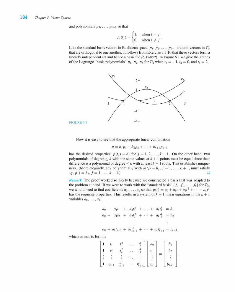
184 Chapter 3 Vector Spaces
and polynomials p3, . . . , pk+1 so that
pi(tj ) ={
1, when i = j
0, when i �= j.
Like the standard basis vectors in Euclidean space, p1, p2, . . . , pk+1 are unit vectors in Pkthat are orthogonal to one another. It follows from Exercise 3.3.10 that these vectors form alinearly independent set and hence a basis for Pk (why?). In Figure 6.1 we give the graphsof the Lagrange “basis polynomials” p1, p2, p3 for P2 when t1 = −1, t2 = 0, and t3 = 2.
FIGURE 6.1
–2 –1 2 3
–2
–1
1
2
p1p3
p2
Now it is easy to see that the appropriate linear combination
p = b1p1 + b2p2 + · · · + bk+1pk+1
has the desired properties: p(tj ) = bj for j = 1, 2, . . . , k + 1. On the other hand, twopolynomials of degree ≤ k with the same values at k + 1 points must be equal since theirdifference is a polynomial of degree ≤ k with at least k + 1 roots. This establishes unique-ness. (More elegantly, any polynomial q with q(tj ) = bj , j = 1, . . . , k + 1, must satisfy〈q, pj 〉 = bj , j = 1, . . . , k + 1.)
Remark. The proof worked so nicely because we constructed a basis that was adapted tothe problem at hand. If we were to work with the “standard basis” {f0, f1, . . . , fk} for Pk ,we would need to find coefficients a0, . . . , ak so that p(t) = a0 + a1t + a2t
2 + · · · + aktkhas the requisite properties. This results in a system of k + 1 linear equations in the k + 1variables a0, . . . , ak:
a0 + a1t1 + a2t21 + · · · + akt
k1 = b1
a0 + a1t2 + a2t22 + · · · + akt
k2 = b2
...
a0 + a1tk+1 + a2t2k+1 + · · · + akt
kk+1 = bk+1,
which in matrix form is⎡⎢⎢⎢⎢⎢⎣
1 t1 t21 . . . t k1
1 t2 t22 . . . t k2...
......
. . ....
1 tk+1 t2k+1 . . . t kk+1
⎤⎥⎥⎥⎥⎥⎦
⎡⎢⎢⎢⎢⎢⎣
a0
a1
...
ak
⎤⎥⎥⎥⎥⎥⎦
=
⎡⎢⎢⎢⎢⎢⎣
b1
b2
...
bk+1
⎤⎥⎥⎥⎥⎥⎦.
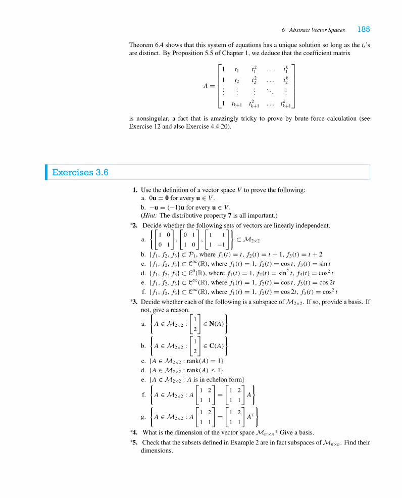
6 Abstract Vector Spaces 185
Theorem 6.4 shows that this system of equations has a unique solution so long as the ti’sare distinct. By Proposition 5.5 of Chapter 1, we deduce that the coefficient matrix
A =
⎡⎢⎢⎢⎢⎢⎣
1 t1 t21 . . . tk1
1 t2 t22 . . . tk2...
......
. . ....
1 tk+1 t2k+1 . . . t kk+1
⎤⎥⎥⎥⎥⎥⎦
is nonsingular, a fact that is amazingly tricky to prove by brute-force calculation (seeExercise 12 and also Exercise 4.4.20).
Exercises 3.6
1. Use the definition of a vector space V to prove the following:a. 0u = 0 for every u ∈ V .
b. −u = (−1)u for every u ∈ V .(Hint: The distributive property 7 is all important.)
2.∗ Decide whether the following sets of vectors are linearly independent.
a.
{[1 0
0 1
],
[0 1
1 0
],
[1 1
1 −1
]}⊂ M2×2
b. {f1, f2, f3} ⊂ P1, where f1(t) = t , f2(t) = t + 1, f3(t) = t + 2
c. {f1, f2, f3} ⊂ C∞(R), where f1(t) = 1, f2(t) = cos t , f3(t) = sin t
d. {f1, f2, f3} ⊂ C0(R), where f1(t) = 1, f2(t) = sin2 t , f3(t) = cos2 t
e. {f1, f2, f3} ⊂ C∞(R), where f1(t) = 1, f2(t) = cos t , f3(t) = cos 2t
f. {f1, f2, f3} ⊂ C∞(R), where f1(t) = 1, f2(t) = cos 2t , f3(t) = cos2 t
3.∗ Decide whether each of the following is a subspace of M2×2. If so, provide a basis. Ifnot, give a reason.
a.
{A ∈ M2×2 :
[1
2
]∈ N(A)
}
b.
{A ∈ M2×2 :
[1
2
]∈ C(A)
}
c. {A ∈ M2×2 : rank(A) = 1}d. {A ∈ M2×2 : rank(A) ≤ 1}e. {A ∈ M2×2 : A is in echelon form}f.
{A ∈ M2×2 : A
[1 2
1 1
]=[
1 2
1 1
]A
}
g.
{A ∈ M2×2 : A
[1 2
1 1
]=[
1 2
1 1
]AT
}
4.∗ What is the dimension of the vector space Mm×n? Give a basis.
5.∗ Check that the subsets defined in Example 2 are in fact subspaces of Mn×n. Find theirdimensions.
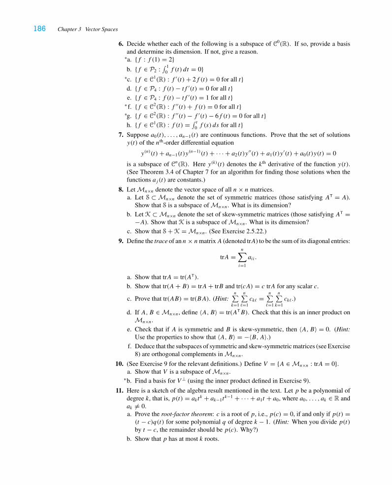
186 Chapter 3 Vector Spaces
6. Decide whether each of the following is a subspace of C0(R). If so, provide a basisand determine its dimension. If not, give a reason.a.∗ {f : f (1) = 2}b. {f ∈ P2 : ∫ 1
0 f (t) dt = 0}c.∗ {f ∈ C1(R) : f ′(t)+ 2f (t) = 0 for all t}d. {f ∈ P4 : f (t)− tf ′(t) = 0 for all t}e. {f ∈ P4 : f (t)− tf ′(t) = 1 for all t}f.∗ {f ∈ C2(R) : f ′′(t)+ f (t) = 0 for all t}g.∗ {f ∈ C2(R) : f ′′(t)− f ′(t)− 6f (t) = 0 for all t}h. {f ∈ C1(R) : f (t) = ∫ t
0 f (s) ds for all t}7. Suppose a0(t), . . . , an−1(t) are continuous functions. Prove that the set of solutionsy(t) of the nth-order differential equation
y(n)(t)+ an−1(t)y(n−1)(t)+ · · · + a2(t)y
′′(t)+ a1(t)y′(t)+ a0(t)y(t) = 0
is a subspace of Cn(R). Here y(k)(t) denotes the kth derivative of the function y(t).(See Theorem 3.4 of Chapter 7 for an algorithm for finding those solutions when thefunctions aj (t) are constants.)
8. Let Mn×n denote the vector space of all n× n matrices.a. Let S ⊂ Mn×n denote the set of symmetric matrices (those satisfying AT = A).
Show that S is a subspace of Mn×n. What is its dimension?
b. Let K ⊂ Mn×n denote the set of skew-symmetric matrices (those satisfying AT =−A). Show that K is a subspace of Mn×n. What is its dimension?
c. Show that S + K = Mn×n. (See Exercise 2.5.22.)
9. Define the trace of an n× nmatrixA (denoted trA) to be the sum of its diagonal entries:
trA =n∑i=1
aii .
a. Show that trA = tr(AT).
b. Show that tr(A+ B) = trA+ trB and tr(cA) = c trA for any scalar c.
c. Prove that tr(AB) = tr(BA). (Hint:n∑k=1
n∑�=1ck� =
n∑�=1
n∑k=1ck�.)
d. If A,B ∈ Mn×n, define 〈A,B〉 = tr(ATB). Check that this is an inner product onMn×n.
e. Check that if A is symmetric and B is skew-symmetric, then 〈A,B〉 = 0. (Hint:Use the properties to show that 〈A,B〉 = −〈B,A〉.)
f. Deduce that the subspaces of symmetric and skew-symmetric matrices (see Exercise8) are orthogonal complements in Mn×n.
10. (See Exercise 9 for the relevant definitions.) Define V = {A ∈ Mn×n : trA = 0}.a. Show that V is a subspace of Mn×n.b.∗ Find a basis for V ⊥ (using the inner product defined in Exercise 9).
11. Here is a sketch of the algebra result mentioned in the text. Let p be a polynomial ofdegree k, that is, p(t) = akt
k + ak−1tk−1 + · · · + a1t + a0, where a0, . . . , ak ∈ R and
ak �= 0.a. Prove the root-factor theorem: c is a root of p, i.e., p(c) = 0, if and only if p(t) =(t − c)q(t) for some polynomial q of degree k − 1. (Hint: When you divide p(t)by t − c, the remainder should be p(c). Why?)
b. Show that p has at most k roots.
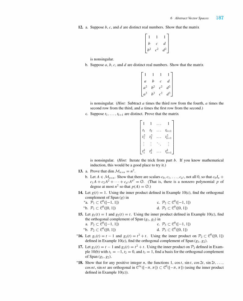
6 Abstract Vector Spaces 187
12. a. Suppose b, c, and d are distinct real numbers. Show that the matrix⎡⎢⎢⎣
1 1 1
b c d
b2 c2 d2
⎤⎥⎥⎦
is nonsingular.
b. Suppose a, b, c, and d are distinct real numbers. Show that the matrix
⎡⎢⎢⎢⎢⎣
1 1 1 1
a b c d
a2 b2 c2 d2
a3 b3 c3 d3
⎤⎥⎥⎥⎥⎦
is nonsingular. (Hint: Subtract a times the third row from the fourth, a times thesecond row from the third, and a times the first row from the second.)
c. Suppose t1, . . . , tk+1 are distinct. Prove that the matrix⎡⎢⎢⎢⎢⎢⎢⎢⎢⎣
1 1 . . . 1
t1 t2 . . . tk+1
t21 t22 . . . t2k+1...
.... . .
...
t k1 tk2 . . . t kk+1
⎤⎥⎥⎥⎥⎥⎥⎥⎥⎦
is nonsingular. (Hint: Iterate the trick from part b. If you know mathematicalinduction, this would be a good place to try it.)
13. a. Prove that dim Mn×n = n2.
b. Let A ∈ Mn×n. Show that there are scalars c0, c1, . . . , cn2 , not all 0, so that c0In +c1A+ c2A
2 + · · · + cn2An2 = O. (That is, there is a nonzero polynomial p of
degree at most n2 so that p(A) = O.)
14. Let g(t) = 1. Using the inner product defined in Example 10(c), find the orthogonalcomplement of Span (g) ina.∗ P1 ⊂ C0([−1, 1])b.∗ P1 ⊂ C0([0, 1])
c. P2 ⊂ C0([−1, 1])d. P2 ⊂ C0([0, 1])
15. Let g1(t) = 1 and g2(t) = t . Using the inner product defined in Example 10(c), findthe orthogonal complement of Span (g1, g2) ina. P2 ⊂ C0([−1, 1])b.∗ P2 ⊂ C0([0, 1])
c. P3 ⊂ C0([−1, 1])d. P3 ⊂ C0([0, 1])
16.∗ Let g1(t) = t − 1 and g2(t) = t2 + t . Using the inner product on P2 ⊂ C0([0, 1])defined in Example 10(c), find the orthogonal complement of Span (g1, g2).
17. Let g1(t) = t − 1 and g2(t) = t2 + t . Using the inner product on P2 defined in Exam-ple 10(b) with t1 = −1, t2 = 0, and t3 = 1, find a basis for the orthogonal complementof Span (g1, g2).
18.∗ Show that for any positive integer n, the functions 1, cos t , sin t , cos 2t , sin 2t, . . . ,cos nt , sin nt are orthogonal in C∞([−π, π ]) ⊂ C0([−π, π ]) (using the inner productdefined in Example 10(c)).
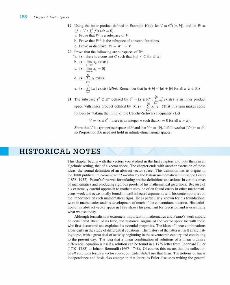
188 Chapter 3 Vector Spaces
19. Using the inner product defined in Example 10(c), let V = C0([a, b]), and let W ={f ∈ V : ∫ b
af (t) dt = 0}.
a. Prove thatW is a subspace of V .
b. Prove thatW⊥ is the subspace of constant functions.
c. Prove or disprove: W +W⊥ = V .
20. Prove that the following are subspaces of Rω.a.∗ {x : there is a constant C such that |xk| ≤ C for all k}b. {x : lim
k→∞ xk exists}c. {x : lim
k→∞ xk = 0}
d. {x :∞∑k=1xk exists}
e. {x :∞∑k=1
|xk| exists} (Hint: Remember that |a + b| ≤ |a| + |b| for all a, b ∈ R.)
21. The subspace �2 ⊂ Rω defined by �2 = {x ∈ Rω :∞∑k=1x2k exists} is an inner product
space with inner product defined by 〈x, y〉 =∞∑k=1xkyk . (That this sum makes sense
follows by “taking the limit” of the Cauchy-Schwarz Inequality.) Let
V = {x ∈ �2 : there is an integer n such that xk = 0 for all k > n}.Show thatV is a (proper) subspace of �2 and thatV ⊥ = {0}. It follows that (V ⊥)⊥ = �2,so Proposition 3.6 need not hold in infinite-dimensional spaces.
HISTORICAL NOTESThis chapter begins with the vectors you studied in the first chapters and puts them in analgebraic setting, that of a vector space. The chapter ends with another extension of theseideas, the formal definition of an abstract vector space. This definition has its origins inthe 1888 publication Geometrical Calculus by the Italian mathematician Giuseppe Peano(1858–1932). Peano’s forte was formulating precise definitions and axioms in various areasof mathematics and producing rigorous proofs of his mathematical assertions. Because ofhis extremely careful approach to mathematics, he often found errors in other mathemati-cians’work and occasionally found himself in heated arguments with his contemporaries onthe importance of such mathematical rigor. He is particularly known for his foundationalwork in mathematics and his development of much of the concomitant notation. His defini-tion of an abstract vector space in 1888 shows his penchant for precision and is essentiallywhat we use today.
Although formalism is extremely important in mathematics and Peano’s work shouldbe considered ahead of its time, the historical origins of the vector space lie with thosewho first discovered and exploited its essential properties. The ideas of linear combinationsarose early in the study of differential equations. The history of the latter is itself a fascinat-ing topic, with a great deal of activity beginning in the seventeenth century and continuingto the present day. The idea that a linear combination of solutions of a linear ordinarydifferential equation is itself a solution can be found in a 1739 letter from Leonhard Euler(1707–1783) to Johann Bernoulli (1667–1748). Of course, this means that the collectionof all solutions forms a vector space, but Euler didn’t use that term. The notions of linearindependence and basis also emerge in that letter, as Euler discusses writing the general

Historical Notes 189
solution of the differential equation as a linear combination of certain base solutions. Theseideas continued to show up in works of other great mathematicians who studied differen-tial equations, notably Jean le Rond d’Alembert (1717–1783) and Joseph-Louis Lagrange(1736–1813). Not long thereafter, the ideas of vector space and dimension found their wayinto the study of geometry with the work of Hermann Gunther Grassmann (1809–1877).In 1844 he published a seminal work describing his “calculus of extension,” now calledexterior algebra. Because so many people found his work unreadable, he ultimately revisedit and published Die Ausdehnungslehre in 1862. The objects he introduced are linear com-binations of symbols representing points, lines, and planes in various dimensions. In fact,it was Grassmann’s work that inspired Peano to make the modern definitions of basis anddimensions.
The history of dimension is itself a fascinating subject. For vector spaces, we haveseen that the definition is fairly intuitive. On the other hand, there are some very interestingparadoxes that arise when one examines the notion of dimension more carefully. In 1877Georg Cantor (1845–1918) made an amazing and troubling discovery: He proved that thatthere is a one-to-one correspondence between points of R and points of R2. Althoughintuitively the (two-dimensional) plane is bigger than the (one-dimensional) line, Cantor’sargument says that they each have the same “number” of points.
Of course, the one-to-one correspondence described by Cantor must not be a very nicefunction, so one might consider Cantor’s result not as a problem with the concept of di-mension but as evidence that perhaps functions can be badly behaved. However, in 1890Peano further confounded the situation by producing a continuous function from the lineinto the plane that touches every point of a square. The actual definition of dimensionthat finally came about to resolve these issues is too involved for us to discuss here, as itentails elements of the branch of mathematics known as topology and objects called mani-folds. The key players in this work were Georg Friedrich Bernhard Riemann (1826–1866),J. Henri Poincaré (1854–1912), and L. E. J. Brouwer (1881–1966).
Even today, new discoveries and definitions shatter people’s expectations of dimension.Cantor and Peano did not realize that they were laying the groundwork for what is nowthe study of fractals or fractal geometry. Benoît Mandelbrot (1924–) coined the termfractal (from the Latin fractus, describing the appearance of a broken stone as irregularand fragmented) and launched a fascinating area of study. Fractal curves are strange beastsin that they always appear the same no matter how closely you look at them. When thenotions of dimension were extended to capture this behavior, mathematicians had discoveredgeometric figures with fractional dimension. Indeed, the coastline of Britain could actuallybe considered to have fractal dimension approximately 1.2. The study of fractals is a veryactive field of research today.

This page intentionally left blank
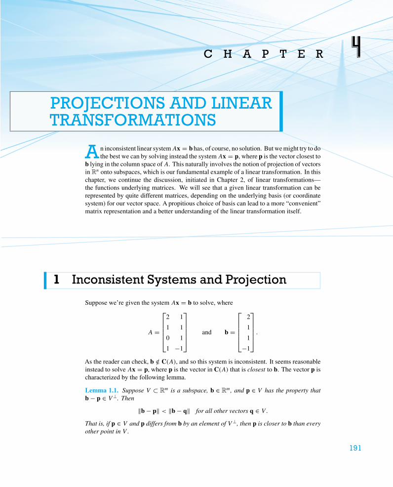
191
C H A P T E R 4PROJECTIONS AND LINEARTRANSFORMATIONS
A n inconsistent linear systemAx = b has, of course, no solution. But we might try to dothe best we can by solving instead the systemAx = p, where p is the vector closest to
b lying in the column space ofA. This naturally involves the notion of projection of vectorsin Rn onto subspaces, which is our fundamental example of a linear transformation. In thischapter, we continue the discussion, initiated in Chapter 2, of linear transformations—the functions underlying matrices. We will see that a given linear transformation can berepresented by quite different matrices, depending on the underlying basis (or coordinatesystem) for our vector space. A propitious choice of basis can lead to a more “convenient”matrix representation and a better understanding of the linear transformation itself.
1 Inconsistent Systems and Projection
Suppose we’re given the system Ax = b to solve, where
A =
⎡⎢⎢⎢⎢⎣
2 1
1 1
0 1
1 −1
⎤⎥⎥⎥⎥⎦
and b =
⎡⎢⎢⎢⎢⎣
2
1
1
−1
⎤⎥⎥⎥⎥⎦.
As the reader can check, b /∈ C(A), and so this system is inconsistent. It seems reasonableinstead to solve Ax = p, where p is the vector in C(A) that is closest to b. The vector p ischaracterized by the following lemma.
Lemma 1.1. Suppose V ⊂ Rm is a subspace, b ∈ Rm, and p ∈ V has the property thatb − p ∈ V ⊥. Then
‖b − p‖ < ‖b − q‖ for all other vectors q ∈ V.That is, if p ∈ V and p differs from b by an element of V ⊥, then p is closer to b than everyother point in V .
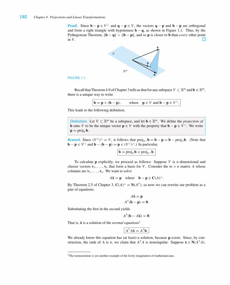
192 Chapter 4 Projections and Linear Transformations
Proof. Since b − p ∈ V ⊥ and q − p ∈ V , the vectors q − p and b − p are orthogonaland form a right triangle with hypotenuse b − q, as shown in Figure 1.1. Thus, by thePythagorean Theorem, ‖b − q‖ > ‖b − p‖, and so p is closer to b than every other pointin V .
FIGURE 1.1
b
V
p
qRm
Recall that Theorem 4.9 of Chapter 3 tells us that for any subspaceV ⊂ Rm and b ∈ Rm,there is a unique way to write
b = p + (b − p), where p ∈ V and b − p ∈ V ⊥.
This leads to the following definition.
Definition. Let V ⊂ Rm be a subspace, and let b ∈ Rm. We define the projection ofb onto V to be the unique vector p ∈ V with the property that b − p ∈ V ⊥. We writep = projV b.
Remark. Since (V ⊥)⊥ = V , it follows that projV ⊥b = b − p = b − projV b. (Note thatb − p ∈ V ⊥ and b − (b − p) = p ∈ (V ⊥)⊥.) In particular,
b = projV b + projV ⊥b.
To calculate p explicitly, we proceed as follows: Suppose V is n-dimensional andchoose vectors v1, . . . , vn that form a basis for V . Consider the m× n matrix A whosecolumns are v1, . . . , vn. We want to solve
Ax = p where b − p ∈ C(A)⊥.
By Theorem 2.5 of Chapter 3, C(A)⊥ = N(AT), so now we can rewrite our problem as apair of equations:
Ax = p
AT(b − p) = 0.
Substituting the first in the second yields
AT(b − Ax) = 0.
That is, x is a solution of the normal equations1
ATAx = ATb.
We already know this equation has (at least) a solution, because p exists. Since, by con-struction, the rank of A is n, we claim that ATA is nonsingular: Suppose x ∈ N(ATA).
1The nomenclature is yet another example of the lively imagination of mathematicians.
1 Inconsistent Systems and Projection 193
This means
(ATA)x = AT(Ax) = 0,
so, dotting with x, we get
AT(Ax) · x = Ax · Ax = ‖Ax‖2 = 0;thereforeAx = 0, and sinceA has rank n, we conclude that x = 0. As a result, we have thefollowing definition.
Definition. Given anm× nmatrixA of rankn, the least squares solution of the equationAx = b is the unique solution2 of the normal equations
(ATA)x = ATb.
Remark. When rank(A) < n, the normal equations are still consistent (see Exercise 3.4.24)but have infinitely many solutions. Every one of those solutions x gives rise to the sameprojection Ax = p, because p is the unique vector in C(A) with the property that b − p ∈N(AT). But we define the least squares solution to be the unique vector x ∈ R(A) thatsatisfies the normal equations; of all the solutions, this is the one of least length. (SeeProposition 4.10 of Chapter 3.) This leads to the pseudoinverse that is important in numer-ical analysis. See Strang’s books for more details.
Summarizing, we have proved the following proposition.
Proposition 1.2. Suppose V ⊂ Rm is an n-dimensional subspace with basis vectorsv1, . . . , vn, and let A be the m× n matrix whose columns are these basis vectors. Given avector b ∈ Rm, the projection of b onto V is obtained by multiplying the unique solution ofthe normal equations (ATA)x = ATb by the matrix A. That is,
p = projV b = Ax = (A(ATA)−1AT)b.
EXAMPLE 1
To solve the problem we posed at the beginning of the section, we wish to find the leastsquares solution of the system Ax = b, where
A =
⎡⎢⎢⎢⎢⎣
2 1
1 1
0 1
1 −1
⎤⎥⎥⎥⎥⎦
and b =
⎡⎢⎢⎢⎢⎣
2
1
1
−1
⎤⎥⎥⎥⎥⎦.
We need only solve the normal equations ATAx = ATb. Now,
ATA =[
6 2
2 4
]and ATb =
[4
5
],
2x is called the least squares solution because it minimizes the sum of squares ‖b − q‖2 = (b1 − q1)2 + · · · +
(bm − qm)2, among all vectors q = Ax for some x ∈ Rn.
194 Chapter 4 Projections and Linear Transformations
and so, using the formula for the inverse of a 2 × 2 matrix in Example 4 on p. 105, we findthat
x = (ATA)−1ATb = 1
20
[4 −2
−2 6
][4
5
]= 1
10
[3
11
]
is the least squares solution. Moreover, while we’re at it, we can find the projection of bonto C(A) by calculating
Ax =
⎡⎢⎢⎢⎢⎣
2 1
1 1
0 1
1 −1
⎤⎥⎥⎥⎥⎦
(1
10
[3
11
])= 1
10
⎡⎢⎢⎢⎢⎣
17
14
11
−8
⎤⎥⎥⎥⎥⎦.
We note next that Proposition 1.2 gives us an explicit formula for projection onto asubspace V ⊂ Rm, generalizing the case of dim V = 1 given in Chapter 1. Since we have
p = projV b = (A(ATA)−1AT)b
for every vector b ∈ Rm, it follows that the matrix
(∗) PV = A(ATA)−1AT
is the appropriate “projection matrix”; that is,
projV = μPV = μA(ATA)−1AT .
Remark. It can be rather messy to compute PV , since along the way we must calculate(ATA)−1. Later in this chapter, we will see that a clever choice of basis will make thiscalculation much easier.
Remark. Since we have written projV = μPV for the projection matrix PV , it follows thatprojV is a linear transformation. (We already checked this for one-dimensional subspacesV in Chapter 2.) In Exercise 13 we ask the reader to show this directly, using the definitionon p. 192.
EXAMPLE 2
If b ∈ C(A) to begin with, then b = Ax for some x ∈ Rn, and
PV b = (A(ATA)−1AT)b = A(ATA)−1(ATA)x = Ax = b,
as it should be. And if b ∈ C(A)⊥, then b ∈ N(AT), so
PV b = (A(ATA)−1AT)b = A(ATA)−1(ATb) = 0,
as it should be.
EXAMPLE 3
Note that when dim V = 1, we recover our formula for projection onto a line from Section2 of Chapter 1. If a ∈ V ⊂ Rm is a nonzero vector, we consider it as an m× 1 matrix, andthe projection formula becomes
PV = 1
‖a‖2aaT;
1 Inconsistent Systems and Projection 195
that is,
PV b = 1
‖a‖2(aaT)b = 1
‖a‖2a(aTb) = a · b
‖a‖2a,
as before. For example, if
a =
⎡⎢⎢⎣
2
1
0
⎤⎥⎥⎦ , then PV = 1
5
⎡⎢⎢⎣
4 2 0
2 1 0
0 0 0
⎤⎥⎥⎦ .
(This might be a good time to review Example 3 in Section 5 of Chapter 2. For a ∈ Rm,remember that aaT is an m×m matrix, whereas aTa is a 1 × 1 matrix, i.e., a scalar.)
EXAMPLE 4
Let V ⊂ R3 be the plane defined by the equation x1 − 2x2 + x3 = 0. Then
v1 =
⎡⎢⎢⎣
2
1
0
⎤⎥⎥⎦ and v2 =
⎡⎢⎢⎣
−1
0
1
⎤⎥⎥⎦
form a basis for V , and we take
A =
⎡⎢⎢⎣
2 −1
1 0
0 1
⎤⎥⎥⎦ .
Then, since
ATA =[
5 −2
−2 2
], we have (ATA)−1 = 1
6
[2 2
2 5
],
and so
PV = A(ATA)−1AT = 1
6
⎡⎢⎢⎣
2 −1
1 0
0 1
⎤⎥⎥⎦[
2 2
2 5
][2 1 0
−1 0 1
]= 1
6
⎡⎢⎢⎣
5 2 −1
2 2 2
−1 2 5
⎤⎥⎥⎦ .
Here is an alternative solution. We have already seen that
projV b = b − proj(V ⊥)b.
In matrix notation, this can be rewritten as
PV = I3 − PV ⊥ .
Since V ⊥ is spanned by a normal vector, a, to the plane, as in Example 3, we have
PV ⊥ = 1
‖a‖2aaT, and so PV = I3 − 1
‖a‖2aaT.
196 Chapter 4 Projections and Linear Transformations
In our case, we have a =⎡⎢⎣
1
−2
1
⎤⎥⎦, and so
I3 − 1
‖a‖2(aaT) =
⎡⎢⎢⎣
1 0 0
0 1 0
0 0 1
⎤⎥⎥⎦− 1
6
⎡⎢⎢⎣
1
−2
1
⎤⎥⎥⎦[1 −2 1
]
=
⎡⎢⎢⎣
1 0 0
0 1 0
0 0 1
⎤⎥⎥⎦− 1
6
⎡⎢⎢⎣
1 −2 1
−2 4 −2
1 −2 1
⎤⎥⎥⎦ = 1
6
⎡⎢⎢⎣
5 2 −1
2 2 2
−1 2 5
⎤⎥⎥⎦ ,
just as before. This is a useful trick to keep in mind. It is sometimes easier to calculate PV ⊥
than PV ; generally, it is easier to project onto the subspace that has the smaller dimension.
In the next section, we’ll see the geometry underlying the formula for the projectionmatrix.
1.1 Data FittingPerhaps the most natural setting in which inconsistent systems of linear equations arise isthat of fitting data to a linear model when they won’t quite fit. The least squares solutionof such linear problems is called the least squares line fitting the points (or the line ofregression in statistics). Even nonlinear problems can sometimes be rephrased linearly.For example, fitting a parabola y = ax2 + bx + c to data points in the xy-plane, as we sawin Section 6 of Chapter 1, is still a matter of solving a system of linear equations. Even moresurprisingly, in our laboratory work many of us have tried to find the right constants a and kso that the data points (x1, y1), . . . , (xm, ym) lie on the curve y = axk . Taking logarithms,we see that this is equivalent to fitting the points (ui, vi) = (ln xi, ln yi), i = 1, . . . , m, toa line v = ku+ ln a.3
EXAMPLE 5
Find the least squares line y = ax + b for the data points (−1, 0), (1, 1), and (2, 3). (SeeFigure 1.2.) We get the system of equations
−1a + b = 0
1a + b = 1
2a + b = 3 ,
which in matrix form becomes
A
[a
b
]=
⎡⎢⎢⎣
−1 1
1 1
2 1
⎤⎥⎥⎦[a
b
]=
⎡⎢⎢⎣
0
1
3
⎤⎥⎥⎦ .
3This is why “log-log paper” was so useful before the advent of calculators and computers.
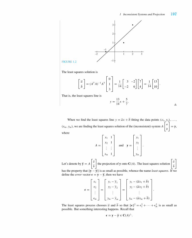
1 Inconsistent Systems and Projection 197
FIGURE 1.2
–2
–1
1 2 3
–1
1
2
3
The least squares solution is
[a
b
]= (ATA)−1AT
⎡⎢⎢⎣
0
1
3
⎤⎥⎥⎦ = 1
14
[3 −2
−2 6
][7
4
]= 1
14
[13
10
].
That is, the least squares line is
y = 13
14x + 5
7.
When we find the least squares line y = ax + b fitting the data points (x1, y1), . . . ,
(xm, ym), we are finding the least squares solution of the (inconsistent) systemA
[a
b
]= y,
where
A =
⎡⎢⎢⎢⎢⎢⎣
x1 1
x2 1...
...
xm 1
⎤⎥⎥⎥⎥⎥⎦
and y =
⎡⎢⎢⎢⎢⎢⎣
y1
y2
...
ym
⎤⎥⎥⎥⎥⎥⎦.
Let’s denote by y = A
[a
b
]the projection of y onto C(A). The least squares solution
[a
b
]
has the property that ‖y − y‖ is as small as possible, whence the name least squares. If wedefine the error vector ε = y − y, then we have
ε =
⎡⎢⎢⎢⎢⎢⎣
ε1
ε2
...
εm
⎤⎥⎥⎥⎥⎥⎦
=
⎡⎢⎢⎢⎢⎢⎣
y1 − y1
y2 − y2...
ym − ym
⎤⎥⎥⎥⎥⎥⎦
=
⎡⎢⎢⎢⎢⎢⎣
y1 − (ax1 + b)y2 − (ax2 + b)
...
ym − (axm + b)
⎤⎥⎥⎥⎥⎥⎦.
The least squares process chooses a and b so that ‖ε‖2 = ε21 + · · · + ε2
m is as small aspossible. But something interesting happens. Recall that
ε = y − y ∈ C(A)⊥.
198 Chapter 4 Projections and Linear Transformations
Thus, ε is orthogonal to each of the column vectors of A, and so, in particular,
⎡⎢⎢⎣ε1
...
εm
⎤⎥⎥⎦ ·
⎡⎢⎢⎣
1...
1
⎤⎥⎥⎦ = ε1 + · · · + εm = 0.
That is, in the process of minimizing the sum of the squares of the errors εi , we have in factmade their (algebraic) sum equal to 0.
Exercises 4.1
1. By first finding the projection onto V ⊥, find the projection of the given vector b ∈ Rm
onto the given hyperplane V ⊂ Rm.a. V = {x1 + x2 + x3 = 0} ⊂ R3, b = (2, 1, 1)
b.∗ V = {x1 + x2 + x3 = 0} ⊂ R4, b = (0, 1, 2, 3)
c. V = {x1 − x2 + x3 + 2x4 = 0} ⊂ R4, b = (1, 1, 1, 1)
2. Use the formula PV = A(ATA)−1AT for the projection matrix to check that PV = P TV
and P 2V = PV . Show that I − PV has the same properties, and explain why.
3.∗ Let V = Span((1, 1,−1), (−2, 0, 1)
) ⊂ R3. Construct the matrix PV representingprojVa. by finding PV ⊥ ;
b. by using the formula (∗) on p. 194.
4. LetV = Span((1, 0, 1), (0, 1,−2)
) ⊂ R3. Construct the matrixPV representing projVa. by finding PV ⊥ ;
b. by using the formula (∗) on p. 194.
5. Let V = Span((1, 0, 1, 0), (0, 1, 0, 1), (1, 1,−1,−1)
) ⊂ R4. Construct the matrixPV representing projVa. by finding PV ⊥ ;
b. by using the formula (∗) on p. 194.
6.∗ Find the least squares solution of
x1 + x2 = 4
2x1 + x2 = −2
x1 − x2 = 1 .
Use your answer to find the point on the plane spanned by (1, 2, 1) and (1, 1,−1) thatis closest to (4,−2, 1).
7. Find the least squares solution of
x1 + x2 = 1
x1 − 3x2 = 4
2x1 + x2 = 3 .
Use your answer to find the point on the plane spanned by (1, 1, 2) and (1,−3, 1) thatis closest to (1, 4, 3).
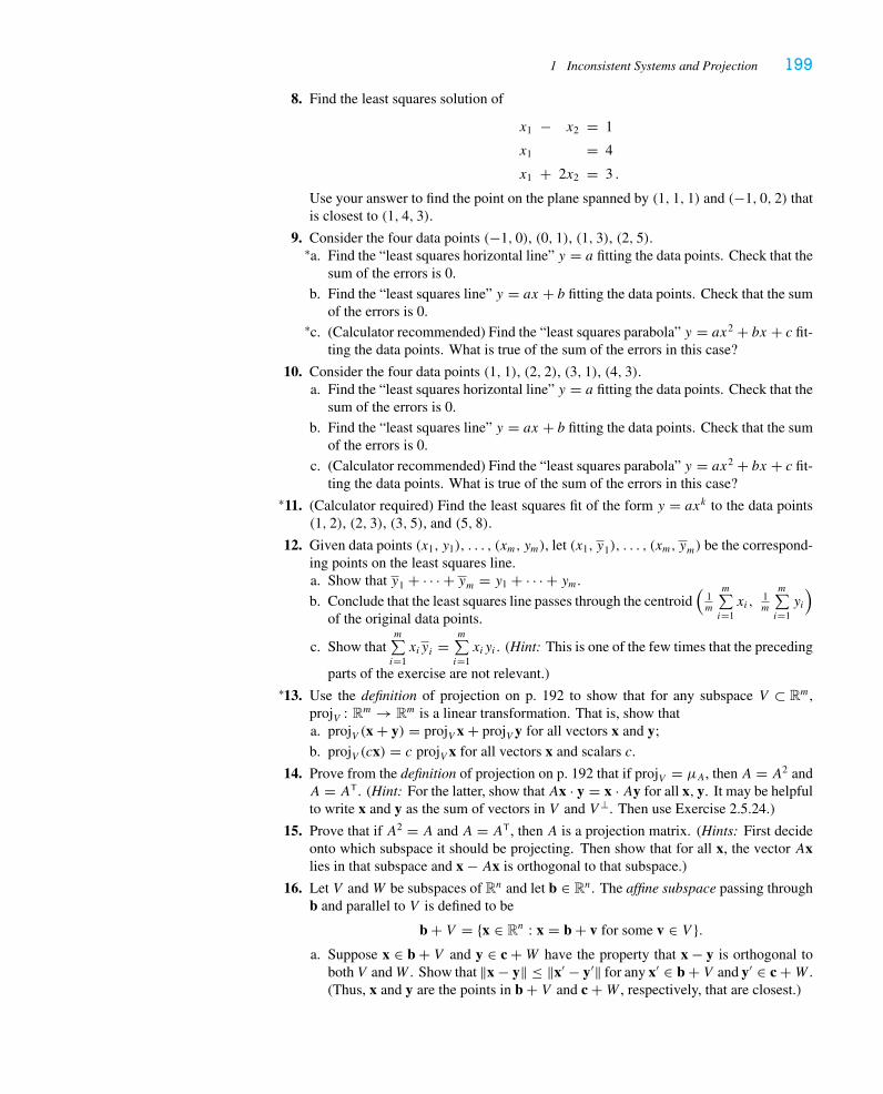
1 Inconsistent Systems and Projection 199
8. Find the least squares solution of
x1 − x2 = 1
x1 = 4
x1 + 2x2 = 3 .
Use your answer to find the point on the plane spanned by (1, 1, 1) and (−1, 0, 2) thatis closest to (1, 4, 3).
9. Consider the four data points (−1, 0), (0, 1), (1, 3), (2, 5).a.∗ Find the “least squares horizontal line” y = a fitting the data points. Check that the
sum of the errors is 0.
b. Find the “least squares line” y = ax + b fitting the data points. Check that the sumof the errors is 0.
c.∗ (Calculator recommended) Find the “least squares parabola” y = ax2 + bx + c fit-ting the data points. What is true of the sum of the errors in this case?
10. Consider the four data points (1, 1), (2, 2), (3, 1), (4, 3).a. Find the “least squares horizontal line” y = a fitting the data points. Check that the
sum of the errors is 0.
b. Find the “least squares line” y = ax + b fitting the data points. Check that the sumof the errors is 0.
c. (Calculator recommended) Find the “least squares parabola” y = ax2 + bx + c fit-ting the data points. What is true of the sum of the errors in this case?
11.∗ (Calculator required) Find the least squares fit of the form y = axk to the data points(1, 2), (2, 3), (3, 5), and (5, 8).
12. Given data points (x1, y1), . . . , (xm, ym), let (x1, y1), . . . , (xm, ym) be the correspond-ing points on the least squares line.a. Show that y1 + · · · + ym = y1 + · · · + ym.
b. Conclude that the least squares line passes through the centroid(
1m
m∑i=1xi,
1m
m∑i=1yi
)
of the original data points.
c. Show thatm∑i=1xiyi =
m∑i=1xiyi . (Hint: This is one of the few times that the preceding
parts of the exercise are not relevant.)
13.∗ Use the definition of projection on p. 192 to show that for any subspace V ⊂ Rm,projV : Rm → Rm is a linear transformation. That is, show thata. projV (x + y) = projV x + projV y for all vectors x and y;
b. projV (cx) = c projV x for all vectors x and scalars c.
14. Prove from the definition of projection on p. 192 that if projV = μA, then A = A2 andA = AT. (Hint: For the latter, show thatAx · y = x · Ay for all x, y. It may be helpfulto write x and y as the sum of vectors in V and V ⊥. Then use Exercise 2.5.24.)
15. Prove that if A2 = A and A = AT, then A is a projection matrix. (Hints: First decideonto which subspace it should be projecting. Then show that for all x, the vector Axlies in that subspace and x − Ax is orthogonal to that subspace.)
16. Let V andW be subspaces of Rn and let b ∈ Rn. The affine subspace passing throughb and parallel to V is defined to be
b + V = {x ∈ Rn : x = b + v for some v ∈ V }.a. Suppose x ∈ b + V and y ∈ c +W have the property that x − y is orthogonal to
both V andW . Show that ‖x − y‖ ≤ ‖x′ − y′‖ for any x′ ∈ b + V and y′ ∈ c +W .(Thus, x and y are the points in b + V and c +W , respectively, that are closest.)
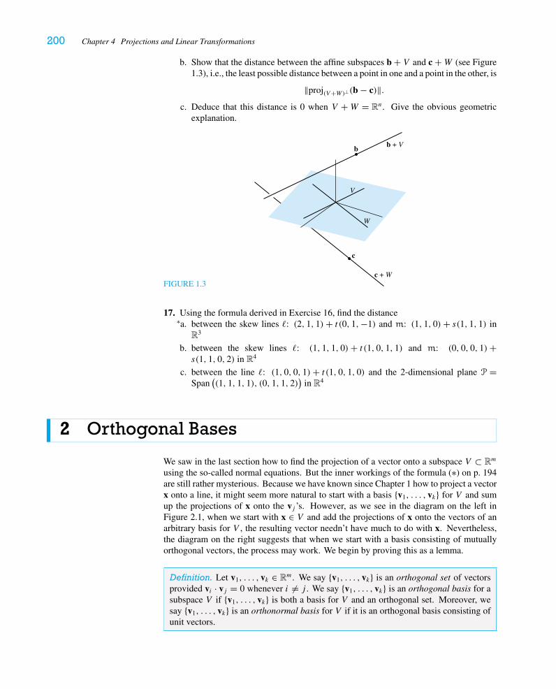
200 Chapter 4 Projections and Linear Transformations
b. Show that the distance between the affine subspaces b + V and c +W (see Figure1.3), i.e., the least possible distance between a point in one and a point in the other, is
‖proj(V+W)⊥(b − c)‖.c. Deduce that this distance is 0 when V +W = Rn. Give the obvious geometric
explanation.
FIGURE 1.3c + W
c
b + Vb
V
W
17. Using the formula derived in Exercise 16, find the distancea.∗ between the skew lines �: (2, 1, 1)+ t (0, 1,−1) and m: (1, 1, 0)+ s(1, 1, 1) in
R3
b. between the skew lines �: (1, 1, 1, 0)+ t (1, 0, 1, 1) and m: (0, 0, 0, 1)+s(1, 1, 0, 2) in R4
c. between the line �: (1, 0, 0, 1)+ t (1, 0, 1, 0) and the 2-dimensional plane P =Span
((1, 1, 1, 1), (0, 1, 1, 2)
)in R4
2 Orthogonal Bases
We saw in the last section how to find the projection of a vector onto a subspace V ⊂ Rm
using the so-called normal equations. But the inner workings of the formula (∗) on p. 194are still rather mysterious. Because we have known since Chapter 1 how to project a vectorx onto a line, it might seem more natural to start with a basis {v1, . . . , vk} for V and sumup the projections of x onto the vj ’s. However, as we see in the diagram on the left inFigure 2.1, when we start with x ∈ V and add the projections of x onto the vectors of anarbitrary basis for V , the resulting vector needn’t have much to do with x. Nevertheless,the diagram on the right suggests that when we start with a basis consisting of mutuallyorthogonal vectors, the process may work. We begin by proving this as a lemma.
Definition. Let v1, . . . , vk ∈ Rm. We say {v1, . . . , vk} is an orthogonal set of vectorsprovided vi · vj = 0 whenever i = j . We say {v1, . . . , vk} is an orthogonal basis for asubspace V if {v1, . . . , vk} is both a basis for V and an orthogonal set. Moreover, wesay {v1, . . . , vk} is an orthonormal basis for V if it is an orthogonal basis consisting ofunit vectors.
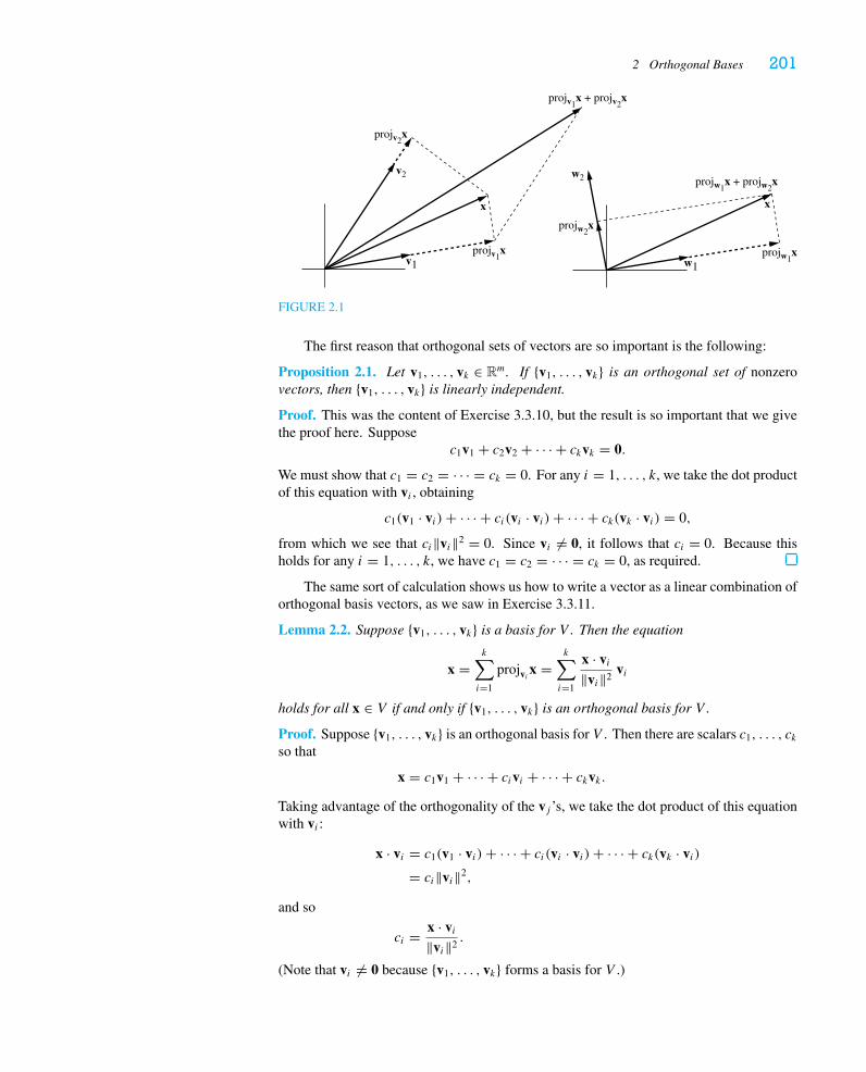
2 Orthogonal Bases 201
x x
projv2x
projw2x
projv1x projw1
x
projv1x + projv2
x
projw1x + projw2
xv2 w2
v1 w1
FIGURE 2.1
The first reason that orthogonal sets of vectors are so important is the following:
Proposition 2.1. Let v1, . . . , vk ∈ Rm. If {v1, . . . , vk} is an orthogonal set of nonzerovectors, then {v1, . . . , vk} is linearly independent.
Proof. This was the content of Exercise 3.3.10, but the result is so important that we givethe proof here. Suppose
c1v1 + c2v2 + · · · + ckvk = 0.
We must show that c1 = c2 = · · · = ck = 0. For any i = 1, . . . , k, we take the dot productof this equation with vi , obtaining
c1(v1 · vi )+ · · · + ci(vi · vi )+ · · · + ck(vk · vi ) = 0,
from which we see that ci‖vi‖2 = 0. Since vi = 0, it follows that ci = 0. Because thisholds for any i = 1, . . . , k, we have c1 = c2 = · · · = ck = 0, as required.
The same sort of calculation shows us how to write a vector as a linear combination oforthogonal basis vectors, as we saw in Exercise 3.3.11.
Lemma 2.2. Suppose {v1, . . . , vk} is a basis for V . Then the equation
x =k∑i=1
projvix =k∑i=1
x · vi‖vi‖2
vi
holds for all x ∈ V if and only if {v1, . . . , vk} is an orthogonal basis for V .
Proof. Suppose {v1, . . . , vk} is an orthogonal basis for V . Then there are scalars c1, . . . , ckso that
x = c1v1 + · · · + civi + · · · + ckvk.Taking advantage of the orthogonality of the vj ’s, we take the dot product of this equationwith vi :
x · vi = c1(v1 · vi )+ · · · + ci(vi · vi )+ · · · + ck(vk · vi )
= ci‖vi‖2,
and so
ci = x · vi‖vi‖2
.
(Note that vi = 0 because {v1, . . . , vk} forms a basis for V .)
202 Chapter 4 Projections and Linear Transformations
Conversely, suppose that every vector x ∈ V is the sum of its projections on v1, . . . , vk .Let’s just examine what this means when x = v1: We are given that
v1 =k∑i=1
projviv1 =k∑i=1
v1 · vi‖vi‖2
vi .
Recall from Proposition 3.1 of Chapter 3 that every vector has a unique expansion as alinear combination of basis vectors, so comparing coefficients of v2, . . . , vk on either sideof this equation, we conclude that
v1 · vi = 0 for all i = 2, . . . , k.
A similar argument shows that vi · vj = 0 for all i = j , and the proof is complete.
We recall that whenever {v1, . . . , vk} is a basis forV , every vector x ∈ V can be writtenuniquely as a linear combination
x = c1v1 + c2v2 + · · · + ckvk,where the coefficients c1, c2, . . . , ck are called the coordinates of x with respect to the basis{v1, . . . , vk}. We emphasize that, as in Lemma 2.2, when {v1, . . . , vk} forms an orthogonalbasis for V , the dot product gives the coordinates of x. As we shall see in Section 4, whenthe basis is not orthogonal, it is more tedious to compute these coordinates.
Not only do orthogonal bases make it easy to calculate coordinates, they also makeprojections quite easy to compute, as we now see.
Proposition 2.3. Let V ⊂ Rm be a k-dimensional subspace. The equation
(†) projV b =k∑i=1
projvib =k∑i=1
b · vi‖vi‖2
vi
holds for all b ∈ Rm if and only if {v1, . . . , vk} is an orthogonal basis for V .
Proof. Assume {v1, . . . , vk} is an orthogonal basis for V and let b ∈ Rm. Write b =p + (b − p), where p = projV b (and so b − p ∈ V ⊥). Then, since p ∈ V , it follows from
Lemma 2.2 that p =k∑i=1
p · vi‖vi‖2
vi . Moreover, for i = 1, . . . , k, we have b · vi = p · vi ,
since b − p ∈ V ⊥. Thus,
projV b = p =k∑i=1
projvip =k∑i=1
p · vi‖vi‖2
vi =k∑i=1
b · vi‖vi‖2
vi =k∑i=1
projvib.
Conversely, suppose projV b =k∑i=1
projvib for all b ∈ Rm. In particular, when b ∈ V , we
deduce that b = projV b can be written as a linear combination of v1, . . . , vk , so these vectorsspan V ; since V is k-dimensional, {v1, . . . , vk} gives a basis for V . By Lemma 2.2, it mustbe an orthogonal basis.
We now have another way to calculate the projection of a vector on a subspace V ,provided we can come up with an orthogonal basis for V .
2 Orthogonal Bases 203
EXAMPLE 1
We return to Example 4 of Section 1. The basis {v1, v2} we used there was certainly not anorthogonal basis, but it is not hard to come up with one that is. Instead, we take
w1 =
⎡⎢⎢⎣
−1
0
1
⎤⎥⎥⎦ and w2 =
⎡⎢⎢⎣
1
1
1
⎤⎥⎥⎦ .
(It is immediate that w1 · w2 = 0 and that w1,w2 lie in the plane x1 − 2x2 + x3 = 0.) Now,we calculate
projV b = projw1b + projw2
b = b · w1
‖w1‖2w1 + b · w2
‖w2‖2w2
=(
1
‖w1‖2w1wT
1 + 1
‖w2‖2w2wT
2
)b
=
⎛⎜⎜⎝
1
2
⎡⎢⎢⎣
1 0 −1
0 0 0
−1 0 1
⎤⎥⎥⎦+ 1
3
⎡⎢⎢⎣
1 1 1
1 1 1
1 1 1
⎤⎥⎥⎦
⎞⎟⎟⎠ b
=
⎡⎢⎢⎣
56
13 − 1
613
13
13
− 16
13
56
⎤⎥⎥⎦ b,
as we found earlier.
Remark. This is exactly what we get from formula (∗) on p. 194 when {v1, . . . , vk} is anorthogonal set. In particular,
PV = A(ATA)−1AT
=
⎡⎢⎢⎣
|v1
|
|v2
|· · ·
|vk
|
⎤⎥⎥⎦
⎡⎢⎢⎢⎢⎢⎣
1‖v1‖2
1‖v2‖2
. . .
1‖vk‖2
⎤⎥⎥⎥⎥⎥⎦
⎡⎢⎢⎢⎢⎢⎣
vT1
vT2...
vTk
⎤⎥⎥⎥⎥⎥⎦
=k∑i=1
1
‖vi‖2vivT
i .
To see why the last equality holds, the reader can either apply both sides to a vector x ∈ Rm
or think through the usual procedure for multiplying matrices (preferably using one fingerfrom each hand). See also Exercise 2.5.4.
Now it is time to develop an algorithm for transforming a given (ordered) basis{v1, . . . , vk} for a subspace (or inner product space) into an orthogonal basis {w1, . . . ,wk},as shown in Figure 2.2. The idea is quite simple. We set
w1 = v1.
If v2 is orthogonal to w1, then we set w2 = v2. Of course, in general, it will not be, and wewant w2 to be the part of v2 that is orthogonal to w1; i.e., we set
w2 = v2 − projw1v2 = v2 − v2 · w1
‖w1‖2w1.
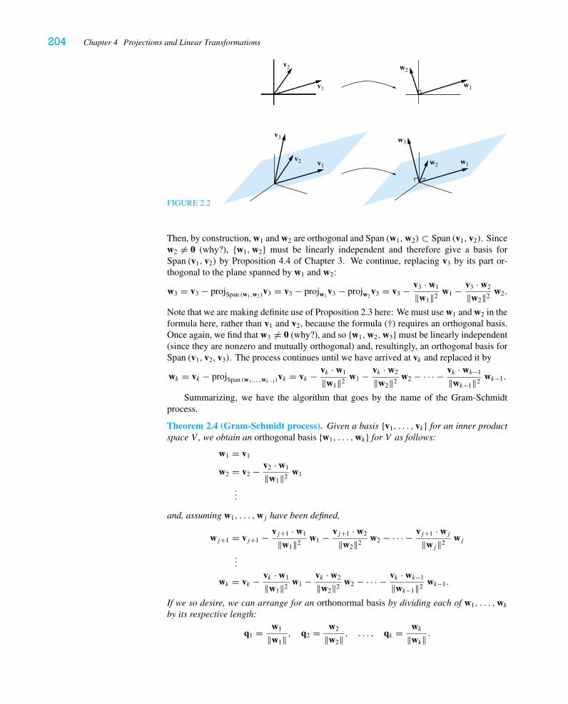
204 Chapter 4 Projections and Linear Transformations
FIGURE 2.2
v2
v1
w2
w1
v3
v2 v1
w3
w1w2
Then, by construction, w1 and w2 are orthogonal and Span (w1,w2) ⊂ Span (v1, v2). Sincew2 = 0 (why?), {w1,w2} must be linearly independent and therefore give a basis forSpan (v1, v2) by Proposition 4.4 of Chapter 3. We continue, replacing v3 by its part or-thogonal to the plane spanned by w1 and w2:
w3 = v3 − projSpan (w1,w2)v3 = v3 − projw1
v3 − projw2v3 = v3 − v3 · w1
‖w1‖2w1 − v3 · w2
‖w2‖2w2.
Note that we are making definite use of Proposition 2.3 here: We must use w1 and w2 in theformula here, rather than v1 and v2, because the formula (†) requires an orthogonal basis.Once again, we find that w3 = 0 (why?), and so {w1,w2,w3} must be linearly independent(since they are nonzero and mutually orthogonal) and, resultingly, an orthogonal basis forSpan (v1, v2, v3). The process continues until we have arrived at vk and replaced it by
wk = vk − projSpan (w1,...,wk−1)vk = vk − vk · w1
‖w1‖2w1 − vk · w2
‖w2‖2w2 − · · · − vk · wk−1
‖wk−1‖2wk−1.
Summarizing, we have the algorithm that goes by the name of the Gram-Schmidtprocess.
Theorem 2.4 (Gram-Schmidt process). Given a basis {v1, . . . , vk} for an inner productspace V , we obtain an orthogonal basis {w1, . . . ,wk} for V as follows:
w1 = v1
w2 = v2 − v2 · w1
‖w1‖2w1
...
and, assuming w1, . . . ,wj have been defined,
wj+1 = vj+1 − vj+1 · w1
‖w1‖2w1 − vj+1 · w2
‖w2‖2w2 − · · · − vj+1 · wj
‖wj‖2wj
...
wk = vk − vk · w1
‖w1‖2w1 − vk · w2
‖w2‖2w2 − · · · − vk · wk−1
‖wk−1‖2wk−1.
If we so desire, we can arrange for an orthonormal basis by dividing each of w1, . . . ,wkby its respective length:
q1 = w1
‖w1‖ , q2 = w2
‖w2‖ , . . . , qk = wk‖wk‖ .
2 Orthogonal Bases 205
EXAMPLE 2
Let v1 = (1, 1, 1, 1), v2 = (3, 1,−1, 1), and v3 = (1, 1, 3, 3). We want to use the Gram-Schmidt process to give an orthogonal basis for V = Span (v1, v2, v3) ⊂ R4. We take
w1 = v1 = (1, 1, 1, 1);w2 = v2 − v2 · w1
‖w1‖2w1 = (3, 1,−1, 1)− (3, 1,−1, 1) · (1, 1, 1, 1)
‖(1, 1, 1, 1)‖2(1, 1, 1, 1)
= (3, 1,−1, 1)− 4
4(1, 1, 1, 1) = (2, 0,−2, 0);
w3 = v3 − v3 · w1
‖w1‖2w1 − v3 · w2
‖w2‖2w2
= (1, 1, 3, 3)− (1, 1, 3, 3) · (1, 1, 1, 1)‖(1, 1, 1, 1)‖2
(1, 1, 1, 1)
− (1, 1, 3, 3) · (2, 0,−2, 0)
‖(2, 0,−2, 0)‖2(2, 0,−2, 0)
= (1, 1, 3, 3)− 8
4(1, 1, 1, 1)− −4
8(2, 0,−2, 0) = (0,−1, 0, 1).
And if we desire an orthonormal basis, then we take
q1 = 1
2(1, 1, 1, 1),
q2 = 1√2(1, 0,−1, 0),
q3 = 1√2(0,−1, 0, 1).
It’s always a good idea to check that the vectors form an orthogonal (or orthonormal) set,and it’s easy—with these numbers—to do so.
2.1 The QR DecompositionThe Gram-Schmidt process gives rise in an obvious way to another matrix decompositionthat is useful in numerical computation. Just as the reduction to echelon form led tothe LU decomposition, the Gram-Schmidt process gives us what is usually called theQR decomposition. We start with a matrix A whose columns v1, . . . , vn form a linearlyindependent set. Let q1, . . . ,qn be the orthonormal basis for C(A) obtained by applyingthe Gram-Schmidt process to v1, . . . , vn. Notice that for j = 1, . . . , n, the vector vj can bewritten as a linear combination of q1, q2, . . . ,qj (why?). Thus, if we let Q be the m× nmatrix with columns q1, . . . ,qn, we see that there is an upper triangular n× nmatrix R sothat A = QR. Moreover, R is nonsingular, since its diagonal entries are nonzero.
EXAMPLE 3
Revisiting Example 2 above, let
A =
⎡⎢⎢⎢⎢⎣
1 3 1
1 1 1
1 −1 3
1 1 3
⎤⎥⎥⎥⎥⎦, Q =
⎡⎢⎢⎢⎢⎢⎣
12
1√2
012 0 − 1√
212 − 1√
20
12 0 1√
2
⎤⎥⎥⎥⎥⎥⎦, and R =
⎡⎢⎢⎣
2 2 4
0 2√
2 −√2
0 0√
2
⎤⎥⎥⎦ .
206 Chapter 4 Projections and Linear Transformations
Then, as the reader can check, we have A = QR. The entries of R can be computed bykeeping track of the arithmetic during the Gram-Schmidt process, or, more easily, by notingthat rij = qi · vj . (Note, as a check, that rij = 0 whenever i > j .)
Remark. The fact that the columns of the m× n matrix Q form an orthonormal set canbe restated in matrix form as QTQ = In. When A is square, so is the matrix Q. Ann× nmatrixQ is called orthogonal if its column vectors form an orthonormal set,4 i.e., ifQTQ = In. Orthogonal matrices will have a geometric role to play soon and will reappearseriously in Chapter 6.
Remark. Suppose we have calculated theQR decomposition of an m× n matrix A whosecolumns form a linearly independent set. How does this help us deal with the normalequations and the projection formula? Recall that the normal equations are
(ATA)x = ATb;substituting A = QR, we have
RT(QTQ)Rx = RTQTb, or
Rx = QTb.
(Here we’ve used the facts that QTQ = In and that R is nonsingular, and hence RT isnonsingular.) In particular, using the formula
x = R−1QTb
to solve for the least squares solution is quite effective for computer work. Finally, theprojection matrix (∗) on p. 194 can be rewritten
PV = A(ATA)−1AT = (QR)(RTR)−1(RTQT) = (QR)(R−1)(RT)−1(RT)QT = QQT,
which says that projecting onto the subspace C(A) is the same as summing the projectionsonto the orthonormal basis vectors q1, . . . ,qn. This is exactly what Proposition 2.3 told us.
Exercises 4.2
1. Redo Exercise 4.1.4 by finding an orthogonal basis for V .
2. Execute the Gram-Schmidt process in each case to give an orthonormal basis for thesubspace spanned by the given vectors.a. (1, 0, 0), (2, 1, 0), (3, 2, 1)
b. (1, 1, 1), (0, 1, 1), (0, 0, 1)
c.∗ (1, 0, 1, 0), (2, 1, 0, 1), (0, 1, 2,−3)
d. (−1, 2, 0, 2), (2,−4, 1,−4), (−1, 3, 1, 1)
3. Let V = Span((2, 1, 0,−2), (3, 3, 1, 0)
) ⊂ R4.a. Find an orthogonal basis for V .
b. Use your answer to part a to find the projection of b = (0, 4,−4,−7) onto V .
c. Use your answer to part a to find the projection matrix PV .
4The terminology is confusing and unfortunate, but history has set it in stone. Matrices with orthogonal columnvectors of nonunit length don’t have a special name.
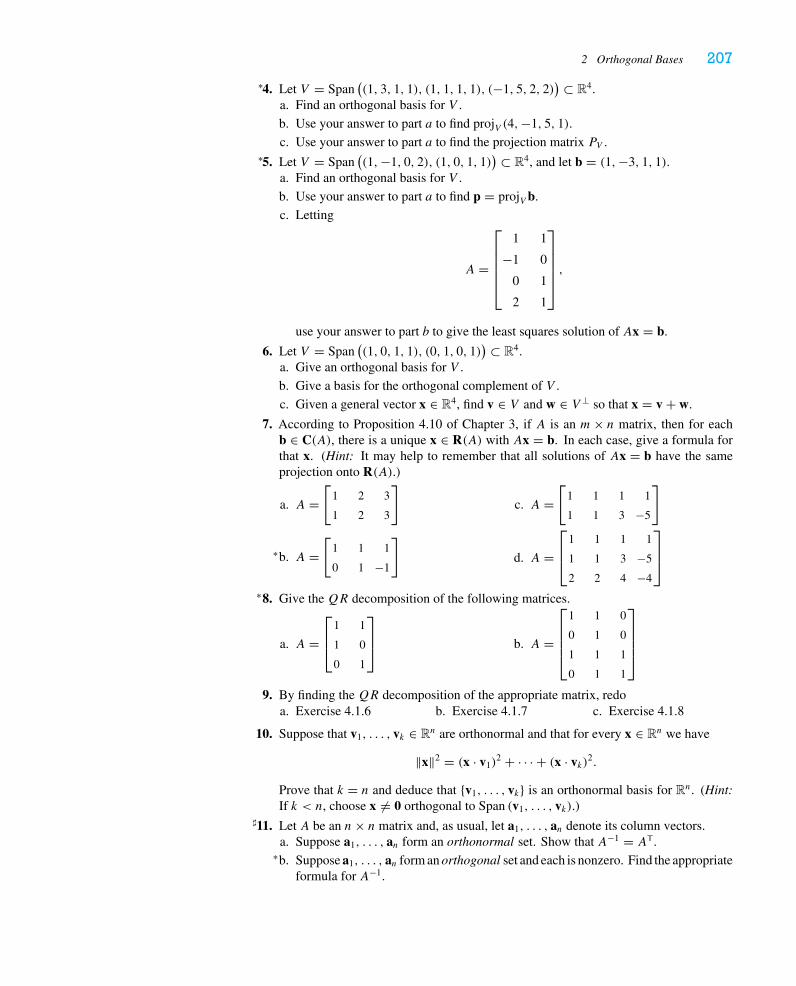
2 Orthogonal Bases 207
4.∗ Let V = Span((1, 3, 1, 1), (1, 1, 1, 1), (−1, 5, 2, 2)
) ⊂ R4.a. Find an orthogonal basis for V .
b. Use your answer to part a to find projV (4,−1, 5, 1).
c. Use your answer to part a to find the projection matrix PV .
5.∗ Let V = Span((1,−1, 0, 2), (1, 0, 1, 1)
) ⊂ R4, and let b = (1,−3, 1, 1).a. Find an orthogonal basis for V .
b. Use your answer to part a to find p = projV b.
c. Letting
A =
⎡⎢⎢⎢⎢⎣
1 1
−1 0
0 1
2 1
⎤⎥⎥⎥⎥⎦,
use your answer to part b to give the least squares solution of Ax = b.
6. Let V = Span((1, 0, 1, 1), (0, 1, 0, 1)
) ⊂ R4.a. Give an orthogonal basis for V .
b. Give a basis for the orthogonal complement of V .
c. Given a general vector x ∈ R4, find v ∈ V and w ∈ V ⊥ so that x = v + w.
7. According to Proposition 4.10 of Chapter 3, if A is an m× n matrix, then for eachb ∈ C(A), there is a unique x ∈ R(A) with Ax = b. In each case, give a formula forthat x. (Hint: It may help to remember that all solutions of Ax = b have the sameprojection onto R(A).)
a. A =[
1 2 3
1 2 3
]
b.∗ A =[
1 1 1
0 1 −1
]c. A =
[1 1 1 1
1 1 3 −5
]
d. A =⎡⎢⎣
1 1 1 1
1 1 3 −5
2 2 4 −4
⎤⎥⎦
8.∗ Give theQR decomposition of the following matrices.
a. A =⎡⎢⎣
1 1
1 0
0 1
⎤⎥⎦ b. A =
⎡⎢⎢⎢⎣
1 1 0
0 1 0
1 1 1
0 1 1
⎤⎥⎥⎥⎦
9. By finding theQR decomposition of the appropriate matrix, redoa. Exercise 4.1.6 b. Exercise 4.1.7 c. Exercise 4.1.8
10. Suppose that v1, . . . , vk ∈ Rn are orthonormal and that for every x ∈ Rn we have
‖x‖2 = (x · v1)2 + · · · + (x · vk)2.
Prove that k = n and deduce that {v1, . . . , vk} is an orthonormal basis for Rn. (Hint:If k < n, choose x = 0 orthogonal to Span (v1, . . . , vk).)
11.� Let A be an n× n matrix and, as usual, let a1, . . . , an denote its column vectors.a. Suppose a1, . . . , an form an orthonormal set. Show that A−1 = AT.
b.∗ Suppose a1, . . . , an form an orthogonal set and each is nonzero. Find the appropriateformula for A−1.
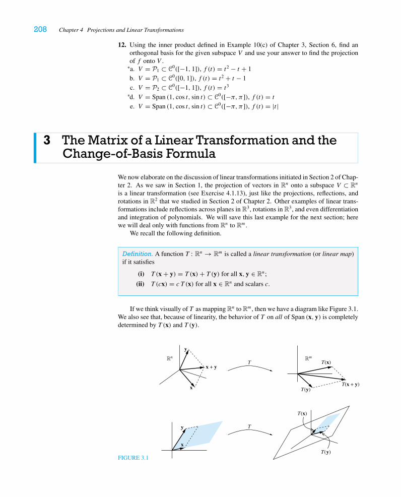
208 Chapter 4 Projections and Linear Transformations
12. Using the inner product defined in Example 10(c) of Chapter 3, Section 6, find anorthogonal basis for the given subspace V and use your answer to find the projectionof f onto V .a.∗ V = P1 ⊂ C0([−1, 1]), f (t) = t2 − t + 1
b. V = P1 ⊂ C0([0, 1]), f (t) = t2 + t − 1
c. V = P2 ⊂ C0([−1, 1]), f (t) = t3
d.∗ V = Span (1, cos t, sin t) ⊂ C0([−π, π ]), f (t) = t
e. V = Span (1, cos t, sin t) ⊂ C0([−π, π ]), f (t) = |t |
3 TheMatrix of a Linear Transformation and theChange-of-Basis Formula
We now elaborate on the discussion of linear transformations initiated in Section 2 of Chap-ter 2. As we saw in Section 1, the projection of vectors in Rn onto a subspace V ⊂ Rn
is a linear transformation (see Exercise 4.1.13), just like the projections, reflections, androtations in R2 that we studied in Section 2 of Chapter 2. Other examples of linear trans-formations include reflections across planes in R3, rotations in R3, and even differentiationand integration of polynomials. We will save this last example for the next section; herewe will deal only with functions from Rn to Rm.
We recall the following definition.
Definition. A function T : Rn → Rm is called a linear transformation (or linear map)if it satisfies
(i) T (x + y) = T (x)+ T (y) for all x, y ∈ Rn;
(ii) T (cx) = c T (x) for all x ∈ Rn and scalars c.
If we think visually of T as mapping Rn to Rm, then we have a diagram like Figure 3.1.We also see that, because of linearity, the behavior of T on all of Span (x, y) is completelydetermined by T (x) and T (y).
FIGURE 3.1
x
y
T
T
x
y
Rn Rm
x + y
T(y)
T(x)
T(x)
T(y)T(x + y)
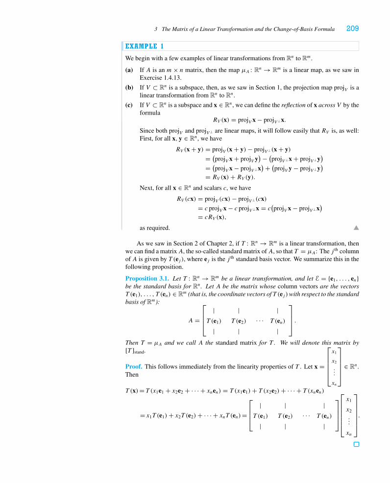
3 The Matrix of a Linear Transformation and the Change-of-Basis Formula 209
EXAMPLE 1
We begin with a few examples of linear transformations from Rn to Rm.
(a) If A is an m× n matrix, then the map μA : Rn → Rm is a linear map, as we saw inExercise 1.4.13.
(b) If V ⊂ Rn is a subspace, then, as we saw in Section 1, the projection map projV is alinear transformation from Rn to Rn.
(c) If V ⊂ Rn is a subspace and x ∈ Rn, we can define the reflection of x across V by theformula
RV (x) = projV x − projV ⊥x.
Since both projV and projV ⊥ are linear maps, it will follow easily that RV is, as well:First, for all x, y ∈ Rn, we have
RV (x + y) = projV (x + y)− projV ⊥(x + y)
= (projV x + projV y)− (projV ⊥x + projV ⊥y
)= (projV x − projV ⊥x
)+ (projV y − projV ⊥y)
= RV (x)+ RV (y).Next, for all x ∈ Rn and scalars c, we have
RV (cx) = projV (cx)− projV ⊥(cx)
= c projV x − c projV ⊥x = c(projV x − projV ⊥x
)= cRV (x),
as required.
As we saw in Section 2 of Chapter 2, if T : Rn → Rm is a linear transformation, thenwe can find a matrixA, the so-called standard matrix ofA, so that T = μA: The j th columnof A is given by T (ej ), where ej is the j th standard basis vector. We summarize this in thefollowing proposition.
Proposition 3.1. Let T : Rn → Rm be a linear transformation, and let E = {e1, . . . , en}be the standard basis for Rn. Let A be the matrix whose column vectors are the vectorsT (e1), . . . , T (en) ∈ Rm (that is, the coordinate vectors of T (ej )with respect to the standardbasis of Rm):
A =
⎡⎢⎢⎣
|T (e1)
|
|T (e2)
|· · ·
|T (en)
|
⎤⎥⎥⎦ .
Then T = μA and we call A the standard matrix for T . We will denote this matrix by[T ]stand.
Proof. This follows immediately from the linearity properties of T . Let x =
⎡⎢⎢⎢⎢⎣
x1
x2
...
xn
⎤⎥⎥⎥⎥⎦
∈ Rn.Then
T (x)= T (x1e1 + x2e2 + · · · + xnen) = T (x1e1)+ T (x2e2)+ · · · + T (xnen)
= x1T (e1)+ x2T (e2)+ · · · + xnT (en)=
⎡⎢⎢⎣
|T (e1)
|
|T (e2)
|· · ·
|T (en)
|
⎤⎥⎥⎦
⎡⎢⎢⎢⎢⎢⎣
x1
x2
...
xn
⎤⎥⎥⎥⎥⎥⎦.
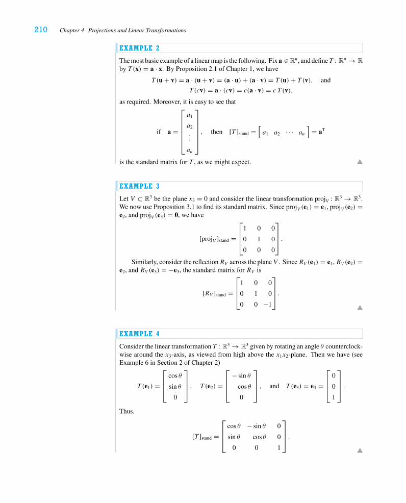
210 Chapter 4 Projections and Linear Transformations
EXAMPLE 2
The most basic example of a linear map is the following. Fix a ∈ Rn, and defineT : Rn → R
by T (x) = a · x. By Proposition 2.1 of Chapter 1, we have
T (u + v) = a · (u + v) = (a · u)+ (a · v) = T (u)+ T (v), and
T (cv) = a · (cv) = c(a · v) = c T (v),
as required. Moreover, it is easy to see that
if a =
⎡⎢⎢⎢⎢⎢⎣
a1
a2
...
an
⎤⎥⎥⎥⎥⎥⎦, then [T ]stand =
[a1 a2 · · · an
]= aT
is the standard matrix for T , as we might expect.
EXAMPLE 3
Let V ⊂ R3 be the plane x3 = 0 and consider the linear transformation projV : R3 → R3.We now use Proposition 3.1 to find its standard matrix. Since projV (e1) = e1, projV (e2) =e2, and projV (e3) = 0, we have
[projV ]stand =
⎡⎢⎢⎣
1 0 0
0 1 0
0 0 0
⎤⎥⎥⎦ .
Similarly, consider the reflectionRV across the planeV . SinceRV (e1) = e1,RV (e2) =e2, and RV (e3) = −e3, the standard matrix for RV is
[RV ]stand =
⎡⎢⎢⎣
1 0 0
0 1 0
0 0 −1
⎤⎥⎥⎦ .
EXAMPLE 4
Consider the linear transformation T : R3 → R3 given by rotating an angle θ counterclock-wise around the x3-axis, as viewed from high above the x1x2-plane. Then we have (seeExample 6 in Section 2 of Chapter 2)
T (e1) =
⎡⎢⎢⎣
cos θ
sin θ
0
⎤⎥⎥⎦ , T (e2) =
⎡⎢⎢⎣
− sin θ
cos θ
0
⎤⎥⎥⎦ , and T (e3) = e3 =
⎡⎢⎢⎣
0
0
1
⎤⎥⎥⎦ .
Thus,
[T ]stand =
⎡⎢⎢⎣
cos θ − sin θ 0
sin θ cos θ 0
0 0 1
⎤⎥⎥⎦ .
3 The Matrix of a Linear Transformation and the Change-of-Basis Formula 211
EXAMPLE 5
Now let V ⊂ R3 be the plane spanned by v1 =⎡⎢⎣
1
0
1
⎤⎥⎦ and v2 =
⎡⎢⎣
1
1
−1
⎤⎥⎦. Let’s compute the
standard matrix for projV using Proposition 3.1. Noting that {v1, v2} gives an orthogonalbasis for V , we can use Proposition 2.3 to compute
projV (e1) = projv1(e1)+ projv2
(e1)
= 1
2
⎡⎢⎢⎣
1
0
1
⎤⎥⎥⎦+ 1
3
⎡⎢⎢⎣
1
1
−1
⎤⎥⎥⎦ = 1
6
⎡⎢⎢⎣
5
2
1
⎤⎥⎥⎦ ,
projV (e2) = projv1(e2)+ projv2
(e2)
= 0
2
⎡⎢⎢⎣
1
0
1
⎤⎥⎥⎦+ 1
3
⎡⎢⎢⎣
1
1
−1
⎤⎥⎥⎦ = 1
3
⎡⎢⎢⎣
1
1
−1
⎤⎥⎥⎦ , and
projV (e3) = projv1(e3)+ projv2
(e3)
= 1
2
⎡⎢⎢⎣
1
0
1
⎤⎥⎥⎦+ −1
3
⎡⎢⎢⎣
1
1
−1
⎤⎥⎥⎦ = 1
6
⎡⎢⎢⎣
1
−2
5
⎤⎥⎥⎦ .
Thus, the standard matrix for projV is given by
[projV ]stand = 1
6
⎡⎢⎢⎣
5 2 1
2 2 −2
1 −2 5
⎤⎥⎥⎦ .
Of course, in general, [projV ]stand is nothing but the projection matrix PV we computed inSection 1.
EXAMPLE 6
Using the same plane V as in Example 5, we can compute the standard matrix for projV ⊥because we know that projV + projV ⊥ is the identity map. Thus, the standard matrix forprojV ⊥ is given by
[projV ⊥]stand =
⎡⎢⎢⎣
1 0 0
0 1 0
0 0 1
⎤⎥⎥⎦− 1
6
⎡⎢⎢⎣
5 2 1
2 2 −2
1 −2 5
⎤⎥⎥⎦ = 1
6
⎡⎢⎢⎣
1 −2 −1
−2 4 2
−1 2 1
⎤⎥⎥⎦ .
To double-check our work, note that the column space (and row space, too) is spanned by
v3 =⎡⎢⎣
1
−2
−1
⎤⎥⎦, which is orthogonal to v1 and v2 and therefore spans V ⊥.
212 Chapter 4 Projections and Linear Transformations
Similarly, we can compute the standard matrix for reflection across V by using thedefinition:
[RV ]stand = [projV ]stand − [projV ⊥]stand
= 1
6
⎡⎢⎢⎣
5 2 1
2 2 −2
1 −2 5
⎤⎥⎥⎦− 1
6
⎡⎢⎢⎣
1 −2 −1
−2 4 2
−1 2 1
⎤⎥⎥⎦ = 1
6
⎡⎢⎢⎣
4 4 2
4 −2 −4
2 −4 4
⎤⎥⎥⎦
= 1
3
⎡⎢⎢⎣
2 2 1
2 −1 −2
1 −2 2
⎤⎥⎥⎦ .
We see in these examples that the standard matrix for a projection or reflection maydisguise the geometry of the actual linear transformation. When x ∈ V and y ∈ V ⊥, weknow that projV (x) = x and projV (y) = 0; thus, in Example 5, since v1, v2 ∈ V and v3 ∈V ⊥, we have
projV (v1) = v1,
projV (v2) = v2,
projV (v3) = 0.
Now, since v1, v2, and v3 are mutually orthogonal nonzero vectors, they form a basis forR3. Thus, given any x ∈ R3, we can write x = c1v1 + c2v2 + c3v3 for appropriate scalarsc1, c2, and c3. Since projV is a linear transformation, we therefore have
projV (x) = projV (c1v1 + c2v2 + c3v3)
= c1projV (v1)+ c2projV (v2)+ c3projV (v3)
= c1v1 + c2v2.
Similarly, when x ∈ V and y ∈ V ⊥, we know that RV (x) = x and RV (y) = −y, so
RV (x) = RV (c1v1 + c2v2 + c3v3) = c1v1 + c2v2 − c3v3.
These examples lead us to make the following definition.
Definition. Let T : Rn → Rn be a linear transformation, and let B = {v1, . . . , vn} be anordered basis for Rn. For each j = 1, . . . , n, let a1j , a2j , . . . , anj denote the coordinatesof T (vj ) with respect to the basis B, i.e.,
T (vj ) = a1jv1 + a2jv2 + · · · + anjvn, j = 1, . . . , n.
Then we define A = [aij ] to be the matrix for T with respect to the basis B. We denotethis matrix by [T ]B.
It is important to remember that the coefficients of T (vj ) will be entered as the j th
column of the matrix [T ]B. To write this formally, given a vector x ∈ Rn, we let CB(x)denote the column vector whose entries are the coordinates of x with respect to the basis
3 The Matrix of a Linear Transformation and the Change-of-Basis Formula 213
B. That is, if
x = c1v1 + c2v2 + · · · + cnvn, then CB(x) =
⎡⎢⎢⎢⎢⎢⎣
c1
c2
...
cn
⎤⎥⎥⎥⎥⎥⎦.
With this notation, we now can write
[T ]B =
⎡⎢⎢⎣
|CB(T (v1))
|
|CB(T (v2))
|· · ·
|CB(T (vn))
|
⎤⎥⎥⎦ .
Remark. If we denote the standard basis {e1, . . . , en} by E, we have [T ]E = [T ]stand.
EXAMPLE 7
Returning to Examples 5 and 6, when we take B = {v1, v2, v3}, with
v1 =
⎡⎢⎢⎣
1
0
1
⎤⎥⎥⎦ , v2 =
⎡⎢⎢⎣
1
1
−1
⎤⎥⎥⎦ , and v3 =
⎡⎢⎢⎣
1
−2
−1
⎤⎥⎥⎦
and V = Span (v1, v2), we have
[projV ]B =
⎡⎢⎢⎣
1 0 0
0 1 0
0 0 0
⎤⎥⎥⎦ , [projV ⊥]B =
⎡⎢⎢⎣
0 0 0
0 0 0
0 0 1
⎤⎥⎥⎦ ,
and [RV ]B =
⎡⎢⎢⎣
1 0 0
0 1 0
0 0 −1
⎤⎥⎥⎦ .
In fact, it doesn’t matter what the particular vectors v1, v2, and v3 happen to be. So longas V = Span (v1, v2) and V ⊥ = Span (v3), we will obtain these matrices with respect tothe basis B. Indeed, these are the matrices we obtained for projection onto and reflectionacross the standard plane x3 = 0 in Example 3.
EXAMPLE 8
Let T : R2 → R2 be the linear transformation defined by multiplying by
A =[
3 1
2 2
].
It is rather difficult to understand this mapping until we discover that if we take
v1 =[
1
1
]and v2 =
[−1
2
],
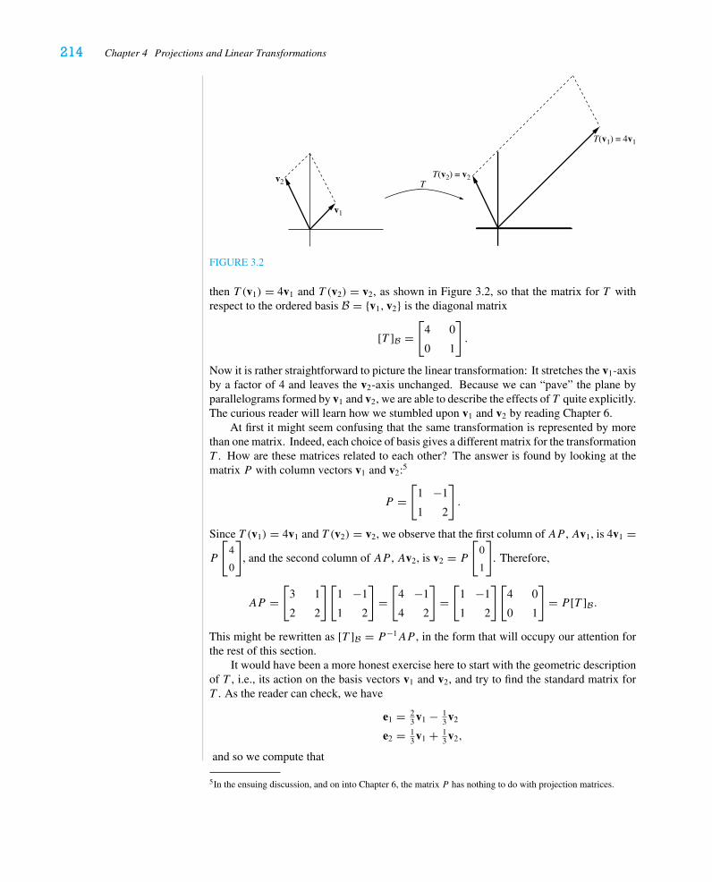
214 Chapter 4 Projections and Linear Transformations
v2
v1
T(v2) = v2
T(v1) = 4v1
T
FIGURE 3.2
then T (v1) = 4v1 and T (v2) = v2, as shown in Figure 3.2, so that the matrix for T withrespect to the ordered basis B = {v1, v2} is the diagonal matrix
[T ]B =[
4 0
0 1
].
Now it is rather straightforward to picture the linear transformation: It stretches the v1-axisby a factor of 4 and leaves the v2-axis unchanged. Because we can “pave” the plane byparallelograms formed by v1 and v2, we are able to describe the effects of T quite explicitly.The curious reader will learn how we stumbled upon v1 and v2 by reading Chapter 6.
At first it might seem confusing that the same transformation is represented by morethan one matrix. Indeed, each choice of basis gives a different matrix for the transformationT . How are these matrices related to each other? The answer is found by looking at thematrix P with column vectors v1 and v2:5
P =[
1 −1
1 2
].
Since T (v1) = 4v1 and T (v2) = v2, we observe that the first column of AP , Av1, is 4v1 =P
[4
0
], and the second column of AP , Av2, is v2 = P
[0
1
]. Therefore,
AP =[
3 1
2 2
][1 −1
1 2
]=[
4 −1
4 2
]=[
1 −1
1 2
][4 0
0 1
]= P [T ]B.
This might be rewritten as [T ]B = P−1AP , in the form that will occupy our attention forthe rest of this section.
It would have been a more honest exercise here to start with the geometric descriptionof T , i.e., its action on the basis vectors v1 and v2, and try to find the standard matrix forT . As the reader can check, we have
e1 = 23 v1 − 1
3 v2
e2 = 13 v1 + 1
3 v2,
and so we compute that
5In the ensuing discussion, and on into Chapter 6, the matrix P has nothing to do with projection matrices.
3 The Matrix of a Linear Transformation and the Change-of-Basis Formula 215
T (e1) = 23T (v1)− 1
3T (v2) = 83 v1 − 1
3 v2
=[
3
2
], and
T (e2) = 13T (v1)+ 1
3T (v2) = 43 v1 + 1
3 v2
=[
1
2
].
What a relief! In matrix form, this would, of course, be the equation A = [T ]stand =P [T ]BP−1.
Following this example, we now state the main result of this section.
Proposition 3.2 (Change-of-Basis Formula, Take 1). Let T : Rn → Rn be a linear trans-formation with standard matrix [T ]stand. Let B = {v1, . . . , vn} be an ordered basis for Rn
and let [T ]B be the matrix for T with respect to B. LetP be the n× nmatrix whose columnsare given by the vectors v1, . . . , vn. Then we have
[T ]standP = P [T ]B.
Remark. Since P is invertible (why?), this can be written as [T ]stand = P [T ]BP−1 or as[T ]B = P−1[T ]standP , providing us formulas to find [T ]stand from [T ]B, and vice versa.Since these formulas tell us how to change the matrix from one basis to another, we callthem change-of-basis formulas. We call P the change-of-basis matrix from the standardbasis to the basis B. Note that, as a linear transformation,
μP (ej ) = vj , j = 1, . . . , n;that is, it maps the j th standard basis vector to the j th element of the new ordered basis.
Proof. The j th column of P is the vector vj (more specifically, its coordinate vectorCE(vj )with respect to the standard basis). Therefore, the j th column vector of the matrix product[T ]standP is the standard coordinate vector of T (vj ). On the other hand, the j th column of[T ]B is the coordinate vector, CB(T (vj )), of T (vj ) with respect to the basis B. That is,
if the j th column of [T ]B is
⎡⎢⎢⎢⎢⎣
α1
α2
...
αn
⎤⎥⎥⎥⎥⎦
then T (vj ) = α1v1 + α2v2 + · · · + αnvn. But we alsoknow that
P
⎡⎢⎢⎢⎢⎢⎣
α1
α2
...
αn
⎤⎥⎥⎥⎥⎥⎦
= α1v1 + α2v2 + · · · + αnvn.
That is, the j th column of P [T ]B is exactly the linear combination of the columns of Pneeded to give the standard coordinate vector of T (vj ).
216 Chapter 4 Projections and Linear Transformations
EXAMPLE 9
We want to use the change-of-basis formula, Proposition 3.2, and the result of Example 7to recover the results of Examples 5 and 6. Starting with the basis B = {v1, v2, v3}, with
v1 =
⎡⎢⎢⎣
1
0
1
⎤⎥⎥⎦ , v2 =
⎡⎢⎢⎣
1
1
−1
⎤⎥⎥⎦ , and v3 =
⎡⎢⎢⎣
1
−2
−1
⎤⎥⎥⎦ ,
we note that V = Span (v1, v2) and so
[projV ]B =
⎡⎢⎢⎣
1 0 0
0 1 0
0 0 0
⎤⎥⎥⎦ .
To get the standard matrix for projV , we take
P =
⎡⎢⎢⎣
| | |v1 v2 v3
| | |
⎤⎥⎥⎦ =
⎡⎢⎢⎣
1 1 1
0 1 −2
1 −1 −1
⎤⎥⎥⎦
and compute that
P−1 = 1
6
⎡⎢⎢⎣
3 0 3
2 2 −2
1 −2 −1
⎤⎥⎥⎦ .
(Exercise 4.2.11 may be helpful here, but, as a last resort, there’s always Gaussian elimi-nation.) Then we have
[projV ]stand = P [projV ]BP−1 = 1
6
⎡⎢⎢⎣
1 1 1
0 1 −2
1 −1 −1
⎤⎥⎥⎦
⎡⎢⎢⎣
1 0 0
0 1 0
0 0 0
⎤⎥⎥⎦
⎡⎢⎢⎣
3 0 3
2 2 −2
1 −2 −1
⎤⎥⎥⎦
= 1
6
⎡⎢⎢⎣
5 2 1
2 2 −2
1 −2 5
⎤⎥⎥⎦ ,
as before. Similarly,
[RV ]stand = P [RV ]BP−1 = 1
6
⎡⎢⎢⎣
1 1 1
0 1 −2
1 −1 −1
⎤⎥⎥⎦
⎡⎢⎢⎣
1 0 0
0 1 0
0 0 −1
⎤⎥⎥⎦
⎡⎢⎢⎣
3 0 3
2 2 −2
1 −2 −1
⎤⎥⎥⎦
= 1
3
⎡⎢⎢⎣
2 2 1
2 −1 −2
1 −2 2
⎤⎥⎥⎦ ,
just as we obtained previously.
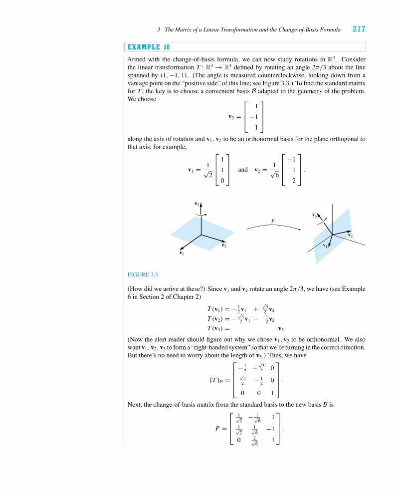
3 The Matrix of a Linear Transformation and the Change-of-Basis Formula 217
EXAMPLE 10
Armed with the change-of-basis formula, we can now study rotations in R3. Considerthe linear transformation T : R3 → R3 defined by rotating an angle 2π/3 about the linespanned by (1,−1, 1). (The angle is measured counterclockwise, looking down from avantage point on the “positive side” of this line; see Figure 3.3.) To find the standard matrixfor T , the key is to choose a convenient basis B adapted to the geometry of the problem.We choose
v3 =
⎡⎢⎢⎣
1
−1
1
⎤⎥⎥⎦
along the axis of rotation and v1, v2 to be an orthonormal basis for the plane orthogonal tothat axis; for example,
v1 = 1√2
⎡⎢⎢⎣
1
1
0
⎤⎥⎥⎦ and v2 = 1√
6
⎡⎢⎢⎣
−1
1
2
⎤⎥⎥⎦ .
e3
e2
e1
v3
v2
v1
P
FIGURE 3.3
(How did we arrive at these?) Since v1 and v2 rotate an angle 2π/3, we have (see Example6 in Section 2 of Chapter 2)
T (v1) = − 12 v1 +
√3
2 v2
T (v2) = −√
32 v1 − 1
2 v2
T (v3) = v3.
(Now the alert reader should figure out why we chose v1, v2 to be orthonormal. We alsowant v1, v2, v3 to form a “right-handed system” so that we’re turning in the correct direction.But there’s no need to worry about the length of v3.) Thus, we have
[T ]B =
⎡⎢⎢⎢⎣
− 12 −
√3
2 0√
32 − 1
2 0
0 0 1
⎤⎥⎥⎥⎦ .
Next, the change-of-basis matrix from the standard basis to the new basis B is
P =
⎡⎢⎢⎣
1√2
− 1√6
1
1√2
1√6
−1
0 2√6
1
⎤⎥⎥⎦ ,
218 Chapter 4 Projections and Linear Transformations
whose inverse matrix is
P−1 =
⎡⎢⎢⎣
1√2
1√2
0
− 1√6
1√6
2√6
13 − 1
313
⎤⎥⎥⎦ .
Once again, we solve for
[T ]stand = P [T ]BP−1 =
⎡⎢⎢⎣
1√2
− 1√6
1
1√2
1√6
−1
0 2√6
1
⎤⎥⎥⎦
⎡⎢⎢⎣
− 12 −
√3
2 0√
32 − 1
2 0
0 0 1
⎤⎥⎥⎦
⎡⎢⎢⎣
1√2
1√2
0
− 1√6
1√6
2√6
13 − 1
313
⎤⎥⎥⎦
=
⎡⎢⎢⎣
0 −1 0
0 0 −1
1 0 0
⎤⎥⎥⎦ ,
amazingly enough. In hindsight, then, we should be able to see the effect of T on thestandard basis vectors quite plainly. Can you?
Remark. Suppose we first rotateπ/2 about the x3-axis and then rotateπ/2 about the x1-axis.We leave it to the reader to check, in Exercise 2, that the result is the linear transformationwhose matrix we just calculated. This raises a fascinating question: Is the composition ofrotations always again a rotation? (See Exercise 6.2.16.) If so, is there a way of predictingthe ultimate axis and angle?
EXAMPLE 11
Consider the ordered basis B = {v1, v2, v3}, where
v1 =
⎡⎢⎢⎣
1
0
1
⎤⎥⎥⎦ , v2 =
⎡⎢⎢⎣
1
1
3
⎤⎥⎥⎦ , and v3 =
⎡⎢⎢⎣
1
−2
−2
⎤⎥⎥⎦ .
Suppose that T : R3 → R3 is the linear transformation defined by
T (v1) = v2 − v3, T (v2) = −v2, and T (v3) = v1 + v2.
Then the matrix [T ]B for T with respect to the basis B is given by
[T ]B =
⎡⎢⎢⎣
0 0 1
1 −1 1
−1 0 0
⎤⎥⎥⎦ .
To compute the standard matrix for T , we take
P =
⎡⎢⎢⎣
1 1 1
0 1 −2
1 3 −2
⎤⎥⎥⎦
3 The Matrix of a Linear Transformation and the Change-of-Basis Formula 219
and calculate
P−1 =
⎡⎢⎢⎣
4 5 −3
−2 −3 2
−1 −2 1
⎤⎥⎥⎦ .
Then
[T ]stand = P [T ]BP−1 =
⎡⎢⎢⎣
1 1 1
0 1 −2
1 3 −2
⎤⎥⎥⎦
⎡⎢⎢⎣
0 0 1
1 −1 1
−1 0 0
⎤⎥⎥⎦
⎡⎢⎢⎣
4 5 −3
−2 −3 2
−1 −2 1
⎤⎥⎥⎦
=
⎡⎢⎢⎣
0 −1 0
13 16 −10
22 26 −17
⎤⎥⎥⎦ .
We end this section with a definition and a few comments.
Definition. Let A and B be n× n matrices. We say B is similar to A if there is aninvertible matrix P such that B = P−1AP .
That is, two square matrices are similar if they are the matrices for some linear trans-formation with respect to different ordered bases.
We say a linear transformation T : V → V is diagonalizable if there is some basis Bfor V such that the matrix for T with respect to that basis is diagonal. Similarly,6 we say asquare matrix is diagonalizable if it is similar to a diagonal matrix. In Chapter 6 we willsee the power of diagonalizing matrices to solve a wide variety of problems, and we willlearn some convenient criteria for matrices to be diagonalizable.
EXAMPLE 12
Consider the matrices
A =[
2 1
0 3
]and B =
[2 0
0 3
].
To decide whether B is similar to A, we try to find an invertible matrix
P =[a b
c d
]
so that B = P−1AP , or, equivalently, PB = AP . Calculating, we have[a b
c d
][2 0
0 3
]=[
2 1
0 3
][a b
c d
]
[2a 3b
2c 3d
]=[
2a + c 2b + d3c 3d
]
6One of the authors apologizes for the atrocious pun; the other didn’t even notice.
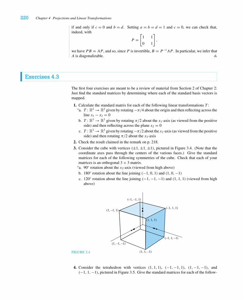
220 Chapter 4 Projections and Linear Transformations
if and only if c = 0 and b = d. Setting a = b = d = 1 and c = 0, we can check that,indeed, with
P =[
1 1
0 1
],
we have PB = AP , and so, since P is invertible, B = P−1AP . In particular, we infer thatA is diagonalizable.
Exercises 4.3
The first four exercises are meant to be a review of material from Section 2 of Chapter 2:Just find the standard matrices by determining where each of the standard basis vectors ismapped.
1. Calculate the standard matrix for each of the following linear transformations T :a.∗ T : R2 → R2 given by rotating −π/4 about the origin and then reflecting across the
line x1 − x2 = 0
b. T : R3 → R3 given by rotating π/2 about the x1-axis (as viewed from the positiveside) and then reflecting across the plane x2 = 0
c. T : R3 → R3 given by rotating −π/2 about the x1-axis (as viewed from the positiveside) and then rotating π/2 about the x3-axis
2. Check the result claimed in the remark on p. 218.
3. Consider the cube with vertices (±1,±1,±1), pictured in Figure 3.4. (Note that thecoordinate axes pass through the centers of the various faces.) Give the standardmatrices for each of the following symmetries of the cube. Check that each of yourmatrices is an orthogonal 3 × 3 matrix.a.∗ 90◦ rotation about the x3-axis (viewed from high above)
b. 180◦ rotation about the line joining (−1, 0, 1) and (1, 0,−1)
c. 120◦ rotation about the line joining (−1,−1,−1) and (1, 1, 1) (viewed from highabove)
FIGURE 3.4
(–1, 1, 1)(1, –1, 1)
(–1, –1, 1)
(–1, 1, –1)
(1, 1, 1)
(1, 1, –1)
(1, –1, –1)
4. Consider the tetrahedron with vertices (1, 1, 1), (−1,−1, 1), (1,−1,−1), and(−1, 1,−1), pictured in Figure 3.5. Give the standard matrices for each of the follow-
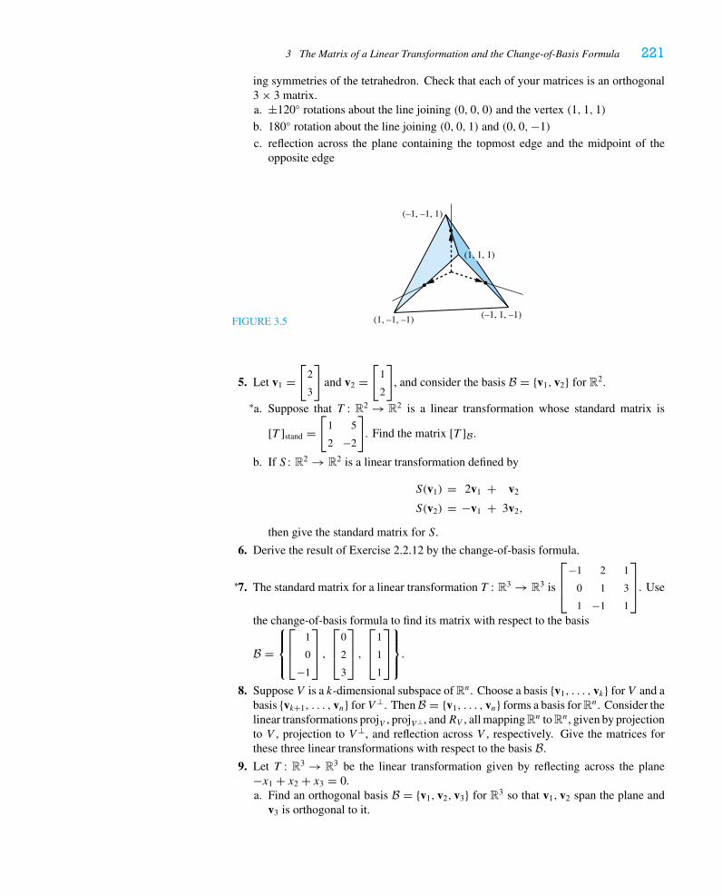
3 The Matrix of a Linear Transformation and the Change-of-Basis Formula 221
ing symmetries of the tetrahedron. Check that each of your matrices is an orthogonal3 × 3 matrix.a. ±120◦ rotations about the line joining (0, 0, 0) and the vertex (1, 1, 1)
b. 180◦ rotation about the line joining (0, 0, 1) and (0, 0,−1)
c. reflection across the plane containing the topmost edge and the midpoint of theopposite edge
FIGURE 3.5
(1, 1, 1)
(–1, 1, –1)(1, –1, –1)
(–1, –1, 1)
5. Let v1 =[
2
3
]and v2 =
[1
2
], and consider the basis B = {v1, v2} for R2.
a.∗ Suppose that T : R2 → R2 is a linear transformation whose standard matrix is
[T ]stand =[
1 5
2 −2
]. Find the matrix [T ]B.
b. If S : R2 → R2 is a linear transformation defined by
S(v1) = 2v1 + v2
S(v2) = −v1 + 3v2,
then give the standard matrix for S.
6. Derive the result of Exercise 2.2.12 by the change-of-basis formula.
7.∗ The standard matrix for a linear transformation T : R3 → R3 is
⎡⎢⎣
−1 2 1
0 1 3
1 −1 1
⎤⎥⎦. Use
the change-of-basis formula to find its matrix with respect to the basis
B =
⎧⎪⎨⎪⎩
⎡⎢⎣
1
0
−1
⎤⎥⎦ ,
⎡⎢⎣
0
2
3
⎤⎥⎦ ,
⎡⎢⎣
1
1
1
⎤⎥⎦
⎫⎪⎬⎪⎭
.
8. Suppose V is a k-dimensional subspace of Rn. Choose a basis {v1, . . . , vk} for V and abasis {vk+1, . . . , vn} for V ⊥. Then B = {v1, . . . , vn} forms a basis for Rn. Consider thelinear transformations projV , projV ⊥ , andRV , all mapping Rn to Rn, given by projectionto V , projection to V ⊥, and reflection across V , respectively. Give the matrices forthese three linear transformations with respect to the basis B.
9. Let T : R3 → R3 be the linear transformation given by reflecting across the plane−x1 + x2 + x3 = 0.a. Find an orthogonal basis B = {v1, v2, v3} for R3 so that v1, v2 span the plane and
v3 is orthogonal to it.
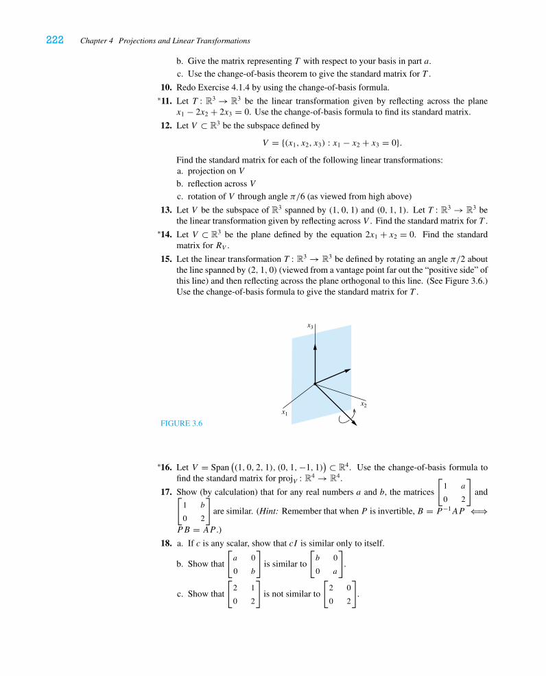
222 Chapter 4 Projections and Linear Transformations
b. Give the matrix representing T with respect to your basis in part a.
c. Use the change-of-basis theorem to give the standard matrix for T .
10. Redo Exercise 4.1.4 by using the change-of-basis formula.
11.∗ Let T : R3 → R3 be the linear transformation given by reflecting across the planex1 − 2x2 + 2x3 = 0. Use the change-of-basis formula to find its standard matrix.
12. Let V ⊂ R3 be the subspace defined by
V = {(x1, x2, x3) : x1 − x2 + x3 = 0}.Find the standard matrix for each of the following linear transformations:a. projection on V
b. reflection across V
c. rotation of V through angle π/6 (as viewed from high above)
13. Let V be the subspace of R3 spanned by (1, 0, 1) and (0, 1, 1). Let T : R3 → R3 bethe linear transformation given by reflecting across V . Find the standard matrix for T .
14.∗ Let V ⊂ R3 be the plane defined by the equation 2x1 + x2 = 0. Find the standardmatrix for RV .
15. Let the linear transformation T : R3 → R3 be defined by rotating an angle π/2 aboutthe line spanned by (2, 1, 0) (viewed from a vantage point far out the “positive side” ofthis line) and then reflecting across the plane orthogonal to this line. (See Figure 3.6.)Use the change-of-basis formula to give the standard matrix for T .
FIGURE 3.6
x1
x3
x2
16.∗ Let V = Span((1, 0, 2, 1), (0, 1,−1, 1)
) ⊂ R4. Use the change-of-basis formula tofind the standard matrix for projV : R4 → R4.
17. Show (by calculation) that for any real numbers a and b, the matrices
[1 a
0 2
]and[
1 b
0 2
]are similar. (Hint: Remember that when P is invertible, B = P−1AP ⇐⇒
PB = AP .)
18. a. If c is any scalar, show that cI is similar only to itself.
b. Show that
[a 0
0 b
]is similar to
[b 0
0 a
].
c. Show that
[2 1
0 2
]is not similar to
[2 0
0 2
].
3 The Matrix of a Linear Transformation and the Change-of-Basis Formula 223
d. Show that
[2 1
0 2
]is not diagonalizable, i.e., is not similar to any diagonal matrix.
(Hint: Remember that when P is invertible, B = P−1AP ⇐⇒ PB = AP .)
19. Let e1, e2 denote the standard basis, as usual. Let T : R2 → R2 be defined by
T (e1) = 8e1 − 4e2
T (e2) = 9e1 − 4e2.
a. Give the standard matrix for T .
b. Let v1 = 3e1 − 2e2 and v2 = −e1 + e2. Calculate the matrix for T with respect tothe basis B = {v1, v2}.
c. Is T diagonalizable? Give your reasoning. (Hint: See part d of Exercise 18.)
20. Prove or give a counterexample:a. If B is similar to A, then BT is similar to AT.
b. If B2 is similar to A2, then B is similar to A.
c. If B is similar to A and A is nonsingular, then B is nonsingular.
d. If B is similar to A and A is symmetric, then B is symmetric.
e. If B is similar to A, then N(B) = N(A).f. If B is similar to A, then rank(B) = rank(A).
21. Show that similarity of matrices is an equivalence relation. That is, verify the following.a. Reflexivity: Any n× n matrix A is similar to itself.
b. Symmetry: For any n× n matrices A and B, if A is similar to B, then B is similarto A.
c. Transitivity: For any n× n matrices A, B, and C, if A is similar to B and B issimilar to C, then A is similar to C.
22. Suppose A and B are n× n matrices.a. Show that if either A or B is nonsingular, then AB and BA are similar.
b. Must AB and BA be similar in general?
23. Let T : R3 → R3 be the linear transformation given by rotating some angle θ and abouta line spanned by the unit vector v. LetA be the standard matrix for T . Use the change-of-basis formula to prove that A is an orthogonal matrix (i.e., that AT = A−1). (Hint:Choose an orthonormal basis B = {v1, v2, v3} for R3 with v3 = v.)
24.∗ Consider the linear transformation T : R3 → R3 whose standard matrix is
A =
⎡⎢⎢⎢⎣
16
13 +
√6
616 −
√6
3
13 −
√6
623
13 +
√6
6
16 +
√6
313 −
√6
616
⎤⎥⎥⎥⎦ .
a. Find a nonzero vector v1 satisfyingAv1 = v1. (Hint: Proceed as in Exercise 1.4.5.)7
b. Find an orthonormal basis {v2, v3} for the plane orthogonal to v1.
c. Let B = {v1, v2, v3}. Apply the change-of-basis formula to find [T ]B.
d. Use your answer to part c to explain why T is a rotation. (Also see Example 6 inSection 1 of Chapter 7.)
7This might be a reasonable place to give in and use a computer program like Maple, Mathematica, or MATLAB.
224 Chapter 4 Projections and Linear Transformations
25. a. Show that the linear transformation T : R3 → R3 defined by multiplication by
A = 1
9
⎡⎢⎢⎣
8 −4 −1
1 4 −8
4 7 4
⎤⎥⎥⎦
is a rotation. (Hint: Proceed as in Exercise 24.)
b. (Calculator suggested) Determine the angle of rotation.
26. a.∗ Fix 0 < φ ≤ π/2 and 0 ≤ θ < 2π , and let a = (cosφ cos θ, cosφ sin θ, sin φ).Show that the intersection of the circular cylinder x2
1 + x22 = 1 with the plane
a · x = 0 is an ellipse. (Hint: Consider the new basis v1 = (sin θ,− cos θ, 0),v2 = (− sin φ cos θ,− sin φ sin θ, cosφ), v3 = a.)
b. Describe the projection of the cylindrical region x21 + x2
2 = 1, −h ≤ x3 ≤ h ontothe general plane a · x = 0. (Hint: Special cases are the planes x3 = 0 and x1 = 0.)
27. Let the linear map T : R2 → R2 have standard matrix A =[
2 −1
−1 2
].
a. Calculate the matrix for T with respect to the basis B ={
1√2
[1
1
],
1√2
[−1
1
]}.
b. Set y = CB(x), and calculate Ax · x = 2x21 − 2x1x2 + 2x2
2 in terms of y1 and y2.
c. Use the result of part b to sketch the conic section 2x21 − 2x1x2 + 2x2
2 = 3. (Seealso Section 4.1 of Chapter 6.)
4 Linear Transformations on AbstractVector Spaces
In this section we deal with linear transformations from Rn to Rm (with m and ndifferent) and, more generally, from one abstract vector space (see Section 6 of Chapter 3)to another. We have the following definition.
Definition. Let V and W be vector spaces. A function T : V → W is called a lineartransformation (or linear map) if it satisfies
(a) T (u + v) = T (u)+ T (v) for all u, v ∈ V ;
(b) T (cv) = c T (v) for all v ∈ V and scalars c.
Of course, we can take V = Rn and W = Rm and all our previous examples wouldbe appropriate as examples here. But the broad scope of linear algebra begins to becomeapparent when we consider vector spaces such as the set of all matrices or function spaces andconsider maps between them. A very important example comes from differential calculus.
4 Linear Transformations on Abstract Vector Spaces 225
EXAMPLE 1
For any interval I ⊂ R, define
D : C1(I) → C0(I) by D(f ) = f ′.
That is, to each continuously differentiable function f , associate its derivative (which thenis a continuous function). D satisfies the linearity properties by virtue of the rules ofdifferentiation:
D(f + g) = D(f )+D(g) since (f + g)′ = f ′ + g′;D(cf ) = c D(f ) since (cf )′ = cf ′.
Although C1(I) is infinite-dimensional, we can also think of restricting this linear transfor-mation to smaller (possibly finite-dimensional) subspaces. For example, we can considerD : Pk → Pk−1 for any positive integer k, since the derivative of a polynomial is a poly-nomial of one degree less.
EXAMPLE 2
Here are some more examples of linear transformations on abstract vector spaces.
(a) The mapM : C0(I) → C0(I) given byM(f )(t) = tf (t)
(b) The map T : C0([0, 1]) → C0([0, 1]) given by T (f )(t) = ∫ t0 f (s) ds
(c) The map E : C0([0, 4]) → R3 given by E(f ) =⎡⎢⎣f (0)
f (1)
f (3)
⎤⎥⎦
(d) The map T : M2×2 → M2×2 given by T (A) = BA, for B =[
1 2
1 1
]
We leave it to the reader to check that these are all linear transformations. It is also worththinking about how one might restrict the domains and ranges to various subspaces, e.g.,the subspaces of polynomials or polynomials of a certain degree.
Just as the nullspace and column space are crucial tools to understand the linear mapμA : Rn → Rm associated to an m× n matrix A, we define corresponding subspaces forarbitrary linear transformations.
Definition. Let T : V → W be a linear transformation. We define
ker(T ) = {v ∈ V : T (v) = 0},called the kernel of T , and
image (T ) = {w ∈ W : w = T (v) for some v ∈ V },called the image of T .
We leave it to the reader to check, in Exercise 11, that the kernel of T is a subspace ofV and that the image of T is a subspace ofW .
226 Chapter 4 Projections and Linear Transformations
EXAMPLE 3
Let’s determine the kernel and image of a few linear transformations.
(a) Consider the differentiation map D : P3 → P2 given by D(f ) = f ′. Then the con-stant function 1 gives a basis for ker(D) (see Exercise 6), and image (D) = P2, since,given g(t) = a + bt + ct2 ∈ P2, we set f (t) = at + 1
2bt2 + 1
3ct3 and D(f ) = g.
(b) Consider the linear map M defined in Example 2(a) with the interval I = [1, 2].If f ∈ ker(M) = {f ∈ C0(I) : tf (t) = 0 for all t ∈ I}, then we must have f (t) = 0for all t ∈ I. Given any continuous function g, we can take f (t) = g(t)/t and thistoo will be continuous; sinceM(f ) = g, we see that image (M) = C0(I). We ask thereader to explore, in Exercise 15, what happens for an interval I containing 0.
(c) Consider the linear map T : P2 → R2 defined by T (f ) =[f (0)
f (1)
]. Then ker(T )
consists of all quadratic polynomials with roots at 0 and 1, i.e., all constant multiplesof f (t) = t (t − 1), so f gives a basis for ker(T ). On the other hand, given any(a, b) ∈ R2, we can set f (t) = a + (b − a)t and T (f ) = (a, b).
(d) Modifying the preceding example slightly, consider the linear map S : P2 → R3 de-
fined by S(f ) =⎡⎢⎣f (0)
f (1)
f (2)
⎤⎥⎦. Now ker(S) = {0} since a nonzero quadratic polynomial
can have only two roots. On the other hand, it follows from the Lagrange Interpo-lation Formula, Theorem 6.4 of Chapter 3, that for every (a, b, c) ∈ R3, there is apolynomial f ∈ P2 with S(f ) = (a, b, c). Explicitly, we take
f (t) = a
2(t − 1)(t − 2)− bt (t − 2)+ c
2t (t − 1)
=(a
2− b + c
2
)t2 +
(− 3a
2+ 2b − c
2
)t + a.
(e) What happens if we consider instead the linear map S ′ : P1 → R3 defined by the sameformula? (Here we are restricting the domain of S to the polynomials of degree at most1.) Clearly, ker(S ′) = {0}, but now which vectors (a, b, c) ∈ R3 are in image (S ′)? Weleave it to the reader to check that (a, b, c) ∈ image (S ′) if and only if a − 2b + c = 0.
Reviewing some terminology from the blue box on p. 88, we say that the linear mapT : V → W is onto (or surjective) when image (T ) = W . This means that for every w ∈ W ,there is some v ∈ V withT (v) = w. WhenT = μA for anm× nmatrixA, this correspondsto saying that C(A) = Rm, which we know occurs precisely when A has rank m. On theother hand, ker(T ) = {0} happens precisely when solutions of T (v) = w are unique, forif T (v1) = w and T (v2) = w, then T (v1 − v2) = 0, so v1 = v2 if and only if 0 is the onlyvector in ker(T ). In this case, we say that T is one-to-one (or injective).
When a linear transformationT : V → W is both one-to-one and onto, it gives a one-to-one correspondence between the elements of V and the elements ofW . Moreover, becauseT is a linear map, this correspondence respects the linear structure of the two vector spaces;that is, if v1 and v2 correspond to w1 and w2, respectively, then av1 + bv2 correspondsto aw1 + bw2 for any scalars a and b. Thus, for all intents and purposes, T provides acomplete dictionary translating the elements (and the algebraic structure) of V into those ofW , and the two spaces are “essentially” the same. This leads us to the following definition.
4 Linear Transformations on Abstract Vector Spaces 227
Definition. A linear map T : V → W that is both one-to-one and onto is called anisomorphism.8
This definition leads us naturally to the following proposition.
Proposition 4.1. A linear transformation T : V → W is an isomorphism if and only ifthere is a linear transformation T −1 : W → V satisfying (T −1◦T )(v) = v for all v ∈ Vand (T ◦T −1)(w) = w for all w ∈ W .
Proof. Suppose we have such a linear transformation T −1 : W → V . Then we will showthat ker(T ) = {0} and image (T ) = W . First, suppose that T (v) = 0. Then, applying thefunction T −1, we have v = T −1
(T (v)
) = T (0) = 0, so ker(T ) = {0}.9 Now, to establishthat image (T ) = W , we choose any w ∈ W and note that if we set v = T −1(w), then wehave T (v) = T (T −1(w)) = w.
We leave the second half of the proof to the reader in Exercise 13.
EXAMPLE 4
Given a finite-dimensional vector space V and an ordered basis B = {v1, . . . , vn} for V ,we can define a function CB : V → Rn that assigns to each vector v ∈ V its vector ofcoordinates with respect to B. That is,
CB(c1v1 + c2v2 + · · · + cnvn) =
⎡⎢⎢⎢⎢⎢⎣
c1
c2
...
cn
⎤⎥⎥⎥⎥⎥⎦.
Since B is a basis for V , for each v ∈ V there exist unique scalars c1, c2, . . . , cn so thatv = c1v1 + c2v2 + · · · + cnvn; this means that CB is a well-defined function. We leave itto the reader to check that CB is a linear transformation. It is also one-to-one and onto(why?), and therefore CB defines an isomorphism from V to Rn.
Indeed, it follows from Proposition 4.1 that C−1B : Rn → V , which associates to each
n-tuple of coefficients the corresponding linear combination of the basis vectors,
C−1B
⎛⎜⎜⎝
⎡⎢⎢⎣c1
...
cn
⎤⎥⎥⎦
⎞⎟⎟⎠ = c1v1 + · · · + cnvn,
is also a linear transformation.
We see from the previous example that, given a basis for a finite-dimensional abstractvector space V , we can, using the isomorphism CB, identify V with Rn for the appropri-ate positive integer n. We will next use this identification to associate matrices to lineartransformations between abstract vector spaces.
8This comes from the Greek root isos, “equal,” and morphe, ”form” or “shape.”9Of course, we are taking it for granted that T (0) = 0 for any linear map T . This follows from the fact thatT (0) = T (0 + 0) = T (0)+ T (0).
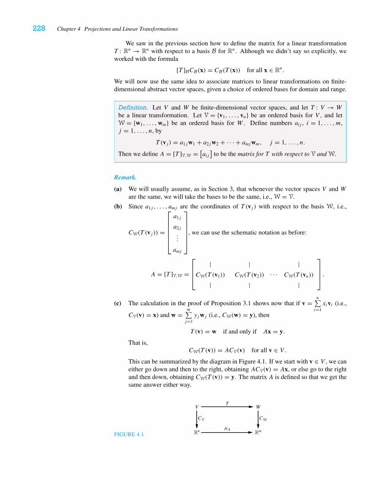
228 Chapter 4 Projections and Linear Transformations
We saw in the previous section how to define the matrix for a linear transformationT : Rn → Rn with respect to a basis B for Rn. Although we didn’t say so explicitly, weworked with the formula
[T ]BCB(x) = CB(T (x)) for all x ∈ Rn.
We will now use the same idea to associate matrices to linear transformations on finite-dimensional abstract vector spaces, given a choice of ordered bases for domain and range.
Definition. Let V and W be finite-dimensional vector spaces, and let T : V → W
be a linear transformation. Let V = {v1, . . . , vn} be an ordered basis for V , and letW = {w1, . . . ,wm} be an ordered basis for W . Define numbers aij , i = 1, . . . , m,j = 1, . . . , n, by
T (vj ) = a1jw1 + a2jw2 + · · · + amjwm, j = 1, . . . , n.
Then we define A = [T ]V,W = [aij]
to be the matrix for T with respect to V and W.
Remark.
(a) We will usually assume, as in Section 3, that whenever the vector spaces V and Ware the same, we will take the bases to be the same, i.e., W = V.
(b) Since a1j , . . . , amj are the coordinates of T (vj ) with respect to the basis W, i.e.,
CW(T (vj )) =
⎡⎢⎢⎢⎢⎢⎣
a1j
a2j
...
amj
⎤⎥⎥⎥⎥⎥⎦
, we can use the schematic notation as before:
A = [T ]V,W =
⎡⎢⎢⎣
|CW(T (v1))
|
|CW(T (v2))
|· · ·
|CW(T (vn))
|
⎤⎥⎥⎦ .
(c) The calculation in the proof of Proposition 3.1 shows now that if v =n∑i=1xivi (i.e.,
CV(v) = x) and w =m∑j=1yjwj (i.e., CW(w) = y), then
T (v) = w if and only if Ax = y.
That is,CW(T (v)) = ACV(v) for all v ∈ V.
This can be summarized by the diagram in Figure 4.1. If we start with v ∈ V , we caneither go down and then to the right, obtaining ACV(v) = Ax, or else go to the rightand then down, obtaining CW(T (v)) = y. The matrix A is defined so that we get thesame answer either way.
FIGURE 4.1
WVT
CV CW
μARn Rm
4 Linear Transformations on Abstract Vector Spaces 229
(d) What’s more, suppose U , V , and W are vector spaces with bases U, V, and W,respectively. Suppose also thatA is the matrix for a linear transformation T : V → W
with respect to V and W, and suppose thatB is the matrix for S : U → V with respectto U and V. Then, because matrix multiplication corresponds to composition of lineartransformations, AB is the matrix for T ◦S with respect to U and W.
EXAMPLE 5
Let’s return now to D : P3 → P2. Let’s choose “standard” bases for these vector spaces:V = {1, t, t2, t3} and W = {1, t, t2}. Then
D(1) = 0 = 0 · 1 + 0 · t + 0 · t2D(t) = 1 = 1 · 1 + 0 · t + 0 · t2D(t2) = 2t = 0 · 1 + 2 · t + 0 · t2D(t3) = 3t2 = 0 · 1 + 0 · t + 3 · t2.
Now—and this is always the confusing part—we must be sure to arrange these coefficientsas the columns, and not as the rows, of our matrix:
[D]V,W = A =
⎡⎢⎢⎣
0 1 0 0
0 0 2 0
0 0 0 3
⎤⎥⎥⎦ .
Let’s make sure we understand what this means. Suppose f (t) = 2 − t + 5t2 + 4t3 ∈ P3
and we wish to calculate D(f ). The coordinate vector of f with respect to the basis V is⎡⎢⎢⎢⎢⎣
2
−1
5
4
⎤⎥⎥⎥⎥⎦,
and so
A
⎡⎢⎢⎢⎢⎣
2
−1
5
4
⎤⎥⎥⎥⎥⎦
=
⎡⎢⎢⎣
0 1 0 0
0 0 2 0
0 0 0 3
⎤⎥⎥⎦
⎡⎢⎢⎢⎢⎣
2
−1
5
4
⎤⎥⎥⎥⎥⎦
=
⎡⎢⎢⎣
−1
10
12
⎤⎥⎥⎦ ,
which is the coordinate vector ofD(f ) ∈ P2 with respect to the basis W. That is,D(f ) =−1 + 10t + 12t2.
EXAMPLE 6
Define T : P3 → P4 by T (f )(t) = tf (t). Note that when we multiply a polynomial f (t)of degree ≤ 3 by t , we obtain a polynomial of degree ≤ 4. We ask the reader to check thatthis is a linear transformation. The matrix for T with respect to the bases V = {1, t, t2, t3}
230 Chapter 4 Projections and Linear Transformations
and W = {1, t, t2, t3, t4} is
A =
⎡⎢⎢⎢⎢⎢⎢⎢⎣
0 0 0 0
1 0 0 0
0 1 0 0
0 0 1 0
0 0 0 1
⎤⎥⎥⎥⎥⎥⎥⎥⎦,
as we leave it to the reader to check.
EXAMPLE 7
Define T : P3 → R2 by T (f ) =[f (0)
f (1)
]. Again we leave it to the conscientious reader to
check that this is a linear transformation. With respect to the bases V = {1, t, t2, t3} for P3
and the standard basis W = {e1, e2} for R2, the matrix for T is
A =[
1 0 0 0
1 1 1 1
].
EXAMPLE 8
Of course, if we use different bases for our vector spaces, then we will get different matricesrepresenting our linear transformation. Returning to Example 5, let’s instead use the basisV′ = {1, t − 1, (t − 1)2, (t − 1)3} for P3 and the same basis W = {1, t, t2} for P2. Then
D(1) = 0 = 0 · 1 + 0 · t + 0 · t2D(t − 1) = 1 = 1 · 1 + 0 · t + 0 · t2D((t − 1)2) = 2(t − 1) = −2 · 1 + 2 · t + 0 · t2D((t − 1)3) = 3(t − 1)2 = 3 · 1 − 6 · t + 3 · t2 .
Thus, the matrix for D with respect to the bases V′ and W is
[D]V′,W = A′ =
⎡⎢⎢⎣
0 1 −2 3
0 0 2 −6
0 0 0 3
⎤⎥⎥⎦ .
EXAMPLE 9
Fix
M =[
0 1
1 0
],
and define T : M2×2 → M2×2 by T (X) = MX. Then properties of matrix multiplicationtell us that T is a linear transformation. Using the basis V consisting of
v1 =[
1 0
0 0
], v2 =
[0 1
0 0
], v3 =
[0 0
1 0
], and v4 =
[0 0
0 1
]
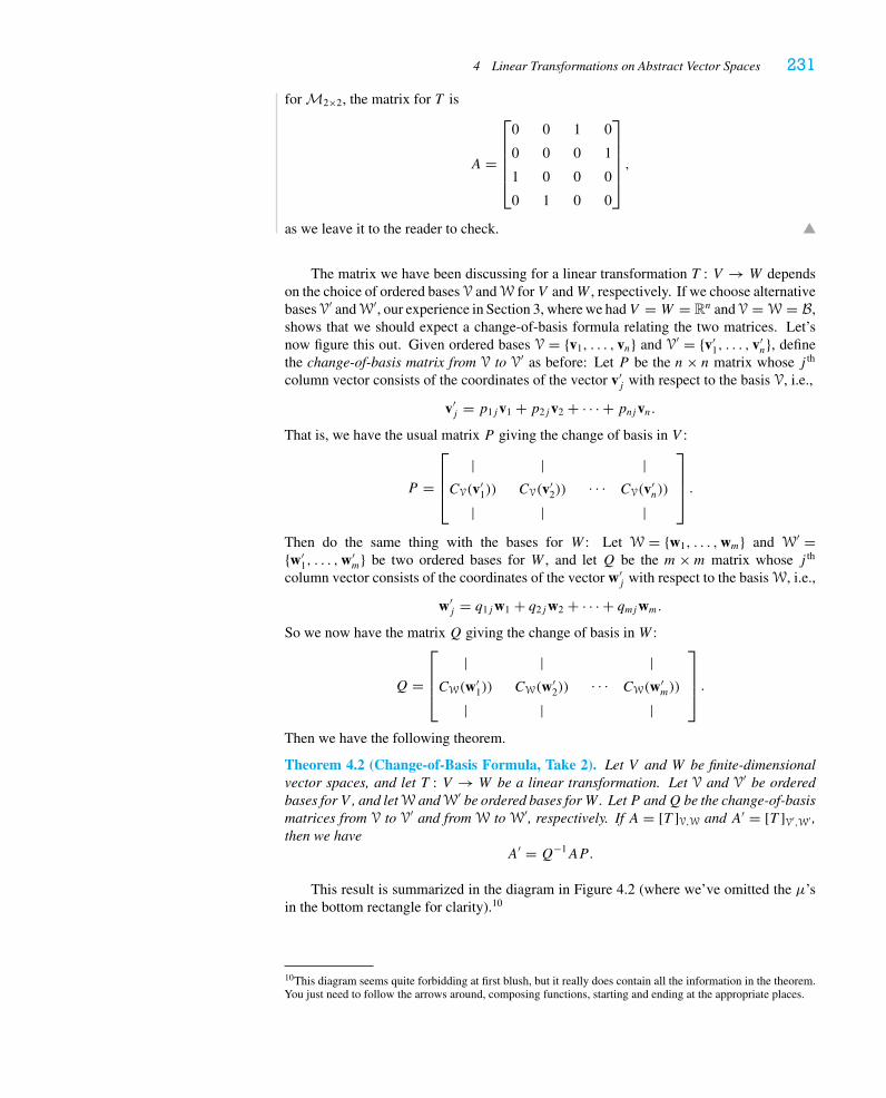
4 Linear Transformations on Abstract Vector Spaces 231
for M2×2, the matrix for T is
A =
⎡⎢⎢⎢⎢⎣
0 0 1 0
0 0 0 1
1 0 0 0
0 1 0 0
⎤⎥⎥⎥⎥⎦,
as we leave it to the reader to check.
The matrix we have been discussing for a linear transformation T : V → W dependson the choice of ordered bases V and W for V andW , respectively. If we choose alternativebases V′ and W′, our experience in Section 3, where we hadV = W = Rn and V = W = B,shows that we should expect a change-of-basis formula relating the two matrices. Let’snow figure this out. Given ordered bases V = {v1, . . . , vn} and V′ = {v′
1, . . . , v′n}, define
the change-of-basis matrix from V to V′ as before: Let P be the n× n matrix whose j th
column vector consists of the coordinates of the vector v′j with respect to the basis V, i.e.,
v′j = p1jv1 + p2jv2 + · · · + pnjvn.
That is, we have the usual matrix P giving the change of basis in V :
P =
⎡⎢⎢⎣
|CV(v′
1))
|
|CV(v′
2))
|· · ·
|CV(v′
n))
|
⎤⎥⎥⎦ .
Then do the same thing with the bases for W : Let W = {w1, . . . ,wm} and W′ ={w′
1, . . . ,w′m} be two ordered bases for W , and let Q be the m×m matrix whose j th
column vector consists of the coordinates of the vector w′j with respect to the basis W, i.e.,
w′j = q1jw1 + q2jw2 + · · · + qmjwm.
So we now have the matrixQ giving the change of basis inW :
Q =
⎡⎢⎢⎣
|CW(w′
1))
|
|CW(w′
2))
|· · ·
|CW(w′
m))
|
⎤⎥⎥⎦ .
Then we have the following theorem.
Theorem 4.2 (Change-of-Basis Formula, Take 2). Let V and W be finite-dimensionalvector spaces, and let T : V → W be a linear transformation. Let V and V′ be orderedbases for V , and let W and W′ be ordered bases forW . LetP andQ be the change-of-basismatrices from V to V′ and from W to W′, respectively. If A = [T ]V,W and A′ = [T ]V′,W′ ,then we have
A′ = Q−1AP.
This result is summarized in the diagram in Figure 4.2 (where we’ve omitted the μ’sin the bottom rectangle for clarity).10
10This diagram seems quite forbidding at first blush, but it really does contain all the information in the theorem.You just need to follow the arrows around, composing functions, starting and ending at the appropriate places.
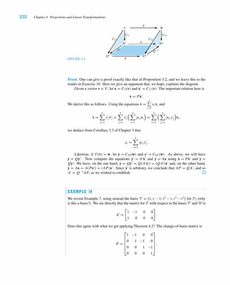
232 Chapter 4 Projections and Linear Transformations
FIGURE 4.2
WVT
Q–1P
A
RmRn
Rn Rm
CV´ CW´CV CW
A
Proof. One can give a proof exactly like that of Proposition 3.2, and we leave this to thereader in Exercise 10. Here we give an argument that, we hope, explains the diagram.
Given a vector v ∈ V , let x = CV(v) and x′ = CV′(v). The important relation here is
x = Px′.
We derive this as follows. Using the equations v =n∑i=1xivi and
v =n∑j=1
x ′jv
′j =
n∑j=1
x ′j
( n∑i=1
pijvi)
=n∑i=1
( n∑j=1
pijx′j
)vi ,
we deduce from Corollary 3.3 of Chapter 3 that
xi =n∑j=1
pijx′j .
Likewise, if T (v) = w, let y = CW(w) and y′ = CW′(w). As above, we will havey = Qy′. Now compare the equations y′ = A′x′ and y = Ax using x = Px′ and y =Qy′: We have, on the one hand, y = Qy′ = Q(A′x′) = (QA′)x′ and, on the other hand,y = Ax = A(Px′) = (AP )x′. Since x′ is arbitrary, we conclude that AP = QA′, and soA′ = Q−1AP , as we wished to establish.
EXAMPLE 10
We revisit Example 7, using instead the basis V′ = {1, t − 1, t2 − t, t3 − t2} for P3 (whyis this a basis?). We see directly that the matrix for T with respect to the bases V′ and W is
A′ =[
1 −1 0 0
1 0 0 0
].
Does this agree with what we get applying Theorem 4.2? The change-of-basis matrix is
P =
⎡⎢⎢⎢⎢⎣
1 −1 0 0
0 1 −1 0
0 0 1 −1
0 0 0 1
⎤⎥⎥⎥⎥⎦,
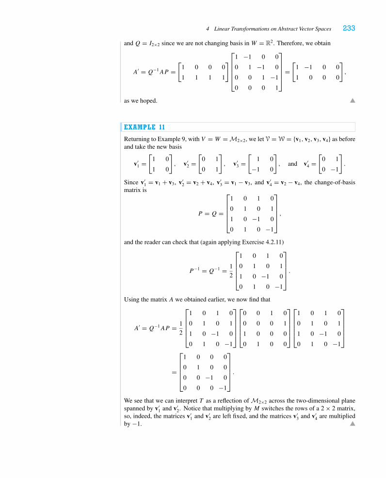
4 Linear Transformations on Abstract Vector Spaces 233
andQ = I2×2 since we are not changing basis inW = R2. Therefore, we obtain
A′ = Q−1AP =[
1 0 0 0
1 1 1 1
]⎡⎢⎢⎢⎢⎣
1 −1 0 0
0 1 −1 0
0 0 1 −1
0 0 0 1
⎤⎥⎥⎥⎥⎦
=[
1 −1 0 0
1 0 0 0
],
as we hoped.
EXAMPLE 11
Returning to Example 9, with V = W = M2×2, we let V = W = {v1, v2, v3, v4} as beforeand take the new basis
v′1 =
[1 0
1 0
], v′
2 =[
0 1
0 1
], v′
3 =[
1 0
−1 0
], and v′
4 =[
0 1
0 −1
].
Since v′1 = v1 + v3, v′
2 = v2 + v4, v′3 = v1 − v3, and v′
4 = v2 − v4, the change-of-basismatrix is
P = Q =
⎡⎢⎢⎢⎢⎣
1 0 1 0
0 1 0 1
1 0 −1 0
0 1 0 −1
⎤⎥⎥⎥⎥⎦,
and the reader can check that (again applying Exercise 4.2.11)
P−1 = Q−1 = 1
2
⎡⎢⎢⎢⎢⎣
1 0 1 0
0 1 0 1
1 0 −1 0
0 1 0 −1
⎤⎥⎥⎥⎥⎦.
Using the matrix A we obtained earlier, we now find that
A′ = Q−1AP = 1
2
⎡⎢⎢⎢⎢⎣
1 0 1 0
0 1 0 1
1 0 −1 0
0 1 0 −1
⎤⎥⎥⎥⎥⎦
⎡⎢⎢⎢⎢⎣
0 0 1 0
0 0 0 1
1 0 0 0
0 1 0 0
⎤⎥⎥⎥⎥⎦
⎡⎢⎢⎢⎢⎣
1 0 1 0
0 1 0 1
1 0 −1 0
0 1 0 −1
⎤⎥⎥⎥⎥⎦
=
⎡⎢⎢⎢⎢⎣
1 0 0 0
0 1 0 0
0 0 −1 0
0 0 0 −1
⎤⎥⎥⎥⎥⎦.
We see that we can interpret T as a reflection of M2×2 across the two-dimensional planespanned by v′
1 and v′2. Notice that multiplying by M switches the rows of a 2 × 2 matrix,
so, indeed, the matrices v′1 and v′
2 are left fixed, and the matrices v′3 and v′
4 are multipliedby −1.
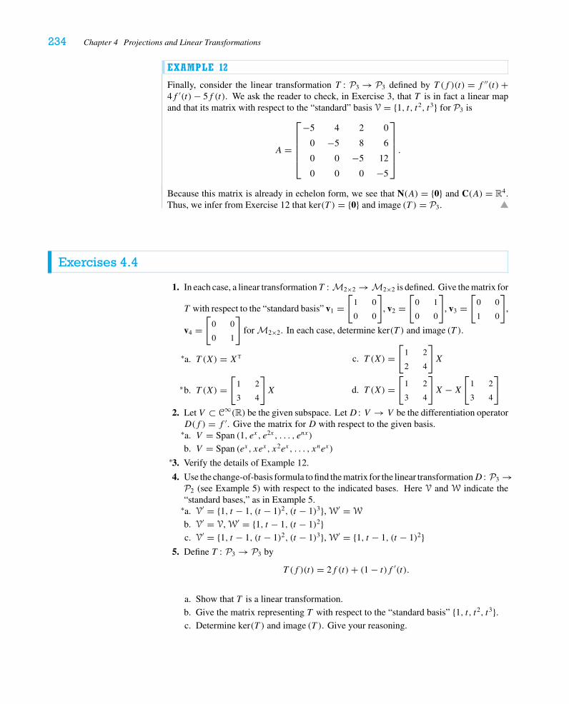
234 Chapter 4 Projections and Linear Transformations
EXAMPLE 12
Finally, consider the linear transformation T : P3 → P3 defined by T (f )(t) = f ′′(t)+4f ′(t)− 5f (t). We ask the reader to check, in Exercise 3, that T is in fact a linear mapand that its matrix with respect to the “standard” basis V = {1, t, t2, t3} for P3 is
A =
⎡⎢⎢⎢⎢⎣
−5 4 2 0
0 −5 8 6
0 0 −5 12
0 0 0 −5
⎤⎥⎥⎥⎥⎦.
Because this matrix is already in echelon form, we see that N(A) = {0} and C(A) = R4.Thus, we infer from Exercise 12 that ker(T ) = {0} and image (T ) = P3.
Exercises 4.4
1. In each case, a linear transformationT : M2×2 → M2×2 is defined. Give the matrix for
T with respect to the “standard basis” v1 =[
1 0
0 0
], v2 =
[0 1
0 0
], v3 =
[0 0
1 0
],
v4 =[
0 0
0 1
]for M2×2. In each case, determine ker(T ) and image (T ).
a.∗ T (X) = XT
b.∗ T (X) =[
1 2
3 4
]X
c. T (X) =[
1 2
2 4
]X
d. T (X) =[
1 2
3 4
]X −X
[1 2
3 4
]
2. Let V ⊂ C∞(R) be the given subspace. LetD : V → V be the differentiation operatorD(f ) = f ′. Give the matrix for D with respect to the given basis.a.∗ V = Span (1, ex, e2x, . . . , enx)
b. V = Span (ex, xex, x2ex, . . . , xnex)
3.∗ Verify the details of Example 12.
4. Use the change-of-basis formula to find the matrix for the linear transformationD : P3 →P2 (see Example 5) with respect to the indicated bases. Here V and W indicate the“standard bases,” as in Example 5.a.∗ V′ = {1, t − 1, (t − 1)2, (t − 1)3}, W′ = W
b. V′ = V, W′ = {1, t − 1, (t − 1)2}c. V′ = {1, t − 1, (t − 1)2, (t − 1)3}, W′ = {1, t − 1, (t − 1)2}
5. Define T : P3 → P3 by
T (f )(t) = 2f (t)+ (1 − t)f ′(t).
a. Show that T is a linear transformation.
b. Give the matrix representing T with respect to the “standard basis” {1, t, t2, t3}.c. Determine ker(T ) and image (T ). Give your reasoning.
4 Linear Transformations on Abstract Vector Spaces 235
d. Let g(t) = 1 + 2t . Use your answer to part b to find a solution of the differentialequation T (f ) = g.
e. What are all the solutions of T (f ) = g?
6. Consider the differentiation operator D : C1(R) → C0(R) (or Pk → Pk−1, if youprefer).a. Show that ker(D) = {constant functions}.b. Give the interpretation of Theorem 5.3 of Chapter 1 familiar to all students of
calculus.
7. Define M : P → P by M(f )(t) = tf (t), and let D : P → P be the differentiationoperator, as usual.a. Calculate D◦M −M◦D.
b. Check your result of part a with matrices if you consider the transformation mappingthe finite-dimensional subspace P3 to P3. (Remark: You will need to use thematrices for both D : P3 → P2 and D : P4 → P3, as well as the matrices for bothM : P2 → P3 andM : P3 → P4.)
c. Show that there can be no linear transformations S : V → V and T : V → V on afinite-dimensional vector space V with the property that S◦T − T ◦S = I . (Hint:See Exercise 3.6.9.) Why does this not contradict the result of part b?
8. Let V andW be vector spaces, and let T : V → W be a linear transformation.a.∗ Show that T maps the line through u and v to the line through T (u) and T (v). What
does this mean if T (u) = T (v)?b. Show that T maps parallel lines to parallel lines.
9. a. Consider the identity transformation Id : Rn → Rn. Using the basis V in the domainand the basis V′ in the range, show that the matrix [Id]V,V′ is the inverse of thechange-of-basis matrix P .
b. Use this observation to give another derivation of the change-of-basis formula.
10. Give a proof of Theorem 4.2 modeled on the proof of Proposition 3.2.
11. Let V andW be vector spaces (not necessarily finite-dimensional), and let T : V → W
be a linear transformation. Check that ker(T ) ⊂ V and image (T ) ⊂ W are subspaces.
12. Suppose V = {v1, . . . , vn} is an ordered basis for V , W = {w1, . . . ,wm} is an orderedbasis forW , and A is the matrix for the linear transformation T : V → W with respectto these bases.a. Check that x ∈ N(A) ⇐⇒ x1v1 + · · · + xnvn ∈ ker(T ).
b. Check that y ∈ C(A) ⇐⇒ y1w1 + · · · + ymwm ∈ image (T ).
13. Prove that if a linear transformation T : V → W is an isomorphism, then there isa linear transformation T −1 : W → V satisfying (T −1◦T )(v) = v for all v ∈ V and(T ◦T −1)(w) = w for all w ∈ W .
14. Decide whether each of the following functions T is a linear transformation. If not,explain why. If so, give ker(T ) and image (T ).a.∗ T : Rn → R, T (x) = ‖x‖b.∗ T : P3 → R, T (f ) = ∫ 1
0 f (t) dt
c. T : Mm×n → Mn×m, T (X) = XT
d.∗ T : P → P , T (f )(t) = ∫ t0 f (s) dse. T : C0(R) → C1(R), T (f )(t) = ∫ t0 f (s) ds
15. Let I = [0, 1], and let M : C0(I) → C0(I) be given by M(f )(t) = tf (t). Determineker(T ) and image (T ).
236 Chapter 4 Projections and Linear Transformations
16. Let V be a finite-dimensional vector space, letW be a vector space, and let T : V → W
be a linear transformation. Give a matrix-free proof that dim(ker T )+ dim(image T ) =dim V , as follows.a. Let {v1, . . . , vk} be a basis for ker T , and (following Exercise 3.4.17) extend to
obtain a basis {v1, . . . , vk, vk+1, . . . , vn} for V . Show that {T (vk+1), . . . , T (vn)}gives a basis for image (T ).
b. Conclude the desired result. Explain why this is a restatement of Corollary 4.7 ofChapter 3 whenW is finite-dimensional.
17. Suppose T : V → W is an isomorphism and dim V = n. Prove that dimW = n.
18. a. Suppose T : V → W is a linear transformation. Suppose {v1, . . . , vk} ⊂ V is lin-early dependent. Prove that {T (v1), . . . , T (vk)} ⊂ W is linearly dependent.
b. Suppose T : V → V is a linear transformation and V is finite-dimensional. Sup-pose image (T ) = V . Prove that if {v1, . . . , vk} ⊂ V is linearly independent, then{T (v1), . . . , T (vk)} is linearly independent. (Hint: Use Exercise 12 or Exercise16.)
19. Let V and W be subspaces of Rn with V ∩W = {0}. Let S = projV and T = projW .Show that S◦T = T ◦S if and only if V and W are orthogonal subspaces. (They neednot be orthogonal complements, however.)
20. Suppose V is a vector space and T : V → V is a linear transformation. Supposev1, v2, v3 ∈ V are nonzero vectors satisfying
T (v1) = v1
T (v2) = 2v2
T (v3) = −v3.
Prove that {v1, v2, v3} is linearly independent.
21. Let V be a vector space.a. Let V ∗ denote the set of all linear transformations from V to R. Show that V ∗ is a
vector space.
b. Suppose {v1, . . . , vn} is a basis for V . For i = 1, . . . , n, define fi ∈ V ∗ by
fi (a1v1 + a2v2 + · · · + anvn) = ai.
Prove that {f1, . . . , fn} gives a basis for V ∗.
c. Deduce that whenever V is finite-dimensional, dim V ∗ = dim V .
22. Let t1, . . . , tk+1 be distinct real numbers. Define a linear transformationT : Pk → Rk+1
by
T (f ) =
⎡⎢⎢⎢⎢⎢⎣
f (t1)
f (t2)
...
f (tk+1)
⎤⎥⎥⎥⎥⎥⎦.
a. Prove that ker(T ) = {0}.b. Show that the matrix for T with respect to the “standard bases” for Pk and Rk+1 is
the matrix A on p. 185.
c. Deduce that the matrix A on p. 185 is nonsingular. (See Exercise 12.)
d. Explain the origins of the inner product on Pk defined in Example 10(b) in Section6 of Chapter 3.
Historical Notes 237
23. Suppose T : Rn → Rn has the following properties:
(i) T (0) = 0;
(ii) T preserves distance (i.e., ‖T (x)− T (y)‖ = ‖x − y‖ for all x, y ∈ Rn).
a. Prove that T (x) · T (y) = x · y for all x, y ∈ Rn.
b. If {e1, . . . , en} is the standard basis, letT (ei ) = vi . Prove thatT( n∑i=1xiei) =
n∑i=1xivi .
c. Deduce from part b that T is a linear transformation.
d. Prove that the standard matrix for T is orthogonal.
24. (See the discussion on p. 167 and Exercise 3.4.25.) Let A be an n× n matrix. Provethat the functions μA : R(A) → C(A) and μAT : C(A) → R(A) are inverse functionsif and only if A = QP , where P is a projection matrix andQ is orthogonal.
HISTORICAL NOTESCarl Friedrich Gauss (1777–1855) invented the method of least squares while he was study-ing the orbits of asteroids. In 1801 he successfully predicted the orbit of Ceres, an asteroiddiscovered by the Italian astronomer G. Piazzi on the first day of that year. The work was soimpressive that the German astronomer Wilhelm Olbers asked him to apply his methods tostudy the second known asteroid, Pallas, which Olbers had discovered in 1802. In a paperof 1809, Gauss summarized his work on Pallas. His calculations had led him to an incon-sistent linear system in six variables, which therefore required a least-squares approach.In the same paper he also used the techniques of what we now call Gaussian elimination.Adrien-Marie Legendre (1752–1833) actually published the least squares method first, in1806, in a book describing methods for determining the orbits of comets. Gauss claimedpriority in his book, and it is now generally accepted that he was the first to design and usethe method.
The uses of orthogonality and orthogonal projections go far beyond the statistical anal-ysis of data. Jean Baptiste Joseph Fourier (1768–1830) was a great French mathematicianwho focused much of his attention on understanding and modeling physical phenomenasuch as heat transfer and vibration. His work led to what is now called Fourier series and theapproach to problem solving called Fourier analysis. Fourier was a mathematical prodigyand studied at the École Royale Militaire in his hometown of Auxerre. A short time afterleaving school, he applied to enter the artillery or the engineers, but was denied. He thendecided, at the age of nineteen, to join an abbey to study for the priesthood. He nevertook his religious vows; instead, he was offered a professorship at the École Militaire, andmathematics became his life’s work. He was imprisoned during the Reign of Terror in 1794and may have come close to being guillotined. He accepted a job at the École Normale inParis, starting in 1795, and soon thereafter was offered the chair of analysis at the ÉcolePolytechnique. He accompanied Napoleon as scientific adviser to Egypt in 1798 and wasrewarded by being appointed governor of lower Egypt. When he returned to Paris in 1801,he was appointed prefect of the Department of Isère.
During his time in Grenoble, Fourier developed his theory of heat, completing hismemoir On the Propagation of Heat in Solid Bodies (1807). Fourier’s ideas were metwith a cold reception when he proposed them in the early nineteenth century, but now histechniques are indispensable in fields such as electrical engineering. The fundamental ideabehind Fourier analysis is that many functions can be approximated by linear combinationsof the functions 1, cos nx, and sin nx, as n ranges over all positive integers. These functionsare orthogonal in the vector space of continuous functions on the interval [0, 2π ] endowed

238 Chapter 4 Projections and Linear Transformations
with the inner product described in Example 10(c) in Section 6 of Chapter 3. Thus, thebasic idea of Fourier analysis is that continuous functions should be well approximatedby their projections onto (finite-dimensional) spans of these orthogonal functions. Otherclasses of orthogonal functions have been studied over the years and applied to the theory ofdifferential equations by mathematicians such as Legendre, Charles Hermite (1822–1901),Pafnuty Lvovich Chebyshev (1821–1894), and Edmond Nicolas Laguerre (1834–1886).Many of these ideas have also played a significant role in the modern theory of interpolationand numerical integration.
239
C H A P T E R 5DETERMINANTS
To each square matrix we associate a number, called its determinant. For us, that number willprovide a convenient computational criterion for determining whether a matrix is singular.We will use this criterion in Chapter 6. The determinant also has a geometric interpretationin terms of area and volume. Although this interpretation is not necessary for our laterwork, we find it such a beautiful example of the interplay between algebra and geometrythat we could not resist telling at least part of this story. Those who study multivariablecalculus will recognize the determinant when it appears in the change-of-variables formulafor integrals.
1 Properties of Determinants
In Section 3 of Chapter 2 we saw that a 2 × 2 matrix A =[a b
c d
]is nonsingular if and
only if the quantity ad − bc is nonzero. Here we give this quantity a name, the determinantof A, denoted detA; i.e., detA = ad − bc. We will explore the geometric interpretationof the determinant in Section 3, but for now we want to figure out how this idea shouldgeneralize to n× n matrices. To do this, we will study the effect of row operations on thedeterminant. If we switch the two rows, the determinant changes sign. If we multiply oneof the rows by a scalar, the determinant multiplies by that same factor. Slightly less obviousis the observation that if we do a row operation of type (iii)—adding a multiple of one rowto the other—then the determinant does not change: For any scalar k, consider that
det
[a b
c + ka d + kb
]= a(d + kb)− b(c + ka) = ad − bc = det
[a b
c d
].
Now let’s reverse this reasoning. Starting with these three properties and the re-quirement that the determinant of the identity matrix be 1, can we derive the formula
detA = ad − bc? LetA =[a b
c d
]and assume that a �= 0. First we add −c/a times the
first row to the second: [a b
c d
]�[a b
0 d − bca
].
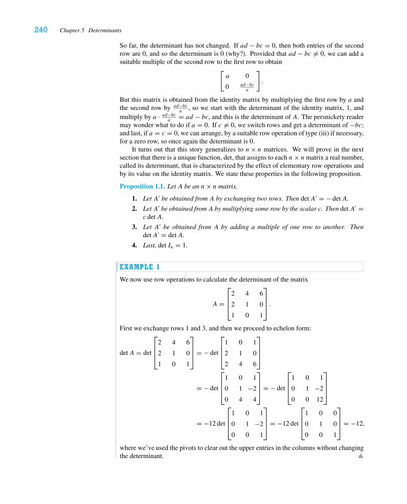
240 Chapter 5 Determinants
So far, the determinant has not changed. If ad − bc = 0, then both entries of the secondrow are 0, and so the determinant is 0 (why?). Provided that ad − bc �= 0, we can add asuitable multiple of the second row to the first row to obtain
[a 0
0 ad−bca
].
But this matrix is obtained from the identity matrix by multiplying the first row by a andthe second row by ad−bc
a, so we start with the determinant of the identity matrix, 1, and
multiply by a · ad−bca
= ad − bc, and this is the determinant of A. The persnickety readermay wonder what to do if a = 0. If c �= 0, we switch rows and get a determinant of −bc;and last, if a = c = 0, we can arrange, by a suitable row operation of type (iii) if necessary,for a zero row, so once again the determinant is 0.
It turns out that this story generalizes to n× n matrices. We will prove in the nextsection that there is a unique function, det, that assigns to each n× nmatrix a real number,called its determinant, that is characterized by the effect of elementary row operations andby its value on the identity matrix. We state these properties in the following proposition.
Proposition 1.1. Let A be an n× n matrix.
1. Let A′ be obtained from A by exchanging two rows. Then detA′ = − detA.
2. LetA′ be obtained fromA by multiplying some row by the scalar c. Then detA′ =c detA.
3. Let A′ be obtained from A by adding a multiple of one row to another. ThendetA′ = detA.
4. Last, det In = 1.
EXAMPLE 1
We now use row operations to calculate the determinant of the matrix
A =
⎡⎢⎢⎣
2 4 6
2 1 0
1 0 1
⎤⎥⎥⎦ .
First we exchange rows 1 and 3, and then we proceed to echelon form:
detA = det
⎡⎢⎢⎣
2 4 6
2 1 0
1 0 1
⎤⎥⎥⎦ = − det
⎡⎢⎢⎣
1 0 1
2 1 0
2 4 6
⎤⎥⎥⎦
= − det
⎡⎢⎢⎣
1 0 1
0 1 −2
0 4 4
⎤⎥⎥⎦ = − det
⎡⎢⎢⎣
1 0 1
0 1 −2
0 0 12
⎤⎥⎥⎦
= −12 det
⎡⎢⎢⎣
1 0 1
0 1 −2
0 0 1
⎤⎥⎥⎦ = −12 det
⎡⎢⎢⎣
1 0 0
0 1 0
0 0 1
⎤⎥⎥⎦ = −12,
where we’ve used the pivots to clear out the upper entries in the columns without changingthe determinant.
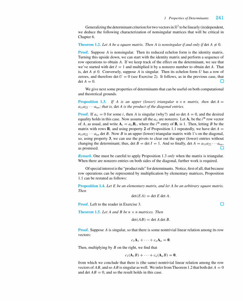
1 Properties of Determinants 241
Generalizing the determinant criterion for two vectors in R2 to be linearly (in)dependent,we deduce the following characterization of nonsingular matrices that will be critical inChapter 6.
Theorem 1.2. Let A be a square matrix. Then A is nonsingular if and only if detA �= 0.
Proof. Suppose A is nonsingular. Then its reduced echelon form is the identity matrix.Turning this upside down, we can start with the identity matrix and perform a sequence ofrow operations to obtain A. If we keep track of the effect on the determinant, we see thatwe’ve started with det I = 1 and multiplied it by a nonzero number to obtain detA. Thatis, detA �= 0. Conversely, suppose A is singular. Then its echelon form U has a row ofzeroes, and therefore detU = 0 (see Exercise 2). It follows, as in the previous case, thatdetA = 0.
We give next some properties of determinants that can be useful on both computationaland theoretical grounds.
Proposition 1.3. If A is an upper (lower) triangular n× n matrix, then detA =a11a22 · · · ann; that is, detA is the product of the diagonal entries.
Proof. If aii = 0 for some i, then A is singular (why?) and so detA = 0, and the desiredequality holds in this case. Now assume all the aii are nonzero. Let Ai be the i th row vectorof A, as usual, and write Ai = aiiBi , where the i th entry of Bi is 1. Then, letting B be thematrix with rows Bi and using property 2 of Proposition 1.1 repeatedly, we have detA =a11a22 · · · ann detB. Now B is an upper (lower) triangular matrix with 1’s on the diagonal,so, using property 3, we can use the pivots to clear out the upper (lower) entries withoutchanging the determinant; thus, detB = det I = 1. And so finally, detA = a11a22 · · · ann,as promised.
Remark. One must be careful to apply Proposition 1.3 only when the matrix is triangular.When there are nonzero entries on both sides of the diagonal, further work is required.
Of special interest is the “product rule” for determinants. Notice, first of all, that becauserow operations can be represented by multiplication by elementary matrices, Proposition1.1 can be restated as follows:
Proposition 1.4. Let E be an elementary matrix, and let A be an arbitrary square matrix.Then
det(EA) = detE detA.
Proof. Left to the reader in Exercise 3.
Theorem 1.5. Let A and B be n× n matrices. Then
det(AB) = detA detB.
Proof. Suppose A is singular, so that there is some nontrivial linear relation among its rowvectors:
c1A1 + · · · + cnAn = 0.
Then, multiplying by B on the right, we find that
c1(A1B)+ · · · + cn(AnB) = 0,
from which we conclude that there is (the same) nontrivial linear relation among the rowvectors ofAB, and soAB is singular as well. We infer from Theorem 1.2 that both detA = 0and detAB = 0, and so the result holds in this case.
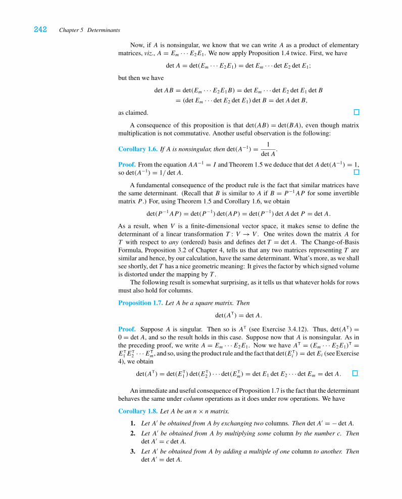
242 Chapter 5 Determinants
Now, if A is nonsingular, we know that we can write A as a product of elementarymatrices, viz., A = Em · · ·E2E1. We now apply Proposition 1.4 twice. First, we have
detA = det(Em · · ·E2E1) = detEm · · · detE2 detE1;but then we have
detAB = det(Em · · ·E2E1B) = detEm · · · detE2 detE1 detB
= (detEm · · · detE2 detE1) detB = detA detB,
as claimed.
A consequence of this proposition is that det(AB) = det(BA), even though matrixmultiplication is not commutative. Another useful observation is the following:
Corollary 1.6. If A is nonsingular, then det(A−1) = 1
detA.
Proof. From the equationAA−1 = I and Theorem 1.5 we deduce that detA det(A−1) = 1,so det(A−1) = 1/ detA.
A fundamental consequence of the product rule is the fact that similar matrices havethe same determinant. (Recall that B is similar to A if B = P−1AP for some invertiblematrix P .) For, using Theorem 1.5 and Corollary 1.6, we obtain
det(P−1AP) = det(P−1) det(AP ) = det(P−1) detA det P = detA.
As a result, when V is a finite-dimensional vector space, it makes sense to define thedeterminant of a linear transformation T : V → V . One writes down the matrix A forT with respect to any (ordered) basis and defines det T = detA. The Change-of-BasisFormula, Proposition 3.2 of Chapter 4, tells us that any two matrices representing T aresimilar and hence, by our calculation, have the same determinant. What’s more, as we shallsee shortly, det T has a nice geometric meaning: It gives the factor by which signed volumeis distorted under the mapping by T .
The following result is somewhat surprising, as it tells us that whatever holds for rowsmust also hold for columns.
Proposition 1.7. Let A be a square matrix. Then
det(AT) = detA.
Proof. Suppose A is singular. Then so is AT (see Exercise 3.4.12). Thus, det(AT) =0 = detA, and so the result holds in this case. Suppose now that A is nonsingular. As inthe preceding proof, we write A = Em · · ·E2E1. Now we have AT = (Em · · ·E2E1)
T =ET
1ET2 · · ·ET
m, and so, using the product rule and the fact that det(ETi ) = detEi (see Exercise
4), we obtain
det(AT) = det(ET1 ) det(ET
2 ) · · · det(ETm) = detE1 detE2 · · · detEm = detA.
An immediate and useful consequence of Proposition 1.7 is the fact that the determinantbehaves the same under column operations as it does under row operations. We have
Corollary 1.8. Let A be an n× n matrix.
1. Let A′ be obtained from A by exchanging two columns. Then detA′ = − detA.
2. Let A′ be obtained from A by multiplying some column by the number c. ThendetA′ = c detA.
3. Let A′ be obtained from A by adding a multiple of one column to another. ThendetA′ = detA.
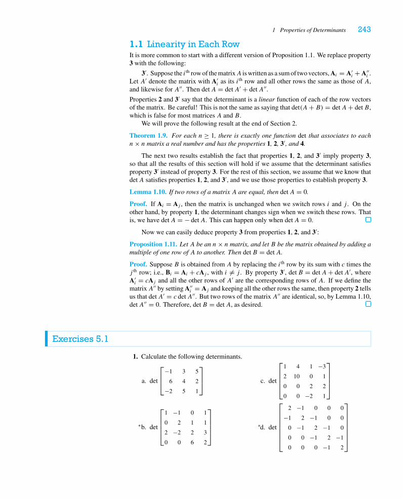
1 Properties of Determinants 243
1.1 Linearity in Each RowIt is more common to start with a different version of Proposition 1.1. We replace property3 with the following:
3′. Suppose the i th row of the matrixA is written as a sum of two vectors, Ai = A′i + A′′
i .Let A′ denote the matrix with A′
i as its i th row and all other rows the same as those of A,and likewise for A′′. Then detA = detA′ + detA′′.Properties 2 and 3′ say that the determinant is a linear function of each of the row vectorsof the matrix. Be careful! This is not the same as saying that det(A+ B) = detA+ detB,which is false for most matrices A and B.
We will prove the following result at the end of Section 2.
Theorem 1.9. For each n ≥ 1, there is exactly one function det that associates to eachn× n matrix a real number and has the properties 1, 2, 3′, and 4.
The next two results establish the fact that properties 1, 2, and 3′ imply property 3,so that all the results of this section will hold if we assume that the determinant satisfiesproperty 3′ instead of property 3. For the rest of this section, we assume that we know thatdetA satisfies properties 1, 2, and 3′, and we use those properties to establish property 3.
Lemma 1.10. If two rows of a matrix A are equal, then detA = 0.
Proof. If Ai = Aj , then the matrix is unchanged when we switch rows i and j . On theother hand, by property 1, the determinant changes sign when we switch these rows. Thatis, we have detA = − detA. This can happen only when detA = 0.
Now we can easily deduce property 3 from properties 1, 2, and 3′:
Proposition 1.11. Let A be an n× n matrix, and let B be the matrix obtained by adding amultiple of one row of A to another. Then detB = detA.
Proof. Suppose B is obtained from A by replacing the i th row by its sum with c times thej th row; i.e., Bi = Ai + cAj , with i �= j . By property 3′, detB = detA+ detA′, whereA′i = cAj and all the other rows of A′ are the corresponding rows of A. If we define the
matrixA′′ by setting A′′i = Aj and keeping all the other rows the same, then property 2 tells
us that detA′ = c detA′′. But two rows of the matrix A′′ are identical, so, by Lemma 1.10,detA′′ = 0. Therefore, detB = detA, as desired.
Exercises 5.1
1. Calculate the following determinants.
a. det
⎡⎢⎣
−1 3 5
6 4 2
−2 5 1
⎤⎥⎦
b.∗ det
⎡⎢⎢⎢⎣
1 −1 0 1
0 2 1 1
2 −2 2 3
0 0 6 2
⎤⎥⎥⎥⎦
c. det
⎡⎢⎢⎢⎣
1 4 1 −3
2 10 0 1
0 0 2 2
0 0 −2 1
⎤⎥⎥⎥⎦
d.∗ det
⎡⎢⎢⎢⎢⎢⎢⎣
2 −1 0 0 0
−1 2 −1 0 0
0 −1 2 −1 0
0 0 −1 2 −1
0 0 0 −1 2
⎤⎥⎥⎥⎥⎥⎥⎦
244 Chapter 5 Determinants
2. Suppose one row of the n× nmatrixA consists only of 0 entries, i.e., Ai = 0 for somei. Use the properties of determinants to show that detA = 0.
3. Prove Proposition 1.4.
4.� Without using Proposition 1.7, show that for any elementary matrix E, we havedetET = detE. (Hint: Consider each of the three types of elementary matrices.)
5. Let A be an n× n matrix and let c be a scalar. Show that det(cA) = cn detA.
6. Given that 1898, 3471, 7215, and 8164 are all divisible by 13, use properties of deter-minants to show that
det
⎡⎢⎢⎢⎢⎣
1 8 9 8
3 4 7 1
7 2 1 5
8 1 6 4
⎤⎥⎥⎥⎥⎦
is divisible by 13. (Hint: Use Corollary 1.8. You may also use the result of Exercise5.2.6—the determinant of a matrix with integer entries is an integer.)
7.� Let A be an n× n matrix. Show that
det
⎡⎢⎢⎢⎢⎢⎣
1 0 · · · 0
0... A
0
⎤⎥⎥⎥⎥⎥⎦
= detA.
8. a. Show that
det
⎡⎢⎢⎣
1 1 1
b c d
b2 c2 d2
⎤⎥⎥⎦ = (c − b)(d − b)(d − c).
b. Show that
det
⎡⎢⎢⎢⎢⎣
1 1 1 1
a b c d
a2 b2 c2 d2
a3 b3 c3 d3
⎤⎥⎥⎥⎥⎦
= (b − a)(c − a)(d − a)(c − b)(d − b)(d − c).
c.∗ In general, evaluate (with proof)
det
⎡⎢⎢⎢⎢⎢⎣
1 t1 t21 . . . t k1
1 t2 t22 . . . t k2...
......
. . ....
1 tk+1 t2k+1 . . . t kk+1
⎤⎥⎥⎥⎥⎥⎦.
(See Exercises 3.6.12 and 4.4.22.)
2 Cofactors and Cramer’s Rule 245
9. Generalizing Exercise 7, we have:a.� Suppose A ∈ Mk×k , B ∈ Mk×�, and D ∈ M�×�. Prove that
det
[A B
O D
]= detA detD.
b. Suppose now that A, B, and D are as in part a and C ∈ M�×k . Prove that if A isinvertible, then
det
[A B
C D
]= detA det(D − CA−1B).
c. If we assume, moreover, that k = � and AC = CA, then deduce that
det
[A B
C D
]= det(AD − CB).
d. Give an example to show that the result of part c needn’t hold whenA and C do notcommute.
10.∗ Suppose A is an orthogonal n× n matrix. (Recall that this means that ATA = In.)What are the possible values of detA?
11. SupposeA is a skew-symmetric n× nmatrix. (Recall that this means thatAT = −A.)Show that when n is odd, detA = 0. Give an example to show that this needn’t be truewhen n is even. (Hint: Use Exercise 5.)
12. Prove directly that properties 1, 2, and 3 imply property 3′ for the last row.a. Do the case of 2 × 2 matrices first. Suppose first that {A1,A′
2} is linearly dependent;show that in this case, detA = detA′′. Next, deduce the result when {A1,A′
2} islinearly independent by writing A′′
2 as a linear combination of A1 and A′2.
b. Generalize this argument to n× n matrices. Consider first the case that {A1, . . . ,
An−1,A′n} is linearly dependent, then the case that {A1, . . . ,An−1,A′
n} is linearlyindependent.
13. Using Proposition 1.4, prove the uniqueness statement in Theorem 1.9. That is, provethat the determinant function is uniquely determined by the properties 1, 2, 3′, and 4.(Hint: Mimic the proof of Theorem 1.5. It might be helpful to consider two functionsdet and det that have these properties and to show that det(A) = det(A) for everysquare matrix A.)
2 Cofactors and Cramer’s RuleWe began this chapter with a succinct formula for the determinant of a 2 × 2 matrix:
det
[a11 a12
a21 a22
]= a11a22 − a12a21,
and we showed that this function on M2×2 satisfies the properties listed in Proposition
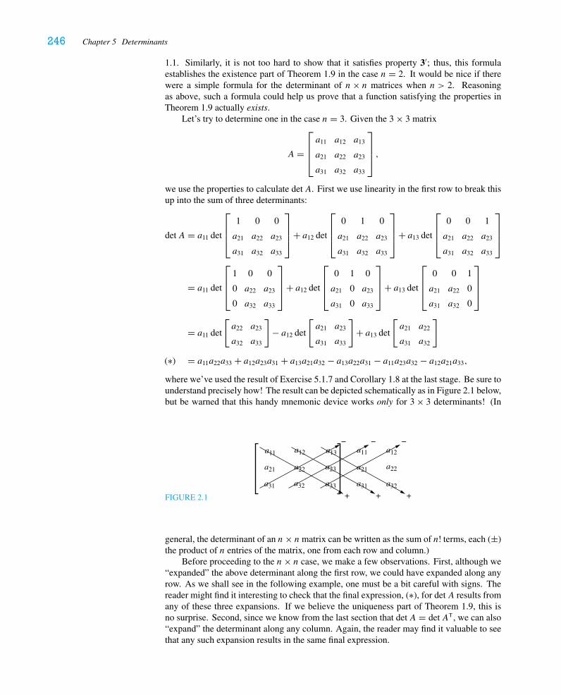
246 Chapter 5 Determinants
1.1. Similarly, it is not too hard to show that it satisfies property 3′; thus, this formulaestablishes the existence part of Theorem 1.9 in the case n = 2. It would be nice if therewere a simple formula for the determinant of n× n matrices when n > 2. Reasoningas above, such a formula could help us prove that a function satisfying the properties inTheorem 1.9 actually exists.
Let’s try to determine one in the case n = 3. Given the 3 × 3 matrix
A =
⎡⎢⎢⎣a11 a12 a13
a21 a22 a23
a31 a32 a33
⎤⎥⎥⎦ ,
we use the properties to calculate detA. First we use linearity in the first row to break thisup into the sum of three determinants:
detA = a11 det
⎡⎢⎢⎣
1 0 0
a21 a22 a23
a31 a32 a33
⎤⎥⎥⎦+ a12 det
⎡⎢⎢⎣
0 1 0
a21 a22 a23
a31 a32 a33
⎤⎥⎥⎦+ a13 det
⎡⎢⎢⎣
0 0 1
a21 a22 a23
a31 a32 a33
⎤⎥⎥⎦
= a11 det
⎡⎢⎢⎣
1 0 0
0 a22 a23
0 a32 a33
⎤⎥⎥⎦+ a12 det
⎡⎢⎢⎣
0 1 0
a21 0 a23
a31 0 a33
⎤⎥⎥⎦+ a13 det
⎡⎢⎢⎣
0 0 1
a21 a22 0
a31 a32 0
⎤⎥⎥⎦
= a11 det
[a22 a23
a32 a33
]− a12 det
[a21 a23
a31 a33
]+ a13 det
[a21 a22
a31 a32
]
(∗) = a11a22a33 + a12a23a31 + a13a21a32 − a13a22a31 − a11a23a32 − a12a21a33,
where we’ve used the result of Exercise 5.1.7 and Corollary 1.8 at the last stage. Be sure tounderstand precisely how! The result can be depicted schematically as in Figure 2.1 below,but be warned that this handy mnemonic device works only for 3 × 3 determinants! (In
FIGURE 2.1 + + +
− − −a12 a13
a32 a33
a11
a31
a21a23a22
a11
a21
a31
a12
a22
a32
general, the determinant of an n× nmatrix can be written as the sum of n! terms, each (±)the product of n entries of the matrix, one from each row and column.)
Before proceeding to the n× n case, we make a few observations. First, although we“expanded” the above determinant along the first row, we could have expanded along anyrow. As we shall see in the following example, one must be a bit careful with signs. Thereader might find it interesting to check that the final expression, (∗), for detA results fromany of these three expansions. If we believe the uniqueness part of Theorem 1.9, this isno surprise. Second, since we know from the last section that detA = detAT, we can also“expand” the determinant along any column. Again, the reader may find it valuable to seethat any such expansion results in the same final expression.
2 Cofactors and Cramer’s Rule 247
EXAMPLE 1
Let
A =
⎡⎢⎢⎣
2 1 3
1 −2 3
0 2 1
⎤⎥⎥⎦ .
Suppose we want to calculate detA by expanding along the second row. If we switch thefirst two rows, we get
detA = − det
⎡⎢⎢⎣
1 −2 3
2 1 3
0 2 1
⎤⎥⎥⎦
= (−1)
((1) det
[1 3
2 1
]− (−2) det
[2 3
0 1
]+ (3) det
[2 1
0 2
])
= (−1)((1)(−5)+ (2)(2)+ (3)(4)) = −11.
Of course, because of the 0 entry in the third row, we’d have been smarter to expand alongthe third row. Now if we switch the first and third rows and then the second and third rows,the original rows will be in the order 3, 1, 2, and the determinant will be the same:
detA = det
⎡⎢⎢⎣
0 2 1
1 −2 3
2 1 3
⎤⎥⎥⎦
= (0) det
[1 3
−2 3
]− (2) det
[2 3
1 3
]+ (1) det
[2 1
1 −2
]
= −2(3)+ 1(−5) = −11.
The preceding calculations of a 3 × 3 determinant suggest a general recursive formula.Given an n× nmatrix A with n ≥ 2, denote by Aij the (n− 1)× (n− 1)matrix obtainedby deleting the i th row and the j th column from A. Define the ij th cofactor of the matrix tobe
Cij = (−1)i+j detAij .
Note that we include the coefficient of ±1 according to the “checkerboard” pattern asindicated below:1 ⎡
⎢⎢⎢⎢⎢⎣
+ − + · · ·− + − · · ·+ − + · · ·...
....... . .
⎤⎥⎥⎥⎥⎥⎦.
Then we have the following formula, which is called the expansion in cofactors along thei th row.
1We can account for the power of −1 as follows, generalizing the procedure in Example 1: To move the ith row tothe top, without otherwise changing the order of the rows, requires switching pairs of rows i − 1 times; this givesa sign of (−1)i−1. We then alternate signs as we proceed from column to column, the j th column contributing asign of (−1)j−1. Thus, in the expansion, detAij appears with a factor of (−1)i−1(−1)j−1 = (−1)i+j .
248 Chapter 5 Determinants
Proposition 2.1. Let A be an n× n matrix. Then for any fixed i, we have
detA =n∑j=1
aijCij .
Note that when we define the determinant of a 1 × 1 matrix by the obvious rule
det [a] = a,
Proposition 2.1 yields the familiar formula for the determinant of a 2 × 2 matrix.If we accept Theorem 1.9, the proof of Proposition 2.1 follows exactly along the lines
of the computation we gave in the 3 × 3 case above: Just expand along the i th row usinglinearity (property 3′). We leave the details of this to the reader. Now, by using the fact thatdetAT = detA, we also have the expansion in cofactors along the j th column:
Proposition 2.2. Let A be an n× n matrix. Then for any fixed j , we have
detA =n∑i=1
aijCij .
As we mentioned above, we can turn this whole argument around to use these formulasto prove Theorem 1.9. The proof we give here is somewhat sketchy and quite optional;the reader who is familiar with mathematical induction may wish to make this proof morecomplete by using that tool.
Proof of Theorem 1.9. First, we can deduce from the reasoning of Section 1 that therecan be only one such function, because, by reducing the matrix to echelon form by rowoperations, we are able to compute the determinant. (See Exercise 5.1.13.) Now, to establishexistence, we will show that the formula given in Proposition 2.2 satisfies properties 1, 2,3′, and 4.
We begin with property 1. When we form a new matrix A′ by switching two adjacentrows (say, rows k and k + 1) of A, then whenever i �= k and i �= k + 1, we have a′
ij = aijand C ′
ij = −Cij ; on the other hand, when i = k, we have a′kj = ak+1,j and C ′
kj = −Ck+1,j ;when i = k + 1, we have a′
k+1,j = akj and C ′k+1,j = −Ckj , so
n∑i=1
a′ijC
′ij = −
n∑i=1
aijCij ,
as required. We can exchange an arbitrary pair of rows by exchanging an odd number ofadjacent pairs in succession (see Exercise 9), so the general result follows.
The remaining properties are easier to check. If we multiply the kth row by c, thenfor i �= k, we have a′
ij = aij and C ′ij = cCij , whereas for i = k, we have C ′
kj = Ckj anda′kj = cakj . Thus,
n∑i=1
a′ijC
′ij = c
n∑i=1
aijCij ,
as required. Suppose now that we replace the kth row by the sum of two row vectors,viz., A′
k = Ak + A′′k . Then for i �= k, we have C ′
ij = Cij + C ′′ij and a′
ij = aij = a′′ij . When
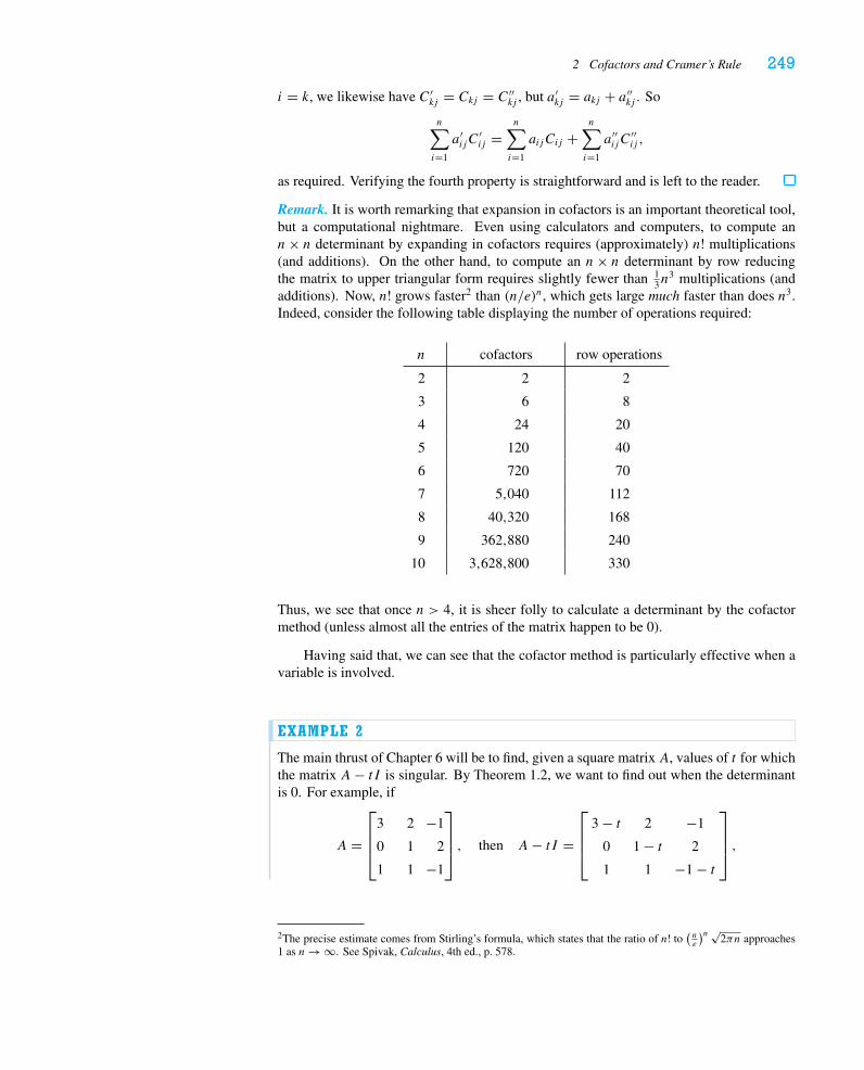
2 Cofactors and Cramer’s Rule 249
i = k, we likewise have C ′kj = Ckj = C ′′
kj , but a′kj = akj + a′′
kj . So
n∑i=1
a′ijC
′ij =
n∑i=1
aijCij +n∑i=1
a′′ijC
′′ij ,
as required. Verifying the fourth property is straightforward and is left to the reader.
Remark. It is worth remarking that expansion in cofactors is an important theoretical tool,but a computational nightmare. Even using calculators and computers, to compute ann× n determinant by expanding in cofactors requires (approximately) n! multiplications(and additions). On the other hand, to compute an n× n determinant by row reducingthe matrix to upper triangular form requires slightly fewer than 1
3n3 multiplications (and
additions). Now, n! grows faster2 than (n/e)n, which gets large much faster than does n3.Indeed, consider the following table displaying the number of operations required:
n cofactors row operations
2 2 2
3 6 8
4 24 20
5 120 40
6 720 70
7 5,040 112
8 40,320 168
9 362,880 240
10 3,628,800 330
Thus, we see that once n > 4, it is sheer folly to calculate a determinant by the cofactormethod (unless almost all the entries of the matrix happen to be 0).
Having said that, we can see that the cofactor method is particularly effective when avariable is involved.
EXAMPLE 2
The main thrust of Chapter 6 will be to find, given a square matrix A, values of t for whichthe matrix A− tI is singular. By Theorem 1.2, we want to find out when the determinantis 0. For example, if
A =
⎡⎢⎢⎣
3 2 −1
0 1 2
1 1 −1
⎤⎥⎥⎦ , then A− tI =
⎡⎢⎢⎣
3 − t 2 −1
0 1 − t 2
1 1 −1 − t
⎤⎥⎥⎦ ,
2The precise estimate comes from Stirling’s formula, which states that the ratio of n! to(ne
)n √2πn approaches
1 as n → ∞. See Spivak, Calculus, 4th ed., p. 578.
250 Chapter 5 Determinants
and we can compute det(A− tI ) by expanding in cofactors along the first column. Notethat this saves us work because one of the terms will drop out.
det(A− tI ) = det
⎡⎢⎢⎣
3 − t 2 −1
0 1 − t 2
1 1 −1 − t
⎤⎥⎥⎦
= (3 − t) det
[1 − t 2
1 −1 − t
]− (0) det
[2 −1
1 −1 − t
]
+ (1) det
[2 −1
1 − t 2
]
= (3 − t)(− (1 − t)(1 + t)− 2)+ (4 + (1 − t))
= (3 − t)(−3 + t2)+ (5 − t)= −t3 + 3t2 + 2t − 4.
In Chapter 6 we will learn some tricks to find the roots of such polynomials.
We conclude this section with a few classic formulas. The first is particularly useful forsolving 2 × 2 systems of equations and may be useful even for larger n if you are interestedonly in a certain component xi of the solution vector.
Proposition 2.3 Cramer’s Rule. Let A be a nonsingular n× n matrix, and let b ∈ Rn.Then the i th coordinate of the vector x solving Ax = b is
xi = detBidetA
,
where Bi is the matrix obtained by replacing the i th column of A by the vector b.
Proof. This is amazingly simple. We calculate the determinant of the matrix obtained byreplacing the i th column of A by b = Ax = x1a1 + · · · + xnan:
detBi = det
⎡⎢⎢⎣
|a1
|
|a2
|· · ·
|x1a1 + · · · + xnan
|· · ·
|an
|
⎤⎥⎥⎦
= det
⎡⎢⎢⎣
|a1
|
|a2
|· · ·
|xiai
|· · ·
|an
|
⎤⎥⎥⎦ = xi detA,
since the multiples of columns other than the i th do not contribute to the determinant.
EXAMPLE 3
We wish to solve [2 3
4 7
][x1
x2
]=[
3
−1
].
2 Cofactors and Cramer’s Rule 251
We have
B1 =[
3 3
−1 7
]and B2 =
[2 3
4 −1
],
so detB1 = 24, detB2 = −14, and detA = 2. Therefore, x1 = 12 and x2 = −7.
We now deduce from Cramer’s Rule an “explicit” formula for the inverse of a non-singular matrix. Students seem always to want an alternative to Gaussian elimination, butwhat follows is practical only for the 2 × 2 case (where it gives us our familiar formulafrom Example 4 on p. 105) and—barely—for the 3 × 3 case. Having an explicit formula,however, can be useful for theoretical purposes.
Proposition 2.4. Let A be a nonsingular matrix, and let C = [Cij]
be the matrix of itscofactors. Then
A−1 = 1
detACT.
Proof. We recall from the discussion on p. 104 that the j th column vector of A−1 is thesolution of Ax = ej , where ej is the j th standard basis vector for Rn. Now, Cramer’s Ruletells us that the i th coordinate of the j th column of A−1 is
(A−1)ij = 1
detAdet Aji ,
where Aji is the matrix obtained by replacing the i th column ofA by ej . Now, we calculatedet Aji by expanding in cofactors along the i th column of the matrix Aji . Since the onlynonzero entry of that column is the j th, and since all its remaining columns are those of theoriginal matrix A, we find that
det Aji = (−1)i+j detAji = Cji,
and this proves the result.
EXAMPLE 4
Let’s apply this result to find the inverse of the matrix
A =
⎡⎢⎢⎣
1 −1 1
2 −1 0
1 −2 2
⎤⎥⎥⎦
without any row operations (compare with the answer obtained by Gaussian elimination onp. 105). First of all,
detA = (1) det
[−1 0
−2 2
]− (−1) det
[2 0
1 2
]+ (1) det
[2 −1
1 −2
]= −1.
Next, we calculate the cofactor matrix. We leave it to the reader to check the details ofthe arithmetic. (Be careful not to forget the checkerboard pattern of +’s and −’s for thecoefficients of the 2 × 2 determinants.)
C =
⎡⎢⎢⎣
−2 −4 −3
0 1 1
1 2 1
⎤⎥⎥⎦ .
252 Chapter 5 Determinants
Thus, applying Proposition 2.4, we have
A−1 = 1
detACT =
⎡⎢⎢⎣
2 0 −1
4 −1 −2
3 −1 −1
⎤⎥⎥⎦ .
In fairness, for 3 × 3 matrices, this formula isn’t bad when detA would cause trouble-some arithmetic doing Gaussian elimination.
EXAMPLE 5
Consider the matrix
A =
⎡⎢⎢⎣
1 2 1
−1 1 2
2 0 3
⎤⎥⎥⎦ ;
then
detA = (1) det
[1 2
0 3
]− (2) det
[−1 2
2 3
]+ (1) det
[−1 1
2 0
]= 15,
and so we suspect the fractions won’t be fun if we do Gaussian elimination. Undaunted,we calculate the cofactor matrix:
C =
⎡⎢⎢⎣
3 7 −2
−6 1 4
3 −3 3
⎤⎥⎥⎦ ,
and so
A−1 = 1
detACT = 1
15
⎡⎢⎢⎣
3 −6 3
7 1 −3
−2 4 3
⎤⎥⎥⎦ .
Exercises 5.2
1. Calculate the following determinants using cofactors.
a. det
⎡⎢⎣
−1 3 5
6 4 2
−2 5 1
⎤⎥⎦
b.∗ det
⎡⎢⎢⎢⎣
1 −1 0 1
0 2 1 1
2 −2 2 3
0 0 6 2
⎤⎥⎥⎥⎦
c. det
⎡⎢⎢⎢⎣
1 4 1 −3
2 10 0 1
0 0 2 2
0 0 −2 1
⎤⎥⎥⎥⎦
d.∗ det
⎡⎢⎢⎢⎢⎢⎢⎣
2 −1 0 0 0
−1 2 −1 0 0
0 −1 2 −1 0
0 0 −1 2 −1
0 0 0 −1 2
⎤⎥⎥⎥⎥⎥⎥⎦
2 Cofactors and Cramer’s Rule 253
2.∗ Let A =⎡⎢⎣
1 2 1
2 3 0
1 4 2
⎤⎥⎦.
a. If Ax =⎡⎢⎣
1
2
−1
⎤⎥⎦, use Cramer’s Rule to find x2.
b. Find A−1 using cofactors.
3.∗ Using cofactors, find the determinant and the inverse of the matrix
A =
⎡⎢⎢⎣
−1 2 3
2 1 0
0 2 3
⎤⎥⎥⎦ .
4. Check that Proposition 2.4 gives the customary answer for the inverse of a nonsingular2 × 2 matrix.
5. For each of the following matrices A, calculate det(A− tI ).
a.∗[
1 5
2 4
]
b.
[0 1
1 0
]
c.
[0 −1
1 0
]
d.
[1 3
3 1
]
e.∗[
1 1
−1 3
]
f.∗
⎡⎢⎣
−1 1 2
1 2 1
2 1 −1
⎤⎥⎦
g.
⎡⎢⎣
1 0 0
−2 1 2
−2 0 3
⎤⎥⎦
h.
⎡⎢⎣
3 2 −2
2 2 −1
2 1 0
⎤⎥⎦
i.
⎡⎢⎣
1 −1 4
3 2 −1
2 1 −1
⎤⎥⎦
j.∗
⎡⎢⎣
1 −6 4
−2 −4 5
−2 −6 7
⎤⎥⎦
6. Show that if the entries of a matrix A are integers, then detA is an integer. (Hint: Useinduction.)
7.� a. Suppose A is an n× n matrix with integer entries and detA = ±1. Show that A−1
has all integer entries.
b. Conversely, suppose A and A−1 are both matrices with integer entries. Prove thatdetA = ±1.
8. We call the vector x ∈ Rn integral if every component xi is an integer. Let A bea nonsingular n× n matrix with integer entries. Prove that the system of equationsAx = b has an integral solution for every integral vector b ∈ Rn if and only if detA =±1. (Note that if A has integer entries, μA maps integral vectors to integral vectors.When does μA map the set of all integral vectors onto the set of all integral vectors?)
9. Prove that the exchange of any pair of rows of a matrix can be accomplished by an oddnumber of exchanges of adjacent pairs.
254 Chapter 5 Determinants
10. Suppose A is an orthogonal n× n matrix. Show that the cofactor matrix C = ±A.
11. Generalizing the result of Proposition 2.4, show thatACT = (detA)I even ifA happensto be singular. In particular, when A is singular, what can you conclude about thecolumns of CT?
12. a. If C is the cofactor matrix of A, give a formula for detC in terms of detA.
b. Let C =⎡⎢⎣
1 −1 2
0 3 1
−1 0 −1
⎤⎥⎦. Can there be a matrix A with cofactor matrix C and
detA = 3? Find a matrix A with positive determinant and cofactor matrix C.
13. a. Show that if (x1, y1) and (x2, y2) are distinct points in R2, then the unique linepassing through them is given by the equation
det
⎡⎢⎢⎣
1 x y
1 x1 y1
1 x2 y2
⎤⎥⎥⎦ = 0.
b. Show that if (x1, y1, z1), (x2, y2, z2), and (x3, y3, z3) are noncollinear points in R3,then the unique plane passing through them is given by the equation
det
⎡⎢⎢⎢⎢⎣
1 x y z
1 x1 y1 z1
1 x2 y2 z2
1 x3 y3 z3
⎤⎥⎥⎥⎥⎦
= 0.
14. As we saw in Exercises 1.6.7 and 1.6.11, through any three noncollinear points in R2
there pass a unique parabola y = ax2 + bx + c and a unique circle x2 + y2 + ax +by + c = 0. (In the case of the parabola, we must also assume that no two of the pointslie on a vertical line.) Given three such points (x1, y1), (x2, y2), and (x3, y3), show thatthe equation of the parabola and circle are, respectively,
det
⎡⎢⎢⎢⎢⎣
1 x x2 y
1 x1 x21 y1
1 x2 x22 y2
1 x3 x23 y3
⎤⎥⎥⎥⎥⎦
= 0 and det
⎡⎢⎢⎢⎢⎣
1 x y x2 + y2
1 x1 y1 x21 + y2
1
1 x2 y2 x22 + y2
2
1 x3 y3 x23 + y2
3
⎤⎥⎥⎥⎥⎦
= 0.
15. (from the 1994 Putnam Exam) Let A and B be 2 × 2 matrices with integer entriessuch that A, A+ B, A+ 2B, A+ 3B, and A+ 4B are all invertible matrices whoseinverses have integer entries. Prove that A+ 5B is invertible and that its inverse hasinteger entries. (Hint: Use Exercise 7.)
16. In this problem, let D(x, y) denote the determinant of the 2 × 2 matrix with rows xand y. Assume the vectors v1, v2, v3 ∈ R2 are pairwise linearly independent.a. Prove that D(v2, v3)v1 +D(v3, v1)v2 +D(v1, v2)v3 = 0. (Hint: Write v1 as a
linear combination of v2 and v3 and use Cramer’s Rule to solve for the coefficients.)
b. Now suppose a1, a2, a3 ∈ R2 and for i = 1, 2, 3, let �i be the line in the planepassing through ai with direction vector vi . Prove that the three lines have a pointin common if and only if
D(a1, v1)D(v2, v3)+D(a2, v2)D(v3, v1)+D(a3, v3)D(v1, v2) = 0.

3 Signed Area in R2 and Signed Volume in R3 255
(Hint: Use Cramer’s Rule to get an equation that says that the point of intersectionof �1 and �2 lies on �3.)
17. Using Exercise 16, prove that the perpendicular bisectors of the sides of a triangle havea common point. (Hint: If ρ : R2 → R2 is rotation through an angle π/2 counterclock-wise, show that D(x, ρ(y)) = x · y.)
3 Signed Area in R2 and SignedVolume in R3
We now turn to the geometric interpretation of the determinant. We start with x, y ∈ R2
and consider the parallelogram P they span. The area of P is nonzero so long as x and yare not collinear, i.e., so long as {x, y} is linearly independent. We want to express the areaof P in terms of the coordinates of x and y. First notice that the area of the parallelogrampictured in Figure 3.1 is the same as the area of the rectangle obtained by moving the shadedtriangle from the right side to the left. This rectangle has area A = bh, where b = ‖x‖ isthe base and h = ‖y‖ sin θ is the height. Remembering that sin θ = cos(π2 − θ) and usingthe fundamental formula for dot product on p. 24, we have (see Figure 3.2)
‖x‖‖y‖ sin θ = ‖x‖‖y‖ cos(π
2− θ)
= ρ(x) · y,
where ρ(x) is the vector obtained by rotating x an angle π/2 counterclockwise. If x =(x1, x2) and y = (y1, y2), then we have
area(P) = ρ(x) · y = (−x2, x1) · (y1, y2) = x1y2 − x2y1,
which we notice is the determinant of the 2 × 2 matrix with row vectors x and y.
x
y
θ
FIGURE 3.1
x
y
θ
ρ(x)
πθ2
−
FIGURE 3.2
EXAMPLE 1
If x = (3, 1) and y = (4, 3), then the area of the parallelogram spanned by x and y isx1y2 − x2y1 = 3 · 3 − 1 · 4 = 5. On the other hand, if we interchange the two, lettingx = (4, 3) and y = (3, 1), then we get x1y2 − x2y1 = 4 · 1 − 3 · 3 = −5. Certainly theparallelogram hasn’t changed, nor does it make sense to have negative area. What is theexplanation? In deriving our formula for the area above, we assumed 0 < θ < π ; but ifwe must turn clockwise to get from x to y, this means that θ is negative, resulting in a signdiscrepancy in the area calculation.
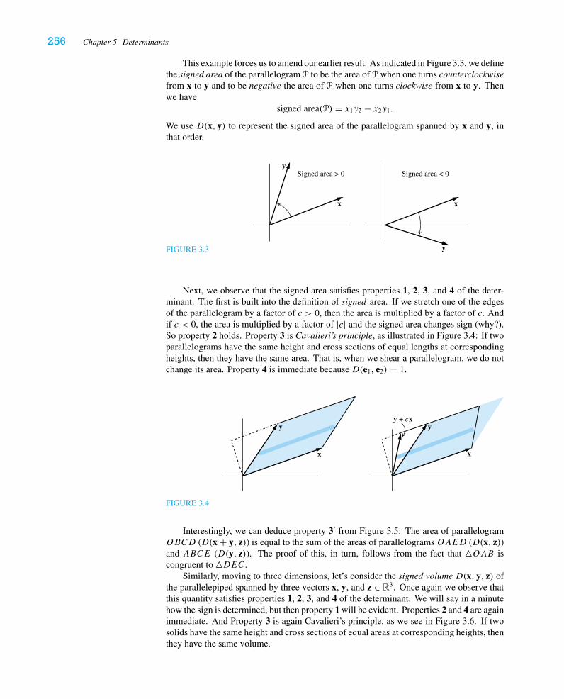
256 Chapter 5 Determinants
This example forces us to amend our earlier result. As indicated in Figure 3.3, we definethe signed area of the parallelogram P to be the area of P when one turns counterclockwisefrom x to y and to be negative the area of P when one turns clockwise from x to y. Thenwe have
signed area(P) = x1y2 − x2y1.
We use D(x, y) to represent the signed area of the parallelogram spanned by x and y, inthat order.
FIGURE 3.3
x
y
x
y
Signed area > 0 Signed area < 0
Next, we observe that the signed area satisfies properties 1, 2, 3, and 4 of the deter-minant. The first is built into the definition of signed area. If we stretch one of the edgesof the parallelogram by a factor of c > 0, then the area is multiplied by a factor of c. Andif c < 0, the area is multiplied by a factor of |c| and the signed area changes sign (why?).So property 2 holds. Property 3 is Cavalieri’s principle, as illustrated in Figure 3.4: If twoparallelograms have the same height and cross sections of equal lengths at correspondingheights, then they have the same area. That is, when we shear a parallelogram, we do notchange its area. Property 4 is immediate because D(e1, e2) = 1.
x x
y yy + cx
FIGURE 3.4
Interestingly, we can deduce property 3′ from Figure 3.5: The area of parallelogramOBCD (D(x + y, z)) is equal to the sum of the areas of parallelogramsOAED (D(x, z))and ABCE (D(y, z)). The proof of this, in turn, follows from the fact that �OAB iscongruent to �DEC.
Similarly, moving to three dimensions, let’s consider the signed volume D(x, y, z) ofthe parallelepiped spanned by three vectors x, y, and z ∈ R3. Once again we observe thatthis quantity satisfies properties 1, 2, 3, and 4 of the determinant. We will say in a minutehow the sign is determined, but then property 1 will be evident. Properties 2 and 4 are againimmediate. And Property 3 is again Cavalieri’s principle, as we see in Figure 3.6. If twosolids have the same height and cross sections of equal areas at corresponding heights, thenthey have the same volume.
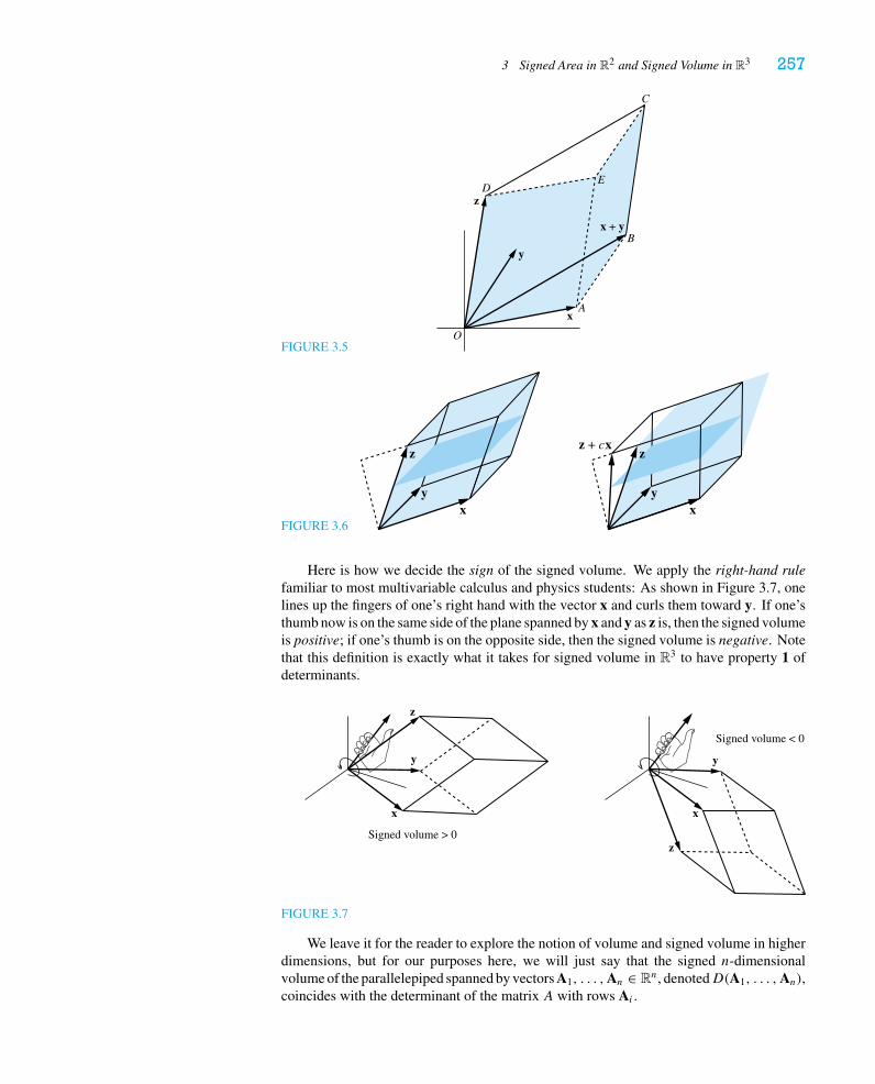
3 Signed Area in R2 and Signed Volume in R3 257
FIGURE 3.5
x
z
y
x + y
O
A
B
C
DE
FIGURE 3.6x
y
z
x
z + cx
y
z
Here is how we decide the sign of the signed volume. We apply the right-hand rulefamiliar to most multivariable calculus and physics students: As shown in Figure 3.7, onelines up the fingers of one’s right hand with the vector x and curls them toward y. If one’sthumb now is on the same side of the plane spanned by x and y as z is, then the signed volumeis positive; if one’s thumb is on the opposite side, then the signed volume is negative. Notethat this definition is exactly what it takes for signed volume in R3 to have property 1 ofdeterminants.
x
y
z
z
x
y
Signed volume > 0
Signed volume < 0
FIGURE 3.7
We leave it for the reader to explore the notion of volume and signed volume in higherdimensions, but for our purposes here, we will just say that the signed n-dimensionalvolume of the parallelepiped spanned by vectors A1, . . . ,An ∈ Rn, denotedD(A1, . . . ,An),coincides with the determinant of the matrix A with rows Ai .
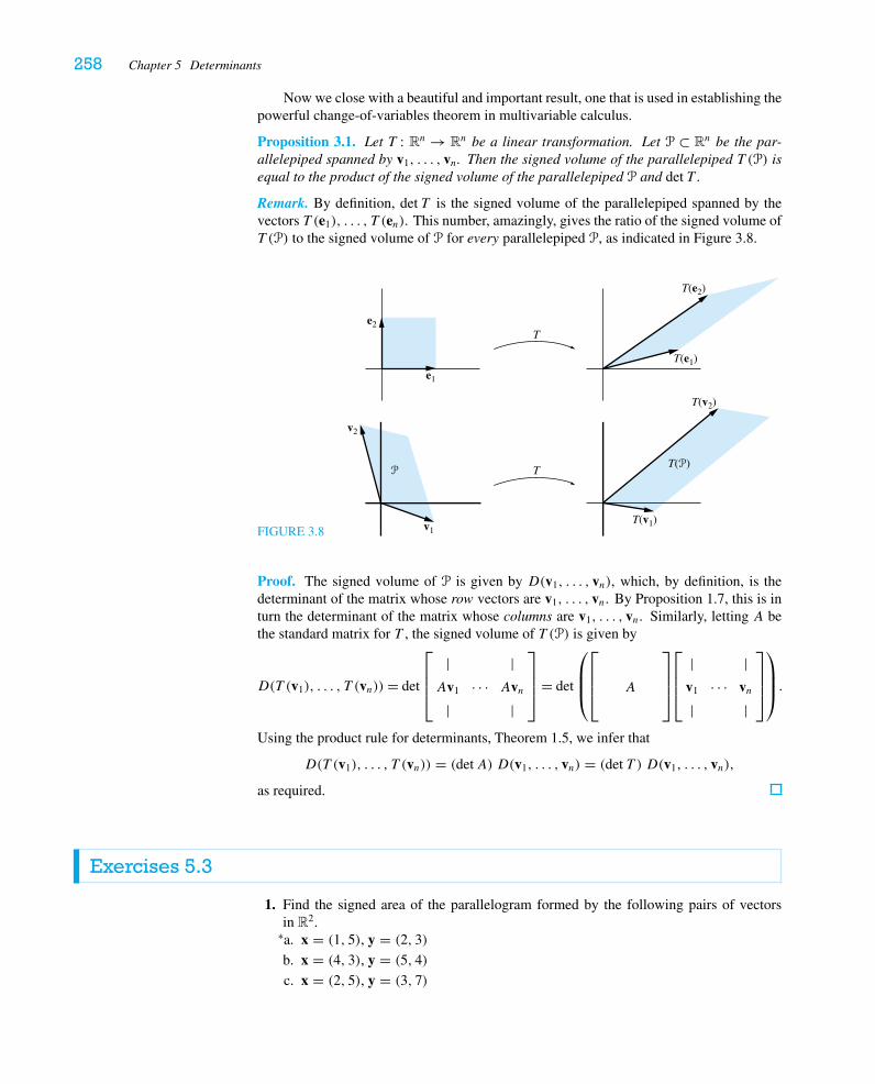
258 Chapter 5 Determinants
Now we close with a beautiful and important result, one that is used in establishing thepowerful change-of-variables theorem in multivariable calculus.
Proposition 3.1. Let T : Rn → Rn be a linear transformation. Let P ⊂ Rn be the par-allelepiped spanned by v1, . . . , vn. Then the signed volume of the parallelepiped T (P) isequal to the product of the signed volume of the parallelepiped P and det T .
Remark. By definition, det T is the signed volume of the parallelepiped spanned by thevectors T (e1), . . . , T (en). This number, amazingly, gives the ratio of the signed volume ofT (P) to the signed volume of P for every parallelepiped P, as indicated in Figure 3.8.
FIGURE 3.8
e2
e1
v2
v1
T(e2)
T(e1)
T(v2)
T(v1)
T(P)
T
TP
Proof. The signed volume of P is given by D(v1, . . . , vn), which, by definition, is thedeterminant of the matrix whose row vectors are v1, . . . , vn. By Proposition 1.7, this is inturn the determinant of the matrix whose columns are v1, . . . , vn. Similarly, letting A bethe standard matrix for T , the signed volume of T (P) is given by
D(T (v1), . . . , T (vn))= det
⎡⎢⎢⎣
| |Av1 · · · Avn
| |
⎤⎥⎥⎦= det
⎛⎜⎜⎝
⎡⎢⎢⎣ A
⎤⎥⎥⎦
⎡⎢⎢⎣
| |v1 · · · vn
| |
⎤⎥⎥⎦
⎞⎟⎟⎠.
Using the product rule for determinants, Theorem 1.5, we infer that
D(T (v1), . . . , T (vn)) = (detA) D(v1, . . . , vn) = (det T ) D(v1, . . . , vn),
as required.
Exercises 5.3
1. Find the signed area of the parallelogram formed by the following pairs of vectorsin R2.a.∗ x = (1, 5), y = (2, 3)
b. x = (4, 3), y = (5, 4)
c. x = (2, 5), y = (3, 7)
3 Signed Area in R2 and Signed Volume in R3 259
2. Find the signed volume of the parallelepiped formed by the following triples of vectorsin R3.a.∗ x = (1, 2, 1), y = (2, 3, 1), z = (−1, 0, 3)
b. x = (1, 1, 1), y = (2, 3, 4), z = (1, 1, 5)
c. x = (3,−1, 2), y = (1, 0,−3), z = (−2, 1,−1)
3. LetA = (a1, a2), B = (b1, b2), andC = (c1, c2) be points in R2. Show that the signedarea of �ABC is given by
1
2det
⎡⎢⎢⎣
1 a1 a2
1 b1 b2
1 c1 c2
⎤⎥⎥⎦ .
4. Suppose A, B, and C are vertices of a triangle in R2, and D is a point in R2.a. Use the fact that the vectors
−→AB and
−→AC are linearly independent to prove that
we can write D = rA+ sB + tC for some scalars r , s, and t with r + s + t = 1.(Here, we are treating A, B, C, and D as vectors in R2.)
b. Use Exercise 3 to show that t is the ratio of the signed area of �ABD to the signedarea of �ABC (and similar results hold for r and s).
5. Let u, v ∈ R3. Define the cross product of u and v to be the vector
u × v =(
det
[u2 u3
v2 v3
], det
[u3 u1
v3 v1
], det
[u1 u2
v1 v2
]).
a. Prove that for any vectors u, v, and w ∈ R3, w · (u × v) = D(w, u, v).b. Show that u × v is orthogonal to u and v.
6. Let P be the parallelogram spanned by two vectors u, v ∈ R3.a. By interpreting D(u × v, u, v) as both a signed volume and a determinant, show
that area(P) = ‖u × v‖. (Hint: For the latter, expand in cofactors.)
b. Let P1 be the projection of P onto the x2x3-plane; P2, its projection onto the x1x3-plane; and P3, its projection onto the x1x2-plane. Show that
(area(P)
)2 = (area(P1)
)2 + (area(P2)
)2 + (area(P3)
)2 .
How’s that for a generalization of the Pythagorean Theorem?!
7. Let a ∈ R3 be fixed. Define T : R3 → R3 by T (x) = a × x (see Exercise 5).a. Prove that T is a linear transformation.
b. Give the standard matrix A of T .
c. Explain, using part a of Exercise 5 and Proposition 5.2 of Chapter 2, why A isskew-symmetric.
8. Suppose a polygon in the plane has vertices (x1, y1), (x2, y2), . . . , (xn, yn). Give aformula for its area. (Hint: To start, assume that the origin is inside the polygon; drawa picture.)
9. (from the 1994 Putnam Exam) Find the value of m so that the line y = mx bisects theregion {
(x, y) ∈ R2 : x2
4+ y2 ≤ 1, x ≥ 0, y ≥ 0
}.
(Hint: How are ellipses, circles, and linear transformations related?)
10. Given any ellipse, show that there are infinitely many inscribed triangles of maximalarea. (Hint: See the hint for Exercise 9.)
260 Chapter 5 Determinants
11. Let x, y ∈ R3. Show that
det
[x · x x · y
y · x y · y
]
is the square of the area of the parallelogram spanned by x and y.
12. Generalizing the result of Exercise 11, let v1, . . . , vk ∈ Rn. Show that
det
⎡⎢⎢⎢⎢⎢⎣
v1 · v1 v1 · v2 . . . v1 · vk
v2 · v1 v2 · v2 . . . v2 · vk...
.... . .
...
vk · v1 vk · v2 . . . vk · vk
⎤⎥⎥⎥⎥⎥⎦
is the square of the volume of the k-dimensional parallelepiped spanned by v1, . . . , vk .
HISTORICAL NOTESDeterminants first arose as an aid to solving equations. Although 2 × 2 determinants wereimplicit in the solution of a system of two linear equations in two unknowns given by Giro-lamo Cardano (1501–1576) in his work Ars Magna (1545), the Japanese mathematicianTakakazu Seki (1642–1708) is usually credited with a more general study of determinants.Seki, the son of a samurai, was a self-taught mathematical prodigy who developed quite afollowing in seventeenth-century Japan. In 1683 he published Method of Solving Dissim-ulated Problems, in which he studied determinants of matrices at least as large as 5 × 5.In the same year the German mathematician Gottfried Wilhelm von Leibniz (1646–1716)wrote a letter to Guillaume de l’Hôpital (1661–1704), in which he gave the vanishing ofthe determinant of a 3 × 3 system of linear equations as the condition for the homogeneoussystem to have a nontrivial solution. Although Leibniz never published his work on deter-minants, his notes show that he understood many of their properties and uses, as well asmethods for computing them.
After Seki and Leibniz, determinants found their way into the work of many mathemati-cians. In 1750 the Swiss mathematician Gabriel Cramer (1704–1752) published, withoutproof and as an appendix to a book on plane algebraic curves, what is now called Cramer’sRule. Other eighteenth-century mathematicians who studied methods for computing de-terminants and uses for them were Étienne Bézout (1730–1783), Alexandre Vandermonde(1735–1796), and Pierre-Simon Laplace (1749–1847), who developed the method of ex-pansion by cofactors for computing determinants.
The French mathematician Joseph-Louis Lagrange (1736–1813) seems to have beenthe first to notice the relationship between determinants and volume. In 1773 he used a3 × 3 determinant to compute the volume of a tetrahedron. Carl Friedrich Gauss (1777–1855) used matrices to study the properties of quadratic forms (see Section 4 of Chapter 6).Augustin Louis Cauchy (1789–1857) also studied determinants in the context of quadraticforms and is given credit for the first proof of the multiplicative properties of the determinant.Finally, three papers that Carl Gustav Jacob Jacobi (1804–1851) wrote in 1841 broughtgeneral attention to the theory of determinants. Jacobi, a brilliant German mathematicianwhose life was cut short by smallpox, focused his attention on determinants of matriceswith functions as entries. He proved key results regarding the independence of sets offunctions, inventing a particular determinant that is now called the Jacobian determinant. Itplays a major role in the change-of-variables formula in multivariable calculus, generalizingProposition 3.1.
261
C H A P T E R 6EIGENVALUES AND EIGENVECTORS
W e suggested in Chapter 4 that a linear transformation T : V → V is best understoodwhen there is a basis for V with respect to which the matrix of T becomes diagonal.
In this chapter, we shall develop techniques for determining whether T is diagonalizableand, if so, for finding a diagonalizing basis.
There are important reasons to diagonalize a matrix. For instance, we saw a longwhile ago (for example, in Examples 6 through 9 in Section 6 of Chapter 1) that it is oftennecessary to understand and calculate (high) powers of a given square matrix. SupposeA isdiagonalizable, i.e., there is an invertible matrix P so that P−1AP = � is diagonal. Thenwe have
A = P�P−1, and so
Ak = (P�P−1)(P�P−1) · · · (P�P−1)︸ ︷︷ ︸k times
= P�kP−1,
using associativity to regroup and cancel the P−1P pairs. Since �k is easy to calculate,we are left with a formula for Ak that helps us understand the corresponding linear trans-formation and is easy to compute. We will see a number of applications of this principlein Section 3. Indeed, we will see that the entries of � tell us a lot about growth in discretedynamical systems and whether systems approach a “steady state” in time. Further appli-cations, to understanding conic sections and quadric surfaces and to systems of differentialequations, are given in Section 4 and in Section 3 of Chapter 7, respectively.
We turn first to the matter of finding the diagonal matrix� if, in fact,A is diagonalizable.Then we will develop some criteria that guarantee diagonalizability.
1 The Characteristic Polynomial
Recall that a linear transformation T : V → V is diagonalizable if there is an (ordered)basis B = {v1, . . . , vn} for V so that the matrix for T with respect to that basis is diagonal.This means precisely that, for some scalars λ1, . . . , λn, we have
T (v1) = λ1v1,
T (v2) = λ2v2,
...
T (vn) = λnvn.
262 Chapter 6 Eigenvalues and Eigenvectors
Likewise, an n× n matrix A is diagonalizable if the associated linear transformationμA : Rn → Rn is diagonalizable; so A is diagonalizable precisely when there is a basis{v1, . . . , vn} for Rn with the property that Avi = λivi for all i = 1, . . . , n. We can writethese equations in matrix form:
A
⎡⎢⎢⎣
|v1
|
|v2
|· · ·
|vn
|
⎤⎥⎥⎦ =
⎡⎢⎢⎣
|v1
|
|v2
|· · ·
|vn
|
⎤⎥⎥⎦
⎡⎢⎢⎢⎢⎣
λ1
λ2. . .
λn
⎤⎥⎥⎥⎥⎦.
Thus, if we let P be the n× n matrix whose columns are the vectors v1, . . . , vn and � bethe n× n diagonal matrix with diagonal entries λ1, . . . , λn, then we have
AP = P�, and so P−1AP = �.
(Of course, this all follows immediately from the change-of-basis formula, Proposition 3.2of Chapter 4. In that context, we called P the change-of-basis matrix.)
This observation leads us to the following definition.
Definition. Let T : V → V be a linear transformation. A nonzero vector v ∈ V is calledan eigenvector1 of T if there is a scalar λ so that T (v) = λv. The scalar λ is called theassociated eigenvalue of T .
In other words, an eigenvector of a linear transformation T is a nonzero vector that isrescaled (perhaps in the negative direction) by T . The line spanned by the vector is identicalto the line spanned by its image under T .
EXAMPLE 1
Revisiting Example 8 in Section 3 of Chapter 4, we see that the vectors v1 and v2 areeigenvectors of T , with associated eigenvalues 4 and 1.
This definition, in turn, leads to a convenient reformulation of diagonalizability:
Proposition 1.1. The linear transformation T : V → V is diagonalizable if and only ifthere is a basis for V consisting of eigenvectors of T .
At this juncture, the obvious question to ask is how we should find eigenvectors. As amatter of convenience, we’re now going to stick mostly to the more familiar matrix notationsince we’ll be starting with an n× n matrix most of the time anyhow. For general lineartransformations, let A denote the matrix for T with respect to some basis. Let’s start byobserving that the set of eigenvectors with eigenvalue λ, together with the zero vector,forms a subspace.
1In the old days, it was called a characteristic vector, more or less a literal translation of the German eigen, whichmeans “characteristic,” “proper,” or “particular.”
1 The Characteristic Polynomial 263
Lemma 1.2. Let A be an n× n matrix, and let λ be any scalar. Then
E(λ) = {x ∈ Rn : Ax = λx} = N(A− λI)is a subspace of Rn. Moreover, E(λ) �= {0} if and only if λ is an eigenvalue, in which casewe call E(λ) the λ-eigenspace of the matrix A.
Proof. We know that N(A− λI) is always a subspace of Rn. By definition, λ is aneigenvalue precisely when there is a nonzero vector in E(λ).
We now come to what will be for us the main computational tool for finding eigenvalues.
Proposition 1.3. Let A be an n× n matrix. Then λ is an eigenvalue of A if and only ifdet(A− λI) = 0.
Proof. From Lemma 1.2 we infer that λ is an eigenvalue if and only if the matrixA− λI issingular. Next we conclude from Theorem 1.2 of Chapter 5 thatA− λI is singular preciselywhen det(A− λI) = 0. Putting the two statements together, we obtain the result.
Once we use this criterion to find the eigenvalues λ, it is an easy matter to find thecorresponding eigenvectors merely by finding N(A− λI).
EXAMPLE 2
Let’s find the eigenvalues and eigenvectors of the matrix
A =[
3 1
−3 7
].
We start by calculating
det(A− tI ) = det
[3 − t 1
−3 7 − t
]= (3 − t)(7 − t)− (1)(−3) = t2 − 10t + 24.
Since t2 − 10t + 24 = (t − 4)(t − 6) = 0 when t = 4 or t = 6, these are our two eigen-values. We now proceed to find the corresponding eigenspaces.
E(4): We see that
v1 =[
1
1
]gives a basis for N(A− 4I ) = N
([−1 1
−3 3
]).
E(6): We see that
v2 =[
1
3
]gives a basis for N(A− 6I ) = N
([−3 1
−3 1
]).
Since we observe that the set {v1, v2} is linearly independent, the matrixA is diagonalizable.
Indeed, as the reader can check, if we take P =[
1 1
1 3
], then
P−1AP =[
32 − 1
2
− 12
12
][3 1
−3 7
][1 1
1 3
]=[
4 0
0 6
],
as should be the case.
264 Chapter 6 Eigenvalues and Eigenvectors
EXAMPLE 3
Let’s find the eigenvalues and eigenvectors of the matrix
A =
⎡⎢⎢⎣
1 2 1
0 1 0
1 3 1
⎤⎥⎥⎦ .
We begin by computing
det(A− tI ) = det
⎡⎢⎢⎣
1 − t 2 1
0 1 − t 0
1 3 1 − t
⎤⎥⎥⎦
(expanding in cofactors along the second row)
= (1 − t)((1 − t)(1 − t)− 1) = (1 − t)(t2 − 2t) = −t (t − 1)(t − 2).
Thus, the eigenvalues of A are λ = 0, 1, and 2. We next find the respective eigenspaces.
E(0): We see that
v1 =
⎡⎢⎢⎣
−1
0
1
⎤⎥⎥⎦ gives a basis for N(A− 0I ) = N
⎛⎜⎜⎝
⎡⎢⎢⎣
1 2 1
0 1 0
1 3 1
⎤⎥⎥⎦
⎞⎟⎟⎠
= N
⎛⎜⎜⎝
⎡⎢⎢⎣
1 0 1
0 1 0
0 0 0
⎤⎥⎥⎦
⎞⎟⎟⎠ .
E(1): We see that
v2 =
⎡⎢⎢⎣
3
−1
2
⎤⎥⎥⎦ gives a basis for N(A− 1I ) = N
⎛⎜⎜⎝
⎡⎢⎢⎣
0 2 1
0 0 0
1 3 0
⎤⎥⎥⎦
⎞⎟⎟⎠
= N
⎛⎜⎜⎝
⎡⎢⎢⎣
1 0 − 32
0 1 12
0 0 0
⎤⎥⎥⎦
⎞⎟⎟⎠ .
E(2): We see that
v3 =
⎡⎢⎢⎣
1
0
1
⎤⎥⎥⎦ gives a basis for N(A− 2I ) = N
⎛⎜⎜⎝
⎡⎢⎢⎣
−1 2 1
0 −1 0
1 3 −1
⎤⎥⎥⎦
⎞⎟⎟⎠
= N
⎛⎜⎜⎝
⎡⎢⎢⎣
1 0 −1
0 1 0
0 0 0
⎤⎥⎥⎦
⎞⎟⎟⎠ .
Once again,A is diagonalizable. As the reader can check, {v1, v2, v3} is linearly independent
1 The Characteristic Polynomial 265
and therefore gives a basis for R3. Just to be sure, we let
P =
⎡⎢⎢⎣
−1 3 1
0 −1 0
1 2 1
⎤⎥⎥⎦ ;
then
P−1AP =
⎡⎢⎢⎣
− 12 − 1
212
0 −1 012
52
12
⎤⎥⎥⎦
⎡⎢⎢⎣
1 2 1
0 1 0
1 3 1
⎤⎥⎥⎦
⎡⎢⎢⎣
−1 3 1
0 −1 0
1 2 1
⎤⎥⎥⎦ =
⎡⎢⎢⎣
0 0 0
0 1 0
0 0 2
⎤⎥⎥⎦ ,
as we expected.
There is a built-in check here for the eigenvalues. If λ is truly to be an eigenvalue ofA, we must find a nonzero vector in N(A− λI). If we do not, then λ cannot be aneigenvalue.
EXAMPLE 4
Let’s find the eigenvalues and eigenvectors of the matrix
A =[
0 −1
1 0
].
As usual, we calculate
det(A− tI ) = det
[−t −1
1 −t
]= t2 + 1.
Since t2 + 1 ≥ 1 for all real numbers t , there is no real number λ so that det(A− λI) = 0.Thus, the matrix A has no real eigenvalue. Nevertheless, it is still interesting to alloweigenvalues to be complex numbers (and, then, eigenvectors to be vectors with complexentries). We will study this in greater detail in Section 1 of Chapter 7.
We recognize A as the matrix giving rotation of R2 through an angle of π/2. Thus, itis clear on geometric grounds that this matrix has no (real) eigenvector: For any nonzerovector x, the vector Ax makes a right angle with x and is therefore not a scalar multipleof x.2
It is evident that we are going to find the eigenvalues of a matrixA by finding the (real)roots of the polynomial det(A− tI ). This leads us to make our next definition.
Definition. Let A be a square matrix. Then p(t) = pA(t) = det(A− tI ) is called thecharacteristic polynomial of A.3
2On the other hand, from the complex perspective, we note that ±i are the (complex) eigenvalues of A, andmultiplying a complex number by i has the effect of rotating it an angle of π/2. The reader can check that thecomplex eigenvectors of this matrix are (1,±i).3That the characteristic polynomial of an n× n matrix is in fact a polynomial of degree n seems pretty evidentfrom examples, but the fastidious reader can establish this by expanding in cofactors.
266 Chapter 6 Eigenvalues and Eigenvectors
We can restate Proposition 1.3 by saying that the eigenvalues of A are the real rootsof the characteristic polynomial pA(t). As in Example 4, this polynomial may sometimeshave complex roots; we will abuse language by calling these roots complex eigenvalues.See Section 1 of Chapter 7 for a more detailed discussion of this situation.
Lemma 1.4. If A and B are similar matrices, then pA(t) = pB(t).
Proof. Suppose B = P−1AP . Then
pB(t)= det(B − tI )= det(P−1AP − tI )= det(P−1(A− tI )P )= det(A− tI )=pA(t),
by virtue of the product rule for determinants, Theorem 1.5 of Chapter 5.
As a consequence, if V is a finite-dimensional vector space and T : V → V is a lineartransformation, then we can define the characteristic polynomial of T to be that of the matrixA for T with respect to any basis for V . By the change-of-basis formula, Proposition 3.2of Chapter 4, and Lemma 1.4, we’ll get the same answer no matter what basis we choose.
Remark. In order to determine the eigenvalues of a matrix, we must find the roots ofits characteristic polynomial. In real-world applications (where the matrices tend to getquite large), one might do this numerically (e.g., using Newton’s method). However, thereare more sophisticated methods for finding the eigenvalues without even calculating thecharacteristic polynomial; a powerful such method is based on theQR decomposition of amatrix. The interested reader should consult Strang’s books or Wilkinson for more details.
For the lion’s share of the matrices that we shall encounter here, the eigenvalues willbe integers, and so we take this opportunity to remind you of a shortcut from high schoolalgebra.
Proposition 1.5 (Rational Roots Test). Let p(t) = antn + an−1t
n−1 + · · · + a1t + a0 bea polynomial with integer coefficients. If t = r/s is a rational root (in lowest terms) of p(t),then r must be a factor of a0 and s must be a factor of an.4
In particular, when the leading coefficient an is ±1, as is always the case with thecharacteristic polynomial, any rational root must in fact be an integer that divides a0. So,in practice, we test the various factors of a0 (being careful to try both positive and negativefactors). In our case, a0 = p(0) = detA, so, starting with a matrixAwith all integer entries,only the factors of the integer detA can be integer eigenvalues. Once we find one root λ,we can divide p(t) by t − λ to obtain a polynomial of smaller degree.
EXAMPLE 5
The characteristic polynomial of the matrix
A =
⎡⎢⎢⎣
4 −3 3
0 1 4
2 −2 1
⎤⎥⎥⎦
is p(t) = −t3 + 6t2 − 11t + 6. The factors of 6 are ±1, ±2, ±3, and ±6. Since p(1) = 0,we know that 1 is a root (so we were lucky!). Now,
−p(t)t − 1
= t2 − 5t + 6 = (t − 2)(t − 3),
and we have succeeded in finding all three eigenvalues of A, namely, λ = 1, 2, and 3.
4We do not include a proof here, but you can find one in most abstract algebra texts. For obvious reasons, werecommend Shifrin’s Abstract Algebra: A Geometric Approach, p. 105.
1 The Characteristic Polynomial 267
Remark. It might be nice to have a few shortcuts for calculating the characteristic polynomialof small matrices. For 2 × 2 matrices, it’s quite easy:
det
[a − t b
c d − t
]= (a − t)(d − t)− bc = t2 − (a + d) t + (ad − bc)
= t2 − trA t + detA .
(Recall that the trace of a matrix A, denoted trA, is the sum of its diagonal entries.) For3 × 3 matrices, it’s a bit more involved:
det
⎡⎢⎢⎣a11 − t a12 a13
a21 a22 − t a23
a31 a32 a33 − t
⎤⎥⎥⎦ = −t3 + (a11 + a22 + a33) t
2
− ((a11a22 − a12a21)+ (a11a33 − a13a31)+ (a22a33 − a23a32)
)t
+ (a11a22a33 + a12a23a31 + a13a21a32 − a13a22a31 − a11a23a32 − a12a21a33)
= −t3 + trA t2 − Fred t + detA .
The coefficient of t in the characteristic polynomial has no standard name, and so it was thatone of the authors’ students christened the expression Fred years ago. Nevertheless, we seethat Fred is the sum of the cofactors C11, C22, and C33, i.e., the sum of the determinants ofthe (three) 2 × 2 submatrices formed by deleting identical rows and columns from A.
In general, the characteristic polynomial p(t) of an n× n matrix A is always of theform
p(t) = (−1)ntn + (−1)n−1 trA tn−1 + (−1)n−2 Fred tn−2 + · · · + detA .
Note that the constant coefficient is always detA (with no minus signs) because p(0) =det(A− 0I ) = detA.
In the long run, these formulas notwithstanding, it’s sometimes best to calculate thecharacteristic polynomial of 3 × 3 matrices by expansion in cofactors. If one is both atten-tive and fortunate, this may save the trouble of factoring the polynomial.
EXAMPLE 6
Let’s find the characteristic polynomial of
A =
⎡⎢⎢⎣
2 0 0
1 2 1
0 1 2
⎤⎥⎥⎦ .
We calculate the determinant by expanding in cofactors along the first row:
det
⎡⎢⎢⎣
2 − t 0 0
1 2 − t 1
0 1 2 − t
⎤⎥⎥⎦ = (2 − t) det
[2 − t 1
1 2 − t
]
= (2 − t)((2 − t)2 − 1) = (2 − t)(t2 − 4t + 3)
= (2 − t)(t − 3)(t − 1).
268 Chapter 6 Eigenvalues and Eigenvectors
But that was too easy. Let’s try the characteristic polynomial of
B =
⎡⎢⎢⎣
2 0 1
1 3 1
1 1 2
⎤⎥⎥⎦ .
Again, we expand in cofactors along the first row:
det
⎡⎢⎢⎣
2 − t 0 1
1 3 − t 1
1 1 2 − t
⎤⎥⎥⎦ = (2 − t) det
[3 − t 1
1 2 − t
]+ 1 det
[1 3 − t1 1
]
= (2 − t)((3 − t)(2 − t)− 1)+ (1 − (3 − t))
= (2 − t)(t2 − 5t + 5)− (2 − t) = (2 − t)(t2 − 5t + 4)
= (2 − t)(t − 1)(t − 4).
OK, perhaps we were a bit lucky there, too.
Exercises 6.1
1. Find the eigenvalues and eigenvectors of the following matrices.
a.∗[
1 5
2 4
]
b.
[0 1
1 0
]
c.
[10 −6
18 −11
]
d.
[0 1
−1 0
]
e.
[1 3
3 1
]
f.∗[
1 1
−1 3
]
g.∗
⎡⎢⎣
−1 1 2
1 2 1
2 1 −1
⎤⎥⎦
h.
⎡⎢⎣
1 0 0
−2 1 2
−2 0 3
⎤⎥⎦
i.
⎡⎢⎣
1 −1 2
0 1 0
0 −2 3
⎤⎥⎦
j.∗
⎡⎢⎣
2 0 1
0 1 2
0 0 1
⎤⎥⎦
k.
⎡⎢⎣
1 −2 2
−1 0 −1
0 2 −1
⎤⎥⎦
l.
⎡⎢⎣
3 1 0
0 1 2
0 1 2
⎤⎥⎦
m.
⎡⎢⎣
1 −1 4
3 2 −1
2 1 −1
⎤⎥⎦
n.∗
⎡⎢⎣
1 −6 4
−2 −4 5
−2 −6 7
⎤⎥⎦
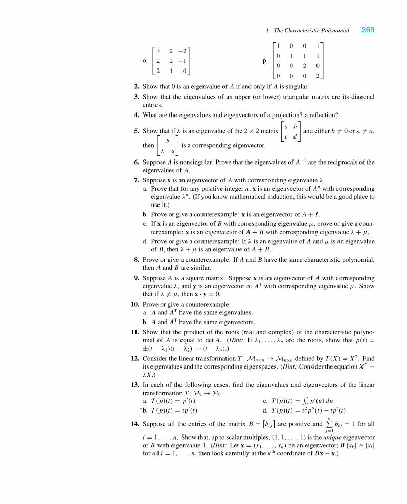
1 The Characteristic Polynomial 269
o.
⎡⎢⎣
3 2 −2
2 2 −1
2 1 0
⎤⎥⎦ p.
⎡⎢⎢⎢⎣
1 0 0 1
0 1 1 1
0 0 2 0
0 0 0 2
⎤⎥⎥⎥⎦
2. Show that 0 is an eigenvalue of A if and only if A is singular.
3. Show that the eigenvalues of an upper (or lower) triangular matrix are its diagonalentries.
4. What are the eigenvalues and eigenvectors of a projection? a reflection?
5. Show that if λ is an eigenvalue of the 2 × 2 matrix
[a b
c d
]and either b �= 0 or λ �= a,
then
[b
λ− a
]is a corresponding eigenvector.
6. Suppose A is nonsingular. Prove that the eigenvalues of A−1 are the reciprocals of theeigenvalues of A.
7. Suppose x is an eigenvector of A with corresponding eigenvalue λ.a. Prove that for any positive integer n, x is an eigenvector of An with corresponding
eigenvalue λn. (If you know mathematical induction, this would be a good place touse it.)
b. Prove or give a counterexample: x is an eigenvector of A+ I .
c. If x is an eigenvector of B with corresponding eigenvalue μ, prove or give a coun-terexample: x is an eigenvector of A+ B with corresponding eigenvalue λ+ μ.
d. Prove or give a counterexample: If λ is an eigenvalue of A and μ is an eigenvalueof B, then λ+ μ is an eigenvalue of A+ B.
8. Prove or give a counterexample: If A and B have the same characteristic polynomial,then A and B are similar.
9. Suppose A is a square matrix. Suppose x is an eigenvector of A with correspondingeigenvalue λ, and y is an eigenvector of AT with corresponding eigenvalue μ. Showthat if λ �= μ, then x · y = 0.
10. Prove or give a counterexample:a. A and AT have the same eigenvalues.
b. A and AT have the same eigenvectors.
11. Show that the product of the roots (real and complex) of the characteristic polyno-mial of A is equal to detA. (Hint: If λ1, . . . , λn are the roots, show that p(t) =±(t − λ1)(t − λ2) · · · (t − λn).)
12. Consider the linear transformation T : Mn×n → Mn×n defined by T (X) = XT. Findits eigenvalues and the corresponding eigenspaces. (Hint: Consider the equationXT =λX.)
13. In each of the following cases, find the eigenvalues and eigenvectors of the lineartransformation T : P3 → P3.a. T (p)(t) = p′(t)b.∗ T (p)(t) = tp′(t)
c. T (p)(t) = ∫ t0 p′(u) dud. T (p)(t) = t2p′′(t)− tp′(t)
14. Suppose all the entries of the matrix B = [bij]
are positive andn∑j=1bij = 1 for all
i = 1, . . . , n. Show that, up to scalar multiples, (1, 1, . . . , 1) is the unique eigenvectorof B with eigenvalue 1. (Hint: Let x = (x1, . . . , xn) be an eigenvector; if |xk| ≥ |xi |for all i = 1, . . . , n, then look carefully at the kth coordinate of Bx − x.)
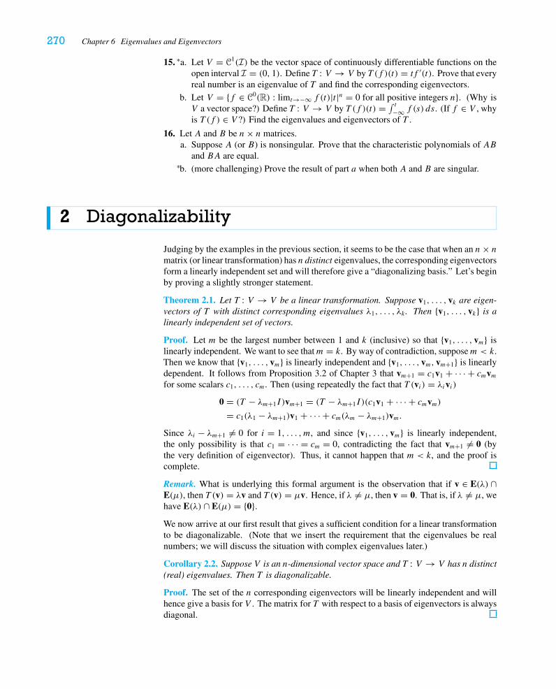
270 Chapter 6 Eigenvalues and Eigenvectors
15. a.∗ Let V = C1(I) be the vector space of continuously differentiable functions on theopen interval I = (0, 1). Define T : V → V by T (f )(t) = tf ′(t). Prove that everyreal number is an eigenvalue of T and find the corresponding eigenvectors.
b. Let V = {f ∈ C0(R) : limt→−∞ f (t)|t |n = 0 for all positive integers n}. (Why isV a vector space?) Define T : V → V by T (f )(t) = ∫ t−∞ f (s) ds. (If f ∈ V , whyis T (f ) ∈ V ?) Find the eigenvalues and eigenvectors of T .
16. Let A and B be n× n matrices.a. Suppose A (or B) is nonsingular. Prove that the characteristic polynomials of AB
and BA are equal.
b.∗ (more challenging) Prove the result of part a when both A and B are singular.
2 Diagonalizability
Judging by the examples in the previous section, it seems to be the case that when an n× nmatrix (or linear transformation) has n distinct eigenvalues, the corresponding eigenvectorsform a linearly independent set and will therefore give a “diagonalizing basis.” Let’s beginby proving a slightly stronger statement.
Theorem 2.1. Let T : V → V be a linear transformation. Suppose v1, . . . , vk are eigen-vectors of T with distinct corresponding eigenvalues λ1, . . . , λk . Then {v1, . . . , vk} is alinearly independent set of vectors.
Proof. Let m be the largest number between 1 and k (inclusive) so that {v1, . . . , vm} islinearly independent. We want to see thatm = k. By way of contradiction, supposem < k.Then we know that {v1, . . . , vm} is linearly independent and {v1, . . . , vm, vm+1} is linearlydependent. It follows from Proposition 3.2 of Chapter 3 that vm+1 = c1v1 + · · · + cmvmfor some scalars c1, . . . , cm. Then (using repeatedly the fact that T (vi ) = λivi)
0 = (T − λm+1I )vm+1 = (T − λm+1I )(c1v1 + · · · + cmvm)
= c1(λ1 − λm+1)v1 + · · · + cm(λm − λm+1)vm.
Since λi − λm+1 �= 0 for i = 1, . . . , m, and since {v1, . . . , vm} is linearly independent,the only possibility is that c1 = · · · = cm = 0, contradicting the fact that vm+1 �= 0 (bythe very definition of eigenvector). Thus, it cannot happen that m < k, and the proof iscomplete.
Remark. What is underlying this formal argument is the observation that if v ∈ E(λ) ∩E(μ), then T (v) = λv and T (v) = μv. Hence, if λ �= μ, then v = 0. That is, if λ �= μ, wehave E(λ) ∩ E(μ) = {0}.We now arrive at our first result that gives a sufficient condition for a linear transformationto be diagonalizable. (Note that we insert the requirement that the eigenvalues be realnumbers; we will discuss the situation with complex eigenvalues later.)
Corollary 2.2. Suppose V is an n-dimensional vector space and T : V → V has n distinct(real) eigenvalues. Then T is diagonalizable.
Proof. The set of the n corresponding eigenvectors will be linearly independent and willhence give a basis for V . The matrix for T with respect to a basis of eigenvectors is alwaysdiagonal.
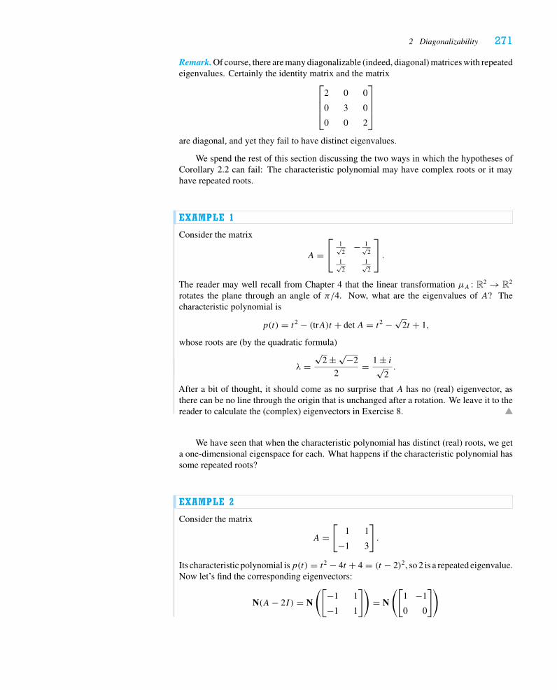
2 Diagonalizability 271
Remark. Of course, there are many diagonalizable (indeed, diagonal) matrices with repeatedeigenvalues. Certainly the identity matrix and the matrix
⎡⎢⎢⎣
2 0 0
0 3 0
0 0 2
⎤⎥⎥⎦
are diagonal, and yet they fail to have distinct eigenvalues.
We spend the rest of this section discussing the two ways in which the hypotheses ofCorollary 2.2 can fail: The characteristic polynomial may have complex roots or it mayhave repeated roots.
EXAMPLE 1
Consider the matrix
A =⎡⎣
1√2
− 1√2
1√2
1√2
⎤⎦ .
The reader may well recall from Chapter 4 that the linear transformation μA : R2 → R2
rotates the plane through an angle of π/4. Now, what are the eigenvalues of A? Thecharacteristic polynomial is
p(t) = t2 − (trA)t + detA = t2 − √2t + 1,
whose roots are (by the quadratic formula)
λ =√
2 ± √−2
2= 1 ± i√
2.
After a bit of thought, it should come as no surprise that A has no (real) eigenvector, asthere can be no line through the origin that is unchanged after a rotation. We leave it to thereader to calculate the (complex) eigenvectors in Exercise 8.
We have seen that when the characteristic polynomial has distinct (real) roots, we geta one-dimensional eigenspace for each. What happens if the characteristic polynomial hassome repeated roots?
EXAMPLE 2
Consider the matrix
A =[
1 1
−1 3
].
Its characteristic polynomial isp(t) = t2 − 4t + 4 = (t − 2)2, so 2 is a repeated eigenvalue.Now let’s find the corresponding eigenvectors:
N(A− 2I ) = N
([−1 1
−1 1
])= N
([1 −1
0 0
])
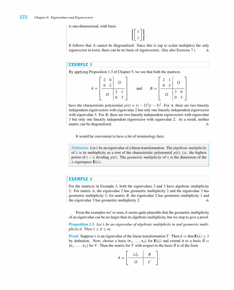
272 Chapter 6 Eigenvalues and Eigenvectors
is one-dimensional, with basis {[1
1
]}.
It follows that A cannot be diagonalized: Since this is (up to scalar multiples) the onlyeigenvector in town, there can be no basis of eigenvectors. (See also Exercise 7.)
EXAMPLE 3
By applying Proposition 1.3 of Chapter 5, we see that both the matrices
A =
⎡⎢⎢⎢⎢⎣
2 0O
0 2
3 1O
0 3
⎤⎥⎥⎥⎥⎦
and B =
⎡⎢⎢⎢⎢⎣
2 1O
0 2
3 0O
0 3
⎤⎥⎥⎥⎥⎦
have the characteristic polynomial p(t) = (t − 2)2(t − 3)2. For A, there are two linearlyindependent eigenvectors with eigenvalue 2 but only one linearly independent eigenvectorwith eigenvalue 3. For B, there are two linearly independent eigenvectors with eigenvalue3 but only one linearly independent eigenvector with eigenvalue 2. As a result, neithermatrix can be diagonalized.
It would be convenient to have a bit of terminology here.
Definition. Let λ be an eigenvalue of a linear transformation. The algebraic multiplicityof λ is its multiplicity as a root of the characteristic polynomial p(t), i.e., the highestpower of t − λ dividing p(t). The geometric multiplicity of λ is the dimension of theλ-eigenspace E(λ).
EXAMPLE 4
For the matrices in Example 3, both the eigenvalues 2 and 3 have algebraic multiplicity2. For matrix A, the eigenvalue 2 has geometric multiplicity 2 and the eigenvalue 3 hasgeometric multiplicity 1; for matrix B, the eigenvalue 2 has geometric multiplicity 1 andthe eigenvalue 3 has geometric multiplicity 2.
From the examples we’ve seen, it seems quite plausible that the geometric multiplicityof an eigenvalue can be no larger than its algebraic multiplicity, but we stop to give a proof.
Proposition 2.3. Let λ be an eigenvalue of algebraic multiplicity m and geometric multi-plicity d . Then 1 ≤ d ≤ m.
Proof. Suppose λ is an eigenvalue of the linear transformation T . Then d = dim E(λ) ≥ 1by definition. Now, choose a basis {v1, . . . , vd} for E(λ) and extend it to a basis B ={v1, . . . , vn} for V . Then the matrix for T with respect to the basis B is of the form
A =⎡⎣ λId B
O C
⎤⎦ ,
2 Diagonalizability 273
and so, by part a of Exercise 5.1.9, the characteristic polynomial
pA(t) = det(A− tI ) = det((λ− t)Id
)det(C − tI ) = (λ− t)d det(C − tI ).
Since the characteristic polynomial does not depend on the basis, and since (t − λ)m is thelargest power of t − λ dividing the characteristic polynomial, it follows that d ≤ m.
We are now able to give a necessary and sufficient criterion for a linear transformationto be diagonalizable. Based on our experience with examples, it should come as no greatsurprise.
Theorem 2.4. Let T : V → V be a linear transformation. Let its distinct eigenvalues beλ1, . . . , λk and assume these are all real numbers. Then T is diagonalizable if and only ifthe geometric multiplicity, di , of each λi equals its algebraic multiplicity, mi .
Proof. Let V be an n-dimensional vector space. Then the characteristic polynomial of Thas degree n, and we have
p(t) = ±(t − λ1)m1(t − λ2)
m2 · · · (t − λk)mk ;therefore,
n =k∑i=1
mi.
Now, suppose T is diagonalizable. Then there is a basis B consisting of eigenvectors.
At most di of these basis vectors lie in E(λi), and so n ≤k∑i=1di . On the other hand, by
Proposition 2.3, we know that di ≤ mi for i = 1, . . . , k. Putting these together, we have
n ≤k∑i=1
di ≤k∑i=1
mi = n.
Thus, there must be equality at each stage here, which implies that di = mi for all i =1, . . . , k.
Conversely, suppose di = mi for i = 1, . . . , k. If we choose a basis Bi for eacheigenspace E(λi) and let B = B1 ∪ · · · ∪ Bk , then we assert that B is a basis for V . Thereare n vectors in B, so we need only check that the set of vectors is linearly indepen-dent. This is a generalization of the argument of Theorem 2.1, and we leave it to Exer-cise 20.
EXAMPLE 5
The matrices
A =
⎡⎢⎢⎣
−1 4 2
−1 3 1
−1 2 2
⎤⎥⎥⎦ and B =
⎡⎢⎢⎣
0 3 1
−1 3 1
0 1 1
⎤⎥⎥⎦
both have characteristic polynomial p(t) = −(t − 1)2(t − 2). That is, the eigenvalue 1has algebraic multiplicity 2 and the eigenvalue 2 has algebraic multiplicity 1. To decidewhether the matrices are diagonalizable, we need to know the geometric multiplicity of the
274 Chapter 6 Eigenvalues and Eigenvectors
eigenvalue 1. Well,
A− I =
⎡⎢⎢⎣
−2 4 2
−1 2 1
−1 2 1
⎤⎥⎥⎦�
⎡⎢⎢⎣
1 −2 −1
0 0 0
0 0 0
⎤⎥⎥⎦
has rank 1 and so dim EA(1) = 2. We infer from Theorem 2.4 that A is diagonalizable.Indeed, as the reader can check, a diagonalizing basis is
⎧⎪⎪⎨⎪⎪⎩
⎡⎢⎢⎣
1
0
1
⎤⎥⎥⎦ ,
⎡⎢⎢⎣
1
1
−1
⎤⎥⎥⎦ ,
⎡⎢⎢⎣
2
1
1
⎤⎥⎥⎦
⎫⎪⎪⎬⎪⎪⎭.
On the other hand,
B − I =
⎡⎢⎢⎣
−1 3 1
−1 2 1
0 1 0
⎤⎥⎥⎦�
⎡⎢⎢⎣
1 0 −1
0 1 0
0 0 0
⎤⎥⎥⎦
has rank 2 and so dim EB(1) = 1. Since the eigenvalue 1 has geometric multiplicity 1, itfollows from Theorem 2.4 that B is not diagonalizable.
In the next section we will see the power of diagonalizing matrices in several appli-cations.
Exercises 6.2
1.∗ Decide whether each of the matrices in Exercise 6.1.1 is diagonalizable. Give yourreasoning.
2. Prove or give a counterexample:a. If A is an n× n matrix with n distinct (real) eigenvalues, then A is diagonalizable.
b. If A is diagonalizable and AB = BA, then B is diagonalizable.
c. If there is an invertible matrix P so that A = P−1BP , then A and B have the sameeigenvalues.
d. If A and B have the same eigenvalues, then there is an invertible matrix P so thatA = P−1BP .
e. There is no real 2 × 2 matrix A satisfying A2 = −I .
f. IfA andB are diagonalizable and have the same eigenvalues (with the same algebraicmultiplicities), then there is an invertible matrix P so that A = P−1BP .
3. Suppose A is a 2 × 2 matrix whose eigenvalues are integers. If detA = 120, explainwhy A must be diagonalizable.
4.∗ Consider the differentiation operator D : Pk → Pk . Is it diagonalizable?
5. Let f1(t) = et , f2(t) = tet , f3(t) = t2et , and let V = Span (f1, f2, f3) ⊂ C∞(R). LetT : V → V be given by T (f ) = f ′′ − 2f ′ + f . Decide whether T is diagonalizable.
6. Is the linear transformation T : Mn×n → Mn×n defined by T (X) = XT diagonaliz-able? (See Exercise 6.1.12; Exercises 2.5.22 and 3.6.8 may also be relevant.)
2 Diagonalizability 275
7.∗ Let A =[
1 1
−1 3
]. We saw in Example 2 that A has repeated eigenvalue 2 and
v1 =[
1
1
]spans E(2).
a. Calculate (A− 2I )2.
b. Solve (A− 2I )v2 = v1 for v2. Explain how we know a priori that this equationhas a solution.
c. Give the matrix for A with respect to the basis {v1, v2}.This is the closest to diagonal one can get and is called the Jordan canonical form ofA. We’ll explore this thoroughly in Section 1 of Chapter 7.
8.∗ Calculate the (complex) eigenvalues and (complex) eigenvectors of the rotation matrix
Aθ =[
cos θ − sin θ
sin θ cos θ
].
9. Prove that if λ is an eigenvalue of A with geometric multiplicity d, then λ is aneigenvalue of AT with geometric multiplicity d. (Hint: Use Theorem 4.6 of Chap-ter 3.)
10. Here you are asked to complete a different proof of Theorem 2.1.a. Show first that {v1, v2} is linearly independent. Suppose c1v1 + c2v2 = 0, and applyT − λ2I to this equation. Use the fact that λ1 �= λ2 to deduce c1 = 0 and, hence,that c2 = 0.
b. Show next that {v1, v2, v3} is linearly independent. (Proceed as in part a, applyingT − λ3I to the equation.)
c. Continue.
11. Suppose A is an n× n matrix with the property that A2 = A.a. Show that if λ is an eigenvalue of A, then λ = 0 or λ = 1.
b. Prove that A is diagonalizable. (Hint: See Exercise 3.2.13.)
12. Suppose A is an n× n matrix with the property that A2 = I .a. Show that if λ is an eigenvalue of A, then λ = 1 or λ = −1.
b. Prove that
E(1) = {x ∈ Rn : x = 12 (u + Au) for some u ∈ Rn} and
E(−1) = {x ∈ Rn : x = 12 (u − Au) for some u ∈ Rn}.
c. Prove that E(1)+ E(−1) = Rn and deduce that A is diagonalizable.(For an application, see Exercise 6 and Exercise 3.6.8.)
13. Suppose A is diagonalizable, and let pA(t) denote the characteristic polynomial of A.Show that pA(A) = O. This result is a special case of the Cayley-Hamilton Theorem.
14. This problem gives a generalization of Exercises 11 and 12 for those readers who recallthe technique of partial fraction decomposition from their calculus class. Supposeλ1, . . . , λk ∈ R are distinct and f (t) = (t − λ1)(t − λ2) · · · (t − λk). Suppose A isan n× n matrix that satisfies the equation f (A) = O. We want to show that A isdiagonalizable.a. By considering the partial fractions decomposition
1
f (t)= c1
t − λ1+ · · · + ck
t − λk ,
show that there are polynomials f1(t), . . . , fk(t) satisfying 1 =k∑j=1fj (t) and
276 Chapter 6 Eigenvalues and Eigenvectors
(t − λj )fj (t)= cjf (t) for j = 1, . . . , k. Conclude that we can write I =k∑j=1fj (A),
where (A− λj I )fj (A) = O for j = 1, . . . , k.
b. Show that every x ∈ Rn can be decomposed as a sum of vectors x = x1 + · · · + xk ,where xj ∈ E(λj ) for j = 1, . . . , k. (Hint: Use the result of part a.)
c. Deduce that A is diagonalizable.
15. LetA be an n× nmatrix all of whose eigenvalues are real numbers. Prove that there isa basis for Rn with respect to which the matrix for A becomes upper triangular. (Hint:Consider a basis {v1, v′
2, . . . , v′n}, where v1 is an eigenvector. Then repeat the argument
with a smaller matrix.)
16. Let A be an orthogonal 3 × 3 matrix.a. Prove that the characteristic polynomial p(t) has a real root.
b. Prove that ‖Ax‖ = ‖x‖ for all x ∈ R3 and deduce that only 1 and −1 can be (real)eigenvalues of A.
c. Prove that if detA = 1, then 1 must be an eigenvalue of A.
d. Prove that if detA = 1 andA �= I , then μA : R3 → R3 is given by rotation throughsome angle θ about some axis. (Hint: First show dim E(1) = 1. Then show thatμA maps E(1)⊥ to itself and use Exercise 2.5.19.)
e. (See the remark on p. 218.) Prove that the composition of rotations in R3 is again arotation.
17. We say an n× n matrix N is nilpotent if Nr = O for some positive integer r .a. Show that 0 is the only eigenvalue of N .
b. Suppose Nn = O and Nn−1 �= O. Prove that there is a basis {v1, . . . , vn} for Rn
with respect to which the matrix for N becomes⎡⎢⎢⎢⎢⎢⎢⎢⎣
0 1
0 1. . .
. . .
0 1
0
⎤⎥⎥⎥⎥⎥⎥⎥⎦.
(Hint: Choose v1 �= 0 in C(Nn−1), and then define v2, . . . , vn appropriately to endup with this matrix representation. To argue that {v1, . . . , vn} is linearly independent,you might want to mimic the proof of Theorem 2.1.)
18. Suppose T : V → V is a linear transformation. Suppose T is diagonalizable (i.e., thereis a basis for V consisting of eigenvectors of T ). Suppose, moreover, that there is asubspaceW ⊂ V with the property that T (W) ⊂ W . Prove that there is a basis forWconsisting of eigenvectors of T . (Hint: Using Exercise 3.4.17, concoct a basis for Vby starting with a basis for W . Consider the matrix for T with respect to this basis.What is its characteristic polynomial?)
19. Suppose A and B are n× n matrices.a. Suppose that both A and B are diagonalizable and that they have the same eigen-
vectors. Prove that AB = BA.
b. Suppose A has n distinct eigenvalues and AB = BA. Prove that every eigenvectorof A is also an eigenvector of B. Conclude that B is diagonalizable. (Query: Needevery eigenvector of B be an eigenvector of A?)
c. Suppose A and B are diagonalizable and AB = BA. Prove that A and B aresimultaneously diagonalizable; i.e., there is a nonsingular matrix P so that bothP−1AP and P−1BP are diagonal. (Hint: If E(λ) is the λ-eigenspace for A, showthat if v ∈ E(λ), then B(v) ∈ E(λ). Now use Exercise 18.)
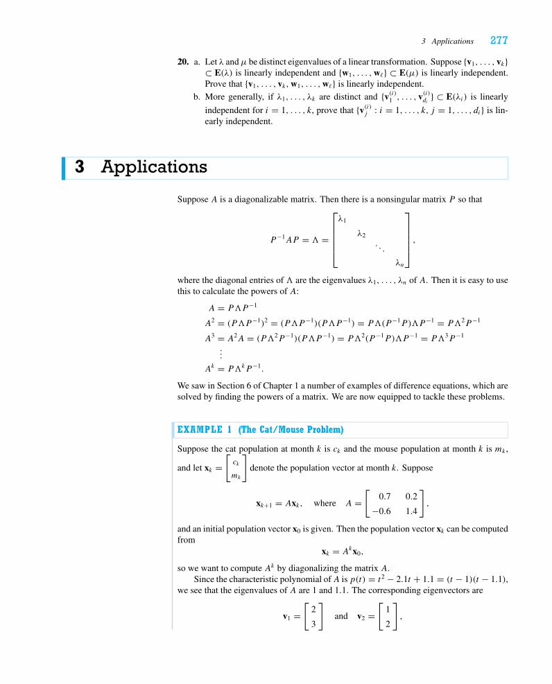
3 Applications 277
20.∗ a. Let λ andμ be distinct eigenvalues of a linear transformation. Suppose {v1, . . . , vk}⊂ E(λ) is linearly independent and {w1, . . . ,w�} ⊂ E(μ) is linearly independent.Prove that {v1, . . . , vk,w1, . . . ,w�} is linearly independent.
b. More generally, if λ1, . . . , λk are distinct and {v(i)1 , . . . , v(i)di
} ⊂ E(λi) is linearly
independent for i = 1, . . . , k, prove that {v(i)j : i = 1, . . . , k, j = 1, . . . , di} is lin-early independent.
3 Applications
Suppose A is a diagonalizable matrix. Then there is a nonsingular matrix P so that
P−1AP = � =
⎡⎢⎢⎢⎢⎣
λ1
λ2. . .
λn
⎤⎥⎥⎥⎥⎦,
where the diagonal entries of � are the eigenvalues λ1, . . . , λn of A. Then it is easy to usethis to calculate the powers of A:
A = P�P−1
A2 = (P�P−1)2 = (P�P−1)(P�P−1) = P�(P−1P)�P−1 = P�2P−1
A3 = A2A = (P�2P−1)(P�P−1) = P�2(P−1P)�P−1 = P�3P−1
...
Ak = P�kP−1.
We saw in Section 6 of Chapter 1 a number of examples of difference equations, which aresolved by finding the powers of a matrix. We are now equipped to tackle these problems.
EXAMPLE 1 (The Cat/Mouse Problem)
Suppose the cat population at month k is ck and the mouse population at month k is mk ,
and let xk =[ck
mk
]denote the population vector at month k. Suppose
xk+1 = Axk, where A =[
0.7 0.2
−0.6 1.4
],
and an initial population vector x0 is given. Then the population vector xk can be computedfrom
xk = Akx0,
so we want to compute Ak by diagonalizing the matrix A.Since the characteristic polynomial ofA is p(t) = t2 − 2.1t + 1.1 = (t − 1)(t − 1.1),
we see that the eigenvalues of A are 1 and 1.1. The corresponding eigenvectors are
v1 =[
2
3
]and v2 =
[1
2
],
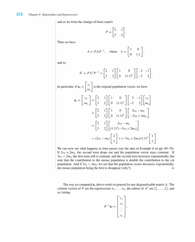
278 Chapter 6 Eigenvalues and Eigenvectors
and so we form the change-of-basis matrix
P =[
2 1
3 2
].
Then we have
A = P�P−1, where � =[
1 0
0 1.1
],
and so
Ak = P�kP−1 =[
2 1
3 2
][1 0
0 (1.1)k
][2 −1
−3 2
].
In particular, if x0 =[c0
m0
]is the original population vector, we have
xk =[ck
mk
]=[
2 1
3 2
][1 0
0 (1.1)k
][2 −1
−3 2
][c0
m0
]
=[
2 1
3 2
][1 0
0 (1.1)k
][2c0 −m0
−3c0 + 2m0
]
=[
2 1
3 2
][2c0 −m0
(1.1)k(−3c0 + 2m0)
]
= (2c0 −m0)
[2
3
]+ (−3c0 + 2m0)(1.1)
k
[1
2
].
We can now see what happens as time passes (see the data in Example 6 on pp. 69–70).If 3c0 = 2m0, the second term drops out and the population vector stays constant. If3c0 < 2m0, the first term still is constant, and the second term increases exponentially, butnote that the contribution to the mouse population is double the contribution to the catpopulation. And if 3c0 > 2m0, we see that the population vector decreases exponentially,the mouse population being the first to disappear (why?).
The way we computed xk above works in general for any diagonalizable matrixA. Thecolumn vectors of P are the eigenvectors v1, . . . , vn, the entries of �k are λk1, . . . , λ
kn, and
so, letting
P−1x0 =
⎡⎢⎢⎢⎢⎢⎣
c1
c2
...
cn
⎤⎥⎥⎥⎥⎥⎦,
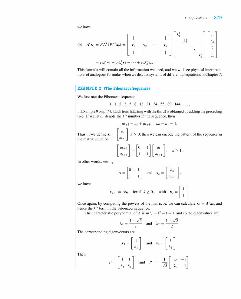
3 Applications 279
we have
Akx0 = P�k(P−1x0) =
⎡⎢⎢⎢⎣
|v1
|
|v2
|· · ·
|vn
|
⎤⎥⎥⎥⎦
⎡⎢⎢⎢⎢⎢⎣
λk1
λk2. . .
λkn
⎤⎥⎥⎥⎥⎥⎦
⎡⎢⎢⎢⎢⎢⎣
c1
c2
...
cn
⎤⎥⎥⎥⎥⎥⎦
(∗)
= c1λk1v1 + c2λ
k2v2 + · · · + cnλknvn.
This formula will contain all the information we need, and we will see physical interpreta-tions of analogous formulas when we discuss systems of differential equations in Chapter 7.
EXAMPLE 2 (The Fibonacci Sequence)
We first met the Fibonacci sequence,
1, 1, 2, 3, 5, 8, 13, 21, 34, 55, 89, 144, . . . ,
in Example 9 on p. 74. Each term (starting with the third) is obtained by adding the precedingtwo: If we let ak denote the kth number in the sequence, then
ak+2 = ak + ak+1, a0 = a1 = 1.
Thus, if we define xk =[ak
ak+1
], k ≥ 0, then we can encode the pattern of the sequence in
the matrix equation[ak+1
ak+2
]=[
0 1
1 1
][ak
ak+1
], k ≥ 1.
In other words, setting
A =[
0 1
1 1
]and xk =
[ak
ak+1
],
we have
xk+1 = Axk for all k ≥ 0, with x0 =[
1
1
].
Once again, by computing the powers of the matrix A, we can calculate xk = Akx0, andhence the kth term in the Fibonacci sequence.
The characteristic polynomial of A is p(t) = t2 − t − 1, and so the eigenvalues are
λ1 = 1 − √5
2and λ2 = 1 + √
5
2.
The corresponding eigenvectors are
v1 =[
1
λ1
]and v2 =
[1
λ2
].
Then
P =[
1 1
λ1 λ2
]and P−1 = 1√
5
[λ2 −1
−λ1 1
],
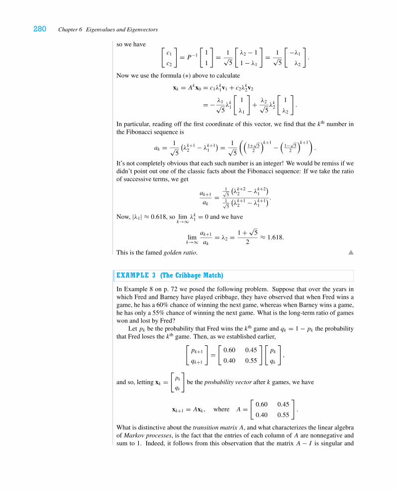
280 Chapter 6 Eigenvalues and Eigenvectors
so we have [c1
c2
]= P−1
[1
1
]= 1√
5
[λ2 − 1
1 − λ1
]= 1√
5
[−λ1
λ2
].
Now we use the formula (∗) above to calculate
xk = Akx0 = c1λk1v1 + c2λ
k2v2
= − λ1√5λk1
[1
λ1
]+ λ2√
5λk2
[1
λ2
].
In particular, reading off the first coordinate of this vector, we find that the kth number inthe Fibonacci sequence is
ak = 1√5
(λk+1
2 − λk+11
) = 1√5
((1+√
52
)k+1 −(
1−√5
2
)k+1).
It’s not completely obvious that each such number is an integer! We would be remiss if wedidn’t point out one of the classic facts about the Fibonacci sequence: If we take the ratioof successive terms, we get
ak+1
ak=
1√5
(λk+2
2 − λk+21
)1√5
(λk+1
2 − λk+11
) .
Now, |λ1| ≈ 0.618, so limk→∞ λ
k1 = 0 and we have
limk→∞
ak+1
ak= λ2 = 1 + √
5
2≈ 1.618.
This is the famed golden ratio.
EXAMPLE 3 (The Cribbage Match)
In Example 8 on p. 72 we posed the following problem. Suppose that over the years inwhich Fred and Barney have played cribbage, they have observed that when Fred wins agame, he has a 60% chance of winning the next game, whereas when Barney wins a game,he has only a 55% chance of winning the next game. What is the long-term ratio of gameswon and lost by Fred?
Let pk be the probability that Fred wins the kth game and qk = 1 − pk the probabilitythat Fred loses the kth game. Then, as we established earlier,
[pk+1
qk+1
]=[
0.60 0.45
0.40 0.55
][pk
qk
],
and so, letting xk =[pk
qk
]be the probability vector after k games, we have
xk+1 = Axk, where A =[
0.60 0.45
0.40 0.55
].
What is distinctive about the transition matrix A, and what characterizes the linear algebraof Markov processes, is the fact that the entries of each column of A are nonnegative andsum to 1. Indeed, it follows from this observation that the matrix A− I is singular and
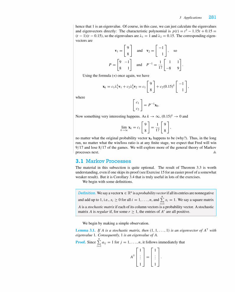
3 Applications 281
hence that 1 is an eigenvalue. Of course, in this case, we can just calculate the eigenvaluesand eigenvectors directly: The characteristic polynomial is p(t) = t2 − 1.15t + 0.15 =(t − 1)(t − 0.15), so the eigenvalues are λ1 = 1 and λ2 = 0.15. The corresponding eigen-vectors are
v1 =[
9
8
]and v2 =
[−1
1
], so
P =[
9 −1
8 1
]and P−1 = 1
17
[1 1
−8 9
].
Using the formula (∗) once again, we have
xk = c1λk1v1 + c2λ
k2v2 = c1
[9
8
]+ c2(0.15)k
[−1
1
],
where [c1
c2
]= P−1x0.
Now something very interesting happens. As k → ∞, (0.15)k → 0 and
limk→∞ xk = c1
[9
8
]= 1
17
[9
8
],
no matter what the original probability vector x0 happens to be (why?). Thus, in the longrun, no matter what the win/loss ratio is at any finite stage, we expect that Fred will win9/17 and lose 8/17 of the games. We will explore more of the general theory of Markovprocesses next.
3.1 Markov ProcessesThe material in this subsection is quite optional. The result of Theorem 3.3 is worthunderstanding, even if one skips its proof (see Exercise 15 for an easier proof of a somewhatweaker result). But it is Corollary 3.4 that is truly useful in lots of the exercises.
We begin with some definitions.
Definition.We say a vector x ∈ Rn is a probability vector if all its entries are nonnegative
and add up to 1, i.e., xi ≥ 0 for all i = 1, . . . , n, andn∑i=1xi = 1. We say a square matrix
A is a stochastic matrix if each of its column vectors is a probability vector. A stochasticmatrix A is regular if, for some r ≥ 1, the entries of Ar are all positive.
We begin by making a simple observation.
Lemma 3.1. If A is a stochastic matrix, then (1, 1, . . . , 1) is an eigenvector of AT witheigenvalue 1. Consequently, 1 is an eigenvalue of A.
Proof. Sincen∑i=1aij = 1 for j = 1, . . . , n, it follows immediately that
AT
⎡⎢⎢⎣
1...
1
⎤⎥⎥⎦ =
⎡⎢⎢⎣
1...
1
⎤⎥⎥⎦ .
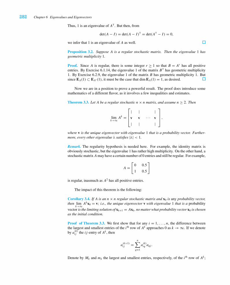
282 Chapter 6 Eigenvalues and Eigenvectors
Thus, 1 is an eigenvalue of AT. But then, from
det(A− I ) = det(A− I )T = det(AT − I ) = 0,
we infer that 1 is an eigenvalue of A as well.
Proposition 3.2. Suppose A is a regular stochastic matrix. Then the eigenvalue 1 hasgeometric multiplicity 1.
Proof. Since A is regular, there is some integer r ≥ 1 so that B = Ar has all positiveentries. By Exercise 6.1.14, the eigenvalue 1 of the matrix BT has geometric multiplicity1. By Exercise 6.2.9, the eigenvalue 1 of the matrix B has geometric multiplicity 1. Butsince EA(1) ⊂ EAr (1), it must be the case that dim EA(1) = 1, as desired.
Now we are in a position to prove a powerful result. The proof does introduce somemathematics of a different flavor, as it involves a few inequalities and estimates.
Theorem 3.3. Let A be a regular stochastic n× n matrix, and assume n ≥ 2. Then
limk→∞A
k =
⎡⎢⎢⎣
|v
|
|v
|· · ·
|v
|
⎤⎥⎥⎦ ,
where v is the unique eigenvector with eigenvalue 1 that is a probability vector. Further-more, every other eigenvalue λ satisfies |λ| < 1.
Remark. The regularity hypothesis is needed here. For example, the identity matrix isobviously stochastic, but the eigenvalue 1 has rather high multiplicity. On the other hand, astochastic matrixAmay have a certain number of 0 entries and still be regular. For example,
A =[
0 0.5
1 0.5
]
is regular, inasmuch as A2 has all positive entries.
The impact of this theorem is the following:
Corollary 3.4. If A is an n× n regular stochastic matrix and x0 is any probability vector,then lim
k→∞Akx0 = v; i.e., the unique eigenvector v with eigenvalue 1 that is a probability
vector is the limiting solution of xk+1 = Axk , no matter what probability vector x0 is chosenas the initial condition.
Proof of Theorem 3.3. We first show that for any i = 1, . . . , n, the difference betweenthe largest and smallest entries of the i th row of Ak approaches 0 as k → ∞. If we denoteby a(k)ij the ij -entry of Ak , then
a(k+1)ij =
n∑q=1
a(k)iq aqj .
Denote by Mk and mk the largest and smallest entries, respectively, of the i th row of Ak;
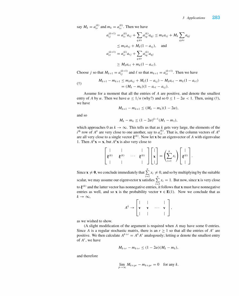
3 Applications 283
sayMk = a(k)ir and mk = a
(k)is . Then we have
a(k+1)ij = a
(k)is asj +
∑q �=sa(k)iq aqj ≤ mkasj +Mk
∑q �=saqj
≤ mkasj +Mk(1 − asj ), and
a(k+1)i� = a
(k)ir arj +
∑q �=r
a(k)iq aqj
≥ Mkar� +mk(1 − ar�).Choose j so thatMk+1 = a
(k+1)ij and � so that mk+1 = a
(k+1)i� . Then we have
Mk+1 −mk+1 ≤ mkasj +Mk(1 − asj )−Mkar� −mk(1 − ar�)= (Mk −mk)(1 − ar� − asj ).(†)
Assume for a moment that all the entries of A are positive, and denote the smallestentry of A by α. Then we have α ≤ 1/n (why?) and so 0 ≤ 1 − 2α < 1. Then, using (†),we have
Mk+1 −mk+1 ≤ (Mk −mk)(1 − 2α),
and soMk −mk ≤ (1 − 2α)k−1(M1 −m1),
which approaches 0 as k → ∞. This tells us that as k gets very large, the elements of thei th row of Ak are very close to one another, say to a(k)i1 . That is, the column vectors of Ak
are all very close to a single vector ξ (k). Now let x be an eigenvector of A with eigenvalue1. Then Akx = x, but Akx is also very close to
⎡⎢⎣
|ξ (k)
|
|ξ (k)
|· · ·
|ξ (k)
|
⎤⎥⎦
⎡⎢⎣
|x|
⎤⎥⎦ =
(n∑i=1
xi
)⎡⎢⎣
|ξ (k)
|
⎤⎥⎦ .
Since x �= 0, we conclude immediately thatn∑i=1xi �= 0, and so by multiplying by the suitable
scalar, we may assume our eigenvector x satisfiesn∑i=1xi = 1. But now, since x is very close
to ξ (k) and the latter vector has nonnegative entries, it follows that x must have nonnegativeentries as well, and so x is the probability vector v ∈ E(1). Now we conclude that ask → ∞,
Ak →⎡⎢⎣
|v|
|v|
· · ·|v|
⎤⎥⎦ ,
as we wished to show.(A slight modification of the argument is required when A may have some 0 entries.
Since A is a regular stochastic matrix, there is an r ≥ 1 so that all the entries of Ar arepositive. We then calculate Ak+r = AkAr analogously; letting α denote the smallest entryof Ar , we have
Mk+r −mk+r ≤ (1 − 2α)(Mk −mk),and therefore
limp→∞Mk+pr −mk+pr = 0 for any k.
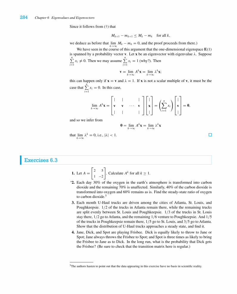
284 Chapter 6 Eigenvalues and Eigenvectors
Since it follows from (†) that
Mk+1 −mk+1 ≤ Mk −mk for all k,
we deduce as before that limk→∞Mk −mk = 0, and the proof proceeds from there.)
We have seen in the course of this argument that the one-dimensional eigenspace E(1)is spanned by a probability vector v. Let x be an eigenvector with eigenvalue λ. Supposen∑i=1xi �= 0. Then we may assume
n∑i=1xi = 1 (why?). Then
v = limk→∞A
kx = limk→∞ λ
kx;this can happen only if x = v and λ = 1. If x is not a scalar multiple of v, it must be the
case thatn∑i=1xi = 0. In this case,
limk→∞A
kx =
⎡⎢⎢⎣
|v
|
|v
|· · ·
|v
|
⎤⎥⎥⎦
⎡⎢⎢⎣
|x
|
⎤⎥⎥⎦ =
(n∑i=1
xi
)⎡⎢⎢⎣|v
|
⎤⎥⎥⎦ = 0,
and so we infer from0 = lim
k→∞Akx = lim
k→∞ λkx
that limk→∞ λ
k = 0, i.e., |λ| < 1.
Exercises 6.3
1. Let A =[
2 5
1 −2
]. Calculate Ak for all k ≥ 1.
2.∗ Each day 30% of the oxygen in the earth’s atmosphere is transformed into carbondioxide and the remaining 70% is unaffected. Similarly, 40% of the carbon dioxide istransformed into oxygen and 60% remains as is. Find the steady-state ratio of oxygento carbon dioxide.5
3. Each month U-Haul trucks are driven among the cities of Atlanta, St. Louis, andPoughkeepsie. 1/2 of the trucks in Atlanta remain there, while the remaining trucksare split evenly between St. Louis and Poughkeepsie. 1/3 of the trucks in St. Louisstay there, 1/2 go to Atlanta, and the remaining 1/6 venture to Poughkeepsie. And 1/5of the trucks in Poughkeepsie remain there, 1/5 go to St. Louis, and 3/5 go to Atlanta.Show that the distribution of U-Haul trucks approaches a steady state, and find it.
4. Jane, Dick, and Spot are playing Frisbee. Dick is equally likely to throw to Jane orSpot; Jane always throws the Frisbee to Spot; and Spot is three times as likely to bringthe Frisbee to Jane as to Dick. In the long run, what is the probability that Dick getsthe Frisbee? (Be sure to check that the transition matrix here is regular.)
5The authors hasten to point out that the data appearing in this exercise have no basis in scientific reality.
3 Applications 285
5.∗ Suppose each of two tubs contains two bottles of beer; two are Budweiser and two areBeck’s. Each minute, Fraternity Freddy picks a bottle of beer from each tub at randomand replaces it in the other tub. After a long time, what portion of the time will therebe exactly one bottle of Beck’s in the first tub? at least one bottle of Beck’s?
6.∗ Gambling Gus has $200 and plays a game where he must continue playing until he haseither lost all his money or doubled it. In each game, he has a 2/5 chance of winning$100 and a 3/5 chance of losing $100. What is the probability that he eventually losesall his money? (Warning: The stochastic matrix here is far from regular, so there is nosteady state. A calculator or computer is required.)
7.∗ If a0 = 2, a1 = 3, and ak+1 = 3ak − 2ak−1, for all k ≥ 1, use methods of linear algebrato determine the formula for ak .
8. If a0 = a1 = 1 and ak+1 = ak + 6ak−1 for all k ≥ 1, use methods of linear algebra todetermine the formula for ak .
9. Suppose a0 = 0, a1 = 1, and ak+1 = 3ak + 4ak−1 for all k ≥ 1. Use methods of linearalgebra to find the formula for ak .
10. If a0 = 0, a1 = 1, and ak+1 = 4ak − 4ak−1 for all k ≥ 1, use methods of linear algebrato determine the formula for ak . (Hint: The matrix will not be diagonalizable, but youcan get close if you stare at Exercise 6.2.7.)
11.∗ If a0 = 0, a1 = a2 = 1, and ak+1 = 2ak + ak−1 − 2ak−2 for k ≥ 2, use methods oflinear algebra to determine the formula for ak .
12. Consider the cat/mouse population problem studied in Example 1. Solve the followingversions, including an investigation of the dependence on the original populations.
a. ck+1 = 0.7ck + 0.1mk
mk+1 = −0.2ck + mk
b.∗ ck+1 = 1.3ck + 0.2mk
mk+1 = −0.1ck + mk
c. ck+1 = 1.1ck + 0.3mk
mk+1 = 0.1ck + 0.9mkWhat conclusions do you draw?
13. Show that when x is a probability vector andA is a stochastic matrix, thenAx is anotherprobability vector.
14. SupposeA is a stochastic matrix and x is an eigenvector with eigenvalue λ �= 1. Showdirectly (i.e., without reference to the proof of Theorem 3.3) that (1, 1, . . . , 1) · x = 0.
15. a. LetA be a stochastic matrix with positive entries, let x ∈ Rn, and let y = Ax. Showthat
|y1| + |y2| + · · · + |yn| ≤ |x1| + |x2| + · · · + |xn|and that equality holds if and only if all the (nonzero) entries of x have the samesign.
b. Show that if A is a stochastic matrix with positive entries and x is an eigenvectorwith eigenvalue 1, then all the entries of x have the same sign.
c. Prove using part b that if A is a stochastic matrix with positive entries, then there isa unique probability vector in E(1) and hence dim E(1) = 1.
d. Prove that if λ is an eigenvalue of a stochastic matrix with positive entries, then|λ| ≤ 1.
e. Assume A is a diagonalizable, regular stochastic matrix. Prove Theorem 3.3.
286 Chapter 6 Eigenvalues and Eigenvectors
4 The Spectral Theorem
We now turn to the study of a large class of diagonalizable matrices, the symmetric matrices.Recall that a square matrix A is symmetric when A = AT. To begin our exploration, let’sstart with a general symmetric 2 × 2 matrix
A =[a b
b c
],
whose characteristic polynomial is p(t) = t2 − (a + c)t + (ac − b2). By the quadraticformula, its eigenvalues are
λ = (a + c)±√(a + c)2 − 4(ac − b2)
2= (a + c)±√(a − c)2 + 4b2
2.
The first thing we notice here is that both eigenvalues are real (because the expression underthe radical is a sum of squares). When A is not diagonal to begin with, b �= 0, and so theeigenvalues of A are necessarily distinct. Thus, in all instances, the symmetric matrix A isdiagonalizable. Moreover, the corresponding eigenvectors are
v1 =[
b
λ1 − a
]and v2 =
[λ2 − cb
];
note thatv1 · v2 = b(λ2 − c)+ (λ1 − a)b = b(λ1 + λ2 − a − c) = 0,
and so the eigenvectors are orthogonal. Since there is an orthogonal basis for R2 consistingof eigenvectors ofA, we of course have an orthonormal basis for R2 consisting of eigenvec-tors of A. That is, by an appropriate rotation of the usual basis, we obtain a diagonalizingbasis for A.
EXAMPLE 1
The eigenvalues of
A =[
1 2
2 −2
]
are λ1 = 2 and λ2 = −3, with corresponding eigenvectors
v1 =[
2
1
]and v2 =
[−1
2
].
By making these vectors unit vectors, we obtain an orthonormal basis
q1 = 1√5
[2
1
], q2 = 1√
5
[−1
2
].
See Figure 4.1.
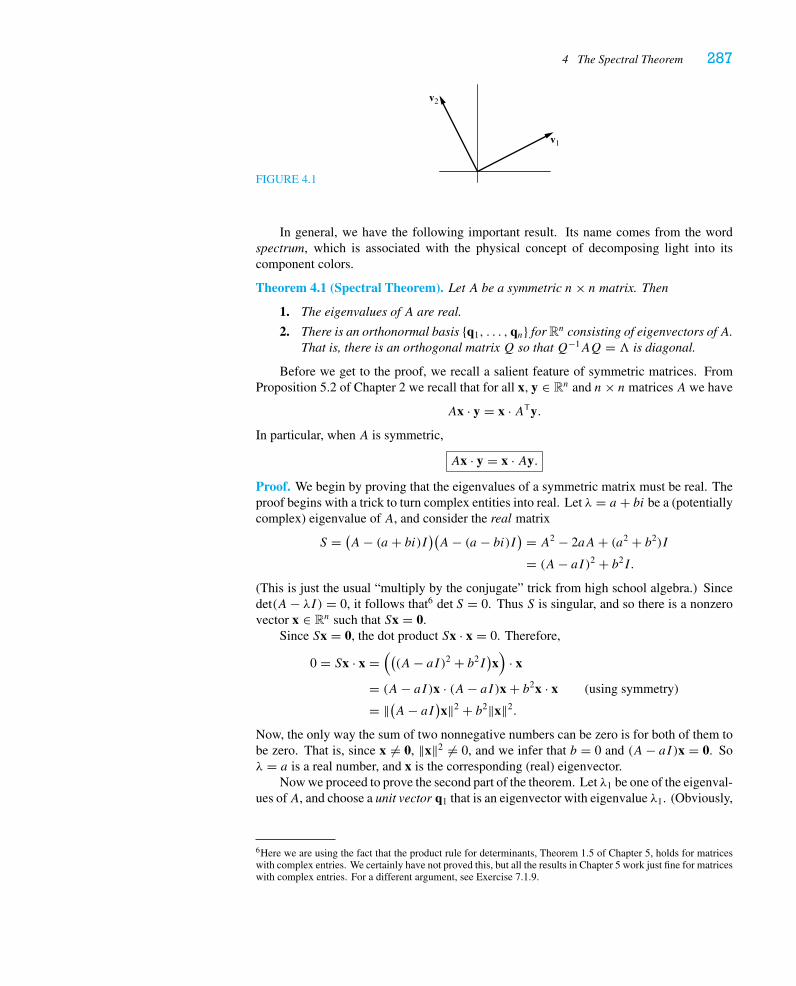
4 The Spectral Theorem 287
FIGURE 4.1
v2
v1
In general, we have the following important result. Its name comes from the wordspectrum, which is associated with the physical concept of decomposing light into itscomponent colors.
Theorem 4.1 (Spectral Theorem). Let A be a symmetric n× n matrix. Then
1. The eigenvalues of A are real.
2. There is an orthonormal basis {q1, . . . ,qn} for Rn consisting of eigenvectors ofA.That is, there is an orthogonal matrixQ so thatQ−1AQ = � is diagonal.
Before we get to the proof, we recall a salient feature of symmetric matrices. FromProposition 5.2 of Chapter 2 we recall that for all x, y ∈ Rn and n× n matrices A we have
Ax · y = x · ATy.
In particular, when A is symmetric,
Ax · y = x · Ay.
Proof. We begin by proving that the eigenvalues of a symmetric matrix must be real. Theproof begins with a trick to turn complex entities into real. Let λ = a + bi be a (potentiallycomplex) eigenvalue of A, and consider the real matrix
S = (A− (a + bi)I)(A− (a − bi)I) = A2 − 2aA+ (a2 + b2)I
= (A− aI)2 + b2I.
(This is just the usual “multiply by the conjugate” trick from high school algebra.) Sincedet(A− λI) = 0, it follows that6 det S = 0. Thus S is singular, and so there is a nonzerovector x ∈ Rn such that Sx = 0.
Since Sx = 0, the dot product Sx · x = 0. Therefore,
0 = Sx · x =(((A− aI)2 + b2I
)x)
· x
= (A− aI)x · (A− aI)x + b2x · x (using symmetry)
= ‖(A− aI)x‖2 + b2‖x‖2.
Now, the only way the sum of two nonnegative numbers can be zero is for both of them tobe zero. That is, since x �= 0, ‖x‖2 �= 0, and we infer that b = 0 and (A− aI)x = 0. Soλ = a is a real number, and x is the corresponding (real) eigenvector.
Now we proceed to prove the second part of the theorem. Let λ1 be one of the eigenval-ues ofA, and choose a unit vector q1 that is an eigenvector with eigenvalue λ1. (Obviously,
6Here we are using the fact that the product rule for determinants, Theorem 1.5 of Chapter 5, holds for matriceswith complex entries. We certainly have not proved this, but all the results in Chapter 5 work just fine for matriceswith complex entries. For a different argument, see Exercise 7.1.9.
288 Chapter 6 Eigenvalues and Eigenvectors
this is no problem. We pick an eigenvector and then make it a unit vector by dividing byits length.) Choose {v2, . . . , vn} to be any orthonormal basis for
(Span (q1)
)⊥. What, then,is the matrix for the linear transformation μA with respect to the new (orthonormal) basis{q1, v2, . . . , vn}? It looks like
B =
⎡⎢⎢⎢⎢⎢⎣
λ1 ∗ · · · ∗0... C
0
⎤⎥⎥⎥⎥⎥⎦,
for some (n− 1)× (n− 1) matrix C and some entries ∗. By the change-of-basis formula,we have
B = Q−1AQ = QTAQ,
becauseQ is an orthogonal matrix. Therefore,
BT = (QTAQ)T = QTATQ = QTAQ = B.
SinceB is symmetric, we deduce that the entries ∗ are all 0 and thatC is likewise symmetric.We now consider the (n− 1)× (n− 1) symmetric matrixC: Aunit length eigenvector ofCin Rn−1 corresponds to a unit vector q2 in the (n− 1)-dimensional subspace
(Span (q1)
)⊥.Continuing this process n− 2 steps further, we arrive at an orthonormal basis {q1, . . . ,qn}consisting of eigenvectors of A.
EXAMPLE 2
Consider the symmetric matrix
A =
⎡⎢⎢⎣
0 1 1
1 1 0
1 0 1
⎤⎥⎥⎦ .
Its characteristic polynomial is p(t) = −t3 + 2t2 + t − 2 = −(t2 − 1)(t − 2) =−(t + 1)(t − 1)(t − 2), so the eigenvalues of A are −1, 1, and 2. As the reader cancheck, the corresponding eigenvectors are
v1 =
⎡⎢⎢⎣
−2
1
1
⎤⎥⎥⎦ , v2 =
⎡⎢⎢⎣
0
−1
1
⎤⎥⎥⎦ , and v3 =
⎡⎢⎢⎣
1
1
1
⎤⎥⎥⎦ .
Note that these three vectors form an orthogonal basis for R3, and we can easily obtain anorthonormal basis by making them unit vectors:
q1 = 1√6
⎡⎢⎢⎣
−2
1
1
⎤⎥⎥⎦ , q2 = 1√
2
⎡⎢⎢⎣
0
−1
1
⎤⎥⎥⎦ , and q3 = 1√
3
⎡⎢⎢⎣
1
1
1
⎤⎥⎥⎦ .
The orthogonal diagonalizing matrixQ is therefore
Q =
⎡⎢⎢⎣
− 2√6
0 1√3
1√6
− 1√2
1√3
1√6
1√2
1√3
⎤⎥⎥⎦ .
4 The Spectral Theorem 289
EXAMPLE 3
Consider the symmetric matrix
A =
⎡⎢⎢⎣
5 −4 −2
−4 5 −2
−2 −2 8
⎤⎥⎥⎦ .
Its characteristic polynomial is p(t) = −t3 + 18t2 − 81t = −t (t − 9)2, so the eigenvaluesof A are 0, 9, and 9. It is easy to check that
v1 =
⎡⎢⎢⎣
2
2
1
⎤⎥⎥⎦
gives a basis for E(0) = N(A). As for E(9), we find
A− 9I =
⎡⎢⎢⎣
−4 −4 −2
−4 −4 −2
−2 −2 −1
⎤⎥⎥⎦ ,
which has rank 1, and so, as the Spectral Theorem guarantees, E(9) is two-dimensional,with basis
v2 =
⎡⎢⎢⎣
−1
1
0
⎤⎥⎥⎦ and v3 =
⎡⎢⎢⎣
−1
0
2
⎤⎥⎥⎦ .
If we want an orthogonal (or orthonormal) basis, we must use the Gram-Schmidt process,Theorem 2.4 of Chapter 4: We take w2 = v2 and let
w3 = v3 − projw2v3 =
⎡⎢⎢⎣
−1
0
2
⎤⎥⎥⎦− 1
2
⎡⎢⎢⎣
−1
1
0
⎤⎥⎥⎦ =
⎡⎢⎢⎣
− 12
− 12
2
⎤⎥⎥⎦ .
It is convenient to eschew fractions, and so we let
w′3 = 2w3 =
⎡⎢⎢⎣
−1
−1
4
⎤⎥⎥⎦ .
As a check, note that v1,w2,w′3 do in fact form an orthogonal basis. As before, if we want
the orthogonal diagonalizing matrix Q, we must make these vectors unit vectors, so wetake
q1 = 1
3
⎡⎢⎢⎣
2
2
1
⎤⎥⎥⎦ , q2 = 1√
2
⎡⎢⎢⎣
−1
1
0
⎤⎥⎥⎦ , and q3 = 1
3√
2
⎡⎢⎢⎣
−1
−1
4
⎤⎥⎥⎦ ,
whence
Q =
⎡⎢⎢⎣
23 − 1√
2− 1
3√
223
1√2
− 13√
213 0 4
3√
2
⎤⎥⎥⎦ .
We reiterate that repeated eigenvalues cause no problem with symmetric matrices.
290 Chapter 6 Eigenvalues and Eigenvectors
We conclude this discussion with a comparison to our study of projections in Chapter4. Note that if we write outA = Q�Q−1 = Q�QT, we see, reasoning as in Exercise 2.5.4,that
A =
⎡⎢⎢⎣
|q1
|
|q2
|· · ·
|qn
|
⎤⎥⎥⎦
⎡⎢⎢⎢⎢⎢⎣
λ1
λ2
. . .
λn
⎤⎥⎥⎥⎥⎥⎦
⎡⎢⎢⎢⎢⎢⎣
qT1
qT2...
qTn
⎤⎥⎥⎥⎥⎥⎦
=n∑i=1
λiqiqTi .
This is the so-called spectral decomposition of A: Multiplying by a symmetric matrix Ais the same as taking a weighted sum (weighted by the eigenvalues) of projections ontothe respective eigenspaces. (See Proposition 2.3 of Chapter 4.) This is, indeed, a beautifulresult with many applications in higher mathematics and physics.
4.1 Conics and Quadric Surfaces: A Brief Respitefrom LinearityWe now use the Spectral Theorem to analyze the equations of conic sections and quadricsurfaces.
EXAMPLE 4
Suppose we are given the quadratic equation
x21 + 4x1x2 − 2x2
2 = 6
to graph. Notice that we can write the quadratic expression
x21 + 4x1x2 − 2x2
2 =[x1 x2
] [1 2
2 −2
][x1
x2
]= xTAx,
where
A =[
1 2
2 −2
]
is the symmetric matrix we analyzed in Example 1 above. Thus, we know that
A = Q�QT, where Q = 1√5
[2 −1
1 2
]and � =
[2 0
0 −3
].
So, if we make the substitution y = QTx, then we have
xTAx = xT(Q�QT)x = (QTx)T�(QTx) = yT�y = 2y21 − 3y2
2 .
Note that the conic is much easier to understand in the y1y2-coordinates. Indeed, werecognize that the equation 2y2
1 − 3y22 = 6 can be written in the form
y21
3− y2
2
2= 1,
from which we see that this is a hyperbola with asymptotes y2 = ±√
23y1, as pictured in
Figure 4.2. Now recall that the y1y2-coordinates are the coordinates with respect to the
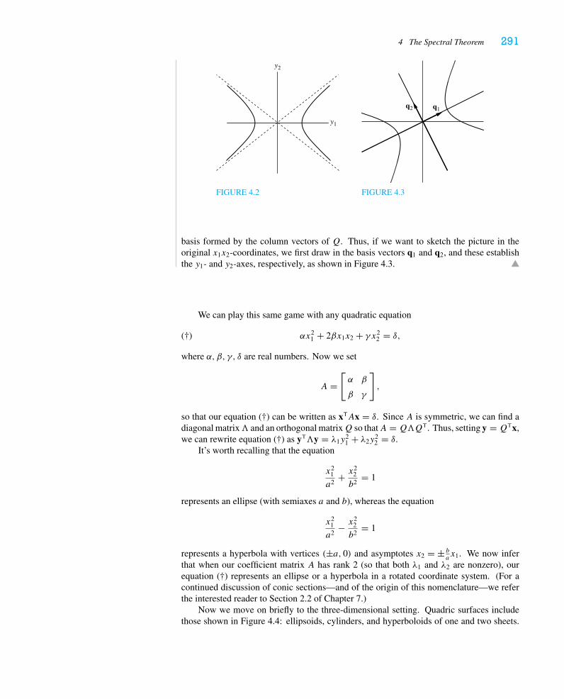
4 The Spectral Theorem 291
y2
y1
FIGURE 4.2
q2 q1
FIGURE 4.3
basis formed by the column vectors of Q. Thus, if we want to sketch the picture in theoriginal x1x2-coordinates, we first draw in the basis vectors q1 and q2, and these establishthe y1- and y2-axes, respectively, as shown in Figure 4.3.
We can play this same game with any quadratic equation
(†) αx21 + 2βx1x2 + γ x2
2 = δ,
where α, β, γ, δ are real numbers. Now we set
A =[α β
β γ
],
so that our equation (†) can be written as xTAx = δ. Since A is symmetric, we can find adiagonal matrix� and an orthogonal matrixQ so thatA = Q�QT. Thus, setting y = QTx,we can rewrite equation (†) as yT�y = λ1y
21 + λ2y
22 = δ.
It’s worth recalling that the equation
x21
a2+ x2
2
b2= 1
represents an ellipse (with semiaxes a and b), whereas the equation
x21
a2− x2
2
b2= 1
represents a hyperbola with vertices (±a, 0) and asymptotes x2 = ± bax1. We now infer
that when our coefficient matrix A has rank 2 (so that both λ1 and λ2 are nonzero), ourequation (†) represents an ellipse or a hyperbola in a rotated coordinate system. (For acontinued discussion of conic sections—and of the origin of this nomenclature—we referthe interested reader to Section 2.2 of Chapter 7.)
Now we move on briefly to the three-dimensional setting. Quadric surfaces includethose shown in Figure 4.4: ellipsoids, cylinders, and hyperboloids of one and two sheets.
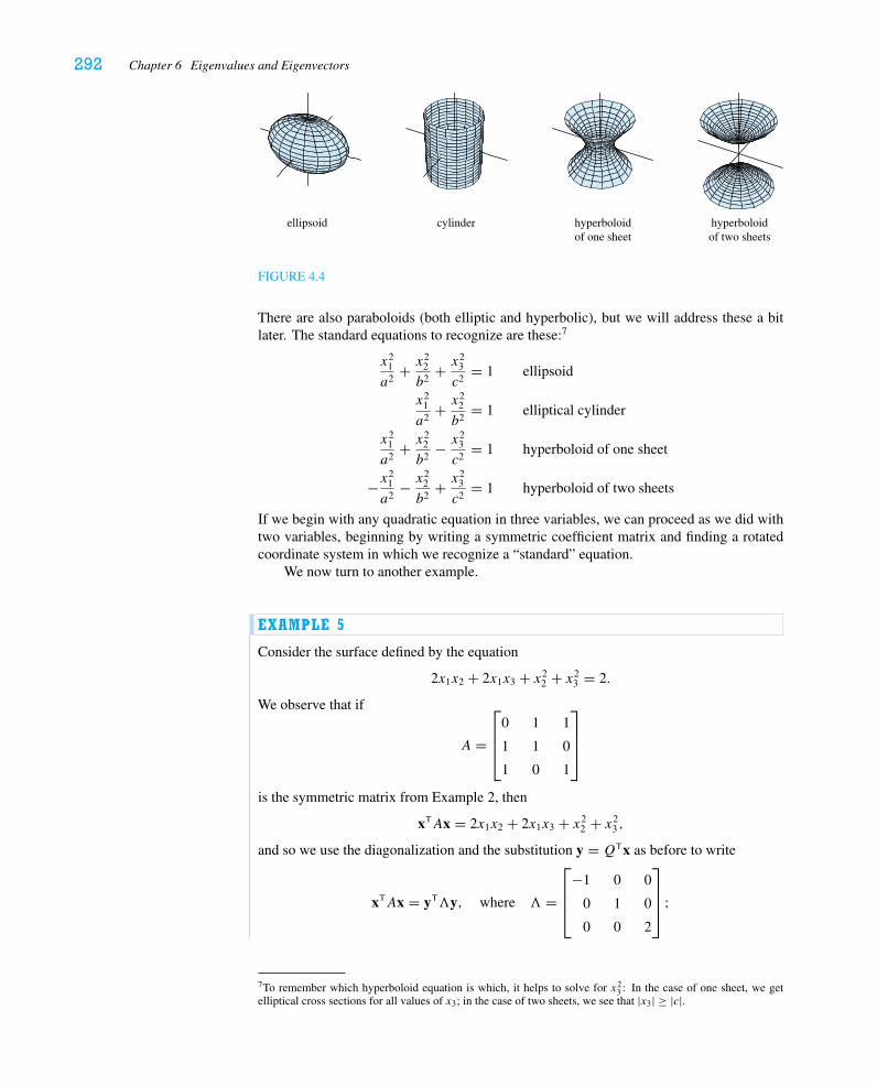
292 Chapter 6 Eigenvalues and Eigenvectors
ellipsoid cylinder hyperboloidof one sheet
hyperboloidof two sheets
FIGURE 4.4
There are also paraboloids (both elliptic and hyperbolic), but we will address these a bitlater. The standard equations to recognize are these:7
x21
a2+ x2
2
b2+ x2
3
c2= 1 ellipsoid
x21
a2+ x2
2
b2= 1 elliptical cylinder
x21
a2+ x2
2
b2− x2
3
c2= 1 hyperboloid of one sheet
−x21
a2− x2
2
b2+ x2
3
c2= 1 hyperboloid of two sheets
If we begin with any quadratic equation in three variables, we can proceed as we did withtwo variables, beginning by writing a symmetric coefficient matrix and finding a rotatedcoordinate system in which we recognize a “standard” equation.
We now turn to another example.
EXAMPLE 5
Consider the surface defined by the equation
2x1x2 + 2x1x3 + x22 + x2
3 = 2.
We observe that if
A =
⎡⎢⎢⎣
0 1 1
1 1 0
1 0 1
⎤⎥⎥⎦
is the symmetric matrix from Example 2, then
xTAx = 2x1x2 + 2x1x3 + x22 + x2
3 ,
and so we use the diagonalization and the substitution y = QTx as before to write
xTAx = yT�y, where � =
⎡⎢⎢⎣
−1 0 0
0 1 0
0 0 2
⎤⎥⎥⎦ ;
7To remember which hyperboloid equation is which, it helps to solve for x23 : In the case of one sheet, we get
elliptical cross sections for all values of x3; in the case of two sheets, we see that |x3| ≥ |c|.
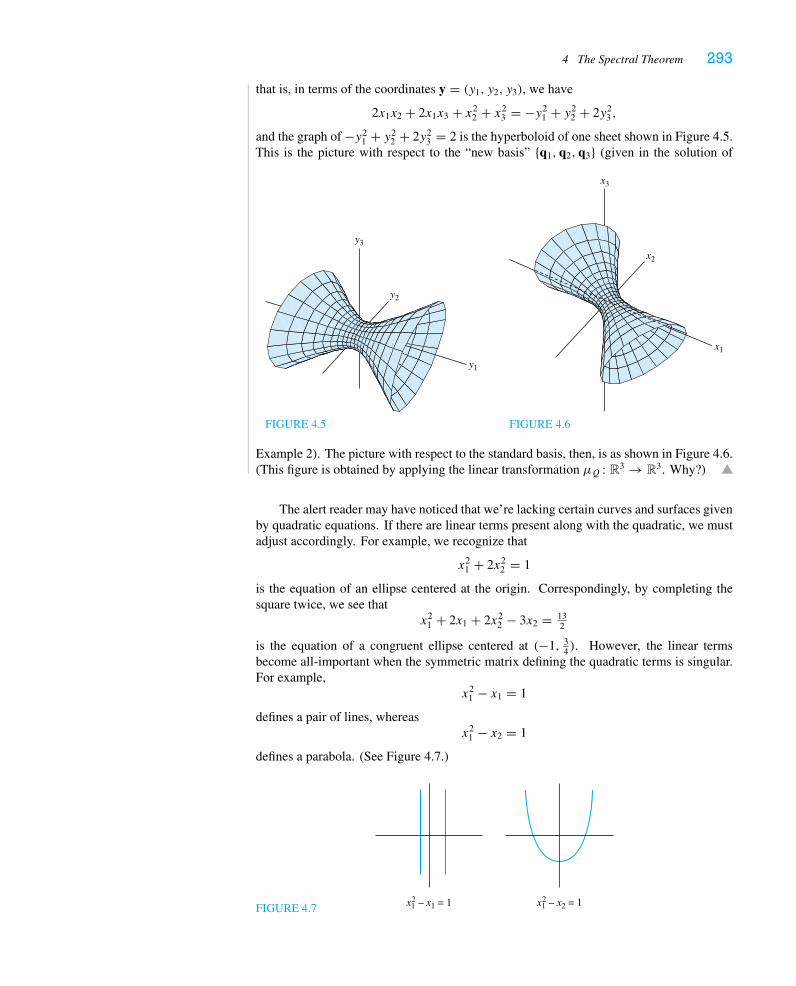
4 The Spectral Theorem 293
that is, in terms of the coordinates y = (y1, y2, y3), we have
2x1x2 + 2x1x3 + x22 + x2
3 = −y21 + y2
2 + 2y23 ,
and the graph of −y21 + y2
2 + 2y23 = 2 is the hyperboloid of one sheet shown in Figure 4.5.
This is the picture with respect to the “new basis” {q1, q2, q3} (given in the solution of
y3
y2
y1
FIGURE 4.5
x3
x1
x2
FIGURE 4.6
Example 2). The picture with respect to the standard basis, then, is as shown in Figure 4.6.(This figure is obtained by applying the linear transformation μQ : R3 → R3. Why?)
The alert reader may have noticed that we’re lacking certain curves and surfaces givenby quadratic equations. If there are linear terms present along with the quadratic, we mustadjust accordingly. For example, we recognize that
x21 + 2x2
2 = 1
is the equation of an ellipse centered at the origin. Correspondingly, by completing thesquare twice, we see that
x21 + 2x1 + 2x2
2 − 3x2 = 132
is the equation of a congruent ellipse centered at (−1, 34 ). However, the linear terms
become all-important when the symmetric matrix defining the quadratic terms is singular.For example,
x21 − x1 = 1
defines a pair of lines, whereasx2
1 − x2 = 1
defines a parabola. (See Figure 4.7.)
FIGURE 4.7 x12 – x1 = 1 x1
2 – x2 = 1
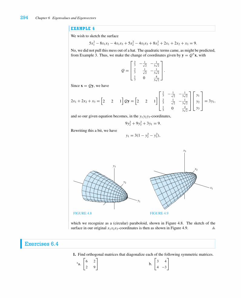
294 Chapter 6 Eigenvalues and Eigenvectors
EXAMPLE 6
We wish to sketch the surface
5x21 − 8x1x2 − 4x1x3 + 5x2
2 − 4x2x3 + 8x23 + 2x1 + 2x2 + x3 = 9.
No, we did not pull this mess out of a hat. The quadratic terms came, as might be predicted,from Example 3. Thus, we make the change of coordinates given by y = QTx, with
Q =
⎡⎢⎢⎣
23 − 1√
2− 1
3√
223
1√2
− 13√
213 0 4
3√
2
⎤⎥⎥⎦ .
Since x = Qy, we have
2x1 + 2x2 + x3 =[2 2 1
]Qy =
[2 2 1
]⎡⎢⎢⎣
23 − 1√
2− 1
3√
223
1√2
− 13√
213 0 4
3√
2
⎤⎥⎥⎦
⎡⎢⎢⎣y1
y2
y3
⎤⎥⎥⎦ = 3y1,
and so our given equation becomes, in the y1y2y3-coordinates,
9y22 + 9y2
3 + 3y1 = 9.
Rewriting this a bit, we havey1 = 3(1 − y2
2 − y23),
y3
y1
y2
FIGURE 4.8
x3
x1
x2
FIGURE 4.9
which we recognize as a (circular) paraboloid, shown in Figure 4.8. The sketch of thesurface in our original x1x2x3-coordinates is then as shown in Figure 4.9.
Exercises 6.4
1. Find orthogonal matrices that diagonalize each of the following symmetric matrices.
a.∗[
6 2
2 9
]b.
[3 4
4 −3
]
4 The Spectral Theorem 295
c.
⎡⎢⎣
2 0 0
0 1 −1
0 −1 1
⎤⎥⎦
d.∗
⎡⎢⎣
2 2 −2
2 −1 −1
−2 −1 −1
⎤⎥⎦
e.∗
⎡⎢⎣
3 2 2
2 2 0
2 0 4
⎤⎥⎦
f.
⎡⎢⎣
1 −2 2
−2 1 2
2 2 1
⎤⎥⎦
g.
⎡⎢⎢⎢⎣
1 0 1 0
0 1 0 1
1 0 1 0
0 1 0 1
⎤⎥⎥⎥⎦
2.∗ Suppose A is a symmetric matrix with eigenvalues 2 and 5. If the vectors
⎡⎢⎣
1
1
−1
⎤⎥⎦ and⎡
⎢⎣1
−1
0
⎤⎥⎦ span the 5-eigenspace, what is A
⎡⎢⎣
1
1
2
⎤⎥⎦? Give your reasoning.
3. A symmetric matrix A has eigenvalues 1 and 2. Find A if
⎡⎢⎣
1
1
1
⎤⎥⎦ spans E(2).
4. Suppose A is symmetric, A
[1
1
]=[
2
2
], and detA = 6. Give the matrix A. Explain
your reasoning clearly. (Hint: What are the eigenvalues of A?)
5. Decide (as efficiently as possible) which of the following matrices are diagonalizable.Give your reasoning.
A =
⎡⎢⎢⎣
5 0 2
0 5 0
0 0 5
⎤⎥⎥⎦ , B =
⎡⎢⎢⎣
5 0 2
0 5 0
2 0 5
⎤⎥⎥⎦ ,
C =
⎡⎢⎢⎣
1 2 4
0 2 2
0 0 3
⎤⎥⎥⎦ , D =
⎡⎢⎢⎣
1 2 4
0 2 2
0 0 1
⎤⎥⎥⎦ .
6. LetA be a symmetric matrix. Without using the Spectral Theorem, show that if λ �= μ,x ∈ E(λ), and y ∈ E(μ), then x · y = 0.
7.∗ Show that if λ is the only eigenvalue of a symmetric matrix A, then A = λI .
8. Suppose A is a diagonalizable matrix whose eigenspaces are orthogonal. Prove that Ais symmetric.
9. a. Suppose A is a symmetric n× n matrix. Using the Spectral Theorem, prove that ifAx · x = 0 for every vector x ∈ Rn, then A = O.
b. Give an example to show that the hypothesis of symmetry is needed in part a.
10. Apply the Spectral Theorem to establish that any symmetric matrixA satisfyingA2 = A
is in fact a projection matrix.
11. a. Suppose A is a symmetric n× n matrix satisfying A4 = I . Use the Spectral Theo-rem to give a complete description of μA : Rn → Rn. (Hint: For starters, what arethe potential eigenvalues of A?)
b. What happens for a symmetric n× n matrix satisfying Ak = I for some integerk ≥ 2?
296 Chapter 6 Eigenvalues and Eigenvectors
12. We say a symmetric matrix A is positive definite if Ax · x > 0 for all x �= 0, negativedefinite ifAx · x < 0 for all x �= 0, and positive (resp., negative) semidefinite ifAx · x ≥0 (resp., ≤ 0) for all x.a. Show that if A and B are positive (negative) definite, then so is A+ B.
b. Show that A is positive (resp., negative) definite if and only if all its eigenvaluesare positive (resp., negative).
c. Show thatA is positive (resp., negative) semidefinite if and only if all its eigenvaluesare nonnegative (resp., nonpositive).
d. Show that if C is any m× n matrix of rank n, then A = CTC has positive eigen-values.
e. Prove or give a counterexample: If A and B are positive definite, then so is AB +BA.
13. Let A be an n× n matrix. Show that A is nonsingular if and only if every eigenvalueof ATA is positive.
14. Prove that if A is a positive semidefinite (symmetric) matrix (see Exercise 12 for thedefinition), then there is a unique positive semidefinite (symmetric) matrix B withB2 = A.
15. Suppose A and B are symmetric and AB = BA. Prove there is an orthogonal matrixQ so that bothQ−1AQ andQ−1BQ are diagonal. (Hint: Let λ be an eigenvalue ofA.Use the Spectral Theorem to show that there is an orthonormal basis for E(λ) consistingof eigenvectors of B.)
16. Sketch the following conic sections, giving axes of symmetry and asymptotes (if any).a. 6x1x2 − 8x2
2 = 9
b.∗ 3x21 − 2x1x2 + 3x2
2 = 4
c.∗ 16x21 + 24x1x2 + 9x2
2 − 3x1 + 4x2 = 5
d. 10x21 + 6x1x2 + 2x2
2 = 11
e. 7x21 + 12x1x2 − 2x2
2 − 2x1 + 4x2 = 6
17. Sketch the following quadric surfaces.a.∗ 3x2
1 + 2x1x2 + 2x1x3 + 4x2x3 = 4
b. 4x21 − 2x1x2 − 2x1x3 + 3x2
2 + 4x2x3 + 3x23 = 6
c. −x21 + 2x2
2 − x23 − 4x1x2 − 10x1x3 + 4x2x3 = 6
d.∗ 2x21 + 2x1x2 + 2x1x3 + 2x2x3 − x1 + x2 + x3 = 1
e. 3x21 + 4x1x2 + 8x1x3 + 4x2x3 + 3x2
3 = 8
f. 3x21 + 2x1x3 − x2
2 + 3x23 + 2x2 = 0
18. Let a, b, c ∈ R, and let f (x1, x2) = ax21 + 2bx1x2 + cx2
2 .a. The Spectral Theorem tells us that there exists an orthonormal basis for R2 with
respect to whose coordinates (y1, y2) we have
f (x1, x2) = f (y1, y2) = λy21 + μy2
2 .
Show that the y1y2-axes are obtained by rotating the x1x2-axes through an angle α,where
cot 2α = a − c2b
.
Determine the type (ellipse, hyperbola, etc.) of the conic section f (x1, x2) = 1from a, b, and c. (Hint: Use the characteristic polynomial to eliminate λ2 in yourcomputation of tan 2α.)
b. Use the formula for f above to find the maximum and minimum of f (x1, x2) onthe unit circle x2
1 + x22 = 1.
Historical Notes 297
HISTORICAL NOTESAlthough we have presented an analysis of quadratic forms as an application of the notionsof eigenvalues and eigenvectors, the historical development was actually quite the opposite.Eigenvalues and eigenvectors were first discovered in the context of quadratic forms.
In the late 1700s Joseph-Louis Lagrange (1736–1813) attempted to prove that thesolar system was stable—that is, that the planets would not ever widely deviate from theirorbits. Lagrange modeled planetary motion using differential equations. He was assistedin his effort by Pierre-Simon Laplace (1749–1827). Together they reduced the solution ofthe differential equations to what in actuality was an eigenvalue problem for a matrix ofcoefficients determined by their knowledge of the planetary orbits. Without having anyofficial notion of matrices, they constructed a quadratic form from the array of coefficientsand essentially uncovered the eigenvalues and eigenvectors of the matrix by studying thequadratic form. In fact, they made great progress on the problem but were not able tocomplete a proof of stability. Indeed, this remains an open question!
Earlier work in quadratic forms was led by Gottfried Leibniz (1646–1716) and Leon-hard Euler (1707–1783). The work of Carl Freidrich Gauss (1777–1855) in the early nine-teenth century brought together many results on quadratic forms, their determinants, andtheir diagonalization. In the latter half of the 1820s, it was Augustin-Louis Cauchy (1789–1857), also studying planetary motion, who recognized some common threads throughoutthe work of Euler, Lagrange, and others. He began to consider the importance of theeigenvalues associated with quadratic forms. Cauchy worked with linear combinations ofquadratic forms, sA+ tB, and discovered interesting properties of the form when s and twere chosen so that det(sA+ tB) = 0. He dubbed these special values of s and t charac-teristic values. The terms characteristic value and characteristic vector are used in manymodern texts as synonyms for eigenvalue and eigenvector. The prefix eigen comes froma German word that may be translated, for example, as “peculiar” or “appropriate.” Youmay find eigenvectors and eigenvalues peculiar, but the more relevant translation is either“innate” (since an eigenvalue is something an array is born with) or “own” or “self” (sincean eigenvector is one that is mapped on top of itself).
Like the notion of orthogonality discussed in Chapter 4, the concept of eigenvalue hasmeaning when extended beyond matrices to linear maps on abstract vector spaces, such asspaces of functions. The differential equations studied by Joseph Fourier (1768–1830) (seethe Historical Note in Chapter 4) modeling heat diffusion lend themselves to eigenvalue-eigenfunction techniques. These eigenfunctions (eigenvectors of the differential operatorsas linear maps on the vector spaces consisting of functions) generate all the solutions. (Seeour discussion of normal modes in Section 3 of Chapter 7.) They arise throughout the studyof mathematical physics, explaining the tones and overtones of a guitar string or drumhead,as well as the quantum states of atomic physics.
On a completely different note, we also explored Markov processes a bit in this chapter.Andrei Markov (1856–1922) was one several students of Pafnuty Chebyshev (1821–1894),who made great contributions to the field of probability and statistics. Markov studiedsequences of experimental outcomes where the future depended only on the present, noton the past. For example, suppose you have been playing a dice game and are now $100in the hole. The amount you will owe after the next roll, the future outcome, is a functiononly of that roll and your current state of being $100 in debt. The past doesn’t matter—itonly matters that you currently owe $100. This is an example of a Markov chain. Markovhimself had purely theoretical motivations in mind, however, when studying such chains ofevents. He was hoping to find simpler proofs for some of the major results of probabilitytheory.

This page intentionally left blank
299
C H A P T E R 7FURTHER TOPICS
T he three sections of this chapter treat somewhat more advanced topics. They are es-sentially independent of one another, although the Jordan canonical form of a matrix,
introduced in Section 1, makes a subtle appearance a few times in the subsequent sections.There is, nevertheless, a common theme: eigenvalues, eigenvectors, and their applications.In Section 1 we deal with the troublesome cases that arose during our discussion of diago-nalizability in Chapter 6. In Section 2, we learn how to encode rigid motions of two- andthree-dimensional space by matrices, an important topic in computer graphics. And last, inSection 3, we will see how our work in Section 3 of Chapter 6 naturally generalizes to thestudy of systems of differential equations.
1 Complex Eigenvalues and JordanCanonical Form
In this section, we discuss the two issues that caused us trouble in Section 2 of Chapter 6:complex eigenvalues and the situation where geometric multiplicity is less than algebraic.
Recall that the complex numbers, denoted C, are defined to be all numbers of the forma + bi, a, b ∈ R, with addition and multiplication defined as follows:
(a + bi)+ (c + di) = (a + c)+ (b + d)i(a + bi) · (c + di) = (ac − bd)+ (ad + bc)i.
(The multiplication rule is easy to remember: We just expand using the distributive law andthe rule i2 = −1.)
EXAMPLE 1
(a + bi)(a − bi) = (a2 − b(−b))+ (a(−b)+ ba)i = a2 + b2.
We can visualize C as R2, using the numbers 1 and i as a basis. That is, the complexnumber a + bi corresponds geometrically to the vector (a, b) ∈ R2. Given a complex num-ber z = a + bi, the real part of z (denoted Re z) is equal to a, and the imaginary part ofz (denoted Im z) is equal to b. Not surprisingly, complex numbers z with Im z = 0 arecalled real numbers; those with Re z = 0 are called (purely) imaginary. The reflection ofz = a + bi in the real axis is called its conjugate z; thus, a + bi = a − bi. The modulus ofthe complex number z = a + bi is the length of the vector (a, b), and is usually denoted |z|.
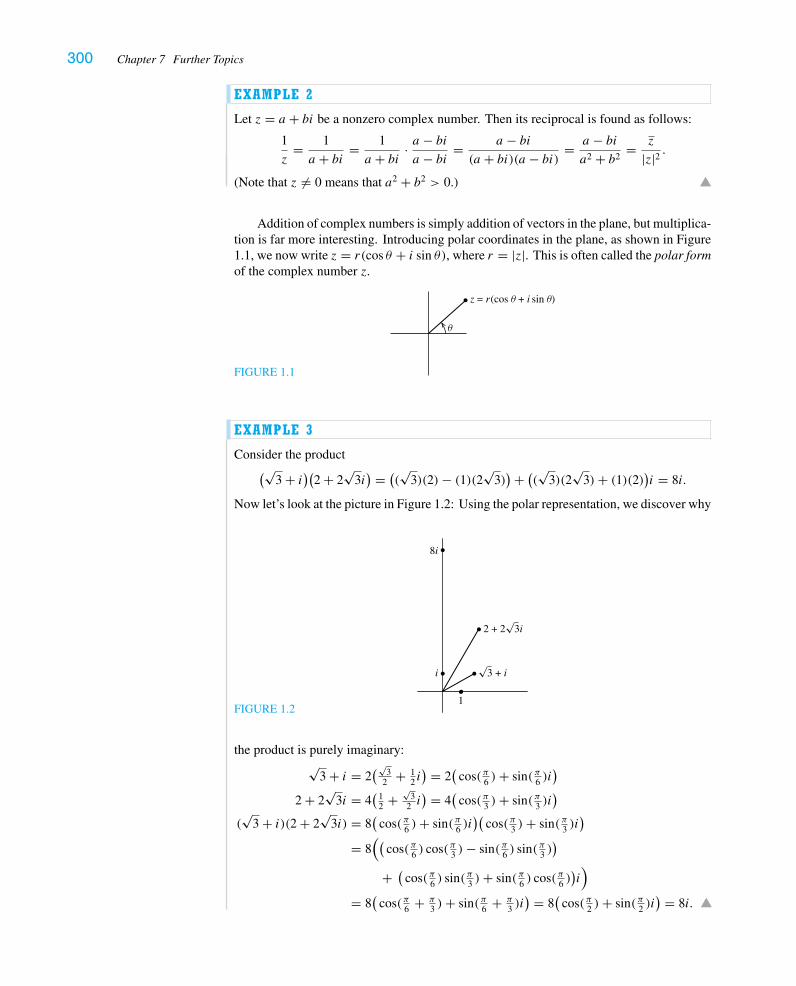
300 Chapter 7 Further Topics
EXAMPLE 2
Let z = a + bi be a nonzero complex number. Then its reciprocal is found as follows:
1
z= 1
a + bi = 1
a + bi · a − bia − bi = a − bi
(a + bi)(a − bi) = a − bia2 + b2
= z
|z|2 .
(Note that z �= 0 means that a2 + b2 > 0.)
Addition of complex numbers is simply addition of vectors in the plane, but multiplica-tion is far more interesting. Introducing polar coordinates in the plane, as shown in Figure1.1, we now write z = r(cos θ + i sin θ), where r = |z|. This is often called the polar formof the complex number z.
FIGURE 1.1
θ
z = r(cos θ + i sin θ)
EXAMPLE 3
Consider the product(√
3 + i)(2 + 2√
3i) = ((√3)(2)− (1)(2√
3))+ ((√3)(2
√3)+ (1)(2))i = 8i.
Now let’s look at the picture in Figure 1.2: Using the polar representation, we discover why
FIGURE 1.2
8i
1
i
2 + 2�3i
�3 + i
the product is purely imaginary:√
3 + i = 2(√
32 + 1
2 i) = 2
(cos( π6 )+ sin( π6 )i
)
2 + 2√
3i = 4(
12 +
√3
2 i) = 4
(cos( π3 )+ sin( π3 )i
)
(√
3 + i)(2 + 2√
3i) = 8(
cos( π6 )+ sin( π6 )i)(
cos( π3 )+ sin( π3 )i)
= 8((
cos( π6 ) cos( π3 )− sin( π6 ) sin( π3 ))
+ ( cos( π6 ) sin( π3 )+ sin( π6 ) cos( π6 ))i)
= 8(
cos( π6 + π3 )+ sin( π6 + π
3 )i) = 8
(cos( π2 )+ sin( π2 )i
) = 8i.
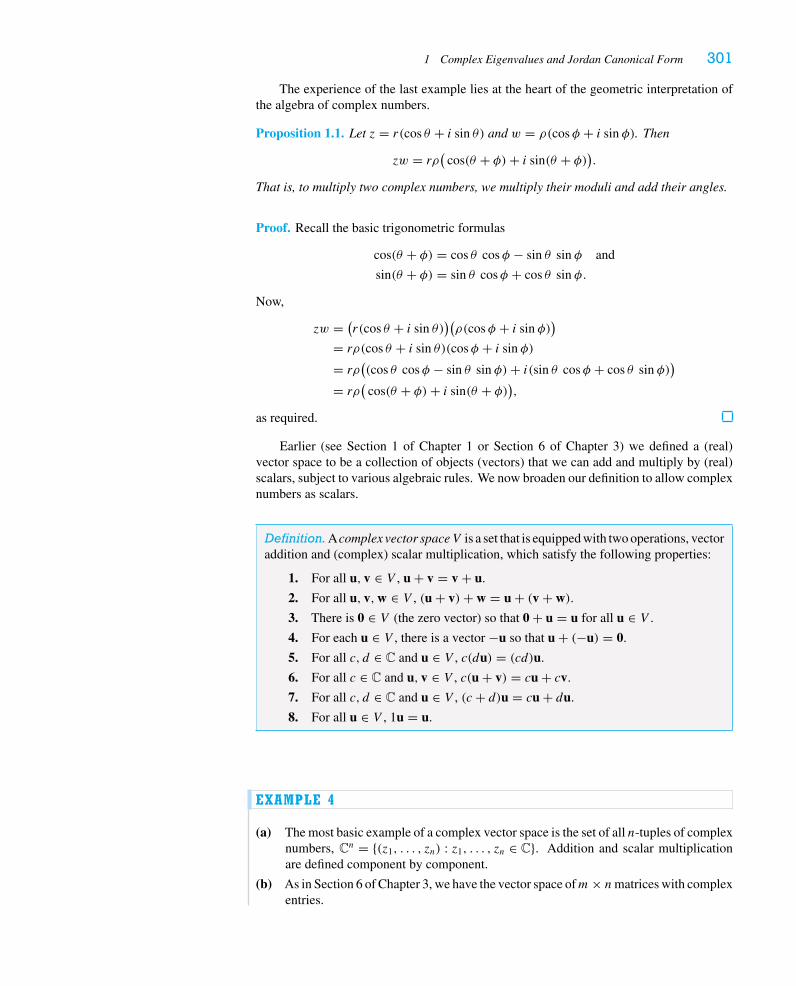
1 Complex Eigenvalues and Jordan Canonical Form 301
The experience of the last example lies at the heart of the geometric interpretation ofthe algebra of complex numbers.
Proposition 1.1. Let z = r(cos θ + i sin θ) and w = ρ(cosφ + i sin φ). Then
zw = rρ(
cos(θ + φ)+ i sin(θ + φ)).That is, to multiply two complex numbers, we multiply their moduli and add their angles.
Proof. Recall the basic trigonometric formulas
cos(θ + φ) = cos θ cosφ − sin θ sin φ and
sin(θ + φ) = sin θ cosφ + cos θ sin φ.
Now,
zw = (r(cos θ + i sin θ))(ρ(cosφ + i sin φ)
)
= rρ(cos θ + i sin θ)(cosφ + i sin φ)
= rρ((cos θ cosφ − sin θ sin φ)+ i(sin θ cosφ + cos θ sin φ)
)
= rρ(
cos(θ + φ)+ i sin(θ + φ)),as required.
Earlier (see Section 1 of Chapter 1 or Section 6 of Chapter 3) we defined a (real)vector space to be a collection of objects (vectors) that we can add and multiply by (real)scalars, subject to various algebraic rules. We now broaden our definition to allow complexnumbers as scalars.
Definition.Acomplex vector spaceV is a set that is equipped with two operations, vectoraddition and (complex) scalar multiplication, which satisfy the following properties:
1. For all u, v ∈ V , u + v = v + u.
2. For all u, v,w ∈ V , (u + v)+ w = u + (v + w).
3. There is 0 ∈ V (the zero vector) so that 0 + u = u for all u ∈ V .
4. For each u ∈ V , there is a vector −u so that u + (−u) = 0.
5. For all c, d ∈ C and u ∈ V , c(du) = (cd)u.
6. For all c ∈ C and u, v ∈ V , c(u + v) = cu + cv.
7. For all c, d ∈ C and u ∈ V , (c + d)u = cu + du.
8. For all u ∈ V , 1u = u.
EXAMPLE 4
(a) The most basic example of a complex vector space is the set of all n-tuples of complexnumbers, Cn = {(z1, . . . , zn) : z1, . . . , zn ∈ C}. Addition and scalar multiplicationare defined component by component.
(b) As in Section 6 of Chapter 3, we have the vector space ofm× nmatrices with complexentries.
302 Chapter 7 Further Topics
(c) Likewise, we have the vector space of complex-valued continuous functions on theinterval I. This vector space plays an important role in differential equations and inthe physics and mathematics of waves.
For us, the chief concern here is eigenvalues and eigenvectors. Now that we’ve ex-panded our world of scalars to the complex numbers, it is perfectly legitimate for a complexscalar λ to be an eigenvalue and for a nonzero vector v ∈ Cn to be an eigenvector of ann× n (perhaps real) matrix.
EXAMPLE 5
Consider the matrix
A =[
2 −5
1 0
].
We see that the characteristic polynomial of A is p(t) = t2 − 2t + 5, and so, applying thequadratic formula, the eigenvalues are 2±√
4−202 = 1 ± 2i. To find the eigenvectors, we
follow the usual procedure.
E(1 + 2i): We consider
A− (1 + 2i)I =[
1 − 2i −5
1 −1 − 2i
]
and read off the vector v1 = (1 + 2i, 1) as a basis vector.
E(1 − 2i): Now we consider
A− (1 − 2i)I =[
1 + 2i −5
1 −1 + 2i
],
and the vector v2 = (1 − 2i, 1) gives us a basis.
Note that v2 = v1; this should be no surprise, sinceAv1 = Av1 = (1 + 2i)v1 = (1 − 2i)v1.So, thinking of our matrix as representing a linear map from C2 to C2, we see that it can bediagonalized: With respect to the basis {v1, v2}, the matrix representing μA is the diagonalmatrix [
1 + 2i
1 − 2i
].
We can glean a bit more information about the underlying linear map μA from R2 toR2. Let
u1 =[
1
1
]and u2 =
[−2
0
].
Then v1 = u1 − iu2, and we interpret the eigenvector equation in terms of its real andimaginary parts:
A(u1 − iu2) = Av1 = (1 + 2i)v1 = (1 + 2i)(u1 − iu2) = (u1 + 2u2)+ i(2u1 − u2)
and so
Au1 = u1 + 2u2 and Au2 = −2u1 + u2.
1 Complex Eigenvalues and Jordan Canonical Form 303
That is, the matrix representing the linear map μA : R2 → R2 with respect to the basis{u1, u2} is [
1 −2
2 1
].
EXAMPLE 6
Let’s return to the matrix
A =
⎡⎢⎢⎢⎣
16
13 +
√6
616 −
√6
3
13 −
√6
623
13 +
√6
6
16 +
√6
313 −
√6
616
⎤⎥⎥⎥⎦ ,
which we first encountered in Exercise 4.3.24. A “short computation”1 reveals that thecharacteristic polynomial of this matrix is p(t) = −t3 + t2 − t + 1 = −(t − 1)(t2 + 1).Thus, A has one real eigenvalue, λ = 1, and two complex eigenvalues, ±i. We find thecomplex eigenvectors by considering the linear transformation μA : C3 → C3.
E(i): We find that v1 =⎡⎢⎣
1 − 2√
6i
2 + √6i
−5
⎤⎥⎦ gives a basis for
N(A− iI ) = N
⎛⎜⎜⎜⎝
⎡⎢⎢⎢⎣
16 − i 1
3 +√
66
16 −
√6
3
13 −
√6
623 − i 1
3 +√
66
16 +
√6
313 −
√6
616 − i
⎤⎥⎥⎥⎦
⎞⎟⎟⎟⎠ .
E(−i): Here v2 = v1 =⎡⎢⎣
1 + 2√
6i
2 − √6i
−5
⎤⎥⎦ gives a basis for N(A+ iI ). We can either calculate
this from scratch or reason that (A+ iI )v1 = (A− iI )v1 = 0, since A is a matrixwith real entries.
E(1): We see that v3 =⎡⎢⎣
1
2
1
⎤⎥⎦ gives a basis for
N(A− I ) = N
⎛⎜⎜⎜⎝
⎡⎢⎢⎢⎣
− 56
13 +
√6
616 −
√6
3
13 −
√6
6 − 13
13 +
√6
6
16 +
√6
313 −
√6
6 − 56
⎤⎥⎥⎥⎦
⎞⎟⎟⎟⎠ .
We should expect, following the reasoning of Section 2 of Chapter 6, that sinceA has threedistinct complex eigenvalues, we can diagonalize the matrix A working over C. Indeed,
1Although it is amusing to do the computations in this example by hand, this might be a reasonable place to givein and use a computer program such as Maple, Mathematica, or MATLAB.
304 Chapter 7 Further Topics
we leave it to the reader to check that, taking
P =
⎡⎢⎢⎣
1 − 2√
6i 1 + 2√
6i 1
2 + √6i 2 − √
6i 2
−5 −5 1
⎤⎥⎥⎦ and � =
⎡⎢⎢⎣i
−i1
⎤⎥⎥⎦ ,
we have A = P�P−1.But does this give us any insight into μA as a linear transformation from R3 to R3?
Letting
u1 =
⎡⎢⎢⎣
1
2
−5
⎤⎥⎥⎦ and u2 =
⎡⎢⎢⎣
2√
6
−√6
0
⎤⎥⎥⎦ ,
we see that v1 = u1 − iu2 and v2 = u1 + iu2. Since Av1 = iv1, it now follows that
A(u1 − iu2) = i(u1 − iu2) = u2 + iu1,
and so, using the fact that u1, u2, Au1, and Au2 are all real vectors, it must be the case that
Au1 = u2 and Au2 = −u1.
Furthermore, we notice that the vectors u1, u2, and v3 give an orthogonal basis for R3.SinceAv3 = v3 and the vectors u1 and u2 have the same length, we now infer thatμA givesa rotation of π/2 about the axis spanned by v3, fixing v3 and rotating u1 to u2 and u2 to−u1.
Theorem 2.1 of Chapter 6 is still valid when our scalars are complex numbers, and soCorollary 2.2 of Chapter 6 can be rephrased in our new setting:
Proposition 1.2. Suppose V is an n-dimensional complex vector space and T : V → V
has n distinct eigenvalues. Then T is diagonalizable.
It is important to remember that this result holds in the province of complex vectorspaces, with complex eigenvalues and complex eigenvectors. However, when we startwith a linear transformation on a real vector space, it is not too hard to extend the reasoningin Example 6 to deduce the following result.
Corollary 1.3. Suppose A is an n× n real matrix with n distinct (possibly complex)eigenvalues. Then A is similar to a “block diagonal” matrix of the form
⎡⎢⎢⎢⎢⎢⎢⎢⎢⎢⎢⎢⎢⎢⎢⎢⎢⎣
α1 −β1
β1 α1
. . .
αk −βkβk αk
λ2k+1
. . .
λn
⎤⎥⎥⎥⎥⎥⎥⎥⎥⎥⎥⎥⎥⎥⎥⎥⎥⎦
,
where α1 ± β1i, . . . , αk ± βki are the 2k complex eigenvalues (with βj �= 0) andλ2k+1, . . . , λn are the real eigenvalues.
1 Complex Eigenvalues and Jordan Canonical Form 305
Proof. Left to the reader in Exercise 3.
EXAMPLE 7
We wish to find the “block diagonal” form of the matrix
A =
⎡⎢⎢⎣
5 0 −2
8 7 −12
6 4 −7
⎤⎥⎥⎦
as guaranteed us by Corollary 1.3. The characteristic polynomial of A is p(t) = −t3 +5t2 − 11t + 15. Checking for rational roots, we find that λ = 3 is a real eigenvalue, and sowe find that p(t) = −(t − 3)(t2 − 2t + 5); thus, λ = 1 ± 2i are the complex eigenvaluesof A. The eigenvectors corresponding to the eigenvalues λ1 = 1 + 2i, λ2 = 1 − 2i, andλ3 = 3, respectively, are
v1 =
⎡⎢⎢⎣
2 + i7 + i
5
⎤⎥⎥⎦ , v2 =
⎡⎢⎢⎣
2 − i7 − i
5
⎤⎥⎥⎦ , and v3 =
⎡⎢⎢⎣
1
1
1
⎤⎥⎥⎦ .
Now, taking
u1 =
⎡⎢⎢⎣
2
7
5
⎤⎥⎥⎦ , u2 =
⎡⎢⎢⎣
−1
−1
0
⎤⎥⎥⎦ , and u3 = v3 =
⎡⎢⎢⎣
1
1
1
⎤⎥⎥⎦ ,
we see thatAv1 = A(u1 − iu2) = (1 + 2i)(u1 − iu2) = (u1 + 2u2)+ i(2u1 − u2), and so
Au1 = u1 + 2u2,
Au2 = −2u1 + u2,
Au3 = 3u3.
Thus, with respect to the basis B = {u1, u2, u3}, the linear transformation μA : R3 → R3
has the matrix ⎡⎢⎢⎣
1 −2 0
2 1 0
0 0 3
⎤⎥⎥⎦ .
Of course, since B is not an orthogonal basis (as we had in Example 6), the geometricinterpretation of μA is a bit more subtle: The line spanned by u3 is stretched by a factor of3, and the plane spanned by u1 and u2 is preserved.
Now we come to the much more subtle issue of what to do when the geometric multi-plicity of one eigenvalue (or more) is less than its algebraic multiplicity. To motivate thegeneral arguments, we consider the following example.
306 Chapter 7 Further Topics
EXAMPLE 8
Let
A =[
0 1
−4 4
].
Then the characteristic polynomial of A is p(t) = t2 − 4t + 4 = (t − 2)2. However, since
A− 2I =[−2 1
−4 2
],
we know that E(2) is only one-dimensional, with basis
v1 =[
1
2
],
and soA is not diagonalizable. However, we are fortunate enough to observe that the vectorv1 is obviously in the column space of the matrix A− 2I . Therefore, the equation
[−2 1
−4 2
]x =[
1
2
]
has a solution, for example:
v2 =[
0
1
].
Since (A− 2I )v2 = v1, we have Av2 = v1 + 2v2, and the matrix representing μA withrespect to the basis {v1, v2} is
J =[
2 1
0 2
].
This is called the Jordan canonical form of A.This argument applies generally to any 2 × 2 matrix A having eigenvalue λ with alge-
braic multiplicity 2 and geometric multiplicity 1. Let’s show that in this case we must haveN(A− λI) = C(A− λI). Assume not; then we choose a basis {v1} for N(A− λI) and abasis {v2} for C(A− λI); since v1 and v2 are nonparallel, we obtain a basis B = {v1, v2}for R2. What’s more, we can write v2 = (A− λI)x for some x ∈ R2, and so
Av2 = A(A− λI)x = (A− λI)(Ax)
is an element of C(A− λI). Since {v2} is a basis for this subspace, we infer thatAv2 = cv2
for some scalar c. Thus, the matrix representing μA with respect to the basis B is
B =[λ 0
0 c
],
contradicting the fact that A is not diagonalizable. Thus, we conclude that C(A− λI) =N(A− λI) and proceed as above to conclude that the Jordan canonical form of A is
[λ 1
0 λ
].
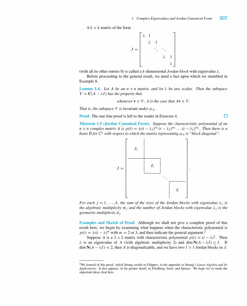
1 Complex Eigenvalues and Jordan Canonical Form 307
A k × k matrix of the form
J =
⎡⎢⎢⎢⎢⎢⎢⎢⎢⎣
λ 1
λ 1. . .
. . .
λ 1
λ
⎤⎥⎥⎥⎥⎥⎥⎥⎥⎦
(with all its other entries 0) is called a k-dimensional Jordan block with eigenvalue λ.Before proceeding to the general result, we need a fact upon which we stumbled in
Example 8.
Lemma 1.4. Let A be an n× n matrix, and let λ be any scalar. Then the subspaceV = C(A− λI) has the property that
whenever v ∈ V, it is the case that Av ∈ V.That is, the subspace V is invariant under μA.
Proof. The one-line proof is left to the reader in Exercise 4.
Theorem 1.5 (Jordan Canonical Form). Suppose the characteristic polynomial of ann× n complex matrix A is p(t) = ±(t − λ1)
m1(t − λ2)m2 . . . (t − λk)mk . Then there is a
basis B for Cn with respect to which the matrix representing μA is “block diagonal”:
J =
⎡⎢⎢⎢⎢⎢⎢⎢⎢⎢⎢⎢⎢⎢⎢⎢⎢⎢⎢⎣
J1
J2
. . .
Js
⎤⎥⎥⎥⎥⎥⎥⎥⎥⎥⎥⎥⎥⎥⎥⎥⎥⎥⎥⎦
.
For each j = 1, . . . , k, the sum of the sizes of the Jordan blocks with eigenvalue λj isthe algebraic multiplicity mj and the number of Jordan blocks with eigenvalue λj is thegeometric multiplicity dj .
Examples and Sketch of Proof. Although we shall not give a complete proof of thisresult here, we begin by examining what happens when the characteristic polynomial isp(t) = ±(t − λ)m with m = 2 or 3, and then indicate the general argument.2
Suppose A is a 2 × 2 matrix with characteristic polynomial p(t) = (t − λ)2. Thenλ is an eigenvalue of A (with algebraic multiplicity 2) and dim N(A− λI) ≥ 1. Ifdim N(A− λI) = 2, then A is diagonalizable, and we have two 1 × 1 Jordan blocks in J .
2We learned of this proof, which Strang credits to Filippov, in the appendix to Strang’s Linear Algebra and ItsApplications. It also appears, in far greater detail, in Friedberg, Insel, and Spence. We hope we’ve made theimportant ideas clear here.
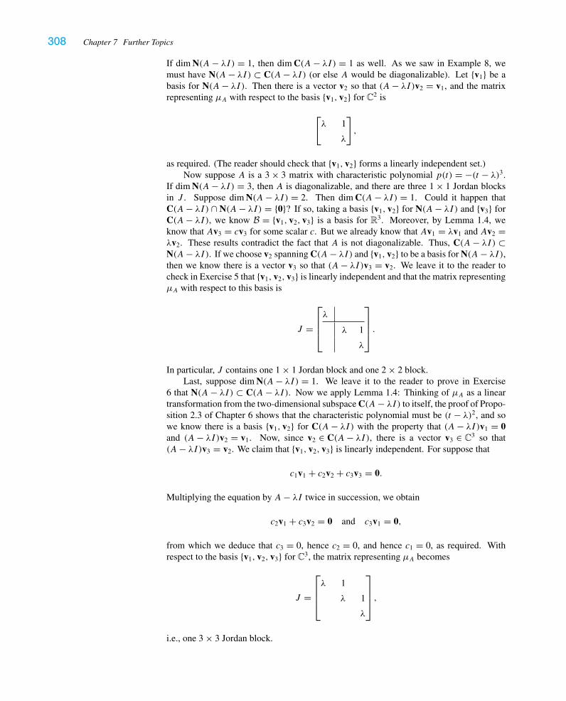
308 Chapter 7 Further Topics
If dim N(A− λI) = 1, then dim C(A− λI) = 1 as well. As we saw in Example 8, wemust have N(A− λI) ⊂ C(A− λI) (or else A would be diagonalizable). Let {v1} be abasis for N(A− λI). Then there is a vector v2 so that (A− λI)v2 = v1, and the matrixrepresenting μA with respect to the basis {v1, v2} for C2 is
[λ 1
λ
],
as required. (The reader should check that {v1, v2} forms a linearly independent set.)Now suppose A is a 3 × 3 matrix with characteristic polynomial p(t) = −(t − λ)3.
If dim N(A− λI) = 3, then A is diagonalizable, and there are three 1 × 1 Jordan blocksin J . Suppose dim N(A− λI) = 2. Then dim C(A− λI) = 1. Could it happen thatC(A− λI) ∩ N(A− λI) = {0}? If so, taking a basis {v1, v2} for N(A− λI) and {v3} forC(A− λI), we know B = {v1, v2, v3} is a basis for R3. Moreover, by Lemma 1.4, weknow that Av3 = cv3 for some scalar c. But we already know that Av1 = λv1 and Av2 =λv2. These results contradict the fact that A is not diagonalizable. Thus, C(A− λI) ⊂N(A− λI). If we choose v2 spanning C(A− λI) and {v1, v2} to be a basis for N(A− λI),then we know there is a vector v3 so that (A− λI)v3 = v2. We leave it to the reader tocheck in Exercise 5 that {v1, v2, v3} is linearly independent and that the matrix representingμA with respect to this basis is
J =
⎡⎢⎢⎣λ
λ 1
λ
⎤⎥⎥⎦ .
In particular, J contains one 1 × 1 Jordan block and one 2 × 2 block.Last, suppose dim N(A− λI) = 1. We leave it to the reader to prove in Exercise
6 that N(A− λI) ⊂ C(A− λI). Now we apply Lemma 1.4: Thinking of μA as a lineartransformation from the two-dimensional subspace C(A− λI) to itself, the proof of Propo-sition 2.3 of Chapter 6 shows that the characteristic polynomial must be (t − λ)2, and sowe know there is a basis {v1, v2} for C(A− λI) with the property that (A− λI)v1 = 0and (A− λI)v2 = v1. Now, since v2 ∈ C(A− λI), there is a vector v3 ∈ C3 so that(A− λI)v3 = v2. We claim that {v1, v2, v3} is linearly independent. For suppose that
c1v1 + c2v2 + c3v3 = 0.
Multiplying the equation by A− λI twice in succession, we obtain
c2v1 + c3v2 = 0 and c3v1 = 0,
from which we deduce that c3 = 0, hence c2 = 0, and hence c1 = 0, as required. Withrespect to the basis {v1, v2, v3} for C3, the matrix representing μA becomes
J =
⎡⎢⎢⎣λ 1
λ 1
λ
⎤⎥⎥⎦ ,
i.e., one 3 × 3 Jordan block.
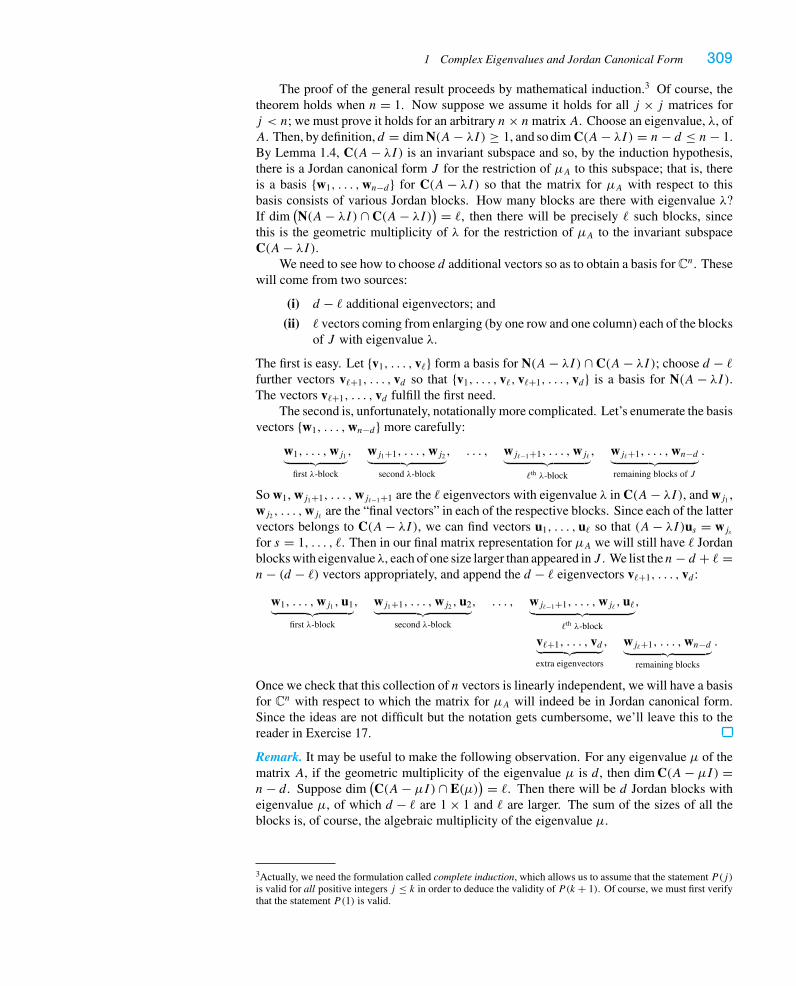
1 Complex Eigenvalues and Jordan Canonical Form 309
The proof of the general result proceeds by mathematical induction.3 Of course, thetheorem holds when n = 1. Now suppose we assume it holds for all j × j matrices forj < n; we must prove it holds for an arbitrary n× nmatrixA. Choose an eigenvalue, λ, ofA. Then, by definition, d = dim N(A− λI) ≥ 1, and so dim C(A− λI) = n− d ≤ n− 1.By Lemma 1.4, C(A− λI) is an invariant subspace and so, by the induction hypothesis,there is a Jordan canonical form J for the restriction of μA to this subspace; that is, thereis a basis {w1, . . . ,wn−d} for C(A− λI) so that the matrix for μA with respect to thisbasis consists of various Jordan blocks. How many blocks are there with eigenvalue λ?If dim
(N(A− λI) ∩ C(A− λI)) = , then there will be precisely such blocks, since
this is the geometric multiplicity of λ for the restriction of μA to the invariant subspaceC(A− λI).
We need to see how to choose d additional vectors so as to obtain a basis for Cn. Thesewill come from two sources:
(i) d − additional eigenvectors; and
(ii) vectors coming from enlarging (by one row and one column) each of the blocksof J with eigenvalue λ.
The first is easy. Let {v1, . . . , v} form a basis for N(A− λI) ∩ C(A− λI); choose d − further vectors v+1, . . . , vd so that {v1, . . . , v, v+1, . . . , vd} is a basis for N(A− λI).The vectors v+1, . . . , vd fulfill the first need.
The second is, unfortunately, notationally more complicated. Let’s enumerate the basisvectors {w1, . . . ,wn−d} more carefully:
w1, . . . ,wj1︸ ︷︷ ︸first λ-block
, wj1+1, . . . ,wj2︸ ︷︷ ︸second λ-block
, . . . , wj−1+1, . . . ,wj︸ ︷︷ ︸th λ-block
, wj+1, . . . ,wn−d︸ ︷︷ ︸remaining blocks of J
.
So w1, wj1+1, . . . ,wj−1+1 are the eigenvectors with eigenvalue λ in C(A− λI), and wj1 ,wj2 , . . . ,wj are the “final vectors” in each of the respective blocks. Since each of the lattervectors belongs to C(A− λI), we can find vectors u1, . . . ,u so that (A− λI)us = wjsfor s = 1, . . . , . Then in our final matrix representation for μA we will still have Jordanblocks with eigenvalueλ, each of one size larger than appeared inJ . We list then− d + =n− (d − ) vectors appropriately, and append the d − eigenvectors v+1, . . . , vd :
w1, . . . ,wj1 , u1︸ ︷︷ ︸first λ-block
, wj1+1, . . . ,wj2 , u2︸ ︷︷ ︸second λ-block
, . . . , wj−1+1, . . . ,wj , u︸ ︷︷ ︸th λ-block
,
v+1, . . . , vd︸ ︷︷ ︸extra eigenvectors
, wj+1, . . . ,wn−d︸ ︷︷ ︸remaining blocks
.
Once we check that this collection of n vectors is linearly independent, we will have a basisfor Cn with respect to which the matrix for μA will indeed be in Jordan canonical form.Since the ideas are not difficult but the notation gets cumbersome, we’ll leave this to thereader in Exercise 17.
Remark. It may be useful to make the following observation. For any eigenvalue μ of thematrix A, if the geometric multiplicity of the eigenvalue μ is d, then dim C(A− μI) =n− d . Suppose dim
(C(A− μI) ∩ E(μ)
) = . Then there will be d Jordan blocks witheigenvalue μ, of which d − are 1 × 1 and are larger. The sum of the sizes of all theblocks is, of course, the algebraic multiplicity of the eigenvalue μ.
3Actually, we need the formulation called complete induction, which allows us to assume that the statement P(j)is valid for all positive integers j ≤ k in order to deduce the validity of P(k + 1). Of course, we must first verifythat the statement P(1) is valid.
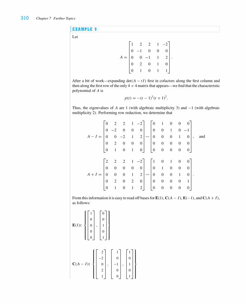
310 Chapter 7 Further Topics
EXAMPLE 9
Let
A =
⎡⎢⎢⎢⎢⎢⎢⎢⎣
1 2 2 1 −2
0 −1 0 0 0
0 0 −1 1 2
0 2 0 1 0
0 1 0 1 1
⎤⎥⎥⎥⎥⎥⎥⎥⎦.
After a bit of work—expanding det(A− tI ) first in cofactors along the first column andthen along the first row of the only 4 × 4 matrix that appears—we find that the characteristicpolynomial of A is
p(t) = −(t − 1)3(t + 1)2.
Thus, the eigenvalues of A are 1 (with algebraic multiplicity 3) and −1 (with algebraicmultiplicity 2). Performing row reduction, we determine that
A− I =
⎡⎢⎢⎢⎢⎢⎢⎢⎣
0 2 2 1 −2
0 −2 0 0 0
0 0 −2 1 2
0 2 0 0 0
0 1 0 1 0
⎤⎥⎥⎥⎥⎥⎥⎥⎦
�
⎡⎢⎢⎢⎢⎢⎢⎢⎣
0 1 0 0 0
0 0 1 0 −1
0 0 0 1 0
0 0 0 0 0
0 0 0 0 0
⎤⎥⎥⎥⎥⎥⎥⎥⎦, and
A+ I =
⎡⎢⎢⎢⎢⎢⎢⎢⎣
2 2 2 1 −2
0 0 0 0 0
0 0 0 1 2
0 2 0 2 0
0 1 0 1 2
⎤⎥⎥⎥⎥⎥⎥⎥⎦
�
⎡⎢⎢⎢⎢⎢⎢⎢⎣
1 0 1 0 0
0 1 0 0 0
0 0 0 1 0
0 0 0 0 1
0 0 0 0 0
⎤⎥⎥⎥⎥⎥⎥⎥⎦.
From this information it is easy to read off bases for E(1), C(A− I ), E(−1), and C(A+ I ),as follows:
E(1):
⎧⎪⎪⎪⎪⎪⎪⎨⎪⎪⎪⎪⎪⎪⎩
⎡⎢⎢⎢⎢⎢⎢⎣
1
0
0
0
0
⎤⎥⎥⎥⎥⎥⎥⎦,
⎡⎢⎢⎢⎢⎢⎢⎣
0
0
1
0
1
⎤⎥⎥⎥⎥⎥⎥⎦
⎫⎪⎪⎪⎪⎪⎪⎬⎪⎪⎪⎪⎪⎪⎭
C(A− I ):
⎧⎪⎪⎪⎪⎪⎪⎨⎪⎪⎪⎪⎪⎪⎩
⎡⎢⎢⎢⎢⎢⎢⎣
2
−2
0
2
1
⎤⎥⎥⎥⎥⎥⎥⎦,
⎡⎢⎢⎢⎢⎢⎢⎣
1
0
−1
0
0
⎤⎥⎥⎥⎥⎥⎥⎦,
⎡⎢⎢⎢⎢⎢⎢⎣
1
0
1
0
1
⎤⎥⎥⎥⎥⎥⎥⎦
⎫⎪⎪⎪⎪⎪⎪⎬⎪⎪⎪⎪⎪⎪⎭
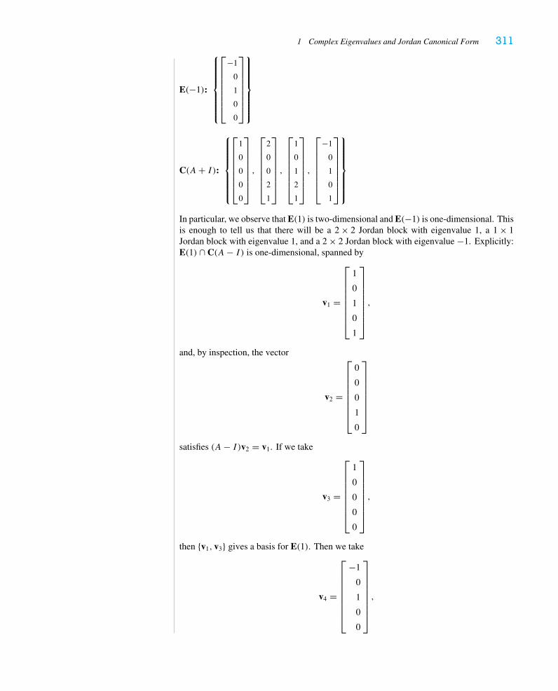
1 Complex Eigenvalues and Jordan Canonical Form 311
E(−1):
⎧⎪⎪⎪⎪⎪⎪⎨⎪⎪⎪⎪⎪⎪⎩
⎡⎢⎢⎢⎢⎢⎢⎣
−1
0
1
0
0
⎤⎥⎥⎥⎥⎥⎥⎦
⎫⎪⎪⎪⎪⎪⎪⎬⎪⎪⎪⎪⎪⎪⎭
C(A+ I ):
⎧⎪⎪⎪⎪⎪⎪⎨⎪⎪⎪⎪⎪⎪⎩
⎡⎢⎢⎢⎢⎢⎢⎣
1
0
0
0
0
⎤⎥⎥⎥⎥⎥⎥⎦,
⎡⎢⎢⎢⎢⎢⎢⎣
2
0
0
2
1
⎤⎥⎥⎥⎥⎥⎥⎦,
⎡⎢⎢⎢⎢⎢⎢⎣
1
0
1
2
1
⎤⎥⎥⎥⎥⎥⎥⎦,
⎡⎢⎢⎢⎢⎢⎢⎣
−1
0
1
0
1
⎤⎥⎥⎥⎥⎥⎥⎦
⎫⎪⎪⎪⎪⎪⎪⎬⎪⎪⎪⎪⎪⎪⎭
In particular, we observe that E(1) is two-dimensional and E(−1) is one-dimensional. Thisis enough to tell us that there will be a 2 × 2 Jordan block with eigenvalue 1, a 1 × 1Jordan block with eigenvalue 1, and a 2 × 2 Jordan block with eigenvalue −1. Explicitly:E(1) ∩ C(A− I ) is one-dimensional, spanned by
v1 =
⎡⎢⎢⎢⎢⎢⎢⎢⎣
1
0
1
0
1
⎤⎥⎥⎥⎥⎥⎥⎥⎦,
and, by inspection, the vector
v2 =
⎡⎢⎢⎢⎢⎢⎢⎢⎣
0
0
0
1
0
⎤⎥⎥⎥⎥⎥⎥⎥⎦
satisfies (A− I )v2 = v1. If we take
v3 =
⎡⎢⎢⎢⎢⎢⎢⎢⎣
1
0
0
0
0
⎤⎥⎥⎥⎥⎥⎥⎥⎦,
then {v1, v3} gives a basis for E(1). Then we take
v4 =
⎡⎢⎢⎢⎢⎢⎢⎢⎣
−1
0
1
0
0
⎤⎥⎥⎥⎥⎥⎥⎥⎦,

312 Chapter 7 Further Topics
which spans E(−1), and observe (as we saw in Example 8 and the proof of Theorem 1.5)that E(−1) ⊂ C(A+ I ), and so we find
v5 =
⎡⎢⎢⎢⎢⎢⎢⎢⎣
0
−1
0
1
0
⎤⎥⎥⎥⎥⎥⎥⎥⎦
with the property that (A+ I )v5 = v4. The theory tells us that {v1, v2, v3, v4, v5} must bea linearly independent set, hence a basis for C5, and with respect to this basis we obtain theJordan canonical form
J =
⎡⎢⎢⎢⎢⎢⎢⎢⎢⎣
1 1
0 1
1
−1 1
0 −1
⎤⎥⎥⎥⎥⎥⎥⎥⎥⎦.
Exercises 7.1
1. Suppose A is a real 2 × 2 matrix with complex eigenvalues α ± βi, and suppose v =x − iy is the eigenvector corresponding to α + βi. (Here x, y ∈ R2.)a. First, explain why the eigenvalues of A must be complex conjugates.
b. Show that the matrix for μA with respect to the basis {x, y} is[α −ββ α
].
2. Find the eigenvalues and eigenvectors of the following real matrices, and give baseswith respect to which the matrix is (i) diagonalized as a complex linear transformation;(ii) in the “block diagonal” form provided by Corollary 1.3.
a.
[2 1
−1 2
]
b.∗[
1 1
−2 3
]
c.∗
⎡⎢⎣
1 1 2
−1 1 0
0 0 2
⎤⎥⎦
d.
⎡⎢⎢⎢⎣
3 −1 3 −1
3 3 −1 −1
−1 −1 3 3
−1 3 −1 3
⎤⎥⎥⎥⎦
e.
⎡⎢⎢⎢⎣
3 −2 0 1
2 3 1 0
0 1 3 2
1 0 −2 3
⎤⎥⎥⎥⎦
3. Prove Corollary 1.3. (Hint: Generalize the argument in Exercise 1.)
4. Prove Lemma 1.4.
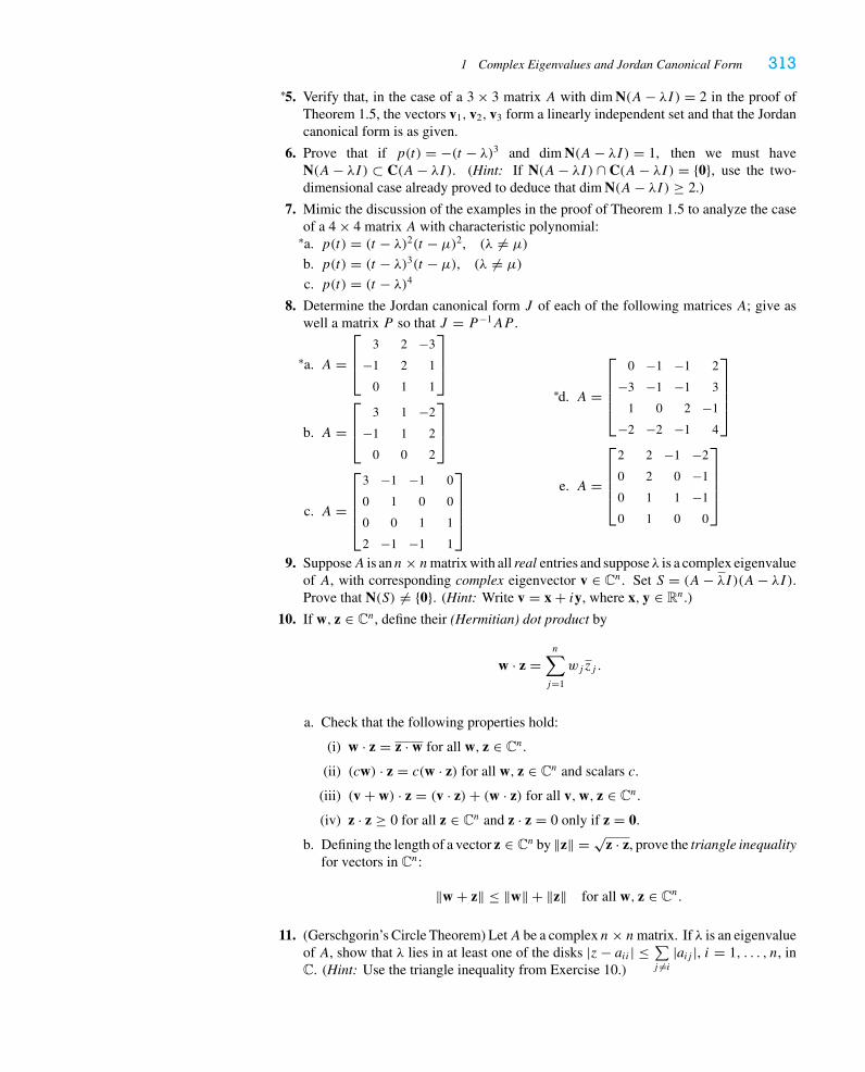
1 Complex Eigenvalues and Jordan Canonical Form 313
5.∗ Verify that, in the case of a 3 × 3 matrix A with dim N(A− λI) = 2 in the proof ofTheorem 1.5, the vectors v1, v2, v3 form a linearly independent set and that the Jordancanonical form is as given.
6. Prove that if p(t) = −(t − λ)3 and dim N(A− λI) = 1, then we must haveN(A− λI) ⊂ C(A− λI). (Hint: If N(A− λI) ∩ C(A− λI) = {0}, use the two-dimensional case already proved to deduce that dim N(A− λI) ≥ 2.)
7. Mimic the discussion of the examples in the proof of Theorem 1.5 to analyze the caseof a 4 × 4 matrix A with characteristic polynomial:a.∗ p(t) = (t − λ)2(t − μ)2, (λ �= μ)
b. p(t) = (t − λ)3(t − μ), (λ �= μ)
c. p(t) = (t − λ)48. Determine the Jordan canonical form J of each of the following matrices A; give as
well a matrix P so that J = P−1AP .
a.∗ A =⎡⎢⎣
3 2 −3
−1 2 1
0 1 1
⎤⎥⎦
b. A =⎡⎢⎣
3 1 −2
−1 1 2
0 0 2
⎤⎥⎦
c. A =
⎡⎢⎢⎢⎣
3 −1 −1 0
0 1 0 0
0 0 1 1
2 −1 −1 1
⎤⎥⎥⎥⎦
d.∗ A =
⎡⎢⎢⎢⎣
0 −1 −1 2
−3 −1 −1 3
1 0 2 −1
−2 −2 −1 4
⎤⎥⎥⎥⎦
e. A =
⎡⎢⎢⎢⎣
2 2 −1 −2
0 2 0 −1
0 1 1 −1
0 1 0 0
⎤⎥⎥⎥⎦
9. SupposeA is ann× nmatrix with all real entries and supposeλ is a complex eigenvalueof A, with corresponding complex eigenvector v ∈ Cn. Set S = (A− λI)(A− λI).Prove that N(S) �= {0}. (Hint: Write v = x + iy, where x, y ∈ Rn.)
10. If w, z ∈ Cn, define their (Hermitian) dot product by
w · z =n∑j=1
wjzj .
a. Check that the following properties hold:
(i) w · z = z · w for all w, z ∈ Cn.
(ii) (cw) · z = c(w · z) for all w, z ∈ Cn and scalars c.
(iii) (v + w) · z = (v · z)+ (w · z) for all v,w, z ∈ Cn.
(iv) z · z ≥ 0 for all z ∈ Cn and z · z = 0 only if z = 0.
b. Defining the length of a vector z ∈ Cn by ‖z‖ = √z · z, prove the triangle inequality
for vectors in Cn:
‖w + z‖ ≤ ‖w‖ + ‖z‖ for all w, z ∈ Cn.
11. (Gerschgorin’s Circle Theorem) LetA be a complex n× nmatrix. If λ is an eigenvalueof A, show that λ lies in at least one of the disks |z− aii | ≤ ∑
j �=i|aij |, i = 1, . . . , n, in
C. (Hint: Use the triangle inequality from Exercise 10.)
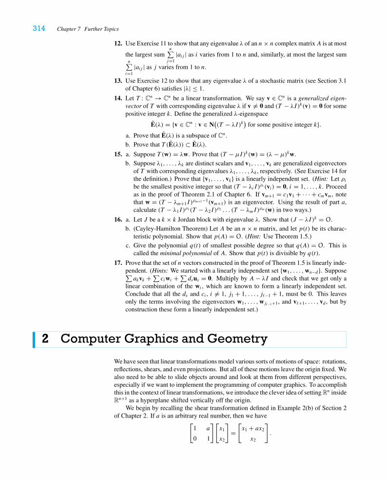
314 Chapter 7 Further Topics
12. Use Exercise 11 to show that any eigenvalue λ of an n× n complex matrixA is at most
the largest sumn∑j=1
|aij | as i varies from 1 to n and, similarly, at most the largest sumn∑i=1
|aij | as j varies from 1 to n.
13. Use Exercise 12 to show that any eigenvalue λ of a stochastic matrix (see Section 3.1of Chapter 6) satisfies |λ| ≤ 1.
14. Let T : Cn → Cn be a linear transformation. We say v ∈ Cn is a generalized eigen-vector of T with corresponding eigenvalue λ if v �= 0 and (T − λI)k(v) = 0 for somepositive integer k. Define the generalized λ-eigenspace
E(λ) = {v ∈ Cn : v ∈ N((T − λI)k) for some positive integer k}.
a. Prove that E(λ) is a subspace of Cn.
b. Prove that T (E(λ)) ⊂ E(λ).
15. a. Suppose T (w) = λw. Prove that (T − μI)k(w) = (λ− μ)kw.
b. Suppose λ1, . . . , λk are distinct scalars and v1, . . . , vk are generalized eigenvectorsof T with corresponding eigenvalues λ1, . . . , λk , respectively. (See Exercise 14 forthe definition.) Prove that {v1, . . . , vk} is a linearly independent set. (Hint: Let ρibe the smallest positive integer so that (T − λiI )ρi (vi ) = 0, i = 1, . . . , k. Proceedas in the proof of Theorem 2.1 of Chapter 6. If vm+1 = c1v1 + · · · + cmvm, notethat w = (T − λm+1I )
ρm+1−1(vm+1) is an eigenvector. Using the result of part a,calculate (T − λ1I )
ρ1(T − λ2I )ρ2 . . . (T − λmI)ρm(w) in two ways.)
16. a. Let J be a k × k Jordan block with eigenvalue λ. Show that (J − λI)k = O.
b. (Cayley-Hamilton Theorem) Let A be an n× n matrix, and let p(t) be its charac-teristic polynomial. Show that p(A) = O. (Hint: Use Theorem 1.5.)
c. Give the polynomial q(t) of smallest possible degree so that q(A) = O. This iscalled the minimal polynomial of A. Show that p(t) is divisible by q(t).
17. Prove that the set of n vectors constructed in the proof of Theorem 1.5 is linearly inde-pendent. (Hints: We started with a linearly independent set {w1, . . . ,wn−d}. Suppose∑akvk +∑ ciwi +∑ dsus = 0. Multiply by A− λI and check that we get only a
linear combination of the wi , which are known to form a linearly independent set.Conclude that all the ds and ci , i �= 1, j1 + 1, . . . , j−1 + 1, must be 0. This leavesonly the terms involving the eigenvectors w1, . . . ,wj−1+1, and v+1, . . . , vd , but byconstruction these form a linearly independent set.)
2 Computer Graphics and Geometry
We have seen that linear transformations model various sorts of motions of space: rotations,reflections, shears, and even projections. But all of these motions leave the origin fixed. Wealso need to be able to slide objects around and look at them from different perspectives,especially if we want to implement the programming of computer graphics. To accomplishthis in the context of linear transformations, we introduce the clever idea of setting Rn insideRn+1 as a hyperplane shifted vertically off the origin.
We begin by recalling the shear transformation defined in Example 2(b) of Section 2of Chapter 2. If a is an arbitrary real number, then we have
[1 a
0 1
][x1
x2
]=[x1 + ax2
x2
].
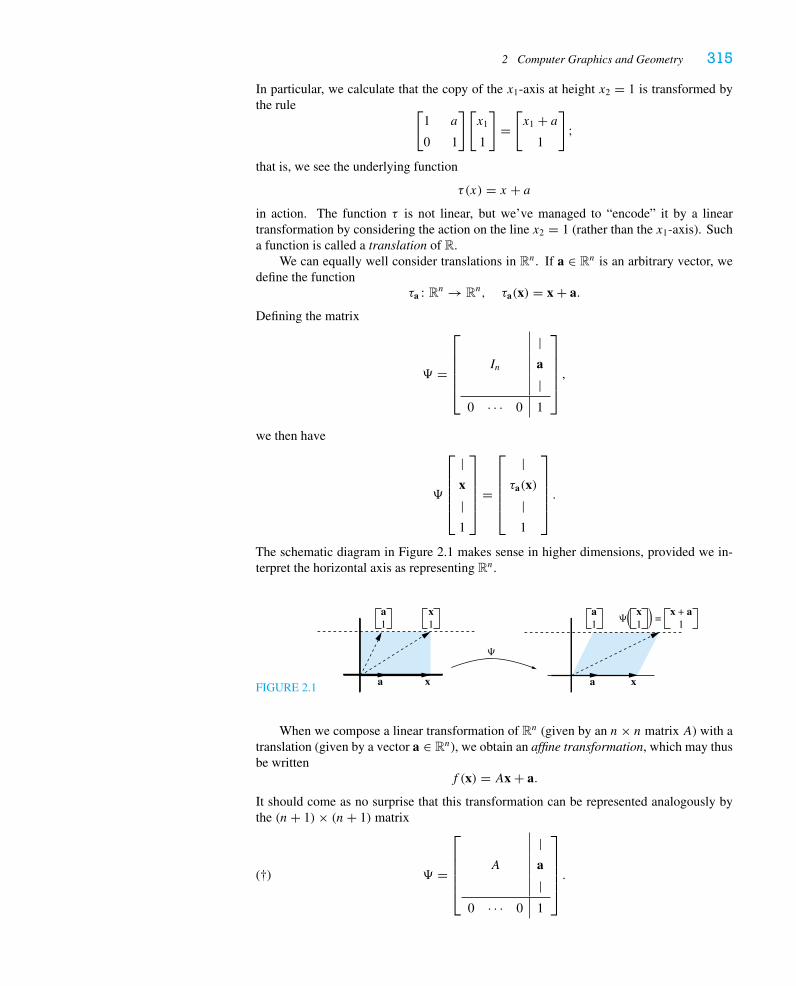
2 Computer Graphics and Geometry 315
In particular, we calculate that the copy of the x1-axis at height x2 = 1 is transformed bythe rule [
1 a
0 1
][x1
1
]=[x1 + a
1
];
that is, we see the underlying function
τ(x) = x + ain action. The function τ is not linear, but we’ve managed to “encode” it by a lineartransformation by considering the action on the line x2 = 1 (rather than the x1-axis). Sucha function is called a translation of R.
We can equally well consider translations in Rn. If a ∈ Rn is an arbitrary vector, wedefine the function
τa : Rn → Rn, τa(x) = x + a.
Defining the matrix
� =
⎡⎢⎢⎢⎢⎣
|In a
|0 · · · 0 1
⎤⎥⎥⎥⎥⎦,
we then have
�
⎡⎢⎢⎢⎢⎣
|x
|1
⎤⎥⎥⎥⎥⎦
=
⎡⎢⎢⎢⎢⎣
|τa(x)
|1
⎤⎥⎥⎥⎥⎦.
The schematic diagram in Figure 2.1 makes sense in higher dimensions, provided we in-terpret the horizontal axis as representing Rn.
FIGURE 2.1
�
a x
a1
a1
x1
x1
x + a1
a x
�( ) =
When we compose a linear transformation of Rn (given by an n× n matrix A) with atranslation (given by a vector a ∈ Rn), we obtain an affine transformation, which may thusbe written
f (x) = Ax + a.
It should come as no surprise that this transformation can be represented analogously bythe (n+ 1)× (n+ 1) matrix
(†) � =
⎡⎢⎢⎢⎢⎣
|A a
|0 · · · 0 1
⎤⎥⎥⎥⎥⎦.
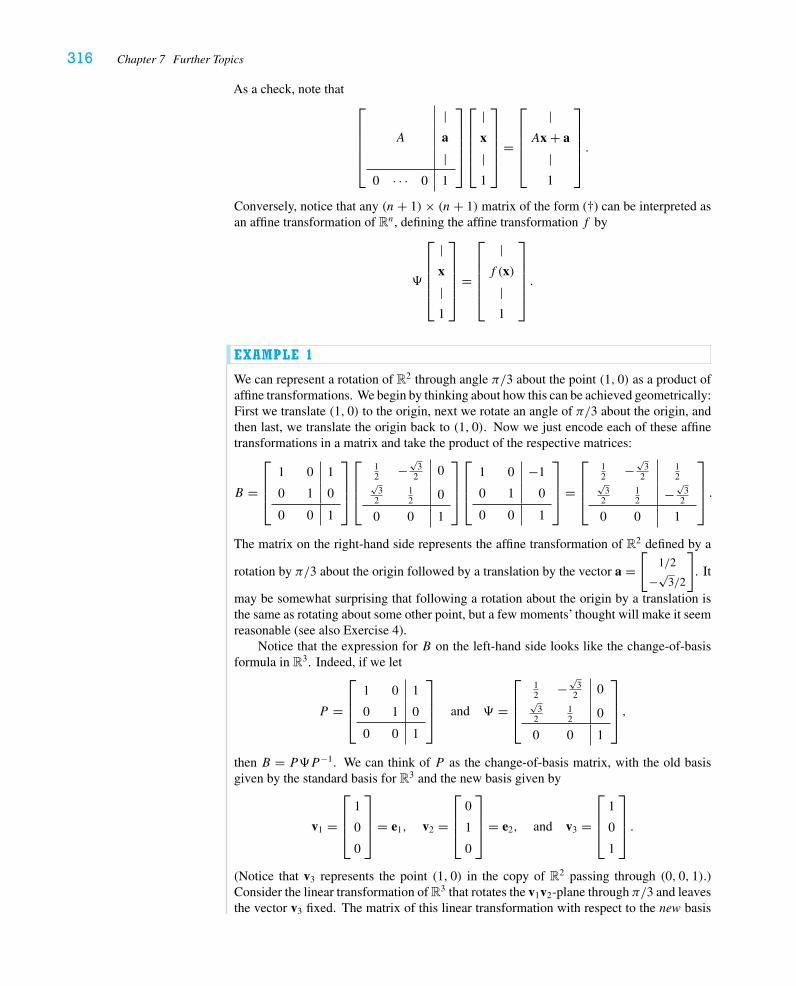
316 Chapter 7 Further Topics
As a check, note that⎡⎢⎢⎢⎢⎣
|A a
|0 · · · 0 1
⎤⎥⎥⎥⎥⎦
⎡⎢⎢⎢⎢⎣
|x
|1
⎤⎥⎥⎥⎥⎦
=
⎡⎢⎢⎢⎢⎣
|Ax + a
|1
⎤⎥⎥⎥⎥⎦.
Conversely, notice that any (n+ 1)× (n+ 1) matrix of the form (†) can be interpreted asan affine transformation of Rn, defining the affine transformation f by
�
⎡⎢⎢⎢⎢⎣
|x
|1
⎤⎥⎥⎥⎥⎦
=
⎡⎢⎢⎢⎢⎣
|f (x)
|1
⎤⎥⎥⎥⎥⎦.
EXAMPLE 1
We can represent a rotation of R2 through angle π/3 about the point (1, 0) as a product ofaffine transformations. We begin by thinking about how this can be achieved geometrically:First we translate (1, 0) to the origin, next we rotate an angle of π/3 about the origin, andthen last, we translate the origin back to (1, 0). Now we just encode each of these affinetransformations in a matrix and take the product of the respective matrices:
B =
⎡⎢⎢⎣
1 0 1
0 1 0
0 0 1
⎤⎥⎥⎦
⎡⎢⎢⎣
12 −
√3
2 0√
32
12 0
0 0 1
⎤⎥⎥⎦
⎡⎢⎢⎣
1 0 −1
0 1 0
0 0 1
⎤⎥⎥⎦ =
⎡⎢⎢⎣
12 −
√3
212√
32
12 −
√3
2
0 0 1
⎤⎥⎥⎦ .
The matrix on the right-hand side represents the affine transformation of R2 defined by a
rotation by π/3 about the origin followed by a translation by the vector a =[
1/2
−√3/2
]. It
may be somewhat surprising that following a rotation about the origin by a translation isthe same as rotating about some other point, but a few moments’ thought will make it seemreasonable (see also Exercise 4).
Notice that the expression for B on the left-hand side looks like the change-of-basisformula in R3. Indeed, if we let
P =
⎡⎢⎢⎣
1 0 1
0 1 0
0 0 1
⎤⎥⎥⎦ and � =
⎡⎢⎢⎣
12 −
√3
2 0√
32
12 0
0 0 1
⎤⎥⎥⎦ ,
then B = P�P−1. We can think of P as the change-of-basis matrix, with the old basisgiven by the standard basis for R3 and the new basis given by
v1 =
⎡⎢⎢⎣
1
0
0
⎤⎥⎥⎦ = e1, v2 =
⎡⎢⎢⎣
0
1
0
⎤⎥⎥⎦ = e2, and v3 =
⎡⎢⎢⎣
1
0
1
⎤⎥⎥⎦ .
(Notice that v3 represents the point (1, 0) in the copy of R2 passing through (0, 0, 1).)Consider the linear transformation of R3 that rotates the v1v2-plane through π/3 and leavesthe vector v3 fixed. The matrix of this linear transformation with respect to the new basis
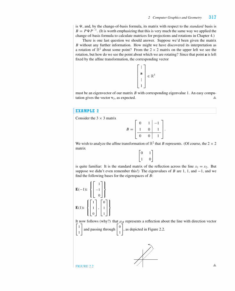
2 Computer Graphics and Geometry 317
is �, and, by the change-of-basis formula, its matrix with respect to the standard basis isB = P�P−1. (It is worth emphasizing that this is very much the same way we applied thechange-of-basis formula to calculate matrices for projections and rotations in Chapter 4.)
There is one last question we should answer. Suppose we’d been given the matrixB without any further information. How might we have discovered its interpretation asa rotation of R2 about some point? From the 2 × 2 matrix on the upper left we see therotation, but how do we see the point about which we are rotating? Since that point a is leftfixed by the affine transformation, the corresponding vector
⎡⎢⎢⎢⎢⎣
|a
|1
⎤⎥⎥⎥⎥⎦
∈ R3
must be an eigenvector of our matrix B with corresponding eigenvalue 1. An easy compu-tation gives the vector v3, as expected.
EXAMPLE 2
Consider the 3 × 3 matrix
B =
⎡⎢⎢⎣
0 1 −1
1 0 1
0 0 1
⎤⎥⎥⎦ .
We wish to analyze the affine transformation of R2 that B represents. (Of course, the 2 × 2matrix [
0 1
1 0
]
is quite familiar: It is the standard matrix of the reflection across the line x1 = x2. Butsuppose we didn’t even remember this!) The eigenvalues of B are 1, 1, and −1, and wefind the following bases for the eigenspaces of B:
E(−1):
⎧⎪⎨⎪⎩
⎡⎢⎣
1
−1
0
⎤⎥⎦
⎫⎪⎬⎪⎭
E(1):
⎧⎪⎨⎪⎩
⎡⎢⎣
1
1
0
⎤⎥⎦ ,
⎡⎢⎣
0
1
1
⎤⎥⎦
⎫⎪⎬⎪⎭
It now follows (why?) that μB represents a reflection about the line with direction vector[1
1
]and passing through
[0
1
], as depicted in Figure 2.2.
FIGURE 2.2
318 Chapter 7 Further Topics
EXAMPLE 3
Consider next the 3 × 3 matrix
B =
⎡⎢⎢⎣
12
√3
2 1√
32 − 1
2 0
0 0 1
⎤⎥⎥⎦ .
What do eigenvalues and eigenvectors tell us about B? The characteristic polynomialof B is p(t) = −(t − 1)2(t + 1), so the eigenvalue −1 has algebraic multiplicity 1 andthe eigenvalue 1 has algebraic multiplicity 2. We determine the following bases for theeigenspaces of B:
E(−1):
⎧⎪⎨⎪⎩
⎡⎢⎣
12
−√
32
0
⎤⎥⎦
⎫⎪⎬⎪⎭
E(1):
⎧⎪⎨⎪⎩
⎡⎢⎣
√3
212
0
⎤⎥⎦
⎫⎪⎬⎪⎭
Unfortunately, the geometric multiplicity of the eigenvalue 1 is only 1. But consider thevector
v =
⎡⎢⎢⎣
12
0
1
⎤⎥⎥⎦ ;
we have
B =
⎡⎢⎢⎣
12
√3
2 1√
32 − 1
2 0
0 0 1
⎤⎥⎥⎦
⎡⎢⎢⎣
12
0
1
⎤⎥⎥⎦ =
⎡⎢⎢⎣
54
√3
4
1
⎤⎥⎥⎦ =
⎡⎢⎢⎣
12
0
1
⎤⎥⎥⎦+
√3
2
⎡⎢⎢⎣
√3
2
12
0
⎤⎥⎥⎦ .
That is, Bv is equal to the sum of v and a scalar multiple of the (unit) vector spanning E(1).With respect to the basis formed by
v1 =
⎡⎢⎢⎣
12
−√
32
0
⎤⎥⎥⎦ , v2 =
⎡⎢⎢⎣
√3
2
12
0
⎤⎥⎥⎦ , and v3 =
⎡⎢⎢⎣
12
0
1
⎤⎥⎥⎦ ,
the matrix representing μB is
� =
⎡⎢⎢⎣
−1 0 0
0 1√
32
0 0 1
⎤⎥⎥⎦ .
From this we infer that μB gives a reflection of R2 about the line spanned by v2 and thentranslates by the vector
√3
2 v2. This is called a glide reflection with axis v2.
2 Computer Graphics and Geometry 319
2.1 Isometries of R and R2
Of particular interest are the isometries of Rn: these are the functions f : Rn → Rn thatpreserve distance, i.e.,
‖f (x)− f (y)‖ = ‖x − y‖ for all x, y ∈ Rn.
Lemma 2.1. Every isometry f : Rn → Rn can be written in the form
f (x) = Ax + a
for some vector a ∈ Rn and some orthogonal n× n matrix A.
Proof. Let T : Rn → Rn be defined by T (x) = f (x)− f (0). Then we observe that T (0) =f (0)− f (0) = 0, and T is also an isometry:
‖T (x)− T (y)‖ = ‖(f (x)− f (0))− (f (y)− f (0))‖ = ‖f (x)− f (y)‖ = ‖x − y‖,as desired. It now follows from Exercise 4.4.23 that T is a linear transformation whosestandard matrix is orthogonal.
Corollary 2.2. Every isometry of Rn is given by an (n+ 1)× (n+ 1) matrix of the form⎡⎢⎢⎢⎢⎣
|A a
|0 · · · 0 1
⎤⎥⎥⎥⎥⎦,
where a ∈ Rn and A is an orthogonal n× n matrix.
We can now use our experience with linear algebra to classify all isometries of R andR2. The analogous project for R3 is left for Exercise 13. Our first result is hardly a surprise,but it’s a good warm-up for what is to follow.
Proposition 2.3. Every isometry of R is either a translation or a reflection.
Proof. Since the only orthogonal 1 × 1 matrices are [1] and [−1], it is a matter of analyzingthe 2 × 2 matrices [
1 a
0 1
]and
[−1 a
0 1
].
We understand that the former represents a translation (by a) as it stands. What about thelatter? Since the matrix is upper triangular, we recognize that its eigenvalues are −1 and 1,the corresponding eigenvectors being[
1
0
]and
[a/2
1
].
This tells us that the isometry in question leaves the point a/2 fixed and reflects about it.Note that the change-of-basis formula gives[
−1 a
0 1
]=[
1 a2
0 1
][−1 0
0 1
][1 − a
2
0 1
].
Multiplying by
[x
1
]yields
[−1 a
0 1
][x
1
]=[
1 a2
0 1
][−(x − a
2 )
1
]=[−(x − a
2 )+ a2
1
],
as one can check easily by elementary algebra.
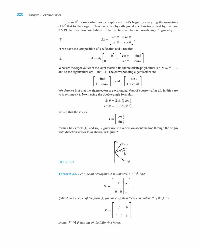
320 Chapter 7 Further Topics
Life in R2 is somewhat more complicated. Let’s begin by analyzing the isometriesof R2 that fix the origin. These are given by orthogonal 2 × 2 matrices, and by Exercise2.5.19, there are two possibilities: Either we have a rotation through angle θ , given by
(†) Aθ =[
cos θ − sin θ
sin θ cos θ
],
or we have the composition of a reflection and a rotation:
(‡) A = Aθ
[1 0
0 −1
]=[
cos θ sin θ
sin θ − cos θ
].
What are the eigenvalues of the latter matrix? Its characteristic polynomial isp(t) = t2 − 1,and so the eigenvalues are 1 and −1. The corresponding eigenvectors are
[sin θ
1 − cos θ
]and
[− sin θ
1 + cos θ
].
We observe first that the eigenvectors are orthogonal (but of course—after all, in this caseA is symmetric). Next, using the double-angle formulas
sin θ = 2 sin θ2 cos θ2
cos θ = 1 − 2 sin2 θ2 ,
we see that the vector
v =[
cos θ2sin θ
2
]
forms a basis for E(1), and so μA gives rise to a reflection about the line through the originwith direction vector v, as shown in Figure 2.3.
FIGURE 2.3
e2
v
e1
T(e2)
T(e1)
θ/2
Theorem 2.4. Let A be an orthogonal 2 × 2 matrix, a ∈ R2, and
� =
⎡⎢⎢⎣
A a
0 0 1
⎤⎥⎥⎦ .
If detA = 1 (i.e., is of the form (†) for some θ ), then there is a matrix P of the form
P =
⎡⎢⎢⎣
I b
0 0 1
⎤⎥⎥⎦
so that P−1�P has one of the following forms:
2 Computer Graphics and Geometry 321
1.
⎡⎢⎣
1 0 a1
0 1 a2
0 0 1
⎤⎥⎦ (a translation)
2.
⎡⎢⎣
cos θ − sin θ 0
sin θ cos θ 0
0 0 1
⎤⎥⎦ (a rotation) .
And if detA = −1 (i.e., is of the form (‡) for some θ ), then there is a matrix P of the form
P =
⎡⎢⎢⎣
B b
0 0 1
⎤⎥⎥⎦ ,
where B is a rotation matrix, so that P−1�P has the one of the following forms:
3.
⎡⎢⎣
−1 0 0
0 1 0
0 0 1
⎤⎥⎦ (a reflection)
4.
⎡⎢⎣
−1 0 0
0 1 a
0 0 1
⎤⎥⎦ (a glide reflection when a �= 0).
Moreover, case 3 occurs precisely when a = a1 cos θ2 + a2 sin θ2 = 0.
Proof. When A = I , we have case 1. Next we consider what happens when
A = Aθ =[
cos θ − sin θ
sin θ cos θ
].
Then 1 is an eigenvalue of the matrix � with algebraic multiplicity 1. A corresponding
eigenvector v3 must be a scalar multiple of the vector
⎡⎢⎢⎢⎣
|b
|1
⎤⎥⎥⎥⎦ for some b ∈ R2, since 1 is not
an eigenvalue of A. Thus, {e1, e2, v3} gives a basis for R3, and with respect to that basis,the matrix becomes that in case 2. (See Exercise 4.)
When A is an orthogonal matrix with detA = −1, then A is of the form
A =[
cos θ sin θ
sin θ − cos θ
]
for some θ . This case is somewhat more interesting, as this matrix has eigenvalues −1 and1, and hence the eigenvalues of � are −1, 1, and 1. When E(1) is two-dimensional, wecan diagonalize � and therefore obtain case 3. Now this occurs precisely when the matrix� − I has rank 1, and it is a straightforward computation to check that this occurs if andonly if a is orthogonal to the vector
v =[
cos θ2sin θ
2
].
322 Chapter 7 Further Topics
As the reader can check (see Exercise 6), a basis for E(1) is⎧⎪⎪⎨⎪⎪⎩
⎡⎢⎢⎣
cos θ2sin θ
2
0
⎤⎥⎥⎦ ,
⎡⎢⎢⎣
a12a22
1
⎤⎥⎥⎦
⎫⎪⎪⎬⎪⎪⎭.
And it is easy to check that a basis for E(−1) is⎧⎪⎪⎨⎪⎪⎩
⎡⎢⎢⎣
sin θ2
− cos θ20
⎤⎥⎥⎦
⎫⎪⎪⎬⎪⎪⎭.
From this we see that � corresponds to reflection across the line passing through a/2 withdirection vector v. The rotation matrix B is
B =[
sin θ2 cos θ2
− cos θ2 sin θ2
]=[
cosα − sin α
sin α cosα
]for α = θ
2 − π2 .
When E(1) is only one-dimensional, we leave it to the reader to check that, with respectto the same basis ⎧⎪⎪⎨
⎪⎪⎩
⎡⎢⎢⎣
sin θ2
− cos θ20
⎤⎥⎥⎦ ,
⎡⎢⎢⎣
cos θ2sin θ
2
0
⎤⎥⎥⎦ ,
⎡⎢⎢⎣
a12a22
1
⎤⎥⎥⎦
⎫⎪⎪⎬⎪⎪⎭,
the matrix for � becomes that given in case 4, with a = a1 cos θ2 + a2 sin θ2 . Such a trans-
formation is called a glide reflection because it is the composition of a reflection and atranslation (“glide”) by a vector parallel to the line of reflection.
Our discussion in the proof of Theorem 2.4 establishes the following corollary.
Corollary 2.5. Every isometry of R2 is either a translation, a rotation, a reflection, or aglide reflection.
Remark. We saw that case (4) occurs when the eigenvalue 1 has algebraic multiplicity 2but geometric multiplicity 1. In this case, as we learned in Section 1, the Jordan canonicalform of A will be ⎡
⎢⎢⎣−1
1 1
0 1
⎤⎥⎥⎦ .
In our case we have a, rather than 1, in the nondiagonal slot because we require that ourthird basis vector have a 1 as its third entry. (See Example 3.)
2.2 Perspective Projection and Projective Equivalenceof ConicsAny time we “view” an object, our brain is processing some sort of image (“projection,”if you will) of it on our retina. We have dealt so far with orthogonal projections (“frominfinity”) onto a subspace. Now we explore briefly the concept of perspective projection,in which we project from a fixed point (the eye) onto a plane (not containing the eye),4 asshown in Figure 2.4.
4Here we consider one-eyed vision. We won’t address the geometry of binocular vision, another fascinating topic.
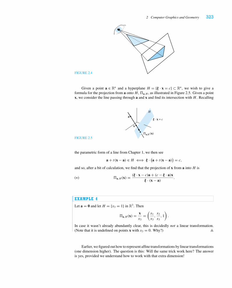
2 Computer Graphics and Geometry 323
FIGURE 2.4
Given a point a ∈ Rn and a hyperplane H = {ξ · x = c} ⊂ Rn, we wish to give aformula for the projection from a onto H , a,H , as illustrated in Figure 2.5. Given a pointx, we consider the line passing through a and x and find its intersection with H . Recalling
FIGURE 2.5
a
x
H
a,H (x)
ξ · x = c
the parametric form of a line from Chapter 1, we then see
a + t (x − a) ∈ H ⇐⇒ ξ · (a + t (x − a)) = c,
and so, after a bit of calculation, we find that the projection of x from a into H is
(∗) a,H (x) = (ξ · x − c)a + (c − ξ · a)xξ · (x − a)
.
EXAMPLE 4
Let a = 0 and let H = {x3 = 1} in R3. Then
a,H (x) = xx3
=(x1
x3,x2
x3, 1
).
In case it wasn’t already abundantly clear, this is decidedly not a linear transformation.(Note that it is undefined on points x with x3 = 0. Why?)
Earlier, we figured out how to represent affine transformations by linear transformations(one dimension higher). The question is this: Will the same trick work here? The answeris yes, provided we understand how to work with that extra dimension!
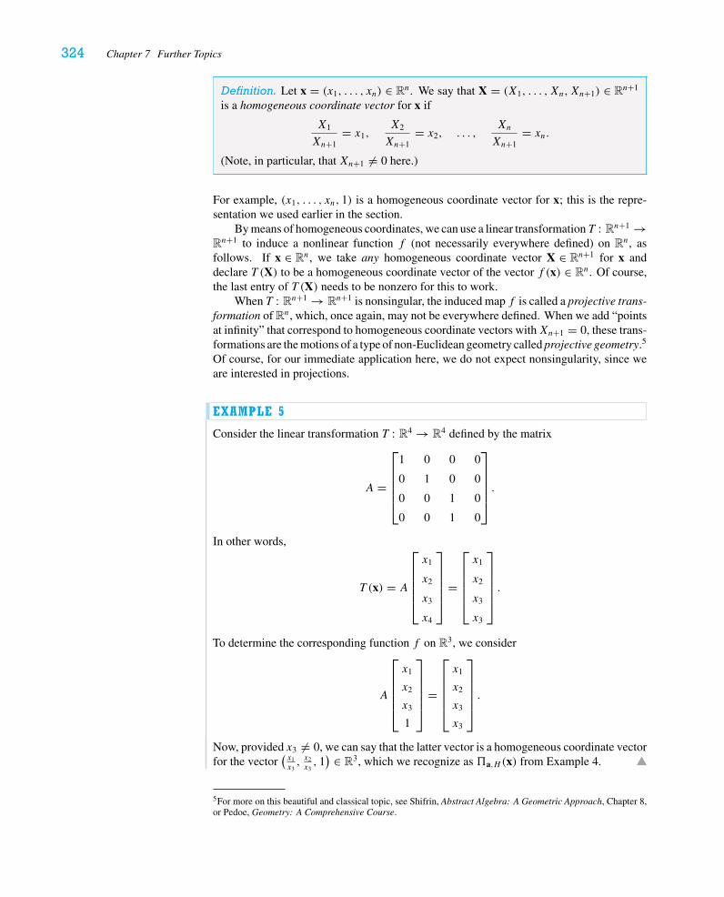
324 Chapter 7 Further Topics
Definition. Let x = (x1, . . . , xn) ∈ Rn. We say that X = (X1, . . . , Xn,Xn+1) ∈ Rn+1
is a homogeneous coordinate vector for x if
X1
Xn+1= x1,
X2
Xn+1= x2, . . . ,
Xn
Xn+1= xn.
(Note, in particular, that Xn+1 �= 0 here.)
For example, (x1, . . . , xn, 1) is a homogeneous coordinate vector for x; this is the repre-sentation we used earlier in the section.
By means of homogeneous coordinates, we can use a linear transformation T : Rn+1 →Rn+1 to induce a nonlinear function f (not necessarily everywhere defined) on Rn, asfollows. If x ∈ Rn, we take any homogeneous coordinate vector X ∈ Rn+1 for x anddeclare T (X) to be a homogeneous coordinate vector of the vector f (x) ∈ Rn. Of course,the last entry of T (X) needs to be nonzero for this to work.
When T : Rn+1 → Rn+1 is nonsingular, the induced map f is called a projective trans-formation of Rn, which, once again, may not be everywhere defined. When we add “pointsat infinity” that correspond to homogeneous coordinate vectors withXn+1 = 0, these trans-formations are the motions of a type of non-Euclidean geometry called projective geometry.5
Of course, for our immediate application here, we do not expect nonsingularity, since weare interested in projections.
EXAMPLE 5
Consider the linear transformation T : R4 → R4 defined by the matrix
A =
⎡⎢⎢⎢⎢⎣
1 0 0 0
0 1 0 0
0 0 1 0
0 0 1 0
⎤⎥⎥⎥⎥⎦.
In other words,
T (x) = A
⎡⎢⎢⎢⎢⎣
x1
x2
x3
x4
⎤⎥⎥⎥⎥⎦
=
⎡⎢⎢⎢⎢⎣
x1
x2
x3
x3
⎤⎥⎥⎥⎥⎦.
To determine the corresponding function f on R3, we consider
A
⎡⎢⎢⎢⎢⎣
x1
x2
x3
1
⎤⎥⎥⎥⎥⎦
=
⎡⎢⎢⎢⎢⎣
x1
x2
x3
x3
⎤⎥⎥⎥⎥⎦.
Now, provided x3 �= 0, we can say that the latter vector is a homogeneous coordinate vectorfor the vector
(x1x3, x2x3, 1) ∈ R3, which we recognize as a,H (x) from Example 4.
5For more on this beautiful and classical topic, see Shifrin, Abstract Algebra: A Geometric Approach, Chapter 8,or Pedoe, Geometry: A Comprehensive Course.
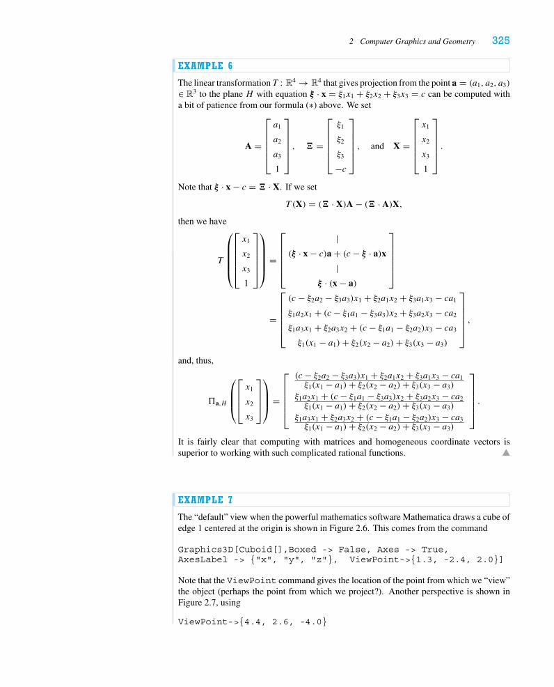
2 Computer Graphics and Geometry 325
EXAMPLE 6
The linear transformation T : R4 → R4 that gives projection from the point a = (a1, a2, a3)
∈ R3 to the plane H with equation ξ · x = ξ1x1 + ξ2x2 + ξ3x3 = c can be computed witha bit of patience from our formula (∗) above. We set
A =
⎡⎢⎢⎢⎢⎣
a1
a2
a3
1
⎤⎥⎥⎥⎥⎦, � =
⎡⎢⎢⎢⎢⎣
ξ1
ξ2
ξ3
−c
⎤⎥⎥⎥⎥⎦, and X =
⎡⎢⎢⎢⎢⎣
x1
x2
x3
1
⎤⎥⎥⎥⎥⎦.
Note that ξ · x − c = � · X. If we set
T (X) = (� · X)A − (� · A)X,
then we have
T
⎛⎜⎜⎜⎜⎝
⎡⎢⎢⎢⎢⎣
x1
x2
x3
1
⎤⎥⎥⎥⎥⎦
⎞⎟⎟⎟⎟⎠
=
⎡⎢⎢⎢⎢⎣
|(ξ · x − c)a + (c − ξ · a)x
|ξ · (x − a)
⎤⎥⎥⎥⎥⎦
=
⎡⎢⎢⎢⎢⎣
(c − ξ2a2 − ξ3a3)x1 + ξ2a1x2 + ξ3a1x3 − ca1
ξ1a2x1 + (c − ξ1a1 − ξ3a3)x2 + ξ3a2x3 − ca2
ξ1a3x1 + ξ2a3x2 + (c − ξ1a1 − ξ2a2)x3 − ca3
ξ1(x1 − a1)+ ξ2(x2 − a2)+ ξ3(x3 − a3)
⎤⎥⎥⎥⎥⎦,
and, thus,
a,H
⎛⎜⎜⎝
⎡⎢⎢⎣x1
x2
x3
⎤⎥⎥⎦
⎞⎟⎟⎠ =
⎡⎢⎢⎢⎢⎣
(c − ξ2a2 − ξ3a3)x1 + ξ2a1x2 + ξ3a1x3 − ca1ξ1(x1 − a1)+ ξ2(x2 − a2)+ ξ3(x3 − a3)
ξ1a2x1 + (c − ξ1a1 − ξ3a3)x2 + ξ3a2x3 − ca2ξ1(x1 − a1)+ ξ2(x2 − a2)+ ξ3(x3 − a3)
ξ1a3x1 + ξ2a3x2 + (c − ξ1a1 − ξ2a2)x3 − ca3ξ1(x1 − a1)+ ξ2(x2 − a2)+ ξ3(x3 − a3)
⎤⎥⎥⎥⎥⎦.
It is fairly clear that computing with matrices and homogeneous coordinate vectors issuperior to working with such complicated rational functions.
EXAMPLE 7
The “default” view when the powerful mathematics software Mathematica draws a cube ofedge 1 centered at the origin is shown in Figure 2.6. This comes from the command
Graphics3D[Cuboid[],Boxed -> False, Axes -> True,AxesLabel -> {"x", "y", "z"}, ViewPoint->{1.3, -2.4, 2.0}]
Note that the ViewPoint command gives the location of the point from which we “view”the object (perhaps the point from which we project?). Another perspective is shown inFigure 2.7, using
ViewPoint->{4.4, 2.6, -4.0}
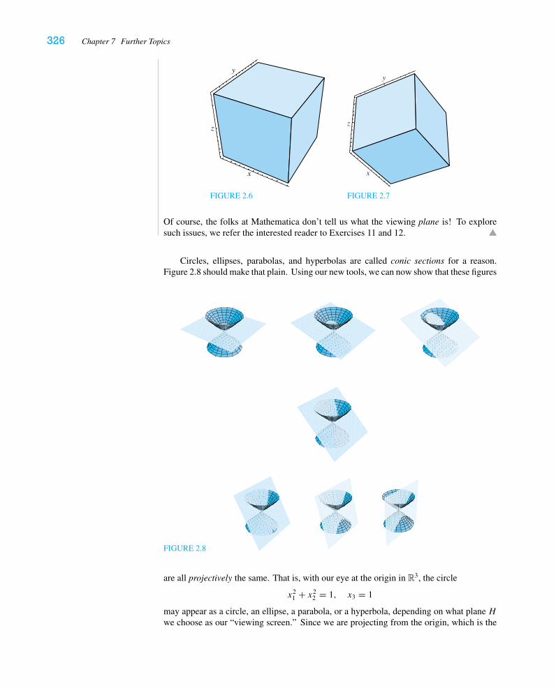
326 Chapter 7 Further Topics
z
x
y
FIGURE 2.6
z
x
y
FIGURE 2.7
Of course, the folks at Mathematica don’t tell us what the viewing plane is! To exploresuch issues, we refer the interested reader to Exercises 11 and 12.
Circles, ellipses, parabolas, and hyperbolas are called conic sections for a reason.Figure 2.8 should make that plain. Using our new tools, we can now show that these figures
FIGURE 2.8
are all projectively the same. That is, with our eye at the origin in R3, the circle
x21 + x2
2 = 1, x3 = 1
may appear as a circle, an ellipse, a parabola, or a hyperbola, depending on what plane Hwe choose as our “viewing screen.” Since we are projecting from the origin, which is the
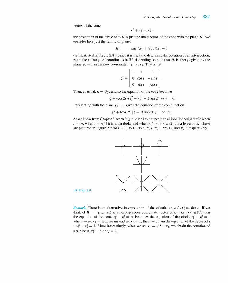
2 Computer Graphics and Geometry 327
vertex of the conex2
1 + x22 = x2
3 ,
the projection of the circle ontoH is just the intersection of the cone with the planeH . Weconsider here just the family of planes
Ht : (− sin t)x2 + (cos t)x3 = 1
(as illustrated in Figure 2.8). Since it is tricky to determine the equation of an intersection,we make a change of coordinates in R3, depending on t , so that Ht is always given by theplane y3 = 1 in the new coordinates y1, y2, y3. That is, let
Q =
⎡⎢⎢⎣
1 0 0
0 cos t − sin t
0 sin t cos t
⎤⎥⎥⎦ .
Then, as usual, x = Qy, and so the equation of the cone becomes
y21 + (cos 2t)(y2
2 − y23)− 2(sin 2t)y2y3 = 0.
Intersecting with the plane y3 = 1 gives the equation of the conic section
y21 + (cos 2t)y2
2 − 2(sin 2t)y2 = cos 2t.
As we know from Chapter 6, when 0 ≤ t < π/4 this curve is an ellipse (indeed, a circle whent = 0), when t = π/4 it is a parabola, and when π/4 < t ≤ π/2 it is a hyperbola. Theseare pictured in Figure 2.9 for t = 0, π/12, π/6, π/4, π/3, 5π/12, and π/2, respectively.
FIGURE 2.9
Remark. There is an alternative interpretation of the calculation we’ve just done. If wethink of X = (x1, x2, x3) as a homogeneous coordinate vector of x = (x1, x2) ∈ R2, thenthe equation of the cone x2
1 + x22 = x2
3 becomes the equation of the circle x21 + x2
2 = 1when we set x3 = 1. If we instead set x2 = 1, then we obtain the equation of the hyperbola−x2
1 + x23 = 1. More interestingly, when we set x3 = √
2 − x2, we obtain the equation ofa parabola, x2
1 − 2√
2x2 = 2.
328 Chapter 7 Further Topics
Exercises 7.2
1. In each case, give the 3 × 3 matrix representing the isometry of R2 and then use youranswer to fit the isometry into our classification scheme.
a.∗ First translate by
[1
1
], and then rotate π/2 about the point (−1, 0).
b.∗ First reflect across the line x1 + x2 = 1, and then translate by
[1
1
].
c. First rotate π/4 about the origin, and then reflect across the line x1 + x2 = 1.
2. Analyze each of the following isometries f : R2 → R2, f (x) = Ax + a (according tothe classification in Theorem 2.4).
a. A =[
0 1
−1 0
], a =
[2
0
]
b.∗ A =[
1 0
0 −1
], a =
[−1
1
]
c. A =[
−1 0
0 1
], a =
[1
0
]
d. A =[
0 1
1 0
], a =
[1
0
]
e. A = 1√2
[1 1
1 −1
], a =
[√2 − 1
1
]
3. Use techniques of linear algebra to find all the isometries of R2 that fix the origin anda.∗ map the x1-axis to itself.
b. map the x1-axis to the x2-axis.
4. Let θ �= 0. Show that
� =
⎡⎢⎢⎣
cos θ − sin θ a1
sin θ cos θ a2
0 0 1
⎤⎥⎥⎦
represents a rotation through angle θ about the point 12
(a1 − a2 cot θ2 , a1 cot θ2 + a2
).
(Hint: To solve for the appropriate eigenvector, you might want to use Cramer’s Rule,Proposition 2.3 of Chapter 5.)
5. Let� =
⎡⎢⎢⎢⎢⎣
|A a
|0 · · · 0 1
⎤⎥⎥⎥⎥⎦
. Prove that the eigenvalues of� consist of the eigenval-
ues of A and 1.
6. Check the details in the proof of Theorem 2.4.
7. Analyze the matrices
⎡⎢⎣
1
0
1
⎤⎥⎦ and
⎡⎢⎢⎢⎣
1
1
0
1
⎤⎥⎥⎥⎦
a. as affine transformations of R2 and R3, respectively.
b. as linear transformations of homogeneous coordinate vectors. From what pointscan we interpret these as perspective projections?
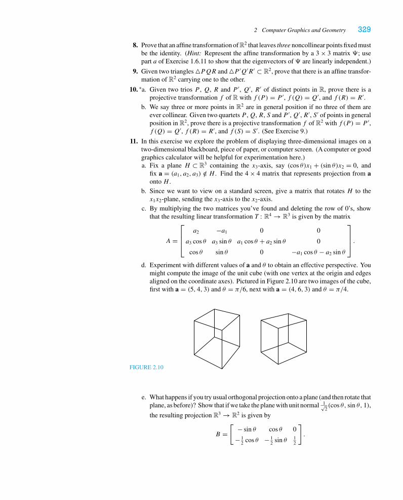
2 Computer Graphics and Geometry 329
8. Prove that an affine transformation of R2 that leaves three noncollinear points fixed mustbe the identity. (Hint: Represent the affine transformation by a 3 × 3 matrix �; usepart a of Exercise 1.6.11 to show that the eigenvectors of � are linearly independent.)
9. Given two triangles �PQR and �P ′Q′R′ ⊂ R2, prove that there is an affine transfor-mation of R2 carrying one to the other.
10. a.∗ Given two trios P , Q, R and P ′, Q′, R′ of distinct points in R, prove there is aprojective transformation f of R with f (P ) = P ′, f (Q) = Q′, and f (R) = R′.
b. We say three or more points in R2 are in general position if no three of them areever collinear. Given two quartets P ,Q, R, S and P ′,Q′, R′, S ′ of points in generalposition in R2, prove there is a projective transformation f of R2 with f (P ) = P ′,f (Q) = Q′, f (R) = R′, and f (S) = S ′. (See Exercise 9.)
11. In this exercise we explore the problem of displaying three-dimensional images on atwo-dimensional blackboard, piece of paper, or computer screen. (A computer or goodgraphics calculator will be helpful for experimentation here.)a. Fix a plane H ⊂ R3 containing the x3-axis, say (cos θ)x1 + (sin θ)x2 = 0, and
fix a = (a1, a2, a3) /∈ H . Find the 4 × 4 matrix that represents projection from aonto H .
b. Since we want to view on a standard screen, give a matrix that rotates H to thex1x2-plane, sending the x3-axis to the x2-axis.
c. By multiplying the two matrices you’ve found and deleting the row of 0’s, showthat the resulting linear transformation T : R4 → R3 is given by the matrix
A =
⎡⎢⎢⎣
a2 −a1 0 0
a3 cos θ a3 sin θ a1 cos θ + a2 sin θ 0
cos θ sin θ 0 −a1 cos θ − a2 sin θ
⎤⎥⎥⎦ .
d. Experiment with different values of a and θ to obtain an effective perspective. Youmight compute the image of the unit cube (with one vertex at the origin and edgesaligned on the coordinate axes). Pictured in Figure 2.10 are two images of the cube,first with a = (5, 4, 3) and θ = π/6, next with a = (4, 6, 3) and θ = π/4.
FIGURE 2.10
e. What happens if you try usual orthogonal projection onto a plane (and then rotate thatplane, as before)? Show that if we take the plane with unit normal 1√
2(cos θ, sin θ, 1),
the resulting projection R3 → R2 is given by
B =[
− sin θ cos θ 0
− 12 cos θ − 1
2 sin θ 12
].
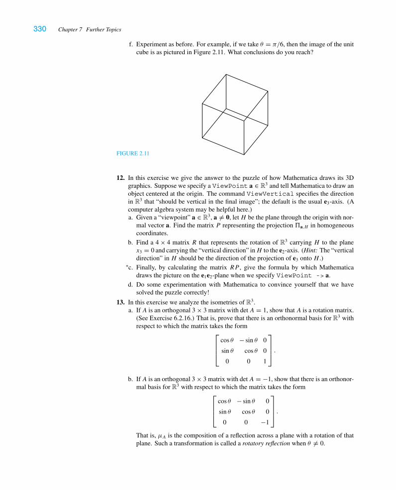
330 Chapter 7 Further Topics
f. Experiment as before. For example, if we take θ = π/6, then the image of the unitcube is as pictured in Figure 2.11. What conclusions do you reach?
FIGURE 2.11
12. In this exercise we give the answer to the puzzle of how Mathematica draws its 3Dgraphics. Suppose we specify a ViewPoint a ∈ R3 and tell Mathematica to draw anobject centered at the origin. The command ViewVertical specifies the directionin R3 that “should be vertical in the final image”; the default is the usual e3-axis. (Acomputer algebra system may be helpful here.)a. Given a “viewpoint” a ∈ R3, a �= 0, letH be the plane through the origin with nor-
mal vector a. Find the matrix P representing the projection a,H in homogeneouscoordinates.
b. Find a 4 × 4 matrix R that represents the rotation of R3 carrying H to the planex3 = 0 and carrying the “vertical direction” inH to the e2-axis. (Hint: The “verticaldirection” in H should be the direction of the projection of e3 onto H .)
c.∗ Finally, by calculating the matrix RP , give the formula by which Mathematicadraws the picture on the e1e2-plane when we specify ViewPoint -> a.
d. Do some experimentation with Mathematica to convince yourself that we havesolved the puzzle correctly!
13. In this exercise we analyze the isometries of R3.a. If A is an orthogonal 3 × 3 matrix with detA = 1, show that A is a rotation matrix.
(See Exercise 6.2.16.) That is, prove that there is an orthonormal basis for R3 withrespect to which the matrix takes the form
⎡⎢⎢⎣
cos θ − sin θ 0
sin θ cos θ 0
0 0 1
⎤⎥⎥⎦ .
b. IfA is an orthogonal 3 × 3 matrix with detA = −1, show that there is an orthonor-mal basis for R3 with respect to which the matrix takes the form
⎡⎢⎢⎣
cos θ − sin θ 0
sin θ cos θ 0
0 0 −1
⎤⎥⎥⎦ .
That is, μA is the composition of a reflection across a plane with a rotation of thatplane. Such a transformation is called a rotatory reflection when θ �= 0.
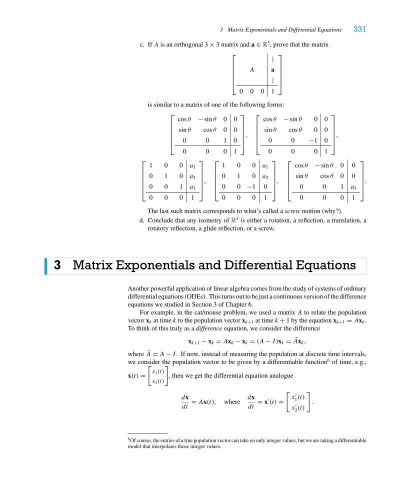
3 Matrix Exponentials and Differential Equations 331
c. If A is an orthogonal 3 × 3 matrix and a ∈ R3, prove that the matrix⎡⎢⎢⎢⎢⎣
|A a
|0 0 0 1
⎤⎥⎥⎥⎥⎦
is similar to a matrix of one of the following forms:⎡⎢⎢⎢⎢⎣
cos θ − sin θ 0 0
sin θ cos θ 0 0
0 0 1 0
0 0 0 1
⎤⎥⎥⎥⎥⎦,
⎡⎢⎢⎢⎢⎣
cos θ − sin θ 0 0
sin θ cos θ 0 0
0 0 −1 0
0 0 0 1
⎤⎥⎥⎥⎥⎦,
⎡⎢⎢⎢⎢⎣
1 0 0 a1
0 1 0 a2
0 0 1 a3
0 0 0 1
⎤⎥⎥⎥⎥⎦,
⎡⎢⎢⎢⎢⎣
1 0 0 a1
0 1 0 a2
0 0 −1 0
0 0 0 1
⎤⎥⎥⎥⎥⎦,
⎡⎢⎢⎢⎢⎣
cos θ − sin θ 0 0
sin θ cos θ 0 0
0 0 1 a3
0 0 0 1
⎤⎥⎥⎥⎥⎦.
The last such matrix corresponds to what’s called a screw motion (why?).
d. Conclude that any isometry of R3 is either a rotation, a reflection, a translation, arotatory reflection, a glide reflection, or a screw.
3 Matrix Exponentials and Differential Equations
Another powerful application of linear algebra comes from the study of systems of ordinarydifferential equations (ODEs). This turns out to be just a continuous version of the differenceequations we studied in Section 3 of Chapter 6.
For example, in the cat/mouse problem, we used a matrix A to relate the populationvector xk at time k to the population vector xk+1 at time k + 1 by the equation xk+1 = Axk .To think of this truly as a difference equation, we consider the difference
xk+1 − xk = Axk − xk = (A− I )xk = Axk,
where A = A− I . If now, instead of measuring the population at discrete time intervals,we consider the population vector to be given by a differentiable function6 of time, e.g.,
x(t) =[x1(t)
x2(t)
], then we get the differential equation analogue
dxdt
= Ax(t), wheredxdt
= x′(t) =[x ′
1(t)
x ′2(t)
].
6Of course, the entries of a true population vector can take on only integer values, but we are taking a differentiablemodel that interpolates those integer values.
332 Chapter 7 Further Topics
We can rewrite this as a system of linear differential equations:
dx1
dt= a11x1(t)+ a12x2(t)
dx2
dt= a21x1(t)+ a22x2(t).
In this case, the coefficients aij are independent of t , and so we call this a constant-coefficientsystem of ODEs.
The main problem we address in this section is the following. Given ann× n (constant)matrix A and a vector x0 ∈ Rn, we wish to find all differentiable vector-valued functionsx(t) so that
dxdt
= Ax(t), x(0) = x0.
(The vector x0 is called the initial value of the solution x(t).)
EXAMPLE 1
Suppose n = 1, so thatA = [a] for some real number a. Then we have simply the ordinarydifferential equation
dx
dt= ax(t), x(0) = x0.
The trick of “separating variables” that the reader probably learned in her integral calculuscourse leads to the solution7
dx
dt= ax(t)
dx
x= a dt
∫dx
x=∫a dt
ln |x| = at + cx(t) = Ceat (where we have set C = ±ec).
Using the fact that x(0) = x0, we find that C = x0 and so the solution is
x(t) = x0eat .
As we can easily check, dxdt
= ax(t), so we have in fact found a solution. Do we knowthere can be no more? Suppose y(t) were any solution of the original problem. Then thefunction z(t) = y(t)e−at satisfies the equation
dz
dt= dy
dte−at + y(t) (−ae−at) = (ay(t)) e−at + y(t) (−ae−at) = 0,
and so z(t)must be a constant function. Since z(0) = y(0) = x0, we see that y(t) = x0eat .
The original differential equation (with its initial condition) has a unique solution.
7If the formal manipulation makes you feel uneasy, then use the chain rule to notice that 1x(t)
dxdt
= ddt
ln |x(t)|.
3 Matrix Exponentials and Differential Equations 333
EXAMPLE 2
Consider perhaps the simplest possible 2 × 2 example:
dx1
dt= ax1(t)
dx2
dt= bx2(t)
with the initial conditions x1(0) = (x1)0, x2(0) = (x2)0. In matrix notation, this is the ODE
dxdt
= Ax(t), x(0) = x0, where
A =[a 0
0 b
], x(t) =
[x1(t)
x2(t)
], and x0 =
[(x1)0
(x2)0
].
Since x1(t) and x2(t) appear completely independently in these equations, we infer fromExample 1 that the unique solution of this system of equations will be
x1(t) = (x1)0eat , x2(t) = (x2)0e
bt .
In vector notation, we have
x(t) =[x1(t)
x2(t)
]=[eat 0
0 ebt
]x0 = E(t)x0,
where E(t) is the diagonal 2 × 2 matrix with entries eat and ebt . This result is easilygeneralized to the case of a diagonal n× n matrix.
Before moving on to more complicated examples, we introduce some notation. Re-member that for any positive integer k, the symbol k!, read “k factorial,” denotes the productk! = 1 · 2 · · · · · (k − 1) · k. By convention, 0! is defined to be 1. We also recall that for anyreal number x,
(†) ex =∞∑k=0
xk
k! = 1 + x + 1
2x2 + 1
6x3 + · · · + 1
k!xk + . . .
(see Exercise 15). Now, given an n× nmatrix A, we define a new n× nmatrix eA, calledthe exponential of A, by the “power series”
eA = I + A+ 1
2A2 + 1
6A3 + · · · + 1
k!Ak + . . . =
∞∑k=0
Ak
k! .
In general, trying to compute this series directly is extremely difficult, because the coeffi-cients of Ak are not easily expressed in terms of the coefficients of A; indeed, it is not at allobvious that this power series will converge (but see Exercise 16). However, when A is adiagonal matrix, it is easy to compute eA, because we know that if
A =
⎡⎢⎢⎢⎢⎣
λ1
λ2
. . .
λn
⎤⎥⎥⎥⎥⎦, then Ak =
⎡⎢⎢⎢⎢⎣
λk1
λk2. . .
λkn
⎤⎥⎥⎥⎥⎦,
334 Chapter 7 Further Topics
and so eA will likewise be diagonal, with its i th diagonal entry∞∑k=0
λki
k! = eλi .
That is,
if A =
⎡⎢⎢⎢⎢⎣
λ1
λ2
. . .
λn
⎤⎥⎥⎥⎥⎦, then eA =
⎡⎢⎢⎢⎢⎣
eλ1
eλ2
. . .
eλn
⎤⎥⎥⎥⎥⎦.
Using this notation, we see that the matrix E(t) that appeared in Example 2 above is justthe matrix etA.
Indeed, when A is diagonalizable, there is an invertible matrix P so that� = P−1AP
is diagonal. Thus, A = P�P−1 and Ak = P�kP−1 for all positive integers k, and so
eA =∞∑k=0
Ak
k! =∞∑k=0
P�kP−1
k! = P
( ∞∑k=0
�k
k!
)P−1 = Pe�P−1.
EXAMPLE 3
Let A =[
2 0
3 −1
]. Then A = P�P−1, where
� =[
2
−1
]and P =
[1 0
1 1
].
Then we have
et� =[e2t
e−t
]and etA = Pet�P−1 =
[e2t 0
e2t − e−t e−t
].
When A(t) is a matrix-valued function of t—or, if you prefer, a matrix whose en-tries are functions aij (t)—we define the derivative, just as for vector functions above, bydifferentiating entry by entry:8
dA
dt= A′(t) = [a′
ij (t)].
The result of Example 2 generalizes to the n× n case. Indeed, as we saw in Chapter 6,whenever we can solve a problem for diagonal matrices, we can solve it for diagonalizablematrices by making the appropriate change of basis. So we should not be surprised by thefollowing result.
8Not surprisingly, many of the usual rules of calculus have analogous matrix formulations, provided one is carefulabout the order of multiplication. For example, if A(t) and B(t) are matrices whose entries are differentiablefunctions of t , then d
dt(A(t)B(t)) = A′(t)B(t)+ A(t)B ′(t). One can prove this entry by entry, but it is more
insightful to writeA′(t) = limh→0
(A(t + h)− A(t))/h and use the usual proof of the product rule from first-semester
calculus.
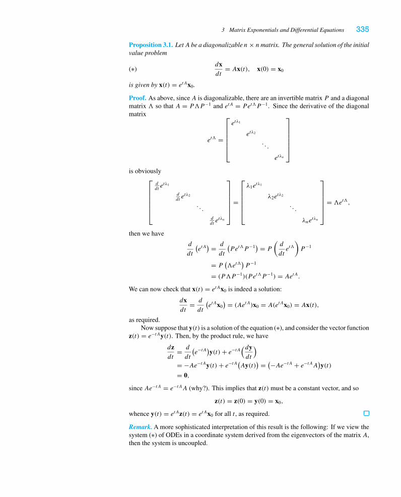
3 Matrix Exponentials and Differential Equations 335
Proposition 3.1. LetA be a diagonalizable n× nmatrix. The general solution of the initialvalue problem
(∗)dxdt
= Ax(t), x(0) = x0
is given by x(t) = etAx0.
Proof. As above, since A is diagonalizable, there are an invertible matrix P and a diagonalmatrix � so that A = P�P−1 and etA = Pet�P−1. Since the derivative of the diagonalmatrix
et� =
⎡⎢⎢⎢⎢⎢⎣
etλ1
etλ2
. . .
etλn
⎤⎥⎥⎥⎥⎥⎦
is obviously⎡⎢⎢⎢⎢⎢⎣
ddtetλ1
ddtetλ2
. . .
ddtetλn
⎤⎥⎥⎥⎥⎥⎦
=
⎡⎢⎢⎢⎢⎢⎣
λ1etλ1
λ2etλ2
. . .
λnetλn
⎤⎥⎥⎥⎥⎥⎦
= �et�,
then we have
d
dt
(etA) = d
dt
(Pet�P−1
) = P
(d
dtet�)P−1
= P(�et�
)P−1
= (P�P−1)(P et�P−1) = AetA.
We can now check that x(t) = etAx0 is indeed a solution:
dxdt
= d
dt
(etAx0
) = (AetA)x0 = A(etAx0) = Ax(t),
as required.Now suppose that y(t) is a solution of the equation (∗), and consider the vector function
z(t) = e−tAy(t). Then, by the product rule, we have
dzdt
= d
dt
(e−tA)y(t)+ e−tA
(dydt
)
= −Ae−tAy(t)+ e−tA(Ay(t)) = (−Ae−tA + e−tAA)y(t)
= 0,
since Ae−tA = e−tAA (why?). This implies that z(t) must be a constant vector, and so
z(t) = z(0) = y(0) = x0,
whence y(t) = etAz(t) = etAx0 for all t , as required.
Remark. A more sophisticated interpretation of this result is the following: If we view thesystem (∗) of ODEs in a coordinate system derived from the eigenvectors of the matrix A,then the system is uncoupled.
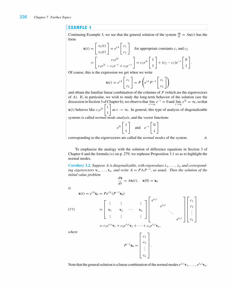
336 Chapter 7 Further Topics
EXAMPLE 4
Continuing Example 3, we see that the general solution of the system dxdt
= Ax(t) has theform
x(t) =[x1(t)
x2(t)
]= etA
[c1
c2
]for appropriate constants c1 and c2
=[
c1e2t
c1e2t − c1e
−t + c2e−t
]= c1e
2t
[1
1
]+ (c2 − c1)e
−t[
0
1
].
Of course, this is the expression we get when we write
x(t) = etA
[c1
c2
]= P
(et�P−1
[c1
c2
])
and obtain the familiar linear combination of the columns of P (which are the eigenvectorsof A). If, in particular, we wish to study the long-term behavior of the solution (see thediscussion in Section 3 of Chapter 6), we observe that lim
t→∞ e−t = 0 and lim
t→∞ e2t = ∞, so that
x(t) behaves like c1e2t
[1
1
]as t → ∞. In general, this type of analysis of diagonalizable
systems is called normal mode analysis, and the vector functions
e2t
[1
1
]and e−t
[0
1
]
corresponding to the eigenvectors are called the normal modes of the system.
To emphasize the analogy with the solution of difference equations in Section 3 ofChapter 6 and the formula (∗) on p. 279, we rephrase Proposition 3.1 so as to highlight thenormal modes.
Corollary 3.2. Suppose A is diagonalizable, with eigenvalues λ1, . . . , λn and correspond-ing eigenvectors v1, . . . , vn, and write A = P�P−1, as usual. Then the solution of theinitial value problem
dxdt
= Ax(t), x(0) = x0
is
x(t) = etAx0 = Pet�(P−1x0)
=
⎡⎢⎢⎣
|v1
|
|v2
|· · ·
|vn
|
⎤⎥⎥⎦
⎡⎢⎢⎢⎢⎢⎣
eλ1t
eλ2t
. . .
eλnt
⎤⎥⎥⎥⎥⎥⎦
⎡⎢⎢⎢⎢⎢⎣
c1
c2...
cn
⎤⎥⎥⎥⎥⎥⎦
(††)
= c1eλ1tv1 + c2e
λ2tv2 + · · · + cneλntvn,where
P−1x0 =
⎡⎢⎢⎢⎢⎢⎣
c1
c2...
cn
⎤⎥⎥⎥⎥⎥⎦.
Note that the general solution is a linear combination of the normal modes eλ1tv1, . . . , eλntvn.
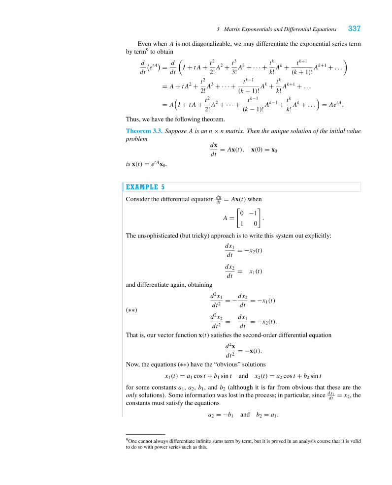
3 Matrix Exponentials and Differential Equations 337
Even when A is not diagonalizable, we may differentiate the exponential series termby term9 to obtain
d
dt
(etA) = d
dt
(I + tA+ t2
2!A2 + t3
3!A3 + · · · + tk
k!Ak + tk+1
(k + 1)!Ak+1 + . . .
)
= A+ tA2 + t2
2!A3 + · · · + tk−1
(k − 1)!Ak + tk
k!Ak+1 + . . .
= A(I + tA+ t2
2!A2 + · · · + tk−1
(k − 1)!Ak−1 + tk
k!Ak + . . .
)= AetA.
Thus, we have the following theorem.
Theorem 3.3. Suppose A is an n× n matrix. Then the unique solution of the initial valueproblem
dxdt
= Ax(t), x(0) = x0
is x(t) = etAx0.
EXAMPLE 5
Consider the differential equation dxdt
= Ax(t) when
A =[
0 −1
1 0
].
The unsophisticated (but tricky) approach is to write this system out explicitly:
dx1
dt= −x2(t)
dx2
dt= x1(t)
and differentiate again, obtaining
d2x1
dt2= −dx2
dt= −x1(t)
(∗∗)d2x2
dt2= dx1
dt= −x2(t).
That is, our vector function x(t) satisfies the second-order differential equation
d2xdt2
= −x(t).
Now, the equations (∗∗) have the “obvious” solutions
x1(t) = a1 cos t + b1 sin t and x2(t) = a2 cos t + b2 sin t
for some constants a1, a2, b1, and b2 (although it is far from obvious that these are theonly solutions). Some information was lost in the process; in particular, since dx1
dt= x2, the
constants must satisfy the equations
a2 = −b1 and b2 = a1.
9One cannot always differentiate infinite sums term by term, but it is proved in an analysis course that it is validto do so with power series such as this.
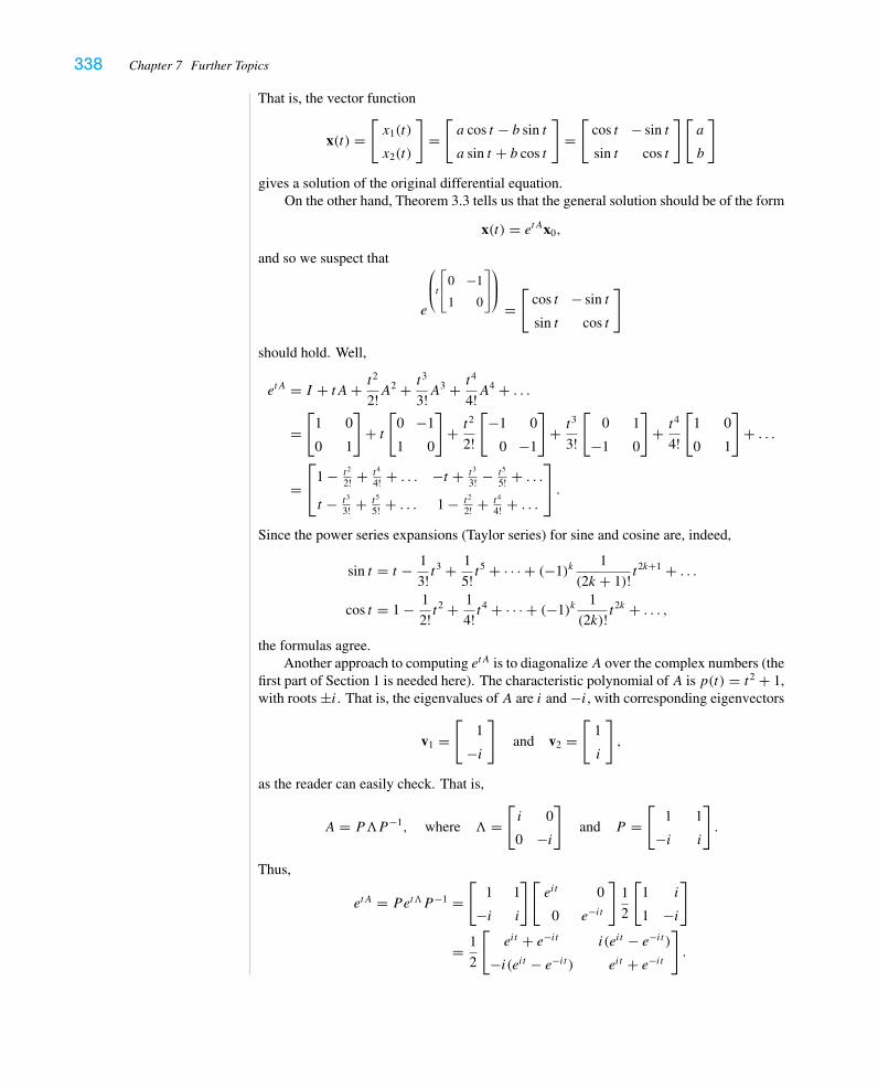
338 Chapter 7 Further Topics
That is, the vector function
x(t) =[x1(t)
x2(t)
]=[a cos t − b sin t
a sin t + b cos t
]=[
cos t − sin t
sin t cos t
][a
b
]
gives a solution of the original differential equation.On the other hand, Theorem 3.3 tells us that the general solution should be of the form
x(t) = etAx0,
and so we suspect that
e
⎛⎜⎝t
⎡⎢⎣
0 −1
1 0
⎤⎥⎦
⎞⎟⎠
=[
cos t − sin t
sin t cos t
]
should hold. Well,
etA = I + tA+ t2
2!A2 + t3
3!A3 + t4
4!A4 + . . .
=[
1 0
0 1
]+ t[
0 −1
1 0
]+ t2
2!
[−1 0
0 −1
]+ t3
3!
[0 1
−1 0
]+ t4
4!
[1 0
0 1
]+ . . .
=⎡⎣1 − t2
2! + t4
4! + . . . −t + t3
3! − t5
5! + . . .t − t3
3! + t5
5! + . . . 1 − t2
2! + t4
4! + . . .
⎤⎦ .
Since the power series expansions (Taylor series) for sine and cosine are, indeed,
sin t = t − 1
3! t3 + 1
5! t5 + · · · + (−1)k
1
(2k + 1)! t2k+1 + . . .
cos t = 1 − 1
2! t2 + 1
4! t4 + · · · + (−1)k
1
(2k)! t2k + . . . ,
the formulas agree.Another approach to computing etA is to diagonalizeA over the complex numbers (the
first part of Section 1 is needed here). The characteristic polynomial of A is p(t) = t2 + 1,with roots ±i. That is, the eigenvalues of A are i and −i, with corresponding eigenvectors
v1 =[
1
−i
]and v2 =
[1
i
],
as the reader can easily check. That is,
A = P�P−1, where � =[i 0
0 −i
]and P =
[1 1
−i i
].
Thus,
etA = Pet�P−1 =[
1 1
−i i
][eit 0
0 e−it
]1
2
[1 i
1 −i
]
= 1
2
[eit + e−it i(eit − e−it )
−i(eit − e−it ) eit + e−it].
3 Matrix Exponentials and Differential Equations 339
Now comes one of the great mathematical relationships of all time, the discovery of whichis usually attributed to Euler:10 If we substitute it for x in the equation (†) on p. 333, we tobtain
eit =∞∑k=0
(it)k
k! = 1 + it − 1
2! t2 − i 1
3! t3 + 1
4! t4 + . . .
=(
1 − 1
2! t2 + 1
4! t4 + . . .
)+ i(t − 1
3! t3 + 1
5! t5 + . . .
)= cos t + i sin t.
Then it follows immediately that
etA = 1
2
[eit + e−it i(eit − e−it )
−i(eit − e−it ) eit + e−it]
=[
cos t − sin t
sin t cos t
],
exactly as before.
EXAMPLE 6
Consider the matrix
A =[
1 2
−2 1
],
whose characteristic polynomial is p(t) = t2 − 2t + 5. Thus, the eigenvalues of A are1 ± 2i, with respective eigenvectors
v1 =[
1
i
]and v2 =
[1
−i
].
The general solution of the differential equation dxdt
= Ax is given by
x(t) = c1e(1+2i)t
[1
i
]+ c2e
(1−2i)t
[1
−i
]
= c1et (cos 2t + i sin 2t)
[1
i
]+ c2e
t (cos 2t − i sin 2t)
[1
−i
],
and, separating this expression into its real and imaginary parts, we obtain
= (c1 + c2)et
[cos 2t
− sin 2t
]+ i(c1 − c2)e
t
[sin 2t
cos 2t
]
= et
[cos 2t sin 2t
− sin 2t cos 2t
][c1 + c2
i(c1 − c2)
].
10Although Euler published this in 1743, the result was apparently first discovered by Cotes in 1714. See Maor,e: The Story of a Number.
340 Chapter 7 Further Topics
Since the matrixA is real, the real and imaginary parts of x(t)must be solutions, and indeed,the general solution is a linear combination of the normal modes
et
[cos 2t
− sin 2t
]and et
[sin 2t
cos 2t
].
Solution curves are spirals emanating from the origin (as t → −∞) with exponentiallyincreasing radius.
EXAMPLE 7
Let’s now consider the case of a non-diagonalizable matrix, such as
A =[
2 1
0 2
].
The system
dx1
dt= 2x1 + x2
dx2
dt= 2x2
is already partially uncoupled, so we know that x2(t) must take the form x2(t) = ce2t forsome constant c. Now, in order to find x1(t), we must solve the inhomogeneous ODE
dx1
dt= 2x1(t)+ ce2t .
In elementary differential equations courses, one is taught to look for a solution of the form
x1(t) = ae2t + bte2t ;in this case,
dx1
dt= (2a + b)e2t + (2b)te2t = 2x1(t)+ be2t ,
and so taking b = c gives the desired solution to our equation. That is, the solution to thesystem is the vector function
x(t) =[ae2t + cte2t
ce2t
]=[e2t te2t
0 e2t
][a
c
].
The explanation of the trick is quite simple. Let’s calculate the matrix exponential etA
by writing
A =[
2 0
0 2
]+[
0 1
0 0
]= 2I + B, where B =
[0 1
0 0
].
The powers of A are easy to compute because B2 = 0: By the binomial theorem (seeExercise 2.1.15),
(2I + B)k = 2kI + k2k−1B,
3 Matrix Exponentials and Differential Equations 341
and so
etA =∞∑k=0
tk
k!Ak =
∞∑k=0
tk
k!(2kI + k2k−1B
)
=∞∑k=0
(2t)k
k! I +∞∑k=0
tk
k!(k2k−1
)B
= e2t I + t∞∑k=1
(2t)k−1
(k − 1)!B = e2t I + t∞∑k=0
(2t)k
k! B
= e2t I + te2tB =[e2t te2t
0 e2t
].
A similar phenomenon occurs with any matrix in Jordan canonical form (see Exercises 4and 8).
Let’s consider the general nth-order linear ODE with constant coefficients:
(�) y(n)(t)+ an−1y(n−1)(t)+ · · · + a2y
′′(t)+ a1y′(t)+ a0y(t) = 0.
Here a0, a1, . . . , an−1 are scalars, and y(t) is assumed to be n-times differentiable; y(k)(t)denotes its kth derivative. We can use the power of Theorem 3.3 to derive the followinggeneral result. (See Section 6 of Chapter 3 for a discussion of the vector space C∞(I) ofinfinitely differentiable functions on an interval I.)
Theorem 3.4. Let n be a positive integer. The set of solutions of the nth-order ODE (�) isan n-dimensional subspace of C∞(R), the vector space of infinitely differentiable functionsdefined on R. In particular, the initial value problem
y(n)(t)+ an−1y(n−1)(t)+ · · · + a2y
′′(t)+ a1y′(t)+ a0y(t) = 0
y(0) = c0, y ′(0) = c1, y ′′(0) = c2, . . . , y(n−1)(0) = cn−1
has a unique solution.
Proof. The trick is to concoct a way to apply Theorem 3.3. We introduce the vector functionx(t) defined by
x(t) =
⎡⎢⎢⎢⎢⎢⎢⎢⎢⎣
y(t)
y ′(t)y ′′(t)...
y(n−1)(t)
⎤⎥⎥⎥⎥⎥⎥⎥⎥⎦
and observe that it satisfies the first-order system of ODEs
dxdt
=
⎡⎢⎢⎢⎢⎢⎢⎢⎢⎣
y ′(t)y ′′(t)y ′′′(t)...
y(n)(t)
⎤⎥⎥⎥⎥⎥⎥⎥⎥⎦
=
⎡⎢⎢⎢⎢⎢⎢⎢⎢⎣
0 1 0 · · · 0
0 0 1 · · · 0
0 0 0. . . 0
......
.... . .
...
−a0 −a1 −a2 · · · −an−1
⎤⎥⎥⎥⎥⎥⎥⎥⎥⎦
⎡⎢⎢⎢⎢⎢⎢⎢⎢⎣
y(t)
y ′(t)y ′′(t)...
y(n−1)(t)
⎤⎥⎥⎥⎥⎥⎥⎥⎥⎦
= Ax(t),
342 Chapter 7 Further Topics
where A is the obvious matrix of coefficients. We infer from Theorem 3.3 that the generalsolution is x(t) = etAx0, so
⎡⎢⎢⎢⎢⎢⎢⎢⎢⎣
y(t)
y ′(t)y ′′(t)...
y(n−1)(t)
⎤⎥⎥⎥⎥⎥⎥⎥⎥⎦
= etA
⎡⎢⎢⎢⎢⎢⎢⎢⎢⎣
c0
c1
c2
...
cn−1
⎤⎥⎥⎥⎥⎥⎥⎥⎥⎦
= c0v1(t)+ c1v2(t)+ · · · + cn−1vn(t),
where vj (t) are the columns of etA. In particular, if we let q1(t), . . . , qn(t) denote the firstentries of the vector functions v1(t), . . . , vn(t), respectively, we see that
y(t) = c0q1(t)+ c1q2(t)+ · · · + cn−1qn(t);that is, the functions q1, . . . , qn span the vector space of solutions of the differential equation(�). Note that these functions are infinitely differentiable since the entries of etA are. Last,we claim that these functions are linearly independent. Suppose that for some scalarsc0, c1, . . . , cn−1, we have
y(t) = c0q1(t)+ c1q2(t)+ · · · + cn−1qn(t) = 0 for all t.
Then, differentiating, we have the same linear relation among all of the kth derivatives ofq1, . . . , qn, for k = 1, . . . , n− 1, and so we have
etA
⎡⎢⎢⎢⎢⎢⎢⎢⎢⎣
c0
c1
c2
...
cn−1
⎤⎥⎥⎥⎥⎥⎥⎥⎥⎦
= c0v1(t)+ c1v2(t)+ · · · + cn−1vn(t) = 0.
Since etA is an invertible matrix (see Exercise 13), we infer that c0 = c1 = · · · = cn−1 = 0,and so {q1, . . . , qn} is linearly independent.
EXAMPLE 8
Let
A =[−3 2
2 −3
],
and consider the second -order system of ODEs
d2xdt2
= Ax, x(0) = x0,dxdt(0) = x′
0.
The experience we gained in Example 5 suggests that if we can uncouple this system (byfinding eigenvalues and eigenvectors), we should expect to find normal modes that aresinusoidal in nature.
The characteristic polynomial of A is p(t) = t2 + 6t + 5, and so its eigenvalues areλ1 = −1 and λ2 = −5, with corresponding eigenvectors
v1 =[
1
1
]and v2 =
[1
−1
].
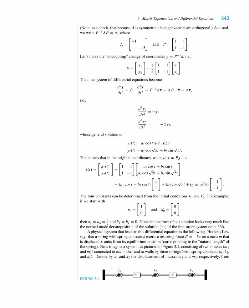
3 Matrix Exponentials and Differential Equations 343
(Note, as a check, that because A is symmetric, the eigenvectors are orthogonal.) As usual,we write P−1AP = �, where
� =[−1
−5
]and P =
[1 1
1 −1
].
Let’s make the “uncoupling” change of coordinates y = P−1x, i.e.,
y =[y1
y2
]= 1
2
[1 1
1 −1
][x1
x2
].
Then the system of differential equations becomes
d2ydt2
= P−1 d2xdt2
= P−1Ax = �P−1x = �y,
i.e.,
d2y1
dt2= −y1
d2y2
dt2= − 5y2,
whose general solution is
y1(t) = a1 cos t + b1 sin t
y2(t) = a2 cos√
5t + b2 sin√
5t.
This means that in the original coordinates, we have x = Py, i.e.,
x(t) =[x1(t)
x2(t)
]=[
1 1
1 −1
][a1 cos t + b1 sin t
a2 cos√
5t + b2 sin√
5t
]
= (a1 cos t + b1 sin t)
[1
1
]+ (a2 cos
√5t + b2 sin
√5t)
[1
−1
].
The four constants can be determined from the initial conditions x0 and x′0. For example,
if we start with
x0 =[
1
0
]and x′
0 =[
0
0
],
then a1 = a2 = 12 and b1 = b2 = 0. Note that the form of our solution looks very much like
the normal mode decomposition of the solution (††) of the first-order system on p. 336.A physical system that leads to this differential equation is the following. Hooke’s Law
says that a spring with spring constant k exerts a restoring force F = −kx on a massm thatis displaced x units from its equilibrium position (corresponding to the “natural length” ofthe spring). Now imagine a system, as pictured in Figure 3.1, consisting of two masses (m1
andm2) connected to each other and to walls by three springs (with spring constants k1, k2,and k3). Denote by x1 and x2 the displacement of masses m1 and m2, respectively, from
FIGURE 3.1
k1 k3k2m2m1
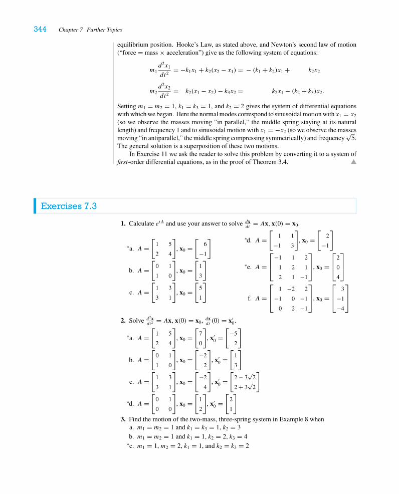
344 Chapter 7 Further Topics
equilibrium position. Hooke’s Law, as stated above, and Newton’s second law of motion(“force = mass × acceleration”) give us the following system of equations:
m1d2x1
dt2= −k1x1 + k2(x2 − x1) = − (k1 + k2)x1 + k2x2
m2d2x2
dt2= k2(x1 − x2)− k3x2 = k2x1 − (k2 + k3)x2.
Setting m1 = m2 = 1, k1 = k3 = 1, and k2 = 2 gives the system of differential equationswith which we began. Here the normal modes correspond to sinusoidal motion with x1 = x2
(so we observe the masses moving “in parallel,” the middle spring staying at its naturallength) and frequency 1 and to sinusoidal motion with x1 = −x2 (so we observe the massesmoving “in antiparallel,” the middle spring compressing symmetrically) and frequency
√5.
The general solution is a superposition of these two motions.In Exercise 11 we ask the reader to solve this problem by converting it to a system of
first-order differential equations, as in the proof of Theorem 3.4.
Exercises 7.3
1. Calculate etA and use your answer to solve dxdt
= Ax, x(0) = x0.
a.∗ A =[
1 5
2 4
], x0 =
[6
−1
]
b. A =[
0 1
1 0
], x0 =
[1
3
]
c. A =[
1 3
3 1
], x0 =
[5
1
]
d.∗ A =[
1 1
−1 3
], x0 =
[2
−1
]
e.∗ A =⎡⎢⎣
−1 1 2
1 2 1
2 1 −1
⎤⎥⎦, x0 =
⎡⎢⎣
2
0
4
⎤⎥⎦
f. A =⎡⎢⎣
1 −2 2
−1 0 −1
0 2 −1
⎤⎥⎦, x0 =
⎡⎢⎣
3
−1
−4
⎤⎥⎦
2. Solve d2xdt2
= Ax, x(0) = x0, dxdt(0) = x′
0.
a.∗ A =[
1 5
2 4
], x0 =
[7
0
], x′
0 =[
−5
2
]
b. A =[
0 1
1 0
], x0 =
[−2
2
], x′
0 =[
1
3
]
c. A =[
1 3
3 1
], x0 =
[−2
4
], x′
0 =[
2 − 3√
2
2 + 3√
2
]
d.∗ A =[
0 1
0 0
], x0 =
[1
2
], x′
0 =[
2
1
]
3. Find the motion of the two-mass, three-spring system in Example 8 whena. m1 = m2 = 1 and k1 = k3 = 1, k2 = 3
b. m1 = m2 = 1 and k1 = 1, k2 = 2, k3 = 4
c.∗ m1 = 1, m2 = 2, k1 = 1, and k2 = k3 = 2
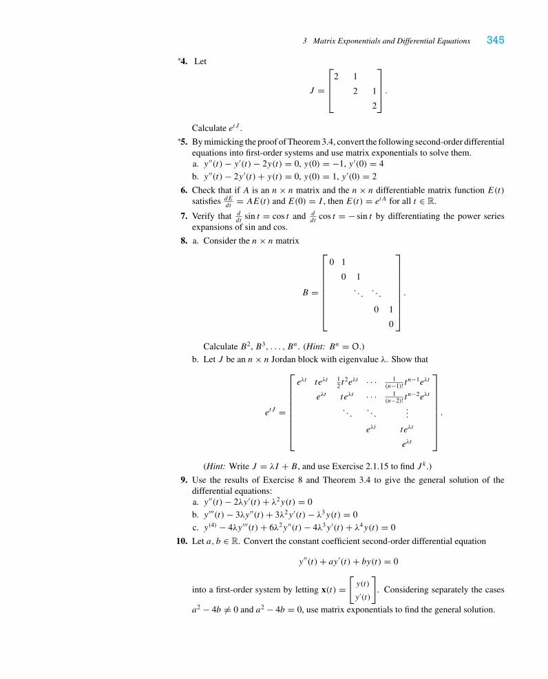
3 Matrix Exponentials and Differential Equations 345
4.∗ Let
J =
⎡⎢⎢⎣
2 1
2 1
2
⎤⎥⎥⎦ .
Calculate etJ .
5.∗ By mimicking the proof of Theorem 3.4, convert the following second-order differentialequations into first-order systems and use matrix exponentials to solve them.a. y ′′(t)− y ′(t)− 2y(t) = 0, y(0) = −1, y ′(0) = 4
b. y ′′(t)− 2y ′(t)+ y(t) = 0, y(0) = 1, y ′(0) = 2
6. Check that if A is an n× n matrix and the n× n differentiable matrix function E(t)satisfies dE
dt= AE(t) and E(0) = I , then E(t) = etA for all t ∈ R.
7. Verify that ddt
sin t = cos t and ddt
cos t = − sin t by differentiating the power seriesexpansions of sin and cos.
8. a. Consider the n× n matrix
B =
⎡⎢⎢⎢⎢⎢⎢⎢⎢⎣
0 1
0 1. . .
. . .
0 1
0
⎤⎥⎥⎥⎥⎥⎥⎥⎥⎦.
Calculate B2, B3, . . . , Bn. (Hint: Bn = O.)
b. Let J be an n× n Jordan block with eigenvalue λ. Show that
etJ =
⎡⎢⎢⎢⎢⎢⎢⎢⎢⎣
eλt teλt 12 t
2eλt · · · 1(n−1)! t
n−1eλt
eλt teλt · · · 1(n−2)! t
n−2eλt
. . .. . .
...
eλt teλt
eλt
⎤⎥⎥⎥⎥⎥⎥⎥⎥⎦.
(Hint: Write J = λI + B, and use Exercise 2.1.15 to find J k .)
9. Use the results of Exercise 8 and Theorem 3.4 to give the general solution of thedifferential equations:a. y ′′(t)− 2λy ′(t)+ λ2y(t) = 0
b. y ′′′(t)− 3λy ′′(t)+ 3λ2y ′(t)− λ3y(t) = 0
c. y(4) − 4λy ′′′(t)+ 6λ2y ′′(t)− 4λ3y ′(t)+ λ4y(t) = 0
10. Let a, b ∈ R. Convert the constant coefficient second-order differential equation
y ′′(t)+ ay ′(t)+ by(t) = 0
into a first-order system by letting x(t) =[y(t)
y ′(t)
]. Considering separately the cases
a2 − 4b �= 0 and a2 − 4b = 0, use matrix exponentials to find the general solution.
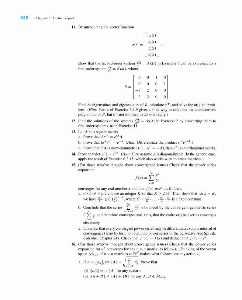
346 Chapter 7 Further Topics
11. By introducing the vector function
z(t) =
⎡⎢⎢⎢⎢⎣
x1(t)
x2(t)
x ′1(t)
x ′2(t)
⎤⎥⎥⎥⎥⎦,
show that the second-order system d2xdt2
= Ax(t) in Example 8 can be expressed as afirst-order system dz
dt= Bz(t), where
B =
⎡⎢⎢⎢⎢⎣
0 0 1 0
0 0 0 1
−3 2 0 0
2 −3 0 0
⎤⎥⎥⎥⎥⎦.
Find the eigenvalues and eigenvectors of B, calculate etB , and solve the original prob-lem. (Hint: Part c of Exercise 5.1.9 gives a slick way to calculate the characteristicpolynomial of B, but it’s not too hard to do so directly.)
12. Find the solutions of the systems d2xdt2
= Ax(t) in Exercise 2 by converting them tofirst-order systems, as in Exercise 11.
13. Let A be a square matrix.a. Prove that AetA = etAA.
b. Prove that (eA)−1 = e−A. (Hint: Differentiate the product etAe−tA.)
c. Prove that ifA is skew-symmetric (i.e.,AT = −A), then eA is an orthogonal matrix.
14. Prove that det(eA) = etrA. (Hint: First assumeA is diagonalizable. In the general case,apply the result of Exercise 6.2.15, which also works with complex matrices.)
15. (For those who’ve thought about convergence issues) Check that the power seriesexpansion
f (x) =∞∑k=0
xk
k!converges for any real number x and that f (x) = ex , as follows.a. Fix x �= 0 and choose an integer K so that K ≥ 2|x|. Then show that for k > K ,
we have |x|kk! ≤ C ( 1
2
)k−K, where C = |x|
K· . . . · |x|
2 · |x|1 is a fixed constant.
b. Conclude that the series∞∑
k=K+1
|x|kk! is bounded by the convergent geometric series
C∞∑j=1
12j and therefore converges and, thus, that the entire original series converges
absolutely.
c. It is a fact that every convergent power series may be differentiated (on its interval ofconvergence) term by term to obtain the power series of the derivative (see Spivak,Calculus, Chapter 24). Check that f ′(x) = f (x) and deduce that f (x) = ex .
16. (For those who’ve thought about convergence issues) Check that the power seriesexpansion for eA converges for any n× n matrix, as follows. (Thinking of the vectorspace Mn×n of n× n matrices as Rn
2makes what follows less mysterious.)
a. If A = [aij], set ‖A‖ =
√n∑
i,j=1a2ij . Prove that
(i) ‖cA‖ = |c|‖A‖ for any scalar c
(ii) ‖A+ B‖ ≤ ‖A‖ + ‖B‖ for any A,B ∈ Mn×n
Historical Notes 347
(iii) ‖AB‖ ≤ ‖A‖‖B‖ for any A,B ∈ Mn×n. (Hint: Express the entries of thematrix product in terms of the row vectors Ai and the column vectors bj .) Inparticular, deduce that ‖Ak‖ ≤ ‖A‖k for all positive integers k.
b. It is a fact from analysis that if vk ∈ RN is a sequence of vectors in RN with the
property that∞∑k=1
‖vk‖ converges (in R), then∞∑k=1
vk converges (in RN ). Using this
fact, prove that∞∑k=0
Ak
k! converges for any matrix A ∈ Mn×n.
c. (For those who know what a Cauchy sequence is) Prove the fact stated in part b.
HISTORICAL NOTESThe Jordan of the Jordan canonical form is not Wilhelm Jordan, mentioned in earlier his-torical notes, but Camille Jordan (1838–1922), a brilliant French mathematician. Jordanwas interested in algebra and its application to geometry. In particular, he studied algebraicobjects called groups, which are used to study symmetry—in Jordan’s case, the structure ofcrystals. In 1870, Jordan published his most important work, a summary of group theoryand related algebraic notions, in which he introduced the “canonical form” for matrices oftransformations that now bears his name. At the time, mathematicians were very active inmany countries. Given the lack of modern communication methods, it was not uncommonfor someone to “discover” a result that had already been discovered. The history is fuzzy,but a number of different people, including Karl Weierstrass (1815–1897), Henry Smith(1826–1883), and Hermann Grassmann (1809–1877), might also be given credit. Ferdi-nand Frobenius (1849–1917), publishing after Jordan, explained the Jordan canonical formin its most general terms.
In this chapter you also encountered a contemporary application of linear algebra toprojection on a computer screen or, more generally speaking, to the concept of perspective.Questions about perspective date back to the ancient Greeks. Euclid (ca. 325–265 BCE), inone of his many lasting works, Optics, raised numerous questions on perspective, wonderinghow simple geometric objects such as a circle appear when viewed from different planes.
Later discourses on perspective can be found during the fifteenth and sixteenth cen-turies, but not from mathematicians. The painter Leonardo Da Vinci (1452–1519) thoughtof painting as a projection of the three-dimensional world onto a two-dimensional world andsought the best way to perform this “mapping.” The Italian architect Fillipo Brunelleschi(1377–1446) formulated perspective in a mathematical way and defined the concept of the“vanishing point,” that place where parallel lines meet in one’s view. It was the Germanscientist and astronomer Johannes Kepler (1571–1630) who adopted the interpretation thatthere was a point at infinity through which lines could be drawn.
Kepler’s idea paved the way for a mathematical point of view of perspective andprojection, leading to the field called projective geometry. His work led to study by GirardDesargues (1591–1661), René Descartes (1597–1650), and Étienne Pascal (1588–1651)and his son, Blaise (1623–1662). The field then lay dormant until the early nineteenthcentury, at which time Jean-Victor Poncelet (1788–1867) did seminal work on projectiveduality.

This page intentionally left blank

349
FOR FURTHER READING
More on Linear AlgebraBretscher, Otto, Linear Algebra with Applications, Third Edition, Prentice Hall, 2004. A
bit more depth on dynamical systems, discrete and continuous.Friedberg, Stephen H., Insel, Arnold J., and Spence, Lawrence E., Linear Algebra, Fourth
Edition, Prentice Hall, 2002. A well-written, somewhat more advanced book concen-trating on the theoretical aspects.
Lawson, Terry, Linear Algebra, John Wiley & Sons, 1996. A book comparable in level to,but slightly more difficult than, this text. More details on complex vector spaces anddiscussion of the geometry of orthogonal matrices.
Sadun, Lorenzo, Applied Linear Algebra: The Decoupling Principle, Second Edition,American Mathematical Society, 2008. This book, along with Strang’s Introductionto Applied Mathematics, delves deeply into Fourier series and differential equations,including a fair amount of infinite-dimensional linear algebra.
Strang, Gilbert, Introduction to Linear Algebra, Fourth Edition, Wellesley-CambridgePress, 2009. A book more elementary than this, with more emphasis on numericalapplications and less on definitions and proofs.
———, Linear Algebra and Its Applications, Fourth Edition, Saunders, 2008. The classic,with far more depth on applications, and the inspiration for our brief section on graphtheory.
Wilkinson, J. M., The Algebraic Eigenvalue Problem, Oxford Science Publications, 1988.An advanced book that includes a proof of the algorithm based on iterating the QRdecomposition to calculate eigenvalues and eigenvectors numerically.
Historical MattersAlthoen, Steven C. , and McLaughlin, Renate, “Gauss-Jordan Reduction: A Brief History,”
American Mathematical Monthly, 94, No. 2. (February 1987), pp. 130–142.Cooke, Roger, The History of Mathematics: A Brief Course, Second Edition, John Wiley
& Sons, 2005.Kline, Morris, Mathematical Thought from Ancient to Modern Times, Oxford University
Press, 1972.Mac Tutor History of Mathemathics Archive. University of St. Andrews, Scotland. http://
www-history.mcs.st-and.ac.uk/. An informative, searchable, and amazingly compre-hensive resource.
Maor, Eli, e: The Story of a Number, Princeton University Press, 1994.
Other Interesting SourcesArtin, Michael, Algebra, Prentice Hall, 1991. A sophisticated abstract algebra text that
incorporates linear algebraic and geometric material throughout.Hill, F. S. Jr., and Stephen M. Kelly, Computer Graphics, Macmillan, 2006. See especially
Chapters 10–12 for three-dimensional graphics.

350 For Further Reading
Foley, James D., Andries van Dam, Stephen K. Feiner, and John F. Hughes, ComputerGraphics: Principles and Practice, Second Edition, Addison-Wesley, 1995. One ofthe respected texts used by computer scientists.
Golubitsky, Martin, and Michael Dellnitz, Linear Algebra and Differential Equations UsingMATLAB, Brooks/Cole, 1999. An integrated treatment of linear algebra and differen-tial equations, with interesting differential equations material on planar and higher-dimensional systems and bifurcation theory.
Pedoe, Dan, Geometry: A Comprehensive Course, Dover Publications, 1988 (originallypublished by Cambridge University Press, 1970). A fabulous, linear-algebraic treat-ment of geometry, both Euclidean and non-Euclidean, with an excellent treatment ofprojective geometry and quadrics.
Shifrin, Theodore, Abstract Algebra: A Geometric Approach, Prentice Hall, 1996. A firstcourse in abstract algebra that will be accessible to anyone who has enjoyed this linearalgebra course.
———, Multivariable Mathematics: Linear Algebra, Multivariable Calculus, and Man-ifolds, John Wiley & Sons, 2004. An integrated treatment of the linear algebra inthis course and rigorous multivariable calculus. The derivative as the linearization isapparent throughout; a detailed treatment of determinants and n-dimensional volumeand the change-of-variables theorem.
Spivak, Michael, Calculus, Fourth Edition, Publish or Perish, 2008. The ultimate sourcefor calculus “done right.”
Strang, Gilbert, Introduction to Applied Mathematics, Wellesley-Cambridge Press, 1986.Although not a great source for the details and proofs, this book is a wonderful expo-sition of modern applied mathematics, in which the author emphasizes how even thedifferential equations problems follow the models established by linear algebra.
351
ANSWERS TO SELECTED EXERCISES
1.1.3 (4, 3, 7), (0, 5,−1), (2,−1, 3)
1.1.5 a., b. yes; c. no
1.1.6 b. x = (−1, 2)+ t (3, 1); f. x = (1, 2, 1)+ t (1,−1,−1) ; h. x = (1, 1, 0,−1)+t (1,−2, 3,−1)
1.1.8 a. no; b., c. yes
1.1.9 a., c. yes; b., d. no
1.1.10 b. x = (1, 1, 1)+ s(−3, 0, 1)+ t (1, 3, 1)1.1.12 The planes P1 and P4 are the same. Note that (0, 2, 1) = (1, 1, 0)+ 1(1, 0, 1)+
1(−2, 1, 0); both vectors (1,−1,−1) and (3,−1, 1) are in the plane spanned by(1, 0, 1) and (−2, 1, 0). Thus, every point of P4 lies in the plane P1. On theother hand, (1, 1, 0) = (0, 2, 1)+ 1(1,−1,−1)+ 0(3,−1, 1), and both vectors(1, 0, 1) and (−2, 1, 0) are in the plane spanned by (1,−1,−1) and (3,−1, 1).So every point of P1 lies in the plane P4. This means that P1 = P4. Similarly,P2 = P3.
1.1.15 The battle plan is to let−→AB = x and
−→AC = y and then to express
−→AE and−→
AQ as linear combinations of x and y. We are given the facts that−→AD = 2
3 x
and−→CE = 2
5
−→CB = 2
5 (x − y). Therefore,−→AE = −→
AC + −→CE = y + 2
5 (x − y) =25 x + 3
5 y = 15 (2x + 3y). On the other hand, becauseQ is the midpoint of CD, we
have−→AQ = −→
AC + 12
−→CD = y + 1
2
(23 x − y
) = 12 y + 1
3 x = 16 (2x + 3y). Compar-
ing the final expressions for−→AE and
−→AQ, we see that
−→AQ = 5
6
−→AE, so c = 5/6.
1.1.23 Suppose that � and P intersect; then there must be a point, x, contained in both. Thismeans that there are real numbers r , s, and t satisfying x = x0 + rv = su + tv.Then x0 = su + tv − rv = su + (t − r)v, so x0 ∈ Span (u, v), whence x0 ∈ P.
1.2.1 c. −25, θ = arccos(−5/13); f. 2, θ = arccos(1/5)
1.2.2 c. − 513 (7,−4), − 5
13 (1, 8); f. (−1, 0, 1), 125 (3,−4, 5)
1.2.4 arccos√
2/3 ≈ 0.62 radians ≈ 35.3◦
1.2.6 Since θ = arccos(−1/6), we have x · y = ‖x‖‖y‖ cos θ = −1.Then (x + 2y) · (x − y) = ‖x‖2 − x · y + 2(y · x)− 2‖y‖2 = 9 + 1 − 2 − 8 =0, so (x + 2y) and (x − y) are orthogonal, by definition.
1.2.10 π/6
1.2.14 Let x = −→CA and y = −→
CB. Then−→AB = y − x, and
‖−→AB‖2 = ‖y − x‖2 = ‖y‖2 − 2y · x + ‖x‖2 = a2 − 2ab cos θ + b2 .
1.3.1 b. x1 − x2 + x3 = 1; d. x1 − 2x2 + x3 = 1; f. x1 + x2 + x3 + x4 = 0
1.3.2 a., d. x1 + 2x2 − x3 = 3; b., c. x1 + 2x2 − x3 = 2
1.3.3 c. x = (5, 0, 0, 0)+ x2(−1, 1, 0, 0)+ x3(1, 0, 1, 0)+ x4(−2, 0, 0, 1); d. x =(4, 0, 0, 0)+ x2(2, 1, 0, 0)+ x3(−3, 0, 1, 0)+ x4(0, 0, 0, 1)
352 Answers to Selected Exercises
1.3.4 c. 1/√
3; e. 2/9
1.3.6 a. x = x2(−5, 1, 0)+ x3(2, 0, 1); b. (3, 0, 0), x = (3, 0, 0)+ x2(−5, 1, 0)+x3(2, 0, 1); c. x = x2(−5, 1, 0, 0)+ x3(2, 0, 1, 0)+ x4(−1, 0, 0, 1),x = (3, 0, 0, 0)+ x2(−5, 1, 0, 0)+ x3(2, 0, 1, 0)+ x4(−1, 0, 0, 1)
1.3.7 a. a = (2,−3). b. |c|/‖a‖ = 5/√
13. Remember that this comes from choosinga point x0 on the line, say x0 = (1,−1), and projecting the vector x0 onto thenormal vector a. c. The line through 0 with direction vector a has parametricequation x = t (2,−3). This line intersects the given line when 2(2t)− 3(−3t) =5, i.e., when t = 5/13. Thus, p = 5
13 (2,−3) is the point on the line closest to theorigin. ‖p‖ = 5/
√13 checks with our answer to part b. d. We choose a point
x0 = (1,−1) on the line and find the length of the projection of x0 − w onto thenormal vector a: ‖proja(x0 − w)‖ = |a · (x0 − w)|/‖a‖ = 2/
√13. e. The line
through w with direction vector a has parametric equation x = (3, 1)+ t (2,−3).This line intersects the given line when 2(3 + 2t)− 3(1 − 3t) = 5, i.e., whent = 2/13. This gives the point q = w + 2
13 a on the line. The distance is therefore‖q − w‖ = ‖ 2
13 a‖ = 2√13
.
1.3.10 a. ax1 + bx2 = 0 (a and b arbitrary real numbers, not both 0)
1.4.1 b. x = (−2, 0, 1)+ x2(−2, 1, 0)
1.4.2 b., c., d., f., g. are in echelon form; c. and g. are in reduced echelon form.
1.4.3 a.
⎡⎢⎣
1 0 −1
0 1 −1
0 0 0
⎤⎥⎦, x = x3
⎡⎢⎣
1
1
1
⎤⎥⎦; e.
[1 −2 0 1
0 0 1 −1
],
x = x2
⎡⎢⎢⎢⎣
2
1
0
0
⎤⎥⎥⎥⎦+ x4
⎡⎢⎢⎢⎣
−1
0
1
1
⎤⎥⎥⎥⎦; g.
⎡⎢⎢⎢⎣
1 0 2 0 2
0 1 1 0 1
0 0 0 1 −1
0 0 0 0 0
⎤⎥⎥⎥⎦,
x = x3
⎡⎢⎢⎢⎢⎢⎢⎣
−2
−1
1
0
0
⎤⎥⎥⎥⎥⎥⎥⎦
+ x5
⎡⎢⎢⎢⎢⎢⎢⎣
−2
−1
0
1
1
⎤⎥⎥⎥⎥⎥⎥⎦
1.4.4 a. x =⎡⎢⎣
2
−1
0
⎤⎥⎦+ x3
⎡⎢⎣
1
−1
1
⎤⎥⎦; c. inconsistent
1.4.5 b. x = x2(0, 1, 0)+ x3(1, 0, 1)
1.4.8 x = (1/√
2, 1/√
2, 0)
1.4.10 a. (1,−1,−1, 1)
1.4.11 a. x = s(−1, 1, 1, 0)+ t (−1,−2, 0, 1)
1.4.13 Use Proposition 2.1. For each i = 1, . . . , m, we have Ai · (cx) = c(Ai · x) andAi · (x + y) = Ai · x + Ai · y.
1.5.1 b = v1 − v2 + v3
1.5.2 b. yes; a., c. no
1.5.3 b. 2b1 + b2 − b3 = 0; d. None.
Answers to Selected Exercises 353
1.5.7 b. A =[
0 1 0 1
0 0 1 1
]; d. A =
[1 −1 1
1 −1 1
].
1.5.8 a. 0, 3; b. for α = 0, b must satisfy b2 = 0; for α = 3, b must satisfy b2 = 3b1.
1.5.12 a. none, as Ax = 0 is always consistent; b. take r = m = n; e. take r < m andr < n
1.5.14 a. Afurther hint: By repeatedly doing row operation (iii), we can obtain a row of 0’sin the matrix, so the echelon form must have a row of 0’s. An alternative approach isthis: Because the sum of the rows is 0, any vector b for whichAx = b is consistentmust satisfy b1 + · · · + bm = 0. (To see this, note that if Ax = b, then this meansthat Aix = bi , so 0 = (A1 + · · · + Am)x = A1x + · · · + Amx = b1 + · · · + bm.)Thus, by Proposition 5.1, we must have rank(A) < m.
1.6.1 64%, 32
1.6.5 y = 3x2 − 5x + 1
1.6.9 center (−1, 2), radius 5
1.6.12 a. (a, b, c, d, e) = (3, 6, 5, 1, 3)
1.6.13 a. (A,B,C,D) = 12 (1, 1, 3, 3)
1.6.14 a. I1 = 3 amps; b. I3 = 3 amps; c. I3 = V(
1R1
+ 1R2
)
1.6.16 b. No matter what the original cat and mouse populations are, the cats proliferateand the mice die out.
2.1.1 b.
[0 3
2 5
]; f.
[5 8
13 20
]; g.
[1 4 5
3 10 11
]; h. not defined; k.
[4 4
5 6
];
l.
⎡⎢⎣
0 1 2
1 2 1
2 7 8
⎤⎥⎦
2.1.5 a. As a hint, see part a of Exercise 1.2.16.
2.1.7 b. Either A =[
0 β
0 0
]or
[0 0
β 0
]for some real number β or A =
α
[1 β
−1/β −1
], α any real number, β �= 0.
2.2.3 a. Since T
([1
0
])=[
2
−3
], that is the first column of A. For the second col-
umn, we need T
([0
1
])= T
([2
1
]− 2
[1
0
])= T
([2
1
])− T
(2
[1
0
])=
T
([2
1
])− 2T
([1
0
])=[
−1
1
]− 2
[2
−3
]=[
−5
7
], and this is the second
column of A. Thus, A =[
2 −5
−3 7
].
2.2.4 b., c., e. yes; a., d., f. no
2.2.5 b. A =[
12
12
12
12
]; e. A =
[− 2
5 − 45
15
25
]
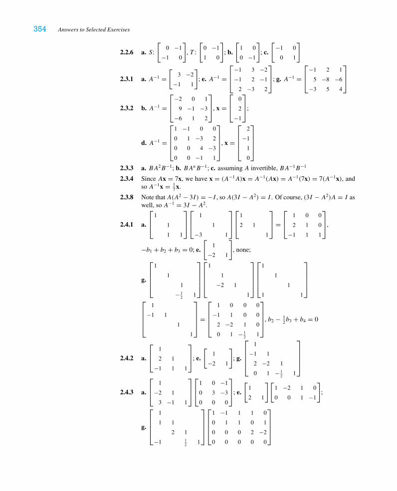
354 Answers to Selected Exercises
2.2.6 a. S:
[0 −1
−1 0
], T :
[0 −1
1 0
]; b.
[1 0
0 −1
]; c.
[−1 0
0 1
]
2.3.1 a. A−1 =[
3 −2
−1 1
]; e. A−1 =
⎡⎢⎣
−1 3 −2
−1 2 −1
2 −3 2
⎤⎥⎦; g. A−1 =
⎡⎢⎣
−1 2 1
5 −8 −6
−3 5 4
⎤⎥⎦
2.3.2 b. A−1 =⎡⎢⎣
−2 0 1
9 −1 −3
−6 1 2
⎤⎥⎦, x =
⎡⎢⎣
0
2
−1
⎤⎥⎦;
d. A−1 =
⎡⎢⎢⎢⎣
1 −1 0 0
0 1 −3 2
0 0 4 −3
0 0 −1 1
⎤⎥⎥⎥⎦, x =
⎡⎢⎢⎢⎣
2
−1
1
0
⎤⎥⎥⎥⎦
2.3.3 a. BA2B−1; b. BAnB−1; c. assuming A invertible, BA−1B−1
2.3.4 Since Ax = 7x, we have x = (A−1A)x = A−1(Ax) = A−1(7x) = 7(A−1x), andso A−1x = 1
7 x.
2.3.8 Note thatA(A2 − 3I ) = −I , soA(3I − A2) = I . Of course, (3I − A2)A = I aswell, so A−1 = 3I − A2.
2.4.1 a.
⎡⎢⎣
1
1
1 1
⎤⎥⎦
⎡⎢⎣
1
1
−3 1
⎤⎥⎦
⎡⎢⎣
1
2 1
1
⎤⎥⎦ =
⎡⎢⎣
1 0 0
2 1 0
−1 1 1
⎤⎥⎦,
−b1 + b2 + b3 = 0; e.
[1
−2 1
], none;
g.
⎡⎢⎢⎢⎣
1
1
1
− 12 1
⎤⎥⎥⎥⎦
⎡⎢⎢⎢⎣
1
1
−2 1
1
⎤⎥⎥⎥⎦
⎡⎢⎢⎢⎣
1
1
1
1 1
⎤⎥⎥⎥⎦
⎡⎢⎢⎢⎣
1
−1 1
1
1
⎤⎥⎥⎥⎦ =
⎡⎢⎢⎢⎣
1 0 0 0
−1 1 0 0
2 −2 1 0
0 1 − 12 1
⎤⎥⎥⎥⎦, b2 − 1
2b3 + b4 = 0
2.4.2 a.
⎡⎢⎣
1
2 1
−1 1 1
⎤⎥⎦; e.
[1
−2 1
]; g.
⎡⎢⎢⎢⎣
1
−1 1
2 −2 1
0 1 − 12 1
⎤⎥⎥⎥⎦
2.4.3 a.
⎡⎢⎣
1
−2 1
3 −1 1
⎤⎥⎦
⎡⎢⎣
1 0 −1
0 3 −3
0 0 0
⎤⎥⎦; e.
[1
2 1
][1 −2 1 0
0 0 1 −1
];
g.
⎡⎢⎢⎢⎣
1
1 1
2 1
−1 12 1
⎤⎥⎥⎥⎦
⎡⎢⎢⎢⎣
1 −1 1 1 0
0 1 1 0 1
0 0 0 2 −2
0 0 0 0 0
⎤⎥⎥⎥⎦
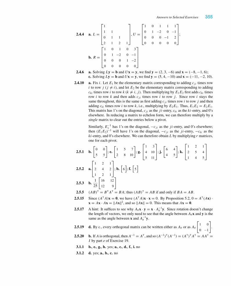
Answers to Selected Exercises 355
2.4.4 a. L =
⎡⎢⎢⎢⎣
1
1 1
0 1 1
2 1 2 1
⎤⎥⎥⎥⎦, U =
⎡⎢⎢⎢⎣
1 0 1 1 1
0 1 −2 0 −1
0 0 0 −1 2
0 0 0 0 0
⎤⎥⎥⎥⎦;
b. R =
⎡⎢⎢⎢⎣
1 0 1 0 3
0 1 −2 0 −1
0 0 0 1 −2
0 0 0 0 0
⎤⎥⎥⎥⎦
2.4.6 a. Solving Ly = b and Ux = y, we find y = (2, 3,−6) and x = (−8,−1, 6);c. Solving Ly = b and Ux = y, we find y = (5, 4,−10) and x = (−11,−2, 10).
2.4.10 a. Fix i. Let E1 be the elementary matrix corresponding to adding cji times rowi to row j (j �= i), and let E2 be the elementary matrix corresponding to addingcki times row i to row k (k �= i, j ). Then multiplying by E1E2 first adds cki timesrow i to row k and then adds cji times row i to row j . Since row i stays thesame throughout, this is the same as first adding cji times row i to row j and thenadding cki times row i to row k, i.e., multiplying by E2E1. Thus, E1E2 = E2E1.This matrix has 1’s on the diagonal, cji as the ji-entry, cki as the ki-entry, and 0’selsewhere. In reducing a matrix to echelon form, we can therefore multiply by asingle matrix to clear out the entries below a pivot.
Similarly, E−11 has 1’s on the diagonal, −cji as the ji-entry, and 0’s elsewhere;
then (E1E2)−1 will have 1’s on the diagonal, −cji as the ji-entry, −cki as the
ki-entry, and 0’s elsewhere. We can therefore obtain L by multiplying r matrices,one for each pivot.
2.5.1 b.
[0 0
5 5
]; e.
[1 5 7
2 8 10
]; g.
⎡⎢⎣
1 3
4 10
5 11
⎤⎥⎦; j.
[6 4
4 5
]; k.
⎡⎢⎣
1 2 1
2 5 4
1 4 5
⎤⎥⎦
2.5.2 a.
⎡⎢⎣
1 2 1
2 4 2
1 2 1
⎤⎥⎦; b.
[6]; f.[
5]
2.5.3 b.1
25
[16 12
12 9
]
2.5.5 (AB)T = BTAT = BA; thus (AB)T = AB if and only if BA = AB.
2.5.15 Since (ATA)x = 0, we have (ATA)x · x = 0. By Proposition 5.2, 0 = AT(Ax) ·x = Ax · Ax = ‖Ax‖2, and so ‖Ax‖ = 0. This means that Ax = 0.
2.5.17 A hint: It suffices to see why Aθx · y = x · A−1θ y. Since rotation doesn’t change
the length of vectors, we only need to see that the angle between Aθx and y is thesame as the angle between x and A−1
θ y.
2.5.19 d. By c., every orthogonal matrix can be written either as Aθ or as Aθ
[1 0
0 −1
].
2.5.20 b. IfA is orthogonal, thenA−1 = AT, and so (A−1)T(A−1) = (AT)TAT = AAT =I by part e of Exercise 19.
3.1.1 b., e., g., h. yes; a., c., d., f., i. no
3.1.2 d. yes; a., b., c. no
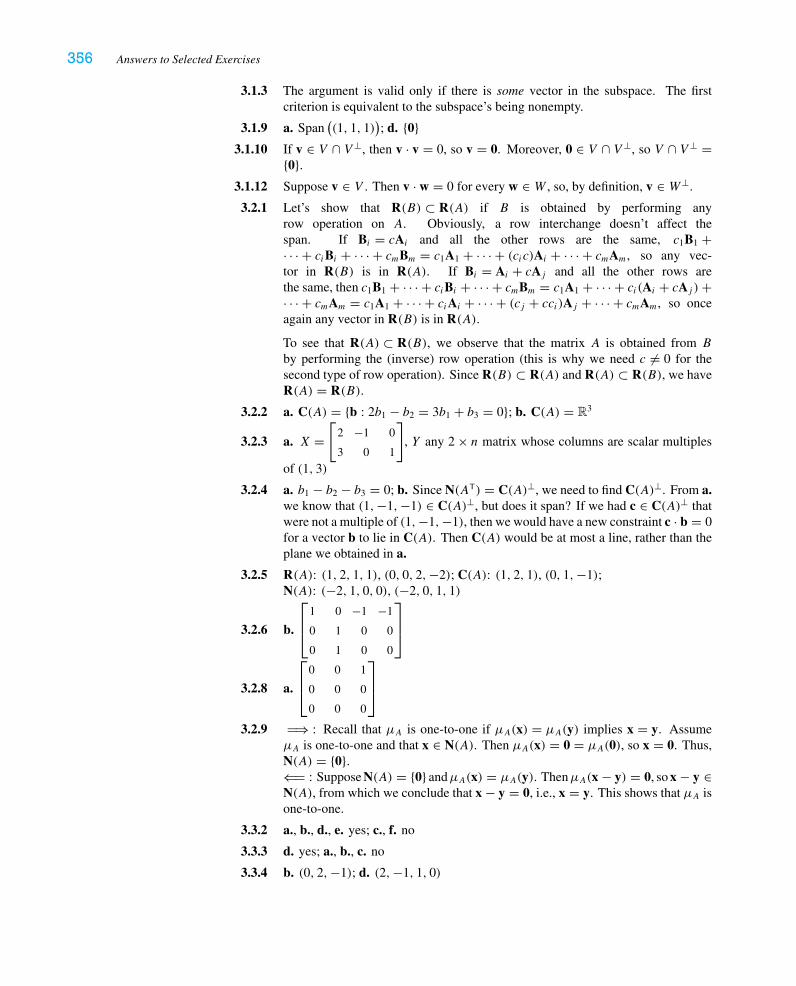
356 Answers to Selected Exercises
3.1.3 The argument is valid only if there is some vector in the subspace. The firstcriterion is equivalent to the subspace’s being nonempty.
3.1.9 a. Span((1, 1, 1)
); d. {0}
3.1.10 If v ∈ V ∩ V ⊥, then v · v = 0, so v = 0. Moreover, 0 ∈ V ∩ V ⊥, so V ∩ V ⊥ ={0}.
3.1.12 Suppose v ∈ V . Then v · w = 0 for every w ∈ W , so, by definition, v ∈ W⊥.
3.2.1 Let’s show that R(B) ⊂ R(A) if B is obtained by performing anyrow operation on A. Obviously, a row interchange doesn’t affect thespan. If Bi = cAi and all the other rows are the same, c1B1 +· · · + ciBi + · · · + cmBm = c1A1 + · · · + (cic)Ai + · · · + cmAm, so any vec-tor in R(B) is in R(A). If Bi = Ai + cAj and all the other rows arethe same, then c1B1 + · · · + ciBi + · · · + cmBm = c1A1 + · · · + ci(Ai + cAj )+· · · + cmAm = c1A1 + · · · + ciAi + · · · + (cj + cci)Aj + · · · + cmAm, so onceagain any vector in R(B) is in R(A).
To see that R(A) ⊂ R(B), we observe that the matrix A is obtained from B
by performing the (inverse) row operation (this is why we need c �= 0 for thesecond type of row operation). Since R(B) ⊂ R(A) and R(A) ⊂ R(B), we haveR(A) = R(B).
3.2.2 a. C(A) = {b : 2b1 − b2 = 3b1 + b3 = 0}; b. C(A) = R3
3.2.3 a. X =[
2 −1 0
3 0 1
], Y any 2 × n matrix whose columns are scalar multiples
of (1, 3)
3.2.4 a. b1 − b2 − b3 = 0; b. Since N(AT) = C(A)⊥, we need to find C(A)⊥. From a.we know that (1,−1,−1) ∈ C(A)⊥, but does it span? If we had c ∈ C(A)⊥ thatwere not a multiple of (1,−1,−1), then we would have a new constraint c · b = 0for a vector b to lie in C(A). Then C(A) would be at most a line, rather than theplane we obtained in a.
3.2.5 R(A): (1, 2, 1, 1), (0, 0, 2,−2); C(A): (1, 2, 1), (0, 1,−1);N(A): (−2, 1, 0, 0), (−2, 0, 1, 1)
3.2.6 b.
⎡⎢⎣
1 0 −1 −1
0 1 0 0
0 1 0 0
⎤⎥⎦
3.2.8 a.
⎡⎢⎣
0 0 1
0 0 0
0 0 0
⎤⎥⎦
3.2.9 �⇒ : Recall that μA is one-to-one if μA(x) = μA(y) implies x = y. AssumeμA is one-to-one and that x ∈ N(A). Then μA(x) = 0 = μA(0), so x = 0. Thus,N(A) = {0}.⇐� : Suppose N(A) = {0} andμA(x) = μA(y). ThenμA(x − y) = 0, so x − y ∈N(A), from which we conclude that x − y = 0, i.e., x = y. This shows that μA isone-to-one.
3.3.2 a., b., d., e. yes; c., f. no
3.3.3 d. yes; a., b., c. no
3.3.4 b. (0, 2,−1); d. (2,−1, 1, 0)
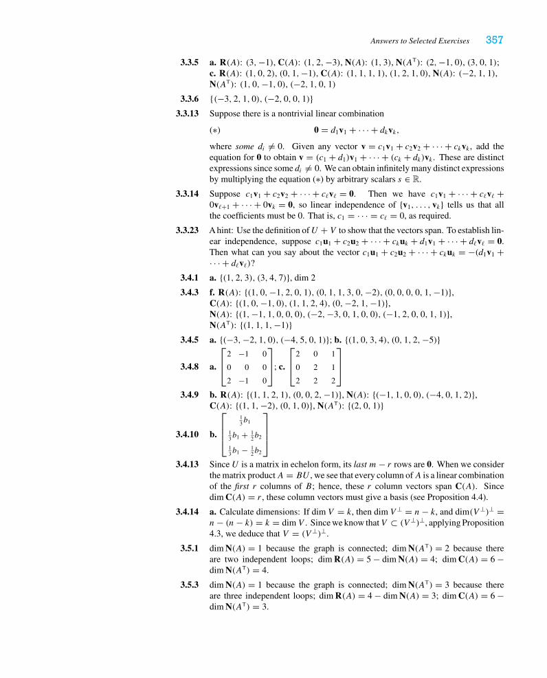
Answers to Selected Exercises 357
3.3.5 a. R(A): (3,−1), C(A): (1, 2,−3), N(A): (1, 3), N(AT): (2,−1, 0), (3, 0, 1);c. R(A): (1, 0, 2), (0, 1,−1), C(A): (1, 1, 1, 1), (1, 2, 1, 0), N(A): (−2, 1, 1),N(AT): (1, 0,−1, 0), (−2, 1, 0, 1)
3.3.6 {(−3, 2, 1, 0), (−2, 0, 0, 1)}3.3.13 Suppose there is a nontrivial linear combination
(∗) 0 = d1v1 + · · · + dkvk,where some di �= 0. Given any vector v = c1v1 + c2v2 + · · · + ckvk , add theequation for 0 to obtain v = (c1 + d1)v1 + · · · + (ck + dk)vk . These are distinctexpressions since some di �= 0. We can obtain infinitely many distinct expressionsby multiplying the equation (∗) by arbitrary scalars s ∈ R.
3.3.14 Suppose c1v1 + c2v2 + · · · + c�v� = 0. Then we have c1v1 + · · · + c�v� +0v�+1 + · · · + 0vk = 0, so linear independence of {v1, . . . , vk} tells us that allthe coefficients must be 0. That is, c1 = · · · = c� = 0, as required.
3.3.23 A hint: Use the definition ofU + V to show that the vectors span. To establish lin-ear independence, suppose c1u1 + c2u2 + · · · + ckuk + d1v1 + · · · + d�v� = 0.Then what can you say about the vector c1u1 + c2u2 + · · · + ckuk = −(d1v1 +· · · + d�v�)?
3.4.1 a. {(1, 2, 3), (3, 4, 7)}, dim 2
3.4.3 f. R(A): {(1, 0,−1, 2, 0, 1), (0, 1, 1, 3, 0,−2), (0, 0, 0, 0, 1,−1)},C(A): {(1, 0,−1, 0), (1, 1, 2, 4), (0,−2, 1,−1)},N(A): {(1,−1, 1, 0, 0, 0), (−2,−3, 0, 1, 0, 0), (−1, 2, 0, 0, 1, 1)},N(AT): {(1, 1, 1,−1)}
3.4.5 a. {(−3,−2, 1, 0), (−4, 5, 0, 1)}; b. {(1, 0, 3, 4), (0, 1, 2,−5)}
3.4.8 a.
⎡⎢⎣
2 −1 0
0 0 0
2 −1 0
⎤⎥⎦; c.
⎡⎢⎣
2 0 1
0 2 1
2 2 2
⎤⎥⎦
3.4.9 b. R(A): {(1, 1, 2, 1), (0, 0, 2,−1)}, N(A): {(−1, 1, 0, 0), (−4, 0, 1, 2)},C(A): {(1, 1,−2), (0, 1, 0)}, N(AT): {(2, 0, 1)}
3.4.10 b.
⎡⎢⎢⎣
13b1
13b1 + 1
2b2
13b1 − 1
2b2
⎤⎥⎥⎦
3.4.13 Since U is a matrix in echelon form, its last m− r rows are 0. When we considerthe matrix productA = BU , we see that every column ofA is a linear combinationof the first r columns of B; hence, these r column vectors span C(A). Sincedim C(A) = r , these column vectors must give a basis (see Proposition 4.4).
3.4.14 a. Calculate dimensions: If dim V = k, then dim V ⊥ = n− k, and dim(V ⊥)⊥ =n− (n− k) = k = dim V . Since we know thatV ⊂ (V ⊥)⊥, applying Proposition4.3, we deduce that V = (V ⊥)⊥.
3.5.1 dim N(A) = 1 because the graph is connected; dim N(AT) = 2 because thereare two independent loops; dim R(A) = 5 − dim N(A) = 4; dim C(A) = 6 −dim N(AT) = 4.
3.5.3 dim N(A) = 1 because the graph is connected; dim N(AT) = 3 because thereare three independent loops; dim R(A) = 4 − dim N(A) = 3; dim C(A) = 6 −dim N(AT) = 3.
358 Answers to Selected Exercises
3.6.2 a., c., e. yes; b., d., f. no
3.6.3 a., f., g. yes; b., c., d., e. no
3.6.4 mn
3.6.5 dim U = dim L = 12n(n+ 1), dim D = n
3.6.6 a. not a subspace since 0 does not have this property; c. a one-dimensionalsubspace with basis {e−2t }; f. a two-dimensional subspace with basis {cos t, sin t}:show that if f lies in this subspace and has the properties f (0) = a and f ′(0) =b, then f (t) = a cos t + b sin t (Hint: Consider g(t) = f (t)− a cos t − b sin tand show that h(t) = (g(t))2 + (g′(t))2 is a constant); g. Guess two linearlyindependent exponential solutions, and it will follow from Theorem 3.4 of Chapter7 that these form a basis.
3.6.10 b. {In}3.6.14 a. f (t) = t gives a basis; b. f (t) = t − 1
2 gives a basis.
3.6.15 b. f (t) = t2 − t + 16 gives a basis.
3.6.16 f (t) = 19 − 112t + 110t2 gives a basis.
3.6.18 Hint: Use the addition formulas for sin and cos to derive the formulas
sin kt sin �t = 12
(cos(k − �)t − cos(k + �)t) ,
sin kt cos �t = 12
(sin(k + �)t − sin(k − �)t) .
3.6.20 a. Suppose x and y are in the given subset. Then there are constants C and Dso that |xk| ≤ C and |yk| ≤ D for all k; thus |xk + yk| ≤ |xk| + |yk| ≤ C +D forall k, so x + y is in the subset. (Note we’ve used the triangle inequality, Exercise1.2.18.) And |cxk| = |c||xk| ≤ |c|C for all k, so cx is in the subset. Since 0 isobviously in the subset, it must be a subspace.
4.1.1 b. (−1, 0, 1, 3)
4.1.3 a. V ⊥ is spanned by a = (1, 1, 2), soPV ⊥ = 1
‖a‖2aaT = 1
6
⎡⎢⎣
1
1
2
⎤⎥⎦[
1 1 2]
=
1
6
⎡⎢⎣
1 1 2
1 1 2
2 2 4
⎤⎥⎦; so PV = I − PV ⊥ = 1
6
⎡⎢⎣
5 −1 −2
−1 5 −2
−2 −2 2
⎤⎥⎦.
b. Let A =⎡⎢⎣
1 −2
1 0
−1 1
⎤⎥⎦. Then ATA =
[3 −3
−3 5
], and so PV =
A(ATA)−1AT = 1
6
⎡⎢⎣
1 −2
1 0
−1 1
⎤⎥⎦[
5 3
3 3
][1 1 −1
−2 0 1
]= 1
6
⎡⎢⎣
5 −1 −2
−1 5 −2
−2 −2 2
⎤⎥⎦ .
4.1.6 x = 1
14
[1
4
];
1
14
⎡⎢⎣
5
6
−3
⎤⎥⎦.
Answers to Selected Exercises 359
4.1.9 a. Fitting y = a to the data yields the inconsistent systemAa = b, withA =
⎡⎢⎢⎢⎣
1
1
1
1
⎤⎥⎥⎥⎦
and b =
⎡⎢⎢⎢⎣
0
1
3
5
⎤⎥⎥⎥⎦. Then ATA = [4] and ATb = [9], so a = 9/4. (Notice this is just
the average of the given y-values.) As the theory predicts, the sum of the errors is(0 − 9
4 )+ (1 − 94 )+ (3 − 9
4 )+ (5 − 94 ) = 0; c. a = 1
4 , b = 2920 , c = 23
20 .
4.1.11 a ≈ 1.866, k ≈ 0.878.
4.1.13 Suppose projV x = p and projV y = q. Then x − p and y − q are vectors in V ⊥.Then
x + y = (p + q)+ ((x + y)− (p + q)) = (p + q)︸ ︷︷ ︸
∈V+ ((x − p)+ (y − q)
)︸ ︷︷ ︸
∈V ⊥
,
so projV (x + y) = p + q, as required. Similarly, since
cx = c(p + (x − p)
) = (cp)+ (cx − cp) = (cp)︸︷︷︸∈V
+ c(x − p)︸ ︷︷ ︸∈V ⊥
,
we infer that projV (cx) = cp, as well.
4.1.17 a. 1/√
6
4.2.2 c. q1 = 1√2(1, 0, 1, 0), q2 = 1
2 (1, 1,−1, 1), q3 = 1√2(0, 1, 0,−1)
4.2.4 a. w1 = (1, 3, 1, 1), w2 = 12 (1,−1, 1, 1), w3 = (−2, 0, 1, 1);
b. projV (4,−1, 5, 1) = (4,−1, 3, 3); c. PV =
⎡⎢⎢⎢⎣
1 0 0 0
0 1 0 0
0 0 1/2 1/2
0 0 1/2 1/2
⎤⎥⎥⎥⎦
4.2.5 a. w1 = (1,−1, 0, 2), w2 = 12 (1, 1, 2, 0); b. p = (1,−1, 0, 2); c. x = (1, 0)
4.2.7 b. Since rank(A) = 2, we know that C(A) = R2. Row reducing the
augmented matrix
[1 1 1 b1
0 1 −1 b2
]yields one solution (of many possi-
ble) v = (b1 − b2, b2, 0). The key point is that the unique solution ly-ing in the row space is obtained by projecting an arbitrary solution ontoR(A). The rows of A are orthogonal, so to find the solution in therow space, we take x = projR(A)v = v·(1,1,1)
‖(1,1,1)‖2 (1, 1, 1)+ v·(0,1,−1)‖(0,1,−1)‖2 (0, 1,−1) =
b13 (1, 1, 1)+ b2
2 (0, 1,−1) = ( 13b1,
13b1 + 1
2b2,13b1 − 1
2b2).
4.2.8 a. Q =
⎡⎢⎢⎣
1√2
1√6
1√2
− 1√6
0 2√6
⎤⎥⎥⎦, R =
[√2 1√
2
0√
3√2
]; b. Q =
⎡⎢⎢⎢⎢⎢⎣
1√2
0 − 12
0 1√2
− 12
1√2
0 12
0 1√2
12
⎤⎥⎥⎥⎥⎥⎦
,
R =
⎡⎢⎢⎣
√2
√2 1√
2
0√
2 1√2
0 0 1
⎤⎥⎥⎦
360 Answers to Selected Exercises
4.2.11 b. The i th row of A−1 is aTi /‖ai‖2.
4.2.12 a. {1, t}, (projV f )(t) = 43 − t ; d. {1, cos t, sin t}, (projV f )(t) = 2 sin t
4.3.1 a. Rotating the vector e1 by −π/4 gives the vector1√2
[1
−1
]; reflecting that
vector across the line x1 = x2 gives1√2
[−1
1
]. Similarly, rotating e2 by −π/4
gives the vector1√2
[1
1
], which is left unchanged by the reflection. Thus, the
standard matrix for T is1√2
[−1 1
1 1
].
4.3.3 a. This symmetry carries e1 to e2, carries e2 to −e1, and leaves e3 fixed. Thus,
the standard matrix is
⎡⎢⎣
0 −1 0
1 0 0
0 0 1
⎤⎥⎦. Since the columns of this matrix form an
orthonormal set, the matrix is orthogonal.
4.3.5 a. The change-of-basis matrix is P =[
2 1
3 2
], whose inverse is P−1 =
[2 −1
−3 2
]. Thus, [T ]B = P−1[T ]standP =
[36 24
−55 −37
].
4.3.7
⎡⎢⎣
−7 24 8
−4 14 5
5 −17 −6
⎤⎥⎦
4.3.111
9
⎡⎢⎣
7 4 −4
4 1 8
−4 8 1
⎤⎥⎦
4.3.14
⎡⎢⎣
− 35 − 4
5 0
− 45
35 0
0 0 1
⎤⎥⎦
4.3.161
17
⎡⎢⎢⎢⎣
3 1 5 4
1 6 −4 7
5 −4 14 1
4 7 1 11
⎤⎥⎥⎥⎦
4.3.24 a. v1 = (1, 2, 1); b. v2 = 1√2(−1, 0, 1), v3 = 1√
3(1,−1, 1); c.
⎡⎢⎣
1 0 0
0 0 1
0 −1 0
⎤⎥⎦;
d. T is a rotation of −π/2 around the line spanned by (1, 2, 1) (as viewed fromhigh above that vector).
4.3.26 a. If we write x = y1v1 + y2v2 + y3v3, the equation of the curve of intersectionbecomes y2
1 + sin2 φ y22 = 1, y3 = 0.
Answers to Selected Exercises 361
4.4.1 a.
⎡⎢⎢⎢⎣
1 0 0 0
0 0 1 0
0 1 0 0
0 0 0 1
⎤⎥⎥⎥⎦, ker(T ) = {O}, image (T ) = M2×2;
b.
⎡⎢⎢⎢⎣
1 0 2 0
0 1 0 2
3 0 4 0
0 3 0 4
⎤⎥⎥⎥⎦, ker(T ) = {O}, image (T ) = M2×2
4.4.2 a.
⎡⎢⎢⎢⎢⎢⎢⎢⎣
0
1
2. . .
n
⎤⎥⎥⎥⎥⎥⎥⎥⎦
4.4.3 Let f, g ∈ P3. Then, using the usual differentiation rules, T (f + g)(t) =(f + g)′′(t)+ 4(f + g)′(t)− 5(f + g)(t) = (f ′′(t)+ g′′(t))+ 4(f ′(t)+g′(t))− 5(f (t)+ g(t)) = (f ′′(t)+ 4f ′(t)− 5f (t)
)+ (g′′(t)+ 4g′(t)−5g(t)
) = T (f )(t)+ T (g)(t), so T (f + g) = T (f )+ T (g). For any scalarc, we have T (cf )(t) = (cf )′′(t)+ 4(cf )′(t)− 5(cf )(t) = cf ′′(t)+ 4cf ′(t)−5cf (t) = c
(f ′′(t)+ 4f ′(t)− 5f (t)
) = cT (f )(t), so T (cf ) = cT (f ). Thus, Tis a linear transformation.To compute the matrix A, we need to apply T to each of the basis vectors v1 =1, v2 = t , v3 = t2, v4 = t3: T (v1) = −5 = −5v1, T (v2) = 4 − 5t = 4v1 − 5v2,T (v3) = 2 + 4(2t)− 5t2 = 2v1 + 8v2 − 5v3, and T (v4) = 6t + 4(3t2)− 5t3 =6v2 + 12v3 − 5v4. Thus, the matrix is as given in the text.
4.4.4 a. We use the matrix A from Example 5 and apply Theorem 4.2. SinceW = W′, we have Q = I . The change-of-basis matrix from V to V′ is
P =
⎡⎢⎢⎢⎣
1 −1 1 −1
0 1 −2 3
0 0 1 −3
0 0 0 1
⎤⎥⎥⎥⎦. So [T ]V,W = Q−1AP = AP =
⎡⎢⎣
0 1 −2 3
0 0 2 −6
0 0 0 3
⎤⎥⎦.
Note that this checks with T (1) = 0, T (t − 1) = 1, T ((t − 1)2) = 2(t − 1), andT ((t − 1)3) = 3(t − 1)2.
4.4.8 a. T(u + t (v − u)
) = T (u)+ tT (v − u) = T (u)+ t(T (v)− T (u))
4.4.14 a. no; b. ker(T ) = Span (1 − 2t, 1 − 3t2, 1 − 4t3), image (T ) = R; d. ker(T ) ={0}, image (T ) = {g ∈ P : g(0) = 0}
5.1.1 b. −4; d. 6
5.1.8 c.∏i<j
(ti − tj ), where∏
denotes product.
5.1.10 detA = ±1
5.2.1 b. −4; d. 6
5.2.2 a. −4/3; b.
⎡⎢⎣
2 0 −1
− 43
13
23
53 − 2
3 − 13
⎤⎥⎦
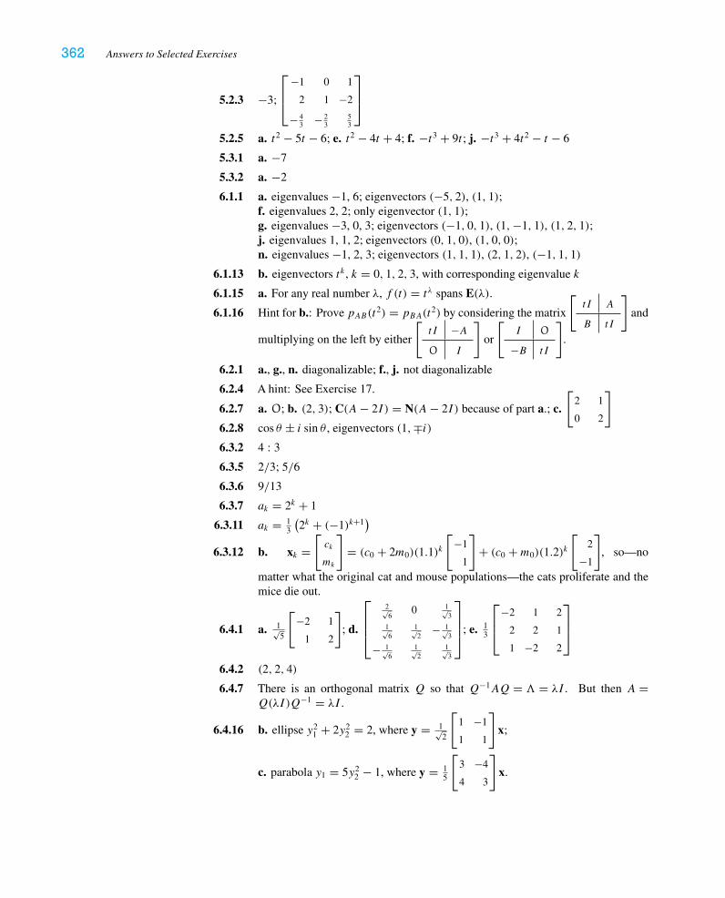
362 Answers to Selected Exercises
5.2.3 −3;
⎡⎢⎣
−1 0 1
2 1 −2
− 43 − 2
353
⎤⎥⎦
5.2.5 a. t2 − 5t − 6; e. t2 − 4t + 4; f. −t3 + 9t ; j. −t3 + 4t2 − t − 6
5.3.1 a. −7
5.3.2 a. −2
6.1.1 a. eigenvalues −1, 6; eigenvectors (−5, 2), (1, 1);f. eigenvalues 2, 2; only eigenvector (1, 1);g. eigenvalues −3, 0, 3; eigenvectors (−1, 0, 1), (1,−1, 1), (1, 2, 1);j. eigenvalues 1, 1, 2; eigenvectors (0, 1, 0), (1, 0, 0);n. eigenvalues −1, 2, 3; eigenvectors (1, 1, 1), (2, 1, 2), (−1, 1, 1)
6.1.13 b. eigenvectors tk , k = 0, 1, 2, 3, with corresponding eigenvalue k
6.1.15 a. For any real number λ, f (t) = tλ spans E(λ).
6.1.16 Hint for b.: Prove pAB(t2) = pBA(t2) by considering the matrix
[tI A
B tI
]and
multiplying on the left by either
[tI −AO I
]or
[I O
−B tI
].
6.2.1 a., g., n. diagonalizable; f., j. not diagonalizable
6.2.4 A hint: See Exercise 17.
6.2.7 a. O; b. (2, 3); C(A− 2I ) = N(A− 2I ) because of part a.; c.
[2 1
0 2
]
6.2.8 cos θ ± i sin θ , eigenvectors (1,∓i)6.3.2 4 : 3
6.3.5 2/3; 5/6
6.3.6 9/13
6.3.7 ak = 2k + 1
6.3.11 ak = 13
(2k + (−1)k+1
)
6.3.12 b. xk =[ck
mk
]= (c0 + 2m0)(1.1)k
[−1
1
]+ (c0 +m0)(1.2)k
[2
−1
], so—no
matter what the original cat and mouse populations—the cats proliferate and themice die out.
6.4.1 a. 1√5
[−2 1
1 2
]; d.
⎡⎢⎢⎣
2√6
0 1√3
1√6
1√2
− 1√3
− 1√6
1√2
1√3
⎤⎥⎥⎦; e. 1
3
⎡⎢⎣
−2 1 2
2 2 1
1 −2 2
⎤⎥⎦
6.4.2 (2, 2, 4)
6.4.7 There is an orthogonal matrix Q so that Q−1AQ = = λI . But then A =Q(λI)Q−1 = λI .
6.4.16 b. ellipse y21 + 2y2
2 = 2, where y = 1√2
[1 −1
1 1
]x;
c. parabola y1 = 5y22 − 1, where y = 1
5
[3 −4
4 3
]x.
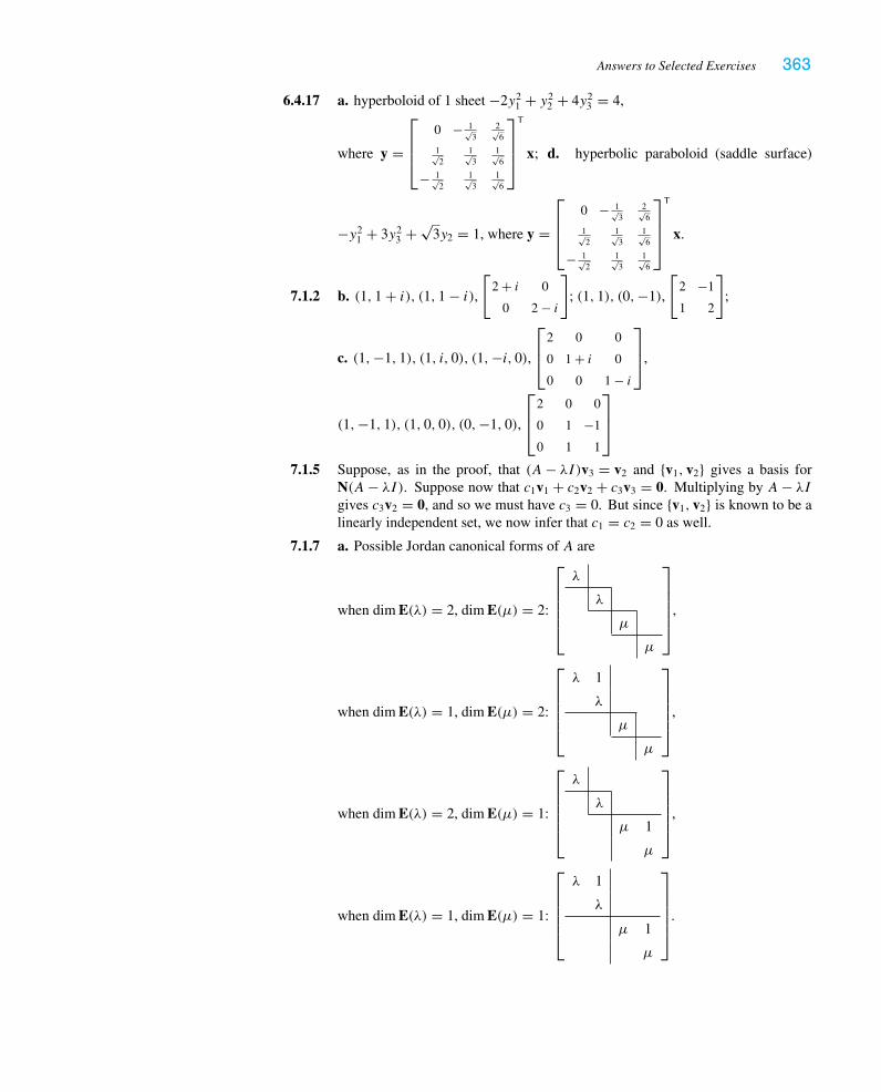
Answers to Selected Exercises 363
6.4.17 a. hyperboloid of 1 sheet −2y21 + y2
2 + 4y23 = 4,
where y =
⎡⎢⎢⎣
0 − 1√3
2√6
1√2
1√3
1√6
− 1√2
1√3
1√6
⎤⎥⎥⎦
T
x; d. hyperbolic paraboloid (saddle surface)
−y21 + 3y2
3 + √3y2 = 1, where y =
⎡⎢⎢⎣
0 − 1√3
2√6
1√2
1√3
1√6
− 1√2
1√3
1√6
⎤⎥⎥⎦
T
x.
7.1.2 b. (1, 1 + i), (1, 1 − i),[
2 + i 0
0 2 − i
]; (1, 1), (0,−1),
[2 −1
1 2
];
c. (1,−1, 1), (1, i, 0), (1,−i, 0),⎡⎢⎣
2 0 0
0 1 + i 0
0 0 1 − i
⎤⎥⎦,
(1,−1, 1), (1, 0, 0), (0,−1, 0),
⎡⎢⎣
2 0 0
0 1 −1
0 1 1
⎤⎥⎦
7.1.5 Suppose, as in the proof, that (A− λI)v3 = v2 and {v1, v2} gives a basis forN(A− λI). Suppose now that c1v1 + c2v2 + c3v3 = 0. Multiplying by A− λIgives c3v2 = 0, and so we must have c3 = 0. But since {v1, v2} is known to be alinearly independent set, we now infer that c1 = c2 = 0 as well.
7.1.7 a. Possible Jordan canonical forms of A are
when dim E(λ) = 2, dim E(μ) = 2:
⎡⎢⎢⎢⎢⎣
λ
λ
μ
μ
⎤⎥⎥⎥⎥⎦
,
when dim E(λ) = 1, dim E(μ) = 2:
⎡⎢⎢⎢⎢⎣
λ 1
λ
μ
μ
⎤⎥⎥⎥⎥⎦
,
when dim E(λ) = 2, dim E(μ) = 1:
⎡⎢⎢⎢⎢⎣
λ
λ
μ 1
μ
⎤⎥⎥⎥⎥⎦
,
when dim E(λ) = 1, dim E(μ) = 1:
⎡⎢⎢⎢⎢⎣
λ 1
λ
μ 1
μ
⎤⎥⎥⎥⎥⎦
.
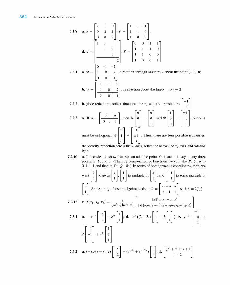
364 Answers to Selected Exercises
7.1.8 a. J =⎡⎢⎣
2 1 0
0 2 1
0 0 2
⎤⎥⎦, P =
⎡⎢⎣
1 −1 −1
1 1 0
1 0 0
⎤⎥⎦;
d. J =
⎡⎢⎢⎢⎢⎢⎣
1 1
1 1
1
2
⎤⎥⎥⎥⎥⎥⎦
, P =
⎡⎢⎢⎢⎣
0 0 1 1
1 −1 −1 0
1 1 0 0
1 0 0 1
⎤⎥⎥⎥⎦
7.2.1 a. =
⎡⎢⎢⎣
0 −1 −2
1 0 2
0 0 1
⎤⎥⎥⎦, a rotation through angle π/2 about the point (−2, 0);
b. =
⎡⎢⎢⎣
0 −1 2
−1 0 2
0 0 1
⎤⎥⎥⎦, a reflection about the line x1 + x2 = 2
7.2.2 b. glide reflection: reflect about the line x2 = 12 and translate by
[−1
0
]
7.2.3 a. If =[
A a
0 0 1
], then
⎡⎢⎣
0
0
1
⎤⎥⎦ =
⎡⎢⎣
0
0
1
⎤⎥⎦ and
⎡⎢⎣
1
0
0
⎤⎥⎦ =
⎡⎢⎣
±1
0
0
⎤⎥⎦. Since A
must be orthogonal,
⎡⎢⎣
0
1
0
⎤⎥⎦ =
⎡⎢⎣
0
±1
0
⎤⎥⎦. Thus, there are four possible isometries:
the identity, reflection across the x1-axis, reflection across the x2-axis, and rotationby π .
7.2.10 a. It is easiest to show that we can take the points 0, 1, and −1, say, to any threepoints, a, b, and c. (Then by composition of functions we can take P , Q, R to0, 1, −1 and then to P ′, Q′, R′.) In terms of homogeneous coordinates, then, we
want
[0
1
]to go to
[a
1
],
[1
1
]to multiple of
[b
1
], and
[−1
1
]to some multiple of
[c
1
]. Some straightforward algebra leads to =
[λb − a a
λ− 1 1
]with λ = 2 c−a
c−b .
7.2.12 c. f (x1, x2, x3) = 1√a2
1+a22
(a·(x−a)
)[
‖a‖2(a2x1 − a1x2)
‖a‖(a1a3x1 − a21x3 + a2(a3x2 − a2x3)
)]
7.3.1 a. −e−t[
−5
2
]+ e6t
[1
1
]; d. e2t
((2 − 3t)
[1
1
]− 3
[0
1
] ); e. e−3t
⎡⎢⎣
−1
0
1
⎤⎥⎦+
2
⎡⎢⎣
1
−1
1
⎤⎥⎦+ e3t
⎡⎢⎣
1
2
1
⎤⎥⎦
7.3.2 a. (− cos t + sin t)
[−5
2
]+ (e
√6t + e−
√6t )
[1
1
]; d.
[16 t
3 + t2 + 2t + 1
t + 2
]
Answers to Selected Exercises 365
7.3.3 c. normal modes e±it[
1
1
]and e±2it
[2
−1
]
7.3.4
⎡⎢⎣e2t te2t 1
2 t2e2t
0 e2t te2t
0 0 e2t
⎤⎥⎦
7.3.5 a. y(t) = e2t − 2e−t ; b. y(t) = et + tet

This page intentionally left blank

367
LIST OF BLUE BOXES
Topic Page
Grab paper and pencil 4Advice for geometric proofs 6Appearance of why? in text 8Language of sets 9When are two sets equal? 12Draw a sketch and decide what you really need to show 14What are you given and what do you need to show? 17Proof by contradiction and reduction to a special case 18Use properties rather than definition of dot product 20If and only if, and converse 21What does it mean to solve an equation? 23Specializing from the general 27Looking for examples and counterexamples 52The use of if in definitions 81The meaning of arbitrary 83Thinking of matrices as vectors 83Functions: domain, range, one-to-one, and onto 88Exploring matrix multiplication 90Working with nonsingular matrices 90Existence and uniqueness 91Examples don’t make a proof 92Verifying and disproving a multi-part definition 93, 128More on existence and uniqueness 124One-to-one functions 145The syntax of independence 146Whenever you must prove linear independence … 146Proof by contrapositive 148When are two numbers equal? 158Built-in check for eigenvalues 265

This page intentionally left blank

369
INDEX
affine subspace, 199affine transformation, 315angle, 23, 24, 182area, 255
signed, 256associative property, see matrix multiplication,
associative property
basis, 149, 179orthogonal, 200, 204orthonormal, 204, 287standard, 149, 184, 209
binomial theorem, 91
Cartesian equation, 8, 31cat/mouse, 70, 277Cauchy-Schwarz Inequality, 24, 27, 182Cavalieri’s principle, 256Cayley-Hamilton Theorem, 275, 314centroid, 17change-of-basis formula, 215change-of-basis matrix, 215, 231, 262characteristic polynomial, 265–267checkerboard, 247coefficients, 36cofactor, 247collinear, 10column space, 136
basis for, 161column vector, see vector, columncomplete induction, 309complex numbers, 299
multiplication of, 301complex vector space, 301conic section, 290–291conjugate, 299consistent, 55–58, 136constraint equation, 57, 114, 139, 163continuous functions, vector space of, 178contradiction, proof by, 18contrapositive, 148converse, 21, 148cookies, 25, 122coordinates, 150, 202cosine, power series of, 338counterexample, 52Cramer’s Rule, 250
cross product, 259curve fitting, 64–65cylinder, 291
derivative, 225determinant, 239, 240, 242diagonal, 82diagonalizable, 219, 261, 270, 273, 275, 276,
286simultaneously, 276, 296
difference equation, 69, 277differentiable, 178
continuously, 178differential equations, system of, 332–344dimension, 158direction, 1direction vector, 7discrete dynamical system, 70distance, 30, 32, 200distributive property, 19, 59, 87domain, 88dot product, 19, 313
echelon form, 43reduced, 43–47, 52
eigenspace, 263eigenvalue, 262
complex, 266, 302eigenvector, 74, 262
generalized, 314electric circuit, 67, 173elementary matrix, 111, 241elementary operations, 37elementary row operations, 41, 240ellipse, 291ellipsoid, 291equality of sets, proving, 12Euler’s formula, 339exponential series, 333
Fibonacci sequence, 74, 279finite-dimensional, 179Fred, 267Fred (and Barney), 72, 280free variable, 37, 43function
one-to-one, 88onto, 88

370 Index
function space, 176function, one-to-one, 145
Gauss-Jordan elimination, 53Gaussian elimination, 45, 104general solution, 32, 37, 45
standard form of, 45generalized eigenvector, 314Gerschgorin’s Circle Theorem, 313glide reflection, 321golden ratio, 280Gram-Schmidt process, 204graph, directed, 86, 171
homogeneous coordinate vector, 324homogeneous system, 59Hooke’s Law, 343hyperbola, 290hyperboloid, 291hyperplane, 32
identity map, 93identity matrix, 61, 87if and only if, 21image, 88, 136, 225imaginary part, 299implication, 21incidence matrix, 171inconsistent, 49, 55inconsistent system, 196
least squares solution, 193infinite-dimensional, 179inhomogeneous system, 59initial value, 332inner product space, 181intersection, 33, 37, 48, 56, 131, 135inverse matrix, 104
formula for, 106, 251left, 102right, 102
invertible, see matrix, invertibleisometry, 319
Jordan block, 307Jordan canonical form, 275, 306
exponential of, 341, 345
kernel, 225Kirchhoff’s laws, 67, 68, 173, 175
Lagrange interpolation, 65, 183leading entry, 43least squares line, 196least squares solution, 193, 197left inverse, 102left nullspace, 138
basis for, 161
length, 1, 10Leslie matrix, 71line, 7
of regression, 196linear combination, 11, 54
trivial, 145linear map, 92, 208, 224linear transformation, 91, 92, 208, 224
matrix for, 209, 228linearity properties, 92linearly dependent, 145, 179linearly independent, 145, 179loop, 68, 172LU decomposition, 116
Markov process, 280–284matrices
equality of, 39matrix, 39
addition, 82augmented, 41, 56block, 90, 109block diagonal, 304change-of-basis, 215, 231, 262diagonal, 82exponential, 333identity, 61, 87invertible, 104, 105, 108lower triangular, 82nonsingular, 61, 104, 105, 151, 241, 296orthogonal, 123, 206, 245permutation, 91positive (negative) definite, 296powers, 86product, 84, 110
not commutative, 85singular, 61skew-symmetric, 119square, 82standard, 98, 209symmetric, 119, 286upper (lower) triangular, 241upper triangular, 82zero, 82
matrix multiplication, see also matrix, productassociative property, 87, 89, 108, 120, 158distributive property, 59, 87
median, 6minimal polynomial, 314modulus, 299multiplicity
algebraic, 272, 305, 309geometric, 272, 305, 309
necessity, 21nilpotent, 276

Index 371
node, 67, 86, 171noncollinear, 10nonparallel, 3, 11nonsingular, see matrix, nonsingularnormal equations, 192normal mode, 336, 344normal vector, 28, 128nullity, 164Nullity-Rank Theorem, 165nullspace, 136
basis for, 160
Ohm’s Law, 67, 175orthogonal, 20
basis, 200, 204complement, 133, 165, 192matrix, see matrix, orthogonalset, 200subspaces, 134
orthonormal basis, 200, 204, 287
parabola, 293paraboloid, 294parallel, 3, 11, 147parallelogram law, 4parameter, 7parametric equation, 7, 11, 14, 32particular solution, 45, 59perpendicular, 19perspective projection, 322pivot, 43
column, 43variable, 37, 43
plane, 11polar form, 300polynomials, vector space of, 178power series, exponential, 333probability vector, 280, 281product, see dot product or matrix, productproduct rule, 241projection, 22, 121, 192, 202, 290
perspective, 322projection matrix, 194projective transformation, 324proof by contradiction, 18pun, atrocious, 219Pythagorean Theorem, 10, 20, 259
QR decomposition, 205, 266quadric surface, 291–294
range, 88rank, 46, 58, 164Rational Roots Test, 266real part, 299reduced echelon form, 43–47, 52
reflection, 94, 209, 319, 321reflection across �, 95reflection matrix, 95regression, line of, 196right inverse, 102rotation, 94, 321, 330rotation matrix, 98, 101, 102, 217–218rotatory reflection, 330row space, 138
basis for, 160row vector, see vector, row
scalar multiplication, 2, 10, 82scalar product, 19screw, 331set(s), 9
equality of, 12shear, 93, 314shoe-sock theorem, 108signed area, 256signed length, 23signed volume, 256similar, 219, 266sine, power series of, 338singular, see matrix, singularspan, 12, 129, 130, 179spectral decomposition, 290Spectral Theorem, 287standard basis, 149, 184, 209standard matrix, 209stochastic matrix, 281, 314stoichiometry, 66subset, 12subspace, 127, 177
affine, 199invariant, 307trivial, 128, 152
sufficiency, 21sum of subspaces, 132
trace, 186, 267transition matrix, 74, 280translation, 7, 59, 315, 319, 321transpose, 119, 172
determinant of, 242triangle inequality, 27, 313trivial solution, 60, 61trivial subspace, 128, 152
unique solution, 60, 61, 104unit vector, 2
variablefree, 43pivot, 43
vector, 1addition, 3

372 Index
column, 39, 53, 82commodity, 25homogeneous coordinate, 324normal, 28, 128price, 25probability, 281row, 39, 81
subtraction, 4unit, 2
vector addition, 10vector space, 176
finite-dimensional, 179infinite-dimensional, 179, 180
ViewPoint, 325