Linda PetzoldUniversity of California Santa Barbara

www.engineering.ucsb.edu/~cse

Definition: The understanding of biological network behavior through the application of modeling and simulation, tightly linked to experiment

GENOME NETWORK PHENOTYPE

• An ODE model cannot capture effects due to small numbers of key chemical species• A molecular dynamics model is too slow given the model complexities and time scales of interest

Why Spatially Inhomogeneous?

Why Discrete Stochastic Simulation?

Unfolded protein response in the endoplasmic reticulum – C. Young, A. Robinson, U. Delaware

Polarization in yeast mating – T. M. Yi, UC Irvine

Discrete stochastic simulation for well-mixed systems• Chemical master equation• Stochastic simulation algorithm (SSA)• Accelerated methods

•Tau-leaping• Hybrid• Slow-scale SSA• Finite state projection (FSP)

Discrete stochastic simulation for spatially inhomogeneous systems• Inhomogeneous SSA (ISSA)• Fundamental issues• Accelerated methods• Complicated geometries

Well-stirred mixture

N molecular species

Constant temperature, fixed volume

M reaction channels

Dynamical state where

is the number of molecules in the system

Propensity function the probability, given

that one reaction will occur

somewhere inside in the next infinitesimal time

interval

When that reaction occurs, it changes the state. The

amount by which changes is given by the

change in the number of molecules produced by one

reaction

is a jump Markov process

Draw two independent samples and from

and take

the smallest integer satisfying

Update X

Fast Formulations of SSA: Next Reaction method (Gibson & Bruck, 2000), Optimized Direct Method (Li & Petzold, 2004), Sorting Direct Method (McCollumna et al., 2004), Logarithmic Direct Method (Li & Petzold, 2006), Constant Time Method (Slepoy et al., 2008), SSA on GPU (Li & Petzold, 2009), Next Subvolume Method for ISSA (Elf & Ehrenberg, 2004)

Given a subinterval of length , if we could determine how many times each reaction channel fired in each subinterval, we could forego knowing the precise instants at which the firings took place. Thus we could leap from one subinterval to the next.

How long can that subinterval be? Tau-leaping is exact for constant propensity functions, thus is selected so that no propensity function changes ‘appreciably.’

Current implementations: Adaptive stepsize Non-negativity preserving Reverts to SSA when necessary

Hybrid methods Haseltine & Rawlings, 2002; Mattheyses, Kiehl & Simmons, 2002; Puchalka & Kierzek, 2004; Salis & Kaznessis, 2005; Rossinelli, Bayati & Koumatsakos, 2008 (ISSA)

Slow reactions involving species present in small numbers are simulated by SSA

Reactions where all constituents present with large populationsare simulated by reaction-rate equations

Cannot efficiently handle fast reactions involving species present in small numbers

Slow-Scale SSA (ssSSA) Cao, Petzold & Gillespie, 2004

Fast reactions, even those involving species present in very small numbers, can be treated with the stochastic partial equilibrium approximation (slow-scale SSA)

The CME describes the evolution of the probability density vector (PDV) for the system:

The CME is a large (possibly infinite) linear ODE.

Use a truncated state space with an absorbing state.

Solve directly. Absorbing state provides

a bound on the error.

•Munsky, J Chem Phys (2006)

• Introduce a discretization of the domain into subvolumes (voxels) and assume that the well-stirred assumption is fulfilled within each subvolume (green). Diffusion is introduced as jumps from one subvolume to adjacent subvolumes. • Cartesian, uniform mesh:

•Reaction part and diffusion part. The diffusion operator is given by influx and outflux of probability for each subvolume in the mesh (just as in the case for reactions).

•With q as on the previous slide and a uniform Cartesian mesh, we get convergence in mean to the solution of the macroscopic diffusion equation in the limit h -> 0. (Compare the 5-point stencil, finite difference method).

• The limit h -> 0 is not attainable for physical reasons. Condition on the mesh parameter h:

Elf & Ehrenberg, 2004For reaction-diffusion systems, for small enough h, molecules never react!Isaacson, 2009Theory and proposed improvement on algorithmErban & Chapman, 2009

• Propensities vary with molecular crowding, roughly as a function of the size of the moleculesLampoudi, Gillespie, Petzold, 2007, 2009Ellis, 2001; Despa, 2009

Huge computational complexity necessitates consideration of high performance computer architectures. However, large numbers of fast diffusive transfers puts severe limitation on speedup.

• Multinomial Simulation Algorithm (MSA) (Lampoudi, Gillespie, Petzold, 2008)

• Tau-leaping specifically adapted to diffusion: the propensities for diffusive transfers are conditional -> conservative

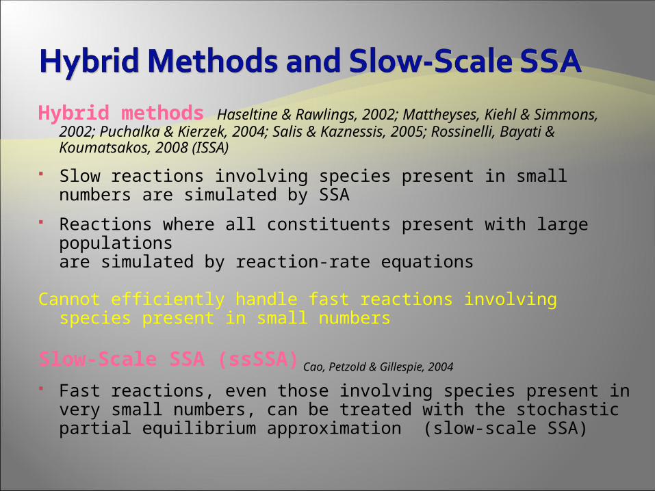
• Diffusion FSP (DFSP) (Drawert, Lawson, Khammash, Petzold, 2009)

• Diffusion of molecules originating in one voxel is independent of diffusion of molecules originating in all other voxels

Use truncated state space ( ) Solve: Note: Pick a random number against the

PDV Distribute molecules according to the

selected state

Well mixed assumption is violated by definition!

•Tau-Mu Yi, UC Irvine

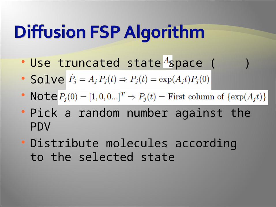
• Unstructured meshes and complicated geometries (Engblom, Ferm, Hellander, Lotstedt, 2009

• Well-stirred assumption in the subvolumes is determined by the dual of the Delauny triangulation (Voronoi cells)•Adaptive hybrid method, reactions by operator splitting (Ferm, Hellander, Lotstedt, 2009)•URDME software built on top of COMSOL Multiphysics•Currently limited in ability to handle stochastic stiffness

• Early work on complicated geometries (Isaacson & Peskin, 2006)

► Organelle surrounding nucleus -Lumen (interior) and -Large irregular membrane surface

•ER

•1 μm► “Gatekeeper” for proteins

Carissa Young, University of Delaware

Experimental Evidence for Spatial Localization

S. cerevisiae BJ5464 cells expressing fusion proteins BiP and Sec63 with various GFP variants. Images captured on Zeiss 5LIVE confocal microscope, Plan Apochromat 63x/ NA 1.40.

•BiP-Venus •Sec63-Cerulean •Merged Image

Carissa Young, University of Delaware

Concentration profile of total BiP on the ER membrane (left) and lumen (right) at simulation time t=5s

Currently investigating effectsof highly irregular ER geometry

Initial simulations of the spatial stochastic model produced variation in spatial concentrations due to stochastic fluctuations on both the membrane and the lumen, even though initial conditions were homogeneous.

Collaborators: Dan Gillespie, Frank Doyle, Anne Robinson, Mustafa Khammash, Tau-Mu Yi, Per Lotstedt, Andreas Hellander

Students: Min Roh, Marc Griesemer, Kevin Sanft, Brian Drawert, Michael Lawson

Former Students and Postdocs: Yang Cao, Muruhan Rathinam, Hong Li, Teri Lampoudi

Thanks!NSF, NSF IGERT, DOE, NIH, Army (ICB)