Embed Size (px)
Citation preview
Lifetime and Coverage Guarantees Through DistributedCoordinate-Free Sensor Activation
Gaurav S. KasbekarDepartment of Electrical and
Systems EngineeringUniversity of Pennsylvania
Philadelphia, PA, [email protected]
Yigal BejeranoBell-Labs, Alcatel-Lucent
Murray Hill, NJ, [email protected]
labs.com
Saswati SarkarDepartment of Electrical and
Systems EngineeringUniversity of Pennsylvania
Philadelphia, PA, [email protected]
ABSTRACTWireless Sensor Networks are emerging as a key sensingtechnology, with diverse military and civilian applications.In these networks, a large number of sensors perform dis-tributed sensing of a target field. Each sensor is a smallbattery-operated device that can sense events of interest inits sensing range and can communicate with neighboringsensors. A sensor cover is a subset of the set of all sensorssuch that every point in the target field is in the interior ofthe sensing ranges of at least k different sensors in the subset,where k is a given positive integer. The lifetime of the net-work is the time from the point the network starts operationuntil the set of all sensors with non-zero remaining energydoes not constitute a sensor cover. An important goal insensor networks is to design a schedule, that is, a sequenceof sensor covers to activate in every time slot, so as to max-imize the lifetime of the network. In this paper, we design apolynomial-time, distributed algorithm for maximizing thelifetime of the network and prove that its lifetime is at mosta factor O(log n ∗ log nB) lower than the maximum possiblelifetime, where n is the number of sensors and B is an upperbound on the initial energy of each sensor. Our algorithmdoes not require knowledge of the locations of nodes or di-rectional information, which is difficult to obtain in sensornetworks. Each sensor only needs to know the distancesbetween adjacent nodes in its transmission range and theirsensing radii. In every slot, the algorithm first assigns aweight to each node that is exponential in the fraction of itsinitial energy that has been used up so far. Then, in a dis-tributed manner, it finds a O(log n) approximate minimumweight sensor cover which it activates in the slot. Our simu-lations reveal that our algorithm substantially outperformsseveral existing lifetime maximization algorithms.
Categories and Subject DescriptorsC.2.1 [Network Architecture and Design]: Wireless com-munication
Permission to make digital or hard copies of all or part of this work forpersonal or classroom use is granted without fee provided that copies arenot made or distributed for profit or commercial advantage and that copiesbear this notice and the full citation on the first page. To copy otherwise, torepublish, to post on servers or to redistribute to lists, requires prior specificpermission and/or a fee.MobiCom’09, September 20–25, 2009, Beijing, China.Copyright 2009 ACM 978-1-60558-702-8/09/09 ...$10.00.
General TermsAlgorithms, Design, Performance, Theory
KeywordsWireless Sensor Networks, Network Lifetime, Coverage, Ap-proximation Algorithms, Distributed Algorithms, Coordinate-Free
1. INTRODUCTIONRecent advances in wireless communications and electron-
ics have enabled the development of low-cost sensor nodes [12].Each sensor node is capable of sensing specific events in itsvicinity and of communicating with adjacent nodes. Thus,for event sensing applications, a large number of sensor nodesare deployed in a distribution area and they collaborate toform an ad-hoc network, referred to as a wireless sensor net-work (WSN). WSNs have the potential to become the domi-nant sensing technology in many civilian and military appli-cations, such as intrusion detection, environmental monitor-ing, object tracking, traffic control, and inventory manage-ment. In many of these applications, WSNs need to monitorthe target field for detecting events of interest, e.g., entranceof an intruder in an intrusion detection application.
Wide-spread deployment of WSNs in target field monitor-ing is being deterred by the energy consumed in the mon-itoring process. The challenge is compounded by the factthat the sensors are battery-powered and owing to size lim-itations the sensors can only be deployed with low-lifetimebatteries, most of which are not rechargeable. Thus, a sen-sor ceases to function (e.g., monitor) once its battery ex-pires, and oftentimes, sensors whose batteries have expiredcan not be easily replaced owing to logistics issues such asremoteness or inaccessibility of distribution areas. Thus, thesuccess of the WSN technology is contingent upon develop-ing strategies for intelligently using the available sensors soas to maximize the duration for which the entire target fieldis monitored by sensors. This duration, referred to as thenetwork lifetime, is an important performance metric for thenetwork as the coverage of the entire target field is essentialfor reliable detection of events of interest.
Owing to large scale availability of low cost sensors, sen-sors are often deployed with some redundancy, that is, sev-eral locations in the target field can be monitored by mul-tiple sensors. Lifetime of the WSNs can be substantiallyenhanced by intelligently activating the sensors that mon-itor the target field at any given time. We seek to maxi-
mize the lifetime of sensor networks by designing algorithmsthat dynamically activate sensors based on their residualenergy content. The algorithm we develop is completelydistributed, does not need to know the coordinates of anysensor, and provides provable guarantees on the attainedlifetimes.
1.1 Related LiteratureCoverage, connectivity and lifetime maximization for WSNs
have received considerable attention in the last few years.Comprehensive surveys can be found in [14, 15]. Most ofthe existing papers focus on the coverage and connectivityaspects [2, 16, 17, 18, 6, 10, 19, 20, 21], and typically pro-pose computational geometry based approaches for discover-ing coverage holes and ensuring connectivity. An interestingconnectivity property has been proved in [20, 21] that showsthat if the trasmission radius of each node is at least twice ofits sensing radius, then coverage implies connectivity of thesensor network. We make the same assumption, and there-fore seek to maximize lifetime while guaranteeing coveragewithout explicitly considering connectivity.
We now summarize the papers that propose topology con-trol solutions that maximize the network lifetime by schedul-ing the active periods of the sensors, while preserving cover-age and connectivity requirements. In [13] Cardei et al. ad-dress the problem of lifetime maximization when only agiven set of targets needs to be covered. They showed thatthe problem is NP-hard and provided heuristic sensor acti-vation algorithms based on linear programming relaxations.They also proposed a greedy heuristic activation scheme thatat each round seeks the minimal set of sensors that coversall the targets. They evaluated the lifetimes attained by theheuristic solutions using simulations, but did not provideprovable guarantees on the lifetimes of these schemes. To ourknowledge, the only scheme that provides guarantees on thenetwork lifetime is the one proposed by Berman et al. [11].They have provided a centralized algorithm that attains anetwork lifetime which is within O(log n) of the maximumpossible lifetime, where n is the number of sensors. Thisalgorithm determines how to activate sensors based on anapproximate solution of a linear program that requires com-plete knowledge of network topology, coordinates of sensorlocations and initial energy of sensors. Such linear programscan clearly be solved only by a central entity that knows allof the above, which is hard to realize in practice. Also, thesensors rarely know their precise locations since WSNs usu-ally do not have access to global positioning systems (GPS).Several sensor positioning systems [23, 24] have been pro-posed in the literature for learning the locations, withoutmanual configuration or the use of GPS receivers. However,they provide only coarse location estimations in practicalsettings [25]. Note that several coverage verification algo-rithms that do not assume knowledge regarding the locationsof the sensors exist [17, 16, 10, 3], but these papers do notprovide any guarantee on the network lifetime. Our con-tribution is to provide a distributed, coordinate-free sensoractivation scheme that provides provable guarantees on thenetwork lifetime.
Finally, Wu et al. [22] considered a different notion of life-time in a recent paper: the maximum time until which allnodes in the data aggregation tree of choice remain oper-ational, (a node in this case consumes energy only duringcommunication). Since we focus on the energy consumed in
sensing, our notion of lifetime, the problem formulation andsolution techniques differ substantially.
1.2 Our ContributionThe contribution of this paper is two-fold.First, we present the first coordinate-free distributed scheme
that provides provable approximation guarantees on networklifetime, while providing strict coverage guarantees. This isa surprising result since the sensors are not aware of theircoordinates in a global coordinate system, and are there-fore oblivious to their locations relative to each other and tothe target field. To overcome this challenge we assume thatthe sensor distribution area is slightly larger than the areathat needs to be monitored. The sensors are divided intoperiphery nodes that are located near the boundary of thedistribution area and internal nodes that are internal to thisarea. The target field that our scheme is committed to mon-itor is taken as the closure of the area covered by the internalnodes. Our scheme at each time slot selects a subset of sen-sors for monitoring the target field that ensure k-coverage ofthe entire target field, for a given integer k ≥ 1, and differ-ent subsets may be selected in different slots. The selectionprocess relies on two key steps: (i) each sensor is assigneda weight that is an exponentially increasing function of theenergy it has consumed so far (ii) the set of sensors thathas the minimum total weight, or an approximation thereof,among all those that cover the entire target field is acti-vated. This selection process balances the monitoring loadon all the sensors, and preferentially selects in each slot thesensors with high residual energy. We demonstrate that thealgorithm can be executed using distributed computationsthat do not need to know the locations of the sensors.
Second, we prove that the lifetime of the network whenthis algorithm is used is at least 1/O((log n)(log nB)) of theoptimal solution, where n is the number of sensors and Bis a bound on the initial energy level of the nodes. Weprove this approximation ratio, by extending to this problemthe exponential-function technique, originally developed byAspnes et al. [26] in the context of online machine schedulingand virtual circuit routing and later used by Awerbuch etal. [4] in on-line virtual circuit routing. Thus, our algorithmattains a provable guarantee which is only slightly worse ascompared with the best available centralized performanceguarantee till date, presented in [11]. We demonstrate viasimulations that our scheme attains a significantly higherlifetime than several other existing schemes [11, 21, 13].
2. PRELIMINARY
2.1 Network ModelWe consider a wireless sensor network (WSN) consisting
of a set S of n sensors that are also called nodes. Eachnode u ∈ S can sense events of interest in its sensing rangeand communicate with nodes in its transmission range. Wemake the natural assumption that there are no two sensorsat the same location. Also, each sensor u ∈ S has a uniqueidentification number, denoted by ID(u). The sensors aredistributed over a large 2-dimensional area. We refer to theregion obtained by the union of the sensing ranges of all thesensors as the distribution area and it subsumes the regionthat needs to be monitored by the sensors, referred to as themonitoring area. The latter is typically significantly largerthan the sensing range of a single sensor.
We assume that the sensing and transmission ranges of anode u are open discs, centered at u, with radii ru and Ru
respectively, where Ru > ru. Let r = maxu∈S ru, and R =minu∈S Ru. The boundary of the sensing range of any nodeu is a circle, which we refer to as the sensing border of nodeu. Let du,v denote the Euclidean distance between nodes uand v. Nodes u and v are termed adjacent or neighbors ifthey are included in the transmission range of each other.Let Nu be the set of neighbors of u.
We assume that nodes only have localized distance infor-mation. Specifically, each node u knows (a) ru, (b) du,v andrv for each v ∈ Nu and (c) dv,w for each pair w, v ∈ Nu
such that w and v are neighbors of each other. Thus, weassume that each node can estimate its sensing radius, andits distances from its neighbors without learning their orien-tations, and communicates this information to its neighbors.Note that recent studies [8, 9] have introduced accurate dis-tance estimation techniques that are applicable to wirelesssensors.
We assume that there is a periphery band of width atleast r between the boundary of the distribution area andthe edge of the monitoring area. We distinguish betweenperiphery nodes that are located in the periphery band andinternal nodes that lie in the monitoring area. Althoughthe sensors are not aware of their locations, we assume thatevery sensor knows if it is a periphery or an internal node,for instance by using the mechanisms in [6, 7].
The time is divided into time slots and we assume thatthe sensors have synchronized clocks which notify them atthe beginning of each time slot. Sensor u ∈ S has an initialenergy Bu and, as a normalization, we assume that eachsensor consumes 1 unit of energy in each time slot in whichit is active. For saving energy, a sensor may be in a sleepmode, in which it does not communicate with its neighborsnor sense its vicinity. A sensor in sleep mode consumes onlynegligible amount of energy, which we assume to be zero.
2.2 The Target Field
An internal node &
its sensing range A periphery node &
its sensing range
The distribution area
The monitoring area
The target field
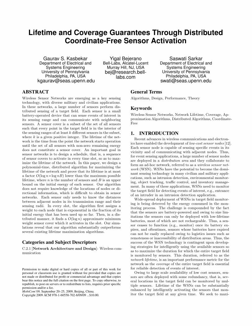
Figure 1: An example of a small WSN and its targetfield.
Generally speaking, the target field is the area monitoredby the system. This area is obviously subsumed in the dis-tribution area and it should contain the monitoring area.Since the sensors are not aware of their locations, they are
oblivious to their locations relative to each other and to themonitoring area. Addressing this difficulty, we next providea precise definition of the target field that our scheme iscommitted to monitor.
Definition 1 (The Target Field). The target fieldis the area defined by the closure 1 of the union of the sensingranges of all the internal sensors.
We assume that the target field subsumes the monitor-ing area. Figure 1 illustrates a small WSN as well as itsdistribution area, monitoring area and target field.
Given a set C ⊆ S of sensors and a positive integer k, wesay that a point in the target field is k-covered by C if itis in the interior of the sensing range of at least k nodes inC. The target field is considered as k-covered by C if everypoint in the target field is k-covered by C.
Definition 2 (Sensor Cover). A set C of sensors thatk-covers the target field is termed a sensor cover.
If there does not exist a sensor cover C such that all thenodes in C have non-zero energy, then the network is saidto have a coverage hole.
Since the sensing ranges are open discs, no sensor coversits sensing border. Thus, any sensor cover must containperiphery sensors that cover the target-field boundary (seeFig. 1). Thus, sensor activation schemes must consider bothinternal and periphery nodes.
2.3 Problem StatementWe proceed to define the maximum network lifetime prob-
lem.
Definition 3 (The Network Lifetime). The networklifetime is the time interval from the activation of the net-work until the first time at which a coverage hole appears.
Definition 4. (The Maximum Network Lifetime Prob-lem) An activation schedule is a sequence of sensor coversthat are activated in successive slots, such that in every slot,each sensor in the activated sensor cover has non-zero en-ergy. The maximum network lifetime problem seeks to findan activation schedule that maximizes the network lifetime.
In [13], the authors prove that the closely-related targetcoverage version of the maximum network lifetime problemis NP-hard. Moreover, in [10] it has been shown that fora given subset C ⊆ S, no coordinate-free algorithm canprovably verify whether or not C covers the target field,if R < 2r. So henceforth, we assume that R ≥ 2r andwe present a distributed coordinate-free algorithm for themaximum network lifetime problem with guarantee on thelifetime attained by the calculated schedule.
2.4 The Intersection Point ConceptWe now present an observation that constitutes a corner-
stone in our solution. Consider two sensors v, z ∈ S. Thesensors are termed intersecting if their sensing borders in-tersect (but not tangent to each other). In such case, we saythat v intersects with z.
1Recall that the closure of a set A is the smallest closed setthat contains A [27].
Property 1 (Intersection). The sensors v, z ∈ S areintersecting if and only if dv,z < rv + rz, dv,z + rz > rv anddv,z + rv > rz.
Note that the sensing borders of any pair v, z ∈ S of inter-secting sensors have exactly two intersection points denotedby IP (v, z, 1) and IP (v, z, 2). Moreover, by Property 1,since the distance dv,z < rv + rz ≤ 2 · r and we assume
that R ≥ 2 · r, any two intersecting sensors v, z are adjacent.We next show that for calculating a sensor cover we just
need to consider sensors that have intersection points ontheir sensing borders.
Property 2. Consider a sensor cover C ⊂ S and letu ∈ C be a sensor without any intersection point on itssensing border. Then the set C−{u} is also a sensor cover.
Proof. A necessary condition for the target field to bek-covered by C is that every point in the target field is in theinterior of the sensing ranges of at least k sensors in C. Sincewe assume that the target field is larger than the sensingrange of any single sensor, the set C contains additionalsensors beside u. Since u’s sensing border does not intersectwith that of any other sensor in C, then to ensure coverageof the target field, either (a) the sensing range of u does notcover any part of the target field or (b) u’s sensing rangeis subsumed in the sensing ranges of k other sensors, sayv1, . . . , vk, in C, and hence v1, . . . , vk cover the part of thetarget field covered by u. Thus, in both cases C − {u} isalso a sensor cover.
The next corollary directly follows from Property 2.
Corollary 1. Let u ∈ S be a sensor without any inter-section point on its sensing border and consider a schedule{C1, C2, · · · , CL} of sensor covers with network lifetime ofL in which node u is active in some slots. Then, the sched-ule {C1, C2, · · · , CL}, where Cj = Cj − {u}, also defines asequence of sensor covers with network lifetime of L.
From Corollary 1 it follows that the network lifetime isnot affected by ignoring sensors without intersection pointson their sensing borders. So henceforth, we will ignore suchsensors.
Let P be the set of intersection points that are in thetarget field, referred to as the IP set. Recall that P containsevery intersection point IP (v, z, i), i = {1, 2}, such thatat least one of the nodes v, z ∈ S is an internal node orIP (v, z, i) is in the sensing range of an internal node.
Theorem 1. Consider a set C ⊂ S of sensors. The setC is a sensor cover if and only if it k-covers every point inthe IP set P .
Proof. If C k-covers the target field, then by definitionit k-covers every point in P .
To prove the converse, suppose C k-covers every point inP . First, we prove that every point in the target field thatlies on the sensing border of some sensor is k-covered by C.Let f be a point in the target field on sensor v’s sensingborder. If f is an intersection point, it is k-covered by C,by assumption. If not, trace a path from f along v’s sensingborder to first reach an intersection point, say e. Recallthat every sensor that we consider has an intersection pointon its sensing border. So there exists such a point e. By
definition of the target field, e lies in the target field andhence, by assumption, is k-covered by C. Also, the pathtraced from f to e did not cross the sensing border of anysensor because the path first reached any intersection pointat e. So it follows that f is in the interior of the sensingranges of exactly the same subset of sensors of C as e is in 2,and hence is k-covered by C.
Now, let h be any point in the target field. If h lies on thesensing border of some sensor, it is k-covered by C, as shownabove. If not, trace a path from h to first reach the sensingborder of some sensor at some point, say g. By definition ofthe target field, g lies in the target field. Hence, as shownabove, g is k-covered by C and by arguments similar to thosein the previous paragraph, h is also k-covered by C.
Owing to Theorem 1, we henceforth consider as sensorcover any set of sensors that k-covers all the intersectionpoints in P .
3. ALGORITHM OVERVIEWWe now describe the Distributed Lifetime Maximization
(DLM) algorithm that we propose. In this section, we presenta brief overview of the individual building blocks in DLM,and provide the details in Sections 4, 5.
Our algorithm consists of an initialization phase and anactivation phase. The initialization phase is executed once,at the beginning of the network operation, and informs thenodes of some network-parameters. Every node executesthe activation phase at the beginning of each subsequenttime slot, and decides whether to activate itself in the slotbased only on the state information in its neighborhood.We now describe the above phases, and introduce some newterminologies towards that end.
Consider a sensor cover C, and let sensor u have weightwu, a positive real number. The weight of the sensor cover Cis the sum of the weights of the sensors in C, i.e.,
∑u∈C wu.
Definition 5 (A minimum weight sensor cover). Aminimum weight sensor cover is a sensor cover that has theminimum weight among all sensor covers. An α−approximateminimum weight sensor cover is one whose weight is at mostα times that of the minimum weight sensor cover.
Let Pu be the set of intersection points covered by sensoru, and Tu be the set of sensors v such that sensors u and vcover a common intersection point.
3.1 Initialization phaseAn initialization phase is executed at the beginning of
the network operation, i.e., at time t = 0. During the ini-tialization phase, each sensor u acquires the following localinformation: (i) the set Pu of intersection points that itcovers, (ii) the identities of the sensors in Tu and (iii) theintersection points in Pu that are covered by each sensorin Tu (i.e., the set Pu,v = Pu ∩ Pv for each v ∈ Tu). Aswe elaborate in Section 5, each sensor u learns this infor-mation in a distributed manner by merely communicatingwith its neighbors and using only localized distance informa-tion. In addition, each sensor learns the following global net-work parameters: (i) n, the total number of sensors, and (ii)the maximum amount B of the initial energy of any sensor
2Recall that the sensing range of each node is an open disc.
(B = maxu∈S Bu). Using the above information, each sen-sor computes µ, where µ = 4nB. The above constitutes theonly global information each sensor needs to know through-out the execution of DLM, and can be communicated toeach sensor using one network-wide broadcast.
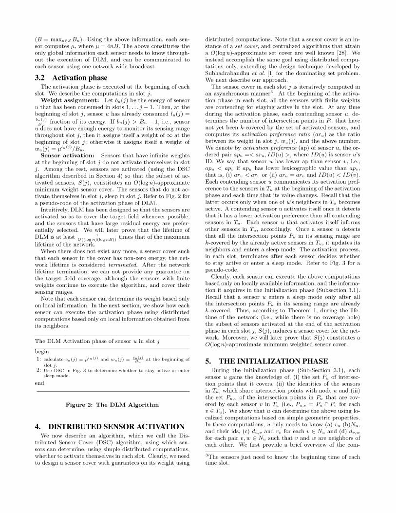
3.2 Activation phaseThe activation phase is executed at the beginning of each
slot. We describe the computations in slot j.Weight assignment: Let bu(j) be the energy of sensor
u that has been consumed in slots 1, . . . j − 1. Then, at thebeginning of slot j, sensor u has already consumed lu(j) =bu(j)Bu
fraction of its energy. If bu(j) > Bu − 1, i.e., sensoru does not have enough energy to monitor its sensing rangethroughout slot j, then it assigns itself a weight of ∞ at thebeginning of slot j; otherwise it assigns itself a weight ofwu(j) = µlu(j)/Bu.
Sensor activation: Sensors that have infinite weightsat the beginning of slot j do not activate themselves in slotj. Among the rest, sensors are activated (using the DSCalgorithm described in Section 4) so that the subset of ac-tivated sensors, S(j), constitutes an O(log n)-approximateminimum weight sensor cover. The sensors that do not ac-tivate themselves in slot j, sleep in slot j. Refer to Fig. 2 fora pseudo-code of the activation phase of DLM.
Intuitively, DLM has been designed so that the sensors areactivated so as to cover the target field whenever possible,and the sensors that have large residual energy are prefer-entially selected. We will later prove that the lifetime ofDLM is at least 1
O((log n)(log nB))times that of the maximum
lifetime of the network.When there does not exist any more, a sensor cover such
that each sensor in the cover has non-zero energy, the net-work lifetime is considered terminated. After the networklifetime termination, we can not provide any guarantee onthe target field coverage, although the sensors with finiteweights continue to execute the algorithm, and cover theirsensing ranges.
Note that each sensor can determine its weight based onlyon local information. In the next section, we show how eachsensor can execute the activation phase using distributedcomputations based only on local information obtained fromits neighbors.
The DLM Activation phase of sensor u in slot j
begin
1: calculate cu(j) = µlu(j) and wu(j) =cu(j)
Buat the beginning of
slot j.2: Use DSC in Fig. 3 to determine whether to stay active or enter
sleep mode.
end
Figure 2: The DLM Algorithm
4. DISTRIBUTED SENSOR ACTIVATIONWe now describe an algorithm, which we call the Dis-
tributed Sensor Cover (DSC) algorithm, using which sen-sors can determine, using simple distributed computations,whether to activate themselves in each slot. Clearly, we needto design a sensor cover with guarantees on its weight using
distributed computations. Note that a sensor cover is an in-stance of a set cover, and centralized algorithms that attaina O(log n)-approximate set cover are well known [28]. Weinstead accomplish the same goal using distributed compu-tations only, extending the design technique developed bySubhadrabandhu et al. [1] for the dominating set problem.We next describe our approach.
The sensor cover in each slot j is iteratively computed inan asynchronous manner3. At the beginning of the activa-tion phase in each slot, all the sensors with finite weightsare contending for staying active in the slot. At any timeduring the activation phase, each contending sensor u, de-termines the number of intersection points in Pu that havenot yet been k-covered by the set of activated sensors, andcomputes its activation preference ratio (aru) as the ratiobetween its weight in slot j, wu(j), and the above number.We denote by activation preference (ap) of sensor u, the or-dered pair apu =< aru, ID(u) >, where ID(u) is sensor u’sID. We say that sensor u has lower ap than sensor v, i.e.,apu < apv if apu has lower lexicographic value than apv,that is, (i) aru < arv or (ii) aru = arv and ID(u) < ID(v).Each contending sensor u communicates its activation pref-erence to the sensors in Tu at the beginning of the activationphase and each time that its value changes. Recall that thelatter occurs only when one of u’s neighbors in Tu becomesactive. A contending sensor u activates itself once it detectsthat it has a lower activation preference than all contendingsensors in Tu. Each sensor u that activates itself informsother sensors in Tu, accordingly. Once a sensor u detectsthat all the intersection points Pu in its sensing range arek-covered by the already active sensors in Tu, it updates itsneighbors and enters a sleep mode. The activation process,in each slot, terminates after each sensor decides whetherto stay active or enter a sleep mode. Refer to Fig. 3 for apseudo-code.
Clearly, each sensor can execute the above computationsbased only on locally available information, and the informa-tion it acquires in the Initialization phase (Subsection 3.1).Recall that a sensor u enters a sleep mode only after allthe intersection points Pu in its sensing range are alreadyk-covered. Thus, according to Theorem 1, during the life-time of the network (i.e., while there is no coverage hole)the subset of sensors activated at the end of the activationphase in each slot j, S(j), induces a sensor cover for the net-work. Moreover, we will later prove that S(j) constitutes aO(log n)-approximate minimum weighted sensor cover.
5. THE INITIALIZATION PHASEDuring the initialization phase (Sub-Section 3.1), each
sensor u gains the knowledge of, (i) the set Pu of intersec-tion points that it covers, (ii) the identities of the sensorsin Tu, which share intersection points with node u and (iii)the set Pu,v of the intersection points in Pu that are cov-ered by each sensor v in Tu (i.e., Pu,v = Pu ∩ Pv for eachv ∈ Tu). We show that u can determine the above using lo-calized computations based on simple geometric properties.In these computations, u only needs to know (a) ru (b)Nu,and their ids, (c) du,v and rv for each v ∈ Nu and (d) dv,w
for each pair v, w ∈ Nu such that v and w are neighbors ofeach other. We first provide a brief overview of the com-
3The sensors just need to know the beginning time of eachtime slot.
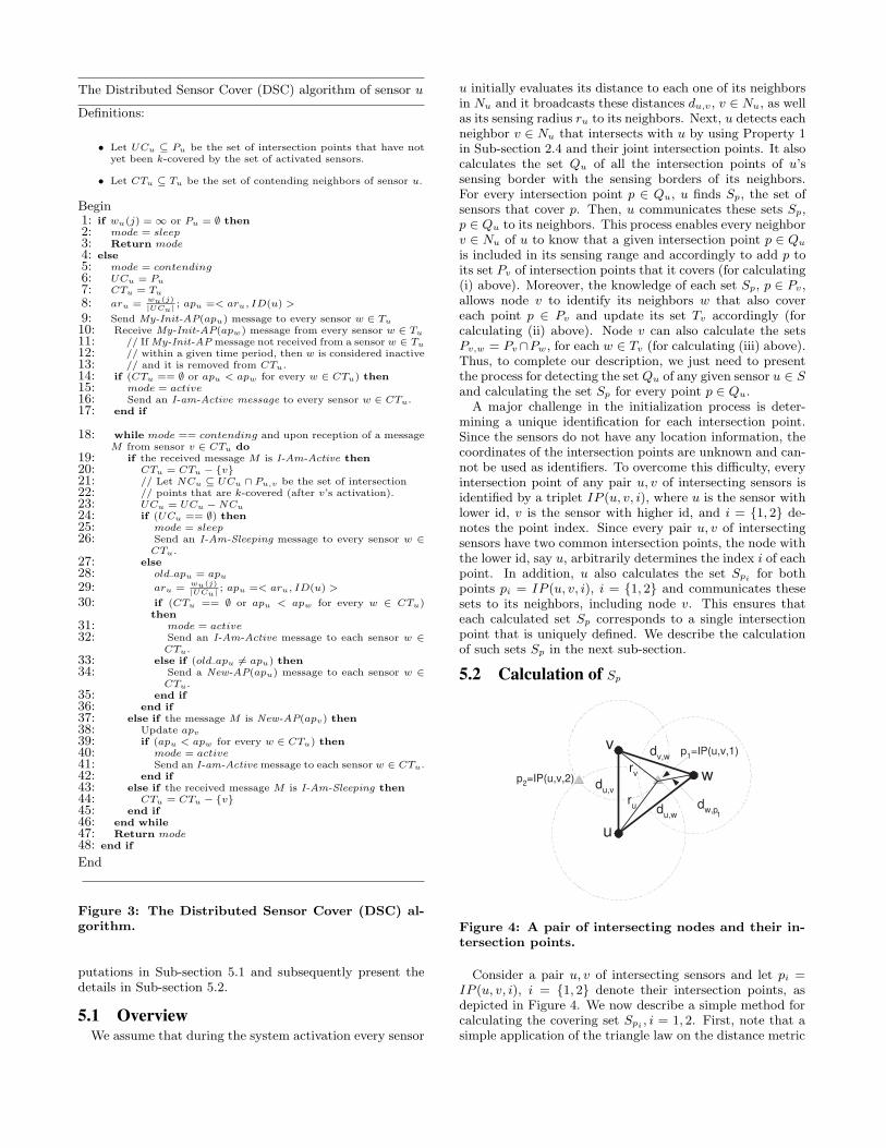
The Distributed Sensor Cover (DSC) algorithm of sensor u
Definitions:
• Let UCu ⊆ Pu be the set of intersection points that have notyet been k-covered by the set of activated sensors.
• Let CTu ⊆ Tu be the set of contending neighbors of sensor u.
Begin1: if wu(j) = ∞ or Pu = ∅ then2: mode = sleep3: Return mode4: else5: mode = contending6: UCu = Pu
7: CTu = Tu
8: aru =wu(j)|UCu| ; apu =< aru, ID(u) >
9: Send My-Init-AP(apu) message to every sensor w ∈ Tu
10: Receive My-Init-AP(apw) message from every sensor w ∈ Tu
11: // If My-Init-AP message not received from a sensor w ∈ Tu
12: // within a given time period, then w is considered inactive13: // and it is removed from CTu.14: if (CTu == ∅ or apu < apw for every w ∈ CTu) then15: mode = active16: Send an I-am-Active message to every sensor w ∈ CTu.17: end if
18: while mode == contending and upon reception of a messageM from sensor v ∈ CTu do
19: if the received message M is I-Am-Active then20: CTu = CTu − {v}21: // Let NCu ⊆ UCu ∩ Pu,v be the set of intersection22: // points that are k-covered (after v’s activation).23: UCu = UCu −NCu
24: if (UCu == ∅) then25: mode = sleep26: Send an I-Am-Sleeping message to every sensor w ∈
CTu.27: else28: old apu = apu
29: aru =wu(j)|UCu| ; apu =< aru, ID(u) >
30: if (CTu == ∅ or apu < apw for every w ∈ CTu)then
31: mode = active32: Send an I-Am-Active message to each sensor w ∈
CTu.33: else if (old apu 6= apu) then34: Send a New-AP(apu) message to each sensor w ∈
CTu.35: end if36: end if37: else if the message M is New-AP(apv) then38: Update apv
39: if (apu < apw for every w ∈ CTu) then40: mode = active41: Send an I-am-Active message to each sensor w ∈ CTu.42: end if43: else if the received message M is I-Am-Sleeping then44: CTu = CTu − {v}45: end if46: end while47: Return mode48: end if
End
Figure 3: The Distributed Sensor Cover (DSC) al-gorithm.
putations in Sub-section 5.1 and subsequently present thedetails in Sub-section 5.2.
5.1 OverviewWe assume that during the system activation every sensor
u initially evaluates its distance to each one of its neighborsin Nu and it broadcasts these distances du,v, v ∈ Nu, as wellas its sensing radius ru to its neighbors. Next, u detects eachneighbor v ∈ Nu that intersects with u by using Property 1in Sub-section 2.4 and their joint intersection points. It alsocalculates the set Qu of all the intersection points of u’ssensing border with the sensing borders of its neighbors.For every intersection point p ∈ Qu, u finds Sp, the set ofsensors that cover p. Then, u communicates these sets Sp,p ∈ Qu to its neighbors. This process enables every neighborv ∈ Nu of u to know that a given intersection point p ∈ Qu
is included in its sensing range and accordingly to add p toits set Pv of intersection points that it covers (for calculating(i) above). Moreover, the knowledge of each set Sp, p ∈ Pv,allows node v to identify its neighbors w that also covereach point p ∈ Pv and update its set Tv accordingly (forcalculating (ii) above). Node v can also calculate the setsPv,w = Pv∩Pw, for each w ∈ Tv (for calculating (iii) above).Thus, to complete our description, we just need to presentthe process for detecting the set Qu of any given sensor u ∈ Sand calculating the set Sp for every point p ∈ Qu.
A major challenge in the initialization process is deter-mining a unique identification for each intersection point.Since the sensors do not have any location information, thecoordinates of the intersection points are unknown and can-not be used as identifiers. To overcome this difficulty, everyintersection point of any pair u, v of intersecting sensors isidentified by a triplet IP (u, v, i), where u is the sensor withlower id, v is the sensor with higher id, and i = {1, 2} de-notes the point index. Since every pair u, v of intersectingsensors have two common intersection points, the node withthe lower id, say u, arbitrarily determines the index i of eachpoint. In addition, u also calculates the set Spi for bothpoints pi = IP (u, v, i), i = {1, 2} and communicates thesesets to its neighbors, including node v. This ensures thateach calculated set Sp corresponds to a single intersectionpoint that is uniquely defined. We describe the calculationof such sets Sp in the next sub-section.
5.2 Calculation of Sp
v
u
w
p 1 =IP(u,v,1)
p 2 =IP(u,v,2)
d u,v
d u,w
d v,w
r v
r u d
w,p 1
Figure 4: A pair of intersecting nodes and their in-tersection points.
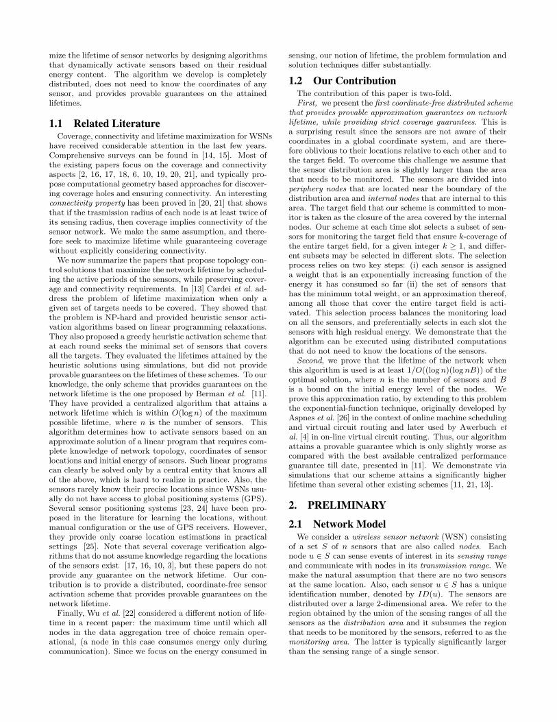
Consider a pair u, v of intersecting sensors and let pi =IP (u, v, i), i = {1, 2} denote their intersection points, asdepicted in Figure 4. We now describe a simple method forcalculating the covering set Spi , i = 1, 2. First, note that asimple application of the triangle law on the distance metric
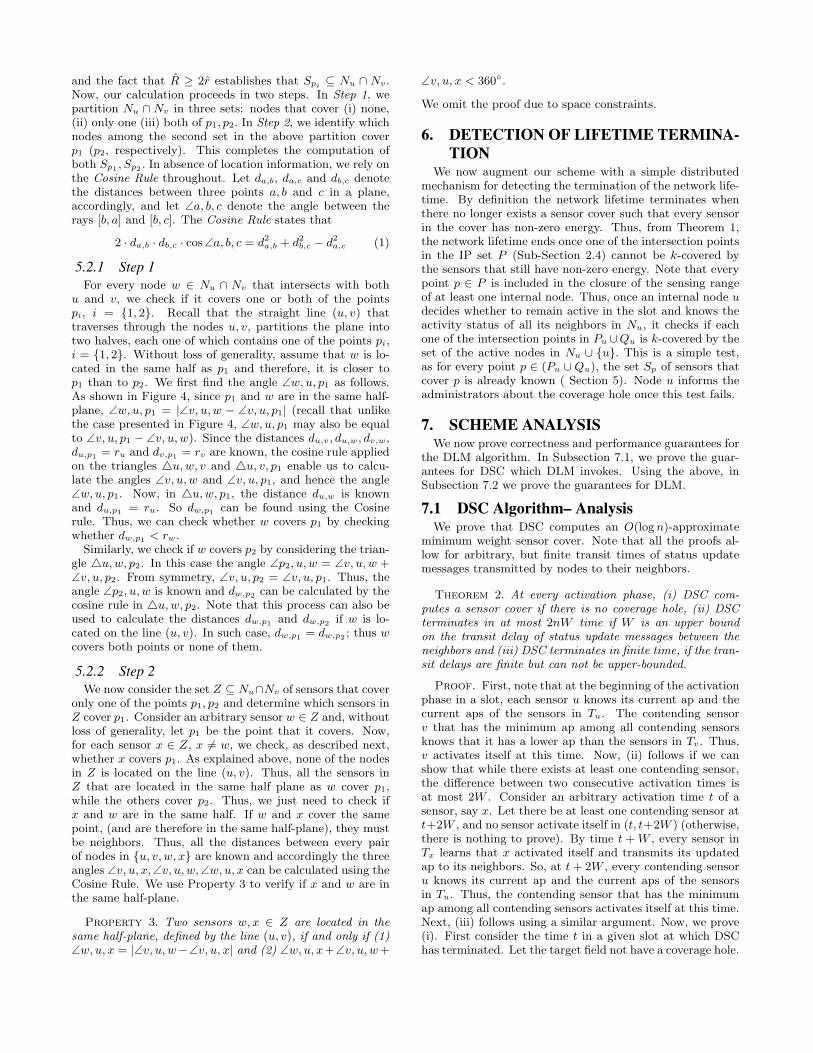
and the fact that R ≥ 2r establishes that Spi ⊆ Nu ∩ Nv.Now, our calculation proceeds in two steps. In Step 1, wepartition Nu ∩ Nv in three sets: nodes that cover (i) none,(ii) only one (iii) both of p1, p2. In Step 2, we identify whichnodes among the second set in the above partition coverp1 (p2, respectively). This completes the computation ofboth Sp1 , Sp2 . In absence of location information, we rely onthe Cosine Rule throughout. Let da,b, da,c and db,c denotethe distances between three points a, b and c in a plane,accordingly, and let ∠a, b, c denote the angle between therays [b, a] and [b, c]. The Cosine Rule states that
2 · da,b · db,c · cos ∠a, b, c = d2a,b + d2
b,c − d2a,c (1)
5.2.1 Step 1For every node w ∈ Nu ∩ Nv that intersects with both
u and v, we check if it covers one or both of the pointspi, i = {1, 2}. Recall that the straight line (u, v) thattraverses through the nodes u, v, partitions the plane intotwo halves, each one of which contains one of the points pi,i = {1, 2}. Without loss of generality, assume that w is lo-cated in the same half as p1 and therefore, it is closer top1 than to p2. We first find the angle ∠w, u, p1 as follows.As shown in Figure 4, since p1 and w are in the same half-plane, ∠w, u, p1 = |∠v, u, w − ∠v, u, p1| (recall that unlikethe case presented in Figure 4, ∠w, u, p1 may also be equalto ∠v, u, p1 − ∠v, u, w). Since the distances du,v, du,w, dv,w,du,p1 = ru and dv,p1 = rv are known, the cosine rule appliedon the triangles 4u, w, v and 4u, v, p1 enable us to calcu-late the angles ∠v, u, w and ∠v, u, p1, and hence the angle∠w, u, p1. Now, in 4u, w, p1, the distance du,w is knownand du,p1 = ru. So dw,p1 can be found using the Cosinerule. Thus, we can check whether w covers p1 by checkingwhether dw,p1 < rw.
Similarly, we check if w covers p2 by considering the trian-gle 4u, w, p2. In this case the angle ∠p2, u, w = ∠v, u, w +∠v, u, p2. From symmetry, ∠v, u, p2 = ∠v, u, p1. Thus, theangle ∠p2, u, w is known and dw,p2 can be calculated by thecosine rule in 4u, w, p2. Note that this process can also beused to calculate the distances dw,p1 and dw,p2 if w is lo-cated on the line (u, v). In such case, dw,p1 = dw,p2 ; thus wcovers both points or none of them.
5.2.2 Step 2We now consider the set Z ⊆ Nu∩Nv of sensors that cover
only one of the points p1, p2 and determine which sensors inZ cover p1. Consider an arbitrary sensor w ∈ Z and, withoutloss of generality, let p1 be the point that it covers. Now,for each sensor x ∈ Z, x 6= w, we check, as described next,whether x covers p1. As explained above, none of the nodesin Z is located on the line (u, v). Thus, all the sensors inZ that are located in the same half plane as w cover p1,while the others cover p2. Thus, we just need to check ifx and w are in the same half. If w and x cover the samepoint, (and are therefore in the same half-plane), they mustbe neighbors. Thus, all the distances between every pairof nodes in {u, v, w, x} are known and accordingly the threeangles ∠v, u, x, ∠v, u, w, ∠w, u, x can be calculated using theCosine Rule. We use Property 3 to verify if x and w are inthe same half-plane.
Property 3. Two sensors w, x ∈ Z are located in thesame half-plane, defined by the line (u, v), if and only if (1)∠w, u, x = |∠v, u, w−∠v, u, x| and (2) ∠w, u, x+∠v, u, w +
∠v, u, x < 360◦.
We omit the proof due to space constraints.
6. DETECTION OF LIFETIME TERMINA-TION
We now augment our scheme with a simple distributedmechanism for detecting the termination of the network life-time. By definition the network lifetime terminates whenthere no longer exists a sensor cover such that every sensorin the cover has non-zero energy. Thus, from Theorem 1,the network lifetime ends once one of the intersection pointsin the IP set P (Sub-Section 2.4) cannot be k-covered bythe sensors that still have non-zero energy. Note that everypoint p ∈ P is included in the closure of the sensing rangeof at least one internal node. Thus, once an internal node udecides whether to remain active in the slot and knows theactivity status of all its neighbors in Nu, it checks if eachone of the intersection points in Pu ∪Qu is k-covered by theset of the active nodes in Nu ∪ {u}. This is a simple test,as for every point p ∈ (Pu ∪Qu), the set Sp of sensors thatcover p is already known ( Section 5). Node u informs theadministrators about the coverage hole once this test fails.
7. SCHEME ANALYSISWe now prove correctness and performance guarantees for
the DLM algorithm. In Subsection 7.1, we prove the guar-antees for DSC which DLM invokes. Using the above, inSubsection 7.2 we prove the guarantees for DLM.
7.1 DSC Algorithm– AnalysisWe prove that DSC computes an O(log n)-approximate
minimum weight sensor cover. Note that all the proofs al-low for arbitrary, but finite transit times of status updatemessages transmitted by nodes to their neighbors.
Theorem 2. At every activation phase, (i) DSC com-putes a sensor cover if there is no coverage hole, (ii) DSCterminates in at most 2nW time if W is an upper boundon the transit delay of status update messages between theneighbors and (iii) DSC terminates in finite time, if the tran-sit delays are finite but can not be upper-bounded.
Proof. First, note that at the beginning of the activationphase in a slot, each sensor u knows its current ap and thecurrent aps of the sensors in Tu. The contending sensorv that has the minimum ap among all contending sensorsknows that it has a lower ap than the sensors in Tv. Thus,v activates itself at this time. Now, (ii) follows if we canshow that while there exists at least one contending sensor,the difference between two consecutive activation times isat most 2W . Consider an arbitrary activation time t of asensor, say x. Let there be at least one contending sensor att+2W , and no sensor activate itself in (t, t+2W ) (otherwise,there is nothing to prove). By time t + W , every sensor inTx learns that x activated itself and transmits its updatedap to its neighbors. So, at t + 2W , every contending sensoru knows its current ap and the current aps of the sensorsin Tu. Thus, the contending sensor that has the minimumap among all contending sensors activates itself at this time.Next, (iii) follows using a similar argument. Now, we prove(i). First consider the time t in a given slot at which DSChas terminated. Let the target field not have a coverage hole.
Then, each intersection point w in P is covered by k or morecontending sensors at the beginning of the activation phase.Since a contending sensor u decides to sleep only when all theintersection points in Pu are k-covered by activated sensors,all intersection points in P are k-covered by activated sensorsat t. The result follows by Theorem 1.
Now, recall that finding a minimum weight sensor cover isan instance of the minimum weight set cover problem. Wenow describe the well-known greedy Centralized Set Cover(CSC) algorithm that computes a O(log n)-approximate min-imum weight set cover [28]. At each iteration, it selects thesensor which has the lowest activation preference (ap) amongall the sensors, where ap is defined in the same way as forDSC, and then updates the ap’s of the unselected sensors.This process continues until the set of selected sensors con-stitutes a sensor cover.
Theorem 3. For a given setting and a set of weightsto the sensors, DSC and CSC select the same set of sen-sors. Thus, DSC obtains an O(log n)-approximate minimumweight sensor cover.
Proof. Let Y C = {v1, · · · , vmC} and Y D = {u1, · · · , umD}be the sets of selected sensors by CSC and DSC, respectively,sorted in increasing order according to their ap values at thetime that they were selected 4 (i.e., decided to stay active).Let vj and uj be the j-th sensors in Y C and Y D respec-tively, and let apC
j and apDj be their ap values. Moreover,
let Y Cj =
⋃i=1,j vj and Y D
j =⋃
i=1,j uj be the first j sen-
sors in sets Y C and Y D respectively. Not that the sensorsin Y C are arranged in the order in which they were selectedby CSC. However, the order on the sensors in Y D is notnecessarily the order in which they are activated by DSC.
Our proof utilizes the following properties:(1) During the execution of DSC, the ap of each node is anincreasing function of time.(2) Consider any node u ∈ Y D. Every sensor w ∈ Y D ∩ Tu
with lower ap value than u was selected before u by DSC.Similarly, any node w ∈ Y D ∩ Tu with higher ap value thanu was selected after node u by DSC.This property follows from property (1) and from the factthat under DSC, a sensor u becomes active only when (andif) it has lower ap value than its unselected neighbors in Tu.(3) The ap value of any node u during the execution of CSCand DSC is determined only by its already selected neighborsin Tu.(4) Suppose u ∈ Y D becomes active at time t1 under DSC.Then, for each w ∈ Y D ∩ Tu that became active before t1,u received an activation message from w before time t1.If this were not true for some w, then note that u would nothave activated itself at t1, since it would find its own ap tobe higher than that of w.
We seek to prove that Y C = Y D. Let Y C 6= Y D instead,and let j be the lowest index such that vj 6= uj . Initially,let us show by contradiction that j ≤ min(mC , mD). First,let mC > mD and j > mD. But, then, the first mD sensorsselected by CSC constitute a sensor cover and therefore CSCterminates after selecting at most the first mD sensors. Now,let mC < mD and j > mC (in particular j = mC + 1) andconsider the vicinity of the node uj . From Property (2),
4Here, by ap value of a node u ∈ Y D, we mean the latestap value calculated by u.
node uj was selected by DSC after every node in Y Dj−1 ∩
Tuj = Y DmC ∩ Tuj = Y C ∩ Tuj . However, since Y C is a
sensor cover, all intersection points in uj ’s sensing range arek-covered once DSC selects the nodes in Y C ∩ Tuj . Thus,DSC does not select uj after it has selected the sensors inY D
j−1 ∩ Tuj , and thus it does not select uj at all. Thus,
j ≤ min(mC , mD).We now show that apD
j ≥ apCj . If not, let apD
j < apCj
and consider the j-th iteration of CSC. The algorithm selectsas the j-th active sensor, the unselected sensor with minimalap value. Recall that at this stage uj has not been selectedby CSC. Since Y C
j−1 = Y Dj−1, from properties (2), (3) and
(4) above, it follows that at the j-th iteration of CSC theap value of node uj is the same as apD
j calculated by DSC.This is true since the ap value of node uj depends only onits selected neighbors in Y C
j−1 ∩Tuj = Y Dj−1 ∩Tuj , which
are the same sets 5 for both algorithms. Thus, CSC shouldselect node uj rather than node vj , which contradicts theassumption that apD
j < apCj . Thus apD
j ≥ apCj .
We next show that apDj ≤ apC
j . If not, apDj > apC
j .
Since vj is in Y C , it holds that nodes in Y Cj−1 do not cover
all the intersection points covered by the node vj . Thus,there are some nodes, denoted by set W , in the vicinityof vj , i.e., Pw ∩ Pvj 6= ∅ ∀w ∈ W , that were selected by
DSC and are not in Y Dj−1. First, assume that vj is the
first node in W selected by DSC. From Property (3) above,vj ’s ap value is determined only by the selected sensors inY D
j−1 = Y Cj−1. Thus, by Property (4), vj ’s ap value at the
time it is selected by DSC, is the same value as that at thetime it is selected by CSC, i.e., vj ’s ap value is apC
j , which
contradicts the assumption that apDj > apC
j . Thus, vj isnot the first node in W selected by DSC. Let x ∈ W , x 6= vj
be the first node in W selected by DSC and let apDx denote
its ap value at the time it was selected by DSC, say time tx.From our assumption, it follows that apD
x ≥ apDj > apC
j .Now, consider the ap value of node vj as calculated by DSCjust before time tx when node x is selected. Since x 6= vj
is the first node in W selected by DSC, just before time tx,the neighbors of vj selected by DSC must be from the setY D
j−1 (all the neighbors of vj need not be in Y Dj−1). From
Property (3), it holds that the ap value of vj is determinedonly by its selected neighbors. Thus, the ap value of vj justbefore time tx as calculated by DSC, denoted by apD
vj, is
at most apCj . Thus, apD
vj≤ apC
j < apDj ≤ apD
x. But,
then, vj should have been selected by DSC rather than nodex and its ap value should have been apD
vj, which contradicts
the assumption that apDj > apC
j .
Thus, apDj = apC
j . Hence, ID(uj) = ID(vj). Thus,uj = vj , which is a contradiction. The result follows.
7.2 DLM Algorithm– AnalysisWe now prove an approximation ratio for the lifetime at-
tained by the Distributed Lifetime Maximization (DLM) al-gorithm in Fig. 2. Our analysis is similar to the ones used byAspnes et al. [26] for online machine scheduling and virtualcircuit routing problems, and Awerbuch et. al [4], [5] for theonline virtual circuit routing problem.
Recall from Section 2.1 that a sensor that is active in a
5Note that by property (4), just before uj selected itselfunder DSC, it had updated its ap to account for the factthat all nodes in Y D
j−1 ∩ Tuj had activated themselves.
slot consumes 1 unit of energy and a sensor in sleep modeconsumes no energy. Throughout this section, all logarithmsare to the base 2. Finally, for proving the approximationratio, we additionally assume that the initial energy of eachsensor is large enough:
Assumption 1. Bu ≥ log µ, u ∈ S.
For simplicity, in the proof, we assume that Bu, u ∈ S areintegers. The proof can be easily extended to the case whenthey are real numbers.
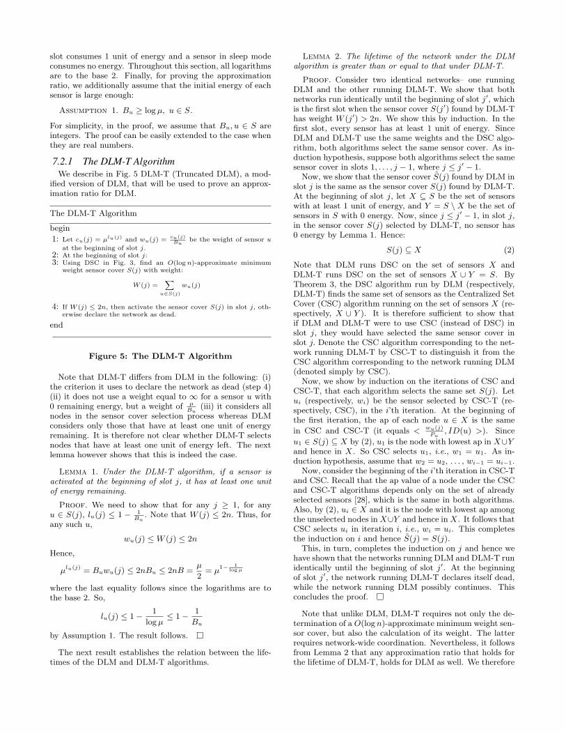
7.2.1 The DLM-T AlgorithmWe describe in Fig. 5 DLM-T (Truncated DLM), a mod-
ified version of DLM, that will be used to prove an approx-imation ratio for DLM.
The DLM-T Algorithm
begin
1: Let cu(j) = µlu(j) and wu(j) =cu(j)
Bube the weight of sensor u
at the beginning of slot j.2: At the beginning of slot j:3: Using DSC in Fig. 3, find an O(log n)-approximate minimum
weight sensor cover S(j) with weight:
W (j) =∑
u∈S(j)
wu(j)
4: If W (j) ≤ 2n, then activate the sensor cover S(j) in slot j, oth-erwise declare the network as dead.
end
Figure 5: The DLM-T Algorithm
Note that DLM-T differs from DLM in the following: (i)the criterion it uses to declare the network as dead (step 4)(ii) it does not use a weight equal to ∞ for a sensor u with0 remaining energy, but a weight of µ
Bu(iii) it considers all
nodes in the sensor cover selection process whereas DLMconsiders only those that have at least one unit of energyremaining. It is therefore not clear whether DLM-T selectsnodes that have at least one unit of energy left. The nextlemma however shows that this is indeed the case.
Lemma 1. Under the DLM-T algorithm, if a sensor isactivated at the beginning of slot j, it has at least one unitof energy remaining.
Proof. We need to show that for any j ≥ 1, for anyu ∈ S(j), lu(j) ≤ 1 − 1
Bu. Note that W (j) ≤ 2n. Thus, for
any such u,
wu(j) ≤ W (j) ≤ 2n
Hence,
µlu(j) = Buwu(j) ≤ 2nBu ≤ 2nB =µ
2= µ
1− 1log µ
where the last equality follows since the logarithms are tothe base 2. So,
lu(j) ≤ 1− 1
log µ≤ 1− 1
Bu
by Assumption 1. The result follows.
The next result establishes the relation between the life-times of the DLM and DLM-T algorithms.
Lemma 2. The lifetime of the network under the DLMalgorithm is greater than or equal to that under DLM-T.
Proof. Consider two identical networks– one runningDLM and the other running DLM-T. We show that bothnetworks run identically until the beginning of slot j′, whichis the first slot when the sensor cover S(j′) found by DLM-Thas weight W (j′) > 2n. We show this by induction. In thefirst slot, every sensor has at least 1 unit of energy. SinceDLM and DLM-T use the same weights and the DSC algo-rithm, both algorithms select the same sensor cover. As in-duction hypothesis, suppose both algorithms select the samesensor cover in slots 1, . . . , j − 1, where j ≤ j′ − 1.
Now, we show that the sensor cover S(j) found by DLM inslot j is the same as the sensor cover S(j) found by DLM-T.At the beginning of slot j, let X ⊆ S be the set of sensorswith at least 1 unit of energy, and Y = S \X be the set ofsensors in S with 0 energy. Now, since j ≤ j′ − 1, in slot j,in the sensor cover S(j) selected by DLM-T, no sensor has0 energy by Lemma 1. Hence:
S(j) ⊆ X (2)
Note that DLM runs DSC on the set of sensors X andDLM-T runs DSC on the set of sensors X ∪ Y = S. ByTheorem 3, the DSC algorithm run by DLM (respectively,DLM-T) finds the same set of sensors as the Centralized SetCover (CSC) algorithm running on the set of sensors X (re-spectively, X ∪ Y ). It is therefore sufficient to show thatif DLM and DLM-T were to use CSC (instead of DSC) inslot j, they would have selected the same sensor cover inslot j. Denote the CSC algorithm corresponding to the net-work running DLM-T by CSC-T to distinguish it from theCSC algorithm corresponding to the network running DLM(denoted simply by CSC).
Now, we show by induction on the iterations of CSC andCSC-T, that each algorithm selects the same set S(j). Letui (respectively, wi) be the sensor selected by CSC-T (re-spectively, CSC), in the i’th iteration. At the beginning ofthe first iteration, the ap of each node u ∈ X is the same
in CSC and CSC-T (it equals < wu(j)Pu
, ID(u) >). Since
u1 ∈ S(j) ⊆ X by (2), u1 is the node with lowest ap in X∪Yand hence in X. So CSC selects u1, i.e., w1 = u1. As in-duction hypothesis, assume that w2 = u2, . . . , wi−1 = ui−1.
Now, consider the beginning of the i’th iteration in CSC-Tand CSC. Recall that the ap value of a node under the CSCand CSC-T algorithms depends only on the set of alreadyselected sensors [28], which is the same in both algorithms.Also, by (2), ui ∈ X and it is the node with lowest ap amongthe unselected nodes in X∪Y and hence in X. It follows thatCSC selects ui in iteration i, i.e., wi = ui. This completesthe induction on i and hence S(j) = S(j).
This, in turn, completes the induction on j and hence wehave shown that the networks running DLM and DLM-T runidentically until the beginning of slot j′. At the beginningof slot j′, the network running DLM-T declares itself dead,while the network running DLM possibly continues. Thisconcludes the proof.
Note that unlike DLM, DLM-T requires not only the de-termination of a O(log n)-approximate minimum weight sen-sor cover, but also the calculation of its weight. The latterrequires network-wide coordination. Nevertheless, it followsfrom Lemma 2 that any approximation ratio that holds forthe lifetime of DLM-T, holds for DLM as well. We therefore
prove an approximation ratio for DLM, by proving one forDLM-T next.
7.2.2 Approximation RatioLet OPT be an optimal algorithm for the maximum life-
time problem, L be the network lifetime under the DLM-Talgorithm and L∗ be the network lifetime under OPT. Also,let L = {1, . . . , L} be the set of slots when the network isalive under the DLM-T algorithm and L∗ = {L+1, . . . , L∗}be the set of slots when the network is dead under the DLM-T algorithm, but alive under OPT.
We can view the situation after the network dies underDLM-T as if at the beginning of every slot j ∈ L∗, thenetwork finds an approximate minimum weight sensor cover(it finds the same sensor cover for each j ∈ L∗) and since theweight of this cover is greater than 2n, it does not activate it.Under DLM-T, no sensor is activated after slot L and hencethe weights of all sensors remain unchanged thereafter.
Let S(j) be the sensor cover found by DLM-T and S∗(j)be the sensor cover used by OPT in slot j. Also, let W (j)be the weight of S(j) and W ∗(j) be the sum of the weightsof the sensors in S∗(j) at the beginning of slot j when thenetwork is running DLM-T. We emphasize that the sensorcover S∗(j) is the one used by OPT in slot j, but the weightsof the sensors in W ∗(j) are those when the network is run-ning DLM-T.
Now, in every slot, the DLM-T algorithm finds an O(log n)-approximate minimum weight sensor cover. Hence, thereexists a constant α such that:
W (j) ≤ (α log n)W ∗(j) (3)
The following theorem proves the approximation ratio achievedby the DLM-T algorithm.
Theorem 4. L∗ is at most an O((log n)(log µ)) factorgreater than L.
The proof proceeds as follows. We first upper bound theamount by which the network lifetime under OPT can ex-ceed that under the DLM-T algorithm (Lemma 3). Next,we lower bound the lifetime achieved by DLM-T (Lemma 4).
Finally, we obtain an upper bound on the ratio L∗L
by com-bining the above bounds.
Lemma 3.
L∗ − L ≤ α log n
2n
∑u∈S
cu(L + 1) (4)
Proof. We define the indicator function:
I{u ∈ S∗(j)} =
{1 if u ∈ S∗(j)0 else
Since W (j) > 2n for j ∈ L∗, from (3) it follows that:
W ∗(j) ≥ 2n
α log n∀j ∈ L∗
Summing the above over j ∈ L∗, we get:
∑j∈L∗
W ∗(j) ≥ 2n
α log n(L∗ − L)
Hence,
2n
α log n(L∗ − L)
≤∑
j∈L∗
∑
u∈S∗(j)
1
Bucu(j)
=∑
j∈L∗
∑
u∈S∗(j)
1
Bucu(L + 1) (5)
=∑
j∈L∗
∑u∈S
cu(L + 1)
BuI{u ∈ S∗(j)}
=∑u∈S
cu(L + 1)
[1
Bu
∑j∈L∗
I{u ∈ S∗(j)}]
=∑u∈S
cu(L + 1) (6)
where in (5), we used the fact that since the network isdead under DLM-T at the beginning of slot L + 1, theenergy of each sensor remains same thereafter and hencecu(j) = cu(L + 1) ∀j ∈ L∗. We get (6) from the fact that∑
j∈L∗ I{u ∈ S∗(j)} is the number of slots in L∗ in whichsensor u is activated under OPT and must not exceed theinitial energy Bu of the sensor.
Lemma 4. ∑u∈S
cu(L + 1) ≤ n(2L log µ + 1) (7)
Proof. We begin by upper bounding the total growth inthe functions cu(.) of sensors u ∈ S(j) over slot j. For slotj ∈ L, we have:
∑
u∈S(j)
(cu(j + 1)− cu(j)) =∑
u∈S(j)
(µlu(j)+ 1
Bu − µlu(j))
=∑
u∈S(j)
µlu(j)(2log µBu − 1)
≤∑
u∈S(j)
µlu(j)
(log µ
Bu
)(8)
= log µ∑
u∈S(j)
µlu(j)
Bu
≤ 2n log µ (9)
where (8) results from the facts that log µBu
≤ 1 by Assump-
tion 1 and 2x − 1 ≤ x ∀x ∈ [0, 1]. Inequality (9) followsfrom:
∑
u∈S(j)
µlu(j)
Bu≤ 2n
which is true because the network is not declared dead byDLM-T at the beginning of slot j.
Now, in slot j, the energy of sensors u /∈ S(j) does notchange and hence cu(j + 1) = cu(j) ∀u /∈ S(j). So we get:
∑u∈S
(cu(j + 1)− cu(j)) =∑
u∈S(j)
(cu(j + 1)− cu(j))
≤ 2n log µ
Summing this inequality over j ∈ L:
L∑j=1
∑u∈S
(cu(j + 1)− cu(j)) ≤ 2nL log µ
The left hand side is a telescoping sum. So we get:∑u∈S
cu(L + 1) ≤ 2nL log µ +∑u∈S
cu(1)
But cu(1) = µ0 = 1 ∀u ∈ S. Thus,∑u∈S
cu(L + 1) ≤ n(2L log µ + 1)
Proof of Theorem 4. By Lemmas 3 and 4:
L∗ ≤ L(α(log n)(log µ) + 1) +α log n
2
The result follows since α is a constant.
8. SIMULATIONSWe now evaluate the performance of DLM using simula-
tions. We consider a WSN with n sensors, each with aninitial energy of B units, sensing and transmission radii of10 and 22 units respectively, deployed uniformly at randomin a 50 × 50 units2 target field, and examine the lifetimeattained by DLM as functions of n and B. Each time slotwas 1 unit long.
We compared the lifetimes of the network under three al-gorithms: the DLM algorithm (Fig. 2), the Garg-Konemann(GK) algorithm [11] and a heuristic proposed in [13, 21]that we denote by Min-Num. At every slot, Min-Num findsa sensor cover with the minimum number of nodes (up toan O(log n) factor) and activates it. GK [11] generatesa sequence of sets of weights to assign to the sensors andfinds minimum weight sensor covers for each set of weights.When the initial energy of each sensor is the same, each sen-sor cover selected by GK is activated for an equal amountof time, which is a monotonically increasing function of aninput parameter ε. Thus, the number of sensor cover com-putations per slot, and hence the computation time requiredfor GK, increases as ε decreases. The lifetime approxima-tion ratio guaranteed for the GK algorithm however worsenswith increase in ε 6.
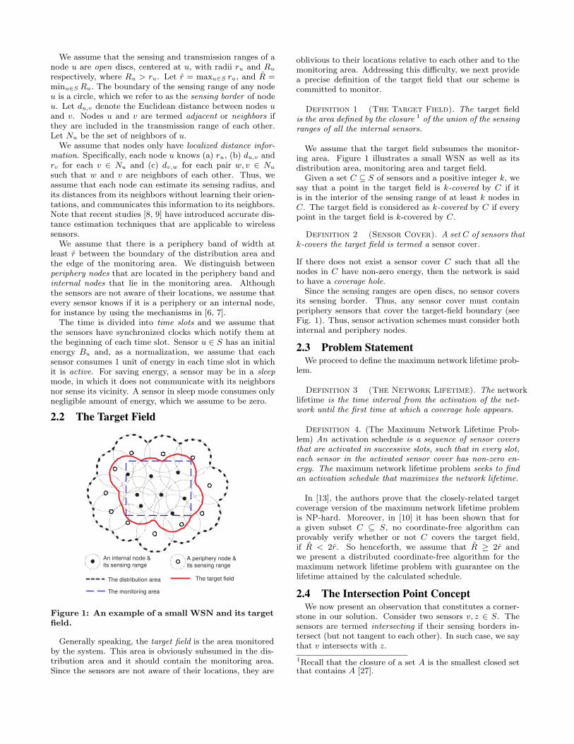
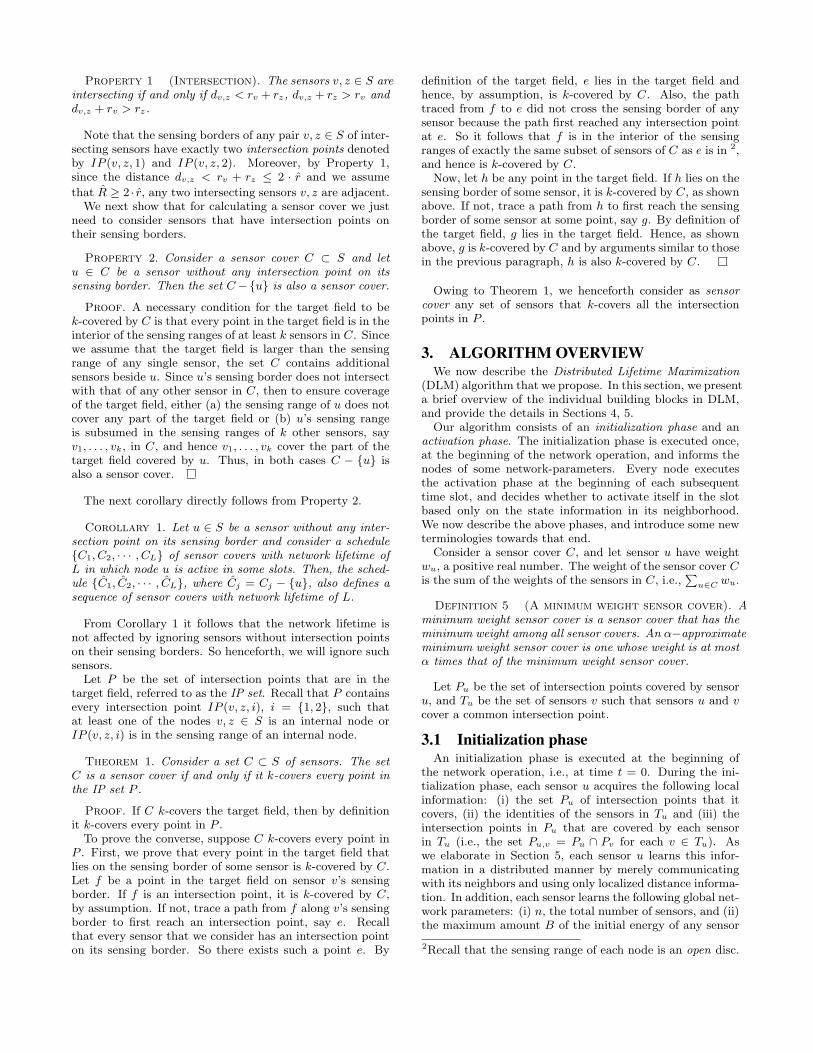
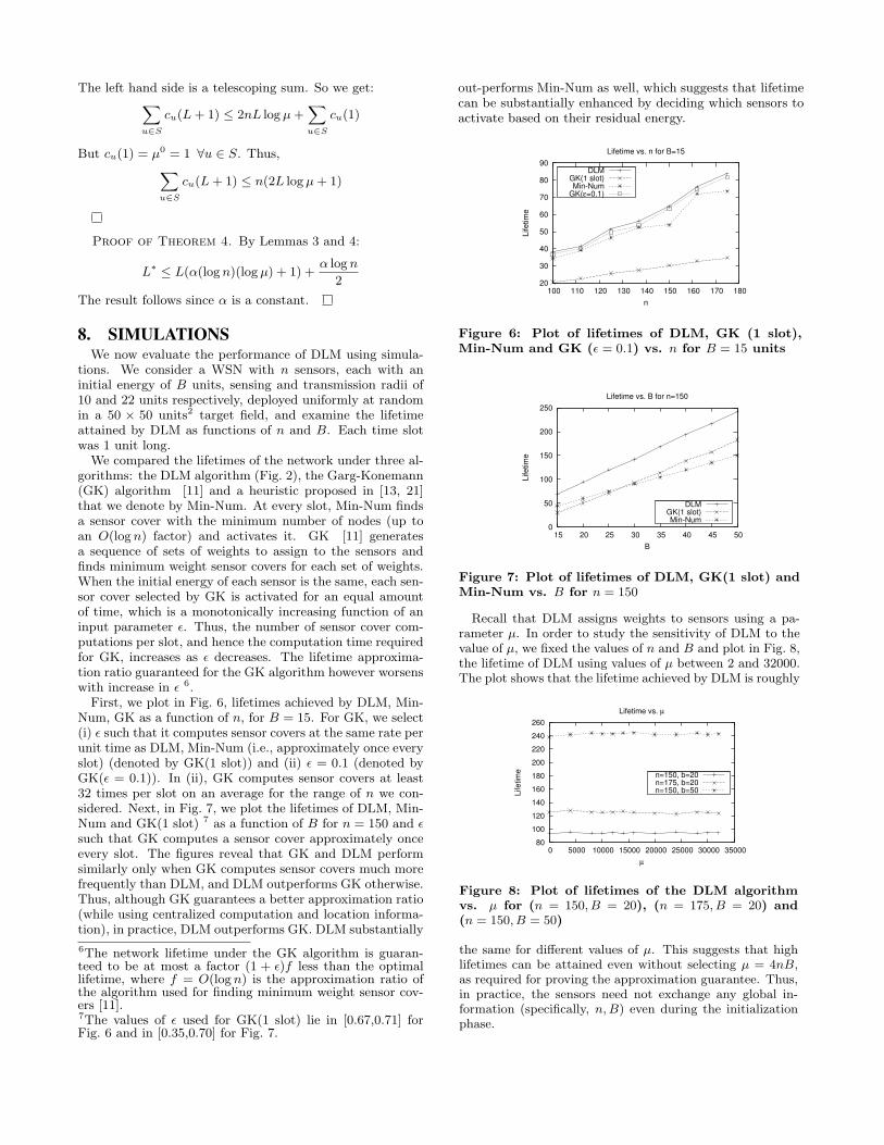
First, we plot in Fig. 6, lifetimes achieved by DLM, Min-Num, GK as a function of n, for B = 15. For GK, we select(i) ε such that it computes sensor covers at the same rate perunit time as DLM, Min-Num (i.e., approximately once everyslot) (denoted by GK(1 slot)) and (ii) ε = 0.1 (denoted byGK(ε = 0.1)). In (ii), GK computes sensor covers at least32 times per slot on an average for the range of n we con-sidered. Next, in Fig. 7, we plot the lifetimes of DLM, Min-Num and GK(1 slot) 7 as a function of B for n = 150 and εsuch that GK computes a sensor cover approximately onceevery slot. The figures reveal that GK and DLM performsimilarly only when GK computes sensor covers much morefrequently than DLM, and DLM outperforms GK otherwise.Thus, although GK guarantees a better approximation ratio(while using centralized computation and location informa-tion), in practice, DLM outperforms GK. DLM substantially
6The network lifetime under the GK algorithm is guaran-teed to be at most a factor (1 + ε)f less than the optimallifetime, where f = O(log n) is the approximation ratio ofthe algorithm used for finding minimum weight sensor cov-ers [11].7The values of ε used for GK(1 slot) lie in [0.67,0.71] forFig. 6 and in [0.35,0.70] for Fig. 7.
out-performs Min-Num as well, which suggests that lifetimecan be substantially enhanced by deciding which sensors toactivate based on their residual energy.
20
30
40
50
60
70
80
90
100 110 120 130 140 150 160 170 180
Lifetim
e
n
Lifetime vs. n for B=15
DLMGK(1 slot)Min-Num
GK(ε=0.1)
Figure 6: Plot of lifetimes of DLM, GK (1 slot),Min-Num and GK (ε = 0.1) vs. n for B = 15 units
0
50
100
150
200
250
15 20 25 30 35 40 45 50
Lifetim
e
B
Lifetime vs. B for n=150
DLMGK(1 slot)Min-Num
Figure 7: Plot of lifetimes of DLM, GK(1 slot) andMin-Num vs. B for n = 150
Recall that DLM assigns weights to sensors using a pa-rameter µ. In order to study the sensitivity of DLM to thevalue of µ, we fixed the values of n and B and plot in Fig. 8,the lifetime of DLM using values of µ between 2 and 32000.The plot shows that the lifetime achieved by DLM is roughly
80
100
120
140
160
180
200
220
240
260
0 5000 10000 15000 20000 25000 30000 35000
Lifetim
e
µ
Lifetime vs. µ
n=150, b=20n=175, b=20n=150, b=50
Figure 8: Plot of lifetimes of the DLM algorithmvs. µ for (n = 150, B = 20), (n = 175, B = 20) and(n = 150, B = 50)
the same for different values of µ. This suggests that highlifetimes can be attained even without selecting µ = 4nB,as required for proving the approximation guarantee. Thus,in practice, the sensors need not exchange any global in-formation (specifically, n, B) even during the initializationphase.
9. CONCLUSIONWe designed a distributed, coordinate-free algorithm for
attaining high lifetimes in sensor networks, subject to en-suring the k-coverage of the target field during the networklifetime. We proved that the lifetime attained by our algo-rithm approximates the maximum possible lifetime within alogarithmic approximation factor. Simulation results revealthat our algorithm substantially outperforms other schemesfor lifetime maximization.
10. ACKNOWLEDGMENTSThe contributions of G. Kasbekar and S. Sarkar have been
supported by NSF grants NCR-0238340, CNS-0721308, ECS-0622176.
11. REFERENCES[1] D. Subhadrabandhu, F. Anjum, S. Kannan, S. Sarkar
“Domination and Coverage Guarantees ThroughDistributed Computation” in Proceedings of 43dAnnual Allerton Conference on Communication,Control and Computing, Allerton, Monticello, Illinois,September 28-30, 2005
[2] C-F. Huang and Y.-C Tseng, “The Coverage Problemin a Wireless Sensor Network”, In Proc. of ACMWSNA’03, Sep. 2003.
[3] G. Kasbekar, Y. Bejerano and S. Sarkar, “GenericCoverage Verification without Location InformationUsing Dimension Reduction” in Proc. of Wiopt’09,Seoul, June 2009
[4] B. Awerbuch, Y. Azar, S. Plotkin“Throughput-Competitive On-Line Routing” inProceedings of IEEE Symposium on Foundations ofComputer Science, 1993.
[5] S. Leonardi “On-Line Network Routing” in OnlineAlgorithms- the State of the Art, ed. A. Fiat and G.Woeginger, 1998.
[6] C. Zhang, Y. Zhang and Y. Fang “Detecting CoverageBoundary Nodes in Wireless Sensor Networks”, InProc. of ICNSC ’06, April 2006.
[7] Y. Wang, J. Gao, J. S. B. Mitchell, “BoundaryRecognition in Sensor Networks by TopologicalMethods”, In Proc. of Mobicom ’06, Sep. 2006.
[8] B. Alavi and K. Pahlavan “Modeling of the TOA-basedDistance Measurement Error Using UWB IndoorRadio Measurements”, In IEEE CommunicationsLetters, Vol. 10, No. 4, April 2006, pp. 275-277.
[9] C. Y. Wen, R. D. Morris, and W. A. Sethares,“Distance Estimation Using BidirectionalCommunications Without Synchronous Clocking”,Accepted for publication in IEEE Trans. SignalProcessing.
[10] Y. Bejerano, “Simple and Efficient k-CoverageVerification without Location Information”. In Proc.of Infocom’08, Phoenix, Arizona, U.S.A., April 2008.
[11] P. Berman, G. Calinescu, C. Shah and A. Zelikovsly.“Efficient energy management in sensor networks”. InY. Xiao & Y. Pan (Eds.), Ad hoc and sensornetworks. Nova Science, 2005.
[12] F. Zhao and L. Guibas, “Wireless Sensor Networks:An Information Processing Approach”. MorganKaufmann, 2004.
[13] M. Cardei, M.T. Thai, Y. Li, W. Wu “Energy-EfficientTarget Coverage in Wireless Sensor Networks”. InProc. of Infocom’05, Miami, U.S.A., March 2005.
[14] M. Cardei and J. Wu. “Coverage in Wireless SensorNetworks”, Handbook of Sensor Networks. CRC Press2004.
[15] L. Wang and Y. Xiao “A Survey of Energy-EfficientScheduling Mechanisms in Sensor Networks” In MobileNetworks and Applications, Vol. 11, pp. 723-740,2006.
[16] R. R. Choudhury and R. Kravets,“Location-Independent Coverage in Wireless SensorNetworks”, Technical Report, UIUC, 2004
[17] R. Ghrist, A. Muhammad, “Coverage andhole-detection in sensor networks via homology”. InProc. of IPSN 2005, April 2005.
[18] A. Man-Cho So and Y. Ye. “On Solving CoverageProblems in a Wireless Sensor Network Using VoronoiDiagrams”. In Proc. of WINE 2005, LNCS 3828, pp.584-593, 2005.
[19] S. Meguerdichian, F. Koushanfar, M. Potkonjak, M.B. Srivastava, “Coverage Problems in Wireless Ad-hocSensor Networks”. In Proc. of Infocom’01, Anchorage,Alaska, U.S.A., April 2001.
[20] H. Zhang and J. C. Hou, “Maintaining sensingcoverage and connectivity in large sensor networks”. InInternational Journal of Wireless Ad Hoc and SensorNetworks, vol. 1, num. 1-2, pp. 89-123, January 2005.
[21] X. Wang, G. Xing, Y. Zhang, C. Lu, R. Pless, and C.Gill. “Integrated coverage and connectivityconfiguration in wireless sensor networks”. In Proc. ofACM SenSys’03, Los Angeles, CA, Nov. 2003.
[22] Y. Wu, S. Fahmy, N. Shroff, “On the Construction of aMaximum-Lifetime Data Gathering Tree in SensorNetworks: NP-Completeness and ApproximationAlgorithm” In Proc. of Infocom’08, Phoenix, Arizona,U.S.A., April 2008.
[23] D. Niculescu, “Positioning in ad hoc sensor networks”,In IEEE Network, Volume 18, Issue 4, July-Aug. 2004,pp. 24-29
[24] N. Patwari, J. N. Ash, S. Kyperountas, A. O. Hero,R.L. Moses and N. S. Correal, “Locating the nodes:cooperative localization in wireless sensor networks”,In IEEE Signal Processing Magazine, Volume 22, Issue4, July 2005 pp. 54-69
[25] Q. Shi, S. Kyperountas, N. S. Correal and F. Niu.“Performance Analysis of Relative LocationEstimation for Multihop Wireless Sensor Networks”.IEEE Journal On Selected Areas In Communications(JSAC), Vol 23, No. 4, April 2005.
[26] J. Aspnes, Y. Azar, A. Fiat, S. Plotkin, andO. Waarts. “On-line load balancing with applicationsto machine scheduling and virtual circuit routing”. InProc. ACM STOC, pp. 623–631, 1993.
[27] W. Rudin, “Principles of Mathematical Analysis”,Mc-Graw Hill, Third Edition, 1976.
[28] V. Chvatal, “A Greedy Heuristic for the Set-CoveringProblem”, Mathematics of Operations Research, Vol.4, No. 3 (Aug., 1979), pp. 233-235.