DI

SC

US

SI

ON

P

AP

ER

S

ER

IE

S

Forschungsinstitut zur Zukunft der ArbeitInstitute for the Study of Labor

Life Satisfaction and Relative Income:Perceptions and Evidence

IZA DP No. 4390

September 2009

Guy MayrazGert G. WagnerJürgen Schupp

Life Satisfaction and Relative Income:

Perceptions and Evidence

Guy Mayraz CEP, London School of Economics

Gert G. Wagner

SOEP, DIW Berlin, Max Planck Institute for Human Development and IZA

Jürgen Schupp

SOEP, DIW Berlin, Free University of Berlin and IZA

Discussion Paper No. 4390 September 2009

IZA

P.O. Box 7240 53072 Bonn

Germany

Phone: +49-228-3894-0 Fax: +49-228-3894-180

E-mail: iza@iza.org

Any opinions expressed here are those of the author(s) and not those of IZA. Research published in this series may include views on policy, but the institute itself takes no institutional policy positions. The Institute for the Study of Labor (IZA) in Bonn is a local and virtual international research center and a place of communication between science, politics and business. IZA is an independent nonprofit organization supported by Deutsche Post Foundation. The center is associated with the University of Bonn and offers a stimulating research environment through its international network, workshops and conferences, data service, project support, research visits and doctoral program. IZA engages in (i) original and internationally competitive research in all fields of labor economics, (ii) development of policy concepts, and (iii) dissemination of research results and concepts to the interested public. IZA Discussion Papers often represent preliminary work and are circulated to encourage discussion. Citation of such a paper should account for its provisional character. A revised version may be available directly from the author.

IZA Discussion Paper No. 4390 September 2009

ABSTRACT

Life Satisfaction and Relative Income: Perceptions and Evidence

Using a unique dataset we study both the actual and self-perceived relationship between subjective well-being and income comparisons against a wide range of potential comparison groups, enabling us to investigate a broader range of questions than in previous studies. In questions inserted into a 2008 module of the German-Socio Economic Panel Study we ask subjects to report (a) how their income compares to various groups, such a co-workers, friends, and neighbours, and (b) how important these income comparisons are to them. We find substantial gender differences, with income comparisons being much better predictors of subjective well-being in men than in women. Generic (same-gender) comparisons are the most important, followed by within profession comparisons. Once generic and within-profession comparisons are controlled for, income relative to neighbours has a negative coefficient, implying that living in a high-income neighbourhood increases happiness. The perceived importance of income comparisons is found to be uncorrelated with its actual relationship to subjective well-being, suggesting that people are unconscious of its real impact. Subjects who judge comparisons to be important are, however, significantly less happy than subjects who see income comparisons as unimportant. Finally, the marginal effect of relative income on subjective well-being does not depend on whether a subject is below or above the reference group income. JEL Classification: D31, D62, D63, I3, I31, Z13 Keywords: income comparisons, relative income, life satisfaction,

German Socio Economic Panel Study, SOEP Corresponding author: Guy Mayraz Centre for Economic Performance London School of Economics London WC2A 2AE United Kingdom E-mail: g.mayraz@lse.ac.uk

1 Introduction

Surveys of life satisfaction are increasingly used to study the relation-ship between subjective well-being and income. The essential questionis to what extent is it the case that higher income—or material well-being—translates into higher subjective well-being.

Early on it became apparent that different answers can be haddepending on how one asks the question. On the one hand, withina given country at a given point in time, the rich report higher lifesatisfaction than the poor (Frey and Stutzer, 2002). Moreover, as faras we can judge the subjective value of an extra dollar does decreasewith income, but never reaches zero. In fact, the value of a givenpercentage increase in income remains roughly the same whatever theincome level (Layard et al., 2008). On the other hand, Easterlin (1974)looked at the macro subjective well-being data, and found no time-series correlation between subjective well-being and GDP.

Easterlin’s findings (known as the Easterlin Paradox) raise the pos-sibility that, at least in developed countries, much of the subjectivevalue of higher income is due to relative comparisons. That is, therich are happier because they have more, rather than simply becausethey have a lot. Easterlin’s conclusions have been recently challengedby Stevenson and Wolfers (2008). This challenge only makes it moreimportant that we collect good evidence as to the effect relative com-parisons have on subjective well-being.

Focusing on income we want to understand what ceteris paribuseffect does a change in relative income have on a person’s subjectivewell-being. Consider the following regression model:

Hi = �+ �YRi + �′Yi +∑k

kXki + �i, (1)

where Hi is the life satisfaction reported by subject i, YRi is relativeincome, Yi absolute income, and Xk

i represent other controls. In prin-ciple, the ceteris paribus effect of relative income can be estimated bythe regression coefficient on YRi

.In practice, however, we are faced with the problem that we do

not observe YRi . To overcome this problem, the first thing researchersdo is to replace YRi by the reference income Y , that is the object ofcomparison. This step requires that the researcher commit to the pre-cise functional relationship between YRi

, Yi and Y . More substantialassumptions then have to be made as to what Y exactly is. Thereare many candidates: individuals may plausibly compare their incometo that of their friends, to that of co-workers, to other people in theirprofession, to their neighbours, or perhaps to other people of their agegroup, or some other still more general comparison group. We thushave Y1, Y2, Y3,etc.

2

Moreover, even if we decide to commit to one of these possibilities,further choices present themselves. Suppose we consider comparisonswith neighbours. Is it immediate neighbours? the whole street? theneighbourhood? the town? the entire region? Similarly, suppose weassume people compare their income to that of their co-workers. Thisstill leaves the question open whether they compare themselves witheveryone in their office, or perhaps with people doing a similar job only,or perhaps other workers who have similar experience or were hired ata similar time. Then, having committed to a functional form and aparticular well-defined sub-species of a reference group we are facedwith a final challenge: how to estimate the Y of our choice. This lastchallenge can also be significant. For example, in surveys generallyused for subjective well-being research we have no information on theearnings of friends or colleagues, and so cannot use the relevant Y ina regression.

In spite of all these challenges, researchers have forged ahead, fo-cusing on choices for Y that could be estimated from available data1.Clark et al. (2008) includes a detailed survey. By and large, publishedresults tend to show a negative estimated coefficient on Y , typicallycomparable to that on Yi, and thus consistent with a pure relative in-come effect (i.e. no effect for a change in absolute income that keepsrelative income constant). Nevertheless, results are often highly sensi-tive to specification, and in some cases the estimated coefficient is closeto zero, or even has the opposite sign. Interestingly, results may haveto do with the geographic scale of ‘neighbourhood’. For example, ina recent work that looked at neighbourhoods at the local street-blocklevel, Dittmann and Goebel (2009) find that life satisfaction increaseswhen a person has neighbours of a high socioeconomic status. Thisstudy is particularly relevant to our paper, since subjects reportingtheir income relative to that of their neighbours presumably have asimilarly local concept of neighbourhood in mind.

In this paper we propose to complement this literature by taking avery different approach. Instead of choosing a functional form, decid-ing on a particular reference group and subgroup, and then on someestimate of the chosen Y , we ask subjects to report YRi

directly. Specif-ically, we asked subjects to report on a scale their income relative tosome of the most plausible reference groups, including colleagues, sameprofession, same gender, same age, friends, and neighbours. We thusobserve six candidates for YRi , and can estimate regression models suchas that in Equation 1 directly. In particular, (1) we have values for

1The most common choices are the average income in the local area (i.e. some specialcase of the neighbours reference group), or the average income in a cell defined by somecombination of such variables as age, gender, and education, as in D’Ambrosio and Frick(2007).

3

YRiin relation to such groups as colleagues and friends, overcoming the

problem that the incomes of colleagues and friends are not observedin the survey data, and (2) these measures incorporate comparisonsagainst the particular colleagues, friends, neighbours etc. that subjectsperceive as relevant comparisons. This is important, since even if wehad observed the income of all colleagues, friends, and neighbours, itwould have required an additional difficult decision to identify the rel-evant individuals within those reference groups that should be used inestimating the reference group income.

In addition to asking subjects to report their relative income, weasked subjects to report how important they perceive each of thesecomparisons to be, allowing us to compare subjects’ own perceptionof the importance of income comparisons to its actual importance, asestimate by subjective well-being regressions. The survey we used forthese questions is the German Socio-Economic Panel Study (SOEP)2.Our questions were inserted into the pretest module of the 2008 wave,which consisted of 1,066 randomly chosen respondents.

Very little of the subjective well-being literature on relative com-parisons uses a similar approach to the one we take in this paper. Clarkand Senik (n.d.) report results using the third wave of the EuropeanSocial Survey, which included a question on the perceived importanceof relative income comparisons (but did not elicit YRi

, so the actualimportance cannot be tested). The results of Clark and Senik (n.d.)for the perceived importance of income are consistent with the relevantpart of our results. In a paper on rural migrants in China, Knight et al.(2008) asked subjects which group they are most likely to compare theirincome to, and found the subject’s own village was the most commonreference group for their subjects. McBride (2001) analysed a questionin the U.S. General Social Survey asking subjects to compare their liv-ing standards to those enjoyed by their parents when they were of asimilar age, and found that answers correlated strongly with reportedhappiness. Senik (forthcoming) studied post-transition countries, andinvestigated generic comparisons (“I have done better in life”) with thepeople a person used to know before transition started.

The reminder of the paper is organised as follows. Section 2 de-scribes the data. In Section 3 we report what comparisons subjectsperceive to be important, how important comparisons are perceivedto be, and what is the relationship between subjective well-being andperceiving comparisons to be important. In Section 4 we investigatethe actual importance of different relative income comparisons usinga regression model as in Equation 1 as the basic tool. In Section 5we compare perceived importance ratings with actual ratings, and alsoinvestigate whether the fact that a subject perceives comparisons to

2See Wagner et al. (2007) and http://www.diw.de/english/soep/soepoverview/27908.html.

4

be important is a good predictor of the actual relationship betweenthat subject’s subjective well-being and his or her relative income. InSection 6 we consider the possibility that YRi reports are biased bythe subject’s subjective well-being, and offer a test that suggests thisis not the case. In Section 7 we investigate whether, as some authorshave argued, the importance of relative comparisons is asymmetric,with the poor losing by relative comparisons more than the rich gain.In Section 8 we conclude.

2 The data

The data for this paper is the 2008 pretest module of the GermanSocio-Economic Panel Study (SOEP)3. SOEP is an annual householdpanel that has been conducted in Germany starting in 1984. The novelquestions we developed were inserted into the pretest module of the2008 wave. This sample for the pretest consisted of 1,066 randomlychosen respondents.

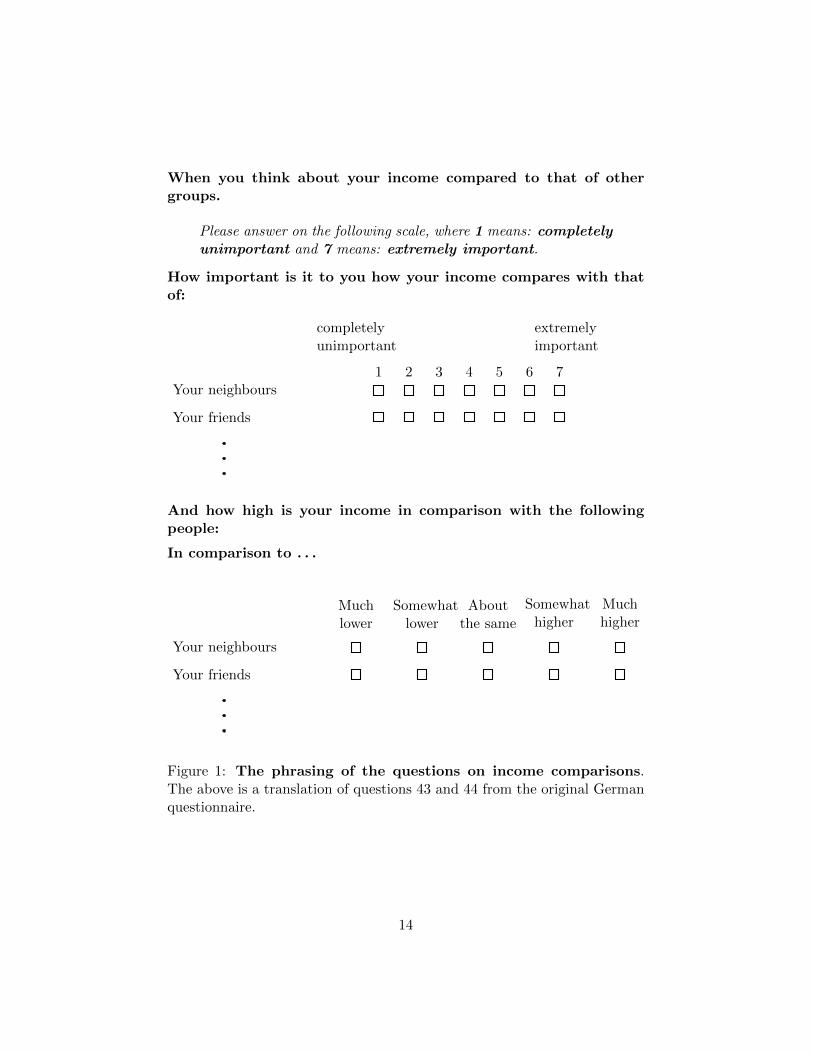
The first novel question we introduced asks respondents to reporthow important is it to them to compare their income against variousreference groups on a 1-7 scale, ranging from “completely unimpor-tant” to “extremely important”. The second question asks respondentsto report how their income compared with those groups on a 1-5 scaleranging from “much lower” to “much higher”. Figure 1 shows a trans-lation of the two questions. Descriptive statistics are in Table 1 andTable 2 respectively. The subjective well-being question we used isa standard life-satisfaction question, that is included in the commonSOEP questionnaire. The question asks: “How satisfied are you withyour life, all things considered?” with responses given on a 0-10 scale,in which 0 is labelled “completely dissatisfied” and 10 is labelled “com-pletely satisfied”. Other standard questions we used include gender,age, marital status, work status, and education level.

3 The subjective importance of income com-parisons

In this section we analyse responses to the question asking subjects toreport how important is it to them to compare their income againstvarious reference groups. Figure 1 shows a translation of the rele-vant question together with the question eliciting relative income (seeSection 4). Ratings were given on a scale of 1-7 ranging from “com-pletely unimportant” to “extremely important”. Descriptive statistics

3http://www.diw.de/english/soep/soepoverview/27908.html.

5

are reported in Table 1. The first thing to note is that about half thesubjects perceive relative income comparisons to be completely irrel-evant to their subjective well-being4. At the most extreme, compar-isons with neighbours (the original “keeping up with the Joneses”) arereported as completely unimportant by 2/3 of subjects. The compar-isons perceived as most important are work-related, with comparisonswith other people in the same profession appearing as most importantboth by average rating and by the percentage of people who perceivethe comparison to be at least somewhat important. There are no ap-parent differences in how men and women judge the importance ofincome comparisons.

There is a significant negative correlation between life satisfactionand the subjective importance of income comparisons. For example,one unit higher on the 1-7 scale of the subjective importance of com-paring income to other people of the same gender is associated withapproximately a 0.2 lower life satisfaction rating (measured on a 0-10scale). The third wave of the European Social Survey also has a ques-tion on the perceived importance of income comparisons. Clark andSenik (n.d.) report a similar negative correlation between life satisfac-tion and the subjective importance of income comparisons. Clark andSenik (n.d.) also report the results of a question that asked subjectsto choose which comparison they consider to be most important, andreport that work place comparisons are considered as most important,in agreement with the results reported here.

Ratings of perceived importance matter, in particular as people pre-sumably act on the basis of what they perceive as important. Theseratings cannot, however, tell us whether income comparisons actuallyare a significant determinant of subjective well-being, and which com-parisons really are important. To investigate these questions we nowleave the subjective ratings of perceived importance aside, and turn toregressions of life satisfaction on relative income and other controls. Ina later section we combine the two to investigate the information valueof perceived importance ratings.

4The third wave of the European Social Survey has a related question asking subjects“How important is it for you to compare your income with other peopleaAZs incomes?”.The distribution of replies reported in Clark and Senik (n.d.) is similar to the resultswe find in SOEP, with somewhat fewer subjects in the European Social Survey reportingincome comparisons to be completely unimportant, as compared with the SOEP results.The fact that the question in the European Social Survey combines all possible incomecomparisons may readily account for this difference.

6

4 The actual importance of relative incomecomparisons

In this section we investigate how important relative income compar-isons actually are, and which comparisons are the most important. Inthe key question we make use of, subjects were asked to report their in-come relative to various reference groups. Figure 1 shows a translationof this relevant question together with the question (discussed in theprevious section) eliciting the perceived importance of these compar-isons. Income relative to the different reference groups was reportedon a 1-5 scale ranging from “much lower” to “much higher”. Descrip-tive statistics are reported in Table 2. Reports were somewhat skewed,with the average male subject reporting income about 1/3 of a standarddeviation below the subjective comparison standard5. One possible ex-planation is that the subjective comparison standard is the mean of thereference group income, rather than its median. Given the skew in theincome distribution, the income of most subjects would then indeed bebelow the comparison standard.

In order to determine whether relative income can predict life satis-faction, life satisfaction was regressed separately on income relative tothe different reference groups. Regressions were run with and withoutabsolute income as a regressor (in log terms), and separately for menand women. The regression model with log income is

Hi = �+ �jYjRi

+ log Yi +∑k

�kXki + �i, (2)

where Hi is the life satisfaction reported by subject i, Y jRi

is subject i’sreported income relative to reference group j, Yi is subject i’s reportedincome in euros, and Xk

i represent other controls. Regressions withoutlog income omitted the log Yi regressor, but were otherwise the same.The results in Table 3 show a clear gender split: relative income hassignificant predictive power for men, but not for women. For example,income relative to other men has a standardised (beta) coefficient of0.25 for men when absolute income is not included in the regression,going down to 0.19 when income is included. For women the corre-sponding comparison with other women has standardised regressioncoefficients of only 0.06 and 0.02 respectively.

For women the small effect combined with the small sample sizemeans that none of the comparisons is statistically significant at the 5%level. It is therefore not really possible to rank the difference income

5In addition, females tend to rate their relative incomes as somewhat lower than domen. For example, the average man rates his income relative to other men as 2.82 on a1-5 scale, whereas the average woman rates her income relative to other women as 2.68on a 1-5 scale.

7

comparisons by importance. For men the effect size is much larger,and there is consequently also better statistical power. The resultsin Table 3 indicate that the important comparisons are work relatedcomparisons (same profession and with co-workers), and even more socomparisons with other men in general. Comparisons with friends andwith other individuals of the same age are less important. Finally,comparisons with neighbours are almost completely unimportant.

In addition to separate regressions we also regressed life satisfactionon relative income compared to all the reference groups in one regres-sion. The results in Table 4 are in line with the results of the separateregressions in that relative comparisons are much more significant formen than for women. Because of the small sample size and the corre-lation among YRi

with respect to different reference groups, the resultsare much less statistically significant. Nevertheless, it is clear that themost reference groups for men is the general one (all men) followedby same profession. Comparisons with neighbours are also somewhatimportant. Table 5 reports the results of a similar regression in whichonly these three relative income values were included. With fewer re-gressors the statistical significance goes up, with only a slight drop inthe regression R2. The implication of these results is that (a) the mostimportant income comparison is a generic one (“all men”), (b) thatwithin profession comparisons have an independent predictive power,and (c) that ceteris paribus people are happier if they live in a neigh-bourhood in which their neighbours are better off. These findings arediscussed in the Conclusion.

5 Comparing actual and perceived ratings

Table 3 tells how important relative income comparisons are to subjec-tive well-being, and which comparisons are most important. Compar-ing these results to the perceived ratings in Table 1 we see first thatthe gender split evident in Table 3 does not exist in the perceived rat-ings of Table 1. Both men and women perceive income comparisons asequally important, but the evidence suggests that only the subjectivewell-being of men is significantly correlated with such comparisons.

The comparisons of average ratings cannot, however, tell us whethera person’s estimate of the importance of relative income comparisons tohis or her happiness is a good predictor of its actual importance. Thissection presents a test of this possibility. The hypothesis to be tested isthat the reported perceived importance of relative income comparisonsis a good predictor of the correlation of relative income with subjectivewell-being. If this hypothesis is correct, we would expect the coefficienton YRi

in Equation 2 to vary depending on the perceived importance ofincome comparisons. To test this we expanded the model of Equation 2

8

to include the perceived importance of relative income comparisons,and an interaction term. The expanded model is thus

Hi = �+ �jYjRi

+ �′jI

jRi

+ +�′′j Y

jRiIjRi

+ log Yi +∑k

�kXki + �i, (3)

where Hi is the life satisfaction, Y jRi

is income relative to reference

group j, IjRiis the perceived importance of group j, Yi is income in

euros, and Xki represent other controls. Our focus is the estimate of

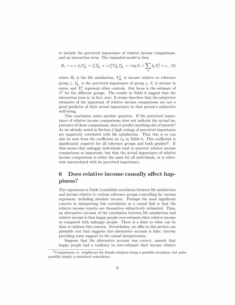
�′′ for the different groups. The results in Table 6 suggest that theinteraction term is, in fact, zero. It seems therefore that the subjectiveestimates of the important of relative income comparisons are not agood predictor of their actual importance to that person’s subjectivewell-being.

This conclusion raises another question. If the perceived impor-tance of relative income comparisons does not indicate the actual im-portance of those comparisons, does it predict anything else of interest?As we already noted in Section 3 high ratings of perceived importanceare negatively correlated with life satisfaction. That this is so canalso be seen from the coefficient on IR in Table 6. This coefficient issignificantly negative for all reference groups and both genders6. Itthus seems that unhappy individuals tend to perceive relative incomecomparisons as important, but that the actual importance of relativeincome comparisons is either the same for all individuals, or is other-wise uncorrelated with its perceived importance.

6 Does relative income causally affect hap-piness?

The regressions in Table 3 establish correlation between life satisfactionand income relative to various reference groups controlling for variousregressors, including absolute income. Perhaps the most significantconcern in interpreting this correlation as a causal link is that therelative income reports are themselves subjectively estimated. Thus,an alternative account of the correlation between life satisfaction andrelative income is that happy people over-estimate their relative incomeas compared with unhappy people. There is a limit to what can bedone to address this concern. Nevertheless, we offer in this section oneplausible test that suggests this alternative account is false, therebyproviding some support to the causal interpretation.

Suppose that the alternative account was correct, namely thathappy people had a tendency to over-estimate their income relative

6Comparisons vs. neighbours for female subjects being a possible exception, but quitepossibly simply a statistical coincidence.

9

to other people, presumably because higher relative income is desir-able. If that were the case then we would expect such a bias to begreater the more important relative income comparisons are perceivedto be. Because we observe the subjective importance of relative incomecomparisons this hypothesis is testable.

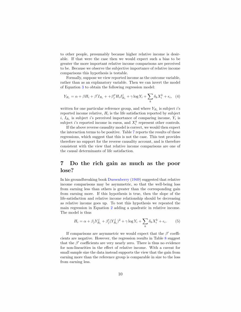
Formally, suppose we view reported income as the outcome variable,rather than as an explanatory variable. Then we can invert the modelof Equation 3 to obtain the following regression model:

YRi= �+ �Hi + �′IRi

+ +�′′jHiI

jRi

+ log Yi +∑k

�kXki + �i, (4)

written for one particular reference group, and where YRiis subject i’s

reported income relative, Hi is the life satisfaction reported by subjecti, IRi

is subject i’s perceived importance of comparing income, Yi issubject i’s reported income in euros, and Xk

i represent other controls.If the above reverse causality model is correct, we would then expect

the interaction terms to be positive. Table 7 reports the results of theseregressions, which suggest that this is not the case. This test providestherefore no support for the reverse causality account, and is thereforeconsistent with the view that relative income comparisons are one ofthe causal determinants of life satisfaction.

7 Do the rich gain as much as the poorlose?

In his groundbreaking book Duesenberry (1949) suggested that relativeincome comparisons may be asymmetric, so that the well-being lossfrom earning less than others is greater than the corresponding gainfrom earning more. If this hypothesis is true, then the slope of thelife-satisfaction and relative income relationship should be decreasingas relative income goes up. To test this hypothesis we repeated themain regression in Equation 2 adding a quadratic in relative income.The model is thus

Hi = �+ �jYjRi

+ �′j(Y

jRi

)2 + log Yi +∑k

�kXki + �i. (5)

If comparisons are asymmetric we would expect that the �′ coeffi-cients are negative. However, the regression results in Table 8 suggestthat the �′ coefficients are very nearly zero. There is thus no evidencefor non-linearities in the effect of relative income. With a caveat forsmall sample size the data instead supports the view that the gain fromearning more than the reference group is comparable in size to the lossfrom earning less.

10

8 Conclusion

In this paper we sought to study the relationship between life satisfac-tion and income relative to various reference group. The key to thisstudy has been special questions we inserted into the pretest moduleof the 2008 wave of the German Socio-Economic Panel Study (SOEP).Specifically, we asked subjects to evaluate how their income comparesto various reference groups, and also to evaluate the subjective impor-tance of how their income compares to these reference groups. Thesequestions enabled us to assess the actual importance of relative incomecomparisons vs. the different reference groups.

Our first finding is that the life satisfaction of men is significantlycorrelated with their relative income, but that this is not the case withwomen. Second, we are able to establish that individually the more im-portant comparisons are either generic (all men) or work-related, andthat comparisons with friends, other same-age individuals, and neigh-bours are considerably less important. Third, in a combined regressionwe find that almost all the effect of relative comparisons is captured bythe generic (all men) comparison, a within profession comparison, anda comparison with neighbours, where the coefficients on relative incomeare positive for the generic and profession comparisons and negative onthe comparison with neighbours. Fourth, we find that high perceivedimportance of income comparisons is correlated with lower subjectivewell-being, but does not predict how important to subjective well-beingrelative income actually is. Finally we find that the marginal impor-tance of relative income comparisons is the same whether income islower or higher than that of the reference group.

In line with previous studies our findings confirm the importance ofrelative income comparisons to subjective well-being. However, usingthe new data we find that the picture is significantly more complicatedthan first envisaged. In particular, (a) there appears to be a big genderdifference, with a much greater effect for male, (b) the most impor-tant comparison seems to be a generic one, rather than a comparisonwith close others. A possible explanation is that income comparisonsfirst and foremost proxy for the ability to purchase positional goods,the price of which is determined outside an immediate social environ-ment7, (c) within-profession comparisons are important independentlyof other income comparisons, suggesting that professional success isdesirable in itself, separately from its correlation with higher income,and (d) other things being equal, people seem to be happier if they

7Positional goods are such goods as a house by the lake, which are in inherently limitedsupply. Because of the limited supply, prices adjust so that positional goods can only everbe purchased by those with a high enough income relative to other consumers. Theeconomist Robert Frank has written extensively about positional goods (Frank, 1991,2001, 2005).

11

earn less than their neighbours. That this is the case suggests thatpeople significantly benefit from living in a good neighbourhood, andlose little—if anything—by the negative relative comparison8.

References

Clark, A., Frijters, P. and Shields, M. (2008). Relative Income, Hap-piness and Utility: An Explanation for the Easterlin Paradox andOther Puzzles, Journal of Economic Literature 46(1): 95–144.

Clark, A. and Senik, C. (n.d.). Who compares to whom? The anatomyof income comparisons in Europe.

D’Ambrosio, C. and Frick, J. (2007). Income satisfaction and rel-ative deprivation: An empirical link, Social Indicators Research81(3): 497–519.

Dittmann, J. and Goebel, J. (2009). Your house, your car, your ed-ucation The socioeconomic situation of the neighborhood and itsimpact on life satisfaction in Germany, Social Indicators Research83(forthcoming).

Duesenberry, J. (1949). Income, saving and the theory of consumerbehavior, Harvard University Press.

Easterlin, R. (1974). Does economic growth improve the human lot?some empirical evidence, in P. A. David and M. W. Reder (eds),Nations and Households in Economic Growth: Essays in Honor ofMoses Abramowitz, Academic Press, New-York, pp. 89–125.

Frank, R. (1991). Positional externalities, Strategy and Choice, MITPress, Cambridge, MA pp. 25–47.

Frank, R. (2001). Luxury fever: Why money fails to satisfy in an eraof excess, Simon and Schuster.

Frank, R. (2005). Positional externalities cause large and preventablewelfare losses, American Economic Review pp. 137–141.

8The ceteris paribus clause is important. As Table 3 shows, the coefficient is positiveif income comparison with neighbours is the only comparison included in the regression.Our results are thus consistent with those of researchers who include only income compar-isons with neighbours in a regression, and find the coefficient to be significantly positive(this result is more commonly reported as a negative coefficient on the mean income ofneighbours). Moreover, researchers who use local comparisons in studies of relative in-come typically define the locality as a much larger area than a local neighbourhood. Forexample, Luttmer (2005) uses units of about 100,000 people, which are perhaps closer tothe generic group in this paper.

12

Frey, B. and Stutzer, A. (2002). What Can Economists Learn fromHappiness Research?, Journal of Economic Literature 40(2): 402–435.

Knight, J., Song, L. and Gunatilaka, R. (2008). Subjective well-beingand its determinants in rural China, China Economic Review .

Layard, R., Mayraz, G. and Nickell, S. (2008). The marginal utility ofincome, Journal of Public Economics 92(8-9): 1846–1857.

Luttmer, E. F. (2005). Neighbours as negatives: Relative earnings andwell-being, Quarterly Journal of Economics 120(3): 963–1002.

McBride, M. (2001). Relative-income effects on subjective well-being inthe cross-section, Journal of Economic Behavior and Organization45(3): 251–278.

Senik, C. (forthcoming). Direct evidence on income comparisons andtheir welfare effects, Journal of Economic Behaviour and Organisa-tion .

Stevenson, B. and Wolfers, J. (2008). Economic Growth and SubjectiveWell-Being: Reassessing the Easterlin Paradox, Brookings Papers onEconomic Activity .

Wagner, G., Frick, J. and Schupp, J. (2007). The German socio-economic panel study (SOEP)–scope, evolution and enhancements,Schmollers Jahrbuch 127(1): 139–169.

13

When you think about your income compared to that of othergroups.

Please answer on the following scale, where 1 means: completelyunimportant and 7 means: extremely important.

How important is it to you how your income compares with thatof:

completelyunimportant

extremelyimportant

1 2 3 4 5 6 7Your neighbours

Your friends

And how high is your income in comparison with the followingpeople:

In comparison to . . .

Muchlower

Somewhatlower

Aboutthe same

Somewhathigher

Muchhigher

Your neighbours

Your friends

Figure 1: The phrasing of the questions on income comparisons.The above is a translation of questions 43 and 44 from the original Germanquestionnaire.

14

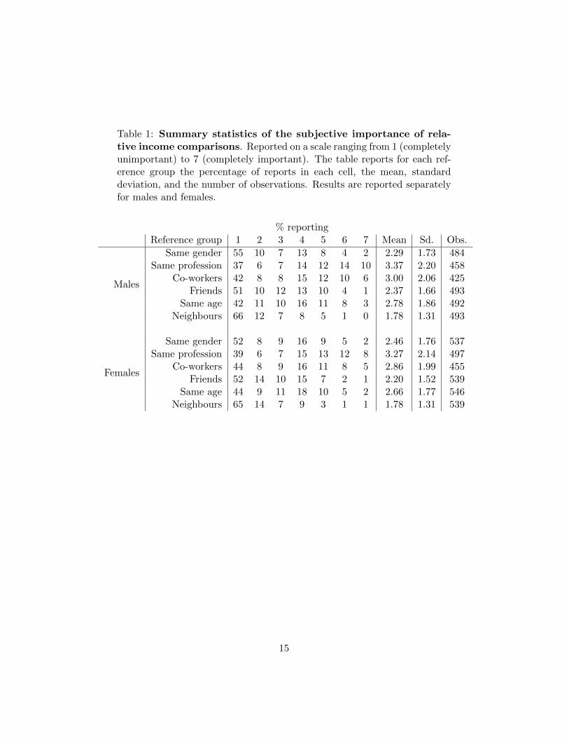
Table 1: Summary statistics of the subjective importance of rela-tive income comparisons. Reported on a scale ranging from 1 (completelyunimportant) to 7 (completely important). The table reports for each ref-erence group the percentage of reports in each cell, the mean, standarddeviation, and the number of observations. Results are reported separatelyfor males and females.

% reportingReference group 1 2 3 4 5 6 7 Mean Sd. Obs.

Males

Same gender 55 10 7 13 8 4 2 2.29 1.73 484Same profession 37 6 7 14 12 14 10 3.37 2.20 458

Co-workers 42 8 8 15 12 10 6 3.00 2.06 425Friends 51 10 12 13 10 4 1 2.37 1.66 493

Same age 42 11 10 16 11 8 3 2.78 1.86 492Neighbours 66 12 7 8 5 1 0 1.78 1.31 493

Females

Same gender 52 8 9 16 9 5 2 2.46 1.76 537Same profession 39 6 7 15 13 12 8 3.27 2.14 497

Co-workers 44 8 9 16 11 8 5 2.86 1.99 455Friends 52 14 10 15 7 2 1 2.20 1.52 539

Same age 44 9 11 18 10 5 2 2.66 1.77 546Neighbours 65 14 7 9 3 1 1 1.78 1.31 539

15

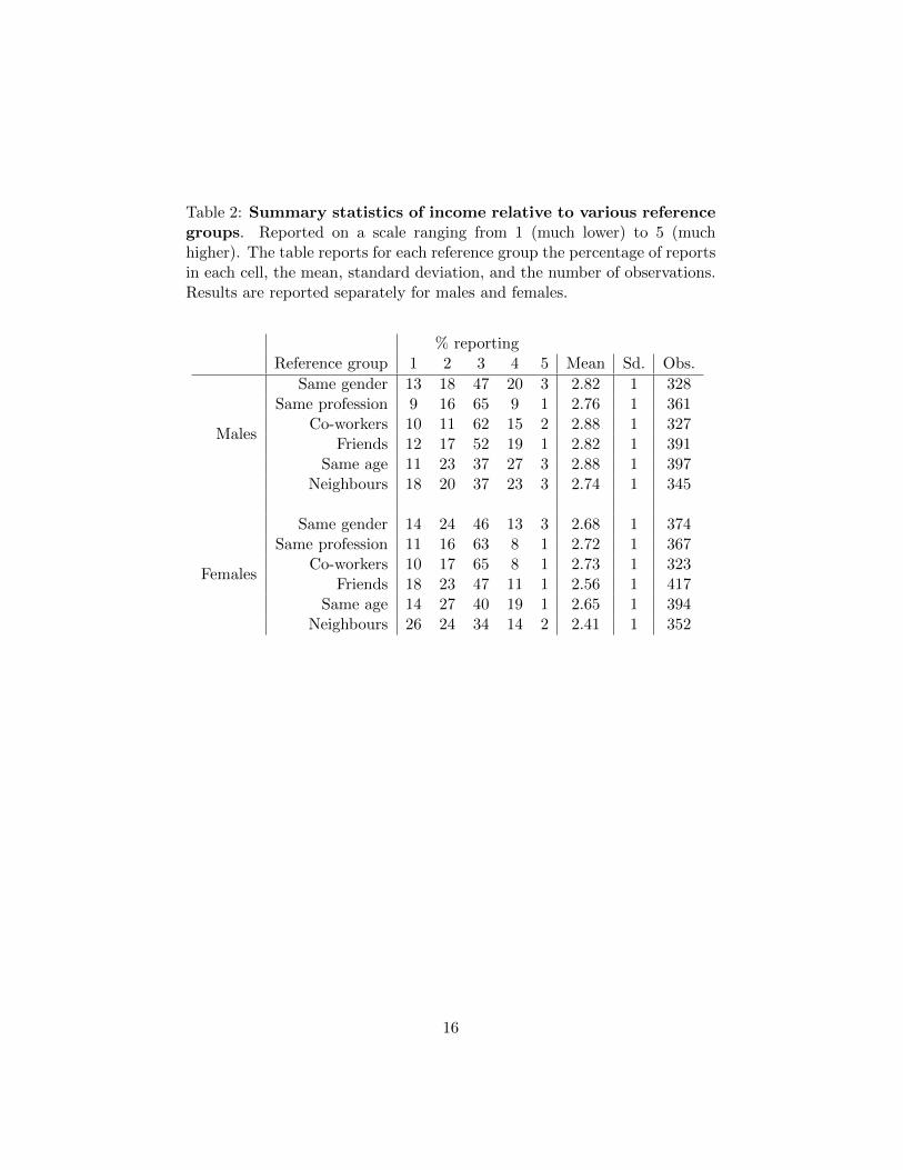
Table 2: Summary statistics of income relative to various referencegroups. Reported on a scale ranging from 1 (much lower) to 5 (muchhigher). The table reports for each reference group the percentage of reportsin each cell, the mean, standard deviation, and the number of observations.Results are reported separately for males and females.

% reportingReference group 1 2 3 4 5 Mean Sd. Obs.

Males

Same gender 13 18 47 20 3 2.82 1 328Same profession 9 16 65 9 1 2.76 1 361

Co-workers 10 11 62 15 2 2.88 1 327Friends 12 17 52 19 1 2.82 1 391

Same age 11 23 37 27 3 2.88 1 397Neighbours 18 20 37 23 3 2.74 1 345

Females

Same gender 14 24 46 13 3 2.68 1 374Same profession 11 16 63 8 1 2.72 1 367

Co-workers 10 17 65 8 1 2.73 1 323Friends 18 23 47 11 1 2.56 1 417

Same age 14 27 40 19 1 2.65 1 394Neighbours 26 24 34 14 2 2.41 1 352

16

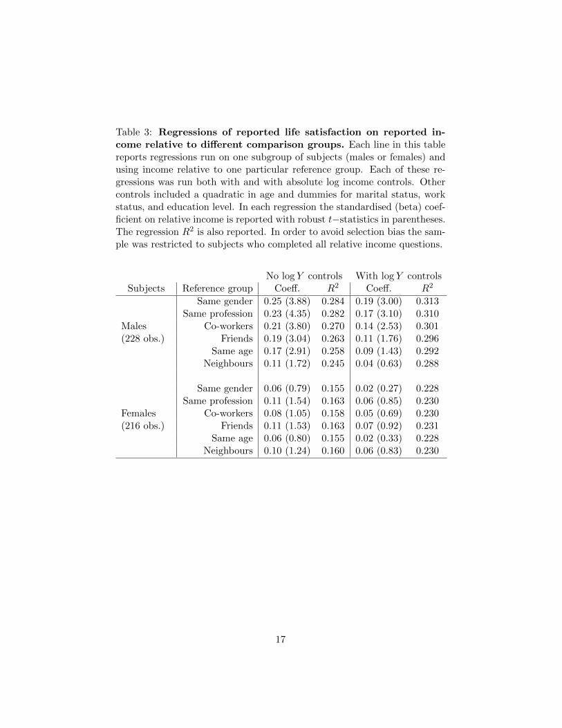
Table 3: Regressions of reported life satisfaction on reported in-come relative to different comparison groups. Each line in this tablereports regressions run on one subgroup of subjects (males or females) andusing income relative to one particular reference group. Each of these re-gressions was run both with and with absolute log income controls. Othercontrols included a quadratic in age and dummies for marital status, workstatus, and education level. In each regression the standardised (beta) coef-ficient on relative income is reported with robust t−statistics in parentheses.The regression R2 is also reported. In order to avoid selection bias the sam-ple was restricted to subjects who completed all relative income questions.

No log Y controls With log Y controlsSubjects Reference group Coeff. R2 Coeff. R2

Males(228 obs.)

Same gender 0.25 (3.88) 0.284 0.19 (3.00) 0.313Same profession 0.23 (4.35) 0.282 0.17 (3.10) 0.310

Co-workers 0.21 (3.80) 0.270 0.14 (2.53) 0.301Friends 0.19 (3.04) 0.263 0.11 (1.76) 0.296

Same age 0.17 (2.91) 0.258 0.09 (1.43) 0.292Neighbours 0.11 (1.72) 0.245 0.04 (0.63) 0.288

Females(216 obs.)

Same gender 0.06 (0.79) 0.155 0.02 (0.27) 0.228Same profession 0.11 (1.54) 0.163 0.06 (0.85) 0.230

Co-workers 0.08 (1.05) 0.158 0.05 (0.69) 0.230Friends 0.11 (1.53) 0.163 0.07 (0.92) 0.231

Same age 0.06 (0.80) 0.155 0.02 (0.33) 0.228Neighbours 0.10 (1.24) 0.160 0.06 (0.83) 0.230

17

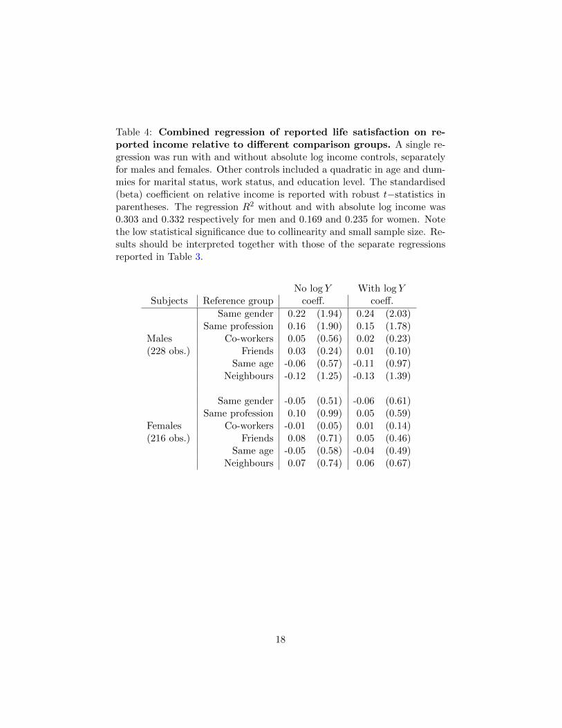
Table 4: Combined regression of reported life satisfaction on re-ported income relative to different comparison groups. A single re-gression was run with and without absolute log income controls, separatelyfor males and females. Other controls included a quadratic in age and dum-mies for marital status, work status, and education level. The standardised(beta) coefficient on relative income is reported with robust t−statistics inparentheses. The regression R2 without and with absolute log income was0.303 and 0.332 respectively for men and 0.169 and 0.235 for women. Notethe low statistical significance due to collinearity and small sample size. Re-sults should be interpreted together with those of the separate regressionsreported in Table 3.

No log Y With log YSubjects Reference group coeff. coeff.

Males(228 obs.)

Same gender 0.22 (1.94) 0.24 (2.03)Same profession 0.16 (1.90) 0.15 (1.78)

Co-workers 0.05 (0.56) 0.02 (0.23)Friends 0.03 (0.24) 0.01 (0.10)

Same age -0.06 (0.57) -0.11 (0.97)Neighbours -0.12 (1.25) -0.13 (1.39)

Females(216 obs.)

Same gender -0.05 (0.51) -0.06 (0.61)Same profession 0.10 (0.99) 0.05 (0.59)

Co-workers -0.01 (0.05) 0.01 (0.14)Friends 0.08 (0.71) 0.05 (0.46)

Same age -0.05 (0.58) -0.04 (0.49)Neighbours 0.07 (0.74) 0.06 (0.67)

18

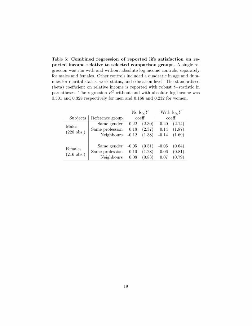
Table 5: Combined regression of reported life satisfaction on re-ported income relative to selected comparison groups. A single re-gression was run with and without absolute log income controls, separatelyfor males and females. Other controls included a quadratic in age and dum-mies for marital status, work status, and education level. The standardised(beta) coefficient on relative income is reported with robust t−statistic inparentheses. The regression R2 without and with absolute log income was0.301 and 0.328 respectively for men and 0.166 and 0.232 for women.

No log Y With log YSubjects Reference group coeff. coeff.

Males(228 obs.)

Same gender 0.22 (2.30) 0.20 (2.14)Same profession 0.18 (2.37) 0.14 (1.87)

Neighbours -0.12 (1.38) -0.14 (1.69)

Females(216 obs.)

Same gender -0.05 (0.51) -0.05 (0.64)Same profession 0.10 (1.28) 0.06 (0.81)

Neighbours 0.08 (0.88) 0.07 (0.79)

19

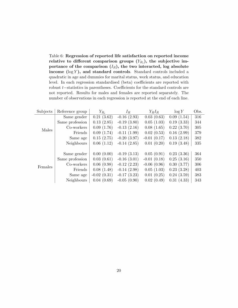
Table 6: Regression of reported life satisfaction on reported incomerelative to different comparison groups (YRi), the subjective im-portance of the comparison (IR), the two interacted, log absoluteincome (log Y ), and standard controls. Standard controls included aquadratic in age and dummies for marital status, work status, and educationlevel. In each regression standardised (beta) coefficients are reported withrobust t−statistics in parentheses. Coefficients for the standard controls arenot reported. Results for males and females are reported separately. Thenumber of observations in each regression is reported at the end of each line.

Subjects Reference group YRi IR YRIR log Y Obs.

Males

Same gender 0.21 (3.62) -0.16 (2.93) 0.03 (0.63) 0.09 (1.54) 316Same profession 0.13 (2.85) -0.19 (3.80) 0.05 (1.03) 0.19 (3.33) 344

Co-workers 0.09 (1.76) -0.13 (2.16) 0.08 (1.65) 0.22 (3.70) 305Friends 0.09 (1.74) -0.11 (1.99) 0.02 (0.53) 0.16 (2.99) 379

Same age 0.15 (2.75) -0.20 (3.97) -0.01 (0.17) 0.13 (2.18) 382Neighbours 0.06 (1.12) -0.14 (2.85) 0.01 (0.20) 0.19 (3.48) 335

Females

Same gender 0.00 (0.00) -0.19 (3.13) 0.05 (0.91) 0.23 (3.36) 364Same profession 0.03 (0.61) -0.16 (3.01) -0.01 (0.18) 0.25 (3.16) 350

Co-workers 0.06 (0.98) -0.12 (2.23) -0.06 (0.96) 0.30 (3.77) 306Friends 0.08 (1.48) -0.14 (2.98) 0.05 (1.03) 0.23 (3.28) 403

Same age -0.02 (0.31) -0.17 (3.23) 0.01 (0.25) 0.24 (3.59) 383Neighbours 0.04 (0.69) -0.05 (0.90) 0.02 (0.49) 0.31 (4.33) 343

20

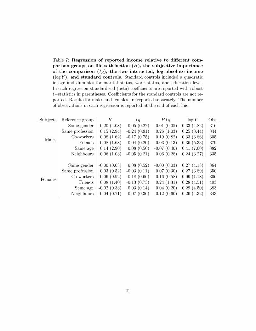
Table 7: Regression of reported income relative to different com-parison groups on life satisfaction (H), the subjective importanceof the comparison (IR), the two interacted, log absolute income(log Y ), and standard controls. Standard controls included a quadraticin age and dummies for marital status, work status, and education level.In each regression standardised (beta) coefficients are reported with robustt−statistics in parentheses. Coefficients for the standard controls are not re-ported. Results for males and females are reported separately. The numberof observations in each regression is reported at the end of each line.

Subjects Reference group H IR HIR log Y Obs.

Males

Same gender 0.20 (4.08) 0.05 (0.22) -0.01 (0.05) 0.33 (4.82) 316Same profession 0.15 (2.94) -0.24 (0.91) 0.26 (1.03) 0.25 (3.44) 344

Co-workers 0.08 (1.62) -0.17 (0.75) 0.19 (0.82) 0.33 (3.86) 305Friends 0.08 (1.68) 0.04 (0.20) -0.03 (0.13) 0.36 (5.33) 379

Same age 0.14 (2.90) 0.08 (0.50) -0.07 (0.40) 0.41 (7.00) 382Neighbours 0.06 (1.03) -0.05 (0.21) 0.06 (0.28) 0.24 (3.27) 335

Females

Same gender -0.00 (0.03) 0.08 (0.52) -0.00 (0.03) 0.27 (4.13) 364Same profession 0.03 (0.52) -0.03 (0.11) 0.07 (0.30) 0.27 (3.89) 350

Co-workers 0.06 (0.92) 0.18 (0.66) -0.16 (0.58) 0.09 (1.18) 306Friends 0.08 (1.40) -0.13 (0.73) 0.24 (1.31) 0.28 (4.51) 403

Same age -0.02 (0.33) 0.03 (0.14) 0.04 (0.20) 0.29 (4.50) 383Neighbours 0.04 (0.71) -0.07 (0.36) 0.12 (0.60) 0.26 (4.32) 343

21

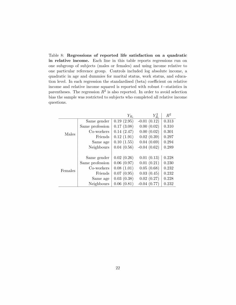
Table 8: Regressions of reported life satisfaction on a quadraticin relative income. Each line in this table reports regressions run onone subgroup of subjects (males or females) and using income relative toone particular reference group. Controls included log absolute income, aquadratic in age and dummies for marital status, work status, and educa-tion level. In each regression the standardised (beta) coefficient on relativeincome and relative income squared is reported with robust t−statistics inparentheses. The regression R2 is also reported. In order to avoid selectionbias the sample was restricted to subjects who completed all relative incomequestions.

YRi Y 2Ri

R2

Males

Same gender 0.19 (2.95) -0.01 (0.12) 0.313Same profession 0.17 (3.08) 0.00 (0.02) 0.310

Co-workers 0.14 (2.47) 0.00 (0.02) 0.301Friends 0.12 (1.91) 0.02 (0.39) 0.297

Same age 0.10 (1.55) 0.04 (0.69) 0.294Neighbours 0.04 (0.56) -0.04 (0.62) 0.289

Females

Same gender 0.02 (0.26) 0.01 (0.13) 0.228Same profession 0.06 (0.97) 0.01 (0.21) 0.230

Co-workers 0.08 (1.01) 0.05 (0.68) 0.232Friends 0.07 (0.95) 0.03 (0.45) 0.232

Same age 0.03 (0.38) 0.02 (0.27) 0.228Neighbours 0.06 (0.81) -0.04 (0.77) 0.232

22