Available online at www.sciencedirect.com

www.elsevier.com/locate/wasman

Waste Management 28 (2008) 2552–2564

Life cycle assessment of urban waste management: Energyperformances and environmental impacts. The case of Rome, Italy

Francesco Cherubini a,*, Silvia Bargigli b, Sergio Ulgiati b

a Joanneum Research, Elisabethstraße 5, 8010, Graz, Austriab Universita degli Studi di Napoli ‘‘Parthenope”, Dipartimento di Scienze per l’Ambiente, Centro Direzionale, Isola C4, 80133 Napoli, Italy

Accepted 21 November 2007Available online 29 January 2008

Abstract

Landfilling is nowadays the most common practice of waste management in Italy in spite of enforced regulations aimed at increasingwaste pre-sorting as well as energy and material recovery. In this work we analyse selected alternative scenarios aimed at minimizing theunused material fraction to be delivered to the landfill. The methodological framework of the analysis is the life cycle assessment, in amulti-method form developed by our research team. The approach was applied to the case of municipal solid waste (MSW) managementin Rome, with a special focus on energy and material balance, including global and local scale airborne emissions. Results, provided inthe form of indices and indicators of efficiency, effectiveness and environmental impacts, point out landfill activities as the worst wastemanagement strategy at a global scale. On the other hand, the investigated waste treatments with energy and material recovery allowimportant benefits of greenhouse gas emission reduction (among others) but are still affected by non-negligible local emissions. Further-more, waste treatments leading to energy recovery provide an energy output that, in the best case, is able to meet 15% of the Rome elec-tricity consumption.� 2007 Elsevier Ltd. All rights reserved.

1. Introduction

Humanity lives in a closed system, the Earth, where theamount of matter is almost constant and is continuouslyrecycled among Biosphere, Lithosphere, Atmosphere andHydrosphere by sun-powered and geothermal processes.The Earth is able to exchange a large amount of energywith the surrounding space, but only a little amount ofmatter. The continuous cycling of matter is therefore fun-damental for the survival of the biosphere and humankind.

The problem is that many chemicals and materialsderived from human activities are not recyclable by naturalprocesses in relatively short times and require additionaltechnological processing. Such transformation processes(landfill, incineration, gasification, or recycling, amongothers) require energy.

0956-053X/$ - see front matter � 2007 Elsevier Ltd. All rights reserved.

doi:10.1016/j.wasman.2007.11.011

* Corresponding author. Tel.: +43 3168761327; fax: +43 3168761330.E-mail address: cherufra@yahoo.it (F. Cherubini).

The present study focuses on the environmental assess-ment of selected solid waste management options that wereproposed for the municipality of Rome, Italy. The city hasan area of 1.29E+09 m2, 2.81E+06 inhabitants and a pro-duction of Municipal Solid Wastes (MSW) equal to1.46E+12 g per yr. Pre-sorted wastes are not included inour figures, due to their relatively small amount, althoughthe municipal waste management company, AMA, is dis-playing increasing efforts towards pre-sorting and recyclingof still usable materials. The evaluation of MSW manage-ment of Rome is part of a larger project aimed at the studyof material and energy performances and dynamics ofselected Italian and international cities. Rome, the capitalof Italy, is also the larger Italian urban system and waschosen as the starting point and reference case for furtherinvestigation of other Italian cities.

Most MSW in Rome is currently disposed of in thelandfill of Malagrotta (Rome), with no further sortingand/or thermal conversion. This short-sighted practice islikely to lead to exhaustion of the landfill area in a couple

F. Cherubini et al. / Waste Management 28 (2008) 2552–2564 2553

of years and therefore is not sustainable. The aim of thispaper is to compare selected waste disposal alternatives,highlighting those able to minimize the amount of wasteand maximize material and energy recovery.

1.1. Scope of the assessment: the scenarios

The applied life cycle assessment procedure (ISO 14040,1997) is an internationally standardized method that is con-sidered one of the most effective management tools foridentifying and assessing the environmental impacts relatedto industrial processes and waste management options(Clift et al., 2000). In the present paper, the waste collectionstep is firstly investigated and, afterwards, the followingfour different scenarios are analyzed:

� Scenario 0: Wastes are delivered to landfill without anyfurther treatment (the present case of Rome).� Scenario 1: Part of the biogas naturally released by the

landfill is collected, treated and burnt to produceelectricity.� Scenario 2: A sorting plant at landfill site separates the

organic and inorganic fractions. Ferrous componentsare also recovered and sent to recycling. Electricity, bio-gas (from anaerobic digestion) and compost are thenproduced.� Scenario 3: Wastes are directly incinerated to produce

electricity with no further pre-sorting or pre-treating.

1.2. Zero emission/zero waste strategies

Waste management strategies should aim at maximizingenergy and material recovery while minimizing the finalamount of waste delivered to landfill and the pollutionrelated to all treatment and collection steps. These targetsare only reachable by implementing waste minimizationpolicies and waste pre-sorting practices, in conjunctionwith appropriate technological options within a zero emis-sion/zero waste framework that emulates natural cyclesand dynamics. Ecosystems recycle every kind of waste,and the concept itself of ‘‘waste” is no longer appropriate.The products from one component or compartment arealways a useful resource for another component or com-partment. Ecosystems self-organize in such a way that allavailable resources are utilized to the maximum possibleextent and no unused resources are left.1

1 This may not be true for each individual process over a short timescale, but depends on the spatial and time window of interest as well as onthe number of interacting processes. For example, fossil fuels (reducedcarbon) can be considered as the waste of photosynthesis, a process whereproduction is slightly larger than consumption (respiration). Instead, onthe larger geological scales these materials are also cycled by earth’sconvective processes and are used for the global construction of earthcrust. By extracting them, humans boost the process by returning carbonto the biosphere faster than it would have been via natural cycles.

The detritus chain in ecosystems is a clear example ofthis statement. Human dominated systems should bereshaped according to the same principle, for maximumresource use and zero emissions (Pauli, 1998; Schnitzerand Ulgiati, 2007). Instead, in traditional linear productionand consumption systems, resources are processed andpassed on to the next step, and unused wastes are releasedto the environment. As a consequence, the energy andmaterial cost of the product is higher and the efficiency islower, and a higher emission load is imposed on the envi-ronment. Such systems are unlikely to develop maximum-power behaviour and therefore be successful in mediumand long-term competition, when resources becomescarcer.

In an integrated zero emission/zero waste strategy,waste prevention should become a priority. Processes arereorganized and clustered in such a way that unusedresources become the raw input to new production pat-terns. When resources become scarce, this behaviour trans-lates into a selective advantage. While in conventionalproduction the main resources are matter, energy andlabour, zero-emission patterns rely to a larger extent onknowledge, i.e., on better information about the needs ofand surpluses from each component as well as about tech-nological tools for resource processing and exchange (Gra-vitis and Suzuki, 1999).

2. Method of analysis (Life cycle assessment – LCA) and

system description

The methodological framework used in this paper is anextended life cycle assessment, where several evaluationmethods are jointly used in order to provide a set of com-plementary indicators at multiple scales, based on the sameset of input data (Ulgiati et al., 2006).

2.1. The methodology for the assessment

Generally speaking, all impact assessment methods canbe divided into two broad categories: those that focus onthe amount of resources used per unit of product(‘‘upstream” methods), and those that deal with the fateof a system’s emissions (‘‘downstream” methods). The for-mer can provide invaluable insights into the hidden envi-ronmental costs and inherent (un)sustainability of evenseemingly ‘‘clean” systems. On the other hand, downstreammethods are often more closely related to the immediateperceived impact on the local ecosystem, and can unveillarge differences between systems with similar upstreamperformance.

It must be realised that in no circumstance can a singlemethod be sufficient to provide comprehensive informationon an environmental impact assessment, and that LCAsbased on only one approach invariably end up providingpartial and sometimes even counterproductive indications.A complete LCA should carefully rely on a selection ofimpact assessment methods, which account for both the

2554 F. Cherubini et al. / Waste Management 28 (2008) 2552–2564

upstream and the downstream categories. Early efforts ofthe scientific community in this direction can be recognisedin the scientific literature (Ulgiati, 2000; Khan et al., 2002,among others).

The Material Flow Accounting method (Schmidt-Bleek,1993; Hinterberger and Stiller, 1998; Bargigli et al., 2005)aims at evaluating the environmental disturbance associ-ated with the withdrawal or diversion of material flowsfrom their natural ecosystemic pathways. In this method,appropriate material intensity factors (g/unit) are multi-plied by each input, respectively, accounting for the totalamount of abiotic matter, water, air and biotic matterdirectly or indirectly required to provide that very sameinput to the system. The resulting material intensities(MIs) of the individual inputs are then summed togetherfor each environmental compartment (again: abiotic mat-ter, water, air and biotic matter), and assigned to the sys-tem’s output as a quantitative measure of its cumulativeenvironmental burden from that compartment (oftenreferred to as ‘‘Ecological Rucksack”).

The Embodied Energy Analysis method (Herendeen,1998; IFIAS, 1974) deals with the gross (direct and indi-rect) energy requirement of the analysed system, and offersuseful insight on the first-law energy efficiency of the ana-lysed system on the global scale, taking into considerationall of the employed commercial energy supplies. In thismethod, all of the material and energy inputs to the ana-lysed system are multiplied by appropriate oil equivalentfactors (g/unit), and the cumulative embodied energyrequirement of the system’s output is then computed asthe sum of the individual oil equivalents of the inputs,which can be converted to energy units by multiplying bythe standard crude oil equivalency factor of 41.860 J/g.The chosen cumulative indicator is the so-called ‘‘GrossEnergy Requirement” (GER), expressing the total com-mercial energy requirement of one unit of output in termsof equivalent Joules of petroleum oil.

The Emergy Accounting method (Brown and Ulgiati,2004; Odum, 1988, 1996) also looks at the environmentalperformance of the system on a global scale, but this timealso taking into account all of the free environmentalinputs such as sunlight, wind, and rain, as well as the indi-rect environmental support embodied in human labor andservices, which are not usually included in traditionalembodied energy analyses. Moreover, the accounting isextended back in time to include the environmental workneeded for resource formation (and consequent renewabil-ity). All inputs are accounted for in terms of their solaremergy, defined as the total amount of solar availableenergy (exergy) directly or indirectly required to make agiven product or support a given flow, and measured insolar equivalent Joules (seJ). The amount of emergy thatwas originally required to provide one unit of each inputis referred to as its specific emergy (seJ/unit) or transformi-ty (seJ/J), and can be considered a ‘‘quality” factor whichfunctions as a measure of the intensity of the support pro-vided by the biosphere to the input under study. Likewise,

the specific emergy or transformity of the system’s output iscalculated as the sum of the total emergy embodied in thenecessary inputs to the system divided by the output massor exergy. The total emergy requirement thus calculatedcan be interpreted as an indication of the total environmen-tal service appropriation by the analysed human activity.In particular, while the total non-renewable emergy inputto the system under study provides a quantitative estimateof global non-renewable resource depletion, the totalrenewable emergy requirement is a measure of all of thenatural exchange-pool resources diverted from their natu-ral pathways, and that can therefore no longer providetheir natural ecosystemic functions. The ecological rele-vance of the emergy methodology was recently discussedin detail by Brown and Hall, 2004), where the scientificcareer of its founder, Odum, is illustrated.

2.2. System description

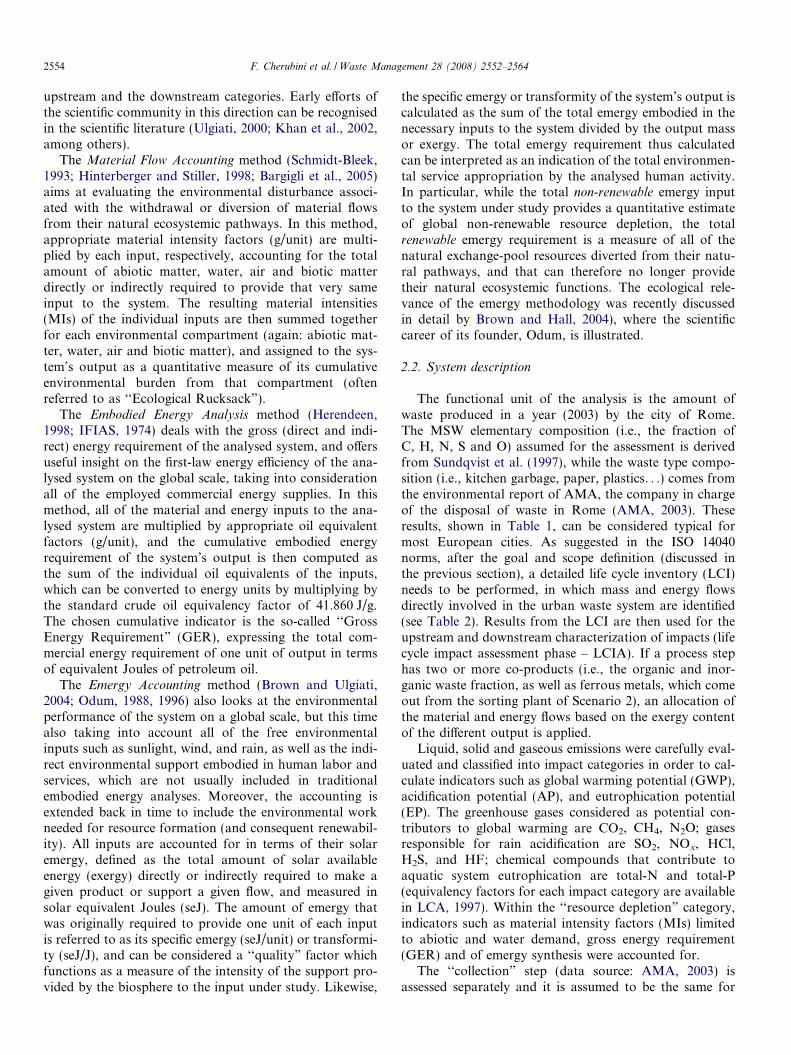
The functional unit of the analysis is the amount ofwaste produced in a year (2003) by the city of Rome.The MSW elementary composition (i.e., the fraction ofC, H, N, S and O) assumed for the assessment is derivedfrom Sundqvist et al. (1997), while the waste type compo-sition (i.e., kitchen garbage, paper, plastics. . .) comes fromthe environmental report of AMA, the company in chargeof the disposal of waste in Rome (AMA, 2003). Theseresults, shown in Table 1, can be considered typical formost European cities. As suggested in the ISO 14040norms, after the goal and scope definition (discussed inthe previous section), a detailed life cycle inventory (LCI)needs to be performed, in which mass and energy flowsdirectly involved in the urban waste system are identified(see Table 2). Results from the LCI are then used for theupstream and downstream characterization of impacts (lifecycle impact assessment phase – LCIA). If a process stephas two or more co-products (i.e., the organic and inor-ganic waste fraction, as well as ferrous metals, which comeout from the sorting plant of Scenario 2), an allocation ofthe material and energy flows based on the exergy contentof the different output is applied.

Liquid, solid and gaseous emissions were carefully eval-uated and classified into impact categories in order to cal-culate indicators such as global warming potential (GWP),acidification potential (AP), and eutrophication potential(EP). The greenhouse gases considered as potential con-tributors to global warming are CO2, CH4, N2O; gasesresponsible for rain acidification are SO2, NOx, HCl,H2S, and HF; chemical compounds that contribute toaquatic system eutrophication are total-N and total-P(equivalency factors for each impact category are availablein LCA, 1997). Within the ‘‘resource depletion” category,indicators such as material intensity factors (MIs) limitedto abiotic and water demand, gross energy requirement(GER) and of emergy synthesis were accounted for.

The ‘‘collection” step (data source: AMA, 2003) isassessed separately and it is assumed to be the same for

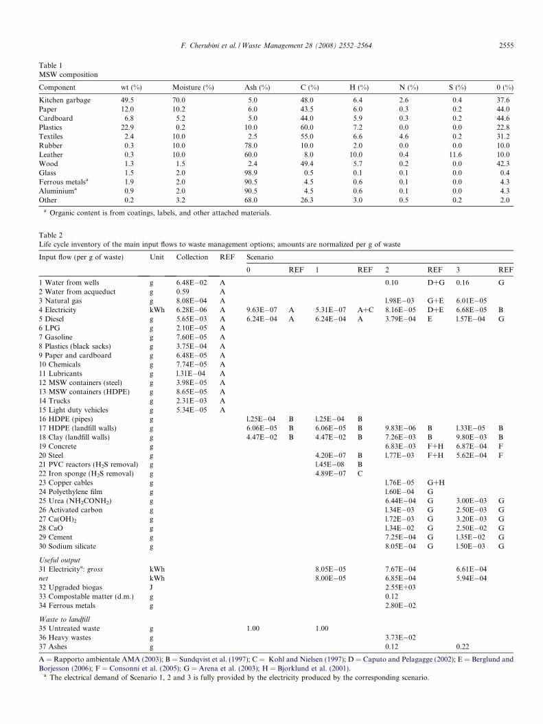
Table 1MSW composition

Component wt (%) Moisture (%) Ash (%) C (%) H (%) N (%) S (%) 0 (%)

Kitchen garbage 49.5 70.0 5.0 48.0 6.4 2.6 0.4 37.6Paper 12.0 10.2 6.0 43.5 6.0 0.3 0.2 44.0Cardboard 6.8 5.2 5.0 44.0 5.9 0.3 0.2 44.6Plastics 22.9 0.2 10.0 60.0 7.2 0.0 0.0 22.8Textiles 2.4 10.0 2.5 55.0 6.6 4.6 0.2 31.2Rubber 0.3 10.0 78.0 10.0 2.0 0.0 0.0 10.0Leather 0.3 10.0 60.0 8.0 10.0 0.4 11.6 10.0Wood 1.3 1.5 2.4 49.4 5.7 0.2 0.0 42.3Glass 1.5 2.0 98.9 0.5 0.1 0.1 0.0 0.4Ferrous metalsa 1.9 2.0 90.5 4.5 0.6 0.1 0.0 4.3Aluminiuma 0.9 2.0 90.5 4.5 0.6 0.1 0.0 4.3Other 0.2 3.2 68.0 26.3 3.0 0.5 0.2 2.0

a Organic content is from coatings, labels, and other attached materials.

Table 2Life cycle inventory of the main input flows to waste management options; amounts are normalized per g of waste

Input flow (per g of waste) Unit Collection REF Scenario

0 REF 1 REF 2 REF 3 REF

1 Water from wells g 6.48E�02 A 0.10 D+G 0.16 G2 Water from acqueduct g 0.59 A3 Natural gas g 8.08E�04 A l.98E�03 G+E 6.01E�054 Electricity kWh 6.28E�06 A 9.63E�07 A 5.31E�07 A+C 8.16E�05 D+E 6.68E�05 B5 Diesel g 5.65E�03 A 6.24E�04 A 6.24E�04 A 3.79E�04 E l.57E�04 G6 LPG g 2.10E�05 A7 Gasoline g 7.60E�05 A8 Plastics (black sacks) g 3.75E�04 A9 Paper and cardboard g 6.48E�05 A10 Chemicals g 7.74E�05 A11 Lubricants g l.31E�04 A12 MSW containers (steel) g 3.98E�05 A13 MSW containers (HDPE) g 8.65E�05 A14 Trucks g 2.31E�03 A15 Light duty vehicles g 5.34E�05 A16 HDPE (pipes) g l.25E�04 B l.25E�04 B17 HDPE (landfill walls) g 6.06E�05 B 6.06E�05 B 9.83E�06 B l.33E�05 B18 Clay (landfill walls) g 4.47E�02 B 4.47E�02 B 7.26E�03 B 9.80E�03 B19 Concrete g 6.83E�03 F+H 6.87E�04 F20 Steel g 4.20E�07 B l.77E�03 F+H 5.62E�04 F21 PVC reactors (H2S removal) g l.45E�08 B22 Iron sponge (H2S removal) g 4.89E�07 C23 Copper cables g l.76E�05 G+H24 Polyethylene film g l.60E�04 G25 Urea (NH2CONH2) g 6.44E�04 G 3.00E�03 G26 Activated carbon g l.34E�03 G 2.50E�03 G27 Ca(OH)2 g l.72E�03 G 3.20E�03 G28 CaO g l.34E�02 G 2.50E�02 G29 Cement g 7.25E�04 G l.35E�02 G30 Sodium silicate g 8.05E�04 G l.50E�03 G

Useful output

31 Electricitya: gross kWh 8.05E�05 7.67E�04 6.61E�04net kWh 8.00E�05 6.85E�04 5.94E�0432 Upgraded biogas J 2.55E+0333 Compostable matter (d.m.) g 0.1234 Ferrous metals g 2.80E�02

Waste to landfill

35 Untreated waste g 1.00 1.0036 Heavy wastes g 3.73E�0237 Ashes g 0.12 0.22

A = Rapporto ambientale AMA (2003); B = Sundqvist et al. (1997); C = Kohl and Nielsen (1997); D = Caputo and Pelagagge (2002); E = Berglund andBorjesson (2006); F = Consonni et al. (2005); G = Arena et al. (2003); H = Bjorklund et al. (2001).

a The electrical demand of Scenario 1, 2 and 3 is fully provided by the electricity produced by the corresponding scenario.

F. Cherubini et al. / Waste Management 28 (2008) 2552–2564 2555

2556 F. Cherubini et al. / Waste Management 28 (2008) 2552–2564

the four scenarios. Waste collection in Rome is based onheavy duty diesel-fuelled trucks which pick up the un-pre-sorted wastes from large MSW containers located atthe sidewalk and/or roadside of the whole city area. Thereason why the collection is separately analysed is that itcan be significantly different from city to city and thereforemight hide the real results of the analysis of waste manage-ment strategies. By splitting the collection and the treat-ment steps, results are more likely to be comparable withand applicable to other urban systems.

Usually, the output of a scenario is composed of twotypes of energy (electricity and/or biogas); we consider thatpart of this amount is used as a feedback for internalenergy consumption within the landfilling/waste treatmentfacility. Regarding global impact indicators (i.e., GWP andAP), when one of the scenarios has an energy output thenet results are shown.

Environmental benefits derived from the recycled mate-rial (ferrous metals and compostable matter) are notaccounted for, due to the uncertainty of available data.

Scenario 0: the landfill. Wastes are collected and buriedin a monitored landfill. For more information about alandfill system, see Sundqvist et al., 1997. In this systemthe organic fraction of waste undergoes decomposition inanaerobic conditions, releasing the so-called ‘‘landfill gas”.This is mainly composed of CH4 (58%) and CO2 (41%), butit may also contain traces of H2S, HCl, HF and otherchemical compounds. On a yearly basis, a methane produc-tion of 140 m3 per ton of landfilled waste is estimated(Sundqvist et al., 1997), generating a CH4 emission of2.04E+08 m3 at atmospheric pressure and density (2003data). Fifty percent of the biogas is assumed to be collectedby pipes and burnt in flares to convert CH4 intoCO2(mainly). Such a CO2 emission from landfill gas flaringis quantified but it is not accounted for in the GWP becauseit does not have a fossil origin (it comes from the organicfraction, because plastic does not decompose); the remain-ing 50% of landfill biogas is assumed to be directly releasedto the atmosphere.

Other basic assumptions regarding landfill activities(Scenarios 0 and 1) are:

� Three percent of the total sulphur disposed of to landfillin 1 yr is released to atmosphere as H2S (Nielsen andHauschild, 1998);� The main emissions released from biogas combustion in

flares are CO, NO2, HCl, HF (emission factors: 800,100, 12 and 0.02 mg/m3, respectively (White et al.,1999)) and dioxins (emission factors from USEPA,1995);� The main emissions freely released from the landfill

together with biogas (CH4 and CO2) are CO, HCl andHF (emission factors: 13, 65 and 13 mg/m3, respectively(White et al., 1999));� Heavy metals released to atmosphere are only mercury

(Hg) and cadmium (Cd), the most volatiles (Sundqvistet al., 1997);

� Leachate emission (and its composition) is averagedfrom several data reported by Kylefors, 2003.

According to such assumptions, the airborne emissionsdue to combustion processes directly or indirectly involvedin the system are evaluated (as well as for Scenarios 1–3):

� Emissions from spontaneous landfill fires (CO2, CO,NOx, and dioxins among others (Sundqvist et al.,1997)); regarding dioxins, HPA and PCB emissions,since they are mostly absorbed to the particle matters,they fall down to the ground close to the point fromwhere they are emitted, and then only 35% of thisamount is treated as emission.� Emissions released from the combustion of fossil fuels

(natural gas, diesel, gasoline, liquid propane gas): CO2,CO, NOx, PM10, SO2, CH4, N2O (EPA, 1996) and diox-ins (USEPA, 1995). Emission factors for transportationfuels can be found in APAT (1999).� Emissions for electricity production required to feed the

system; the Italian electric supply mix was considered(coal 14.2%, oil 30.8%, natural gas 34.8%, hydro16.6%, other renewable 3.6%).� Emissions for production and delivering of the input

flows required by the system.� All dioxin and furan emissions are referred to g of

2,3,7,8-TCDD with apposite equivalent factors (USEP-A, 1995).

In this scenario, the most relevant input flows are clayand earth for landfill walls (Table 2).

Scenario 1: landfill with biogas recovery. The biogas nat-urally released from the landfill is collected (about 50% ofthe total), treated (in PVC reactors in order to remove H2Swith iron sponge) and burnt (in situ) in order to produceelectricity. The remaining biogas fraction is burnt in flares(25%) or released to the atmosphere (25%). As mentionedfor the previous scenario, also in this case the CO2 releasedby biogas combustion was not accounted for as contribut-ing to the GWP (however, it was included among the localemissions). The total energy content of the collected biogasis estimated to be 3.12E+09 MJ, thanks to its lower heatingvalue (LHV) equal to 17.73 MJ/m3 (Conte, 2001). The bio-gas is burnt in turbines with a 28% efficiency to produce2.43E+08 kWh of electricity per year. Emission factorsfor the combustion of biogas are: NOx 349.56 mg/m3;CO 120.95 mg/m3; PM10 2.68 mg/m3; SO2 6.83 mg/m3;H2S 0.51 mg/m3; HCl 3.97 mg/m3; and HF 1.00 mg/m3(Conte, 2001). Material inputs for biogas collectionand use can be considered negligible in terms of mass con-tribution compared to the clay and earth for the landfillwalls (as indicated in Table 2).

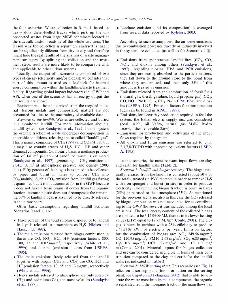
Scenario 2: MSW sorting plant. This scenario (see Fig. 1)relies on a sorting plant (for information on the sortingplant, see Caputo and Pelagagge, 2002) that is able to sep-arate the waste mass into its main components; the organicis separated from the inorganic fraction (the main flows), as

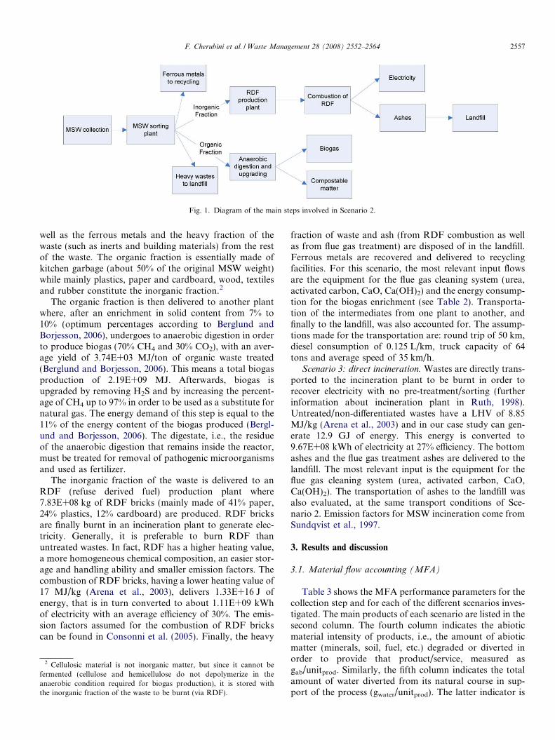
Fig. 1. Diagram of the main steps involved in Scenario 2.

F. Cherubini et al. / Waste Management 28 (2008) 2552–2564 2557

well as the ferrous metals and the heavy fraction of thewaste (such as inerts and building materials) from the restof the waste. The organic fraction is essentially made ofkitchen garbage (about 50% of the original MSW weight)while mainly plastics, paper and cardboard, wood, textilesand rubber constitute the inorganic fraction.2

The organic fraction is then delivered to another plantwhere, after an enrichment in solid content from 7% to10% (optimum percentages according to Berglund andBorjesson, 2006), undergoes to anaerobic digestion in orderto produce biogas (70% CH4 and 30% CO2), with an aver-age yield of 3.74E+03 MJ/ton of organic waste treated(Berglund and Borjesson, 2006). This means a total biogasproduction of 2.19E+09 MJ. Afterwards, biogas isupgraded by removing H2S and by increasing the percent-age of CH4 up to 97% in order to be used as a substitute fornatural gas. The energy demand of this step is equal to the11% of the energy content of the biogas produced (Bergl-und and Borjesson, 2006). The digestate, i.e., the residueof the anaerobic digestion that remains inside the reactor,must be treated for removal of pathogenic microorganismsand used as fertilizer.

The inorganic fraction of the waste is delivered to anRDF (refuse derived fuel) production plant where7.83E+08 kg of RDF bricks (mainly made of 41% paper,24% plastics, 12% cardboard) are produced. RDF bricksare finally burnt in an incineration plant to generate elec-tricity. Generally, it is preferable to burn RDF thanuntreated wastes. In fact, RDF has a higher heating value,a more homogeneous chemical composition, an easier stor-age and handling ability and smaller emission factors. Thecombustion of RDF bricks, having a lower heating value of17 MJ/kg (Arena et al., 2003), delivers 1.33E+16 J ofenergy, that is in turn converted to about 1.11E+09 kWhof electricity with an average efficiency of 30%. The emis-sion factors assumed for the combustion of RDF brickscan be found in Consonni et al. (2005). Finally, the heavy

2 Cellulosic material is not inorganic matter, but since it cannot befermented (cellulose and hemicellulose do not depolymerize in theanaerobic condition required for biogas production), it is stored withthe inorganic fraction of the waste to be burnt (via RDF).

fraction of waste and ash (from RDF combustion as wellas from flue gas treatment) are disposed of in the landfill.Ferrous metals are recovered and delivered to recyclingfacilities. For this scenario, the most relevant input flowsare the equipment for the flue gas cleaning system (urea,activated carbon, CaO, Ca(OH)2) and the energy consump-tion for the biogas enrichment (see Table 2). Transporta-tion of the intermediates from one plant to another, andfinally to the landfill, was also accounted for. The assump-tions made for the transportation are: round trip of 50 km,diesel consumption of 0.125 L/km, truck capacity of 64tons and average speed of 35 km/h.

Scenario 3: direct incineration. Wastes are directly trans-ported to the incineration plant to be burnt in order torecover electricity with no pre-treatment/sorting (furtherinformation about incineration plant in Ruth, 1998).Untreated/non-differentiated wastes have a LHV of 8.85MJ/kg (Arena et al., 2003) and in our case study can gen-erate 12.9 GJ of energy. This energy is converted to9.67E+08 kWh of electricity at 27% efficiency. The bottomashes and the flue gas treatment ashes are delivered to thelandfill. The most relevant input is the equipment for theflue gas cleaning system (urea, activated carbon, CaO,Ca(OH)2). The transportation of ashes to the landfill wasalso evaluated, at the same transport conditions of Sce-nario 2. Emission factors for MSW incineration come fromSundqvist et al., 1997.

3. Results and discussion

3.1. Material flow accounting (MFA)

Table 3 shows the MFA performance parameters for thecollection step and for each of the different scenarios inves-tigated. The main products of each scenario are listed in thesecond column. The fourth column indicates the abioticmaterial intensity of products, i.e., the amount of abioticmatter (minerals, soil, fuel, etc.) degraded or diverted inorder to provide that product/service, measured asgab/unitprod. Similarly, the fifth column indicates the totalamount of water diverted from its natural course in sup-port of the process (gwater/unitprod). The latter indicator is

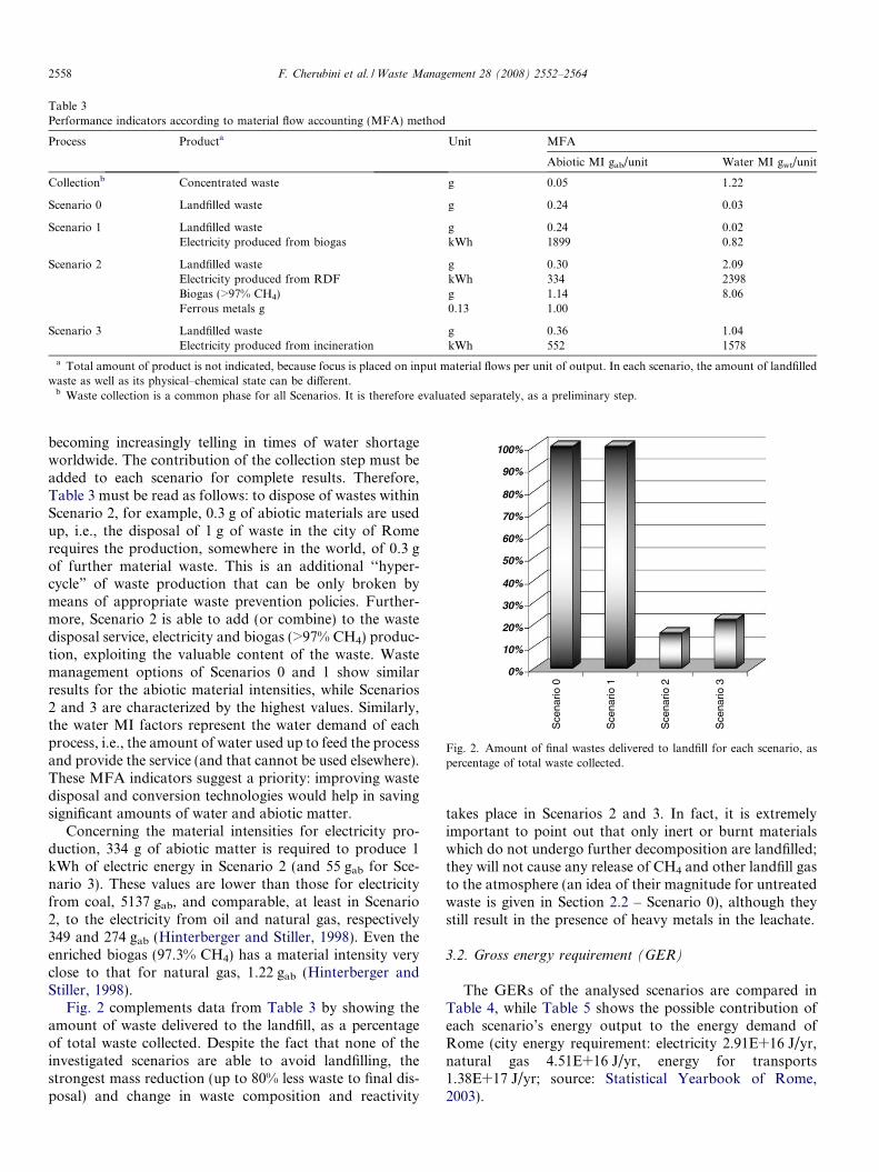
Table 3Performance indicators according to material flow accounting (MFA) method

Process Producta Unit MFA

Abiotic MI gab/unit Water MI gwt/unit

Collectionb Concentrated waste g 0.05 1.22

Scenario 0 Landfilled waste g 0.24 0.03

Scenario 1 Landfilled waste g 0.24 0.02Electricity produced from biogas kWh 1899 0.82

Scenario 2 Landfilled waste g 0.30 2.09Electricity produced from RDF kWh 334 2398Biogas (>97% CH4) g 1.14 8.06Ferrous metals g 0.13 1.00

Scenario 3 Landfilled waste g 0.36 1.04Electricity produced from incineration kWh 552 1578

a Total amount of product is not indicated, because focus is placed on input material flows per unit of output. In each scenario, the amount of landfilledwaste as well as its physical–chemical state can be different.

b Waste collection is a common phase for all Scenarios. It is therefore evaluated separately, as a preliminary step.

0%

10%

20%

30%

40%

50%

60%

70%

80%

90%

100%

Sce

nario

0

Sce

nario

1

Sce

nario

2

Sce

nario

3

Fig. 2. Amount of final wastes delivered to landfill for each scenario, aspercentage of total waste collected.

2558 F. Cherubini et al. / Waste Management 28 (2008) 2552–2564

becoming increasingly telling in times of water shortageworldwide. The contribution of the collection step must beadded to each scenario for complete results. Therefore,Table 3 must be read as follows: to dispose of wastes withinScenario 2, for example, 0.3 g of abiotic materials are usedup, i.e., the disposal of 1 g of waste in the city of Romerequires the production, somewhere in the world, of 0.3 gof further material waste. This is an additional ‘‘hyper-cycle” of waste production that can be only broken bymeans of appropriate waste prevention policies. Further-more, Scenario 2 is able to add (or combine) to the wastedisposal service, electricity and biogas (>97% CH4) produc-tion, exploiting the valuable content of the waste. Wastemanagement options of Scenarios 0 and 1 show similarresults for the abiotic material intensities, while Scenarios2 and 3 are characterized by the highest values. Similarly,the water MI factors represent the water demand of eachprocess, i.e., the amount of water used up to feed the processand provide the service (and that cannot be used elsewhere).These MFA indicators suggest a priority: improving wastedisposal and conversion technologies would help in savingsignificant amounts of water and abiotic matter.

Concerning the material intensities for electricity pro-duction, 334 g of abiotic matter is required to produce 1kWh of electric energy in Scenario 2 (and 55 gab for Sce-nario 3). These values are lower than those for electricityfrom coal, 5137 gab, and comparable, at least in Scenario2, to the electricity from oil and natural gas, respectively349 and 274 gab (Hinterberger and Stiller, 1998). Even theenriched biogas (97.3% CH4) has a material intensity veryclose to that for natural gas, 1.22 gab (Hinterberger andStiller, 1998).

Fig. 2 complements data from Table 3 by showing theamount of waste delivered to the landfill, as a percentageof total waste collected. Despite the fact that none of theinvestigated scenarios are able to avoid landfilling, thestrongest mass reduction (up to 80% less waste to final dis-posal) and change in waste composition and reactivity

takes place in Scenarios 2 and 3. In fact, it is extremelyimportant to point out that only inert or burnt materialswhich do not undergo further decomposition are landfilled;they will not cause any release of CH4 and other landfill gasto the atmosphere (an idea of their magnitude for untreatedwaste is given in Section 2.2 – Scenario 0), although theystill result in the presence of heavy metals in the leachate.

3.2. Gross energy requirement (GER)

The GERs of the analysed scenarios are compared inTable 4, while Table 5 shows the possible contribution ofeach scenario’s energy output to the energy demand ofRome (city energy requirement: electricity 2.91E+16 J/yr,natural gas 4.51E+16 J/yr, energy for transports1.38E+17 J/yr; source: Statistical Yearbook of Rome,2003).

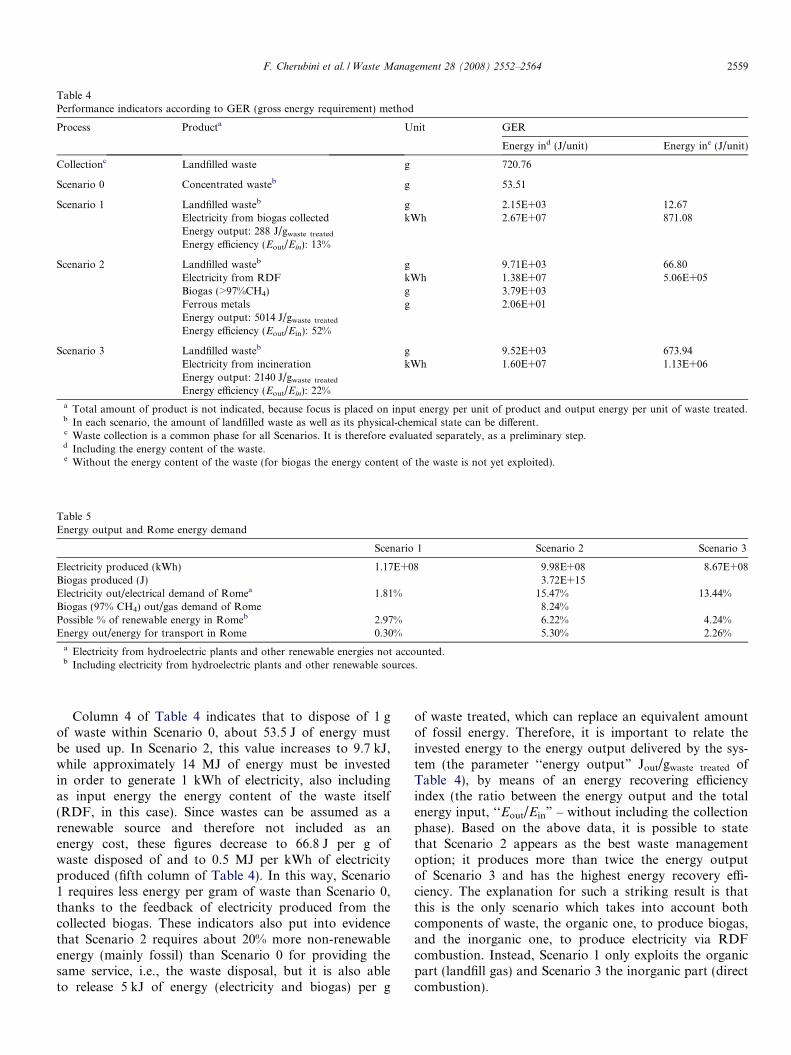
Table 4Performance indicators according to GER (gross energy requirement) method

Process Producta Unit GER

Energy ind (J/unit) Energy ine (J/unit)

Collectionc Landfilled waste g 720.76

Scenario 0 Concentrated wasteb g 53.51

Scenario 1 Landfilled wasteb g 2.15E+03 12.67Electricity from biogas collected kWh 2.67E+07 871.08Energy output: 288 J/gwaste treated

Energy efficiency (Eout/Ein): 13%

Scenario 2 Landfilled wasteb g 9.71E+03 66.80Electricity from RDF kWh 1.38E+07 5.06E+05Biogas (>97%CH4) g 3.79E+03Ferrous metals g 2.06E+01Energy output: 5014 J/gwaste treated

Energy efficiency (Eout/Ein): 52%

Scenario 3 Landfilled wasteb g 9.52E+03 673.94Electricity from incineration kWh 1.60E+07 1.13E+06Energy output: 2140 J/gwaste treated

Energy efficiency (Eout/Ein): 22%

a Total amount of product is not indicated, because focus is placed on input energy per unit of product and output energy per unit of waste treated.b In each scenario, the amount of landfilled waste as well as its physical-chemical state can be different.c Waste collection is a common phase for all Scenarios. It is therefore evaluated separately, as a preliminary step.d Including the energy content of the waste.e Without the energy content of the waste (for biogas the energy content of the waste is not yet exploited).

Table 5Energy output and Rome energy demand

Scenario 1 Scenario 2 Scenario 3

Electricity produced (kWh) 1.17E+08 9.98E+08 8.67E+08Biogas produced (J) 3.72E+15Electricity out/electrical demand of Romea 1.81% 15.47% 13.44%Biogas (97% CH4) out/gas demand of Rome 8.24%Possible % of renewable energy in Romeb 2.97% 6.22% 4.24%Energy out/energy for transport in Rome 0.30% 5.30% 2.26%

a Electricity from hydroelectric plants and other renewable energies not accounted.b Including electricity from hydroelectric plants and other renewable sources.

F. Cherubini et al. / Waste Management 28 (2008) 2552–2564 2559

Column 4 of Table 4 indicates that to dispose of 1 gof waste within Scenario 0, about 53.5 J of energy mustbe used up. In Scenario 2, this value increases to 9.7 kJ,while approximately 14 MJ of energy must be investedin order to generate 1 kWh of electricity, also includingas input energy the energy content of the waste itself(RDF, in this case). Since wastes can be assumed as arenewable source and therefore not included as anenergy cost, these figures decrease to 66.8 J per g ofwaste disposed of and to 0.5 MJ per kWh of electricityproduced (fifth column of Table 4). In this way, Scenario1 requires less energy per gram of waste than Scenario 0,thanks to the feedback of electricity produced from thecollected biogas. These indicators also put into evidencethat Scenario 2 requires about 20% more non-renewableenergy (mainly fossil) than Scenario 0 for providing thesame service, i.e., the waste disposal, but it is also ableto release 5 kJ of energy (electricity and biogas) per g

of waste treated, which can replace an equivalent amountof fossil energy. Therefore, it is important to relate theinvested energy to the energy output delivered by the sys-tem (the parameter ‘‘energy output” Jout/gwaste treated ofTable 4), by means of an energy recovering efficiencyindex (the ratio between the energy output and the totalenergy input, ‘‘Eout/Ein” – without including the collectionphase). Based on the above data, it is possible to statethat Scenario 2 appears as the best waste managementoption; it produces more than twice the energy outputof Scenario 3 and has the highest energy recovery effi-ciency. The explanation for such a striking result is thatthis is the only scenario which takes into account bothcomponents of waste, the organic one, to produce biogas,and the inorganic one, to produce electricity via RDFcombustion. Instead, Scenario 1 only exploits the organicpart (landfill gas) and Scenario 3 the inorganic part (directcombustion).

Table 6Results of the emergy synthesis method

System Emergy demand with services (seJ/unit) Emergy demand without services (seJ/unit)

Collection step (gwaste) 1.27E+08 6.25E+07

Scenario 0 (gwaste) 1.58E+08 1.56E+08

Scenario 1:

Disposed waste (gwaste) 1.54E+08 1.52E+08Electricity (kWh) 5.36E+05 5.28E+05

Scenario 2:

Disposed waste (gwaste) 1.22E+08 1.16E+08Electricity (kWh) 2.28E+04 2.24E+04Upgraded biogas (g) 1.66E+04 1.60E+04Ferrous metals (g) 9.34E+07 6.48E+07

Scenario 3:Disposed waste (gwaste) 1.83E+08 1.81E+08Electricity (kWh) 8.56E+04 8.44E+04

3 That directly goes into the product/service or its manufacturing.4 That makes the input available to be exploited by the process.

2560 F. Cherubini et al. / Waste Management 28 (2008) 2552–2564

Table 4 also shows that in the present situation ofRome (collection + Scenario 0), the collection step ismore energy intensive than landfilling (due to the dieselconsumed by trucks); therefore, embodied energyanalysis points out a different priority than the one high-lighted by MFA: to minimize the fuel consumption ofthe collection step. Again, this is another proof of theneed for simultaneous and integrated application ofdifferent methods to the same process, not to hide someaspects of its dynamics.

Finally, a comparison among the energy demand forthe production of 1 kWh of electricity from differentsources can also be performed. The energy requirementsper kWh of electricity produced from Scenarios 1, 2 and3 are shown in the fourth and fifth columns of Table 4;these values are comparable with the energy demand forelectricity production by conventional sources, as oil(1.24E+07 J/kWh), coal (1.21E+07 J/kWh), natural gas(9.50E+06 J/kWh) and hydro (4.72E+06 J/kWh) (Fris-chknecht et al., 2003).

Table 5 shows that Scenario 2 could meet an importantfraction of Rome energy demand (15.47% of electricity and8.24% of natural gas) and would contribute to reach a tar-get of 6.22% of total city energy consumption (electricity,heating and transport) met by means of renewable sources(also including the contribution of hydroelectricity). If onlythe transport sector is taken into consideration, its renew-able energy fraction could be equal to 5.3%, very close tothe EU target of 5.75%, which must be achieved by the year2010. This seems to be the only way to meet such a targetwithout importing palm oil from Asia or bioethanol fromBrazil, given the low production of biofuels in Italy andtheir very difficult (if not impossible) implementation inthe short term.

3.3. Emergy synthesis

Table 6 shows results from emergy synthesis. The indica-tor chosen (among others available) is the ‘‘emergy inten-

sity”, i.e., the demand for direct3 and indirect4

environmental support per unit of waste treated or unit ofelectricity generated.

The emergy cost per gram of waste collected is muchlower than the cost per gram of waste processed, in eachof the four scenarios investigated. This is because of the rel-atively low emergy demand for machinery and fuel com-pared to the much larger demand for landfill construction(clay, concrete) in Scenarios 0 and 1, as well as for powermachinery in Scenarios 2 and 3. However, since emergyalso accounts for the environmental support to economicfactors, the collection step is the one with the largest emer-gy investment (labor of drivers and services for fuel).

Scenario 2 has the lower specific emergy per unit of dis-posed waste because it reduces the amount of waste sent tothe landfill, and as a consequence a much smaller landfill isrequired. However, the emergy cost for the several disposalsystems is on the same order of magnitude, and the differ-ent performance of the four scenarios is mainly based onthe quantity and quality of co-products they are able tosupply.

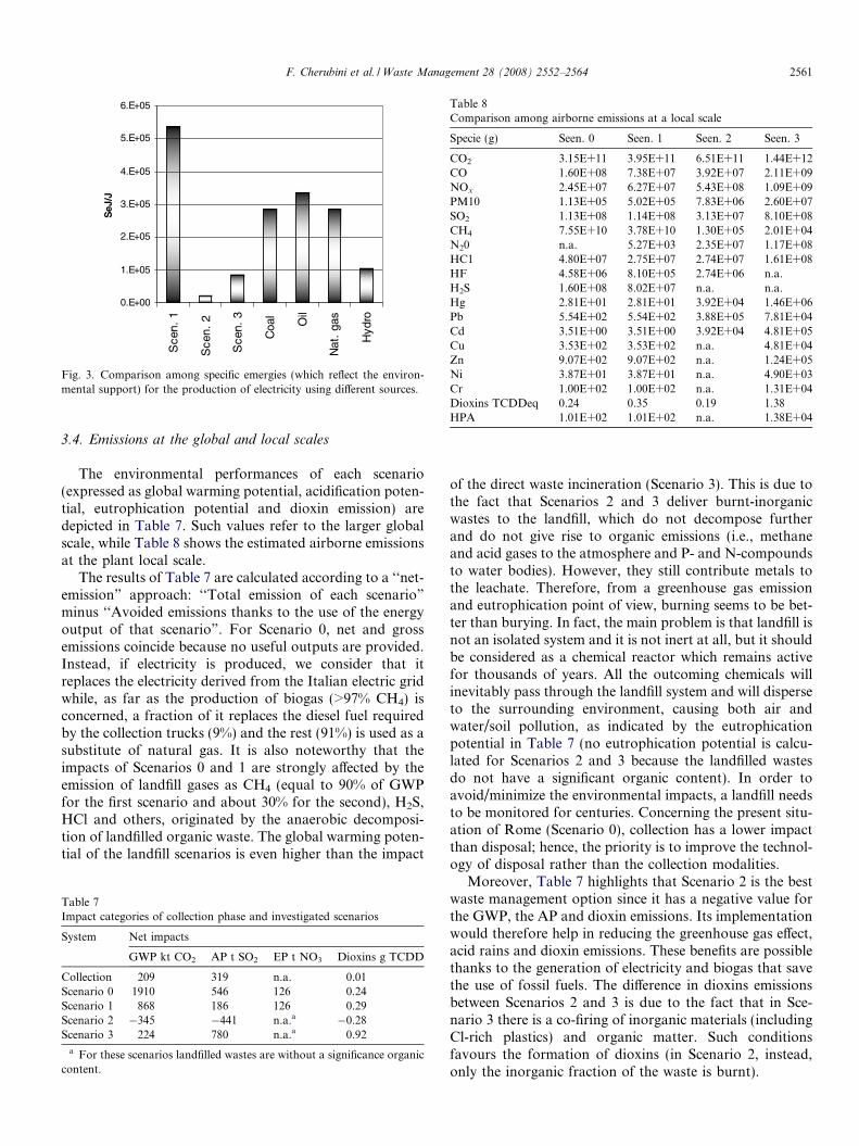
The specific emergy of electricity produced can be com-pared to that of common fossil fuel plants and hydro(Brown and Ulgiati, 2004), as shown in Fig. 3. Emergy syn-thesis clearly highlights the benefit of recycling. In fact, byassigning zero emergy (i.e., zero additional environmentalsupport) to the waste as such (Brown and Ulgiati, 2004),the emergy cost to be accounted for is only related to theadditional effort for collection and processing. Due to thefact that the emergy cost of recycled material is low com-pared to the emergy cost of new purchased input flows,the emergy intensities of the electricity produced in Scenar-ios 2 and 3 are the lowest, even compared with the emergyintensity of hydro-electricity. Therefore, recycling is arewarding practice requiring the least environmentalsupport.

0.E+00

1.E+05

2.E+05

3.E+05

4.E+05

5.E+05

6.E+05

Sce

n. 1

Sce

n. 2

Sce

n. 3

Coa

l

Oil

Nat

. ga

s

Hyd

ro

SeJ

/J

Fig. 3. Comparison among specific emergies (which reflect the environ-mental support) for the production of electricity using different sources.

Table 8Comparison among airborne emissions at a local scale

Specie (g) Seen. 0 Seen. 1 Seen. 2 Seen. 3

CO2 3.15E+11 3.95E+11 6.51E+11 1.44E+12CO 1.60E+08 7.38E+07 3.92E+07 2.11E+09NOx 2.45E+07 6.27E+07 5.43E+08 1.09E+09PM10 1.13E+05 5.02E+05 7.83E+06 2.60E+07SO2 1.13E+08 1.14E+08 3.13E+07 8.10E+08CH4 7.55E+10 3.78E+10 1.30E+05 2.01E+04N20 n.a. 5.27E+03 2.35E+07 1.17E+08HC1 4.80E+07 2.75E+07 2.74E+07 1.61E+08HF 4.58E+06 8.10E+05 2.74E+06 n.a.H2S 1.60E+08 8.02E+07 n.a. n.a.Hg 2.81E+01 2.81E+01 3.92E+04 1.46E+06Pb 5.54E+02 5.54E+02 3.88E+05 7.81E+04Cd 3.51E+00 3.51E+00 3.92E+04 4.81E+05Cu 3.53E+02 3.53E+02 n.a. 4.81E+04Zn 9.07E+02 9.07E+02 n.a. 1.24E+05Ni 3.87E+01 3.87E+01 n.a. 4.90E+03Cr 1.00E+02 1.00E+02 n.a. 1.31E+04Dioxins TCDDeq 0.24 0.35 0.19 1.38HPA 1.01E+02 1.01E+02 n.a. 1.38E+04

F. Cherubini et al. / Waste Management 28 (2008) 2552–2564 2561

3.4. Emissions at the global and local scales

The environmental performances of each scenario(expressed as global warming potential, acidification poten-tial, eutrophication potential and dioxin emission) aredepicted in Table 7. Such values refer to the larger globalscale, while Table 8 shows the estimated airborne emissionsat the plant local scale.

The results of Table 7 are calculated according to a ‘‘net-emission” approach: ‘‘Total emission of each scenario”

minus ‘‘Avoided emissions thanks to the use of the energyoutput of that scenario”. For Scenario 0, net and grossemissions coincide because no useful outputs are provided.Instead, if electricity is produced, we consider that itreplaces the electricity derived from the Italian electric gridwhile, as far as the production of biogas (>97% CH4) isconcerned, a fraction of it replaces the diesel fuel requiredby the collection trucks (9%) and the rest (91%) is used as asubstitute of natural gas. It is also noteworthy that theimpacts of Scenarios 0 and 1 are strongly affected by theemission of landfill gases as CH4 (equal to 90% of GWPfor the first scenario and about 30% for the second), H2S,HCl and others, originated by the anaerobic decomposi-tion of landfilled organic waste. The global warming poten-tial of the landfill scenarios is even higher than the impact

Table 7Impact categories of collection phase and investigated scenarios

System Net impacts

GWP kt CO2 AP t SO2 EP t NO3 Dioxins g TCDD

Collection 209 319 n.a. 0.01Scenario 0 1910 546 126 0.24Scenario 1 868 186 126 0.29Scenario 2 �345 �441 n.a.a �0.28Scenario 3 224 780 n.a.a 0.92

a For these scenarios landfilled wastes are without a significance organiccontent.

of the direct waste incineration (Scenario 3). This is due tothe fact that Scenarios 2 and 3 deliver burnt-inorganicwastes to the landfill, which do not decompose furtherand do not give rise to organic emissions (i.e., methaneand acid gases to the atmosphere and P- and N-compoundsto water bodies). However, they still contribute metals tothe leachate. Therefore, from a greenhouse gas emissionand eutrophication point of view, burning seems to be bet-ter than burying. In fact, the main problem is that landfill isnot an isolated system and it is not inert at all, but it shouldbe considered as a chemical reactor which remains activefor thousands of years. All the outcoming chemicals willinevitably pass through the landfill system and will disperseto the surrounding environment, causing both air andwater/soil pollution, as indicated by the eutrophicationpotential in Table 7 (no eutrophication potential is calcu-lated for Scenarios 2 and 3 because the landfilled wastesdo not have a significant organic content). In order toavoid/minimize the environmental impacts, a landfill needsto be monitored for centuries. Concerning the present situ-ation of Rome (Scenario 0), collection has a lower impactthan disposal; hence, the priority is to improve the technol-ogy of disposal rather than the collection modalities.

Moreover, Table 7 highlights that Scenario 2 is the bestwaste management option since it has a negative value forthe GWP, the AP and dioxin emissions. Its implementationwould therefore help in reducing the greenhouse gas effect,acid rains and dioxin emissions. These benefits are possiblethanks to the generation of electricity and biogas that savethe use of fossil fuels. The difference in dioxins emissionsbetween Scenarios 2 and 3 is due to the fact that in Sce-nario 3 there is a co-firing of inorganic materials (includingCl-rich plastics) and organic matter. Such conditionsfavours the formation of dioxins (in Scenario 2, instead,only the inorganic fraction of the waste is burnt).

2562 F. Cherubini et al. / Waste Management 28 (2008) 2552–2564

Despite the large-scale results, local emissions (in whichemissions for the supply of electricity and goods as well asbenefits from electricity and/or biogas production are nottaken in account) show a different trend. Table 8 showsthe main local airborne emissions related to direct combus-tion in a plant or landfill site. At the local scale, the landfill-based Scenarios 0 and 1 have the lowest emission values forall chemicals except CH4 and H2S, while Scenarios 2 and 3have larger emissions since they involve a combustion step.As a consequence, there is a conflict between the global andlocal results: what is positive at the global scale (Scenario 2)is not such at the local scale.

4. Waste management scenarios within the ‘‘zero waste’’concept

Results from the investigated scenarios for urban wastemanagement show interesting technological and energyoptions. However, none of these options can fully providea safe waste disposal strategy or an appropriate resourcemanagement pattern for full recovery of available resourcepotential of the un-pre-sorted wastes. Concerning pollutionproblems, it does not appear that they can all be solved byany of the investigated options. Due to unsolved problems(higher costs or unabated local pollution), the social accep-tance of these strategies is still uncertain, in spite of severalpositive aspects pointed out by our assessment.

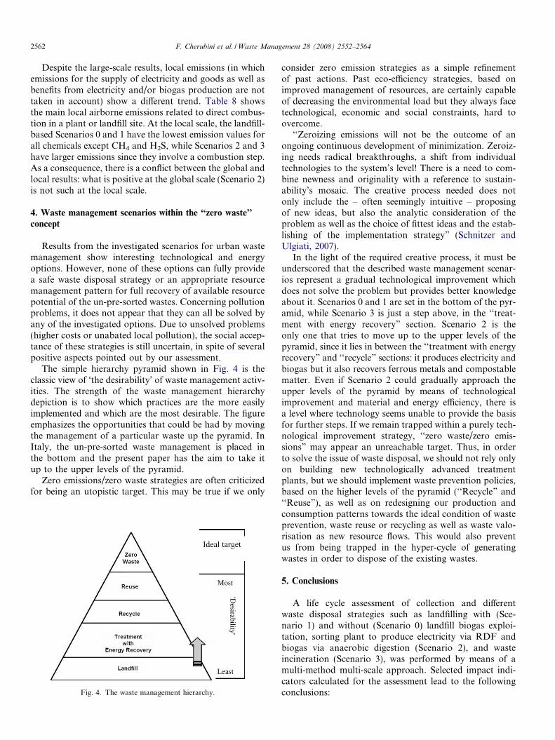
The simple hierarchy pyramid shown in Fig. 4 is theclassic view of ‘the desirability’ of waste management activ-ities. The strength of the waste management hierarchydepiction is to show which practices are the more easilyimplemented and which are the most desirable. The figureemphasizes the opportunities that could be had by movingthe management of a particular waste up the pyramid. InItaly, the un-pre-sorted waste management is placed inthe bottom and the present paper has the aim to take itup to the upper levels of the pyramid.

Zero emissions/zero waste strategies are often criticizedfor being an utopistic target. This may be true if we only

Fig. 4. The waste management hierarchy.

consider zero emission strategies as a simple refinementof past actions. Past eco-efficiency strategies, based onimproved management of resources, are certainly capableof decreasing the environmental load but they always facetechnological, economic and social constraints, hard toovercome.

‘‘Zeroizing emissions will not be the outcome of anongoing continuous development of minimization. Zeroiz-ing needs radical breakthroughs, a shift from individualtechnologies to the system’s level! There is a need to com-bine newness and originality with a reference to sustain-ability’s mosaic. The creative process needed does notonly include the – often seemingly intuitive – proposingof new ideas, but also the analytic consideration of theproblem as well as the choice of fittest ideas and the estab-lishing of the implementation strategy” (Schnitzer andUlgiati, 2007).

In the light of the required creative process, it must beunderscored that the described waste management scenar-ios represent a gradual technological improvement whichdoes not solve the problem but provides better knowledgeabout it. Scenarios 0 and 1 are set in the bottom of the pyr-amid, while Scenario 3 is just a step above, in the ‘‘treat-ment with energy recovery” section. Scenario 2 is theonly one that tries to move up to the upper levels of thepyramid, since it lies in between the ‘‘treatment with energyrecovery” and ‘‘recycle” sections: it produces electricity andbiogas but it also recovers ferrous metals and compostablematter. Even if Scenario 2 could gradually approach theupper levels of the pyramid by means of technologicalimprovement and material and energy efficiency, there isa level where technology seems unable to provide the basisfor further steps. If we remain trapped within a purely tech-nological improvement strategy, ‘‘zero waste/zero emis-sions” may appear an unreachable target. Thus, in orderto solve the issue of waste disposal, we should not rely onlyon building new technologically advanced treatmentplants, but we should implement waste prevention policies,based on the higher levels of the pyramid (‘‘Recycle” and‘‘Reuse”), as well as on redesigning our production andconsumption patterns towards the ideal condition of wasteprevention, waste reuse or recycling as well as waste valo-risation as new resource flows. This would also preventus from being trapped in the hyper-cycle of generatingwastes in order to dispose of the existing wastes.

5. Conclusions

A life cycle assessment of collection and differentwaste disposal strategies such as landfilling with (Sce-nario 1) and without (Scenario 0) landfill biogas exploi-tation, sorting plant to produce electricity via RDF andbiogas via anaerobic digestion (Scenario 2), and wasteincineration (Scenario 3), was performed by means of amulti-method multi-scale approach. Selected impact indi-cators calculated for the assessment lead to the followingconclusions:

F. Cherubini et al. / Waste Management 28 (2008) 2552–2564 2563

� Material flow accounting: The disposal of 1 g of wasterequires the production of about 0.3 g of further wasteas abiotic matter (the case studies range between0.24 gab of Scenario 0 to 0.36 gab of Scenario 3). Thiscalls for waste prevention policies in order to stop suchan additional cycle of waste production. Furthermore,none of the selected scenarios are able to completelyavoid the landfill, although in Scenarios 2 and 3 a reduc-tion up to 80% can be achieved, together with a changein waste composition.� Gross energy requirement: The scenarios able to mini-

mize the landfill (2 and 3) require a 20% increase of fossilenergy consumption for the disposal of waste. However,they can provide a consistent energy output that, in Sce-nario 2, could meet 15.5% of the Rome electricaldemand and 8.2% of the natural gas consumption(replaced by the upgraded biogas).� Emergy synthesis: The main result pointed out by the

emergy synthesis is that recycling is a rewarding prac-tice: the electricity production from waste combustionrequires less environmental support than hydropower.� Global and local emissions: Landfilling is the most pollut-

ing waste management option (concerning GWP, APand EP) at the global scale, since it is strongly affectedby many different emissions (CH4, H2S, HCl, N and Pinorganic compounds. . .) originated from the anaerobiccondition within the system. Furthermore, a landfillneeds to be monitored for a relatively long time periodin order to minimize its environmental impact. Never-theless, a conflict arises when local emissions areassessed, because Scenarios 2 and 3 – in spite of theirlarge-scale benefits – show the highest emissions at theplant scale.

An overall interpretation of these indicators suggests thelandfill systems (Scenarios 0 and 1) as the worst waste man-agement options. Results also show that a sorting plantcoupled with electricity and biogas production (Scenario2) is very likely to be the best option for waste manage-ment, despite the non-negligible problem of local emissions(NOx, PM10, heavy metals, HPA, among others). Further-more, in Scenario 2 and, to a smaller extent, Scenario 3, anon-negligible amount of energy becomes available, inspite of an increase of fossil fuel energy input of about20%, while waste residues to be landfilled are minimizedand inerted. Therefore, if we truly have to choose onlyamong the assessed options, even the incineration alterna-tive (Scenario 3) would appear to be better than landfilling(Scenarios 0 and 1), also from an environmental impactpoint of view.

However, none of the investigated scenarios are able tocompletely avoid the construction of a landfill. This aspecturgently calls for a breakthrough improvement: finding aconvenient way for reuse of bottom and fly ashes whichare now delivered to the landfill.

If environmental problems must be solved step by step(due to technological, economic and social constraints),

achieving ‘‘Reuse” and approaching the ideal target of zeroemissions may require that we have to pass through thelower levels of the pyramid of Fig. 4 (and then Scenario2 appears as the most suitable among the analysedoptions), in order to acquire experience, knowledge, under-standing and organization. The way this can be reached isby far a complex problem, the solution of which cannot beobtained only by means of a technological improvement,but also requires the involvement of concerned entrepre-neurs and consumers towards designing new patterns ofsustainable production and consumption.

References

AMA, 2003. Environmental Report. Available on the web on <www.ama-

roma.it> (in Italian).

APAT, Italian Agency for Environmental Protection and Technical

Services, 1999. Inventory of airborne emissions in atmosphere,

(CORINAIR-IPCC). Available on the web-site <www.apat.gov> (in

Italian).

Arena, U., Mastellone, M.L., Perugini, F., 2003. The environmental

performance of alternative solid waste management options: a life

cycle assessment study. Chemical Engineering Journal 96, 207–222.

Bargigli, S., Raugei, M., Ulgiati, S., 2005. Mass flow analysis and mass-

based indicators. In: Jorgensen, Sven E., Costanza, Robert, Xu, Fu-

Liu (Eds.), Handbook of Ecological Indicators for Assessment of

Ecosystem Health. CRC Press, pp. 353–378.

Berglund, M., Borjesson, P., 2006. Assessment of energy performance in

the life-cycle of biogas production. Biomass and Bioenergy 30, 254–

266.

Bjorklund, J., Geber, U., Rydberg, T., 2001. Emergy analysis of municipal

wastewater treatment and generation of electricity by digestion of

sewage sludge. Resources, Conservation and Recycling 31, 293–316.

Brown, M.T., Hall, C.A.S., 2004. Through the MACROSCOPE: the

legacy of H.T. Odum. An H.T. Odum Primer 178 (1–2), 201–213,

Special Issue of Ecological Modelling.

Brown, M.T., Ulgiati, S., 2004. Energy analysis and environmental

accounting. In: Cleveland, C. (Ed.), Encyclopedia of Energy. Aca-

demic Press/Elsevier, Oxford, UK, pp. 329–354.

Caputo, A.C., Pelagagge, P.M., 2002. RDF production plants: I. Design

and costs. Applied Thermal Engineering 22, 423–437.

Clift, R., Doig, A., Finnveden, G., 2000. The application of life cycle

assessment to integrated waste management. Part 1. Methodology.

Transactions of the Institute of Chemical Engineers 78 (B), 279–287.

Consonni, S., Giugliano, M., Grosso, M., 2005. Alternative strategies for

energy recovery from municipal solid waste Part B: Emission and cost

estimates. Waste Management 25, 137–148.

Conte, I., 2001. La produzione di energia dal biogas della discarica Basse

di Stura. Energy Manager Amiat S.p.A., Technical Report (in Italian).

EPA document, 1996. Compilation of air pollutant emission factors, vol.

I, fifth ed. point sources AP-42.

Frischknecht, R., Jungbluth, N., et al., 2003. Implementation of life cycle

impact assessment methods. Final Report ecoinvent 2000, Swiss

Centre for LCI. Duebendorf, CH.

Gravitis, J., Suzuki, M., 1999. From 3R to 4R approach and from oil

refinery to biorefinery. In: Proc. IV Intern. Congress on Energy,

Environment and Technological Innovation, vol. 1. Rome, Italy,

September 20–24, 1999, pp. 695–700.

Herendeen, R.A., 1998. Embodied Energy, embodied everything. . .now

what? In: Ulgiati, S. et al. (Eds.), Advances in Energy Studies. Energy

Flows in Ecology and Economy. Musis Publisher, Roma, Italy, pp.

13–48.

Hinterberger, F., Stiller, H., 1998. Energy and material flows. In: Ulgiati,

S. et al. (Eds.), Advances in Energy Studies. Energy Flows in Ecology

and Economy. Musis Publisher, Roma-Italy, pp. 275–286.

2564 F. Cherubini et al. / Waste Management 28 (2008) 2552–2564

IFIAS, International Federation of Institutes for Advanced Study, 1974.

In: Slesser, M., (Ed.), Energy analysis workshop on methodology and

conventions. Report IFIAS No. 89, Stockholm.

ISO (International Organization for Standardization) 14040, 1997. Envi-

ronmental Management – Life Cycle Assessment. Part 1. Principles

and Framework, Geneva, CH.

Khan, F.I., Sadiq, R., Husain, T., 2002. GreenPro-I: a risk-based life cycle

assessment and decision-making. Environmental Modelling and Soft-

ware 17, 669–692.

Kohl, A.L., Nielsen, R.B., 1997. Gas Purification. Gulf Publishing

Company, Houston, Texas.

Kylefors, K., 2003. Evaluation of leachate composition by multivariate data

analysis (MVDA). Journal of Environmental Management 68, 367–376.

LCA, 1997. A guide to approaches, experiences and information source,

Environmental Issue Series No. 6, European Environmental Agency.

Nielsen, P.H., Hauschild, M., 1998. Product specific emissions from

municipal solid waste landfills. Part I. Landfill model. International

Journal of LCA 3, 158–168.

Odum, H.T., 1988. Self-organization, transformity, and information.

Science 242, 1132–1139.

Odum, H.T., 1996. Environmental accounting. Energy and Environmental

Decision Making. John Wiley & Sons, N.Y., ISBN 0-471-11442-1, pp. 370.

Pauli, G., 1998. Upsizing. The road to zero emissions. More Jobs, More

Income and No Pollution. Greenleaf Publishing.

Ruth, L.A., 1998. Energy from municipal solid waste: a comparison with

coal combustion technology. Progress in Energy and Combustion

Science 24, 545–564.

Schmidt-Bleek, F., 1993. MIPS re-visited. Fresenius Environmental

Bulletin 2, 407–412.

Schnitzer, H., Ulgiati, S. (Eds.), 2007. Zero emission techniques

and strategies. Special Issue of the Journal of Cleaner Production

15(13–14).

Schnitzer, H., Ulgiati, S. (Eds.), 2007b. Less bad is not good enough:

approaching zero emissions techniques and systems. Journal of

Cleaner Production, Special Issue on Zero Emission Techniques and

Strategies 15(13–14), pp. 1–5.

Statistical Yearbook of Rome – Annuario Statistico di Roma. 2003.

Department XVII, Statistical office, Roma. www.comune.roma.it/

uffstat/ (in Italian).

Sundqvist, J.O., Finnveden, G., Albertsson, A.C., Karlsson, S., Berend-

son, J., Hoglund, L.O., 1997. Life Cycle Assessment and Solid Waste.

AFRReport 173, AFR, Stockholm, Sweden.

Ulgiati, S., 2000. Energy, emergy and embodied exergy: diverging or

converging approaches? Proceedings of the First Biennial Emergy

Analysis Research Conference, vol. 15. UFL, Gainesville, FL, USA.

Ulgiati, S., Raugei, M., Bargigli, S., 2006. Overcoming the inadequacy of

single-criterion approaches to life cycle assessment. Ecological Mod-

elling 190, 432–442.

USEPA, 1995. Locating and Estimating Air Emissions from Sources of

Dioxins and Furans. Office of Air Quality Planning and Standards,

Research Triangle Park, NC.

White, P.R., Franke, M., Hindle, P., 1999. Integrated Solid Waste

Management – A Life Cycle Inventory. Aspen Publishers Inc./

Chapman & Hall, Gaithersburg, MD, USA/New York.