20 Int. J. Engineering Systems Modelling and Simulation, Vol. 1, No. 1, 2008

Copyright © 2008 Inderscience Enterprises Ltd.

Direct simulation of viscous flow in a wavy pipe using the lattice Boltzmann approach

Lian-Ping Wang* Department of Mechanical Engineering, University of Delaware, Newark, DE 19716-3140, USA E-mail: lwang@udel.edu *Corresponding author

Michael H. Du Schlumberger Reservoir Completions, Rosharon, Texas 77583-1590, USA E-mail: du2@slb.com

Abstract: Direct numerical simulation of three-dimensional (3D) viscous flow in a wavy pipe is performed using the lattice Boltzmann approach, to study 3D flow features in a curved pipe with nonuniform curvature. We first validate the lattice Boltzmann approach by simulating a transient flow in a straight pipe. In a wavy pipe, it is shown that the pressure gradient necessary to drive the flow depends more strongly on the flow Reynolds number, due to curvature – induced fluid inertial force and transverse secondary flows. The wavy pipe could provide a simple design for enhancing mixing and heat transfer in pipes.

Keywords: viscous flows in curved pipe; direct numerical simulation; Lattice Boltzmann Method; LBM; Görtler vortices; pressure loss; flow transition; frictional coefficient; mixing.

Reference to this paper should be made as follows: Wang, L-P. and Du, M.H. (2008) ‘Direct simulation of viscous flow in a wavy pipe using the lattice Boltzmann approach’, Int. J. Engineering Systems Modelling and Simulation, Vol. 1, No. 1, pp.20–29.

Biographical notes: L-P. Wang is an Associate Professor of Mechanical Engineering at the University of Delaware. He received his PhD in Mechanical Engineering from Washington State University, USA and his BSc in Engineering Mechanics from Zhejiang University, Hangzhou, China. He applies advanced simulation tools and theoretical methods to study multiphase flows and transport in engineering applications and environmental processes, as well as to modelling of complex industrial flows.

M.H. Du is a Technical Group Leader of Core Completions at Schlumberger Reservoir Completions (SRC). He received his PhD in Mechanical Engineering from Texas A&M University, USA and his MSc and BSc in Engineering Mechanics from Zhejiang University, Hangzhou, China. He has worked at SRC on technology developments including Downhole Testing, Artificial Lift, Flow Control, and Completion Accessories.

1 Introduction

Viscous fluids are routinely transported in hydraulic pipes of a variety of sizes and shapes (Berger et al., 1983). For example, in oil service equipment, a control line is used for operating hydraulic elements in the down hole assembly; a chemical injection line is used for delivering chemicals into the designated location in the oil well for chemical treatment. Hydraulic pipes can also be used to implement optic fibre in a Distributed Temperature Sensing (DTS) system by pumping fluid to carry the fibre into a pipe in the oil well, so that a continuous monitoring of temperature profile in the oil well is possible. Indeed, the circular Poiseuille flow in a straight pipe represents the best-known solution in fluid mechanics. For flow Reynolds numbers

less than about 2000, a steady laminar flow in a straight circular pipe has the well-known parabolic velocity profile, and in this simplest case the fluid inertial force is identically zero. More frequently, however, hydraulic pipes may be designed into different geometries, to accommodate for different applications. For example, the pipe may be shaped into a spiral, in order to compensate for extension and rotation of the equipment. In these applications, especially in the optic fibre application, the geometry with curvature of the hydraulic pipe significantly affects the performance of the system. Curved tubes are also encountered in biological systems (Pedley, 1980).

The presence of pipe axis curvature has two immediate effects on the flow characteristics. First, the flow is no longer unidirectional so the fluid inertial force must be

Direct simulation of viscous flow in a wavy pipe using the lattice Boltzmann approach 21

considered. Second, geometric curvature along the flow direction can lead to secondary flow such as Görtler vortices (Saric, 1994), even at low flow Reynolds numbers. These have long been realised in previous studies of steady and oscillatory flow in curved pipes or tubes, using a variety of analytical, numerical and experimental techniques (Berger et al., 1983; Pedley, 1980). Most previous studies, however, considered flow in curved pipes with a uniform axial curvature, such as helically-coiled tubes and toroidal tubes, and assumed that the curvature ratio, namely, the ratio of the pipe radius to the radius of curvature of the pipe axis, is small. Related studies of curved geometry include tube and channel bends (Pruvost et al., 2004; Schonfeld and Hardt, 2004). These studies showed a complex dependence of secondary flow on the curvature parameter and increased mixing and heat transfer compared to that of straight pipe (Berger et al., 1983; Kumar et al., 2006; Sharp et al., 1991).

In this paper, we are aimed at developing a general computational method for simulating flow in a curved pipe, with arbitrary non-uniform curvature and flow Reynolds numbers. As a first step to better understand the geometric effect of hydraulic pipes on the related processes, we consider viscous flows in a wavy pipe where the axis of the pipe is sinusoidal in shape. In the case of wavy pipes, the axis curvature is not uniform; an analytical solution is no longer feasible. The flow geometry is no longer simple for numerical solutions of the Navier–Stokes equation. To the authors’ knowledge, no direct numerical simulations of three-dimensional viscous flow in a wavy pipe have been attempted previously, although some related numerical studies have been conducted for viscous flows in a straight pipe with varying cross-sectional area, e.g., see Mahmud et al. (2001). We are also unaware of any systematic experimental studies on viscous flows in a wavy pipe. A direct simulation of the flow inside a wavy pipe provides a logical first step in addressing the pipe geometric effect on the Fibre-In-Liquid (FIL) flow for the optic fibre pumping process. The three-dimensional nature of viscous flow in a wavy pipe also implies enhanced mixing and heat transfer, relative to that of a straight pipe, making an in-depth understanding of such flow highly desirable.

This paper addresses mainly direct numerical simulation of three-dimensional viscous flow in a wavy pipe. The numerical simulation is accomplished by employing a mesoscopic computational approach known as the lattice Boltzmann method (LBM). The LBM approach is based on a kinetic formulation and could have certain advantages over the traditional Navier–Stokes based Computational Fluid Dynamics (CFD) (Chen and Doolen, 1998; Qian et al., 1992). The basic idea of LBM is to use a mesoscopic model based on the Boltzmann equation, but retaining the simplest discretised version just sufficient to reproduce the macroscopic Navier–Stokes equation. There are two drawbacks of LBM, when compared with Navier–Stokes based CFD: the first is that a larger number of variables (typically 15 or 19 particle distributions at a given lattice point in 3D) need to be solved; the second is a relative lack

of experience by the general fluid mechanics community in understanding the accuracy and reliability of the approach and related implementation issues. However, these drawbacks are outweighed by its tremendous computational advantages including:

• quasi-linear nature of the lattice Boltzmann equation

• ease of imposing no-slip boundary conditions on walls in complex geometry

• straightforward coding and parallelisation

• flexibilities in incorporating interfacial physics in multiphase flows.

For these reasons, LBM models capable of addressing thermal flows, flows through porous media, multiphase flows, electro-osmotic flows, and contact line, etc., have been proposed in recent years. Two international meetings1 are currently being held annually with a focus on LBM-related methods and their applications to engineering and industrial problems. In this work, we exploit these advantages particularly the ease of imposing boundary conditions on the wavy pipe wall. The current study builds on our related experience in solving viscous flows in complex geometries, using LBM, as documented in Wang and Afsharpoya (2006) and Gao et al. (2007).

As the first step, we focus our attention on three-dimensional, steady laminar flow in a wavy pipe. The methodology for simulating the flow will be described in some detail, followed by both qualitative and quantitative descriptions of the simulated flows in a wavy pipe. The flow Reynolds numbers treated in this paper are somewhat below these actually encountered in the optic fibre application. The path forward to extending the present work to turbulent flows in a wavy pipe will be briefly discussed in the Summary section.

2 Methodology

2.1 Construction of wavy pipe and fluid lattice nodes

Consider a three-dimensional viscous flow in a wavy pipe as shown in Figure 1. The flow is driven by a constant pressure gradient or a body force in the y direction. Initially the flow is at rest. The flow is solved until a steady-state condition is reached. In this study, the geometry of the pipe is set up by first defining a sinusoidal axis representing the centre line of the wavy pipe. The flow is directed mainly in the y direction. The axis of the pipe is aligned in the x–y plane. The surface of the wavy pipe is formed by a series of circles of radius R with centre located on the axis, oriented normal to the local tangential direction of the axis (Figure 1(a)). For simplicity of implementing the periodic boundary condition in the flow direction, the portion of the axis defined as

02 cos , 0, for 0c

c c cyx A z y L

Lπ ≡ = ≤ ≤

(1)

22 L-P. Wang and M.H. Du

is used to define the computational domain. The wavy pipe is then completely specified by the three parameters A0, R, and L. Or, alternatively by three parameters:

• the pipe radius R

• the offset ratio A0/R

• the normalised wavelength L/R.

The wavy pipe reduces to a straight pipe if A0/R → 0.

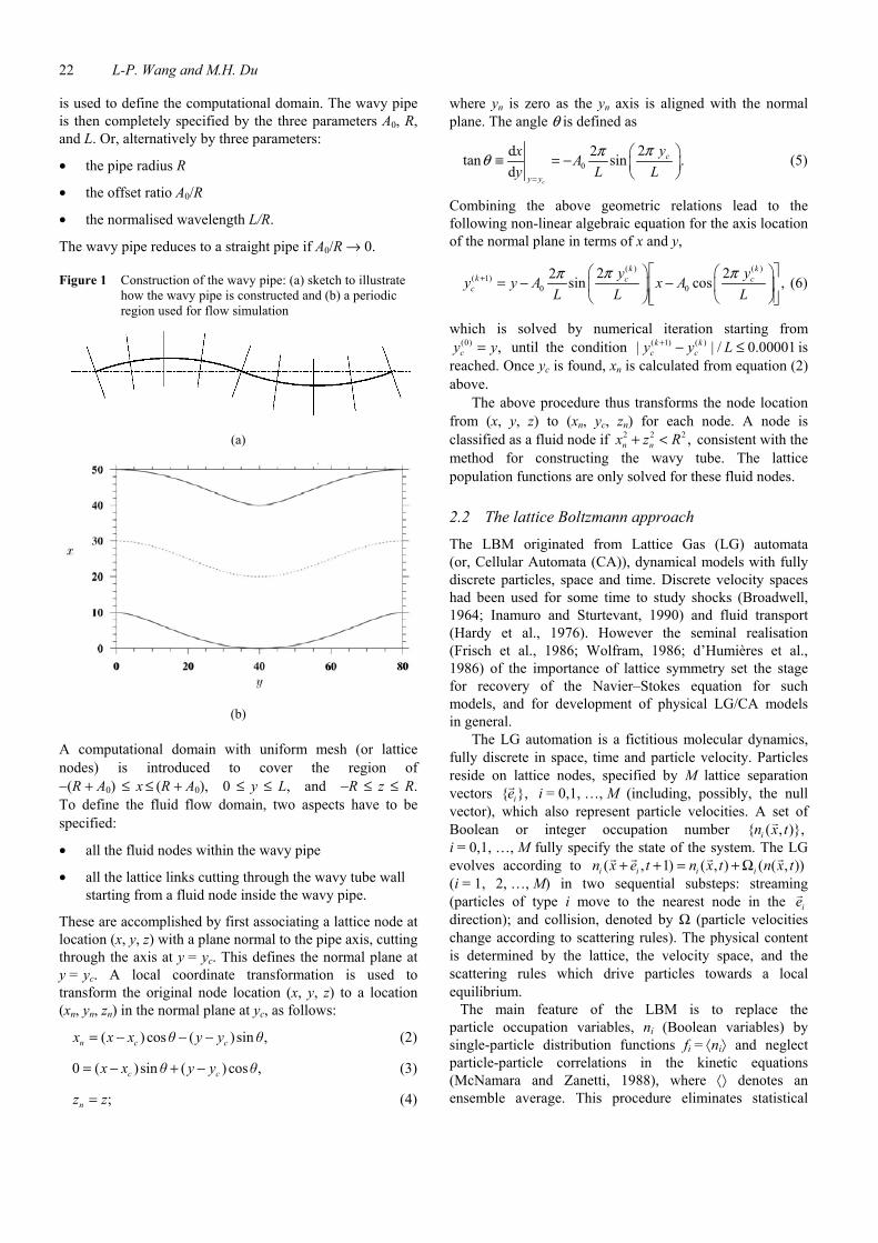
Figure 1 Construction of the wavy pipe: (a) sketch to illustrate how the wavy pipe is constructed and (b) a periodic region used for flow simulation

(a)

(b)

A computational domain with uniform mesh (or lattice nodes) is introduced to cover the region of −(R + A0) ≤ x ≤ (R + A0), 0 ≤ y ≤ L, and −R ≤ z ≤ R. To define the fluid flow domain, two aspects have to be specified:

• all the fluid nodes within the wavy pipe

• all the lattice links cutting through the wavy tube wall starting from a fluid node inside the wavy pipe.

These are accomplished by first associating a lattice node at location (x, y, z) with a plane normal to the pipe axis, cutting through the axis at y = yc. This defines the normal plane at y = yc. A local coordinate transformation is used to transform the original node location (x, y, z) to a location (xn, yn, zn) in the normal plane at yc, as follows:

( ) cos ( )sin ,n c cx x x θ y y θ= − − − (2)

0 ( )sin ( ) cos ,c cx x θ y y θ= − + − (3)

;nz z= (4)

where yn is zero as the yn axis is aligned with the normal plane. The angle θ is defined as

02 d 2tan sin .

dc

c

y y

yx Ay L L

ππθ=

≡ = −

(5)

Combining the above geometric relations lead to the following non-linear algebraic equation for the axis location of the normal plane in terms of x and y,

( ) ( )( 1)

0 02 2 2 sin cos ,

k kk c c

cy yy y A x A

L L Lπ ππ+

= − −

(6)

which is solved by numerical iteration starting from (0) ,cy y= until the condition ( 1) ( )| | / 0.00001k k

c cy y L+ − ≤ is reached. Once yc is found, xn is calculated from equation (2) above.

The above procedure thus transforms the node location from (x, y, z) to (xn, yc, zn) for each node. A node is classified as a fluid node if 2 2 2 ,n nx z R+ < consistent with the method for constructing the wavy tube. The lattice population functions are only solved for these fluid nodes.

2.2 The lattice Boltzmann approach

The LBM originated from Lattice Gas (LG) automata (or, Cellular Automata (CA)), dynamical models with fully discrete particles, space and time. Discrete velocity spaces had been used for some time to study shocks (Broadwell, 1964; Inamuro and Sturtevant, 1990) and fluid transport (Hardy et al., 1976). However the seminal realisation (Frisch et al., 1986; Wolfram, 1986; d’Humières et al., 1986) of the importance of lattice symmetry set the stage for recovery of the Navier–Stokes equation for such models, and for development of physical LG/CA models in general.

The LG automation is a fictitious molecular dynamics, fully discrete in space, time and particle velocity. Particles reside on lattice nodes, specified by M lattice separation vectors ,ie i = 0,1, …, M (including, possibly, the null vector), which also represent particle velocities. A set of Boolean or integer occupation number ( , ),in x t i = 0,1, …, M fully specify the state of the system. The LG evolves according to ( , 1) ( , ) ( ( , ))i i i in x e t n x t n x t+ + = + Ω (i = 1, 2, …, M) in two sequential substeps: streaming (particles of type i move to the nearest node in the ie direction); and collision, denoted by Ω (particle velocities change according to scattering rules). The physical content is determined by the lattice, the velocity space, and the scattering rules which drive particles towards a local equilibrium.

The main feature of the LBM is to replace the particle occupation variables, ni (Boolean variables) by single-particle distribution functions fi = ⟨ni⟩ and neglect particle-particle correlations in the kinetic equations (McNamara and Zanetti, 1988), where ⟨⟩ denotes an ensemble average. This procedure eliminates statistical

Direct simulation of viscous flow in a wavy pipe using the lattice Boltzmann approach 23

noise in the LG, while retaining advantages of locality which are essential to parallelism.

In the LBM approach, the lattice-Boltzmann equation for the distribution function fi of the mesoscopic particle with velocity ie

( )1( , ) ( , ) ( , ) ( , )

( , )

eqi i t t i i i

i

f x e t f x t f x t f x t

x t

δ δτψ

+ + − = − −

+ (7)

is solved with a prescribed forcing field ψi designed to model the driving pressure gradient or body force. In the above, the single timescale BGK collision operator (Bhatnagar et al., 1954; Chen et al., 1992; Qian et al., 1992) is adopted for its simplicity and computational efficiency.

In this work, ψi is specified as 2/ ,i i i sW e F cψ = ⋅ where F is the macroscopic force per unit mass acting on the fluid. The D3Q19 model (Qian et al., 1992) is used with the particle velocities: 0 (0,0,0),e = 1,2 ( 1,0,0),e = ±

3,4 (0, 1, 0),e = ± 5,6 (0,0, 1),e = ± 7,8,9,10 ( 1, 1, 0),e = ± ± 11,12,13,14 ( 1, 0, 1),e = ± ± and 15,16,17,18 (0, 1, 1).e = ± ± The

equilibrium distribution function is given as 2

( ) 0 02 4

: ( I)( , ) ,

2eq i i i s

i is s

e u uu e e cf x t W

c cρ ρρ

⋅ −= + +

(8)

where wi with i = 0, 1, 2, …, 18 are the weights and are equal to 1/3, 1/18, and 1/36, respectively, for particle with speeds of 0, 1, and 2; the sound speed cs is 1/ 3, and I ≡ δij is the second-order identity tensor. The mean density ρ0 is set to 1.0. The macroscopic hydrodynamic variables are computed as

20 s, , ,i i i

i i

f u f e p cρ ρ ρ= = =∑ ∑ (9)

where ρ, u , and p are the fluid density fluctuation (the local fluid density is ρ0 + ρ), velocity, and pressure, respectively. The above form of the equilibrium distribution was suggested by He and Luo (1997a) to best model the incompressible Navier–Stokes equation governing the macroscopic variables u and p. The fluid kinematic viscosity is related to the relaxation time by ν = (τ – 0.5)/3.

The lattice Boltzmann equation can also be derived directly from the Boltzmann equation (He and Luo, 1997b), thus may be viewed as a minimal or optimum mesoscopic model for the macroscopic Navier–Stokes equation. Hou et al. (1995) provided a detailed derivation that shows how the Navier–Stokes equations can be recovered from the lattice Boltzmann equation by using the Chapman–Enskog expansion procedure of kinetic theory. They also explained how the equilibrium distribution is obtained to guarantee that the requirements of isotropy, Galilean-invariance, and velocity-independent pressure are satisfied. Unlike most CFD methods that are based on direct discretisations of the second-order non-linear Navier–Stokes equations, the Boltzmann equation is a first-order linear equation with local non-linearity in the collision term only. This gives

LBM a great computational advantage. For further historical background and applications of LBM, the readers are referred to the review papers by Chen and Doolen (1998) and Yu et al. (2003).

In this study, a uniform lattice is used to cover the computational domain. The first and the last layers of lattice nodes in the y direction are placed half-lattice unit away from inlet and outlet to facilitate the implementation of the periodic inlet-outlet boundary condition.

The key implementation issue here is the treatment of the no-slip boundary condition on the wavy wall surface. For each lattice node near the wavy wall, we identify all links moving into the wall and their relative boundary-cutting location, namely, the percentage (α) of a link located inside the fluid region (e.g., see Lallemand and Luo, 2003). Since the wall is fixed, this information is pre-processed before the flow evolution and saved as one-dimensional arrays for memory efficiency. Before the streaming step, the missing populations are properly interpolated in terms of α and two populations lying before and after the path of the missing population (Yu et al., 2003; Lallemand and Luo, 2003). These are saved on auxiliary lattice nodes in buffer layers surrounding the fluid domain. For results in this paper, we used the first-order interpolation based on two known populations, and found that the results are quite similar to the second-order interpolation based on three nodes (Lallemand and Luo, 2003). All lattice nodes lying outside the wall surface (including the wall interface) are excluded from LBE evolution, and their velocities are simply set to zero. As a validation check, the total mass for the fluid nodes (excluding the fluid-solid interface nodes) is computed and found to remain as a constant as time is advanced.

We also implemented the generalised lattice Boltzmann equation or the Multiple-Relaxation-Time (MRT) model as presented in d’Humières et al. (2002) and Lallemand and Luo (2003). The MRT has been shown to improve numerical stability so flows at higher Reynolds numbers can be simulated. Most results presented here are based on the MRT collision model of d’Humières et al. (2002).

3 Results

3.1 Validation for transient flow in a straight pipe

To validate the three-dimensional LBM code, we first simulate a transient flow in a straight pipe. The flow is assumed to be at rest at t = 0 and is driven by a constant pressure gradient (dp/dy = constant). The analytical solution for the time-dependent velocity profile can be written in terms of the Bessel function as (Brereton and Jiang, 2005).

( )( )

2

220

2 3 21 1

dv ( , )4 d

8 / 1 exp ,n n

n n n

R pr ty

J r R trR J R

µλ λ ν

λ λ

∞

=

= −

−× − −

∑ (10)

24 L-P. Wang and M.H. Du

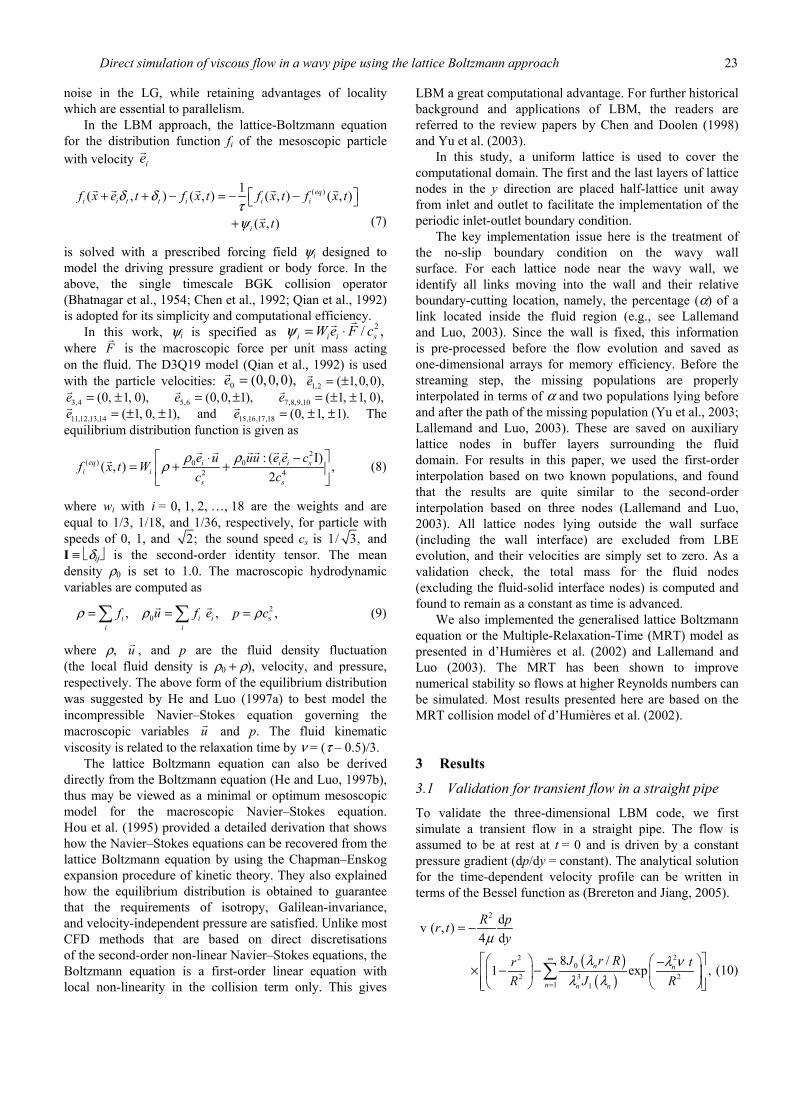
where Ji is the Bessel function of the first kind, λn are roots of J0, and µ = ρ0ν is the fluid viscosity. Figure 2 compares the axial velocity distribution obtained from LBM with the analytical solution at four different times. The steady-state centreline velocity V0 = −(R2/4µ)dp/dy is used to normalise the velocity. The radius of the pipe is set to 30 lattice units. The relaxation time is set to 1.0 giving a kinematic viscosity of 1/6. The steady-state centreline velocity is set to 0.1. Therefore, the flow Reynolds number based on the steady-state mean flow speed is 18. For each time in Figure 2, the streamwise velocities at all 2828 lattice points in the inlet plane are plotted (note that the cross-sectional area is πR2 = 2827.4). The LBM data match quite precisely the analytical solution at all times.

Figure 2 Comparison of LBE solution with analytical solution for a transient flow in a straight pipe. The normalised times from bottom to top are νt/R2 = 0.185, 0.370, 0.555, 0.740, respectively. The plus symbols denote the LBM data and the dash lines show the analytical solution, equation (10). The top shows all fluid lattice points, while the bottom is an enlarged view near the wall

The bottom panel of Figure 2 is an enlarged view near the wall region. It is remarkable that the velocities at all lattice nodes match the theoretical curves in the near-wall region, showing the accuracy and reliability of the LBM method.

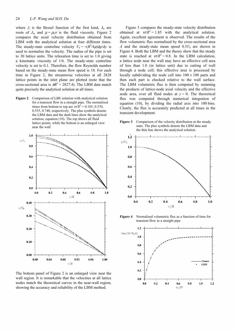
Figure 3 compares the steady-state velocity distribution obtained at νt/R2 = 1.85 with the analytical solution. Again, excellent agreement is observed. The results of the flow volumetric flux normalised by the cross-sectional area A and the steady-state mean speed 0.5V0 are shown in Figure 4. Both the LBM and the theory show that the steady state is reached at νt/R2 = 0.8. In the LBM calculation, a lattice node near the wall may have an effective cell area of less than 1.0 (in lattice unit) due to cutting of wall through a node cell; this effective area is processed by locally subdividing the node cell into 100 × 100 parts and then each part is checked relative to the wall surface. The LBM volumetric flux is then computed by summing the products of lattice-node axial velocity and the effective node area, over all fluid nodes at y = 0. The theoretical flux was computed through numerical integration of equation (10), by dividing the radial axis into 100 bins. Clearly, the flux is accurately predicted at all times in the transient development.

Figure 3 Comparison of the velocity distribution at the steady state. The plus symbols denote the LBM data and the thin line shows the analytical solution

Figure 4 Normalised volumetric flux as a function of time for transient flow in a straight pipe

Direct simulation of viscous flow in a wavy pipe using the lattice Boltzmann approach 25

The case study above is for a given flow Reynolds number (Re = 18). Several other flow Reynolds numbers (Re = 120 and Re = 400) were also simulated, yielding the same excellent agreement with the theoretical prediction. The above comparisons show that both local distributions and integral properties of the transient flow have been accurately reproduced by the LBM method.

3.2 Viscous flow in a wavy pipe

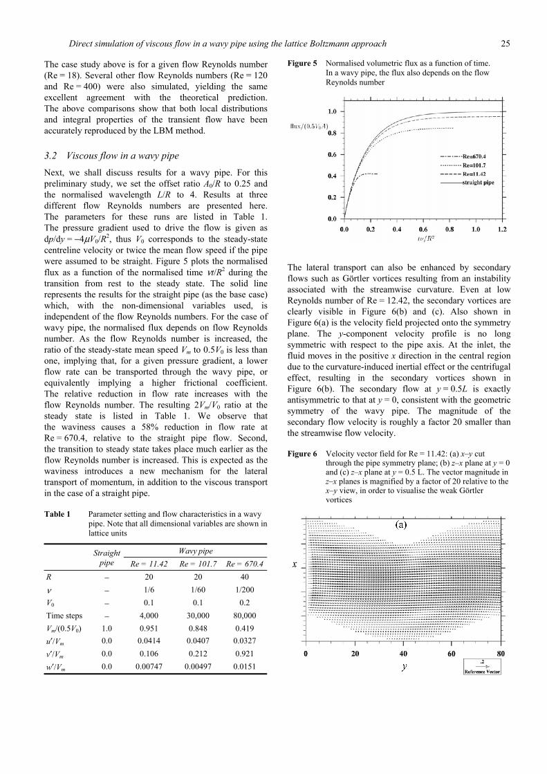
Next, we shall discuss results for a wavy pipe. For this preliminary study, we set the offset ratio A0/R to 0.25 and the normalised wavelength L/R to 4. Results at three different flow Reynolds numbers are presented here. The parameters for these runs are listed in Table 1. The pressure gradient used to drive the flow is given as dp/dy = −4µV0/R2, thus V0 corresponds to the steady-state centreline velocity or twice the mean flow speed if the pipe were assumed to be straight. Figure 5 plots the normalised flux as a function of the normalised time νt/R2 during the transition from rest to the steady state. The solid line represents the results for the straight pipe (as the base case) which, with the non-dimensional variables used, is independent of the flow Reynolds numbers. For the case of wavy pipe, the normalised flux depends on flow Reynolds number. As the flow Reynolds number is increased, the ratio of the steady-state mean speed Vm to 0.5V0 is less than one, implying that, for a given pressure gradient, a lower flow rate can be transported through the wavy pipe, or equivalently implying a higher frictional coefficient. The relative reduction in flow rate increases with the flow Reynolds number. The resulting 2Vm/V0 ratio at the steady state is listed in Table 1. We observe that the waviness causes a 58% reduction in flow rate at Re = 670.4, relative to the straight pipe flow. Second, the transition to steady state takes place much earlier as the flow Reynolds number is increased. This is expected as the waviness introduces a new mechanism for the lateral transport of momentum, in addition to the viscous transport in the case of a straight pipe.

Table 1 Parameter setting and flow characteristics in a wavy pipe. Note that all dimensional variables are shown in lattice units

Wavy pipe Straight pipe Re = 11.42 Re = 101.7 Re = 670.4

R − 20 20 40

ν − 1/6 1/60 1/200 V0 − 0.1 0.1 0.2 Time steps − 4,000 30,000 80,000 Vm/(0.5V0) 1.0 0.951 0.848 0.419 u′/Vm 0.0 0.0414 0.0407 0.0327 v′/Vm 0.0 0.106 0.212 0.921 w′/Vm 0.0 0.00747 0.00497 0.0151

Figure 5 Normalised volumetric flux as a function of time. In a wavy pipe, the flux also depends on the flow Reynolds number

The lateral transport can also be enhanced by secondary flows such as Görtler vortices resulting from an instability associated with the streamwise curvature. Even at low Reynolds number of Re = 12.42, the secondary vortices are clearly visible in Figure 6(b) and (c). Also shown in Figure 6(a) is the velocity field projected onto the symmetry plane. The y-component velocity profile is no long symmetric with respect to the pipe axis. At the inlet, the fluid moves in the positive x direction in the central region due to the curvature-induced inertial effect or the centrifugal effect, resulting in the secondary vortices shown in Figure 6(b). The secondary flow at y = 0.5L is exactly antisymmetric to that at y = 0, consistent with the geometric symmetry of the wavy pipe. The magnitude of the secondary flow velocity is roughly a factor 20 smaller than the streamwise flow velocity.

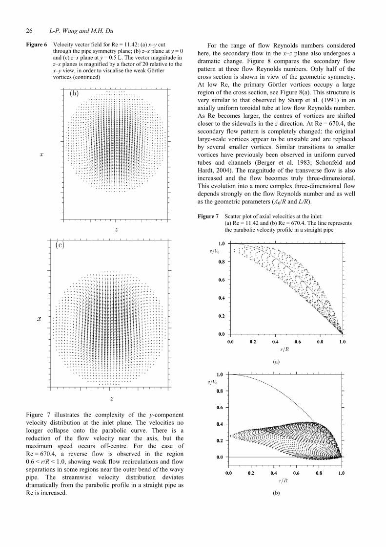
Figure 6 Velocity vector field for Re = 11.42: (a) x–y cut through the pipe symmetry plane; (b) z–x plane at y = 0 and (c) z–x plane at y = 0.5 L. The vector magnitude in z–x planes is magnified by a factor of 20 relative to the x–y view, in order to visualise the weak Görtler vortices

26 L-P. Wang and M.H. Du

Figure 6 Velocity vector field for Re = 11.42: (a) x–y cut through the pipe symmetry plane; (b) z–x plane at y = 0 and (c) z–x plane at y = 0.5 L. The vector magnitude in z–x planes is magnified by a factor of 20 relative to the x–y view, in order to visualise the weak Görtler vortices (continued)

Figure 7 illustrates the complexity of the y-component velocity distribution at the inlet plane. The velocities no longer collapse onto the parabolic curve. There is a reduction of the flow velocity near the axis, but the maximum speed occurs off-centre. For the case of Re = 670.4, a reverse flow is observed in the region 0.6 < r/R < 1.0, showing weak flow recirculations and flow separations in some regions near the outer bend of the wavy pipe. The streamwise velocity distribution deviates dramatically from the parabolic profile in a straight pipe as Re is increased.

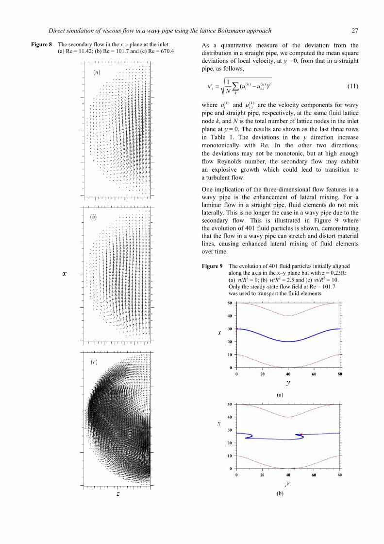
For the range of flow Reynolds numbers considered here, the secondary flow in the x–z plane also undergoes a dramatic change. Figure 8 compares the secondary flow pattern at three flow Reynolds numbers. Only half of the cross section is shown in view of the geometric symmetry. At low Re, the primary Görtler vortices occupy a large region of the cross section, see Figure 8(a). This structure is very similar to that observed by Sharp et al. (1991) in an axially uniform toroidal tube at low flow Reynolds number. As Re becomes larger, the centres of vortices are shifted closer to the sidewalls in the z direction. At Re = 670.4, the secondary flow pattern is completely changed: the original large-scale vortices appear to be unstable and are replaced by several smaller vortices. Similar transitions to smaller vortices have previously been observed in uniform curved tubes and channels (Berger et al. 1983; Schonfeld and Hardt, 2004). The magnitude of the transverse flow is also increased and the flow becomes truly three-dimensional. This evolution into a more complex three-dimensional flow depends strongly on the flow Reynolds number and as well as the geometric parameters (A0/R and L/R).

Figure 7 Scatter plot of axial velocities at the inlet: (a) Re = 11.42 and (b) Re = 670.4. The line represents the parabolic velocity profile in a straight pipe

(a)

(b)

Direct simulation of viscous flow in a wavy pipe using the lattice Boltzmann approach 27

Figure 8 The secondary flow in the x–z plane at the inlet: (a) Re = 11.42; (b) Re = 101.7 and (c) Re = 670.4

As a quantitative measure of the deviation from the distribution in a straight pipe, we computed the mean square deviations of local velocity, at y = 0, from that in a straight pipe, as follows,

( ) ( ) 2,

1 ( )k ki i s i

ku' u u

N= −∑ (11)

where ( )kiu and ( )

,k

s iu are the velocity components for wavy pipe and straight pipe, respectively, at the same fluid lattice node k, and N is the total number of lattice nodes in the inlet plane at y = 0. The results are shown as the last three rows in Table 1. The deviations in the y direction increase monotonically with Re. In the other two directions, the deviations may not be monotonic, but at high enough flow Reynolds number, the secondary flow may exhibit an explosive growth which could lead to transition to a turbulent flow.

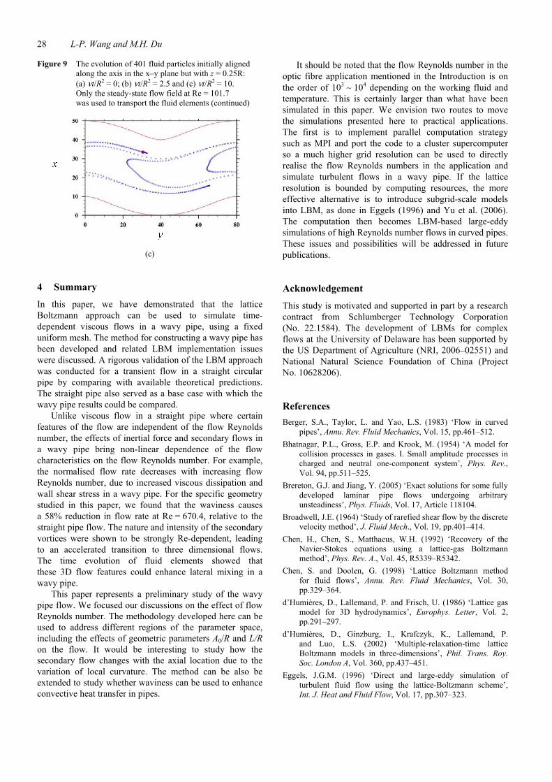
One implication of the three-dimensional flow features in a wavy pipe is the enhancement of lateral mixing. For a laminar flow in a straight pipe, fluid elements do not mix laterally. This is no longer the case in a wavy pipe due to the secondary flow. This is illustrated in Figure 9 where the evolution of 401 fluid particles is shown, demonstrating that the flow in a wavy pipe can stretch and distort material lines, causing enhanced lateral mixing of fluid elements over time.

Figure 9 The evolution of 401 fluid particles initially aligned along the axis in the x–y plane but with z = 0.25R: (a) νt/R2 = 0; (b) νt/R2 = 2.5 and (c) νt/R2 = 10. Only the steady-state flow field at Re = 101.7 was used to transport the fluid elements

(a)

(b)

28 L-P. Wang and M.H. Du

Figure 9 The evolution of 401 fluid particles initially aligned along the axis in the x–y plane but with z = 0.25R: (a) νt/R2 = 0; (b) νt/R2 = 2.5 and (c) νt/R2 = 10. Only the steady-state flow field at Re = 101.7 was used to transport the fluid elements (continued)

(c)

4 Summary

In this paper, we have demonstrated that the lattice Boltzmann approach can be used to simulate time-dependent viscous flows in a wavy pipe, using a fixed uniform mesh. The method for constructing a wavy pipe has been developed and related LBM implementation issues were discussed. A rigorous validation of the LBM approach was conducted for a transient flow in a straight circular pipe by comparing with available theoretical predictions. The straight pipe also served as a base case with which the wavy pipe results could be compared.

Unlike viscous flow in a straight pipe where certain features of the flow are independent of the flow Reynolds number, the effects of inertial force and secondary flows in a wavy pipe bring non-linear dependence of the flow characteristics on the flow Reynolds number. For example, the normalised flow rate decreases with increasing flow Reynolds number, due to increased viscous dissipation and wall shear stress in a wavy pipe. For the specific geometry studied in this paper, we found that the waviness causes a 58% reduction in flow rate at Re = 670.4, relative to the straight pipe flow. The nature and intensity of the secondary vortices were shown to be strongly Re-dependent, leading to an accelerated transition to three dimensional flows. The time evolution of fluid elements showed that these 3D flow features could enhance lateral mixing in a wavy pipe.

This paper represents a preliminary study of the wavy pipe flow. We focused our discussions on the effect of flow Reynolds number. The methodology developed here can be used to address different regions of the parameter space, including the effects of geometric parameters A0/R and L/R on the flow. It would be interesting to study how the secondary flow changes with the axial location due to the variation of local curvature. The method can be also be extended to study whether waviness can be used to enhance convective heat transfer in pipes.

It should be noted that the flow Reynolds number in the optic fibre application mentioned in the Introduction is on the order of 103 ∼ 104 depending on the working fluid and temperature. This is certainly larger than what have been simulated in this paper. We envision two routes to move the simulations presented here to practical applications. The first is to implement parallel computation strategy such as MPI and port the code to a cluster supercomputer so a much higher grid resolution can be used to directly realise the flow Reynolds numbers in the application and simulate turbulent flows in a wavy pipe. If the lattice resolution is bounded by computing resources, the more effective alternative is to introduce subgrid-scale models into LBM, as done in Eggels (1996) and Yu et al. (2006). The computation then becomes LBM-based large-eddy simulations of high Reynolds number flows in curved pipes. These issues and possibilities will be addressed in future publications.

Acknowledgement

This study is motivated and supported in part by a research contract from Schlumberger Technology Corporation (No. 22.1584). The development of LBMs for complex flows at the University of Delaware has been supported by the US Department of Agriculture (NRI, 2006–02551) and National Natural Science Foundation of China (Project No. 10628206).

References Berger, S.A., Taylor, L. and Yao, L.S. (1983) ‘Flow in curved

pipes’, Annu. Rev. Fluid Mechanics, Vol. 15, pp.461–512. Bhatnagar, P.L., Gross, E.P. and Krook, M. (1954) ‘A model for

collision processes in gases. I. Small amplitude processes in charged and neutral one-component system’, Phys. Rev., Vol. 94, pp.511–525.

Brereton, G.J. and Jiang, Y. (2005) ‘Exact solutions for some fully developed laminar pipe flows undergoing arbitrary unsteadiness’, Phys. Fluids, Vol. 17, Article 118104.

Broadwell, J.E. (1964) ‘Study of rarefied shear flow by the discrete velocity method’, J. Fluid Mech., Vol. 19, pp.401–414.

Chen, H., Chen, S., Matthaeus, W.H. (1992) ‘Recovery of the Navier-Stokes equations using a lattice-gas Boltzmann method’, Phys. Rev. A., Vol. 45, R5339–R5342.

Chen, S. and Doolen, G. (1998) ‘Lattice Boltzmann method for fluid flows’, Annu. Rev. Fluid Mechanics, Vol. 30, pp.329–364.

d’Humières, D., Lallemand, P. and Frisch, U. (1986) ‘Lattice gas model for 3D hydrodynamics’, Europhys. Letter, Vol. 2, pp.291–297.

d’Humières, D., Ginzburg, I., Krafczyk, K., Lallemand, P. and Luo, L.S. (2002) ‘Multiple-relaxation-time lattice Boltzmann models in three-dimensions’, Phil. Trans. Roy. Soc. London A, Vol. 360, pp.437–451.

Eggels, J.G.M. (1996) ‘Direct and large-eddy simulation of turbulent fluid flow using the lattice-Boltzmann scheme’, Int. J. Heat and Fluid Flow, Vol. 17, pp.307–323.

Direct simulation of viscous flow in a wavy pipe using the lattice Boltzmann approach 29

Frisch, U., Hasslacher, B. and Pomeau, Y. (1986) ‘Lattice gas automata for the Navier-Stokes equation’, Phys. Rev. Lett., Vol. 56, pp.1505–1508.

Gao, H., Han, J., Jin Y. and Wang, L-P. (2007) ‘Modeling microscale flow and colloid transport in saturated porous media’, Int. J. Computational Fluid Dynamics (accepted).

Hardy, J., de Pazzis, O. and Pomeau, Y. (1976) ‘Molecular dynamics of a classical lattice gas: transport properties and time correlation functions’, Phys. Rev. A., Vol. 13, pp.1949–1961.

He, X. and Luo, L-S. (1997a) ‘Lattice Boltzmann model for the incompressible Navier-Stokes equation’, J. Stat. Phys., Vol. 88, pp.927–944.

He, X. and Luo, L-S. (1997b) ‘Theory of lattice Boltzmann method: From the Boltzmann equation to the lattice Boltzmann equation’, Phys. Rev. E., Vol. 56, pp.6811–6817.

Hou, S.L., Zou, Q., Chen, S.Y., Doolen, G. and Cogley, A.C. (1995) ‘Simulation of cavity flow by the lattice Boltzmann method’, J. Comp. Phys., Vol. 118, No. 2, pp.329–347.

Inamuro, T. and Sturtevant, B. (1990) ‘Numerical study of discrete-velocity gases’, Phys. Fluids, Vol. 2: pp.2196–2203.

Kumar, V., Aggarwal, M., Nigam, K.D.P. (2006) ‘Mixing in curved tubes’, Chem. Eng. Sci., Vol. 61, pp.5742–5753.

Lallemand, P. and Luo, L-S. (2003) ‘Lattice Boltzmann method for moving boundaries’, J. Comp. Phys., Vol. 184, pp.406–421.

Mahmud, S., Sadrul Islam, A.K.M. and Das, P.K. (2001) ‘Numerical prediction of fluid flow and heat transfer in a wavy pipe’, J. Thermal Sci., Vol. 10, pp.133–147.

McNamara, G.R. and Zanetti, G. (1988) ‘Use of the Boltzmann equation to simulate lattice-gas automata’, Phys. Rev. Lett., Vol. 61, pp.2332–2335.

Pedley, J.T. (1980) The Fluid Mechanics of Large Blood Vessels, Cambridge University Press, Cambridge, pp.160–234.

Pruvost, J., Legrand, J. and Legentilhomme, P. (2004) ‘Numerical investigation of bend and torus flows, part I: effect of swirl motion on flow structure in U-bend’, Chem. Engr. Sci., Vol. 59, pp.3345–3357.

Qian, Y.H., Dhumieres, D. and Lallemand, P. (1992) ‘Lattice BGK models for Navier-Stokes equation’, Europhysics Letters, Vol. 17, pp.479–484.

Saric, W.S. (1994) ‘Görtler vortices’, Annu. Rev. Fluid Mech., Vol. 26, pp.379–409.

Schonfeld, F. and Hardt, S. (2004) ‘Simulation of helical flows in microchannels’, AICHE J., Vol. 50, pp.771–778.

Sharp, M.K., Kamm, R.D., Shapiro, A.H., Kimmel, E. and Karniadakis, G.E. (1991) ‘Dispersion in a curved tube during oscillatory flow’, J. Fluid Mech., Vol. 223, pp.537–563.

Wang, L-P. and Afsharpoya, B. (2006) ‘Modeling fluid flow in fuel cells using the lattice Boltzmann approach’, Mathematics and Computers in Simulation, Vol. 72, pp.242–248.

Wolfram, S. (1986) ‘Cellular automaton fluids. I. Basic theory’, J. Stat. Phys., Vol. 45, pp.471–526.

Yu, D., Mei, R., Luo, L-S. and Shyy, W. (2003) ‘Viscous flow computations with the method of lattice Boltzmann equation’, Progress in Aerospace Sci., Vol. 39, pp.329–367.

Yu, H., Luo, L.S. and Girimaji, S.S. (2006) ‘LES of turbulent square jet flow using an MRT lattice Boltzmann model’, Computers and Fluids, Vol.35, pp.957–965.

Note 1These two annual meetings are the International Conference for Mesoscopic Methods in Engineering and Science (see http://www.icmmes.org/index.php) and International Conference on the Discrete Simulation of Fluid Dynamics (see http://nanotech.ucalgary.ca/dsfd2007/).