Embed Size (px)
Citation preview
May 24, 1994
Dear Reader:
These Standard References for Geophysical Investigations, WSC-94-311, describe the various geophysical methodologies available for conducting environmental investigations. The intended use of this document is to provide the technical layperson with enough knowledge to determine which geophysical method or groups of methods would best be suited for a specific project data collection requirement. Standard References for Geophysical Investigations was developed to help ensure data used for environmental investigative purposes is valid and can be interpreted consistently by anyone assessing environmental conditions, including Department staff, consultants, drillers and firms performing these assessments.
Many people, from within and outside the Department, were involved in developing this technical document. These References represent the Department's current understanding of the art of geophysical investigations. We welcome any information on innovative field techniques, suggestions for updates, or comments. This document will be updated to reflect new information about emerging technologies as our resources permit.
These References are one of several initiatives the Department is undertaking to provide clear, practical guidance for those affected by Massachusetts environmental regulations. We hope that you find this document a valuable tool.
Very truly yours,
Thomas B. Powers Acting Commissioner

STANDARD REFERENCES FOR GEOPHYSICAL INVESTIGATIONS
#WSC 94-311
COMMONWEALTH OF MASSACHUSETTS
DEPARTMENT OF ENVIRONMENTAL PROTECTION
This document is dedicated with great affection to Dodie Brownlee. She was the first hydrologist in the Department of Environmental Quality Engineering (now the Department of Environmental Protection). Dodie worked tirelessly to protect and improve our environment.
Dodie Brownlee conceived and developed these Standard References for Geophysical Investigations. She worked on them until her death in the spring of 1990.
May her spirit of commitment and drive for excellence live on through all of us.

COMMONWEALTH OF MASSACHUSETTS
DEPARTMENT OF ENVIRONMENTAL PROTECTION
STANDARD REFERENCES FOR GEOPHYSICAL INVESTIGATIONS
SECTION 1.0 INTRODUCTION
Section 1.0Page i
November 1993
SECTION 1.0INTRODUCTION
TABLE OF CONTENTS
Section Title Page No.
1.0 INTRODUCTION..................................... 1
1.1 Document Structure............................... 21.2 Background Reference Materials................... 3
REFERENCES ................................................. 4

Section 1.0Page 1
November 1993
1.0 INTRODUCTION
A geophysical survey is an indirect method of determining the state of the subsurface in the survey area. By indirect, it is meant that the geophysical survey measures some physical property of the subsurface and uses the results to infer the material that caused it. Like a blind person trying to identify an object without the benefit of sight, the geophysicist cannot directly observe the subsurface but must instead rely on other, less direct methods of data collection to make his/her determination as to its state. Variations in the electrical field (applied and ambient), gravity and magnetic potentials, and seismic wave velocities, amplitudes and frequencies are systematically measured to infer the structure and composition of the subsurface soil, rocks and groundwater.
Many geophysical methods produce results which by themselves cannot provide a definitive characterization of subsurface conditions; however, by using a combination of geophysical techniques (each of which measures a different physical property of the earth), the geophysicist can often eliminate incorrect possibilities to arrive at a correct interpretation. As an example, a terrain conductivity survey (an electromagnetic survey method described in Section 6.0) conducted over a landfill will detect areas of high subsurface conductivity. These areas of high conductivity could be caused by disturbed soil (landfilled area), a conductive contaminant plume, buried aluminum, or buried ferrous metal (possibly buried drums). If the areas exhibiting high soil conductivity were subsequently surveyed with a magnetometer (Section 8.0), which is sensitive only to ferrous metals, then the areas containing the potential buried drums could be distinguished from the rest of the identified anomalies.
The usefulness of geophysical techniques for site characterization and the evaluation of contaminated sites has been well-established during the past two decades. Determination of depths to both bedrock and the water table are routinely performed. Geophysical techniques are also used with great success to locate buried metal objects (barrels, tanks, pipes, trucks), certain migrating contaminant plumes, debris-filled trenches, determine the integrity of "cut off" slurry trenches, and trace the migration of contaminants through fractured bedrock.
A geophysical survey can be designed to measure the physical properties of earth materials either in detail or as an average over relatively large areas. Depending on "sampling" frequency and the technique used, geophysical methods measure either the detailed or the averaged physical properties of materials for the points of observation. All methods are inherently subject to greater averaging and lower resolution as distances between sampling points increase.
Geophysical investigations in environmental studies are best used to:
Section 1.0Page 2
November 1993
o Characterize geologic conditions
o Determine the source and extent of contamination problems
o Optimize test pit and boring locations
In many cases, the proper application of a geophysical investigation adds significant information and reduces the costs necessary to acquire the information required to determine effective site remediation and cleanup. The correlation of geophysical data methods, with borehole geologic and sampling data will usually provide the most meaningful results.
One significant issue that cannot be fully explored in this document is that of cost effectiveness. Geophysical exploration techniques may seem exotic but they should be viewed simply as data collection tools similar to soil borings and test pits. The fact that a geophysical technique can be employed to answer a question is not by itself enough of a justification to use it. The project manager should always ask him/herself the question: What is the most cost effective way to collect the data I need? If needed data can be collected most cost effectively by test pitting, then test pitting should be employed. If, on the other hand, it is determined that a geophysical method is quicker and cheaper to collect needed data then the geophysical method should be employed. It should be noted that results of geophysical site investigations alone, rarely provide complete answers to the data requirements of an environmental investigation. An intrusive (e.g., soil boring) program is usually necessary to supplement a geophysical program. Results of the geophysical program, however, can minimize the number of borings necessary by optimizing their placement. In return, the borings provide important data which can be used to refine geophysical interpretations and results. Geophysical methods can provide accurate and inexpensive (in comparison with conventional intrusive techniques) measurements of average subsurface conditions over large areas, while borings provide detailed information for a limited area. A combined geophysical survey/boring program is therefore often the most cost-effective system for the complete analysis of site conditions.
1.1 Document Structure
This document has been divided into 11 sections and are as follows:
o 1.0 Introduction
o 2.0 Planning a Geophysical Investigation
o 3.0 Seismic Methods
o 4.0 Resistivity Methods
Section 1.0Page 3
November 1993
o 5.0 Self-Potential Method
o 6.0 Electromagnetic Induction Methods (EM)
o 7.0 Ground Penetrating Radar (GPR)
o 8.0 Magnetic Methods
o 9.0 Gravity Method
o 10.0 Borehole Geophysical Methods
o 11.0 Underwater Methods
Section 2.0 outlines a decision making process which can be used to determine the scope of a geophysical investigation. This section includes references to specific sections which cover the referenced techniques which are covered in greater detail in later sections. Sections 3.0 through 9.0 cover specific geophysical techniques indicated by the section title. Section 10.0 covers the suite of geophysical techniques which are commonly used in the investigation of subsurface conditions using soil borings and monitoring wells. Section 11.0 covers the marine geophysical techniques which could be applied to ocean, river, pond, or lake environments, if required.
1.2 Background Reference Materials
Texts that generally discuss the applicable geophysical techniques include Dobrin (1976), Telford et al. (1976), Mooney (1977), U.S. Army Corps of Engineers (1979), Grant and West (1965), and Griffiths and King (1981). A comprehensive discussion of geophysical methods and their application to groundwater problems is included in the 1985 Electric Power Research Institute's Groundwater Manual for the Electric Utility Industry, Volume 3, Groundwater Investigation and Mitigation Techniques, Section 3. Another useful document providing a broad non-technical overview is a compilation entitled "Geophysical Techniques for Sensing Buried Waste and Waste Migration," by Benson et al. (1987). Additional sources of information for specific methods are referenced in the discussions of each geophysical method.
Section 1.0Page 4
November 1993
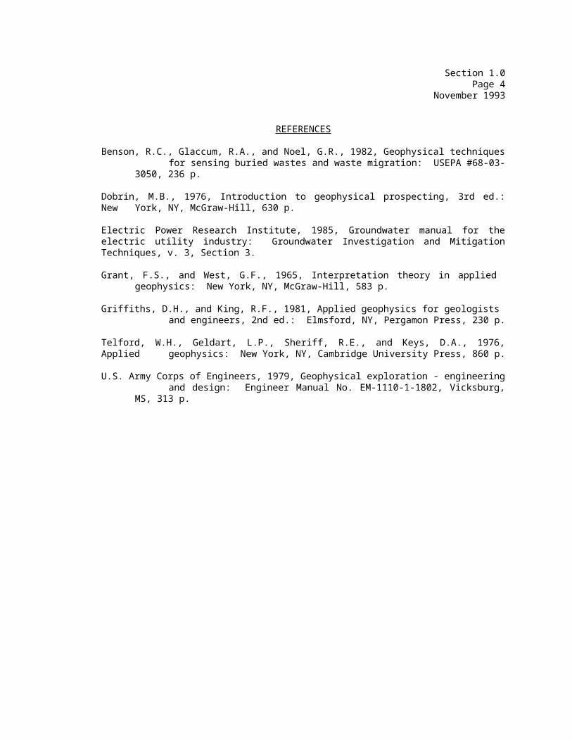
REFERENCES
Benson, R.C., Glaccum, R.A., and Noel, G.R., 1982, Geophysical techniques for sensing buried wastes and waste migration: USEPA #68-03-
3050, 236 p.
Dobrin, M.B., 1976, Introduction to geophysical prospecting, 3rd ed.: New York, NY, McGraw-Hill, 630 p.
Electric Power Research Institute, 1985, Groundwater manual for the electric utility industry: Groundwater Investigation and Mitigation Techniques, v. 3, Section 3.
Grant, F.S., and West, G.F., 1965, Interpretation theory in applied geophysics: New York, NY, McGraw-Hill, 583 p.
Griffiths, D.H., and King, R.F., 1981, Applied geophysics for geologists and engineers, 2nd ed.: Elmsford, NY, Pergamon Press, 230 p.
Telford, W.H., Geldart, L.P., Sheriff, R.E., and Keys, D.A., 1976, Applied geophysics: New York, NY, Cambridge University Press, 860 p.
U.S. Army Corps of Engineers, 1979, Geophysical exploration - engineering and design: Engineer Manual No. EM-1110-1-1802, Vicksburg,
MS, 313 p.
COMMONWEALTH OF MASSACHUSETTS
DEPARTMENT OF ENVIRONMENTAL PROTECTION
STANDARD REFERENCES FOR GEOPHYSICAL INVESTIGATIONS
SECTION 2.0 PLANNING A GEOPHYSICAL INVESTIGATION
Section 2.0Page i
November 1993
SECTION 2.0PLANNING A GEOPHYSICAL INVESTIGATION
TABLE OF CONTENTS
Section Title Page No.
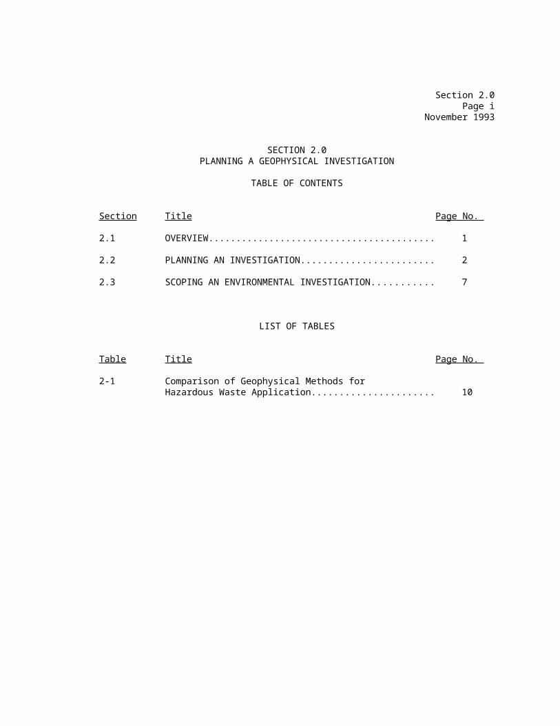
2.1 OVERVIEW......................................... 1
2.2 PLANNING AN INVESTIGATION........................ 2
2.3 SCOPING AN ENVIRONMENTAL INVESTIGATION........... 7
LIST OF TABLES
Table Title Page No.
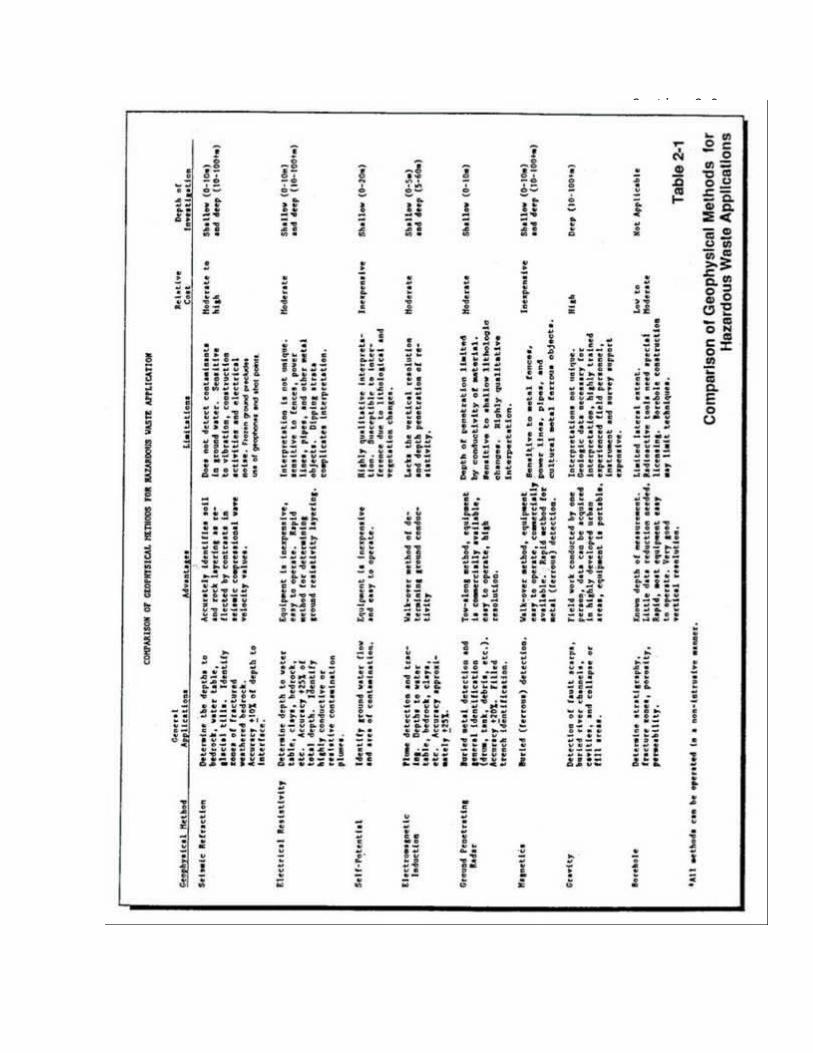
2-1 Comparison of Geophysical Methods for Hazardous Waste Application...................... 10
Section 2.0Page 1
November 1993
2.0 PLANNING A GEOPHYSICAL INVESTIGATION
2-1 OVERVIEW
Most of the environmental investigations conducted in the State of Massachusetts are regulated by one or more of a comprehensive set of Codified Massachusetts Regulations (i.e., 310 CMR 40.0000, known as the Massachusetts Contingency Plan). These regulations prescribe a comprehensive set of data collection criteria which includes the investigation of physical site characteristics, as well as the identification of source and the nature and extent of contaminants released to the environment.
The physical characteristics of a site which geophysics can help determine include: characterization of the types of overburden materials and thickness, as well as soil classification and permeability; characterization of the types of bedrock and depth to bedrock; characterization of water table elevations, hydraulic gradients, groundwater flow direction; and identification and characterization of all other physical site characteristics such as buried utility lines, sewers, and water mains.
In certain instances, geophysics can also be used to help identify the source and extent of release of contaminants by helping to establish: the source(s) of all releases of oil or hazardous material; the horizontal and vertical extent and (relative) concentrations of oil or hazardous materials in some media; the estimated volume of contaminated soil and (ground) water; all existing and potential pathways, including potential soil and groundwater pathways; and the existence of plume(s) of oil or hazardous materials in the groundwater and the potential migration of the plume.
Given the many potential uses of geophysics, as listed above, one might conclude that geophysics should be used on all investigations. This is not the case. All of the site characterization and source determination tasks listed above can be accomplished, often more accurately, by means other than geophysics. The question that must be asked in planning any environmental investigation is: What are the most cost effective methodologies to collect and analyze the data needed to achieve the project goals?
If data can be collected most cost effectively by a conventional means such as test pitting, then test pitting should be employed. If, on the other hand, it is determined that a geophysical method is quicker and more cost effective to collect data then the geophysical method should be employed. The key to this decision making process is an understanding of the following: 1) site history; 2) the scope and objectives of the investigation; 3) known or anticipated geologic conditions; 4) general
Section 2.0Page 2
November 1993
site conditions; and 5) the operating principles, applications, strengths, and limitations of the various geophysical methods outlined in this document.
The first four areas of required information must be collected and used in order to design any field investigation program. Knowledge in the fifth area (geophysics) will increase the chances that the investigation will be performed in the most cost effective manner possible. Striving for optimum cost effectiveness is critical for two important reasons. Increasing cost effectiveness benefits the client, since any decrease in amount which must be spent to evaluate and remediate a problem can be spent in other vital areas for corporate survival, such as R&D or sales. Maximum cost effectiveness benefits the project manager's company because it allows them to be more effective competitors in an increasingly price conscious market.
No attempt will be made in this section to cover the infinite number of possible combinations of project goals, geologic conditions, and site conditions that could present themselves to a project manager. No attempt will be made to outline the infinite number of applications that the various geophysical techniques could have to the project scenarios alluded to above. This section will instead attempt to provide a conceptual guide to the decision making process which must be employed when deciding upon the applicability of the various geophysical techniques to the specific problem at hand.
2.2 PLANNING AN INVESTIGATION
There are no simple formulas or guidelines which can be applied to make the determination as to whether geophysics should be used. The decision regarding whether or not to employ geophysics is job specific.
In order to plan an environmental field investigation, including the decision regarding the use of geophysics, a project manager must take the following factors into consideration:
o Site history
o The scope and objectives of the investigation
o Known or anticipated geologic conditions
o General site conditions
o Operating principles, applications, strengths, and limitations of geophysical techniques
The historical usage of a site (and the areas surrounding a site) and the environmental incidents which occurred on or in the vicinity of a site are the primary factors which are responsible for the site's current environmental condition. An understanding of these historical factors,
Section 2.0Page 3
November 1993
therefore, plays a vital role (along with time and money constraints) in determining the objectives and scope of an environmental investigation. The objectives and scope will, in turn, dictate the applicability of geophysical methods.
Both the objectives and the scope of an environmental investigation is the first determinant in the decision regarding the use of geophysics and the type of method(s) to be used. For example, if an objective is to define the overburden geology in an area known to have shallow bedrock and the area of investigation is a one quarter acre site, then conventional soil borings program would probably be a less expensive and more direct method of achieving the project goal than a seismic refraction survey. If, on the other hand, the objective is to define overburden geology at a 200 acre site where the depth to bedrock is unknown, then a combination of seismic refraction, to delineate the subsurface stratigraphy (because of it's speed and ease of data collection over large areas), combined with a limited soil boring program (for physical correlation and confirmation of stratigraphic interpretations) is probably a more effective approach. Geologic conditions of a study area, both known and inferred, will also play an important role in the decision regarding the use of geophysics and the type of method(s) to be used. As an example, Ground Penetrating Radar (GPR - Section 7.0) can be an effective tool in delineating conductive contaminant plumes. The depth of investigation for GPR, however, is extremely reduced by the presence of saturated clay layers. If shallow clay is known to be present, then GPR is not the geophysical technique of choice for conductive contaminant plume delineation; using electromagnetic induction methods would be a better choice.
Site conditions often have a considerable impact on the ability of a geophysical technique to collect the needed data. A site walkover should be conducted before planning any field investigation. The presence and location of: metal objects and/or fences; overhead power lines; paved and unpaved areas; traffic conditions; vegetative cover; marsh or swamp areas; and other site conditions must be noted and applied to the decision making process regarding the investigative mix to be employed at the site. As an example, if a stated project objective is to determine the presence and orientation of bedrock fractures. A Very Long Frequency (VLF - Section 6.0) study is an excellent method for doing this and can be performed on the surface, however, it is extremely sensitive to interferences from metal fences (long, linear conductors). The site walkover reveals that the area is extremely developed and that metal fences criss-cross the study area. Instead of VLF, this investigation will probably require rock coring and a borehole geophysical method (Section 10.0).
Knowledge of the operating principles, applicability, strengths, and limitations of the various geophysical methods is vital to a project planning process contemplating the use of geophysics. As can be seen in
Section 2.0Page 4
November 1993
the above examples, the correct decision regarding the applicability of a geophysical method(s) cannot be made without such an understanding. This decision must be made in context of the total project, including the objectives, scope, and site conditions (both surface and subsurface). Geophysical methods should be chosen based upon their applicability to fulfilling a specific data requirement and for their insensitivity to site specific conditions (e.g., metal fences) which could interfere with data collection. For example, a terrain conductivity survey (Section 6.0) is an excellent method for quickly surveying an area for changes in subsurface conductivity (which could be due to buried metal, conductive contaminant plumes, etc.). Terrain conductivity instrumentation, however, is extremely susceptible to interferences from overhead power lines and metal fences. If during site reconnaissance, you identified these interferences and you felt that a subsurface survey was required, then a conventional resistivity survey (Section 4.0) would be more applicable. Table 2-1 presents a synopsis of the most commonly used geophysical methods and the applications, advantages, and limitations of each.
Each method is described in detail in the following sections of this document. The reader is encouraged to begin the learning process by reading the overview of a geophysical method(s), which is presented at the beginning of each of the following sections. Should the particular method appear to be promising (with respect to the particular data collection requirement at hand), the reader should read the entire application section to gain a more complete understanding of the method being evaluated for use.
The following are two hypothetical cases which are provided as conceptual decision making guides.
a) Gas Station Scenario
The background for the first case is as follows: a gas station which reportedly has a leaking underground storage tank. The site is a one quarter acre property and the property owner has accurate "as built" diagrams and photographs of the installation. A check of the existing literature reveals that the USGS has published overburden and bedrock maps for the area. A review of the existing literature reveals that the subsurface consists of approximately 100 feet of medium sand overlying igneous bedrock. A review of the surrounding topography infers a direction of groundwater flow, which is confirmed by review of another environmental study of a nearby gas station. This site is not a good candidate for geophysics. The suspected source area is known, the subsurface geology is well defined, the direction of groundwater flow has been determined before the start of drilling and the contaminant of concern is relatively insoluble and is lighter than water. The most cost effective course of action at this stage would simply be to install and sample three (one upgradient and two downgradient)
Section 2.0Page 5
November 1993
water table wells to determine if a problem exists.
b) Landfill Investigation Scenario
The second case involves the investigation of an inactive, uncontrolled landfill which is approximately 100 acres in size, the actual boundaries of which are unknown. Nearby private water supply wells downgradient of the landfill have become contaminated with what appears to be leachate. In addition, a public bedrock supply well, which is screened at the base of the overburden and is side gradient to the landfill (with respect to regional groundwater flow), has become contaminated with high concentrations of chlorinated solvents.
The project goals are to: identify whether the landfill is the source of the different types of water supply contamination; and determine if the landfill contains the buried drums, which are reportedly the cause of the chlorinated solvent contamination and, if present, determine their location. This site would be a good candidate for the use of geophysics. Possible methods suggested for this investigation would be seismic refraction (Section 3.0), magnetometer (Section 8.0), terrain conductivity (Section 6.0), and resistivity (Section 4.0).
Seismic refraction could be employed to help determine the horizontal and vertical extent of the landfill and to map bedrock topography. The boundary between the disturbed landfill material and the undisturbed materials surrounding it would be readily apparent using a seismic refraction survey. The presence of high concentrations of chlorinated solvents at the base of the aquifer suggests that these solvents might be present as DNAPLs. The flow of DNAPLs would be controlled by bedrock topography. Seismic refraction can usually provide a much more detailed profile of the bedrock surface for far less money than would be possible with a conventional boring program.
As stated earlier, the landfill is 100 acres in size. One could simply hire a backhoe operator and start digging at one end of the landfill with the intention of continuing until the drums are found. Faced with this prospect, one would naturally hope that an easier solution would be available. Fortunately, such a solution does exist. A magnetometer survey of the entire landfill could be conducted in a matter of days and would locate ferrous metal anomalies, one of which could represent the suspected drums you are looking for. Instead of indiscriminate digging over a large area, one could concentrate specifically on the anomalies of concern. The result will be a considerable savings in time and money spent on this investigation.
Terrain conductivity could be used more precisely determine the
Section 2.0Page 6
November 1993
horizontal extent of the landfill and to locate and map a shallow leachate plume (usually highly conductive) emanating from the landfill. However, it should be noted that a chlorinated solvent plume, which is essentially nonconductive, would be invisible to the terrain conductivity instrument. The conventional investigative approach would be to place wells at regularly spaced intervals along the downgradient side of the landfill to try to locate the leachate plume(s). If the downgradient side of the landfill were 2,000 feet long, as many as 20 wells, spaced 100 feet apart, would be required to provide a sufficient level of coverage (and confidence) to characterize groundwater conditions. Terrain conductivity could be used to survey the entire downgradient side of the landfill in one day. The results of this survey would be used as a well installation guide and could easily reduce the number of wells required to characterize the water quality downgradient of the landfill by 75% and may be able to more accurately define the leachate plume location.
The decision to employ a conventional resistivity survey, either as a supplement to, or replacement of the terrain conductivity survey at this site would need to be based upon the availablity of pertinent site specific information. For example, if it is known that the depth to groundwater beneath the study area is greater than 30 feet, then the terrain conductivity device, which is limited in its depth of investigation, may fail to locate and delineate an existing leachate plume. Even if the water table is shallow, if the saturated overburden in the landfill area is extremely thick, then a sinking leachate plume emanating from beneath a portion of a landfill may pass beneath the study area at a depth that cannot be detected by the shallower operating terrain conductivity devices. In these specific instances, the resistivity survey, which has the greater depth of investigation, would probably be a better choice.
Given the possibility of the above examples, in the absence of such detailed subsurface data, it would appear that a prudent project manager would always specify that conventional resistivity be run as a precautionary measure. More often that not, however, it is not performed. The overiding reason for this (which is explored more fully in Section 4.0 of this document) is the expense involved in performing the conventional resistivity survey. The project manager who is almost always working under time and money constraints, usually cannot and probably should not, without compelling evidence demonstrating the need, initially specify such a time-consuming and expensive investigative technique. As the project progresses, data collected (it has been assumed that an intrusive investigative program will be instituted and will supplement geophysical data) may demonstrate the need for the additional, iterative level of effort and expense that the conventional resistivity survey represents. This possible outcome
Section 2.0Page 7
November 1993
is always present when attempting to design the most cost effective environmental investigation. In any environmental investigation, the project manager must constantly weigh the benefits of additional data collection against the ever present real world limitations of time and money constraints. Very often, data collection comprises must be made. It is one of the jobs of the project manager to decide where "the most bang for the buck" can be had when designing an environmental investigation program.
2.3 SCOPING AN ENVIRONMENTAL INVESTIGATION
Ideally, one would be able to consult a geophysicist before planning each field investigation to determine if the use of such procedures is warranted. If this document is utilized as intended, the reader will develop a general knowledge of geophysical applications, however, still will not be an expert. Whenever possible, the reader should work with a geophysicist to help develop the best mix of investigative techniques for the project.
Unfortunately, project time and money constraints will often preclude this luxury. It is, therefore, important that a project manager have a good working knowledge of the applications, strengths, and limitations of each technique in order to decide for themselves whether or not geophysics should be used. If it is necessary for a project manager to decide upon and specify a geophysical program to be used for the purpose of bid solicitation without the benefit of consultation, then the following recommendations are made:
1) Provide as much pertinent data concerning site conditions as possible.
As has been briefly touched upon in the above discussion and is covered in greater detail in the following sections, the applicability of, or approach to using, a geophysical method is often dictated by the site conditions. Since each method is sensitive to different conditions (which are outlined in each of the following sections, it is important to provide pertinent site data with the bid package.
2) Be specific in your data requirements as possible.
For example, do you simply need to know the location of underground storage tanks so that you can install downgradient wells or do you also need to know the orientation and width of the tanks in the ground because you wish to place soil borings adjacent to the tanks (to look for soil contamination) without drilling into them. Usually, the more specific your data requirements, the more expensive the
Section 2.0Page 8
November 1993
study. The natural inclination of most project managers inexperienced with geophysical techniques is to specify the absolute minimum coverage they may feel is necessary. It is better, however, to spend slightly more and get what you need than to spend slightly less and be dissatisfied with the results.
3) Be general in specifying your data collection methodologies.
Don't try to over-specify your bidding document. Tell the contractor the specific method to be employed, the specific data collection requirements and the specific area over which the data needs to be collected, but give them latitude in how best to collect your data (e.g., what geophone spacing to use over a study area).
4) Require a specific response to your bid package, but encourage submittal of alternate approaches (and their corresponding costs).
It is important that all bidding respondents be evaluated on an "apples to apples" basis. Your bid document should therefore require a specific response for evaluation purposes. One must not forget, however, that there is usually more than one approach to solving a problem and that the geophysical professional is the best qualified person to suggest a better one. Give the respondent the opportunity to be innovative and save you additional time and money, while achieving your project goals.
Section 2.0Page 9
November 1993
SECTION 2.0PLANNING A GEOPHYSICAL INVESTIGATION
LIST OF TABLES
Table Title Page No.
2-1 Comparison of Geophysical Methods forHazardous Waste Applications.................... 10

Section 2.0Page 10
November 1993
COMMONWEALTH OF MASSACHUSETTS
DEPARTMENT OF ENVIRONMENTAL PROTECTION
STANDARD REFERENCES FOR GEOPHYSICAL INVESTIGATIONS
SECTION 3.0 SEISMIC METHODS
Section 3.0Page i
November 1993
SECTION 3.0SEISMIC METHODS
TABLE OF CONTENTS
Section Title Page No.
3.1 OVERVIEW......................................... 1
3.2 INTRODUCTION..................................... 2
3.2-1 Seismic Reflection............................... 43.2-2 Seismic Refraction............................... 5
3.3 APPLICATIONS..................................... 5
3.3-1 Seismic Refraction............................... 53.3-1.1 Seismic Velocity Values and Layering............. 63.3-2 Seismic Reflection............................... 7
3.4 EQUIPMENT - Seismic Refraction................... 7
3.5 FIELD PROCEDURES................................. 8
3.5-1 Data Acquisition - Seismic Refraction............ 83.5-2 Specific Consideration - Seismic
Refraction....................................... 103.5-3 Seismic Reflection Surveys....................... 10
3.6 INTERPRETATION................................... 11
3.6-1 Refraction Data Interpretation................... 113.6-1.1 Critical Distance Method......................... 123.6-1.2 Time Intercept Method............................ 123.6-2 Reflection Data Considerations................... 13
3.7 ADVANTAGES AND LIMITATIONS - REFRACTION AND REFLECTION................................... 13
3.7-1 Seismic Refraction............................... 143.7-2 Seismic Reflection............................... 15
3.8 GLOSSARY......................................... 15
REFERENCES ................................................. 17
SELECTED REFERENCES.......................................... 18
Section 3.0Page ii
November 1993
SECTION 3.0SEISMIC METHODS
TABLE OF CONTENTS (continued)
LIST OF FIGURES
Figure Title Page No.
3-1 Seismic Wave Paths for Direct Wave, Reflected Wave, and Refracted Wave Illustrating..................................... 23
(a)......Effects of a Boundary Between Materials with Different Elastic Properties........... 23
(b) Snell's Law................................. 23
3-2 Field Layout of a Multi-Channel Seismograph Showing the Path of Direct and Refracted Seismic Waves in a Two-Layer Soil/Rock System........................................... 24
3-3 Guide to Material Identification by P-Wave Seismic Velocity................................. 25
3-4 Example of Seismic Refraction Analog Record.......................................... 26
3-5 Critical Distance Technique of Data Interpretation................................... 27
(a) Travel-time Plot........................... 27
(b) Interpreted Profile......................... 27
3-6 Flow Diagram Showing Steps in Processing and Interpretation of Seismic Refraction Data ............................................ 28
3-7 Time Intercept Technique of Seismic Data Interpretation................................... 29
(a) Travel-time Plot............................ 29
(b) Interpreted Profile......................... 29
Section 3.0Page iii
November 1993
SECTION 3.0SEISMIC METHODS
TABLE OF CONTENTS (continued)
LIST OF FIGURES
Figure Title Page No.
3-8 Solution of Seismic Refraction Data.............. 30
(a) Travel-time Plots of First Arrivals Along a 400-ft. Seismic Geophone Spread...................................... 30
(b) Resulting Profile of Subsurface Materials Showing Interface Between Different Velocity Layers........... 30
Section 3.0Page 1
November 1993
3.0 SEISMIC METHODS
3.1 OVERVIEW
The seismic methods of geophysical exploration are active (manmade energy sources are used) techniques used to characterize subsurface geology. These methods are an indirect means of determining the type and thicknesses of the various materials underlying a site. The general principle of seismic surveying is that dissimilar subsurface materials can be determined by the differences in their respective physical properties. Each material has a unique set of physical properties (elastic moduli, density, and Poisson's ratio) which effect the amplitude and velocity of seismic waves traveling through them. Seismic surveys are conducted by inducing seismic energy into the subsurface and measuring the resultant velocity and amplitude of the seismic waves by detectors located on the ground surface. The resultant data can be used to infer the types of material present in the subsurface.
There are two basic methods of seismic surveying: reflection and refraction. The basic methodology for these seismic techniques consists of actively generating waves in the ground and detecting them at ground surface after they have either reflected or refracted off of subsurface layers. The energy (seismic waves) is generated by various means such as weight drops, explosives, mechanical sources, etc. Electromechanical transducers (which turn ground motion into electricity), called geophones, are used to detect the arrival time and amplitude of the induced ground motion. The instrumentation system is referred to as the seismograph. Arrays of geophones, called seismic spreads, are connected by electrically conductive cables to the seismograph, which processes and records the collected data. Recordings are made with either analog or digital seismographs. Preliminary data evaluation can usually be performed in the field with analog recordings. Playbacks of digital recordings are performed in the office for final data processing and report preparations.
The seismic reflection method involves the introduction of energy to the ground and the measurement of sound waves which are reflected (bounced back) from the subsurface interfaces of material types. These interfaces can be either the contact of different geologic strata or the boundary of the saturated and unsaturated zone within the same geologic strata.
A seismic refraction survey involves the measurement of those sound waves which move down through overlying material and refract (move along) along the subsurface material interface and eventually propagate back to the ground surface. For reasons that will be described in the introduction, seismic refraction is by far the most prevalent method used in the shallow subsurface studies (less than 300 feet) employed during environmental investigations in Massachusetts and New England. This section will therefore focus, as a matter of practicality, on the seismic
Section 3.0Page 2
November 1993
refraction method.
Seismic refraction surveys can be employed to: delineate the types and thicknesses of geologic materials; determine depth to groundwater; correlate stratigraphy across a study area (in conjunction with test pit and/or boring log data); detect sinkholes and cavities; detect bedrock fracture zones; determine extent of landfills; and determine extent of filled areas such as reclaimed quarries. When a seismic refraction survey is performed prior to an intrusive field investigation, the data can be used to help determine the number, distribution, and depth of test pits, borings, and monitoring wells. When a seismic refraction survey is performed after intrusive field investigation, the use of physical data to calibrate refraction data allows the interpolation of subsurface conditions across large areas with a great degree of confidence. Intrusive field data can also be used to refine the interpretations of seismic data which had been collected prior to the start of the intrusive field program.
Seismic refraction does have limitations. The first is cost. Seismic refraction surveys cost between $2,000 and $4,000 per day. For smaller investigations, which might only require the installation of a few soil borings and water table monitoring wells, it probably would not prove cost effective to employ seismic refraction. Seismic refraction surveys by nature are sensitive to ground vibrations. Unfortunately, many human activities, including vehicle traffic, construction, and manufacturing, can create noise (unwanted ground vibrations) which can make collection of wanted data in a particular area difficult if not impossible. Seismic refraction surveying is seasonal. Frozen ground conditions make data collection difficult if not impossible. Interpretation of seismic refraction data is often non-unique. Some measured velocity values readily correlate with specific geologic materials such as massive, intact bedrock. Other velocity values, however, do not correspond to a unique interpretation of the nature of the materials surveyed and require correlation with soil borings or test pits for exact determination of the conditions and types of geologic layering.
For larger investigations, however, especially those that require the delineation of bedrock competence and topography (DNAPL investigations), the combined use of seismic refraction with conventional investigative techniques can often result in a higher level of data volume and quality, while providing a considerable savings of time and money for the project.
3.2 INTRODUCTION
When an artificially generated energy pulse (e.g., small explosion) is applied to the earth, waves migrate from the source through the earth just as waves move away from a stone dropped in water. There are four types of seismic waves generated by a near-surface seismic energy source: Love Waves, Rayleigh Waves, Compression (P) Waves, and Shear (S) Waves. Love waves and Rayleigh waves are confined to the near surface, while
Section 3.0Page 3
November 1993
compressional (P) and Shear (S) waves can travel both along the surface and through the body of the earth. The two types of seismic waves used in seismic exploration are the compressional (P) wave and the shear (S) wave. Particle motion resulting from a P-wave is an oscillation, consisting of alternating compressions and dilatations (a push-pull motion), in the direction of propagation. An S-wave causes particle motion transverse (perpendicular) to the direction of propagation. The P-wave travels with the higher velocity of the two waves, represents the first arrival of refracted waves at the geophone (detector) located on the ground surface, and is therefore of greater importance for seismic surveying. The following discussions are concerned principally with P-waves.
There are four possible paths for wave energy to take as it moves through the earth. The energy can: 1) move directly from the energy source to the surface detector (direct wave); 2) travel down through the earth until it encounters a material interface and is totally reflected back up to the surface; 3) travel down to encounter a material interface and be partially reflected up, while the remainder of the energy is refracted (deflected) to travel along the interface boundary; or 4) travel down to encounter a material interface and be partially reflected up, while the remainder of the energy is refracted but continues to travel deeper into the earth. It should be noted that the energy which continues to move deeper (as described in possibility #4 above) will encounter other material interfaces at which point possibilities 2, 3, or 4 as described above would again apply. The different possibilities of wave propagation are illustrated in Figure 3-1a.
The path that the wave energy will take as it encounters material interfaces is dependent upon the angle at which the wave strikes the interface (angle of incidence), as well as the density and acoustic velocity (the velocity that sound can travel through a given material) contrast of the two materials. When a wave traveling through a media encounters a layer of higher velocity, the wave is refracted (deflected) towards the horizontal. This phenomena is similar to the refraction of light as it passes into water which manifests itself as the apparent bend (towards the horizontal) of the submerged portion of a vertical stick. Since, as a general rule, the earth exhibits greater densities and higher acoustic velocities with depth, eventually most of the energy (which has not been attenuated by the earth materials) introduced at the surface will return to the surface.
The "critical angle" is the angle of incidence which, for a given material velocity contrast, will cause the energy wave to refract horizontally (i.e., Figure 3-1b where _2 = 90) and travel along the material boundary interface. As the acoustic energy travels along the material interface it creates disturbances in the lower portion of the upper zone at each point that the wave passes. These disturbances in turn act as energy sources which create seismic waves. These same waves are then refracted back to the surface where they are detected by the

Section 3.0Page 4
November 1993
geophone spread. The "critically" refracted wave travels from energy source to geophone (receiver) in the shortest possible amount of time. The travel path and travel time of the refracted waves are functions of the properties and geometry of the subsurface, and can be analyzed to produce a vertical profile of the subsurface. Information such as the number, thickness and depths of stratigraphic layers, as well as indicators as to the composition of these units, can often be ascertained.
The first wave arrivals at the geophones located very near the energy source are the direct waves that travel through the near-surface materials. At greater distances, the first arrival is a refracted wave as illustrated in Figure 3-2. Lower layers typically are higher velocity materials; therefore, the refracted wave will overtake both the direct wave and the reflected wave, because the time gained traveling through the higher velocity material compensates for the longer wave path. Depth computations are based on the ratio of layer velocities and the distance from the energy source to the point where refracted wave arrivals overtake direct arrivals.
More rigorous discussions of seismic wave theory as applied to seismic reflection and refraction can be found in Dobrin (1976), Telford and others (1976), Griffiths and King (1981), and Mooney (1977).
3.2-1 Seismic Reflection
The basis for seismic reflection surveying is the time required for a seismic wave to travel from the source to a discrete reflector interface, and for the reflected wave to return to the surface (two-way travel time). Both the energy of the reflected wave and the diagnostic wave form are a function of the acoustic impedance contrast across the subsurface material interface. Acoustic impedance characteristics of a material depend on its seismic velocity and density.
Seismic reflection surveys are superior to refraction surveys in that they do not require that each successive material layer has a velocity greater than the one above it. The reflection method also provides greater resolution and accuracy, use smaller charges, uses shorter geophone spreads, and can measure larger numbers of material interface horizons.
Seismic reflection surveys predominate in the petroleum exploration business, while seismic refraction surveys have comprised the majority of environmental surveys. Seismic reflection surveys are generally used on land for deeper depths of investigation (hundreds of feet). High resolution shallow reflection surveys have had some limited success in the upper few hundred feet, but only under ideal conditions (flat surface topography and subsurface layering). For underwater operations in bays and harbors, the reflection method is often useful; as a rapid and effective technique to profile sub-bottom layering, it is usually
Section 3.0Page 5
November 1993
complemented by refraction measurements. It is important to note that the reflection technique does not directly measure seismic velocities, a necessary element to interpreting subsurface seismic data from a hydrogeologic viewpoint.
3.2-2 Seismic Refraction
Despite the advantages of seismic reflection (which are discussed in the previous subsection), seismic refraction remains the method of choice for environmental studies in New England. The most overriding reason for this situation is cost. The sophisticated equipment (and expense) required for a reflection study are not normally required to meet the data collection requirements of an environmental study. Refraction surveys can collect required data much more cost effectively. In addition, the refraction method is superior in characterizing the shallow alluvial and glacial overburden or areas with uneven topography and/or steeply dipping bed boundaries which are often found in New England.
Unlike reflection, refraction does not require any prior knowledge of subsurface material acoustic velocities to interpret data. This is very important given the often exploratory nature of environmental studies.
3.3 APPLICATIONS
For projects where a rapid and non-invasive method of profiling subsurface conditions is desired, the seismic methods (the refraction technique, in particular) have widespread use and acceptance. The extent of use and the anticipated results will depend on site specific conditions related to the geologic setting and the desired objectives.
3.3-1 Seismic Refraction
The seismic refraction technique is a particularly accurate and effective method for determining the thicknesses of subsurface geologic layers. Applications for groundwater and hydrogeologic studies include:
o Continuous profiling of subsurface layers including the bedrock surface;
o Determinations of water table depth;
o Mapping and general identification of significant stratigraphic layers;
o Detection of sinkholes and cavities;
o Detection of bedrock fracture zones; and
o Detection of filled-in areas (e.g., reclaimed quarries).
Section 3.0Page 6
November 1993
Seismic refraction investigations are especially significant because the measured seismic velocities can be used for geologic material identifications. Figure 3-3 presents a guide to material identification based on P-wave seismic velocity values.
3.3-1.1 Seismic Velocity Values and Layering
Seismic compressional wave velocities in unconsolidated deposits are significantly affected by water saturation. The seismic velocity values of unsaturated overburden materials such as gravels, sands and silts generally fall in the range of 1,000 to 2,500 ft/sec. When these materials are water saturated, that is when the space between individual grains is 100% filled with water, the seismic velocities range from 4,800 to 5,100 ft/sec., nearly equivalent to the compressional P-wave velocity of sound in water. A small decrease in the saturation level will substantially lower the measured P-wave velocity of the material. Because of the large velocity contrast between saturated and unsaturated materials, the water table acts as a readily identifiable refractor. Glacial tills often exhibit an acoustic velocity in the range of 6,000 to 8,000 ft/sec. Bedrock in Massachusetts includes igneous, metamorphic, and sedimentary deposits. There are a wide range of acoustic velocities associated with these formations, but in almost all cases these velocities are higher than those of the overburden materials and can be detected with the refraction technique.
Seismic investigations over unconsolidated deposits are used to map stratigraphic discontinuities and to determine the stratigraphy of the subsurface. These discontinuities can be horizontal (a dense till layer beneath a layer of saturated sands and gravels) or vertical (the lateral boundaries of a landfill or other manmade fill material). Often these boundaries represent significant hydrologic boundaries, such as those between aquifers and aquicludes.
A common use of seismic refraction is the determination of the thickness of a water saturated layer in unconsolidated sediments and the depth to relatively impermeable bedrock or dense glacial till. Continuous subsurface profiles and even contour maps on the top of a particular horizon or layer of interest can be developed from a suite of seismic refraction data.
Bedrock velocities (Figure 3-3) vary over a broad range depending on variables which include:
o Rock type
o Density
Section 3.0Page 7
November 1993
o Degree of jointing/fracturing (and fracture saturation for compressional waves)
o Degree of weathering
Fracturing and weathering reduce seismic velocity values in bedrock. Low velocity zones of seismic data should be evaluated to determine if they are due to conditions in overburden or in bedrock (e.g., fractures, weathering, and faulting).
3.3-2 Seismic Reflection
Seismic reflection surveys are generally used on land for the deeper depths of investigation (thousands of feet) required in petroleum exploration. The reflection method is often useful as a rapid and effective technique for profiling sub-bottom layering in bays and harbors, it is usually complemented by refraction measurements.
3.4 EQUIPMENT - Seismic Refraction
The basic equipment necessary to conduct a seismic refraction investigation consists of:
o Seismometers (geophones) and cables
o Seismograph
o Energy source
Geophones are electromechanical transducers which convert ground motion into an electric voltage which is used to record the seismic wave arrivals. Seismic cables link the geophones and amplifier, and are fabricated with pre-measured locations for geophones. The voltage output can be amplified and filtered for individual geophone.
Recording of seismic data is conducted in either analog or digital format with single or multi-channel recording equipment usually referred to as the seismograph. Multi-channel data acquisition systems (12- or 24-channel) are much preferred and necessary for all but the simplest of very shallow surveys. In general, a greater number of channels results in higher resolution of seismic velocities and depth determinations. Analog records are paper prints of the geophone response to seismic wave arrivals. The travel time between the shot and the arrival of the seismic wave can be measured directly for each geophone. Figure 3-4 is an example of an analog record showing one horizontal trace for each geophone, vertical timing lines, zero-time break, and the first arrival signals at each geophone. Seismic data recorded digitally readily permit subsequent computer processing and more extensive and detailed interpretation of seismic data.
Section 3.0Page 8
November 1993
Energy sources used for seismic surveys are categorized as either non-explosive or explosive. The energy for a non-explosive seismic signal can be provided by one of the following:
o Airgun (usually marine surveys)
o Seisguns
o Weight drop
o Sparker (marine surveys)
o Sledge hammer (shallow penetration)
o Vibrators (for reflection surveys)
Explosive sources can be categorized as:
o Dynamite
o Primers
o Blasting agents
The choice of the energy source is dependent on site conditions, depth of investigation, and seismic technique chosen as well as possible local restrictions. Explosive sources may be prohibited in certain areas (such as urban areas) where non-explosive sources can be routinely used. Deeper investigations usually require a larger energy source; therefore, explosives may be required for sufficient penetration. It should be noted that explosives provide the best data, but a qualified blaster is required.
3.5 FIELD PROCEDURES
Since seismic surveys in Massachusetts locales are almost always conducted using the refraction technique. The following discussions are principally concerned with refraction, and highlight specific aspects of interest for monitoring well installations.
3.5-1 Data Acquisition - Seismic Refraction
Seismic refraction surveys may be conducted on a grid basis, or along a single line (with perpendicular cross-check lines) depending on the survey objectives, site size, and time and budget constraints. Obtaining data on a grid allows a three-dimensional subsurface stratigraphic map to be produced. Additional seismic energy source points located along the profile will produce more seismic data with which to construct subsurface profiles. Additional survey techniques for assessing lateral variations include broadside shooting, in which the shotpoints and geophones are
Section 3.0Page 9
November 1993
located along parallel lines, and fan shooting, in which the geophones are laid out in a fan shape with the shot point at its apex.
Seismic spread cables, which have been fabricated with pre-measured shotpoint and geophone locations, are positioned along the lines of investigation. Geophones, fitted with a spiked base to provide "coupled" ground contact, are positioned at their measured locations. To acquire seismic refraction data, a specific number of geophones are spaced at regular intervals along a straight line on the ground surface; this line is commonly referred to as a "seismic spread". The length of spread determines the depth of penetration; a longer spread is required for a greater depth of penetration. Spread length should be approximately three to five times the required depth of penetration. Required resolution of velocity values and interface irregularities will control the number of geophones in each spread and the distance between each geophone. Closer spacings and more geophones usually result in more detail and greater resolution.
The locations of individual seismic spreads and profile lines should be consistent with the desired subsurface information. Where a bedrock depression feature is suspected, seismic lines should be oriented perpendicular to the suspected trend of the feature. Seismic cross profiles may be necessary to confirm depths to a particular refracting horizon, especially when there are steeply dipping layers involved as on the edge of the bedrock valley. At a site where little information is known about subsurface layering trends, at least two seismic lines oriented in a "T" or "L" arrangement should be completed and the data assessed before further refraction profiling takes place.
The topography of a site dictates whether or not surveyed elevations are required. If possible, refraction profile lines should be positioned along level topography. For highly variable topography, a continuous elevation profile may be required to ensure sufficiently accurate cross-sections and to permit the use of time corrections in the interpretation of the refraction data. Knowledge of site geology can be helpful when planning the seismic energy source. Some geologic materials, such as loose, unsaturated alluvium and peat deposits, do not transmit seismic energy well and a larger seismic energy source may be required. Geologic conditions also dictate whether or not drilled shotholes are required.
Seismic energy is generated with either a weight impact (sledge hammer) or small buried charges of explosives. If explosives are used, shotholes are usually prepared with a driven rod (not excavated) to insure maximum energy transmission after the shothole has been made. Explosives are inserted, tamped and the depths and amount of explosives used are noted.
Seismograms are typically obtained using a portable signal enhancement seismograph which records the wave arrivals from the energy source along the seismic spread, acquiring separate data for each geophone position. Timing lines are provided across the entire recording allowing direct
Section 3.0Page 10
November 1993
reading of wave arrivals to an accuracy of one millisecond. The signal enhancement capability refers to the ability of the instrument to record the seismic waves from several impacts (or explosions), add them electronically, and retain this data in its internal digital memory for later processing and interpretation. The enhanced signal improves data quality and greatly facilitates interpretation.
Generally, several recordings are obtained along each seismic spread; seismograms are generated with the energy source at each end, and others may be obtained by energy generation in the middle, and at other positions along an individual seismic spread as necessary. The most commonly used method of seismic refraction surveying is reversed profiling. It is accomplished by setting out a straight-line array of geophones and then recording the signals caused by a source at one end and then reversing the procedure with source of energy at the other end, allowing the production of a two-dimensional subsurface cross-section. Continuous profiling is accomplished by having an end shotpoint of one seismic spread coincident with an end or intermediate position shot point of the succeeding spread. Field records must include the coordinates (or stations) of all receiver locations and shotpoints as well as specifics of the seismic energy source, electronic filtering and amplification used, and, in the case of direct read-out seismographs, the travel times in milliseconds.
3.5-2 Specific Considerations - Seismic Refraction
Since the seismic method measures ground vibration, it is inherently sensitive to noise from a variety of sources such as traffic and wind. Signal enhancement is a significant aid when working in noisy areas and with smaller energy sources. Enhancement capability is available in most single and multi-channel systems. Enhancement is accomplished by adding a number of seismic signals from a repeated source (e.g., multiple hammer blows). Noise, which is random by nature, will cancel itself out with repeated signal additions, while the actual seismic signal, which is not random, will be enhanced by repeated additions. This process can result in a more accurate measurement of the first arrival time, permits operation in noisier environments, and allows operation of at greater source-to-geophone spacings.
Cultural effects such as vibration-generating activities, on-site utilities and buildings often affect where data can be acquired and where the lines should be located. High volume traffic areas may require nighttime data acquisition. If the survey is to be conducted near a building where vibration-sensitive manufacturing is conducted, data acquisition may be constrained to particular time intervals and appropriate energy sources must be used.
3.5-3 Seismic Reflection Surveys
As noted earlier in this section, the seismic reflection technique has
Section 3.0Page 11
November 1993
not been used on any significant amount of environmental investigations in New England. Although it is acknowledged that some usefulness exists for professionals involved with other geologic locales, the present state-of-the-art experience warrants only a brief discussion in this document.
The field procedures for reflection are similar to refraction, requiring the use of geophones, multi-conductor cables and an energy source. The geophone spacings and lengths of cables are generally much shorter for reflection than for refraction for shallow penetration studies (a few hundred feet or less below the earth's surface). The energy source would be smaller than refraction requires. Data recordings, however, must be made with appropriate digital equipment to accommodate the larger amount of data "samples".
Before reflection data can be interpreted, an intensive effort of data processing is required. This processing is much more intensive (and expensive) than processing of refraction data requires. The final product of data processing is usually variable density type of plot with waveforms that reflectors such as the subsurface boundaries/layer of interest prior to drilling.
3.6 INTERPRETATION
The results of any seismic survey are usually presented in profile form showing elevations of stratigraphic horizons. The interpreter needs to be aware of travel time anomalies, lateral velocity changes and apparent velocities, and be capable of calculating "true" velocities and dip angles. The text book case of two or three horizontal stratigraphic layers is the exception rather than the rule in Massachusetts geology. Data acquired on a grid basis can be contoured and used to construct stratigraphic contour maps. Seismic velocities and the corresponding generalized material identifications should be presented on the subsurface profiles along with any test boring data used for correlation.
3.6-1 Refraction Data Interpretation
Interpretation of seismic refraction data involves solving a number of mathematical equations using the refraction data as it is presented on a travel-time versus distance plot. Analog seismic refraction data can be processed by hand plotting the data and using a hand calculator or by using a computer model to make the necessary calculations. Travel times for the first arrival waves at each geophone are measured from the analog record (see Figure 3-4). For a site containing horizontal stratigraphic layers of increasing velocity, the travel time chart (Figure 3-5) will consist of a series of overlapping straight line segments of decreasing slope. The inverse slope (1/v) of each line segment is equal to the seismic velocity in a layer. Using these velocities, the critical angle of refraction for each boundary can be calculated using Snell's Law. Then, utilizing these velocities and angles and the recorded distances to
Section 3.0Page 12
November 1993
crossover points (i.e., where line segments cross), the depths and thicknesses of each layer can be calculated using simple geometric relationships.
Thicknesses of velocity layers are calculated by either the critical distance or time intercept methods (Redpath, 1973). Accurate depth calculations are dependent on the assumption that the velocity of each geologic layer increases with depth. If that is not the case, additional corrections must be applied. Figure 3-6 is a diagram showing the steps in processing and interpreting seismic refraction data.
3.6-1.1 Critical Distance Method
A sample time-distance plot illustrating the critical distance method is shown on Figure 3-5. The critical distances, X12 and X23, are determined by constructing a line from the intersection of the two straight-line velocity segments perpendicular to the x-axis. Depths to refracting horizons are calculated using the critical distance and the layer velocities.
3.6-1.2 Time Intercept Method
The time intercept method is illustrated on Figure 3-7. Time intercept values for each layer are determined by extending the velocity line segments to intersect the y-axis. That intersection is the time intercept for that layer. Depths using the time intercept method are calculated from the intercept time and the layer velocities .
An interpreted profile section is illustrated on Figure 3-8. This section was produced using the critical distance method. If the profile had not been "reversed" (i.e., had there not been a shot at each end), the dipping interfaces and the stratigraphic detail would not have been evident. Important corrections which should also be evaluated are:
o Depth of shot
o Topography
o Velocity inversions
There are a number of possible complicating factors. While reverse profiling will reveal dipping boundaries, the calculation of dips, true depths and true velocities requires additional data processing. Furthermore, ground surface elevation corrections, as well as corrections to account for weathered bedrock zones must often be made before data can be correctly interpreted. Fracturing and weathering in bedrock generally reduce seismic velocity values. Consequently, travel-time plots with late arrivals must be evaluated carefully to determine if the late arrival times (slower velocities) are due to overburden conditions or fractured/weathered bedrock. The presence of undetected very thin layers
Section 3.0Page 13
November 1993
or low velocity zones can lessen the accuracy of interpretation.
Refraction theory is based on the assumption that material velocities increase with depth. If a velocity inversion exists (i.e., a low velocity layer is overlain by a higher velocity layer), depths and seismic velocities can be calculated but the uncertainty in calculations is increased unless borehole velocity data are available. Since irregular boundaries are not adequately resolved with time-distance analysis, another form of analysis involving delay-time is often used. The most complete interpretation of refraction data is often performed by computers using software to complete complex and numerous mathematics computations too time-consuming to be performed manually.
Although seismic refraction is very useful in confirming subsurface structures and performing reconnaissance surveys, it should be noted that multiple interpretations for each data set are possible. Additional independent information for correlation purposes such as borings, test pits and possibly other types of geophysical survey information are very important to insure the accuracy of the interpretation.
3.6-2 Reflection Data Considerations
Reflection surveys are usually conducted with shorter spreads but with more geophones compared to a comparable refraction survey. Given the increased number of data collection points, a significantly greater amount of data recording and data processing must therefore take place as an integral part of the interpretation process. In addition to the first arrival, numerous reflected arrivals are recorded at each geophone. Most seismic reflection data are recorded digitally, computer processed and then interpreted. Corrections that should be applied include, but are not limited to:
o Normal move-out (correction for source-to-geophone distances)
o Overburden thickness (the "weathering" correction)
o Migration of reflector points
o Signal filtering and enhancement
After computer processing, the data are printed in various types of displays, such as a variable density plot on which waveforms show discrete reflectors representing material boundaries. A cross-section based on horizontal distance versus travel time can be constructed from this plot. Only after a depth calibration is provided by means of drilling or velocities determined by uphole/ downhole or refraction surveys can a geologic cross-section be drawn.
3.7 ADVANTAGES AND LIMITATIONS - REFRACTION AND REFLECTION
Section 3.0Page 14
November 1993
The seismic refraction technique, when properly employed, is the most useful of all the geophysical methods for determining subsurface layering and material identifications. It is efficient in that as much as 2,000 lineal feet or more of profiling can be acquired in a field day. The resulting profiles can be used to minimize drilling and place drilling at locations where borehole information will be maximized, resulting in cost-effective exploration. A standard drilling program without a geophysical survey runs the risk of missing key locations due to drillhole spacings. This risk is substantially reduced when seismic refraction is used. In summary, the advantages and limitations of the seismic techniques are:
3.7-1 Seismic Refraction
Advantages
o Can often provide direct material identification based upon identification of material acoustic velocities
o Can determine depth to water table
o Can often collect stratigraphic data over large areas more rapidly and inexpensively than a conventional boring program
o Relatively accurate stratigraphic depth determinations
o Provides correlation between drillholes to increase reliability of geologic cross-section interpretations
o Can sometimes delineate bedrock fracture-zones
o Preliminary results can be interpreted in the field
o Data can be interpreted rapidly and inexpensively
Limitations
o Required lengths of geophone spreads may complicate data collection in developed areas
o Vertical stratigraphic resolution decreases as depth of interest and geophone spacings increase
o Vertical resolution limitations of a given geophone spacing may cause thin layers to go undetected
o Velocity inversions may add uncertainty to calculations
o Susceptible to noise interference in urban areas which require use of grounded cables and equipment, signal
Section 3.0Page 15
November 1993
enhancement, and alternative energy sources
o Susceptible to natural noise interferences, such as wind and where near water, waves
o Studies are seasonal - data cannot be effectively collected when the ground is frozen
3.7-2 Seismic Reflection
Advantages
o Higher resolution and accuracy of data
o Velocity inversions do not affect accuracy
o Smaller energy sources required
Limitations
o Precision interpretation usually requires extensive computer processing
o Generally more expensive than refraction
o Cannot directly measure the velocities of subsurface materials
o Prior knowledge of material acoustic velocities required to make accurate stratigraphic depth determinations
o Cannot perform shallow overburden studies well
o Dipping stratigraphic layers reduces data collection effectiveness
o Current shallow applications extremely limited
3.8 GLOSSARY
Deconvolution - A computer processing method. The process of undoing the effect of another filter (in this instance the "earth"). A process that removes ringing, multiples, ghosts, and some background noise (Sheriff, 1973).
Elastic (rock properties) - Ability of rock and soil formations to deform and return to original position.
Elastic Modulus - Stress per unit strain.
Section 3.0Page 16
November 1993
Geophone (Seismometer) - Vibration-sensitive detectors.
Hydrophones - Pressure-sensitive detectors for use in aqueous environs. Migration - A rearrangement of interpreted data so that reflections and diffractions are plotted at the locations of the reflectors and diffraction points rather than with respect to the observation points (Sheriff, 1973).
Poisson's Ratio - A dimensionless constant which is a function of the type of material. This constant (which is a fraction) is used to equate the change in length of an object to its change in width, which occurs as a stress is applied.
Reflection - The returned energy from a shot or other seismic source which has been reflected from a boundary where there is an acoustic-impedance contrast.
Refraction - The deflection of the direction of a wave propagation when waves pass obliquely from one velocity material to another.
Seismometer - See above for "geophone".
Shot points - Origin of shock waves.
Snell's Law - Law describing the refraction (deflection) of wave patterns as functions of the incident (striking) angle to a new material and the differences of the wave propagation velocities of the original material and the new material.
Stress - The ratio of the force applied to and object divided by the area of the object over which the force is applied (F/A).
Strain - The relative change in the dimensions of an object which is subjected to a stress.
Travel time - Elapsed time from source point to geophone.
Zero time - Exact moment of shock wave origin.
Section 3.0Page 17
November 1993
REFERENCES
Benson, R.C., Glaccum, R.A., and Noel, M.R., 1982, Geophysical techniques for sensing buried wastes and waste migration: USEPA #68-03-
3050, 236 p.
Dobrin, M.B., 1976, Introduction to geophysical prospecting, 3rd ed.: New York, NY, McGraw-Hill, 630 p.
Fetter, C.W., Jr., 1980, Applied hydrogeology: Columbus, OH, Charles E. Merrill, 488 p.
Griffiths, D.H., and King, R.F., 1981, Applied geophysics for geologists and engineers, 2nd ed.: Elmsford, NY, Pergamon Press, 230 p.
Mooney, H.M., 1977, Handbook of engineering geophysics: Minneapolis, MN, Bison Instrument, Inc., 191 p.
Redpath, B.B., 1973, Critical distance technique of data interpretation and time intercept technique of seismic data interpretation:
Springfield, VA, National Technical Information Service, 51 p.
Telford, W.M., Geldart, L.P., Sheriff, R.E., and Keys, D.A., 1976, Applied geophysics: New York, NY, Cambridge University Press, 860 p.
U.S. Army Corps of Engineers, 1979, Geophysical exploration - engineering and design: Engineer Manual No. EM-1110-1-1802, Vicksburg,
MS, 313 p.
Waters, K.H., 1981, Reflection seismology - a tool for energy resource exploration, 2nd ed.: New York, NY, John Wiley, 453 p.
Zohdy, A.A.R., Eaton, G.P., and Mabey, D.R., 1974, Applications of surface geophysics to groundwater investigations: U.S. Geological Survey, Techniques of Water-Resources Investigations, Book 2, Chapter D1, 67 p.
Section 3.0Page 18
November 1993
SELECTED REFERENCES
Ackerman, H.D., Pankratz, L.W., and Dansereau, D.A., 1983, A comprehensive system for interpreting seismic refraction arrival-time data using interactive computer methods: U.S. Geological Survey Open- File Report 82-1065, 265 p.
Ballantyne, E.J., Campbell, D.L., Mentemeier, S.H., and Wiggins, R., 1981, Manual of geophysical hand-held calculator programs, v.2: Tulsa, OK, Society of Exploration Geophysicists.
Barthelmes, A.J., 1946, Application of continuous profiling to refraction shooting: Geophysics, v. 11, no. 1, pp. 24-42.
Dobrin, M.B., 1976, Introduction to geophysical prospecting, 3rd ed.: New York, NY, McGraw-Hill Book Co., Inc., 630 p.
Haeni, F.P., 1984, Application of seismic refraction techniques to hydrologic studies: U.S. Geological Survey Open File Report. 84-746, 144p.
Hatherly, P.J., 1981, Computer methods for determining seismic first arrival times: Abstract, Society of Exploration Geophysicists, Annual Meeting.
Hunter, J.A., Burns, R.A., Good, R.L., MacAulay, H.A. and Gagne, R.M., 1982a, Optimum field techniques for bedrock reflection mapping with the multichannel engineering seismograph: in Current Research, Part B, Geological Survey of Canada, Paper 82-1B, p. 125-159.
____, 1982b, Mating the digital engineering seismograph with small computer - some useful techniques: in Current Research, Part B, Geological Survey of Canada, Paper 82-1B, p. 131-138.
Hunter, J.A., Pullan, S.E., Burns, E.A., Gagne, R.M. and Good, R.L., 1984, Shallow seismic reflection mapping of the overburden-bedrock interface with the engineering seismograph - some simple techniques: Geophysics, 49, p. 1381- 1385.
Hunter, J.H., 1981, Software listing of program for shallow seismic exploration using Apple components: Geological Survey of Canada, Open File Report no. 552.
Institute of Makers of Explosives, 1978, Do's and don'ts: Washington, D.C., Institute of Makers of Explosives Publication no. 4, 13 p.
Knapp, R.W. and Steeples, D.W., 1986a, High-resolution common-depth-point seismic reflection profiling: Instrumentation, Geophysics,
Section 3.0Page 19
November 1993
51, p. 276-282.
____, 1986b, High-resolution common-depth-point reflection profiling: Field Acquisition Parameter Design, Geophysics, 51, p. 283-294.
Mooney, H.M., 1981, Handbook of engineering geophysics: Minneapolis, MN, Bison Instruments, Inc. 220 p.
Musgrave, A.W., ed., 1967, Seismic refraction prospecting: Tulsa, OK, Society of Exploration Geophysicists, 604 p.
Norminton, E.J., and Pullan, S.E., 1986, Seismic reflection software for engineering seismographs: Geological Survey of Canada, Open
File 1277.
Palmer, D., 1980, The generalized reciprocal method of seismic refraction interpretation: Tulsa, OK, Society of Exploration
Geophysicists, 104 p.
Pakiser, L.C., and Black, R.A., 1957, Exploring for ancient channels with the refraction seismograph: Geophysics, v. XXII, No. 1.
____, 1957, Exploring for ancient channels with the refraction seismograph: Geophysics, v. XXXII, No. 1.
Pullan, S.E., and Hunter, J.A., 1985, Seismic model studies of the overburden-bedrock reflection: Geophysics, 50, p. 1684-1688.
Scott, J.H., Tibbetts, B.L., and Burdick, R.G., 1972, Computer analysis of seismic refraction data: Bureau of Mines, Report of Investigations 7595, 95 p.
Scott, J.H., 1973, Seismic-refraction modeling by computer: Geophysics, v. 38, no. 2, p. 271-284.
____, 1977a, SIPB.--A seismic inverse modeling program for batch computer systems: U.S. Geological Survey Open-file Report 77-366, 40
p.
____, 1977b, SIPT.--A seismic refraction inverse modeling program for timeshare terminal computer system: U.S. Geological Survey Open-file Report 77-365, 35p.
Seeber, M.D., and Steeples, D., 1986, Seismic data obtained using .50-caliber machine gun as high-resolution seismic source: The American Association of Petroleum Geologists Bulletin, 70, p. 970-976.
Steeples, D.W., and Knapp, R.W., 1982, Reflections from 25 ft or less. Expanded abstract in Technical Program Abstracts and
Section 3.0Page 20
November 1993
Biographies: Dallas, TX, Society of Exploration Geophysicists, 52nd Annual International Meeting, Oct. 17-21, 1982.
Steeples, D.W., and Miller, R.D., 1986, Some shallow seismic reflection pitfalls. Expanded abstract in Expanded Abstracts with
Biographies: Houston, TX, Technical Program, 56th Annual International Meeting of the Society of Exploration Geophysicists, Nov. 2-6, 1986, p. 101-104.

Section 3.0Page 21
November 1993
SECTION 3SEISMIC METHODS
LIST OF FIGURES
Figure Title Page No.
3-1 Seismic Wave Paths for Direct Wave, Reflected Wave, and Refracted Wave Illustrating..................................... 24
(a) Effects of a Boundary Between Materials with Different Elastic Properties........... 24
(b) Snell's Law................................. 24
3-2 Field Layout of a Multi-channel Seismograph Showing the Path of Direct and Refracted Seismic Waves in a Two-Layer Soil/Rock System........................................... 25
3-3 Guide to Material Identification by P-Wave Seismic Velocity................................. 26
3-4 Example of Seismic Refraction Analog Record........................................... 27
3-5 Critical Distance Technique of DataInterpretation................................... 28
(a) Travel-time Plot ........................... 28
(b) Interpreted Profile......................... 28
3-6 Flow Diagram Showing Steps in Processing and Interpretation of Seismic Refraction Data .........................................29
3-7 Time-intercept Technique of Seismic Data Interpretation................................... 30
(a) Travel-time Plot ........................... 30
(b) Interpreted Profile......................... 30
Section 3.0Page 22
November 1993
SECTION 3SEISMIC METHODS
LIST OF FIGURES (continued)
Figure Title Page No.
3-8 Solution of Seismic Refraction Data.............. 31
(a) Travel-time Plots of First Arrivals Along a 400-ft. Seismic Geophone Spread...................................... 31
(b) Resulting Profile of Subsurface Materials Showing Interface BetweenDifferent Velocity Layers................... 31
Section 3.0Page 23
November 1993
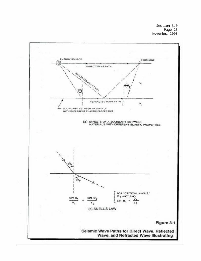
Section 3.0Page 24
November 1993
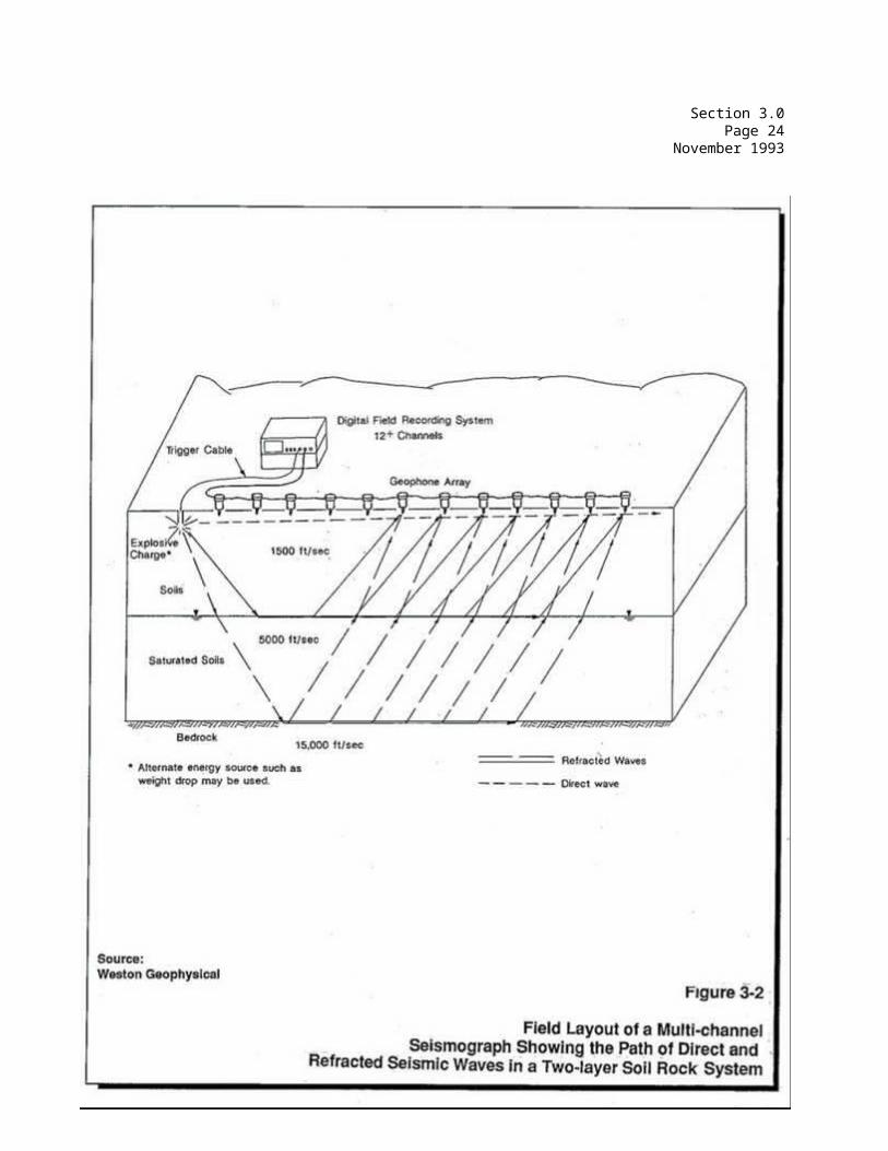
Section 3.0Page 25
November 1993
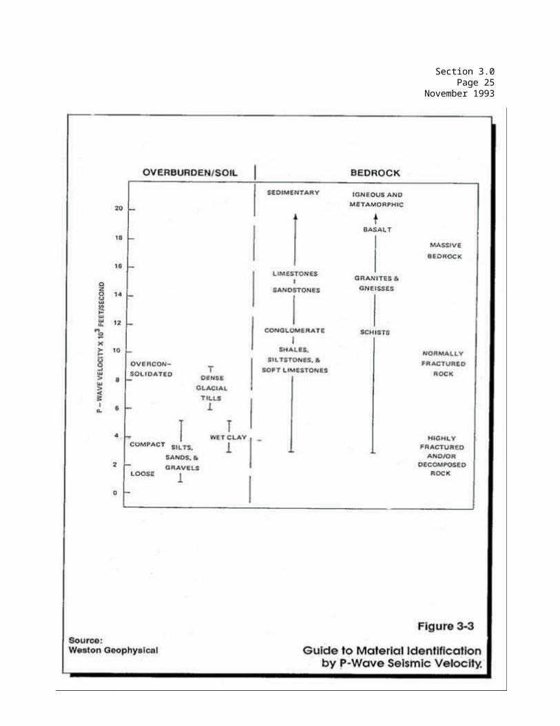
Section 3.0Page 26
November 1993
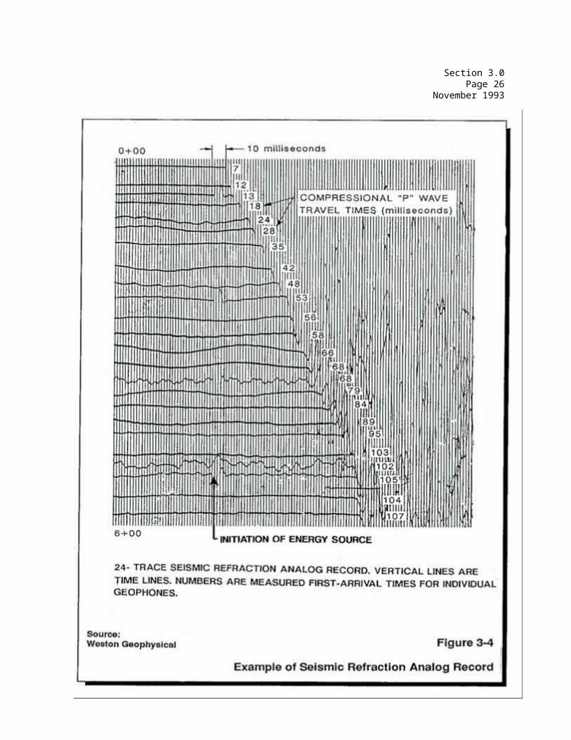
Section 3.0Page 27
November 1993
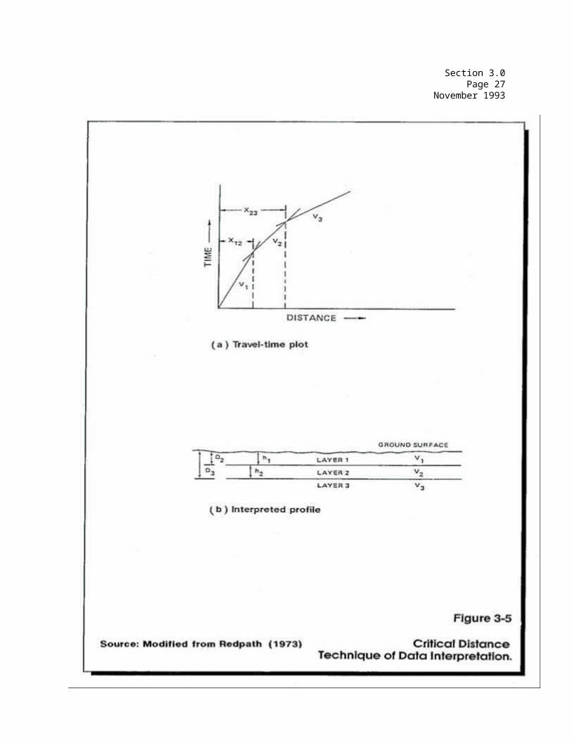
Section 3.0Page 28
November 1993
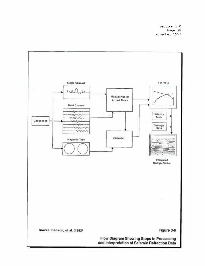
Section 3.0Page 29
November 1993
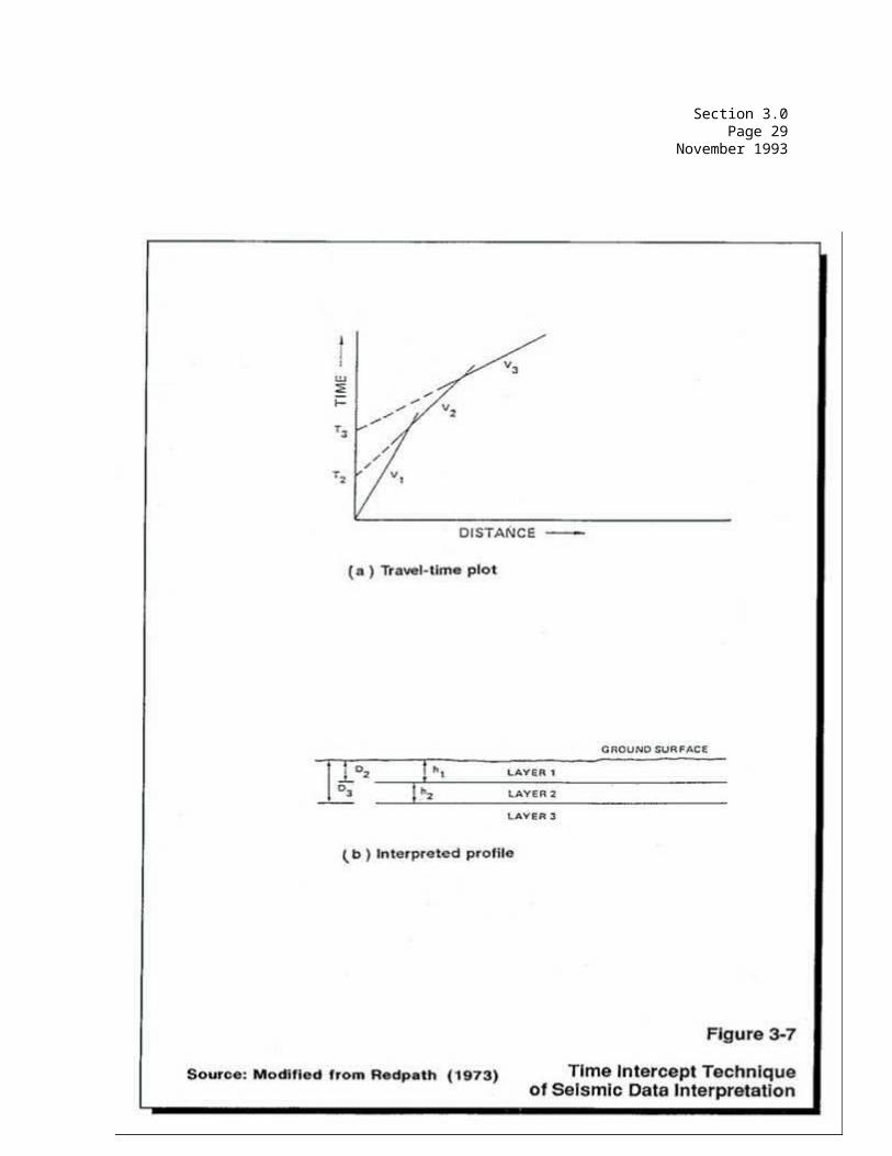
Section 3.0Page 30
November 1993
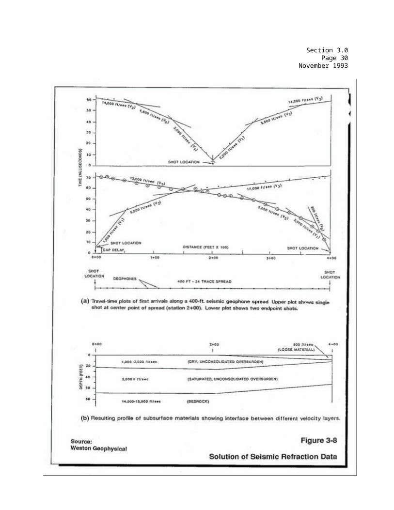
COMMONWEALTH OF MASSACHUSETTS
DEPARTMENT OF ENVIRONMENTAL PROTECTION
STANDARD REFERENCES FOR GEOPHYSICAL INVESTIGATIONS
SECTION 4.0 RESISTIVITY METHODS

Section 4.0Page i
November 1993
SECTION 4.0RESISTIVITY METHOD
TABLE OF CONTENTS
Section Title Page No.
4.1 OVERVIEW......................................... 1
4.2 INTRODUCTION..................................... 2
4.2-1 Electrode Arrays................................. 4
4.2-1.1 Wenner Array..................................... 44.2-1.2 Lee Modification to Wenner Array................. 54.2-1.3 Schlumberger Array............................... 54.2-1.4 Dipole-Dipole Array.............................. 5
4.3 APPLICATIONS .................................... 6
4.4 EQUIPMENT........................................ 7
4.5 FIELD PROCEDURES................................. 8
4.6 INTERPRETATION .................................. 9
4.6-1 Data Analysis.................................... 104.6-2 Presentation of Results.......................... 104.6-3 Interpretation of Results........................ 11
4.7 ADVANTAGES AND LIMITATIONS....................... 12
4.8 GLOSSARY......................................... 13
REFERENCES ................................................. 16
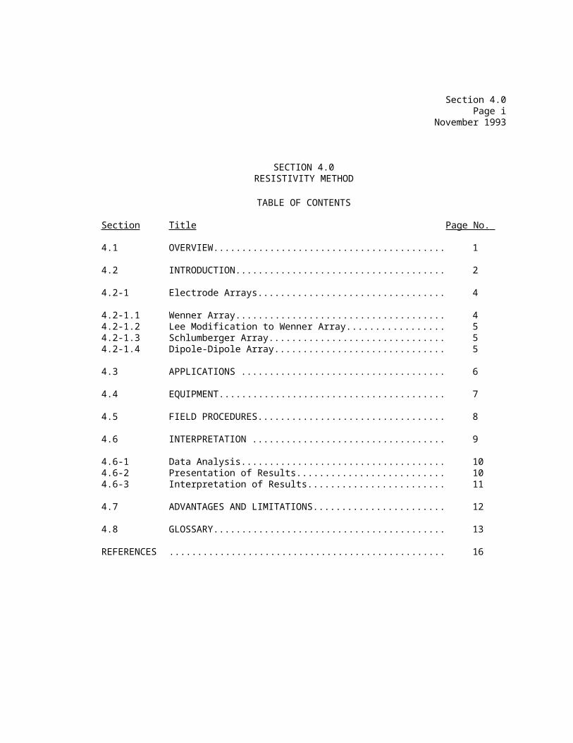
Section 4.0Page ii
November 1993
SECTION 4.0RESISTIVITY METHOD
LIST OF FIGURES
Figure Title Page No.
4-1 Basic Configuration of an Electrical Resistivity Survey............................... 19
4-2 Typical Resistivities for Common Rocks and Soils....................................... 20
4-3 Electrode Arrays Used in Sounding and Profiling Surveys................................ 21
4-4 Example of Wenner Profiling Resistivity Data (a) and Interpretation (b)................. 22
4-5 Example of Wenner VES Data (a) and Interpretation (b)............................... 23
4-6 Example of Dipole-dipole Resistivity Pseudosection Format............................ 24
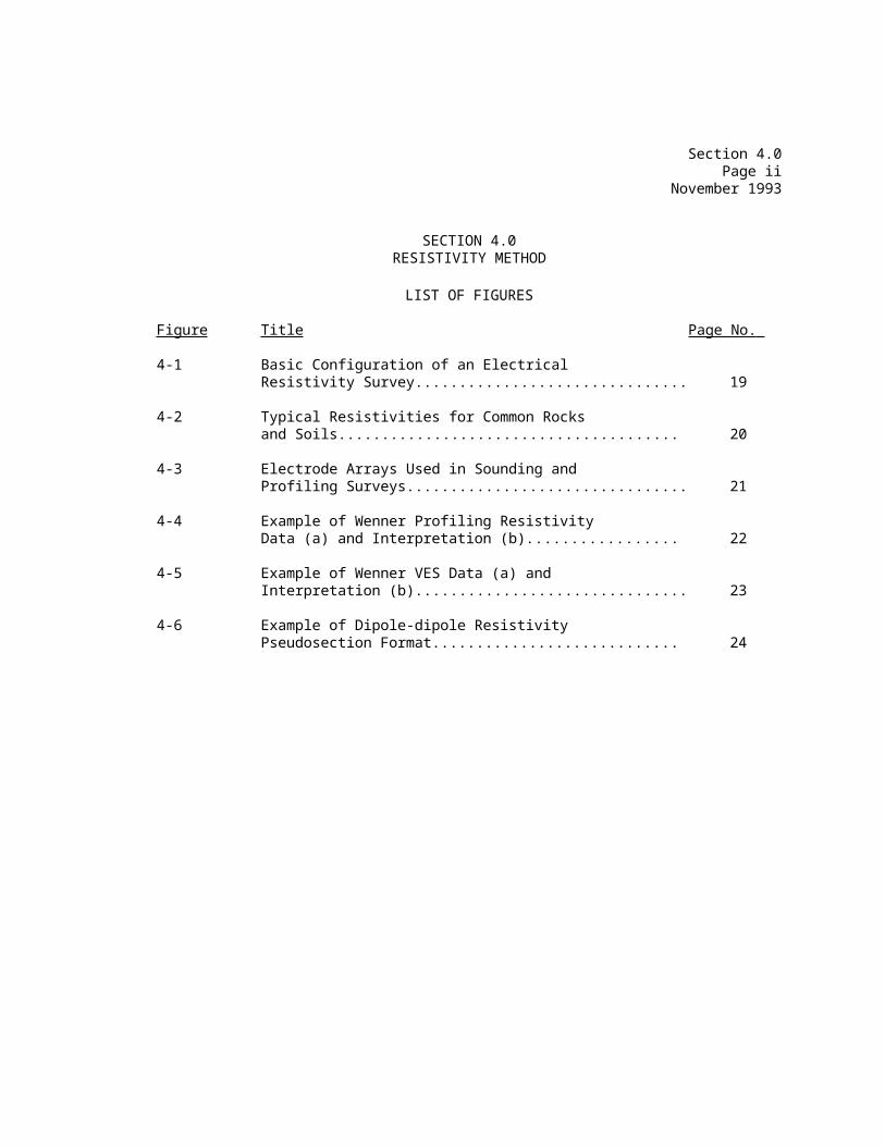
Section 4.0Page 1
November 1993
4.0 RESISTIVITY METHODS
4.1 OVERVIEW
Electrical resistivity surveying is an active geophysical technique that involves applying an electrical current to the earth and measuring the subsequent electrical response at the ground surface in order to determine physical properties of subsurface materials. The general principle of resistivity testing is that dissimilar subsurface materials can be identified by the differences in their respective electrical potentials. Differences in electrical potentials of materials are determined by the application of a known amount of electric current to these materials and the measurement of the induced voltage potentials. Ohm's law states that the voltage (V) of an electric circuit is equal to the electric current (I) times the resistivity (R) of the medium (V=IR). Resistivity surveys are conducted by: 1) applying a known amount of electric current (I) to the earth; 2) measuring the induced voltage (V); and 3) using these two measurements, determining the resistivity (R) of the volume of earth being surveyed.
Resistivity methods usually require that both current inducing and measurement electrodes be pushed or driven into the ground. With connecting wires from the instruments to the electrodes, electrical current is introduced into the ground using the current electrodes, and resistivity measurements are performed using different measurement electrode configurations and spacings. There are a number of standardized testing procedures, some of which are described in detail in this section. Resistivity surveys identify geoelectric layers rather than geologic ones. A geoelectric layer is a layer which exhibits a similar electric resistivity response. A geoelectric layer can, but does not always, correspond to a geologic one. For example, an isotropic homogeneous sand, which is saturated with a fluid exhibiting a single conductivity response, will appear to be a single geoelectric layer. The same sand, if filled with fluid layers containing different conductivities, (i.e., salinities) will appear to be more than one geoelectric layer. The interpretation of resistivity data is therefore best made in conjunction with other geophysical techniques (i.e., seismic refraction) or conventional subsurface investigations (i.e., soil borings).
Historically, resistivity surveys have been used for a number of geologic mapping objectives including groundwater detection, sand and gravel mapping, bedrock depth determination, and other classic geologic exploration exercises. At present, these methods are commonly used to evaluate subsurface conditions as they relate to hazardous waste issues. For example, the resistivity methods have been used to map the extent and direction of migration of conductive groundwater and soil contaminants. The recent development of new survey techniques, known as complex
Section 4.0Page 2
November 1993
resistivity methods, show some promise for mapping non-conductive contaminants, such as petroleum products, which are difficult to detect.
Electromagnetic induction (EM) survey methods (Section 6.0) have generally supplanted resistivity surveys as the method of choice for shallow horizontal resistivity profiling because of EM's ease of use and increased data collection speed. Resistivity methods, however, provide better vertical resolution and are therefore superior to most EM methods for vertical resistivity profiling. Resistivity may also be applicable at sites where interferences from surface metal objects (e.g., fences) and/or power lines make the use of EM surveys impractical.
4.2 INTRODUCTION
Typically, a resistivity survey is conducted by applying an electric current to the earth through two implanted electrodes (current electrodes C1 and C2) and measuring resulting potential difference or voltage drop that occurs between a second pair of implanted measurement electrodes (potential electrodes P1 and P2 as shown on Figure 4-1). An "apparent resistivity" is then calculated using the applied current, measured voltage, and electrode separation data. The resistivity values measured during a field program are known as "apparent" resistivities because the volume of earth encompassed by a survey is often heterogeneous and the measured resistivities are therefore often a composite of resistivities for more than one geoelectric layer. For a single isotropic, homogeneous material, however, the apparent resistivity would equal the true resistivity.
The resistivity (and its reciprocal, electrical conductivity) measured during a survey is a function of the following properties of soil, rock, and groundwater:
o Material composition
o Water content (porosity and degree of saturation)
o Salinity or ion content of the water
o Permeability
o Temperature
Material composition plays a large role in the resistivity of a substance and, in the case of rocks and minerals, can vary widely. For example, graphite has a resistivity of the order of 10-6 ohm-m, whereas some dry quartzite rocks have resistivities of more than 1012 ohm-m (Parasnis, 1962). No other physical property of naturally occurring rocks or soils displays such a wide range of values. The approximate ranges of resistivity for common soil and rock types are shown in Figure 4-2. The ranges of resistivity values for a single material generally indicate
Section 4.0Page 3
November 1993
resistivity variations between dry and water-saturated conditions. Dry sands, gravels, and massive unweathered rock typically exhibit relatively high resistivities (i.e., poor electrical conductors); clays, clayey tills, water-saturated sediments, and weathered rock (chemically broken down to clays) tend to have lower resistivities.
The water content (which is a function of material porosity and the amount of pore saturation) of a material is the greatest single factor controlling the electrical characteristics of subsurface geology. Most soil and rock materials are relatively poor electrical conductors (i.e., exhibit high resistivities) compared with groundwater. An applied electric current is conducted almost entirely by the water in the pore spaces or fractures of soil or rock rather than by the soil or rock alone. This also applies to the unsaturated (vadose) zone, because in general there is some moisture in unsaturated media. Dry material yields higher values of resistivity; accordingly, it is more difficult for electricity to pass through layers such as dry sands or gravels. Conversely, if materials are saturated (especially in the case of clays) electricity can pass through the layering more easily and such layers are referred to as good electrical conductors (low resistivity materials).
Salinity (or ion content) also plays an important role in the resistivity of a material. If salts are present (i.e. nearby ocean environments, landfill leachate plumes, or areas adjacent to roadways kept clear of ice by the practice of spreading salt) recorded data will reflect abnormally high conductivity values for the subsurface material. On the other hand, pure (distilled) water is non-conductive, however, most groundwater contains some dissolved salts and hence is somewhat conductive.
Formation permeability (as well as resistivity) is a function of, and is directly proportional to, the interconnectedness of the formation pores. The geometrical arrangement of the pore spaces may make formation resistivity anisotropic. The vertical resistivity of a geoelectric layer, which would be more likely to affect a surface resistivity measurement, could therefore be different than the horizontal resistivity, which would be measured by a borehole resistivity survey (see Section 10-3.5).
The temperature of a formation will also affect the electrochemical activity of groundwater and will therefore also affect conductivity of the medium. Fluid conductivity is directly proportional to the temperature. In most cases, however, subsurface temperature variation is minimal and therefore conductivity corrections are not necessary.
A basic principal of resistivity surveys is: the greater the distance between the current and the measurement electrode, the greater the depth of investigation. Widely spaced traverses or soundings are used for reconnaissance surveys or for delineation of large targets (horizontally extensive clay or gravel layers). Closely spaced data are required for identification of localized features such as discrete zones of leachate
Section 4.0Page 4
November 1993
migration, etc.
Resistivity measurements are commonly used to delineate either changes in resistivity with depth or lateral variations in resistivity. These applications are known respectively as:
o Vertical electrical soundings (VES)
o Horizontal profiling
VES surveys, which determine vertical resistivity changes, employ variable electrode spacings. VES surveys are used to identify geoelectrical layering in soil and rock. These data are often used to identify: the groundwater table; clay layers; the bedrock surface; and to select optimum electrode spacings for horizontal profiling surveys.
For horizontal profiling, which determines lateral resistivity changes at a fixed depth of investigation, the current measurement electrode spacings are kept constant. Horizontal profiling is used to identify lateral resistivity variations in a survey area. Horizontal profiling can be used to detect conductive groundwater plumes, landfill limits, geologic contacts, and sink holes (often present in limestone lithology). 4.2-1 Electrode Arrays
A variety of electrode arrays are used for resistivity surveys. The most common ones will be discussed in this section and are presented on Figure 4-3. The most commonly used electrode arrays - (On Figure 4-3, "C1" and "C2" are the two current electrodes, "P1", and "P2" are the two potential electrodes, "V" is voltage, "I" is current, and "ρa" is apparent resistivity.) are:
o Wenner
o Lee modification of Wenner
o Schlumberger
o Dipole-dipole
All of the above arrays employ both current inducing and measurement electrodes. Differences between the arrays consist of variations in electrode spacing and relative position. Each array is designed to measure the induced electrical (potential) field differently and is more suited to either the horizontal or vertical survey applications.
4.2-1.1 Wenner Array
The Wenner array is constructed by placing four equally spaced electrodes
Section 4.0Page 5
November 1993
in a straight line. One current inducing electrode is placed at each end of the survey line and the two measurement electrodes are placed in the center. The data collected using the Wenner array produces an average of the induced potential present between the current electrodes. The Wenner array is suitable for VES surveys, but is less applicable to horizontal profiling because data averaging reduces sensitivity to lateral variations in resistivity.
4.2-1.2 Lee Modification to Wenner Array
The Lee modification of the Wenner array involves the addition of a third potential measurement electrode halfway between P1 and P2 (see Figure 4-3). The Lee modification increases the applicability of the Wenner array to horizontal resistivity profiling. Three potential measurements are taken, using electrodes P1 - P2 (normal), P1 - P0 (Lee left), and P2 - P0
(Lee right). Apparent resistivities are calculated for the Lee left and right measurements. If the left and right measurements do not each equal one-half of the normal measurement, then a lateral variation in resistivity exists in the vicinity of the potential electrodes.
4.2-1.3 Schlumberger Array
The Schlumberger and Wenner arrays have some similarities. Both can be used for profiling or VES surveys, and both have a maximum depth of investigation related to the current electrode separation (approximately one-third of the Wenner "a-spacing" or one-ninth of the Schlumberger current electrode separation).
In the Schlumberger array, the potential measurement electrodes are relatively close together with respect to the current electrode spacing. The Schlumberger array's performance is comparable to that of the Wenner array for VES applications, but has greater sensitivity in horizontal profiling. Generally, a Schlumberger VES survey is simpler to operate than a Wenner VES survey, because less electrode movement is required. At sites where many local variations in resistivity occur near the ground surface, Schlumberger results may be more accurate because the potential electrodes are kept in the same position/material for several readings. (Wenner results in this scenario will be more variable because the potential electrodes would be placed in different media for each reading.)
4.2-1.4 Dipole-Dipole Array
A dipole-dipole array differs from the three previously discussed arrays in that the two current electrodes are grouped together (this grouping is called a dipole). The two measurement electrodes are grouped together (as another dipole), but are not between the current electrodes (see Figure 4-3[III]). The distance (a) between the two dipoles is normally
Section 4.0Page 6
November 1993
set to be much greater than the distance between the electrodes of each dipole (b). Four basic geometric arrangements, azimuthal, radial, parallel, and equatorial have been developed for exploration purposes. The parallel dipole-dipole array configuration can be placed in a straight line as is shown in Figure 4-3(III) to help simplify data computation (the straight line arrangement has removed the angle correction component from the algorithm shown in Figure 4-3[III]. The dipole-dipole array is more sensitive to lateral changes in resistivity than the Wenner or Schlumberger arrays, but less sensitive to changes with depth (VES).
4.3 APPLICATIONS
Contrasts in resistivity for some geologic materials (see Figure 4-2) make resistivity surveying a valuable technique for many applications including:
o Groundwater depth determination
o Landfill boundary determination
o Delineation of conductive contaminant plumes and/or buried wastes
o Location of fresh/salt water interfaces
o Detection of a perched water table
o Distinguishing bedrock and sediment lithologic types and contacts
o Identification of zones of weathered bedrock, fractures, and possibly solution cavities
Examples of resistivity applications, including identification of buried stream channels and clay layers, and mapping the groundwater table may be found in Zhody et al. (1974) and Yazicigil and Sendlein (1982).
Schlumberger profiling measurements have greater sensitivity to lateral resistivity changes and Schlumberger VES data collection produces less error due to heterogeneous near-surface materials than Wenner arrays.
Wenner measurements are more accurate at sites where small potential voltages are induced, including sites with low resistivity (high conductivity) clays.
Either Wenner or Schlumberger arrays may be used for both reconnaissance and detailed measurements by varying the spacing between profile traverses or sounding locations.
Section 4.0Page 7
November 1993
A dipole-dipole survey is better-suited to locating discrete features (buried metal, igneous dikes, solution cavities), than for identification of soil and rock layering. The dipole-dipole survey method would be an appropriate choice for mapping the direction and orientation of discrete bedrock fractures if a Very Long Frequency (VLF) method (Section 6.0) could not be used.
Resistivity surveys have occasionally been applied to the problem of detecting electrically resistive contaminants (i.e., petroleum hydrocarbons), however, such surveys are generally not suited to this application. Successful applications of resistivity in organic contaminant identification requires (1) conductive contaminants (landfill leachate, chlorides, iron oxides, dissolved nitrates and salts); or (2) a layer of organic product (hydrocarbons including gasoline, PCBs) several feet thick which displaces the groundwater table; however, free floating product may have electrical properties quite similar to non-saline groundwater.
4.4 EQUIPMENT
Basic field equipment needed for resistivity surveying includes:
o two current electrodes
o two potential electrodes (three for Lee modification of Wenner array)
o insulated connecting cables
o non-conductive fiberglass measuring tapes
o source of electric current
o voltage measurement device
Steel and copper-clad steel are common electrode materials, although other metals may be used. Electrodes of dissimilar metals should not be used during a survey (e.g., three steel electrodes and one aluminum electrode) because unusually large self-potentials can be generated.
Resistivity instrumentation includes a variety of designs with widely varying capabilities. Advantages and limitations of four popular designs are discussed in this section.
The simplest resistivity instruments are known as "DC" (direct current) devices. They apply a direct current to the earth and measure the resulting DC potential with a high-impedance (at least 1 x 10⁶ ohm) volt meter. Because SP (self-potential) voltages can adversely affect the accuracy of simple DC resistivity measurements, these instruments usually contain a "nulling" or "balancing" circuit to remove the SP effect.
Section 4.0Page 8
November 1993
Although SP constitutes a form of noise in a resistivity survey, SP measurements can also be used as a geophysical exploration technique (see Section 5.0 of these Standard References). If SP is varying rapidly in the area of investigation then its effect is nearly impossible to remove or compensate; for this reason, simple DC resistivity measurements are not suitable for all field areas; see Section 5.1 for a discussion of SP sources.
A more versatile resistivity meter is known as the low-frequency "AC" (alternating current) type. This instrument uses a sinusoidal applied current, usually of only a few hertz, to avoid some of the interferences caused by SP. Both the DC and low-frequency AC meters are best-suited for relatively shallow investigations, with depths of investigation less than about 100 feet, in soils that are neither highly conductive nor highly resistive. These limitations are imposed by the small battery-powered current transmitters used. Current output of these units is measured in tens of milliamps at less than one thousand volts.
More powerful resistivity equipment, utilizing sinusoidal AC or square-wave DC transmitters powered by portable electric generators is also available. These units often have a transmitter and receiver mounted in separate housings to provide greater versatility and to minimize electrical interference between the transmitting and receiving circuits. They also have the capability of producing up to tens of amperes of current at several thousand volts, sufficient for surveys in highly resistive or conductive media at maximum depths much greater than battery powered instruments.
Recent innovations in electronics design have resulted in a resistivity meter that fills a niche between the standard battery and generator powered AC instruments. These units are also battery-powered, but produce electric currents with unique waveforms. Voltage measuring circuits in these devices are designed to recognize the specific waveform produced by the transmitter, thus enabling measurement of weak potentials in somewhat noisy conditions. Signal enhancement (summing of a few voltage measurements) is usually offered with these instruments and also contributes to improved resolution. This type of resistivity meter is capable of operation in more resistive or conductive media than the low-frequency AC meters, and can also be used to investigate deeper structures.
4.5 FIELD PROCEDURES
Verification of the equipment's operating condition, by obtaining repeating resistivity measurements at a known location prior to conduct of field work, is advised.
Careful planning is important when conducting a resistivity survey. Thin layers, or targets of limited lateral extent, may be undetectable because the measured potentials integrate the effects of a large volume of
Section 4.0Page 9
November 1993
material. This difficulty can be reduced if the minimum size and resistivity contrast of the expected target is known before the field measurements are begun. Numerical modeling can then be performed to select the most effective electrode array and spacing to identify the desired target. This approach is particularly effective in planning VES and dipole-dipole surveys.
Parallel survey lines should be tied together with a perpendicular line, or by using another geophysical technique such as EM or seismic. To minimize the interference caused by metal fences or other cultural features, electrode arrays should be placed perpendicular to metal fences or other linear conductive objects to more readily identify their influence. Topographic effects are minimized if the electrodes are maintained at nearly the same elevation.
A VES survey is best performed along hillside contours (at the same elevation), rather than parallel to the hill slope.
Field procedures involve placing electrodes at the intended separations, connecting the electrodes to the transmitter and receiver, and obtaining current and potential measurements. Electrode locations should be determined with non-conductive measuring tapes to avoid providing an alternative path for the applied current. Fiberglass tapes are commonly used. Most resistivity surveys are performed with metal electrodes which are driven one to three feet into the ground. If needed, water can be poured around each electrode to decrease the resistance at the contact zone between the electrode and the earth materials. (Copper sulfate solutions have historically been used to improve electrode contact, but any local water source is usually sufficient.) Electrodes are connected to the resistivity instrumentation using insulated wire.
At sites with strong self-potential noise effects, use of DC resistivity instrumentation may necessitate non-polarizing electrodes. These special electrodes are commonly of the porous-pot type, consisting of an unglazed ceramic pot containing a metal electrode and a saturated electrolytic solution. The electrolytic solution must contain a salt of the same metal as the central electrode (e.g., a solution of copper sulfate is often used with a copper electrode). The porous pot is placed on the ground surface, and electrical contact with the earth is achieved by seepage of the electrolytic solution through the porous ceramic.
Quality assurance (QA) is important in resistivity field procedures. This QA effort entails careful measurement of electrode positions and the checking of resistances across potential and current electrodes to ensure good contact with the earth. Plotting calculated apparent resistivities in the field, to ensure good data quality, is advised. Instrument calibration is not usually of concern because the equipment is calibrated by its manufacturer.
4.6 INTERPRETATION
Section 4.0Page 10
November 1993
4.6-1 Data Analysis
Analysis of resistivity data involves different procedures for horizontal profiling, VES surveys, and dipole-dipole surveys. Horizontal profiling data is contoured or plotted on linear graph paper, with apparent resistivity values on the y-axis and distance along the traverse on the x-axis. The contour map or profiles are then examined for relative variations in resistivity which may be indicative of the intended target body. An example of Wenner profiling data is provided on Figure 4-4.
Wenner and Schlumberger VES data are plotted on log-log graph paper with the apparent resistivity values on the y-axis and Wenner a-spacings or Schlumberger current electrode separations (times one-half) on the x-axis (Figure 4-5).
Computer-aided VES modeling can be performed in two manners, forward modeling and inverse modeling. Forward modeling entails computation of theoretical resistivity values from a layer thickness/resistivity model supplied by the interpreter. Agreement between the field and theoretical curves in the model is obtained by subsequent trial and error refinement of the layer parameters (thicknesses and resistivities). As is the case with most computer models, any known site conditions such as depths to groundwater or significant stratigraphic horizons can greatly increase the accuracy of modeled resistivity interpretations. Boring or test pit logs, if available, should be used to confirm the resistivity modeling results. Inverse VES modeling also begins with computation of theoretical resistivity values from layer parameters supplied by the interpreter, but refinement of the layer parameters is automatically performed by the computer code. The final product of an inverse modeling program is a set of layer parameters and a corresponding theoretical curve which provide the best possible fit to the field data. This "numerically correct" interpretation must be examined by a geologist or geophysicist to ensure that the model is geologically reasonable. Again, actual field data from a boring or test pit should be used to check the model. Dipole-dipole resistivity analysis is considerably different from horizontal profiling or VES analysis. Dipole-dipole data are displayed in a two-dimensional pseudosection format (Figure 4-6), and the analysis is thus performed by two-dimensional numerical modeling. An example of finite-element modeling of dipole-dipole data may be found in Rijo (1977). The complexity of this finite-element modeling requires the use of the use of a trained interpreter and a mini-computer (at present no analytical programs for this method have been written for personal computers). These analytical restrictions will limit the number of geophysicists willing and/or qualified to perform detailed quantitative dipole-dipole interpretation.
4.6-2 Presentation of Results
Section 4.0Page 11
November 1993
Horizontal profiling data are contoured or presented as linear-linear plots of apparent resistivity versus distance along a traverse. The line stationing notation (in hundreds of feet) listed in Figure 4-4 refers to the distance along a traverse from an arbitrary origin point (0+00). An example of the profile plotting technique is provided on Figure 4-4.
VES data are plotted on log-log graphs with apparent resistivity values on the y-axis and Wenner a-spacings or the Schlumberger current electrode separations (times one-half) on the x-axis. See Figure 4-5 for an example. Layer parameters used in VES modeling, i.e., layer thicknesses and resistivities, must be included with each VES plot, as shown on Figure 4-5.
Dipole-dipole data are shown as pseudosection plots, usually with resistivity values contoured (see Figure 4-6). A cross section of the inferred geologic model should accompany the pseudosection plot.
4.6-3 Interpretation of Results
Interpretation of resistivity data entails comparing resultant ranges of resistivity values with natural earth materials or manmade objects likely to be present. Horizontal profiling data and VES modeling results are directly indicative of the resistivities of the materials encountered: higher resistivity values represent more electrically resistive materials (such as sands or gravels). Figure 4-4 shows Wenner horizontal profiling data (collected using fixed electrode spacing) over a localized zone of anomalously low resistivity soil. Figure 4-5 shows Wenner resistivity vertical sounding data (collected using increasing electrode spacing) over a clay seam, known to be present by borehole information, that occurs between more resistive soil layers. Until several years ago, interpretation would have next been accomplished by comparison of the field data with published master curves. Examples of the curves and their use may be found in Orellana and Mooney (1966), Keller and Frischknecht (1966), Dobrin (1976), Telford et al. (1976), Van Nostrand and Cook (1966), and Zhody et al. (1974). This technique is slow and limited in application because curves are available only for two and three layer cases at a few resistivity contrasts. Currently, VES interpretations are performed using a computer and the linear filter algorithm described by Ghosh (1971a and 1971b) and Koefoed (1979). This algorithm operates very quickly on any computer, from a mainframe to a laptop, and provides greater accuracy and versatility than is possible with manual curve matching techniques. A contractor should clearly identify the modeling technique used in the interpretation.
Dipole-dipole interpretation is more subjective, and requires an experienced interpreter. The complexity of dipole-dipole interpretation arises from the lack of correspondence between a dipole-dipole pseudosection and the actual resistivities of the earth materials investigated. As a simple example, a low-resistivity vertical dike will
Section 4.0Page 12
November 1993
produce a dipole-dipole anomaly in the shape of an inverted letter "V" (Figure 4-6). Although the dike has material of low resistivity, the anomaly will contain both low and high resistivity values which could be misinterpreted by inexperienced personnel.
Correlation of resistivity data with other geophysical data sets, borehole geologic logs, or borehole cores and samples, is necessary to more accurately identify the materials or structures inferred from the resistivity results. Estimates of layering thicknesses from resistivity modeling typically have to be compared with seismic refraction or geologic data because of the imprecision inherent in resistivity layer calculations. The imprecision is caused by the non-uniqueness of resistivity data: many different models can produce theoretical curves which nearly fit the field data. A knowledgeable interpreter is thus needed to successfully integrate the resistivity results with other data, including geologic information regarding the site of interest.
All reports must include a statement of the field and computer methods used, including calibrations and correlations with other geologic and geophysical data.
4.7 ADVANTAGES AND LIMITATIONS
Advantages
Some of the advantages of resistivity surveying include:
o The portability of the equipment.
o The potential for in-field data analysis using portable computers with horizontal profiling and VES surveys.
o Can provide stratigraphic data when frozen surface soils preclude the use of seismic refraction.
o Direct detection, in some instances, of conductive contaminant plumes. In addition to the detection, delineation of the lateral and vertical extent of the plume can also be accomplished.
Resistivity data are well-suited for correlation and verification by a variety of geophysical techniques and/or test borings. Correlative geophysical techniques for some of the applications listed below include seismic refraction, electromagnetic terrain conductivity, ground penetrating radar (GPR), and magnetometry.
Limitations
Equally important are the limitations inherent in resistivity surveying,
Section 4.0Page 13
November 1993
as reviewed below. Knowledge of these limitations is critical to avoid misapplication of the resistivity technique.
o The resistivity surveying methods can be carried out only in media which are neither extraordinarily conductive or resistive. If electrodes are placed in very conductive material, (e.g., a salt marsh) then the applied current flow may become trapped in the conductive layer. A bedrock layer underlying the marsh could remain undetected because virtually none of the current would pass through the marsh into the rock.
o In very resistive materials, such as talus, resistivity surveying often cannot be performed because poor electrode contact prevents introduction of electric current into the earth. Marginal cases may be aided by wetting the electrodes to decrease earth resistance, but in severe cases the resistivity method must be replaced with another technique.
o Another limitation is the size of a target body which can be detected by resistivity surveys. Thin layers, or targets of limited lateral extent, may be undetectable because the measured potentials integrate the effects of a large volume of material.
o Numerical modeling solutions may not be unique, and the more layers present the more difficult an accurate solution becomes.
o Because this technique measures geoelectric layers rather than geologic ones, in the absence of correlating data (e.g., boring logs) incorrect stratigraphic conclusions can be drawn.
o Differentiation between highly conductive materials (i.e., clay or salt water versus contamination plumes) may not be possible.
o Cultural interference is another serious limitation of resistivity surveying. Interference from powerlines, pipelines, and metal fences can be minimized by orienting electrode arrays perpendicular to them. The same approach can be used with underground utilities, but in general cultural interference is best avoided altogether.
o A resistivity horizontal profiling survey is more labor intensive and time consuming than an EM survey (Section 6).
4.8 GLOSSARY
Section 4.0Page 14
November 1993
Algorithm - A mathematical rule or procedure for solving a problem.
Anisotropy - Having physical properties which vary with the orientation of measurement.
Dipole-dipole - A configuration of electrodes with the current and potential electrodes emplaced as separated pairs.
Electrical Potential - A term that refers to the voltage measured between one pair of electrodes.
Finite-element modeling - A numerical method of approximating a solution to differential equations.
Geoelectric Layer - A stratigraphic layer or layers which exhibit the same electrical resistivity. A geoelectric layer can include materials of different geologic age and/or different lithologic composition. Conversely, a lithologically homogeneous material containing fluid layers with different conductivities would appear as multiple geoelectric layers.
Hertz - A unit of frequency. One hertz equals one cycle per second.
Homogeneous - Having the same physical properties regardless of the location of measurement.
Impedance - The apparent resistance to the flow of alternating current; analogous to resistance in a direct current circuit.
Isotropy - Having physical properties which are uniform regardless of the measurement orientation.
Lithology - The description of rocks based upon its characteristics, such as color, composition, and grain size.
Milliamp - A unit of electric current flow, equal to one thousandth of an ampere.
Pseudosection - A plot of apparent resistivity measurements made along a line at various electrode separations. It conveys the variation of apparent resistivity with location and penetration depth but cannot be directly converted into resistivity distribution.
Sinusoidal - An adjective describing a curve in the pattern of a sine function (mathematics).
Sounding - Measurement of geoelectrical properties as they vary with depth.
Square wave - A waveform consisting of alternating positive and negative
Section 4.0Page 15
November 1993
portions.
VES - Vertical electrical sounding - A mode of resistivity exploration wherein electrodes are spaced at progressively greater distances to permit penetration of electric current and detection of deeper layering.

Section 4.0Page 16
November 1993
REFERENCES
Benson, R. C., Glaccum, R. A., and Noel, M. R., 1982, Geophysical techniques for sensing buried wastes and waste migration: USEPA #68-03-3050.
Dobrin, M.B., 1976, Introduction to geophysical prospecting (2nd ed.): New York, NY, McGraw-Hill, 446 p.
Ghosh, D.P., 1971(a), The application of linear filter theory to the direct interpretation of geoelectrical resistivity sounding measurements: Geophysical Prospecting, v. 19, no. 2, p. 192-217.
____, 1971(b), Inverse filter coefficients for the computation of apparent resistivity standard curves for a horizontally stratified earth: Geophysical Prospecting, v. 19, no. 4, p. 769-775.
Keller, G.V., and Frischknecht, F.C., 1966, Electrical methods in geophysical prospecting: Elmsford, NY, Pergamon Press, 523 p.
Koefoed, O., 1979, Geosounding principles, 1 -Resistivity sounding measurements: New York, NY, Elsevier, 276 p.
Orellana, E., and Mooney, H.M., 1966, Master tables and curves for vertical electrical sounding over layered structures: Madrid, Spain, Interciencia, 150 p. (Available from: U.S. Army Corps of Engineers Waterways Experiment Station, Vicksburg, MS, 39180).
Rijo, L., 1977, Modelling of electrical and electromagnetic data: Ph.D. dissertation, University of Utah, Department of Geology and
Geophysics, 242 p.
Telford, W.M., Geldart, L.P., Sheriff, R.E., and Keys, D.A., 1976, Applied geophysics: New York, NY, Cambridge University Press, 860 p.
U.S.Army Corps of Engineers, 1979, Geophysical exploration: Engineer Manual No. EM-1110-1-1802, Vicksburg, MS, 313 p.
Van Nostrand, R.G., and Cook, K.L., 1966, Interpretation of resistivity data: U.S. Geological Survey Professional Paper 499, 310 p.
Van Blaricom, R., 1980, Practical geophysics for the exploration geologist: Spokane, WA, Northwest Mining Association, p. 45.
Section 4.0Page 17
November 1993
Yazicigil, H., and Sendlein, L.V.A., 1982, Surface geophysical techniques in groundwater monitoring, Part II: Groundwater Monitoring
Review, v. 1, no. 1, p. 56-62.
Zohdy, A.A.R., Eaton, G.P., and Mabey, D.R., 1974, Application of surface geophysics to groundwater investigations: U.S. Geological
Survey, Techniques of Water-Resources Investigations, Book 2, Chapter D1, 116 p.

Section 4.0Page 18
November 1993
SECTION 4.0RESISTIVITY METHOD
LIST OF FIGURES
Figure Title Page No.
4-1 Basic Configuration of an Electrical Resistivity Survey............................... 19
4-2 Typical Resistivities for Common Rocks and Soils........................................ 20
4-3 Electrode Arrays Used in Sounding and Profiling Surveys................................ 21
4-4 Example of Wenner Profiling Resistivity Data (a) and Interpretation (b).................. 22
4-5 Example of Wenner VES Data (a) and Interpretation (b)............................... 23
4-6 Example of Dipole-dipole Resistivity Pseudosection Format............................. 24
Section 4.0Page 19
November 1993
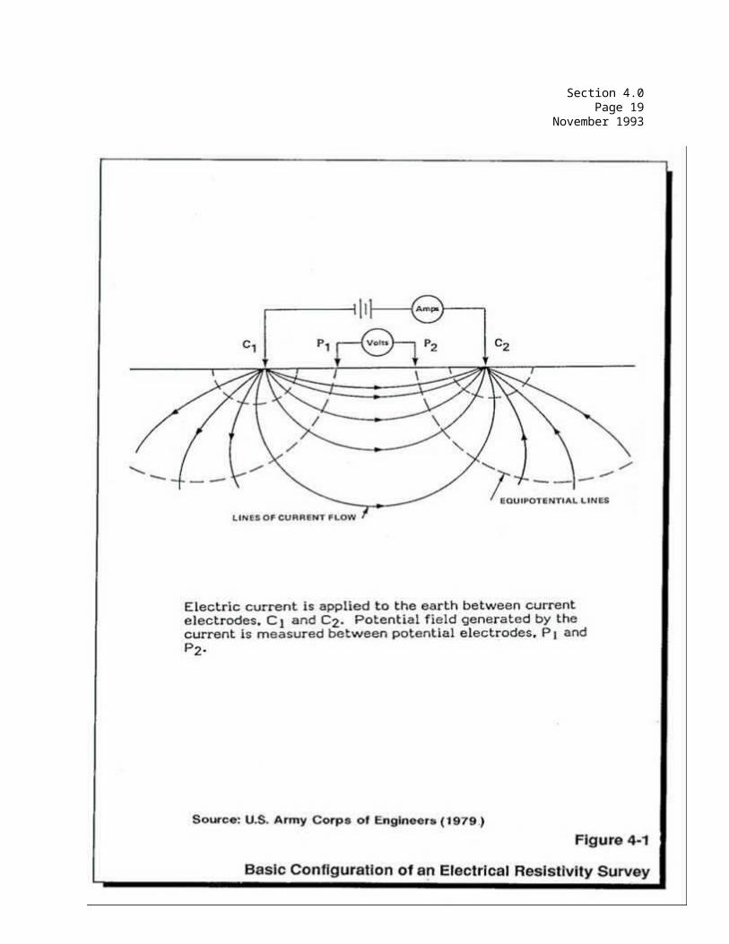
Section 4.0Page 20
November 1993
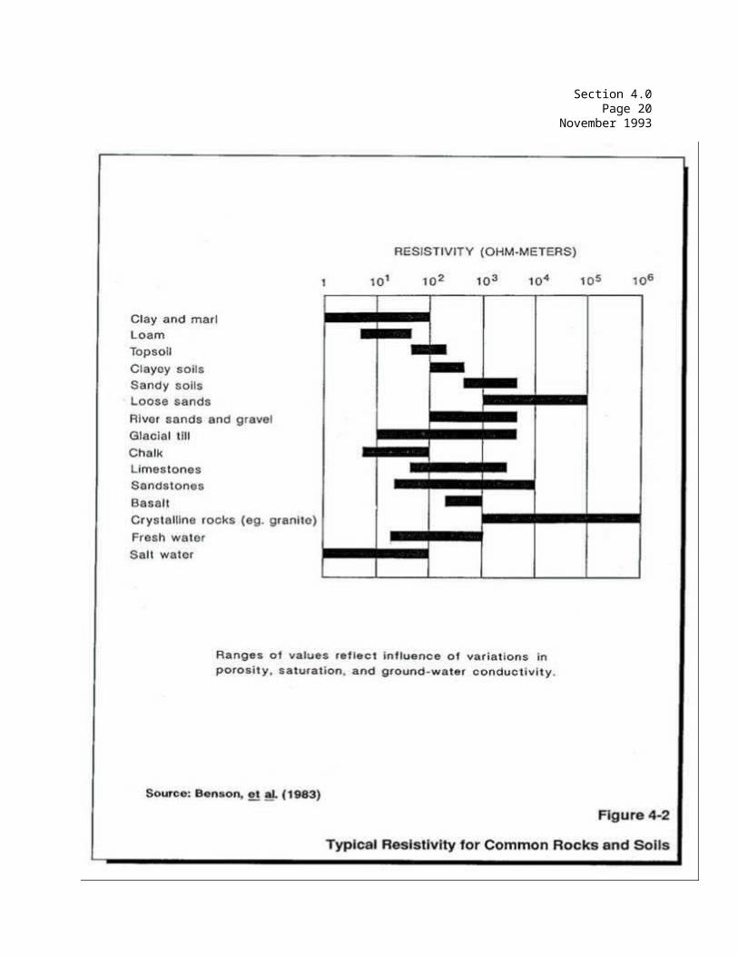
Section 4.0Page 21
November 1993
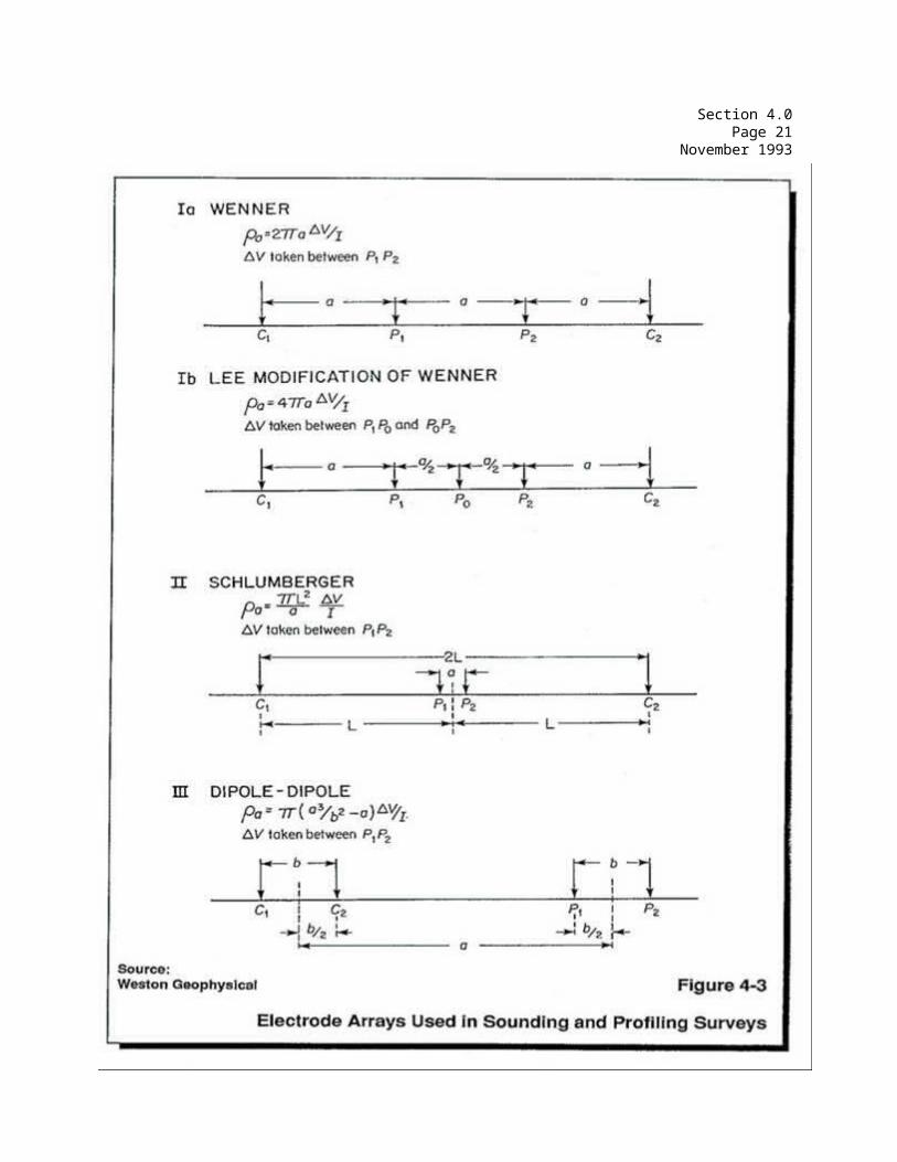
Section 4.0Page 22
November 1993
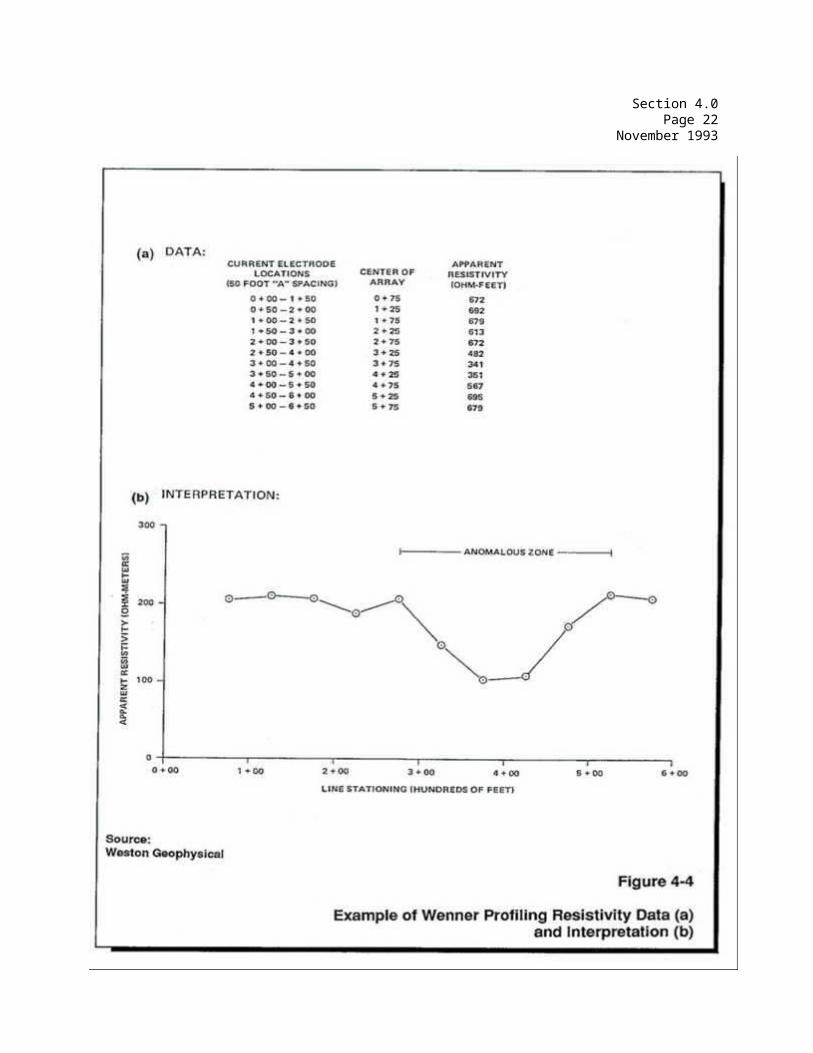
Section 4.0Page 23
November 1993
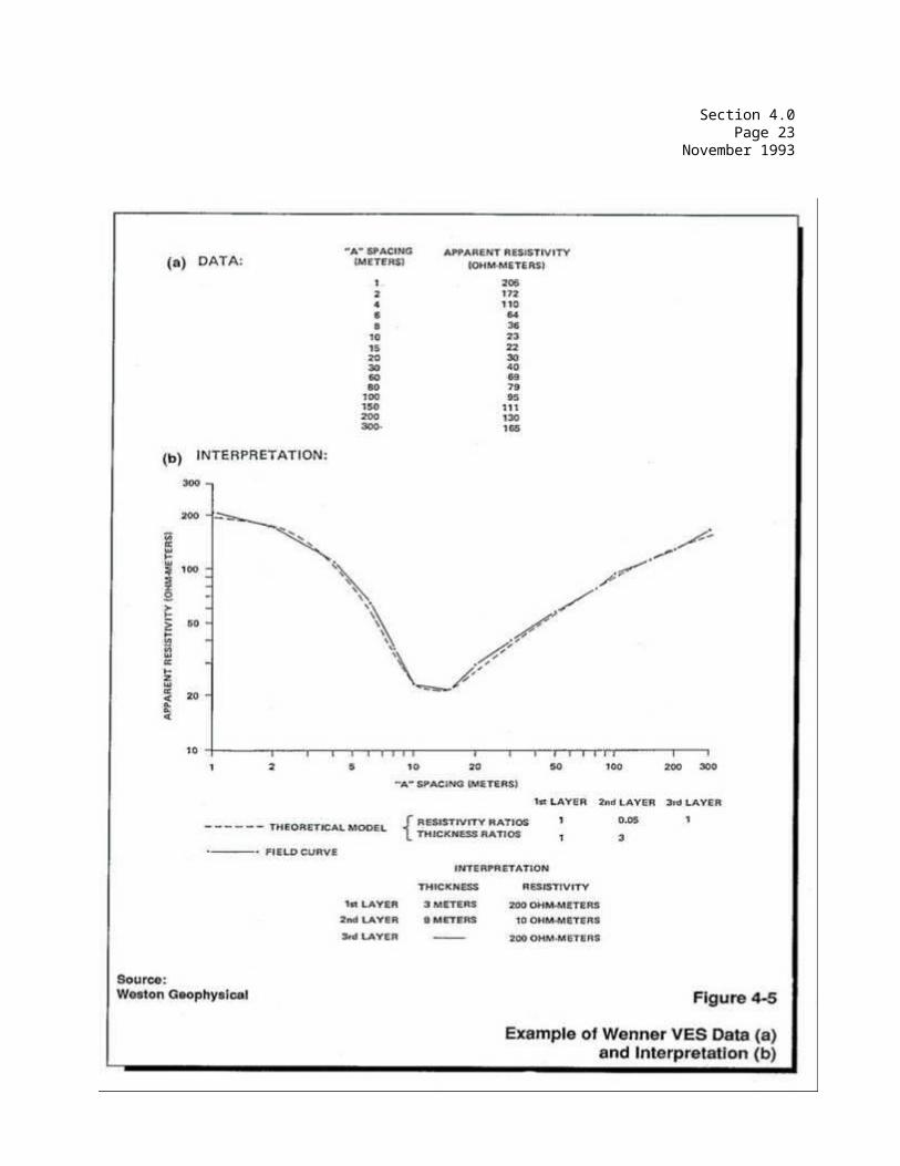
Section 4.0Page 24
November 1993
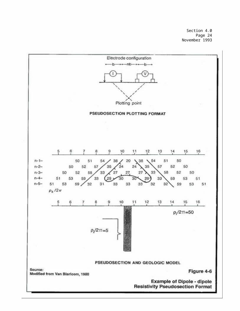
COMMONWEALTH OF MASSACHUSETTS
DEPARTMENT OF ENVIRONMENTAL PROTECTION
STANDARD REFERENCES FOR GEOPHYSICAL INVESTIGATIONS
SECTION 5.0 SELF-POTENTIAL METHOD
Section 5.0Page i
November 1993
SECTION 5.0SELF-POTENTIAL METHOD
TABLE OF CONTENTS
Section Title Page No.
5.1 OVERVIEW.........................................1
5.2 INTRODUCTION.....................................1
5.3 APPLICATIONS.....................................2
5.4 EQUIPMENT........................................2
5.5 FIELD PROCEDURES.................................3
5.6 INTERPRETATION...................................4
5.6-1 Data Analysis....................................45.6-2 Presentation of Results..........................45.6-3 Interpretation of Results........................4
5.7 ADVANTAGES AND LIMITATIONS.......................4
5.8 GLOSSARY ........................................5
REFERENCES .................................................6
LIST OF FIGURES
Figure Title Page No.
5-1 Self Potential Measurements for Dam and Reservoir Seepage Detection......................8
(a) Data Profile Across Dam(b) Field Layout of Electrode Line, A-A'
5-2 Self Potential Measurements for Groundwater Migration Studies................................9
(a) SP Data Plot(b) Geologic Cross-Section
Section 5.0Page 1
November 1993
5.0 SELF-POTENTIAL METHOD
5.1 OVERVIEW
The self-potential (SP) survey method is a passive geophysical technique, which measures extremely small, naturally occurring voltage variations in the earth. The technique is based on the observation that when certain materials are in contact with either a different material (e.g., buried iron next to buried copper) or a localized change in the condition of the same material (e.g., interface of saturated and unsaturated condition), an electrical current is created. This current is readily detectable with inexpensive, portable voltage measuring instrumentation.
The technique is simple to operate, consisting of a series of measurements of electric potential (voltage) across two electrodes which are in contact with the ground and spaced at varying distances.
The most relevant application of this method to environmental investigations is the tracing of shallow leachate seepage zones when such zones are known to exist.
Given the small size of the naturally occurring voltage differentials (measured in thousandths of volts), the SP method is extremely sensitive to man-made electrical interferences.
Although the technique is receiving increased attention for groundwater contamination assessment, the reliability and applicability of this methodology are inconclusive at this time.
5.2 INTRODUCTION
The self-potential method used in land surveys is similar to the SP technique that is covered in Section 10.0 as one of the borehole geophysics methods. The general principle behind the self-potential method is the measurement of the variations in electrical conditions in earth material to locate anomalies of interest. SP data is generated from measurements of naturally occurring electric potentials across two electrodes placed on the earth's surface. Potentials measured during these surveys are small, generally less than 100 millivolts, and may be positive or negative.
Sources of SP effects are varied and include oxidation of sulfide mineral deposits, bioelectric activity in vegetation, varying electrolytic concentration in water, fluid motion through a porous
Section 5.0Page 2
November 1993
medium (known as streaming potentials), and a variety of other meteorological (e.g., thunder storms) and geochemical sources.
SP surveys are most often used for relatively shallow exploration and are interpreted only qualitatively. These data are usually subject to a number of interpretations unless they can be correlated with a known condition such as a seepage zone. The SP survey is therefore one of the geophysical methods that, although easily employed, is likely to be very difficult to interpret. An experienced professional is always required for the implementation and interpretation of the method. The non-uniqueness of SP sources requires that SP surveys be augmented by other geological or geophysical data. General discussions of the SP technique may be found in Dobrin (1976) and Telford et al. (1976). As stated above, electrical interferences can render this technique unusable in many instances.
5.3 APPLICATIONS
The two most likely SP survey applications in environmental site assessment studies are:
o Locating groundwater seepage zones
o Locating near-surface contaminants
Examples of reservoir seepage may be found in Bogoslovsky and Ogilvy (1972, 1973), Ogilvy et al. (1969), and in Figure 5-1 which is extracted from Ogilvy and Bogoslovsky (1979).
Leakage from lagoons which hold electrolytic solutions has been successfully identified by the SP method.
5.4 EQUIPMENT
Equipment needed to perform SP surveys includes:
o A high-impedance millivoltmeter
o A minimum of two non-polarizing electrodes
o Connecting cables
The millivoltmeter can consist of either a digital multimeter (commonly used in electronics diagnosis and repair) or a voltmeter intended solely for SP measurement. Either of these instruments should have a high input impedance to avoid drawing excessive current from the earth, and they should be mounted in a non-grounding case.
Section 5.0Page 3
November 1993
Non-polarizing electrodes must be used because a standard metal electrode will, when placed in the earth, create spurious self-potential of its own. Non-polarizing electrodes are commonly of the porous-pot type, consisting of an unglazed ceramic pot containing a metal electrode and a saturated electrolytic solution. The solution must contain a salt of the same metal as the central electrode (e.g., a solution of copper sulfate is often used with a copper electrode) to preclude the creation of unwanted SP effects.
5.5 FIELD PROCEDURES
SP measurements are performed either along linear traverses or along the nodes of a survey grid. If possible, it is desirable to orient the traverses perpendicular to the trend of the suspected SP source. For example, leakage from a lagoon is most effectively evaluated by SP perpendicular to the suspected direction of groundwater flow. Electrode positions should be determined with a non-conductive measuring tape, usually fiberglass, to avoid providing an unintended current path.
The porous pot is placed on the ground surface, and electrical contact with the earth is achieved by seepage of the electrolytic solution through the porous ceramic. The electrode is connected to the millivoltmeter by insulated wire. Wire lengths may extend several thousand feet, depending on the area to be surveyed and the electrode array used (Figure 5-2).
There are two types of survey methods which may be employed. The first method employs the stationing of one electrode as a base station (reference point), while the other electrode is moved to various measurement locations. The voltage potential between the reference electrode and the measurement electrode is then measured for each survey point to produce data for contouring or profiling. The great lengths of wire needed to reach measurement stations far from the reference electrode may necessitate more than one base station for large sites.
The second survey method involves moving both electrodes while maintaining a constant electrode separation. This procedure requires the overlap of measurement positions such as 1-2, 2-3, 3-4 etc. This electrode array minimizes the lengths of wire needed, but can introduce cumulative errors. Multiple traverses completed with this (parallel line) electrode array must be correlated by measuring potentials between the lines.
Section 5.0Page 4
November 1993
5.6 INTERPRETATION
5.6-1 Data Analysis
SP data can either be plotted on a map, using the survey coordinates, and contoured (by drawing lines through points of equal potential) or plotted as profiles, depending on whether data were collected along the nodes of a grid or as individual traverses. Profiles are constructed with distance along the traverse on the x-axis and the SP measurement on the y-axis of standard arithmetic graph paper. The data plots are examined for variations in SP values that may indicate the target of interest. SP profiles are analogous to the resistivity profile example shown on Figure 4-4.
5.6-2 Presentation of Results
SP results are displayed in the form of either contoured or profiled SP voltage measurements, and referenced to plan maps for position and cultural features.
5.6-3 Interpretation of Results
Interpretation of SP data is highly subjective, thus the quality of the interpretation is typically a function of the experience of the interpreter. Areas of SP values which differ from the apparent background values must be identified and correlated with other data sets. Depending on the target of interest, the anomaly may be either positive or negative in polarity.
SP is best used in conjunction with other techniques. The type of intended target will determine the other geophysical technique to be used. For example SP might be used in conjunction with electromagnetic terrain conductivity to determine conductive plume flow, while SP might be used in conjunction with ground penetrating radar to locate certain types of buried objects.
5.7 ADVANTAGES AND DISADVANTAGES
Advantages
The primary advantage of SP surveying is its low cost, due to the inexpensive equipment used. In addition, SP is one of the few geophysical techniques that can detect subsurface fluid leakage and leakage pathways.
Section 5.0Page 5
November 1993
Disadvantages
The principal disadvantage is the inherent variability of interpretation because of the many possible SP sources and the highly subjective nature of SP interpretation. Electrical interferences from (nearby) man-made power sources can render the method unusable.
5.8 GLOSSARY
Bioelectric activity - Electrical phenomena generated by vegetation.
High-impedance millivoltmeter - An instrument capable of measuring small voltages without drawing excessive electric current.
Non-grounded case - An instrument case that is not electrically in contact with either the earth or the instrumentation housed in the case.
Non-polarizing electrodes - Electrodes which are free of potentials caused by electrochemical interactions between the electrode and the earth.
Potential - The amount of electric charge (voltage) carried by an object.
Self-potential method - A passive electrical exploration method in which spontaneous potentials are measured; also, spontaneous potential method.
Section 5.0Page 6
November 1993
REFERENCES
Bogoslovsky, V.V., and Ogilvy, A.A., 1972, The study of streaming potentials on fissured media models: Geophysical Prospecting, v. 20, no. 4, p. 109-117.
____, 1973, Deformations of natural electric fields near drainage structures: Geophysical Prospecting, v. 21, no. 4, p. 716-723. Dobrin, M.B., 1976, Introduction to geophysical prospecting, 2nd ed.: New York, NY, McGraw-Hill, 446 p.
Ogilvy, A.A., Ayed, M.A., and Bogoslovsky, V.A., 1969, Geophysical studies of water leakage from reservoirs: Geophysical Prospecting, v. 17, no. 1, p. 36-62. ____, and Bogoslovsky, V.V., 1979, The possibilities of geophysical methods applied for investigating the impact of man on the geological medium: Geophysical Prospecting, v. 27, no. 4, p. 775-789.
Telford, W.M., Geldart, L.P., Sheriff, R.E., and Keys, D.A., 1976, Applied Geophysics: New York, NY, Cambridge University Press, 860 p.
Section 5.0Page 7
November 1993
SECTION 5.0SELF-POTENTIAL METHOD
LIST OF FIGURES
Figure Title Page No.
5-1 Self Potential Measurements for Dam and Reservoir Seepage Detection......................8
(a) Data Profile Across Dam(b) Field Layout of Electrode Line, A-A'
5-2 Self Potential Measurements for GroundwaterMigration Studies................................9
(a) SP Data Plot(b) Geologic Cross-Section
Section 5.0Page 8
November 1993
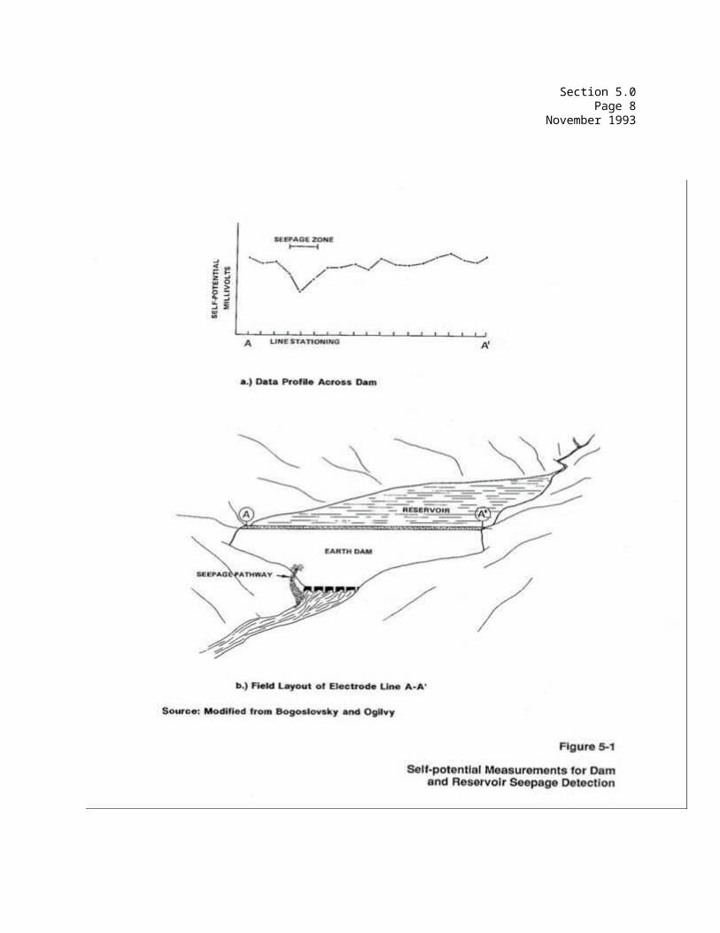
Section 5.0Page 9
November 1993
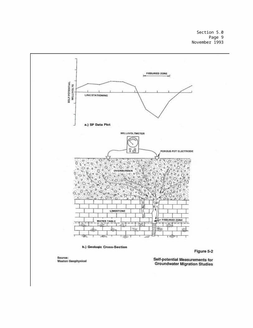
COMMONWEALTH OF MASSACHUSETTS
DEPARTMENT OF ENVIRONMENTAL PROTECTION
STANDARD REFERENCES FOR GEOPHYSICAL INVESTIGATIONS
SECTION 6.0 ELECTROMAGNETIC INDUCTION METHODS (EM)
Section 6.0Page i
November 1993
SECTION 6.0ELECTROMAGNETIC INDUCTION METHOD
TABLE OF CONTENTS
Section Title Page No.
6.1 OVERVIEW......................................... 1
6.1-1 Terrain Conductivity............................. 16.1-2 VLF.............................................. 2
6.2 INTRODUCTION..................................... 3
6.2-1 Terrain Conductivity............................. 36.2-2 VLF.............................................. 6
6.3 APPLICATIONS..................................... 7
6.3-1 Terrain Conductivity............................. 76.3-2 VLF.............................................. 8
6.4 EQUIPMENT........................................ 8
6.4-1 EM (terrain conductivity) Equipment.............. 86.4-2 VLF Equipment.................................... 8
6.5 FIELD PROCEDURES................................. 9
6.5-1 Terrain Conductivity Field Procedures............ 96.5-2 VLF Field Procedures............................. 10
6.6 INTERPRETATION................................... 11
6.6-1 Data Analysis.................................... 11
6.6-1.1 Terrain Conductivity............................. 116.6-1.2 VLF.............................................. 11
6.6-2 Presentation of Results.......................... 12
6.6-2.1 Terrain Conductivity............................. 126.6-2.2 VLF.............................................. 12
6.6-3 Interpretation................................... 12
6.6-3.1 Terrain Conductivity............................. 126.6-3.2 VLF.............................................. 12
Section 6.0Page ii
November 1993
SECTION 6.0ELECTROMAGNETIC INDUCTION METHOD
TABLE OF CONTENTS (continued)
Section Title Page No.
6.7 ADVANTAGES AND LIMITATIONS....................... 13
6.7-1 Terrain Conductivity............................. 136.7-2 VLF.............................................. 14
6.8 GLOSSARY........................................ 15
REFERENCES ................................................. 17
Section 6.0Page iii
November 1993
LIST OF FIGURES
Figure Title Page No.
6-1 Two-coil Electromagnetic Induction Apparatus........................................ 20
6-2 Conductivity Ranges for Common Earth Materials........................................ 21
6-3 Conductivity Contour Map......................... 22
6-4 Typical EM Response Over a Metal Pipe............ 23
6-5 Comparison of Relative Responses for Vertical and Horizontal Dipoles.................. 24
Section 6.0Page 1
November 1993
6.0 ELECTROMAGNETIC INDUCTION METHOD
6.1 OVERVIEW
Electromagnetic Induction (EM) methods are non-destructive geophysical techniques for measuring the apparent conductivity of subsurface materials. As with resistivity surveys (Section 4.0), the general principal of EM surveys is that dissimilar subsurface materials can be identified by the differences in their respective electrical responses to the introduction of an electrical stimulus. There are two basic types of EM surveys, terrain conductivity and Very Long Frequency (VLF). Each survey method is explained below. Terrain conductivity, given its broader applicability and usage in environmental studies, is explained in greater detail.
6.1-1 Terrain Conductivity
Terrain conductivity surveys employ the same operating principals as conventional resistivity surveys (Section 4.0), but differ from resistivity surveys in the manner with which an electrical stimulus is introduced to the earth. The terrain conductivity method of EM surveying is an active geophysical technique that involves "inducing" an electric current in the subsurface and measuring the subsequent electrical response at the ground surface to characterize the physical properties of subsurface materials. In contrast, resistivity surveys directly apply an electrical current to the ground using current electrodes and measure the resultant voltage potential using measurement electrodes. The resistivity method requires that electrodes are driven into the ground and connected with wires at each survey point. Terrain conductivity surveys employ a transmitting coil, which is not directly coupled to the earth, to remotely induce a voltage potential in the ground and a receiving coil to measure a secondary current created by the effect of the induced voltage in a conductive medium.
The name "terrain conductivity" stems from the different manner (with respect to resistivity surveys) with which terrain conductivity measures the electrical properties of the materials investigated. The resistivity method directly applies a current (I) to the ground, measures the resultant voltage (V), and calculates the resistivity (R) of the material measured (given that V=IR). Terrain conductivity surveys use a known current (I), passed through transmitting coil to create an electromagnetic field which induces a voltage (V) in the ground. If the ground material is conductive, then a secondary (induced) electromagnetic field will be created. The terrain conductivity receiving coil measures the currents (I) created by the primary (transmitted) electromagnetic field and the secondary (induced) electromagnetic field. The ratio of these two currents is proportional to the conductivity (which is the inverse of resistivity, R) of the material being surveyed. (A more complete explanation of the inductive measurement theory is presented
Section 6.0Page 2
November 1993
below in the Introduction.)
Terrain conductivity surveys identify geoelectric layers rather than geologic ones. A geoelectric layer is a layer which exhibits a similar electric resistivity response. A geoelectric layer can, but does not always, correspond to a geologic one. For example, an isotropic homogeneous sand, which is saturated with a fluid exhibiting a single conductivity response, will appear to be a single geoelectric layer. The same sand, if filled with fluid layers containing different conductivities, (i.e. salinities) will appear to be more than one geoelectric layer. The interpretation of terrain conductivity data is therefore best made in conjunction with other geophysical techniques (i.e., seismic refraction, Section 3.0) or conventional subsurface investigations (i.e., soil borings).
The terrain conductivity survey method is non intrusive and can be conducted at a more rapid pace (and less expensively) than conventional resistivity surveys. The portable instrument requires only a one or two person field party. Measured conductivity values can be observed during data acquisition, and yield immediate preliminary information for an experienced operator. For this reason, terrain conductivity survey methods have generally supplemented resistivity surveys as the method of choice for shallow horizontal profiling of the subsurface.
Common applications for terrain conductivity surveys include: shallow contaminant plume mapping; locating buried metallic objects; identifying landfill boundaries; and characterization of subsurface lithology changes and/or changes in moisture content. As with other geophysical techniques, the effectiveness of terrain conductivity interpretation is increased by correlation with other geophysical techniques. For example, the combination of terrain conductivity and magnetometry surveys (Section 8.0) is ideal for a combination of location of buried drums while the combined use of terrain conductivity and seismic surveys (Section 3.0) will effectively differentiate between conductive contaminant plumes and landfill boundaries.
6.1-2 VLF
The VLF survey method is an EM prospecting technique based on the principle of radio wave transmission and reception. The VLF method does not employ an operator induced electromagnetic field, but instead utilizes low frequency transmissions from a submarine communications network established and maintained by the U.S. Navy as a power source.
The VLF receiver measures the current density due to the primary (transmitted) and secondary (induced) magnetic fields. From these measurements, structures such as water-saturated fracture zones, metallic ore bodies, mineralized zones, and long conductors such as electric
Section 6.0Page 3
November 1993
cables or pipelines may be detected. The ability to detect water-filled bedrock fracture zones makes this type of survey method useful for bedrock water supply development and for site investigations which involve bedrock contamination.
VLF survey limitations are: susceptibility to surface anthropogenic interferences (e.g., fences, automobiles, power lines). The effective depth of VLF investigation is extremely reduced in areas that contain shallow material of high conductivity.
6.2 INTRODUCTION
6.2-1 Terrain Conductivity
The terrain conductivity method utilizes an internal transmitter/ receiver system to measure the conductivity of earth materials. The principle of terrain conductivity surveying is as follows. When a current (primary current) of varying intensity (either a continuous wave or transient current) is passed through a wire (in the case of EM survey, a coiled wire), a primary magnetic field is created. The magnetic field expands and collapses as the current strength increases and decreases. This expansion and collapse of the magnetic field creates (induces) a voltage (or electromotive force) within the area of the magnetic field, the strength of which is proportional to the rate of the magnetic fields expansion and collapse.
If the primary (transmitted) magnetic field induces a voltage in a conductive medium (in this case, the Earth), then a current flow will be created. The strength of this current is directly proportional to the conductivity of the medium. A secondary magnetic field, which expands and collapses with current flow in the earth, is in turn created. This secondary magnetic field produces a voltage which causes a secondary current to flow in the receiving coil. Electrical conductivity values of subsurface materials are determined by measuring the secondary electromagnetic field produced as illustrated in Figure 6-1. Terrain conductivity instrumentation measures the currents created by both the primary and the secondary electromagnetic fields. The ratio of the primary electromagnetic field to the secondary electromagnetic field is directly proportional to the terrain conductivity, which enables direct, on-site instrument readout of apparent conductivity values.
The depth of investigation for electromagnetic induction methods is primarily a function of the transmitter/receiver coil spacing and the coil orientation. The greatest depth of investigation (approximately 1.5 times the coil spacing) is achieved by orienting the coils vertically (axis of coil windings is parallel to round surface), while a shallower depth of investigation (approximately 75% of coil spacing) is achieved by orienting the coils horizontally.
The induction method induces current flow throughout the volume of the
Section 6.0Page 4
November 1993
earth that is investigated. The secondary current measured by the instrument is therefore a composite of current contribution of the different depth intervals influenced by the transmitting coil. By varying the coil configuration and/or coil spacing, it is possible to determine the conductivity of the various stratigraphic layers within the depth of investigation.
Because terrain conductivity instrumentation induces the current to the earth, it does not suffer from the physical conditions which impede conventional resistivity surveys, such as snow, ice, permafrost, and shallow gravel or bedrock constraints.
It is of interest to note that the inductive method will allow the observer to measure the conductivity of a stratigraphic layer which lies below a thin (e.g., less than two meters thick) zone of infinitely resistive material found at the surface. This would not be possible using the conventional resistivity.
Conductivity ranges typical of various earth materials are shown on Figure 6-2. EM conductivity values are usually expressed in units of millimhos per meter (or millisiemens/meter). Computer software is available for modeling (forward or inverse) either VLF or terrain conductivity data.
As mentioned previously, electrical conductivity measured during an EM survey is a function of the subsurface materials. Specific properties of soil, rock, and groundwater which affect electrical conductivity are:
o Material composition
o Water content (porosity and degree of saturation)
o Salinity or ion content of the water
o Permeability
o Temperature
Material composition plays a large role in the conductivity of a substance and, in the case of rocks and minerals, can vary widely. For example, clay has a conductivity of the order of 10-3 mmho/meter, whereas some dry quartzite rocks have resistivities of more than 10-9 mmho/meter (Cully et al, 1975). No other physical property of naturally occurring rocks or soils displays such a wide range of values. The approximate ranges of conductivity for common soil and rock types are shown in Figure 6-2. The ranges of conductivity values for a single material generally indicate conductivity variations between dry and water-saturated conditions. Dry sands, gravels, and massive unweathered rock typically exhibit relatively low conductivities; clays, clayey tills, water-saturated sediments, and weathered rock (chemically broken down to clays)
Section 6.0Page 5
November 1993
tend to have higher conductivities.
The water content (which is a function of material porosity and the amount of pore saturation) of a material is the greatest single factor controlling the electrical characteristics of subsurface geology. Most soil and rock materials are relatively poor electrical conductors (i.e., exhibit low conductivities) compared with groundwater. An applied electric current is conducted almost entirely by the water in the pore spaces or fractures of soil or rock rather than by the soil or rock alone. This also applies to the unsaturated (vadose) zone, because in general there is some moisture in unsaturated media. Dry material yields lower values of conductivity; accordingly, it is more difficult for electricity to pass through layers such as dry sands or gravels. Conversely, if materials are saturated (especially in the case of clays) electricity can pass through the layering more easily and such layers are referred to as good electrical conductors (low resistivity materials).
Salinity (or ion content) also plays an important role in the resistivity of a material. If salts are present (such as nearby ocean environments or areas adjacent to roadways kept clear of ice by the practice of spreading salt) recorded data will reflect abnormally high conductivity values for the subsurface material. On the other hand, pure (distilled) water is non-conductive, however, most groundwater contains some dissolved salts and hence is somewhat conductive.
Formation permeability (as well as conductivity) is a function of, and is directly proportional to, the interconnectedness of the formation pores. The geometrical arrangement of the pore spaces may make formation resistivity conductivity anisotropic. The vertical resistivity of a geoelectric layer, which would be more likely to effect a surface conductivity measurement, could therefore be different than the horizontal conductivity, which would be determined from a borehole resistivity survey (see Section 10.3-5).
The temperature of a formation will also affect the electrochemical activity of groundwater and will therefore also effect conductivity of the medium. Fluid conductivity is directly proportional to the temperature. In most cases, however, subsurface temperature variation is minimal and therefore conductivity corrections are not necessary.
A basic principal of EM surveys is: the greater the distance between the current and the measurement coils, the greater the depth of investigation. Widely spaced traverses or soundings are used for reconnaissance surveys or for delineation of large targets (horizontally extensive clay or gravel layers). Closely spaced data are required for identification of localized features such as discrete zones of leachate migration, etc.
EM measurements are commonly used to delineate either changes in
Section 6.0Page 6
November 1993
conductivity with depth or lateral variations in resistivity. These applications are known respectively as:
o Vertical electrical soundings (VES)
o Horizontal profiling
VES surveys, which determine vertical conductivity changes, are best conducted with instruments which allow variable coil spacings (e.g., Geonics EM 34). A limited (by depth of investigation) VES survey can also be conducted using a fixed coil spacing instrument (e.g., Geonics EM-31) by altering the orientation (turning on its side) of the measuring equipment. VES surveys are used to identify geoelectrical layering in soil and rock. These data are often used to identify the groundwater table, clay layers, and the bedrock surface.
For horizontal profiling, which determines lateral resistivity changes at a fixed depth of investigation, the current measurement coil spacings are kept constant. A fixed coil spacing instrument can be operated by one person and is well suited for horizontal profiling. Horizontal profiling is used to identify lateral resistivity variations in a survey area. Horizontal profiling can be used to detect conductive groundwater plumes, landfill limits, geologic contacts, and sink holes (often present in limestone lithology).
6.2-2 VLF
The VLF method does not employ an operator induced electromagnetic field, but instead utilizes low frequency transmissions from a submarine communications network established and maintained by the U.S. Navy as a power source.
VLF signals are transmitted by vertical radio antennae several hundred feet high with signal outputs ranging from 300 to 1,000 kWatts. The effective range of these transmitters as a VLF survey power source is on the order of thousands of miles. (It should be noted that a site must be a minimum of 50 miles from a transmitter for this technique to be effective.) A worldwide network of VLF stations has been established in such varied locations as Bordeaux, France (15.1 kHz), Moscow, USSR (17.1 kHz), and Cutler, Maine (24.0 kHz).
The field emitted by VLF antennae is horizontal, and its magnetic lines comprise concentric rings that "ripple" out from the transmitter. When this magnetic field encounters an electrically conductive structure on the surface or underground, weak secondary currents are generated around the structure. These currents create a secondary magnetic field.
VLF can detect long conductors such as electric cable and pipelines. In order for the VLF method to be effective in detecting underground geologic structures, structure must have: 1) the direction of its long
Section 6.0Page 7
November 1993
axis within 30 degrees of the direction of the transmitter (to initiate induction); 2) minimum dimensions of approximately 50 meters in length, 10 meters in depth, and about one meter in thickness; 3) a dip angle not less than 30 degrees from horizontal; and 4) higher electrical conductivity than the surrounding material.
Unlike terrain conductivity, the depth of VLF penetration is not a function of coil spacing, but rather the resistivity of the materials surveyed. Depth of penetration of VLF signals is directly proportional to (varies by approximately four times the square root of) the material's resistivity. For example, VLF signals propagating through granite (a highly resistive material) can penetrate to depths greater than 300 meters. However, a material such as salt water may limit depth of penetration to one to five meters.
6.3 APPLICATIONS
6.3-1 Terrain Conductivity
The measurement of terrain conductivity provides a valuable contribution to environmental site characterization. The applications include:
o Mapping conductive contaminant groundwater plume
o Locating buried abandoned trenches and lagoons
o Delineating bedrock fracture zones
o Determining thickness of weathered bedrock layers
o Mapping lithology
o Locating buried metallic objects
o Locating lateral changes such as pockets or pits of different materials
Examples of applications at sites where groundwater is contaminated are presented by Duran (1982), Greenhouse (1983), and Greenhouse and Slaine (1983).
Contaminant plumes in the saturated zone can be mapped provided there is a sufficient change in the conductivity to be detected by the instrument. Generally, contaminant plumes of inorganic waste are easily detected because the pore fluids often have conductivity values as much as three orders of magnitude above background values. Figure 6-3 illustrates an anomaly representing a contamination plume resulting from landfill leachate.
Section 6.0Page 8
November 1993
Conductivity measurements can also be used to detect the presence of buried waste, filled disposal trenches, and buried metal objects such as drums, tanks or metal debris. Figure 6-4 illustrates an anomaly over a buried metal object.
6.3-2 VLF
The VLF device has the deepest depth of investigation of EM techniques and is generally used to evaluate large geologic structures (such as fault/fracture planes). VLF is also useful for bedrock fracture trace analysis for both environmental site assessments and water supply development.
6.4 EQUIPMENT
6.4-1 Terrain Conductivity Equipment
Terrain conductivity (two-coil) induction instrumentation systems consist of a transmitter coil and a receiver coil (see Figure 6-1). The transmitter coil induces an electromagnetic field of known strength and the receiver coil measures the resulting quadrature (i.e., ratio of secondary to primary fields) resulting from subsurface features. The instrument is read directly in units of millimhos per meter (conductivity). EM readings represent the average bulk conductivity at a point halfway between the two coils.
The sampling depth or depth of investigation is related to the coil spacing and coil mode. The two coil modes used are the vertical and horizontal dipole modes. Figure 6-5 shows the relationship of the coil spacings, mode and relative responses. Either vertical sounding or horizontal profiling can be done. Vertical sounding is accomplished by multiple measurements about a point with varying coil spacing in order to penetrate deeper and discern layering; therefore called a "sounding" method. Horizontal profiling is performed by making measurements along traverses with a fixed coil spacing; therefore detecting lateral variations along designated lines of investigation. General discussions of electromagnetic induction methods are presented in texts by Grant and West (1965), Telford and others (1976), and Griffiths and King (1981).
6.4-2 VLF Equipment
The VLF Instrumentation is a small, lightweight hand-held instrument which can be operated by one person. Principal components of the instrument are a pair of mutually perpendicular coils and a receiving crystal with a frequency tuned specifically to a transmitting antenna. The two receiving coils are used to measure local characteristics of the primary induced field and any secondary fields emanating from bodies of variable conductivity. The instrument is read in units of percentage (which are ratio comparisons of field strengths).
Section 6.0Page 9
November 1993
6.5 FIELD PROCEDURES
6.5-1 Terrain Conductivity Field Procedures
Terrain conductivity conductivity data can be acquired using sounding and profiling techniques similar to those used in electrical resistivity (see Section 4.0 Resistivity Methods). Horizontal profiling is accomplished by traversing an area with a fixed coil spacing and orientation. Terrain conductivity vertical electric sounding (VES) is accomplished by expanding the inter-coil spacings in a manner similar to that used by electrical resistivity soundings.
Important information that should be sought before conducting a terrain conductivity survey are: the assumed hydrogeologic characteristics of the site; potential source locations and migration paths; characteristics of the hazardous substance of interest; and depths of interest. The level of detail necessary (size of object of interest and detail of resolution) determines the number of survey points and station spacings required. The depth of investigation required determines the spacing of the terrain conductivity coils. Terrain conductivity induction instruments may have a depth of investigation of up to 200 feet depending on coil spacing and orientations used (see Figure 6-5).
For a terrain conductivity type of induction survey, a regular pattern of survey stations is usually preferred. Typically, use of a grid spacing which is approximately equal to the size of the target sought by the survey, and a coil spacing with a maximum response for the depth of interest will produce satisfactory results. Specific needs for local detail, however, may require a refined coverage. The chosen spacing should always be site- and target-specific.
The factors that will determine which instrument is used and what the grid spacing should be at particular sites are:
o Depth to target and size of target;
o Accessibility of the site;
o Effects of manmade structures and utilities, such as electric power lines; and
o Conductivity of the earth materials.
In conducting a terrain conductivity survey, the field operator must avoid or note any potential sources of interference such as power lines, buildings, fences, buried pipelines or any other large metal objects.
Section 6.0Page 10
November 1993
Noise sources should be noted on the profiles or contour maps so that anomalies due to these known sources can be accounted for.
Terrain conductivity data, if not recorded on a strip chart or digital recording instrument, should be recorded on standardized data sheets. At a minimum, all data (strip chart, digital disks, or standard forms) should have the following information listed:
o Project/site location identification
o Company
o Date and time
o Operator's name
o Instrument make, model
o Coil spacings and configuration
o Line and station numbers
o Instrument reading scales
o Weather conditions/temperature
6.5-2 VLF Field Procedures
In conducting a VLF survey, VLF readings should be acquired with the instrument oriented perpendicular to a straight line from the site to the transmitter antennas. This orientation ensures optimum data quality. All readings from a particular VLF station must be obtained with the instrument oriented in the same direction.
As with all geophysical surveys, an octagonal survey grid is advised to facilitate accurate location of survey anomalies. For VLF surveys, however, the orientation of the survey grid is almost irrelevant, since the critical parameter for inductive coupling (between the VLF signal and the object of interest) is the relationship between the strike of the conductor and the bearing of the transmitting station (parallel configuration being the optimum).
A body which strikes towards (is parallel to a line drawn between the transmitting station and the site) the transmitter is said to be well-coupled, since the magnetic vector of the VLF electromagnetic field is at right angles to the body and therefore, the induced current can flow freely through it. Otherwise current flow will be restricted, reducing the strength of the secondary field making detection difficult, if not impossible. An attempt should therefore be made (by reviewing bedrock maps and/or bedrock photolineament analyses) to determine the strike of
Section 6.0Page 11
November 1993
bedrock fractures before the start of a field program so that the proper VLF transmitter station can be chosen for the survey.
At the start of a VLF survey, the receiver is tuned to a properly oriented VLF station and data is acquired perpendicular to the strike of the target structure. If the probable strike of the conductors cannot be determined before the start of the VLF survey, two transmitters, bearing roughly at right angles, should be used to conduct a survey across the area of interest. All readings in a survey should be taken with the instrument facing in the same direction. This direction must always be recorded in the field notes. A recommended standard practice, is to specify a standard range of directions (e.g., N and E rather than S or W) for use on all surveys.
Visible structures such as cables, power lines, metal pipes, and electric fences (which would generate their own VLF anomalies) are carefully documented to simplify data interpretation.
6.6 INTERPRETATION
6.6-1 Data Analysis
6.6-1.1 Terrain Conductivity
In general, terrain conductivity survey data require relatively little processing before they can be interpreted. This is especially true for fixed coil spacing (horizontal profile) surveys on-site because the data are directly recorded in units of conductivity. Preliminary interpretations are made by comparisons with other nearby conductivity values. A contour map can be prepared from the data and compared with results of other surveys.
Terrain conductivity data also can be used for vertical electric sounding (VES) analysis similar to resistivity VES. Data acquired during EM VES surveys are easier to work with because the instruments read directly in units of conductivity. EM VES, however, has lower resolution than that performed with the resistivity technique. A VES contour map and/or profiles can be prepared from the data and compared with results of other surveys.
6.6-1.2 VLF
VLF instruments do not read directly in units of conductivity. The in-phase measurement (the tilt of primary induced field is read in terms of the tangent to the angle of tilt) is given as a percentage. Quadrature measurements (which are the ratios of voltage required to equalize the primary to secondary signal strengths) are also given as percentages. For field interpretation these two sets of data can be plotted in profile form, percentage versus distance.
Section 6.0Page 12
November 1993
6.6-2 Presentation of Results
6.6-2.1 Terrain Conductivity
Results of a terrain conductivity survey can be presented in profile and/or contour map form. The orientation of the traverses should be indicated on profiles, and lines of coverage shown on contour maps. Locations of observed surface metal and other cultural features such as topography, buildings, fences, and power lines should be noted on both the profiles and the contour maps.
6.6-2.2 VLF
VLF data are presented as two curves, often referred to as the in-phase and quadrature phase components of the VLF measurement. The strike and dip information derived from VLF data interpretation is easily presented with a profile format.
VLF data can also be presented in contoured format and compared to other available data such as resistivity and magnetics. Digital data acquisition systems are now available that facilitate calculation of conductivity.
6.6-3 Interpretation
6.6-3.1 Terrain Conductivity
Terrain conductivity data can be analyzed qualitatively and quantitatively. Generally, profiling data are presented as contour maps or profiles. Profile lines should be stacked and aligned. A qualitative analysis of the contour map or aligned profiles usually can allow an interpreter to identify any conductivity trends that may be indicative of buried metal, groundwater flow and contaminant transport. A comparison of available geologic data, and cultural, ferrous metal and debris maps prepared during data acquisition, should be made to evaluate the causes of any conductivity trends observed.
Computer or chart comparisons of terrain conductivity sounding data with available theoretical models can be made. This type of interpretation is similar to that used in electrical resistivity, but in terrain conductivity sounding it is limited to relatively simple hydrogeologic conditions.
6.6-3.2 VLF
In order to interpret VLF data, it is important to know the orientation of the object to the VLF transmitter station. Instrument orientation during the survey must also be known to allow accurate data interpretation.
Section 6.0Page 13
November 1993
6.7 ADVANTAGES AND LIMITATIONS
6.7-1 Terrain Conductivity
Advantages
Advantages of the terrain conductivity method include:
o No ground intrusion required - Terrain conductivity is an induction method which does not require repeated contact with the earth across a survey area.
o Rapid data acquisition (faster than resistivity) - Because no physical intrusion at each station is required, data acquisition is much faster. In fact, for horizontal profiling with fixed coil equipment, data can be acquired literally as fast as the operator can walk.
o Lightweight, one- or two-man operation - Equipment is self contained and battery powered. Fixed coil spacing equipment can be operated by one person. Even a small person can easily handle the equipment.
o Wide range of applications - As stated previously in this section, terrain conductivity can be used to: map contaminant plumes, locate buried metal objects, and identify landfill boundaries.
o High lateral resolution - Horizontal profiling surveys can often accurately identify the location of anomalies as small as a single drum.
o Field interpretation possible - The instrument response is directly proportional to subsurface conductivity and, therefore, can be used to quickly identify anomalous areas.
Limitations
Limitations of the terrain conductivity method include:
o Limited dynamic range (1 to 1,000 millimho/meter) - A measurable secondary electromagnetic field cannot be induced in materials with low conductivity (high resistivity). In the case of extremely conductive materials, the instrument response is no longer directly proportional to subsurface conductivity.
o Susceptible to effects of man-made structures, utilities, etc. - Because this technique relies on the induction of an
Section 6.0Page 14
November 1993
EM field, the presence of other EM fields, such as those associated with power lines, causes unwanted interference. Also, since the strength of the secondary field is a function of the conductivity of the material surveyed, the presence of highly conductive objects, such as metal fences, also creates unwanted interferences.
o Less vertical resolution than resistivity - Currently terrain conductivity equipment cannot offer the infinitely variable spacing possibilities that resistivity surveys can. For this reason, resistivity offers superior vertical resolution.
o Limited penetration - Currently terrain conductivity equipment cannot offer the infinitely variable measurement spacing possibilities that conventional resistivity does. The limited strength of the terrain conductivity transmitter signal, due to battery and coil size constraints (a compromise to portability), limits the depth of instrument penetration. For this reason, resistivity offers superior vertical penetration.
o Even simple stratigraphic layering cannot be distinguished without complex application and interpretation - Because the measured signal is a composite of all the subsurface volume affected by the transmitted electromagnetic field. The presence and effect of multiple stratigraphic layers cannot be determined without data analysis.
6.7-2 VLF
Advantages
o Rapid survey technique - As with other EM methods, the non-intrusive data acquisition is rapid.
o Excellent depth of penetration - Under optimum conditions VLF has the greatest depth of penetration of the EM methods.
o Determine the strike and dip of water bearing fracture - This information is very useful in the optimum placement of bedrock wells (which are usually more time consuming and expensive to install than overburden wells) for either site assessment or water supply development projects.
Disadvantages
o No control over power source - VLF transmitters are sometimes turned off for maintenance. Even when the transmitters are operating, the orientation (both strike and dip) of the
Section 6.0Page 15
November 1993
object surveyed to the power source (which the operator also has no control over) will affect the success of the survey.
o Depth of investigation affected by conductivity of material - The more conductive the subsurface is the shallower the depth of investigation is.
o Susceptible to effects of man-made structures, utilities, etc. - Because this technique relies on the induction of an EM field, the presence of other EM fields, such as those associated with power lines, causes unwanted interference. Also, since the strength of the secondary field is a function of the conductivity of the material surveyed, the presence of highly conductive objects, such as metal fences, also creates unwanted interferences.
o Interpretation is difficult - VLF data does not provide data which can be directly related to subsurface conductivity. Interpretation is more subjective and therefore relies heavily on operator experience.
o Limited application - Since conductive objects need to be of a fairly large size (long axis on the order of 50 meters or more) before they can be discerned by VLF method, applicability of this method to detecting anomalies of concern at hazardous waste assessments (e.g., drums and USTs) is limited.
6.8 GLOSSARY
Apparent conductivity - A measured conductivity value that is only indicative of the true value.
Bulk conductivity - Conductivity of a mass of material that may contain metallics and is possibly layered; it is an averaged value for relatively large segments of subsurface materials.
Conductivity - (inverse of resistivity) - Ability of a material to conduct electricity.
Dip - The angle between a horizontal plane and a planar feature of a structure, measured, perpendicular to strike.
Dipole - The two-coil instrumentation system (EM).
Induction method - Electric currents are induced in the earth by a time-varying magnetic field.
Horizontal dipole mode - Transmitter and receiver coils oriented vertically.
Section 6.0Page 16
November 1993
Horizontal profiling - EM measurements along a traverse with a fixed coil spacing and coil orientation.
Strike - The long axis of a structural surface (i.e., bedding or fault plane) as defined by the intersection of the structures with a horizontal plane.
Vertical dipole mode - Transmitter and receiver coils oriented horizontally.
Vertical sounding - Multiple EM measurements centered at a point with varying coil spacings.
Section 6.0Page 17
November 1993
REFERENCES
Culley, R.W., Jagodits, F.L., and Middleton, R.S., 1975, E-Phase system for detection of buried granular deposits: Symposium on modern innovations in subsurface exploration, 54th Annual Meeting of Transportation Research Board.
Duran, P.B., and Haeni, F.P., 1982, The use of electromagnetic conductivity techniques in the delineation of groundwater contamination plumes in Novitzki, R.P. and Levine, G., eds., The impact of waste storage and disposal on groundwater resources, Northeast Conference presented by U.S. Geological Survey and Cornell University Center for Environmental Research, June 18 - July 1, 1982, Ithaca, New York, p. 8.4.1 to 8.4.33.
Geonics Ltd., 1979, EM 31 Operating manual: Mississauga, Ontario, Canada, 58 p, EM 16 VLF Electromagnetic Unit, Operating instructions: Mississauga, Ontario, Canada.
Grant, F.S., and West, G.G., 1965, Interpretation theory in applied geophysics: New York, NY, McGraw-Hill, 583 p.
Greenhouse, J.P., 1983, Surface geophysics in contaminant hydrogeology:in Field methods in contaminant hydrogeology, Proceedings of a hydrogeology field school sponsored by The Groundwater Research Institute, University of Waterloo, April 18-22, 1983, Canadian Forces Base, Borden, Ontario, Canada, 53 p. , and Slaine, D.D., 1983, The use of reconnaissance electromagnetic methods to map contaminant migration: Groundwater Monitoring Review, v. 3, no. 2, p. 47-59.
Griffiths, D.H., and King, R.F., 1981, Applied geophysics for geologists and engineers, 2nd ed.: Elmsford, New York, Pergamon Press, 230 p.
McNeill, J.D., 1980, Electromagnetic terrain conductivity measurement at low induction numbers: Geonics Ltd., Technical note TN-6, Figure 6, p. 7.
Milsom, John, 1989, Field Geophysics: Milton Keynes, England, Open University Press, p. 123-135.
Telford, W.M., Geldart, L.P., Sheriff, R.E. and Keys, D.A., 1976, Applied geophysics: London, England, Cambridge University Press, 860 p.
Zohdy, A.A.R., Eaton, G.P., and Mabey, D.R., 1974, Application of surface geophysics to groundwater investigations: U.S. Geological Survey, Techniques of Water-Resources Investigations, Book 2, Chapter D1, 116 p.
SECTION 6.0
Section 6.0Page 18
November 1993
ELECTROMAGNETIC INDUCTION METHOD
LIST OF FIGURES
Figure Title Page No.
6-1 Two-coil Electromagnetic Induction Apparatus..... 20
6-2 Conductivity Ranges for Common Earth Materials... 21
6-3 Conductivity Contour Map......................... 22
6-4 Typical EM Response Over a Metal Pipe............ 23
6-5 Comparison of Relative Responses for Vertical and Horizontal Dipoles.................. 24
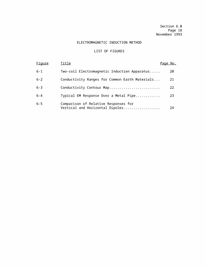
Section 6.0Page 19
November 1993
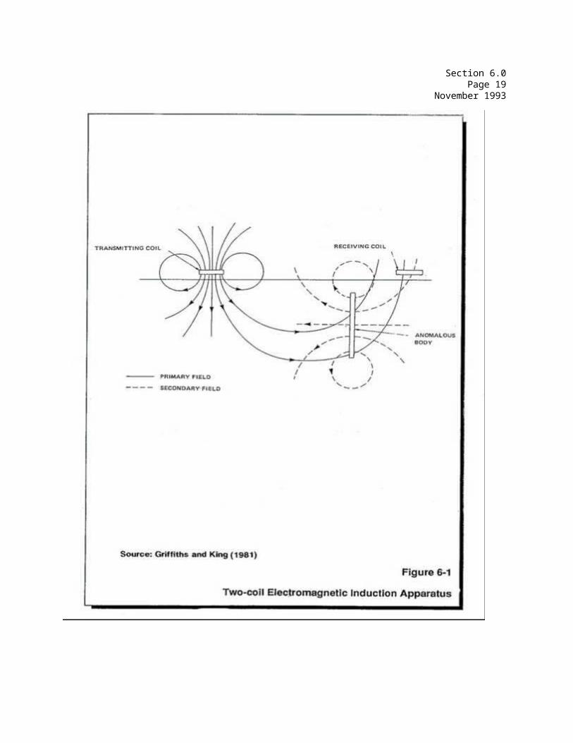
Section 6.0Page 20
November 1993
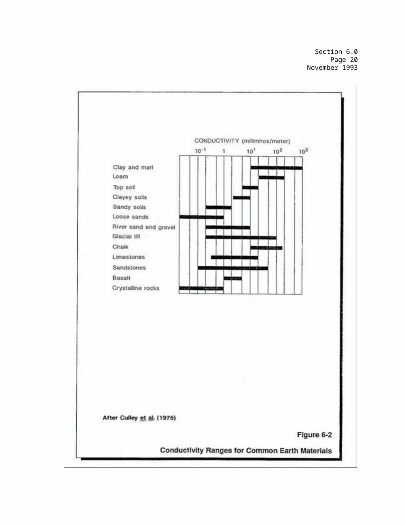
Section 6.0Page 21
November 1993
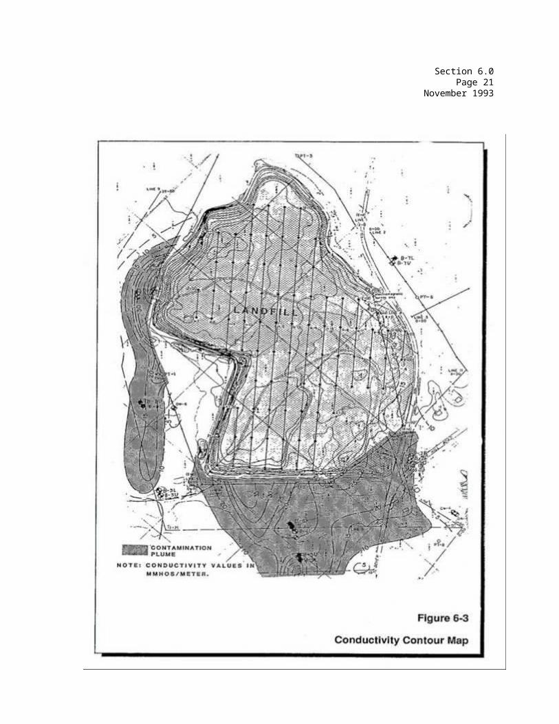
Section 6.0Page 22
November 1993
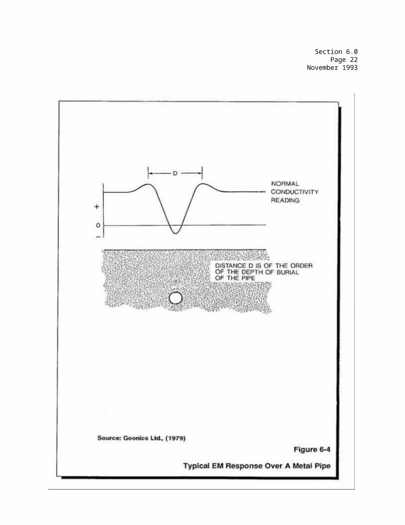
Section 6.0Page 23
November 1993
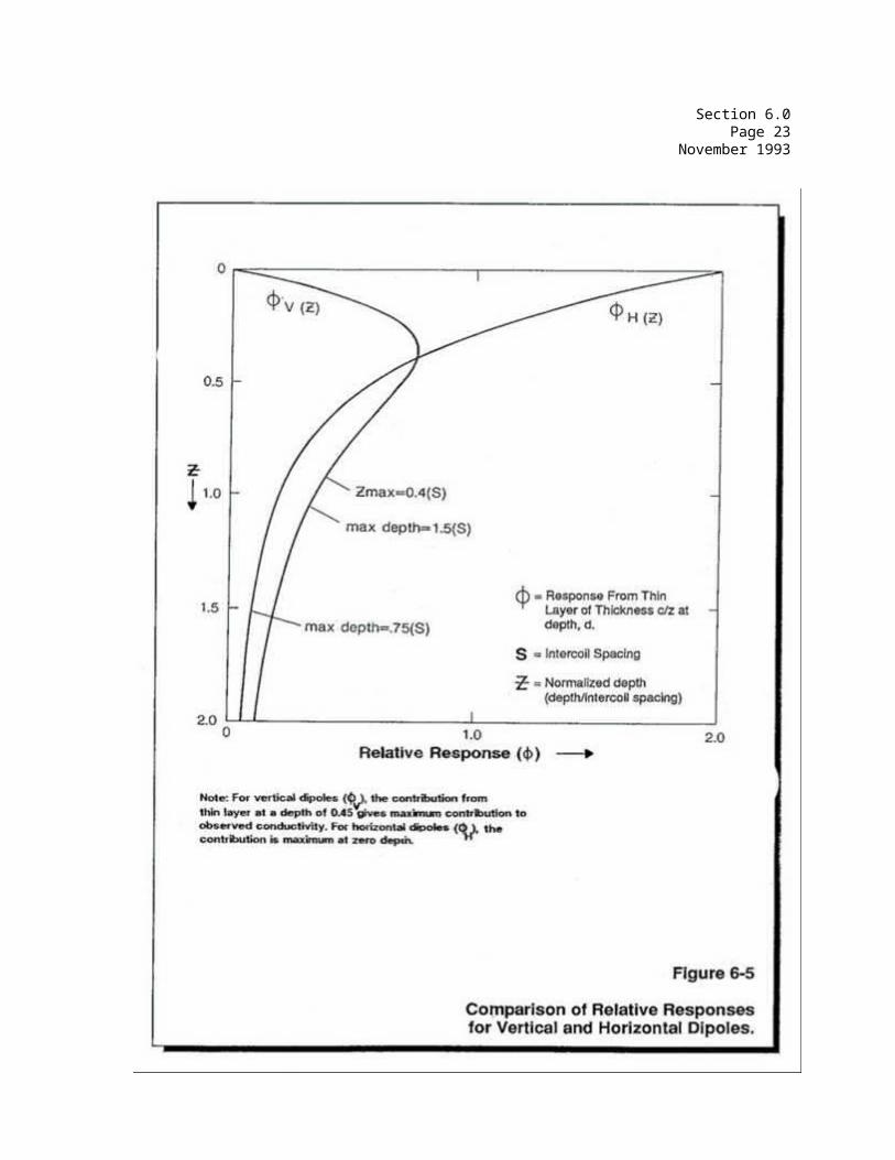
COMMONWEALTH OF MASSACHUSETTS
DEPARTMENT OF ENVIRONMENTAL PROTECTION
STANDARD REFERENCES FOR GEOPHYSICAL INVESTIGATIONS
SECTION 7.0 GROUND PENETRATING RADAR (GPR)
Section 7.0Page i
November 1993
SECTION 7.0GROUND PENETRATING RADAR (GPR)
TABLE OF CONTENTS
Section Title Page No.
7.1 OVERVIEW......................................... 1
7.2 INTRODUCTION..................................... 1
7.3 APPLICATIONS..................................... 3
7.4 EQUIPMENT........................................ 4
7.5 FIELD PROCEDURES................................. 5
7.6 INTERPRETATION................................... 6
7.6-1 Data Analysis.................................... 67.6-2 Presentation of Results.......................... 67.6-3 Interpretation................................... 7
7.7 ADVANTAGES AND LIMITATIONS....................... 7
7.8 GLOSSARY......................................... 9
REFERENCES ................................................. 10
Section 7.0Page ii
November 1993
SECTION 7.0GROUND PENETRATING RADAR (GPR)
LIST OF FIGURES
Figure Title Page No.
7-1 Ground Penetrating Radar Set-Up.................. 13
(a) Radar System Block Diagram.................. 13(b) Typical Radar Record........................ 13
7-2 Ground Penetrating Radar Record of a Buried River Channel............................. 14
7-3 Ground Penetrating Radar Record of Buried Fuel Tanks....................................... 15

Section 7.0Page 1
November 1993
7.0 GROUND PENETRATING RADAR (GPR)
7.1 OVERVIEW
Ground penetrating radar (GPR) is an active geophysical system which transmits high frequency (80-1,000 MHz) electromagnetic waves (radar energy) into the ground and records the energy reflected back to the surface. It is a reflection technique similar to the single-trace seismic reflection method commonly used in marine subbottom profiling (Section 11.2-1). The two techniques differ in that the seismic method uses audio frequency sound waves, while the radar method uses electromagnetic waves. GPR is a continuous profiling method that transmits radar energy into the ground and records the radar energy reflected back by subsurface objects or layers. GPR is useful when a rapid survey with detailed vertical and horizontal control is desired. A GPR survey produces a graphic cross-sectional view of earth stratigraphy and targets (i.e., drums, pipelines, utilities, boulders, etc.) below the ground surface. Under optimum conditions, this method can be effective to depths of 70 feet (using commercially available equipment), although depth penetration is more often limited to the range of ten feet or less below ground surface.
GPR has been used to locate: underground storage tanks; underground pipes; buried drums; buried foundations; voids in rock and concrete; buried archaeological artifacts, excavations, filled pits and lagoons, and numerous other site specific applications and lithologic contacts. GPR can also be used to determine: stratigraphy; depth to the water table; and depth to bedrock. Additionally, GPR has been succssfully used to delineate the lateral extent of conductive contaminant plumes.
7.2 INTRODUCTION
In a GPR system, high-frequency impulses of electromagnetic energy are generated by a transmitting antenna located in a housing which is pulled over the ground surface. Each impulse propagates downward through the ground surface and into the material below. After transmitting the outgoing pulse, the antenna instantly switches from a transmitting mode to a receiving mode in order to detect the reflected signals. Electromagnetic signals are reflected back to the surface from the points of contact (interfaces) of materials with differing electrical properties, such as dielectric permittivity and conductivity. At these interfaces, part of the signal is reflected back to the surface while the remaining signal energy propagates still deeper to be reflected by other layers or isolated bodies. The greater the contrast in the dielectric permittivity (dielectric constant) between two materials, the more energy is reflected
Section 7.0Page 2
November 1993
to the surface. Reflections typically occur at lithologic changes, subsurface discontinuities, and internal soil/rock structures, such as:
o top of bedrock surface
o soil and rock stratification
o water table
o buried metal objects such as drums and utilities
o open and water-filled voids
o bedrock fractures
o archaeological structures and artifacts
o conductive seepage and leachate zones
Signal penetration is also dependent on the frequency of the transmitting antenna used in the radar system. Radar systems are designed to use antennas of various electromagnetic transmission frequencies (80, 120, 250, 300, 400, 500, 900, and 1,000 MHz antennas are commercially available). Selection of the antenna frequency is dictated by the requirements of the survey. The higher frequency antennas which produce waves with shorter wave lengths give better resolution than longer frequency energy sources, but are attenuated more rapidly with depth. If high resolution, near-surface data is desired, a small, high frequency antenna is used. The 900 and 1,000 MHz antennas are used almost exclusively for short penetration capabilities such as for detection of rebar in concrete, where penetration is generally limited to 2 to 3 feet. If project requirements dictate deeper probing (i.e., tens of feet), a larger, lower frequency antenna is used. Specially designed 2 MHz antennas have been used to detect the ice-rock boundary beneath a 2 km thick glacier. Using lower frequency antennas sacrifices resolution of smaller targets for increased penetration. Low frequency antennas (less than 250 MHz) are generally not shielded, making them susceptible to overhead powerline noise and other undesired interference reflections (i.e., passing cars).
The depth of GPR signal penetration is site-specific, being limited by the reflection or the attenuation of the electromagnetic energy. In a layered medium a single, highly reflective (to radar energy) layer (e.g., dry salt) alone can limit signal penetration by preventing the propagation of energy through it. In this instance the apparent loss of energy is caused by reflection rather than by signal attenuation. Signal attenuation is a
function of the characteristics of the subsurface materials being surveyed and is controlled by the four mechanisms listed below:
Section 7.0Page 3
November 1993
o scattering losses
o conduction losses
o water losses
o clay losses
"Scattering losses" are energy losses which occur when the radar signals are dispersed in random directions, away from the receiving antenna, by large irregularly shaped objects, such as boulders and tree stumps.
"Conduction losses" are energy losses which are a function of the electrical conductivity of the material being surveyed. Material conductivity varies with mineral composition, the percent of water saturation of the material pore space, and total dissolved solids (salt, heavy metals) within the pore water. The greater the electrical conductivity values of materials at a site, the more signal attenuation (less penetration) there will be. The signal penetration in sea water, which is highly conductive, is less than a foot.
"Water losses" are energy losses which occur when water molecules are polarized in the presence of the applied electromagnetic field. The radar signals are "lost" when they are converted to kinetic and thermal energy (which cannot be detected by the radar receiver) as a result of the rotation of water molecules.
"Clay losses" occur when electrochemically charged ions along clay surfaces polarize in the presence of the electromagnetic field induced by the radar system. As a result of the polarization, the electromagnetic energy is converted to kinetic and thermal energy and is lost to the radar system. The amount of signal attenuation is directly proportional to the clay content of materials at the site. Olhoeft (1986a) determined that even 5% clay added to a clean sand and gravel will cause a decrease in penetration by a factor of 20.
7.3 APPLICATIONS
GPR can be used for both reconnaissance data gathering and contaminant source detection studies. Typical applications include locating: underground storage tanks; underground pipes; buried drums; buried foundations; voids in rock and concrete; and lithologic contact. GPR can be used to determine: stratigraphy; depth to water tables; depth to bedrock; location of buried archaeological artifacts, excavations, filled pits and lagoons; and numerous other site specific applications. GPR has also been used to delineate the lateral extent of conductive contaminant plumes (e.g., landfill leachate).
As with other geophysical techniques, the cross correlation of GPR data

Section 7.0Page 4
November 1993
with other site data sources (i.e., seismic refraction data, test pits) can facilitate the determination of actual site conditions. GPR results have been correlated with: seismic refraction, to correlate calculated depths of stratigraphic horizons and water tables with radar reflections; magnetometry and electromagnetic induction methods, to verify the presence and locations of buried drums and fuel tanks; and electromagnetic induction and electrical resistivity, to verify the lateral extent of conductive plumes.
7.4 EQUIPMENT
A ground penetrating radar system, shown on Figure 7-1, consists of:
o AC/DC power supply
o coaxial cable(s) which connect the control unit to the antenna
o antenna(s)
o control unit (pulse transmitter)
o graphic recorder
o magnetic tape recorder (optional)
o digital recorder (optional)
Typically, radar antennas contain both the transmitter and receiver within the same fiberglass unit. When a radar impulse is transmitted, the antenna switches to the receiver mode and records reflected radar impulses. The pulse receiver contains an amplifier which increases the amplitude of reflected signals. Bistatic antennas allow the coverage of larger areas with one pass, and multi-receiver combinations allow the "stacking" of radar data which increases the signal-to-noise ratio. Field data are generally printed by a graphic recorder and simultaneously can be stored on magnetic tape or diskette. The graphic recorder produces a continuous time (vertical) versus distance (horizontal) profile of the subsurface for field quality control and qualitative interpretations. Radar impulses are synchronized with the swept-stylus type graphic recorder, producing a dark band proportional to the amplitude of reflected radar signal. Because the antenna is moving, each pass of the stylus represents a slightly different antenna position. Gradually, as the recorder paper advances under the moving stylus, a pattern of reflective interfaces emerges.
The most recently developed GPR field instruments employ digital recording systems that allow on-site data review and color display. The
Section 7.0Page 5
November 1993
colors and tones of collected data can be adjusted to enhance target detection and abrupt changes in layering caused by trenches or pits where dumping or filling has taken place.
Storage of data on diskette or magnetic tape provides an opportunity for additional printing and/or computer processing for the refinement of data. Processing of digital data can enhance stratigraphic reflections from the water table and soil structures (Olhoeft, 1988), and allow easier resolution of metallic targets such as buried drums and the delineation of excavations and sinkholes (Hogan, 1988).
7.5 FIELD PROCEDURES
A sufficient amount of time should be spent to establish recoverable, stationed survey lines in the area of investigation so that detected GPR anomalies can be easily located. In addition, it may be necessary to determine the relative elevation of various points along a traverse so that continuous features may be mapped and presented in terms of elevation rather than depth (e.g., a flat water table surface). Survey lines should be set to maximize coverage, while maintaining a grid spacing proportional to the presumed target dimensions. A maximum survey line spacing of 5 or 10 feet is desired when looking for a small underground storage tank, while a larger spacing of 50 feet or more may be appropriate to define the lateral extent of a conductive groundwater plume.
At the onset of any GPR survey the radar control unit should be adjusted to facilitate the collection of the required data. These adjustments are made by estimating the velocity of the medium and desired depth of penetration. For example, if a radar velocity in soil of 0.4 times the speed of light is assumed, and the objective target is buried 10 feet below ground surface, a minimum time window of 50 nanoseconds is needed. Accurate determination of object depth requires calibration of the radar system. One method of calibrating the GPR system to specific settings is by burying a plate at a measured depth, and moving the antenna slowly along the survey line. The plate will be evident on the GPR record as a thick, dark band, parabolic or flat in shape, with many multiple reflections beneath it. Sakayama and others (1988) describe another method to calculate velocity from bistatic antennas where the receiving antenna is continually moved away from the stationary transmitting antenna. The velocities of the direct arrival and the first strong reflector are re-calculated from the inverse slope of the time-distance display (antenna separation) on the GPR record in a similar manner as seismic refraction.
When a confidence level is attained from depth calibration, the survey is conducted by slowly pulling the antenna along survey lines. A slow walking pace (1-3 miles per hour) increases the horizontal resolution as radar signals are propagated in a 15 to 45 degree cone from the bottom of
Section 7.0Page 6
November 1993
the antenna. A slow walking pace is recommended for hazardous waste investigations as targets are better defined and easier to interpret. On the other hand, the radar antenna can sometimes be towed from the back of a car or truck at speeds up to 10 miles an hour if the "target" is a continuous reflector, such as the water table.
7.6 INTERPRETATION
7.6-1 Data Analysis
A representation of a single GPR signal pulse is shown along the side of Figure 7-1. The horizontal scale of the record is maintained by marking on the record the locations of survey stations as they are reached by the antenna (this is accomplished without interruption of the survey). Typical GPR records produced on the graphics recorder are also shown on Figures 7-2 and 7-3.
Accurate determination of the vertical scale (i.e., conversion of a signal pulse time measurement to a corresponding depth) requires calibration of the radar system, as discussed in Section 7.5. If the depth to a known reflector can not be determined through calibration or verification using boreholes and test pits, the depth to the object can be approximated from relationships involving the velocity of the radar energy through the medium, and the dielectric constant (real dielectric permittivity) of the medium. Values of the dielectric constant for common earth materials can be found in GSSI (1974), and Kutrubes (1986). Depths to reflectors can be calculated using the actual GPR signal travel time measurements and the material velocity value approximated from the dielectric constant value. The validity of this travel time-calculated GPR velocity relationship decreases, however, as soil conductivity increases. The data interpreter should therefore be aware of soil conditions before performing this type of depth calculation.
7.6-2 Presentation of Results
A GPR survey is presented as a graphic cross-sectional view of earth stratigraphy and point targets (i.e., drums pipelines, utilities, boulders, etc.) below the ground surface. Radar impulses are transmitted in sync with a swept-stylus type graphic recorder. The graphic recorder stylus sweeps across the paper at a uniform speed and reflected signals above a user-selected threshold cause the paper to be darkened at points proportional to the amplitude of the reflection. Because the antenna is being pulled forward slowly, each pass of the stylus represents a slightly different antenna position. As the recorder paper advances, a continuous cross-section of reflections from subsurface stratigraphy and point targets is generated.
Digital data stored on magnetic or diskettes tapes can be enhanced using computer processing methods to remove some noise problems, such as
Section 7.0Page 7
November 1993
ringing, or to enhance geologic contact features and point target boundaries. Such methods are described in detail by Hogan (1988) and Olhoeft (1988). Computer processing is typically time consuming and therefore costly and may not be necessary in many instances. The results can therefore be presented as hard-copy, continuous playback with annotations, or in a more limited manner by selectively showing short segments of recordings that illustrate the objectives that were accomplished.
7.6-3 Interpretation
Interpretation of GPR data can be subjective, even among experienced interpreters. For example, a strong and continuous reflected signal across the GPR record may define the boundary between two different types of material (i.e., stratigraphic contact), however, the boundary between the saturated and unsaturated portions (i.e., water table) of the same material may also produce a similar signature on the GPR record.
Point targets, such as buried drums, pipes, boulders, and tree stumps, create a distinctive parabolic feature on GPR records. Positive identification of point targets is subjective, as the GPR signature of a pipe is similar to that of a large boulder, differing only by intensity of the reflection in some cases. Figure 7-3 shows the characteristic parabolic signal created by a buried target, a pipe in this instance, which is situated in a clean sand and gravel deposit. Other metallic objects, such as buried drums, also produce a characteristic parabolic signal on the record, and sometimes produce a "ringing" type of signals denoted by the heavy, dark banding, as shown in Figure 7-3.
7.7 ADVANTAGES AND LIMITATIONS
Advantages
Key advantages of ground penetrating radar surveys include:
o rapid coverage of an area
o a non-destructive non-invasive technique
o portable equipment
o high vertical resolution profiles available in the field for immediate interpretation
Ground penetrating radar provides a cost-effective way of evaluating a large site in a short amount of time. A GPR survey can cover a much larger area of investigation in one day than can be surveyed by seismic refraction or electrical resistivity. The GPR method is "non-destructive" in that it does not require any excavation or probing of the
Section 7.0Page 8
November 1993
overburden materials, although verification of anomalies may be required.
GPR equipment can be easily loaded in the back of a van or carried into inaccessible areas since most pieces comprising the radar system weigh under 40 pounds. Low frequency antennas can be somewhat large and cumbersome; for example, the 80 MHz antenna weighs about 100 pounds and is approximately 4 feet wide.
Since the GPR field equipment includes a graphic recorder, profiled data is observed while operations are underway. This capability is particularly advantageous for detection and the on-site delineation of buried drilling obstructions such as pipes and/or tanks. The capability of real time data analysis and data evaluation can provide savings in overall project time and cost.
Limitations
Limitations of GPR include:
o depth of penetration is usually more shallow than other geophysical methods
o survey lines must be cleared to ground level (e.g., may
require cutting of brush and/or removal of obstructions)
o the depth of signal penetration is highly dependent on the materials present beneath the survey area
o interpretations are subjective, often requiring data corroboration using other geophysical methods and/or verification with borings or test pits
To maximize resolution and minimize scattering losses, survey lines must be as smooth as possible to prevent bouncing and jarring the radar antenna. Survey lines cleared of debris also allow the antenna to be pulled at an even, continuous pace, permitting the easy determination of horizontal scale.
The depth of GPR investigation at a site is limited by soil type and/or the presence of high "loss" materials. Penetration of up to 75 feet has been reported for water-saturated, clean sands in a Massachusetts glacial delta using a commercial antenna. Signal penetration in saturated clays, on the other hand, is on the order of magnitude of only a few inches. In New England, the presence of glacial tills, and lacustrine and marine clays limit the depth of penetration. Delineation of materials beneath a conductive layer may also not be possible.
7.8 GLOSSARY
Section 7.0Page 9
November 1993
Bistatic antenna - An antenna system in which the transmitting and receiver coils are housed in separate antenna units.
Dielectric permittivity (also known as the dielectric constant) - 1. A complex number consisting of a real and imaginary part, which uniquely describes the propagation and attenuation of electromagnetic energy in every material. The real dielectric permittivity (dielectric constant) characterizes the propagation and reflection of EM waves, while the imaginary part (dielectric loss) characterizes the attenuation of EM signal (Kutrubes and Olhoeft, 1987). 2. A measure of the capacity of a material to store charge when an electric field is applied (Sheriff, 1973).
Electromagnetic waves - One of the waves that are propagated by simultaneous periodic variations of electric and magnetic field intensity and that include radio waves, infrared, visible light, ultraviolet, X-rays and gamma rays (Webster's New Collegiate Dictionary, 1979).
Section 7.0Page 10
November 1993
REFERENCES
Benson, R.C., and Glaccum, R.A., 1979, Remote assessment of pollutants in soil and groundwater: in the Proceedings of the 1979 conference on hazardous material risk assessment, disposal and management, Information Transfer, Inc., Miami Beach, April 25-27, p. 188-194.
Geophysical Survey Systems, Inc., 1974, Continuous subsurface profiling by impulse radar: Hudson, NH, pp. 213-232.
Haeni, F.P., McKeegan, D.K., and Capron, D.R., 1987, Ground penetrating radar study of the thickness and extent of sediments beneath
Silver Lake, Berlin and Meriden, Connecticut: U.S.G.S. Water-Resources Investigations Report 85-4108, 19 p.
Hogan, G., 1988, Migration of GPR data: a technique for locating subsurface targets: in Proceedings of the Second International Symposium on Geotechnical Applications of Ground Penetrating Radar, West Gainesville, Florida, March 6-10, 1988, sponsored by the U.S. Dept. of Agriculture, Washington, DC, p. 164-179.
IEEE Wave Propagation Standards Committee, 1977, IEEE Standard definitions of terms for radio wave propagation: IEEE Standard No. 277, Piscataway, NJ, IEEE, Inc., 14 p.
Kutrubes, D.L., 1986, Dielectric permittivity measurements of soils saturated with hazardous fluids: Golden, CO, M.Sc. Thesis, Colorado School of Mines, 300 p.
Kutrubes, D.L., and Olhoeft, G.R., 1987, Dielectric permittivity measurements; applications to GPR: presented at the AGU Fall meeting, December 7-12, 1987, American Geophysical Union Transactions, v. 68, no. 44, p. 1282-1283.
Olhoeft, G.R., 1986(a), Electrical properties from 101 to 109 Hz - physics and chemistry: in Proceedings of the Second International Symposium on the Physics and Chemistry of Porous Media, Houston, TX, Schlumberger-Doll, October, 18 p.
____, 1986(b), Direct detection of hydrocarbon and organic chemicals with ground penetrating radar and complex resistivity: in Proceedings of the Conference on Petroleum Hydrocarbons and Organic Chemicals in Groundwater - Prevention, Detection and Restoration, held Nov. 12-14, Houston, National Water Well Association, Worthington, OH, 22 p.
____, 1988, Applications and limitations of computer-processed ground penetrating radar data: in Abstracts for the Second International Symposium on Geotechnical Applications of Ground Penetrating Radar, West
Section 7.0Page 11
November 1993
Gainesville, Florida, March 6-10, sponsored by the U.S. Dept. of Agriculture, Washington, DC, p. 37.
Sakayama, T., Osada, M., and Tamura, K., 1988, Some examples of archaeological investigations using ground probing radar: in Proceedings of the Second International Symposium on geotechnical applications of ground penetrating radar, West Gainesville, Florida, March 6-10, 1988 sponsored by U.S. Dept. of Agriculture, Washington, DC, p. 57-61.
Sheriff, R.E., 1973, Encyclopedic dictionary of exploration geophysics:Tulsa, OK, Society of Exploration Geophysicists, 266 p.
Section 7.0Page 12
November 1993
SECTION 7.0GROUND PENETRATING RADAR (GPR)
LIST OF FIGURES
Figure Title Page No.
7-1 Ground Penetrating Radar Set-Up.................. 13
(a) Radar System Block Diagram.................. 13(b) Typical Radar Record........................ 13
7-2 Ground Penetrating Radar Record of a Buried River Channel............................. 14
7-3 Ground Penetrating Radar Record of Buried Fuel Tanks....................................... 15
Section 7.0Page 13
November 1993
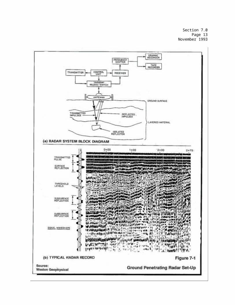
Section 7.0Page 14
November 1993
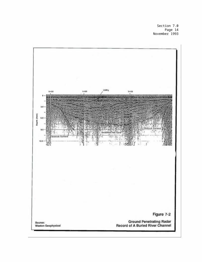
Section 7.0Page 15
November 1993
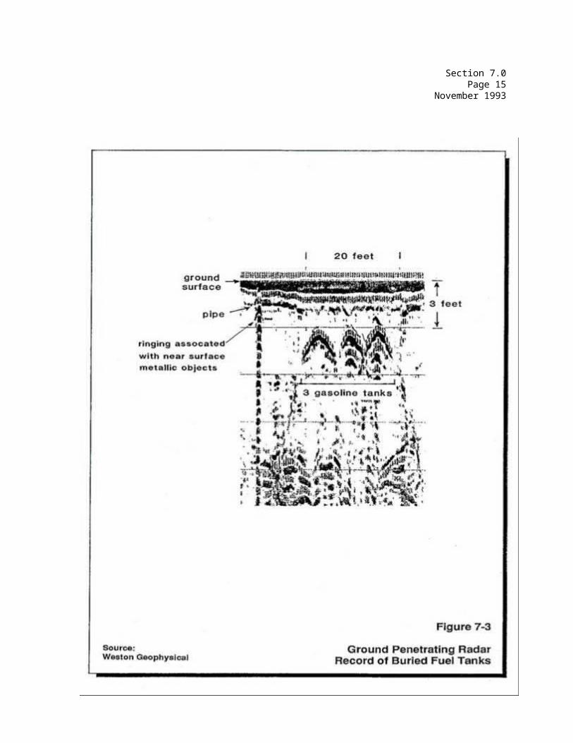
COMMONWEALTH OF MASSACHUSETTS
DEPARTMENT OF ENVIRONMENTAL PROTECTION
STANDARD REFERENCES FOR GEOPHYSICAL INVESTIGATIONS
SECTION 8.0 MAGNETIC METHODS
Section 8.0Page i
November 1993
SECTION 8.0MAGNETICS METHODS
TABLE OF CONTENTS
Section Title Page No.
8.1 OVERVIEW.......................................... 1
8.2 INTRODUCTION...................................... 1
8.3 APPLICATION AND USES............................... 3
8.4 EQUIPMENT......................................... 3
8.4-1 Total Field Proton Precession Magnetometer......... 38.4-2 Vertical Magnetic Gradiometers..................... 48.4-3 Fluxgate Magnetometers............................. 4
8.5 FIELD PROCEDURES.................................. 4
8.6 DATA PROCESSING AND INTERPRETATION................. 5
8.6-1 Data Analysis..................................... 58.6-2 Presentation of Results............................ 68.6-3 Interpretation.................................... 6
8.7 ADVANTAGES AND LIMITATIONS ........................ 6
8.8 GLOSSARY......................................... 7
REFERENCES ................................................ 9
LIST OF FIGURES
Figure Title Page No.
8-1 Magnetic Anomaly from a Buried Barrel............ 11
8-2 Magnetic Anomaly Caused by 75 Barrels Buried 4 to 10 Feet Deep......................... 12
Section 8.0Page 1
November 1993
8.0 MAGNETIC METHODS
8.1 OVERVIEW
Magnetic surveying is a passive geophysical technique which measures the strength of the total magnetic field at any given point on the earth. The purpose of the magnetic survey in environmental investigations is to detect magnetic anomalies (variations in the expected field) which can be attributed to the presence of buried iron or steel objects.
Magnetic surveys, performed as part of environmental investigations, are nearly always used to detect induced magnetism in iron and steel objects such as buried drums, underground storage tanks (USTs), and ferrous landfill refuse. These materials are unique for their ferromagnetic characteristics or ability to be "magnetized".
The results of magnetic surveying can be used to direct excavation activities of buried drums and USTs. The results can be used to direct the placement of both upgradient and downgradient monitoring wells (in conjunction with data regarding the known or inferred direction of groundwater flow) to facilitate the assessment of potential releases of contaminants from these objects on water quality.
Magnetic surveys also have been used successfully to delineate bedrock fracture zones as a result of the weathering of hematite to limonite in certain fracture zones.
An instrument called a magnetometer is used in the performance of magnetic surveys. The magnetometer is used to determine the direction, gradient, and intensity of the total magnetic field. Various forms of magnetometers are used in land, airborne and marine type operations. The land instruments are lightweight and portable, and measurements are readily accomplished by a one or two person field party.Magnetic surveys utilizing portable field magnetometers are relatively easy to perform and are usually the easiest to interpret with regard to siting drilling locations. Magnetic surveys, however, are susceptible to interferences from manmade structures such as utilities, buildings, and fences.
8.2 INTRODUCTION
The earth's magnetic field is believed to be the result of a self exciting dynamo (electrical generator) which is created by the earth's molten metal core spinning as a result of the earth's rotation. A resultant magnetic field is created (see Section 6.0 for a more complete explanation of the induced magnetic field phenomenon) which encompasses the earth and can be represented as a vector quantity having a unique magnitude and direction at every point on the earth's surface. The total magnetic field of the earth in New England varies from approximately 52,000 to 56,000 gammas (one gamma = 0.00001 Gauss).
The earth's magnetic field is not completely stable. It undergoes long-term (secular) variations over centuries, as well as small, daily
Section 8.0Page 2
November 1993
(diurnal) variations (less than 1 percent of the total field magnitude) and transient fluctuations (e.g., magnetic storms) resulting from solar flare phenomena. Both naturally-occurring and manmade magnetic materials can locally modify the earth's magnetic field.
The diurnal variation is caused by the interaction of the earth's magnetic field with the energy field of the sun. The maximum variation is observed as the sun passes overhead: the range of this phenomenon is usually in the order of 25 to 40 gammas and is important to account for in any magnetic survey where the highest accuracy and resolution of data are required. Therefore, the use of a stationary control point or base station is usually a prerequisite for reliable survey data.
Remnant (residual) magnetism is a phenomena which can be observed in many igneous and metamorphic rocks. Remnant magnetism is caused by the cooling of magnetizable materials (e.g., iron ore and other bedrock materials) below the Curie point (the temperature at which a particular material will gain remnant magnetism) such that these materials become magnetized in the direction of the surrounding magnetic field that was present at the time of cooling. The remnant magnetic orientation is usually stable and remains as a characteristic of the material. This remnant magnetic orientation is probably different from that of the earth's current magnetic field, given the propensity of the earth's magnetic field to wander (magnetic north is constantly moving, although it appears to be relatively fixed with respect to human reference periods) and even reverse (many times) over the course of geologic history.
Magnetism can be "induced" into materials which have a high magnetic susceptibility. Magnetic susceptibility is defined as the ability of a material to acquire a magnetization in the presence of a magnetic field (in this case the Earth's). The magnetic field induced is dependent upon the geometry, orientation, and magnetic properties of body, and the direction and intensity of the Earth's field. Iron and steel (ferrous) objects have a high susceptibility and are therefore compatible with detection by magnetic survey methods. Other non-ferrous metals, such as brass, copper, and aluminum, have low magnetic susceptibility and, therefore, will not be detected by a magnetic survey.
Magnetic surveys, like gravimetric surveys (Section 9.0), are passive techniques which are used to detect anomalies in an energy field. For environmental studies, the anomalies of interest are usually those caused by induced magnetic fields associated with ferrous objects buried in the (normally) low susceptibility overburden materials. Magnetic field surveys are more complicated than gravimetric surveys, however, because unlike gravitational fields which consist only of attractive forces, magnetic fields are dipolar and can contain both attractive and repulsive forces. The impact of these conflicting magnetic fields on the observed instrument response can complicate the interpretation of survey data.
A magnetometer is the instrument utilized in magnetic field surveys which measures the direction, gradient, and strength of the magnetic field. There are three basic types of magnetometers: total field proton
Section 8.0Page 3
November 1993
precession magnetometers; vertical magnetic gradiometers; and fluxgate magnetometers. The operating principles of these instruments are explained in Section 8.4. Magnetic field strength measured by the magnetometer is presented in units of gammas or nano-teslas.
Buried ferrous metal objects such as steel drums or tanks cause local variations or anomalies in the earth's magnetic field that can be detected by a magnetometer. The size (amplitude) of this perturbation caused by the object is related to a number of factors such as the size of, distance to, and intensity of magnetization of the buried object. In order to recognize a magnetic anomaly, it must be several times larger than the background noise level along that profile. Geologic features such as igneous intrusion, iron-rich sands, or bedrock fracture zones containing limonite can also be mapped using magnetic surveying. Figures 8-1 and 8-2 show magnetic profiles and contour maps respectively over buried ferrous metal objects.
8.3 APPLICATION AND USES
With respect to environmental investigations, the magnetic survey method is a useful tool for locating buried ferrous metal objects, such as pipelines, barrels, and tanks.
As with most geophysical techniques, magnetism can be used in conjunction with other geophysical methods to create complimentary data sets. Comparison of these data sets generate answers regarding the physical state of the subsurface survey area.
For example, an EM profile survey (Section 6.0) will identify conductive anomalies, but cannot differentiate between ferrous anomalies such as drums and steel USTs from non-ferrous anomalies such as copper, aluminum, and brass.
Magnetic data are also helpful in determining the location, size and geometry of geologic features such as fault zones, mineralized zones, and bedrock valleys and depressions. These features are characterized generally by longer wavelength anomalies (hundreds or thousands of feet) and are readily distinguishable from anomalies associated with localized buried metal. In many areas, the detected geologic features may control or affect the direction and magnitude of groundwater flow.
8.4 EQUIPMENT
Magnetic survey equipment, called magnetometers, are highly portable and easy to operate. The magnetometers commonly used in site investigations are: the total field proton precession magnetometer, the vertical magnetic gradiometer, and the fluxgate magnetometer. An explanation of the operating principle of each instrument is presented below. Textbooks such as Telford (1976) and Nettleton (1976) discuss in detail the operation and construction of these and other magnetometers.
8.4-1 Total Field Proton Precession Magnetometer
Section 8.0Page 4
November 1993
The total field proton precession magnetometer is the most commonly used magnetometer because it is easy to operate, has no instrumental drift, and can acquire data rapidly. This instrument utilizes the precession of spinning protons of hydrogen atoms in a sample fluid (kerosene, alcohol or water) to measure the total magnetic field intensity. Total field proton precession magnetometers are portable, operated by a single technician and do not require precise orientation and leveling; the sensor is oriented with one side facing approximately north and the sensor held stationary during the cycling period. The most recent proton precession magnetometers have digital readouts and internal temporary storage of data.
8.4-2 Vertical Magnetic Gradiometers
Vertical magnetic gradiometers, usually comprised of two proton precession sensors, measure vertical differences in the earth's total magnetic field. Gradient measurements enhance magnetic anomalies resulting from near surface magnetic sources. Discrimination between neighboring magnetic anomalies is also enhanced. These measurements are generally made using an instrument similar to a total field magnetometer, but with two or more sensors mounted on a staff. The sensors are vertically separated by a constant distance, usually one to three feet. Gradient readings can be adversely affected by ferrous metal surface debris since signals from this surface debris are also amplified and may be confused with the gradient variations attributable to buried objects. Consequently, removal of surface metal should be considered before conducting a gradiometer survey. Magnetic gradiometer measurements enhance anomalies resulting from shallow magnetic sources.
8.4-3 Fluxgate Magnetometers
The fluxgate magnetometer was developed during World War II as a submarine detector. Standard texts (Telford, 1976; Rao and Murthy, 1978) explain in detail the principles of operation of the fluxgate magnetometer. The fluxgate magnetometer can define the boundaries of regions of buried ferrous metal objects more precisely than the proton precession magnetometer, but it is subject to instrumental drift.
There are several potential sources of errors in fluxgate magnetometer readings including unbalance in the two coils, thermal and shock noise and circuit drift. Advantages include direct readout, no azimuth orientation, minimal leveling, light weight, and portability (Telford, 1976).
8.5 FIELD PROCEDURES
In conducting a magnetic survey the field operator must note any visible sources of magnetic anomalies and alternating currents, such as buildings, power lines, and any large iron or steel objects. It is also important that the operator be relatively free of magnetic materials on his person (i.e., watches, glasses) and the magnetometer sensor be kept clean to avoid possible magnetic-bearing dirt.
Magnetic data can be acquired in a rectangular grid pattern or along
Section 8.0Page 5
November 1993
traverses. Grid data are readings acquired at the nodes of a rectangular grid; traverse data is acquired at fixed intervals along a line. Traverse data is often preferable to grid data because it generally is less expensive to acquire (heavily vegetated sites require time-consuming brush cutting to establish a complete grid) and is sometimes more useful for interpretation than an equal number of grid readings. Ideally, traverse lines ought to be oriented in a north-south direction so that the maximum amplitude of an anomaly can be detected. However, the line orientations employed are often more influenced by site obstacles and localized sources of magnetic noise such as vehicles, fences, etc..
Station and line spacing intervals are determined on the basis of the desired resolution of the survey. If individual drums or small clusters of buried drums are the objective of the survey, then a detailed magnetic survey with relatively close station spacings (approximately 5 to 10 feet) and line spacings (approximately 10 to 25 feet) should be used. If large metal objects such as 10,000 gallon tanks or trenches filled with barrels are the objective of the magnetic survey, then a reconnaissance or screening survey with longer station spacings (up to 25 feet ) and line spacings (up to 50 feet) may be appropriate. Magnetic data are generally acquired at relatively close station spacings (5- to 25-foot intervals) along closely spaced (10- to 50-foot) parallel survey lines.
For a detailed survey, a base station, the reoccupation of a set of stations several times a day, or a continuous monitoring station (within 100 miles) is established to measure diurnal variations and record magnetic storms.
Magnetic data acquired during a magnetic storm may need to be discarded depending on the severity of the storm including large instantaneous changes in the earth's magnetic field. Periodically during a survey, and particularly when an anomaly is detected, it is important to establish that the magnetometer is providing valid readings and not random, meaningless instrument noise. The simplest means of verifying magnetometer field readings is to take several successive readings at one location. These readings should repeat to within a few gammas. Readings are taken at predetermined intervals which depend on the nature of the survey and which may have to be modified depending on the gradients encountered.
8.6 DATA PROCESSING AND INTERPRETATION
8.6-1 Data Analysis
Magnetic data can be corrected for diurnal variations; however, diurnal changes are generally very gradual and linear and do not have the extreme fluctuations associated with buried ferrous metal objects.
The effect of interfering noise sources (e.g., surface ferrous metal objects, fences, and powerlines) identified during field data collection activities should always be accounted for.
If surface ferrous metal debris or objects are present in the survey area, the amplitudes of magnetic variations from similar-sized surface
Section 8.0Page 6
November 1993
metal objects should be compared to determine if these surface interferences could be masking the presence of a buried ferrous metal object. If similar-sized ferrous metal surface objects have extremely different anomaly amplitudes, it may be an indication that buried ferrous metal objects exist in the vicinity of the higher amplitude anomalies.
8.6-2 Presentation of Results
The results of a magnetic survey should be presented in profile and/or contour map form. The orientation of the traverses should be indicated on profiles and measurement stations indicated on contour maps. Locations of observed ferrous metal and other cultural features (e.g., buildings and fences) should be noted on both the profiles and the contour maps.
8.6-3 Interpretation
Magnetic data collected during environmental studies can be analyzed both qualitatively and quantitatively. Both methods of interpretation are best performed by an experienced professional.
Qualitative analysis of magnetic data (e.g., shape, gradient, slope, wave-length, and amplitude) can provide an estimate of the areal extent and quantity of buried ferrous objects. Approximations of depth of burial can be made using graphical methods of interpretation such as slope techniques and half-width rules as described in Nettleton (1976).
Quantitative computer modeling interpretations of magnetic data are complicated both by the inherent complexity of dipole magnetic behavior and by the fact that a number of different types and configurations of sources can cause the same anomaly. Where the properties of the earth's field and the local geologic materials (e.g., inclination, declination, susceptibility, and remanent magnetization) are well known, reasonable assumptions regarding the nature of the source can be made, and a fairly accurate model of the source can be derived.
8.7 ADVANTAGES AND LIMITATIONS
Advantages
The advantages of a magnetic survey are:
o Field work can be carried out by as few as one person in any accessible area.
o Instrumentation is portable; the work can be silent and produce no visible disturbance to an environment other than stakes or other station markings.
o The method lends itself well to areal coverage; contour maps of bedrock or other features have obvious advantages over information at points or along profiles.
o Used appropriately, it is highly cost-effective, either by
Section 8.0Page 7
November 1993
itself or in combination with other exploration methods.
o This is a walkover technique which allows the rapid and inexpensive acquisition of data.
o Ideally suited for the identification of buried ferrous metal objects including drums and storage tanks.
Limitations
Limitations of the magnetic survey method include:
o Susceptible to effects of manmade structures, utilities, etc. Because this technique involves the detection of an induced magnetic field, the presence of other magnetic fields, such as those associated with power lines, causes unwanted interference. Also, since the strength of the induced magnetic field is a function of the susceptibility of the material surveyed, the presence of highly susceptible objects, such as metal fences, also creates unwanted interferences.
o Since an anomaly must be several times larger than the background noise (e.g., metal fences, remnant magnetism) to be detected, and given the fact that the strength of an anomaly is a function of distance and size, the ability to detect an anomaly is limited by these factors.
o Interpretation is non-unique given the inherent complexity of dipole behavior and the fact that a number of different types and configurations of sources can cause the same anomaly.
8.8 GLOSSARY
Anomaly - A deviation from an expected condition or response.
Dipole - Two point charges of equal magnitude, but opposite polarity, separated by a distance.
Diurnal variations - Daily changes in the total magnetic field strength; they may be as large as 100 gammas or more.
Ferromagnetic metal - Material characterized as having large susceptibility to being magnetized and maintaining magnetism.
Flux gate magnetometer - Permalloy cores are arranged as a "flux gate" and with coils to detect changes in flux.
Gamma - 0.00001 Gauss (see definition of Gauss).
Gauss - One maxwell (unit of magnetic flux) per square centimeter.
Section 8.0Page 8
November 1993
Gradient - Change in magnetic field strength in a given vertical or horizontal distance.
Magnetic gradiometer - A particular type of magnetometer with sensors one above the other and thereby measures the gradient of the magnetic field.
Magnetic storm - Sudden and simultaneous variations of up to several hundred gammas throughout the world. Magnetic storms can occur as often as several times a month and can last one to several days.
Overburden - Unconsolidated sedimentary deposit overlying bedrock material.
Proton precession magnetometer - Precession of polarized nuclear-spins induce a voltage at the precession frequency in a measuring coil.
Remanent magnetization - Residual magnetization possessed by rocks and other materials in situ and in the absence of an applied magnetic field. Susceptibility - The ability of an object to acquire magnetization in the presence of a magnetic field.
Total magnetic field intensity - A scalar measurement of the magnitude of the earth's magnetic field vector independent of its direction.
Section 8.0Page 9
November 1993
REFERENCES
Dobrin, M.B., 1976, Introduction to geophysical prospecting: New York, NY, McGraw-Hill, 630 p.
Grant, F.S. and West, G.F., 1965, Interpretation theory in applied geophysics: New York, NY, McGraw-Hill, 583 p.
Nettleton, L.L., 1973, Elementary gravity and magnetics for geologists and seismologists: Tulsa, OK, Society of Exploration Geophysicists, Monograph no. 1, 121 p.
Nettleton, L.L., 1976, Gravity and magnetics in oil prospecting: New York, NY, McGraw-Hill, 453 p.
Rao, B.S.R., and Murthy, I.V.R., 1978, Gravity and magnetic methods of prospecting: New Delhi, India, Arnold-Heinemann Publishers, 390 p. Sears, Zemansky, Voung, 1976. University Physics: Reading,
Massachusetts Addison - Wesley Publishing Company.
Telford, W.M., Geldart, L.P., Sheriff, R.E., and Keys, D.A., 1976, Applied geophysics: London, England, Cambridge University Press, 860 p.
Zohdy, A.A.R., Eaton, G.P., and Mabey, D.R., 1974, Application of surface geophysics to groundwater investigations: U.S. Geological Survey, Techniques of Water-Resources Investigations.
Section 8.0Page 10
November 1993
SECTION 8.0
MAGNETICS METHODS
LIST OF FIGURES
Figure Title Page No.
8-1 Magnetic Anomaly from a Buried Barrel...........11
8-2 Magnetic Anomaly Caused by 75 Barrels Buried 4 to 10 Feet Deep........................12
Section 8.0Page 11
November 1993
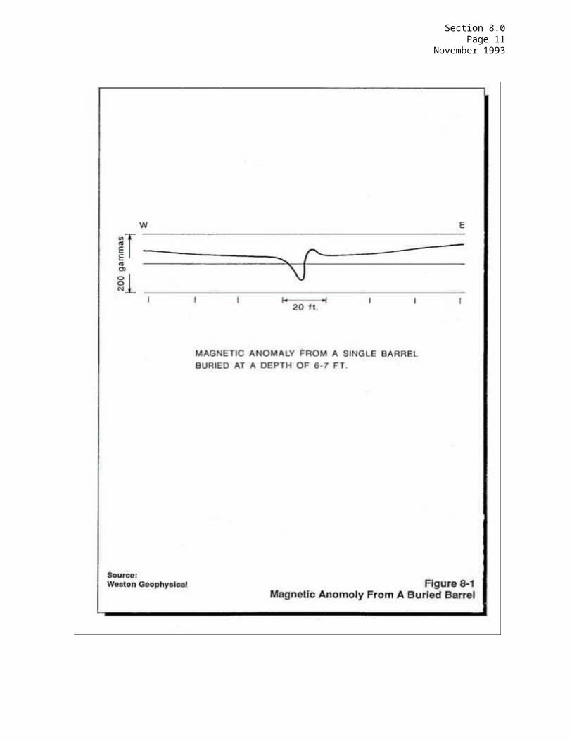
Section 8.0Page 12
November 1993
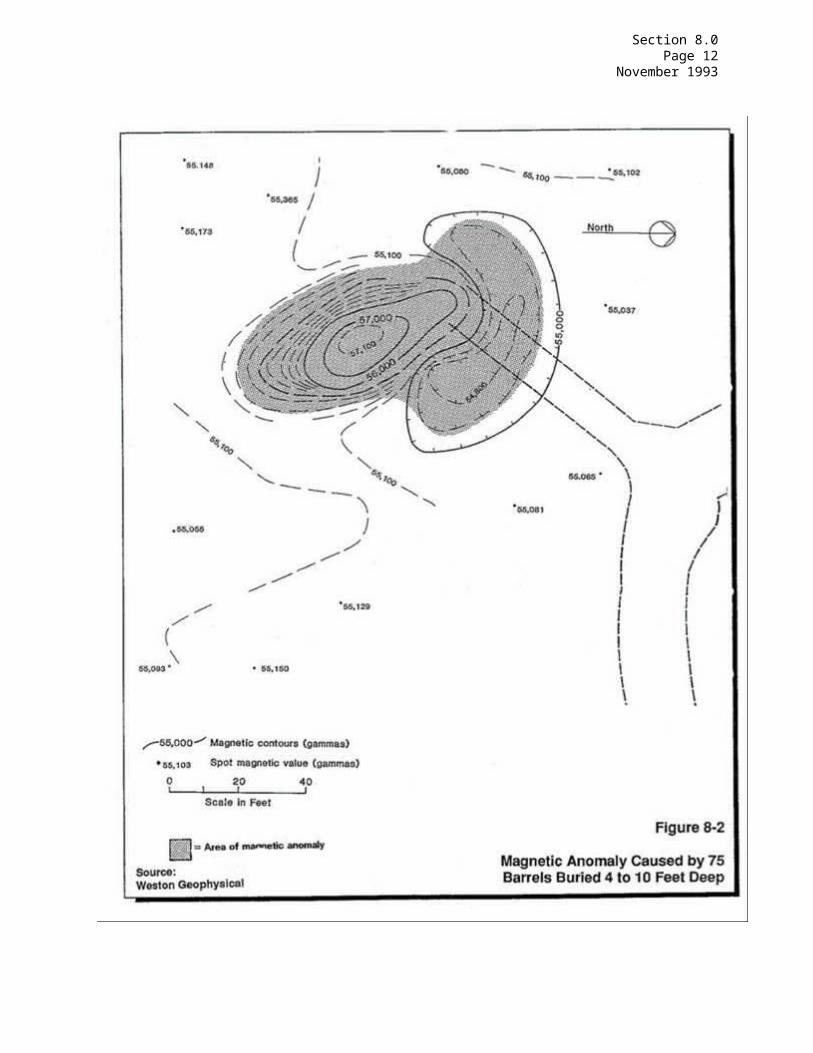
COMMONWEALTH OF MASSACHUSETTS
DEPARTMENT OF ENVIRONMENTAL PROTECTION
STANDARD REFERENCES FOR GEOPHYSICAL INVESTIGATIONS
SECTION 9.0 GRAVITY METHOD
Section 9.0Page i
November 1993
SECTION 9.0GRAVITY METHOD
TABLE OF CONTENTS
Section Title Page No.
9.1 OVERVIEW......................................... 1
9.2 INTRODUCTION..................................... 1
9.3 APPLICATIONS AND USES............................ 2
9.4 EQUIPMENT........................................ 2
9.5 FIELD PROCEDURES................................. 3
9.6 INTERPRETATION .................................. 4
9.6-1 Data Analysis.................................... 4
9.6-1.1 Instrument Drift and Earth-Tide Variations....................................... 5
9.6-1.2 Elevation Correction............................. 59.6-1.3 Bouguer Slab Correction.......................... 59.6-1.4 Latitude Correction.............................. 59.6-1.5 Terrain Correction............................... 69.6-1.6 Theoretical Gravity.............................. 6
9.6-2 Presentation of Results.......................... 69.6-3 Interpretation................................... 7
9.7 ADVANTAGES AND LIMITATIONS....................... 8
9.8 GLOSSARY......................................... 9
REFERENCES ................................................. 10
Section 9.0Page ii
November 1993
LIST OF FIGURES
Figure Title Page No.
9-1 Operation of LaCoste and Romberg Gravimeter (Schematic).....................................12
9-2 Contour Maps Illustrating Negative Gravity Anomalies.......................................13
9-3 Gravity Anomaly and Non-unique Solutions........14
Section 9.0Page 1
November 1993
9.0 GRAVITY METHOD
9.1 OVERVIEW
The gravity survey method is a passive geophysical technique which measures extremely small variations in the earth's gravitational field using a highly sensitive instrument. In gravity exploration the variation in density of the surveyed area is the only significant factor. Lateral variations in the distribution of mass in the earth's crust produce distortions or differences in the gravitational field. Tectonics, faulting, erosion, deposition, and other geologic movement involving rock often result in lateral density variations in the subsurface rocks. Measured gravitational differences are interpreted in terms of probable subsurface mass distributions, which are inferred from surface and near surface geologic conditions. Typical applications for this method may include locating variable fill conditions, bedrock knobs or depressions, and subsurface cavities or voids.
A gravity method which may be useful to characterize sites prior to drilling test wells is referred to as the "microgravity" method. This method produces data which allows more detailed or higher resolution interpretation than ordinary gravimetric measurements taken on a regional scale. The detailed resolution of the microgravity survey is more suited to the limited areal surveys associated with environmental investigations.
9.2 INTRODUCTION
The gravity method is one of the older geophysical methodologies that, as the name implies, measures changes in the gravitational field of the earth. This method is quite sensitive to a number of variables such as elevations of individual stations, elevations of surrounding topography, and local density variations that might be caused by excavation and backfilling.
Observed gravity measurements are variations in the earth's true gravitational attraction from one location on the earth's surface to another. Spatial variations in the value of observed gravity depend upon a number of factors including:
o Lateral density variations of earth materials in the vicinity of an observation point.
o Elevation
o Latitude
o Surrounding terrain variations (topography)
o Tidal fluctuations
The unit of gravitational measurement is a "gal" which is equal to the
Section 9.0Page 2
November 1993
force which will cause a mass to be accelerated one centimeter per second per second (cm sec-2). The acceleration of gravity at the earth's surface is approximately 980 gals. In gravity exploration work, variations as small as one ten-millionth of the earth's field can be detected with gravimeters. The measurement unit used in exploration gravity surveying is the milligal (10-3 gals). Microgravimeters are extremely sensitive instruments that can detect variations of exceptionally small magnitude; they are measured in units of microgals (10-6 gals).
The following sections cover various practical aspects of the gravity method and further explain some of the inherent difficulties with routine usage of this technique.
9.3 APPLICATIONS AND USES
Microgravity measurements can be used to detect the following conditions:
o Joint and fracture zones
o Dissolutions
o Collapses
o Cavities
o Buried river channels
o Fault scarps
9.4 EQUIPMENT
The LaCoste-Romberg and Worden gravimeters are available commercially.
The LaCoste-Romberg Model D is the only commercially available microgravimeter. These instruments measure the elongation of a spring which supports a weighted beam. An increment of elongation of the spring is proportional to an increment of gravity. The LaCoste-Romberg gravimeter is heated to maintain a constant instrument temperature and, consequently, a more sensitive and stable reading. The principle of operation of a LaCoste-Romberg microgravimeter is illustrated in Figure 9-1.
Some instruments are not temperature-controlled and instrument temperatures must be noted and a correction made for each reading. Gravimeters with heaters require a portable energy source (batteries) and must have an appropriate warm-up time (approximately one day) to acquire stable, accurate readings.
Section 9.0Page 3
November 1993
9.5 FIELD PROCEDURES
The operation of the instrument is rather straightforward, but acceptable levels of accuracy require meticulous attention to details, such as:
o Instrument leveling
o Surveyed location
o Surveyed elevation
o Instrument drift
o Time of measurement
Elevation and location survey accuracies of at least one-tenth of a foot of elevation, and approximately 2 feet horizontally are required for a microgravity survey. The topographic survey can be performed before, during, or after the gravity measurements.
The high level of accuracy required in gravity surveys dictates repeated readings at a base station (survey point) throughout the period of the survey to compensate for time variations (drift) inherent in all instruments. Typically, base station readings are taken at least three times a day and often are repeated in one-hour intervals. The practice of beginning and ending a series of location measurements at the same point (or base station) is referred to as "looping".
Initially, short loop times are necessary to minimize errors due to mechanical adjustments caused by the instruments internal thermal stress. Loop times for microgravity instruments that have been recently reheated to operating temperatures should be initially at about 30-minute intervals. Loop times can then get progressively longer up to a maximum of one hour.
At each station the gravimeter is set on a metal tripod which provides a stable base. The instrument is leveled by two horizontal and mutually-perpendicular levels in the instrument. Microgravity instruments which incorporate 30-second fluid levels should be employed rather than instruments which are equipped with 60-second levels. The 30-second levels provide a more precise leveling accuracy.
The gravimeter itself can be operated by a single operator. Three readings are commonly taken at each station, checking levels between readings to ensure data quality and minimize operator error.
Important information that should be recorded in field note books includes:
o Instrument number
o Date and time of reading
o Operator
Section 9.0Page 4
November 1993
o Station identification number
o Base station
o Instrument readings
To assure correlation between data sets, the relative gravity for each base station can be established by incorporating Absolute Base Stations, which are part of an international gravity network adjusted to the 1979 Potsdam value, in the survey loop. A listing of Absolute Base Station locations can be obtained from NOAA in Washington, D.C.
Gravity stations are arranged either in gridded survey patterns or in linear traverses. Gridded survey patterns provide more detailed information, but at a higher cost due to the higher number of stations. When considering the locations of gravity stations, precautions should be taken whenever possible to avoid areas with major topographic changes (i.e., greater than 50 feet). These topographic changes affect gravity measurements because of the upward attraction of hills or lack of downward attraction by a valley. Earthquakes and other vibratory phenomena can also adversely affect gravity readings. Generally, when an earthquake has occurred the instrument reading beam may drift and cannot be stabilized. Depending on the distance to and magnitude of the earthquake, gravity measurements should be suspended for a few hours or until the next day. Another potential problem in conducting a gravity investigation is unstable ground materials such as loose sand, nearby sources of vibration (e.g., heavy truck traffic and construction equipment) or stone ballast. Generally, these conditions can be overcome with patience, slight changes in station locations or altering the time of day that the investigation is conducted (i.e., taking measurements at the conclusion of heavy traffic). 9.6 INTERPRETATION
Although gravity data ("raw data") are readily acquired by a trained instrument operator, a number of processing/connection steps must occur before an interpretation can be performed. This aspect of gravity measurements is in marked contrast to magnetic measurements wherein the field recorded magnetic data are directly useful.
9.6-1 Data Analysis
Gravity data obtained in the field should be corrected for:
o Instrument drift
o Earth tide variations
o Elevation (Free-air)
o Bouguer slab
o Latitude
Section 9.0Page 5
November 1993
o Influence of surrounding topographic (terrain) variations
o Theoretical gravity
9.6-1.1 Instrument Drift and Earth Tide Variations
The observed gravity for each station is determined by looping a base station with a known gravity value and correcting readings for instrument drift and earth tide variations. Instrument drift and earth tide variations are calculated by dividing the difference in the base station readings (end of loop minus beginning of loop) by the time required to complete the loop. Each station reading is then corrected by adding the drift factor calculated for each station. Observed gravity values are then calculated by multiplying the corrected meter reading difference between the base and the gravity station by factors unique to the particular gravity meter.
9.6-1.2 Elevation (Free-air) Correction
To eliminate the effect of elevation differences on data collected during a gravimetric survey, all gravity stations within a common data set must be corrected to a common elevation datum plane. Sea level is the most commonly used datum plane. The normalization of survey points to sea level actually involves two corrections, the Elevation (free-air) correction and the Bouguer Slab (Section 9.6-1.3) correction.
The free-air correction compensates for the fact that the attraction of gravity above sea level decreases with increasing elevation. This inverse relationship is due to the fact that as elevation increases so does the distance from the earth's center. When the gravity stations are above the datum plane, the free-air corrections are added to the observed gravity values.
9.6-1.3 Bouguer Slab Correction
The Bouguer Slab correction is the second step in the normalization of gravimetric survey data to sea level. The Bouguer correction removes the gravimetric effect of the material present between the survey elevation and the sea level reference point. Bouguer corrections are made assuming a slab of infinite horizontal extent, constant density and constant thickness.
A commonly used slab density in New England is 2.67 g/cm3, which is the approximate density of the granitic crust. Bouguer corrections are applied in the opposite sense of the free-air corrections, that is, they are subtracted from the observed instrument response when the station is above the common datum plane.
9.6-1.4 Latitude Corrections
Latitude corrections compensate for the centrifugal acceleration due to the rotation of the earth and the variation of the earth's radius between
Section 9.0Page 6
November 1993
the poles and equator. Maximum latitude corrections occur at latitude 45 where the variation is approximately 0.01 milligals per 40 feet of north-south displacement.
The International Gravity Formula of 1967 incorporates the latitude correction in the calculation of theoretical gravity.
9.6-1.5 Terrain Correction
Terrain corrections are applied to the gravity data when the topography of the surveyed area is not relatively flat. The presence of nearby hills will result in an upward component of gravity that partially counteracts the downward pull exerted by the rest of the earth. Nearby valleys below the elevation station of the survey will cause an apparent loss of mass between the station and datum elevation to be observed. Both effects diminish the measured gravitational field; therefore, the terrain correction is always added to the data. Terrain corrections are calculated using the slab density used in the Bouguer slab correction. There are several graphical methods for calculating terrain corrections. All require a good topographic map of the area at a minimum of a 10-foot contour interval. The most commonly used graphical method uses templates that divide the area into zones for which the average elevation can be estimated and the terrain correction calculated. Tables of terrain corrections developed by Hammer (1939), facilitate this operation considerably (Telford 1976).
9.6-1.6 Theoretical Gravity
The difference between the corrected station gravity and the calculated theoretical gravity for each station is the Bouguer gravity. Theoretical gravity values are calculated using station latitudes and a relationship adopted by the International Association of Goedesy.
9.6-2 Presentation of Results
The results of a gravity survey can be presented either as contour maps or as profiles depending upon the data processing and/or interpretation techniques. Data presentation formats include: a raw-data map, which presents the gravity readings that have been corrected for instrument drift and earth-tide effects; a free-air gravity map, which presents the raw data corrected for station elevations (reduced to a common elevation datum); a simple Bouguer map, which presents the free-air gravity values corrected for the Bouguer slab; a complete Bouguer map, which presents simple Bouguer values corrected for terrain variations; and a residual anomaly map, which is a plot of the residual gravity values after regional gravity effects have been removed.
Data processing procedures to prepare each of the above-mentioned maps include assumptions that may or may not be true and may bias the interpretation of the gravity data. Therefore, the preparation and qualitative analysis of each map may be necessary to identify any bias or anomalies that have been created due to the data processing.
Section 9.0Page 7
November 1993
Interpreted gravity results are presented as 2-D, 2-1/2-D or 3-D profiles or maps. The 2-D results assume infinite lengths in the 3rd dimension, 2-1/2-D results have a finite length in the 3rd dimension and 3-D modeling results have 3-dimensional geometric shapes.
9.6-3 Interpretation
The complete Bouguer anomaly map represents the contribution to the resultant gravity value of all earth materials that exist beneath the ground surface after all corrections have been made. A Bouguer anomaly map (Figure 9-2), looks very much like a topographic contour map. Bouguer anomalies are interpreted in terms of the size, shape, and position of the subsurface structures. The first step in the interpretation of the complete Bouguer gravity data is known as regional residual separation. Regional residual separation is performed to identify the anomaly components arising from sources of small lateral extent (which are usually the anomalies of interest) from the sources of great lateral extent (i.e., regional geologic features). In such a situation, the large anomaly can be considered to have a low spatial frequency (equivalent to a large lateral extent or a long wavelength) and the small anomaly a high spatial frequency (corresponding to a short lateral distance or wavelength). The most common objective in such cases is to isolate the anomaly associated with the smaller source. The residual data can be separated from the regional data in a number of ways. The averaging method, polynomial fitting, and upward continuation and wavelength filtering regional residual separation methods are a few. Textbooks, such as Telford (1976) and Nettleton (1976) explain in detail regional residual separation methods.
There is extensive literature on the subject of and significant problems involved in regional residual separation. The techniques listed above are some of the more common techniques used. The choice of the method used for removing the regional residual depends upon many factors, the most important being the total labor involved, the complexity of the gravity map, the density and distribution of the stations and quality of the data. The residual gravity maps are a by-product of the regional residual separation. These maps are used to predict the physical characteristics and proximity of near-surface anomalous bodies.
Before a quantitative interpretation is attempted, a qualitative analysis of the data should be made to determine the presence of anomalous sources and to get a general idea of the depth, strike, and density of sources. Qualitative analysis includes an evaluation of the polarity, magnitude, gradient, and trends of residual anomalies as well as a comparison with other available geophysical (e.g., magnetic, seismic, and electrical) and geological data.
Based on the qualitative analysis of the regional map, a quantitative interpretation to determine possible individual sources of the anomalies can be undertaken. The quantitative interpretations are accomplished using 2- and 3-dimensional computer modeling techniques. Each anomaly is assigned a geometric shape and density value. All gravity
Section 9.0Page 8
November 1993
interpretations benefit from incorporation of geologic constraints. Such constraints can come from surface geology, geomorphology, subsurface geology, boring logs, seismic reflection and refraction data, magnetic surveys, and geochemical data.
For a given distribution of gravity there is not a unique solution that corresponds to the observed gravity. That is, for a given width of anomaly there is a corresponding maximum depth and a cone of possible sources, as illustrated in Figure 9-3.
9.7 ADVANTAGES AND LIMITATIONS
Advantages
The advantages of a gravity survey are:
o Field work can be carried out by one to three persons in any accessible area, including highly developed urban and industrialized sites, over pavements, fills, landfills, on lake ice, and inside buildings.
o Instrumentation is portable; the work can be silent and produce no visible disturbance to an environment other than stakes or other station markings.
o The method lends itself well to areal coverage; contour maps of bedrock or other features have obvious advantages over information at points or along profiles.
Limitations
The instruments used to measure the gravitational field are expensive, complex, and sensitive to use.
The increase in sensitivity of the "Microgravity" method creates logistical problems including: a greater need for more detailed elevation data; a "quiet" site with regard to background vibrations that might affect the microgravimeter; as well as some inherent stability problems for the instrument itself.
The other limitations of a gravity survey are:
o Applications are limited to mapping of density-dependent interfaces.
o Accurate station locations and elevations are necessary.
o Calibration with geological "knowns" such as outcrops, borings, or seismic profiles is necessary for quantitative work.
o Excessive topography, access problems, and certain bedrock complexities may seriously limit the accuracy of data interpretation.
Section 9.0Page 9
November 1993
9.8 GLOSSARY
Anomaly - A deviation from an expected condition or response.
Bouguer anomaly or complete Bouguer anomaly - Gravity value after the observed (measured) gravity has been corrected for latitude, free-air, Bouguer slab, and terrain.
Bouguer slab - An imaginary slab of infinite horizontal extent, constant density and thickness
Earth tides - Variations in the gravitational attraction of the sun and the moon as their positions change with respect to the earth, (maximum amplitude of 0.3 gal occurring in a period as short as an hour).
Gal - The unit of gravitation measurement. A force which will cause a mass to be accelerated one centimeter per second per second.
International gravity value - An equation that accounts for the fact that the earth is not a perfect sphere, but is more like a perfect fluid for which balance is maintained between the gravitational forces tending to make it spherical and the centrifugal forces of rotation tending to flatten it. As a result the equatorial radius is approximately 21 km greater than the polar radius.
Mass - The volume of an object times the density of the object.
Raw data - The observed values noted during data acquisition, but requiring several "connections" before a meaningful profile or contour map can be prepared.
Residual gravity map - Resulting gravity map after regional gravity effects are removed from Bouguer anomaly values.
Simple Bouguer anomaly - Gravity value after the observed (measured) gravity has been corrected for latitude, free-air, and Bouguer slab.
Section 9.0Page 10
November 1993
REFERENCES
Beck, A.E., 1981, Physical principles of exploration methods: London, England, MacMillan Press, Ltd., 234 p.
Dobrin, M.B., 1976, Introduction to Geophysical Prospecting: New York, NY, McGraw-Hill, 630 p.
Grant, F.S., and West, G.F., 1965, Interpretation theory in applied geophysics: New York, NY, McGraw-Hill, 583 p.
Hammer, S., 1939, Terrain corrections for gravimeter stations: Geophysics, v. 4, p. 184-94.
LaCoste and Romberg, Inc., Instruction manual for LaCoste and Romberg, Inc., Model G Geodetic Gravity Meter: Austin, TX, 14 p.
Nettleton, L.L., 1973, Elementary gravity and magnetics for geologists and seismologists: Tulsa, OK, Society of Exploration Geophysicists, Monograph no. 1, 121 p.
____, 1976, Gravity and magnetics in oil prospecting: New York, NY, McGraw-Hill, 453 p.
Talwani, M., Worzel, J.L., and Landisman, M., 1959, Rapid gravity computations for two-dimensional bodies with application to the Mendocino submarine fracture zone: Journal of Geophysical Research, v. 64, no. 1, p. 49-57.
Telford, W.M., Geldart, L.P., Sheriff, R.E., and Keys, D.A., 1976, Applied geophysics: New York, NY, Cambridge University Press, 860 p.
Texas Instruments, 1982, Worden gravity meter operating instructions: Houston, TX, 40 p.
Van Blaricom, Richard, 1980, Practical geophysics: Spokane, WA, Northwest Mining Association, 236 p.
Section 9.0Page 11
November 1993
SECTION 9GRAVITY METHOD
LIST OF FIGURES
Figure Title Page No.
9-1 Operation of LaCoste and Romberg Gravimeter (Schematic).....................................12
9-2 Contour Maps Illustrating Negative Gravity Anomalies.......................................13
9-3 Gravity Anomaly and Non-unique Solutions........14
Section 9.0Page 12
November 1993
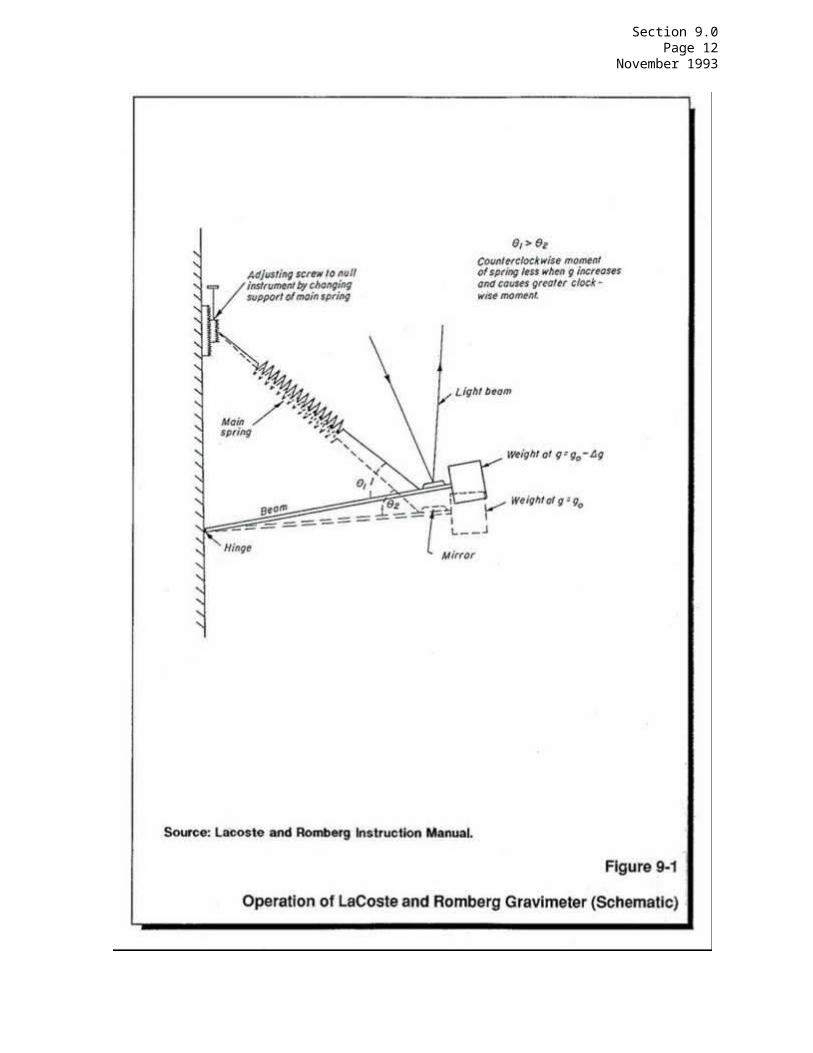
Section 9.0Page 13
November 1993
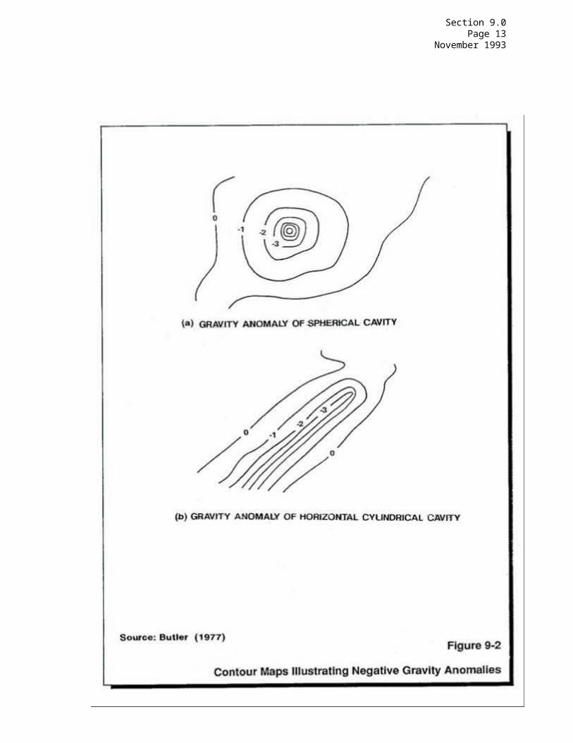
Section 9.0Page 14
November 1993
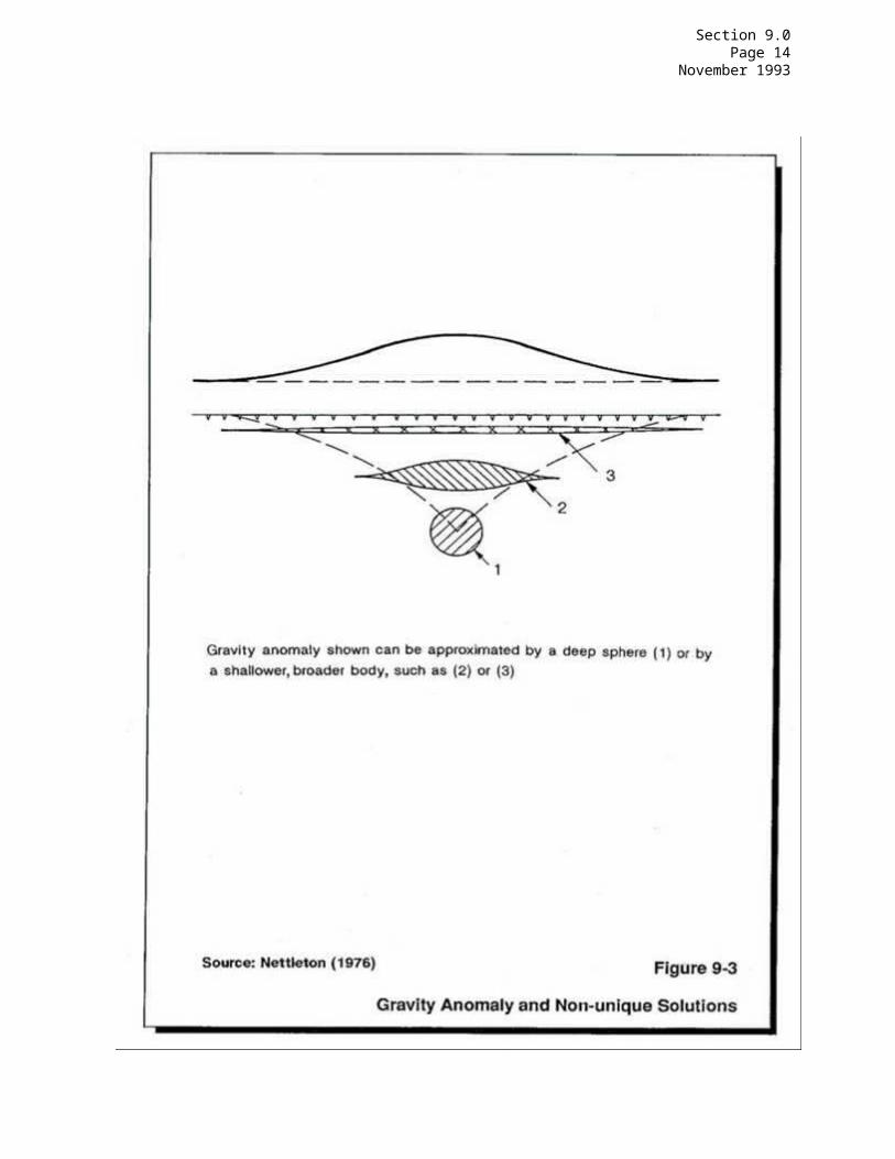
COMMONWEALTH OF MASSACHUSETTS
DEPARTMENT OF ENVIRONMENTAL PROTECTION
STANDARD REFERENCES FOR GEOPHYSICAL INVESTIGATIONS
SECTION 10.0 BOREHOLE GEOPHYSICAL METHODS
Section 10.0Page i
November 1993
SECTION 10.0BOREHOLE GEOPHYSICAL METHODS
TABLE OF CONTENTS
Section Title Page No.
10.1 OVERVIEW......................................... 1
10.2 INTRODUCTION..................................... 2
10.2-1 Equipment ....................................... 310.2-2 Field Procedures................................. 4
10.3 PASSIVE BOREHOLE METHODS (NON-PENETRATING)....... 5
10.3-1 Borehole Television Camera Surveys............... 5
10.3-1.1 Principles of Operation.......................... 610.3-1.2 Applications..................................... 610.3-1.3 Equipment........................................ 610.3-1.4 Field Procedures................................. 710.3-1.5 Interpretation................................... 710.3-1.6 Advantages and Disadvantages..................... 7
10.3-2 Caliper Logging.................................. 7
10.3-2.1 Principles of Operation.......................... 710.3-2.2 Applications..................................... 810.3-2.3 Equipment........................................ 810.3-2.4 Field Procedures................................. 810.3-2.5 Interpretation................................... 810.3-2.6 Advantages and Disadvantages..................... 8
10.3-3 Temperature Logging.............................. 9
10.3-3.1 Principles of Operation.......................... 910.3-3.2 Applications..................................... 910.3-3.3 Equipment........................................ 910.3-3.4 Field Procedures................................. 1010.3-3.5 Interpretation................................... 1010.3-3.6 Advantages and Limitations....................... 10
Section 10.0Page ii
November 1993
SECTION 10.0BOREHOLE GEOPHYSICAL METHODS
TABLE OF CONTENTS (continued)
Section Title Page No.
10.3-4 Self Potential (SP)............................11
10.3-4.1 Principles of Operation........................1110.3-4.2 Applications...................................1110.3-4.3 Equipment......................................1110.3-4.4 Field Procedures...............................1210.3-4.5 Interpretation.................................1210.3-4.6 Advantages and Disadvantages...................12
10.3-5 Fluid Resistivity..............................12
10.3-5.1 Principles of Operation........................1210.3-5.2 Applications...................................1310.3-5.3 Equipment......................................1310.3-5.4 Field Procedures...............................1310.3-5.5 Interpretation.................................1310.3-5.6 Advantages and Limitations.....................14
10.3-6 Inhole Flow Measurement (Flowmeters)............15
10.3-6.1 Principles of Operation........................1510.3-6.2 Applications...................................1510.3-6.3 Equipment......................................1610.3-6.4 Field Procedures...............................1610.3-6.5 Interpretation.................................1710.3-6.6 Advantages and Limitations.....................17
10.4 FORMATION PENETRATING METHODS..................18
10.4-1 Resistivity Techniques.........................18
10.4-1.1 Principles of Operation........................1810.4-1.2 Applications...................................1910.4-1.3 Equipment......................................1910.4-1.4 Field Procedures...............................2010.4-1.5 Interpretation.................................2010.4-1.6 Advantages and Disadvantages...................21
Section 10.0Page iii
November 1993
SECTION 10.0BOREHOLE GEOPHYSICAL METHODS
TABLE OF CONTENTS (continued)
Section Title Page No.
10.4-2 Acoustic (Sonic) Methods........................22
10.4-2.1 Principles of Operation.........................2210.4-2.2 Applications....................................2310.4-2.3 Equipment.......................................2510.4-2.4 Field Procedures................................2510.4-2.5 Interpretation..................................2510.4-2.6 Advantages and Disadvantages....................26
10.4-3 Nuclear (Radiation) Methods....................27
10.4-3.1 Principles of Operation........................27
10.4-3.1.1 Natural Gamma-ray Log..........................2710.4-3.1.2 Gamma-gamma Log................................2710.4-3.1.3 Neutron-epithermal-neutron Log 27
10.4-3.2 Applications....................................2810.4-3.3 Equipment.......................................2810.4-3.4 Field Procedures.................................2910.4-3.5 Interpretation..................................2910.4-3.6 Advantages and Disadvantages.....................30
10.4-4 Vertical Seismic Profiling (VSP).................31
10.4-4.1 Principles of Operation..........................3110.4-4.2 Applications....................................3210.4-4.3 Equipment.......................................3210.4-4.4 Field Procedures.................................3310.4-4.5 Interpretation..................................3310.4-4.6 Advantages and Disadvantages.....................34
10.5 GLOSSARY........................................34
REFERENCES ...............................................36
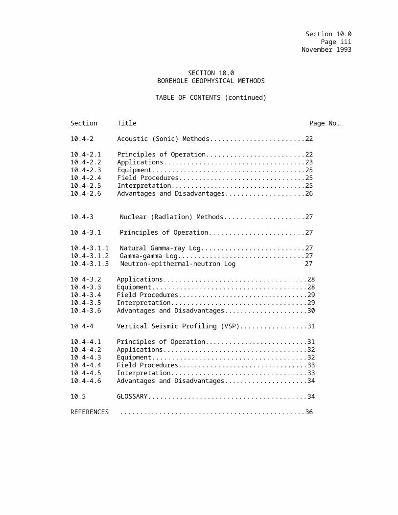
Section 10.0Page iv
November 1993
SECTION 10.0BOREHOLE GEOPHYSICAL METHODS
LIST OF FIGURES
Figure Title Page No.
10-1 Typical Geophysical Logging Setup...............41
10-2 Caliper Probes ................................42
10-3 Interpretation of Borehole Temperature Profiles.......................................43
10-4 SP Log Example.................................44
10-5 Example of Flowmeter Log.......................45
10-6 Resistivity Probes.............................46
10-7 F versus φ Plot for Sandstones.................47
10-8 Acoustic Velocity Logging......................48
10-9 Acoustic Televiewer Diagram....................49
10-10 Example of Acoustic Televiewer Image............50
10-11 Example of Cross-plot of Acoustic Velocity and Neutron Logs with Geologic Interpretation.................................51
10-12 API Gamma Ray Units for Various Tertiary Sediments......................................52
10-13 Tube Waves Generated by Seismic Energy Incident on Permeable Fracture Zones............53
10-14 VSP to Determine 3D Geometry of Strata, Moduli Values and Permeability.................54
10-15 Relationship Between Hydraulic Conductivity and Ratios of Tube Wave to P Wave Amplitudes as a Function of Frequency.....................55
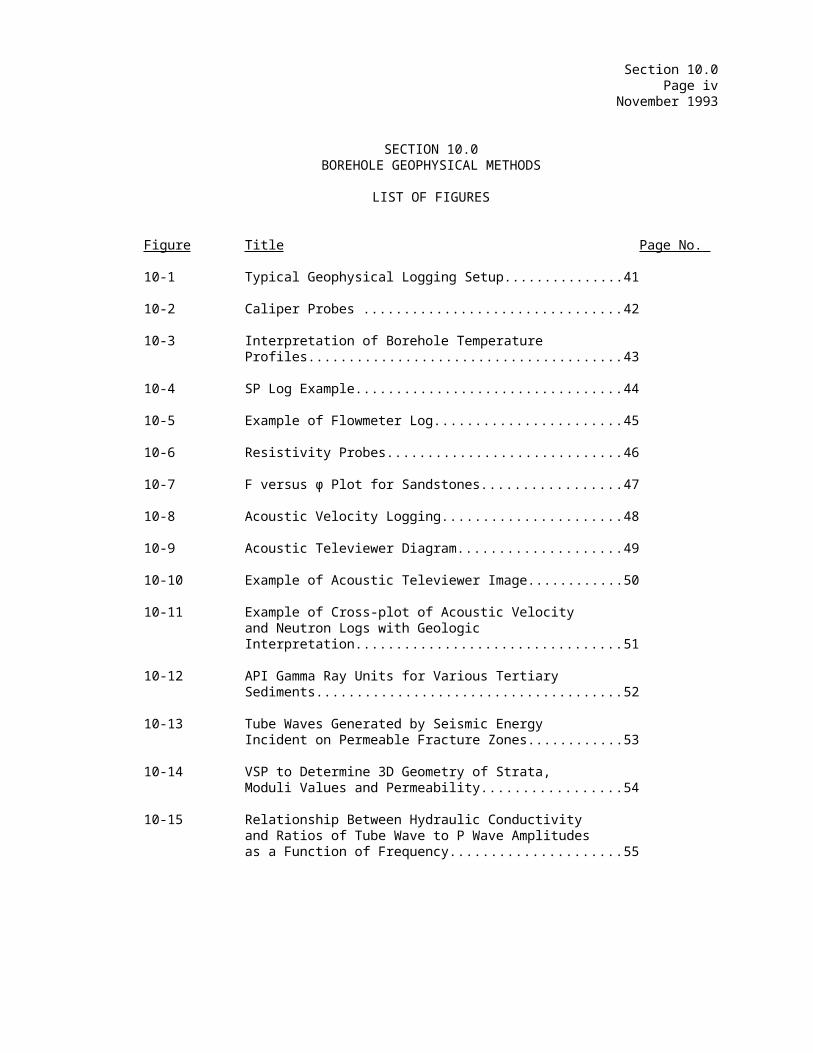
Section 10.0Page v
November 1993
SECTION 10.0BOREHOLE GEOPHYSICAL METHODS
LIST OF TABLES
Table Title Page No.
10-1 Common Borehole Logging Techniques..............57
10-2 Compressional and Shear Velocities in Rocks.....58
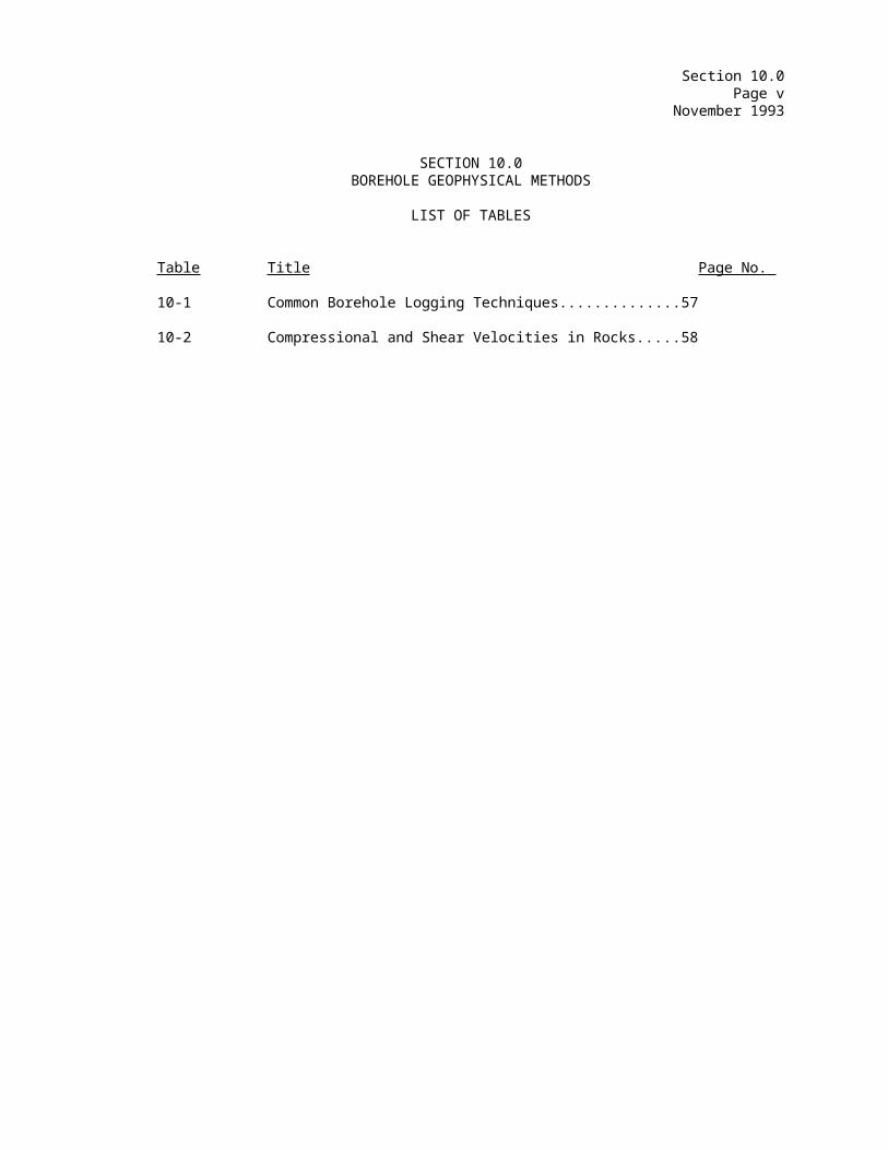
Section 10.0Page 1
November 1993
10.0 BOREHOLE GEOPHYSICAL METHODS
10.1 OVERVIEW
Borehole surveys are designed to provide a continuous vertical profile of the soil, rock and water conditions immediately adjacent to the borehole. Logging is accomplished by lowering probes into the borehole to measure the electrical, acoustical, or radioactive properties of the materials surrounding a borehole. The surveys are non-destructive and can often be run in existing boreholes, monitoring wells, and water wells with no modifications.
Borehole geophysical methods are used primarily to characterize rocks, correlate overburden or rock units, and determine physical and hydrologic properties. Table 10-1 provides a listing of the applications for the methods described in this section. Specific applications include determining porosity, locating clay layers, determining water quality, estimating permeability, and finding fracture zones and zones of water loss or gain. More detailed discussion of the theory and interpretation of the use of borehole geophysical methods in groundwater investigations is presented by Keys and MacCary (1971), Kwader (1982), and Collier and Alger (1988).
The primary advantage of borehole methods is that they provide an unbiased, high density of measurements of soil, rock and water properties at precise depths. Borehole methods are fast and generally unaffected by surface features such as power lines, buildings and railroad tracks. Little data reduction is necessary before most logs can be interpreted; often preliminary interpretations can be made as they are being run. Borehole logging is non-destructive and can often be run with no modifications in existing cased or uncased boreholes and in the screened and unscreened intervals of monitoring wells.
Some borehole methods, such as the temperature log (a log is the printed display of the parameter being measured vs. the depth where the measurement is taken), the caliper log, and the flowmeter log are relatively simple to operate and the data recordings are easy to interpret.
Other methods, such as logging with an active nuclear source and resistivity logging are much more complex for operation and/or for data interpretation. Borehole geophysical logging of such methods is a technical speciality that requires complex electronic equipment to be operated according to exact design specifications. Since no two boreholes exhibit the same geophysical response, and as responses can not be quantitatively validated during logging, the quality of a log depends strongly on the operator's experience and judgment.
The radius of investigation for most probes is commonly less than one foot. Depending on the permeability of the formation and the drilling techniques applied, the condition of materials investigated may be altered by the drilling method. The borehole surveys may therefore
Section 10.0Page 2
November 1993
provide only limited representation of true formation properties.
Borehole geophsyical methods may not be cost-effective for typical environmental investigations in Massachusetts, where shallow overburden wells dominate. Borehole geophsyical methods are bested suited for deep bedrock wells, where the information gathered will be the most useful. When natural in-situ conditions are present, and several deep boreholes are logged and correlated, often very large areas can be geologically characterized with a minimum of time and cost.
10.2 INTRODUCTION
Borehole geophysical techniques (also called logging) are a group of active and passive geophysical methods used to provide detailed physical properties of soil, rock, and water. The term "active" implies subjecting the area around and in the borehole to a stress (either electric, thermal, acoustic, etc.) in which a response can be measured (formation-penetrating methods), while "passive" involves measuring only naturally-occurring conditions (non-penetrating methods).
Table 10-1 shows the array of available borehole techniques keyed to types of subsurface information desired and limitations posed by borehole conditions. Many of the techniques are based on counterpart surface geophysical methods, adapted to the borehole environment. Typically, these adaptations include the reduction of equipment size (the probes for most techniques will fit inside a 2-inch diameter hole), reduction and standardization of the fixed source to receiver spacing (and sometimes a corresponding reduction in the depth of investigation), protection of probes from pressure and temperature effects, and interpretation of data with respect to vertical rather than horizontal changes.
Borehole geophysical logging methods to be discussed are:
o Downhole television camera
o Caliper
o Temperature
o Electrical methods (Single-point-resistance, Normal resistivity, SP, Fluid resistivity, Electromagnetic/Induction)
o Flowmeter
o Acoustic methods (Velocity, Waveform, Acoustic televiewer)
o Nuclear methods (Natural gamma, Neutron, Gamma-gamma)
o Vertical seismic profiling
Use of more than one logging technique is generally necessary to determine soil and water properties adjacent to the borehole. Because
Section 10.0Page 3
November 1993
each probe has a different response, these logs are interpreted by cross-comparisons to determine specific characteristics of interest. For example, caliper, single-point resistance, acoustic and thermal logs may be run as a suite to identify fracture zones in rock.
10.2-1 Equipment
Figure 10-1 shows a typical geophysical logging set up. The surface and downhole equipment used in borehole geophysical surveys is connected by the logging cable. The cable provides transmission of electrical power to the downhole probe and a return path for signals generated in the probe. Cables are usually one- or four-conductor, insulated, wire-wrapped (shielded), and chemically stable.
Equipment on the ground surface at the hole includes:
o Power supply (AC or DC)
o Instrument and probe controls (on/off, open/close caliper, scale setting)
o Winch and depth counter
o Signal receiving and conditioning circuits
o Recorder and/or portable computer
o Well head cable tripod or sheave
Downhole equipment includes the measuring probe which is connected to the cable by a threaded water-tight coupling. Two or more logging methods can occasionally be performed with the same probe (e.g., SP and normal resistivity). Probes can be changed quickly so that a number of logs can be performed at one borehole with minimal down-time.
Some logging systems are equipped with digital data acquisition systems connected to portable personal computers. Data are sampled at regular intervals (usually six inches or one foot) and stored on magnetic tape or disk. This setup is highly desirable because digital data can be manipulated easily for calculations or presentation. Although tedious, analog data can be digitized at the office using available digitizing hardware and software.
Section 10.0Page 4
November 1993
10.2-2 Field Procedures
Field procedures for logging generally consist of six steps, as outlined below:
o Equipment setup and assembly
o Verification (or calibration) of probe functions at surface
o Downhole run and total depth determination
o Main run (uphole as appropriate)
o Repeat run (if verification of anomalies warrants)
o After-run calibration
Calibration measures the probe's response to a known standard. Checking the probe response against a known standard before and after a borehole survey ensures that the probe is operating and measuring correctly. After the probe response is calibrated, it is placed at the top of the borehole and the reference point of the probe is positioned at a reference elevation (usually ground surface or top of casing). The depth counter is then set to either zero or ground zero and the probe is lowered to the bottom of the hole. This process is known as depth calibration.
It is customary practice to make a record of log response when lowering most probes to the bottom, although a formal depth-registered log is normally not necessary or practical. However, it is important that the downhole run document the extremes in order to choose the optimal instrument settings for the uphole run, during which a formal depth-registered log is made. (Uphole and downhole recorded logs will not be identical for most geophysical probes because of probe design and delayed response in the direction of probe movement.)
The temperature and fluid resistivity probes are run from top to bottom so that the water in the borehole is not mixed or displaced appreciably by moving the probe. All other geophysical surveys are recorded during probe ascent in the borehole so that constant logging speed and cable tension can be maintained.
Once the probe reaches the bottom of the hole, the optimal instrument settings are activated, and the uphole log is made. The footage dial reading on the winch is recorded on the field chart (analog recorder paper) at the exact point of pen stoppage at the top of the hole to verify depth calibration. Agreement between pen and dial should be within 0.5 foot.
Analog recordings are usually made at a vertical (depth) scale of one inch equals 10 feet; however, a different scale may be used to show more detail, or less detail, if a digital recording is made simultaneously. If the data are not digitally recorded, it is very important to select
Section 10.0Page 5
November 1993
instrument settings that will result in nearly full chart-width pen fluctuation without reaching the margins of the chart paper. Generally, one set of instrument settings can be selected to achieve this result for the entire depth logged. All setting changes must be accurately documented on the chart (beside the change or in the header). If the log appears uncharacteristic or suspect, the probe calibration is checked. A second complete or partial log should be made if any doubts persist concerning instrument/probe response.
When contaminants are (or may be) present, the cable must be decontaminated as it is removed from the well. When multiple logs are to be run in shallow wells, it is desirable and usually possible to set up the logger at a distance adequate to prevent the wet cable from wrapping on the spool between runs. In this case, cable decontamination is needed only after the last probe is extracted. A preliminary rinse should be performed while the cable is over the borehole. One method for decontamination is to set up stations along the cable for washing and rinsing (for a more thorough discussion of decontamination procedures, see Sections 3.3 and 6.5 of Standard References for Monitoring Wells, MA DEP, WSC #310-91) as shown in Figure 10-1. Another method is to construct a jig to hold sponges and fluids for washing, or properly-attired field personnel can perform decontamination using spray bottles and sponges.
Downhole probes that will be in direct contact with potentially contaminated soil and water must be decontaminated between logging runs. Probes should also be thoroughly decontaminated, taking care to remove all contaminants from moving parts (e.g., hinges on caliper arms). Without decontamination, contaminants can be transferred onto the spool, contaminating the remainder of the cable or other boreholes.
Borehole methods that employ the use of radioactive sources should only be used in boreholes that are either cased or completed in competent bedrock. Operators of probes with radioactive sources must be certified and licensed by the United States Nuclear Regulatory Commission.
10.3 PASSIVE BOREHOLE METHODS (NON-PENETRATING)
10.3-1 Borehole Television Camera Surveys
Although the borehole television camera is not technically a geophysical logging method, it is discussed in this section because of its usefulness in the investigation of open hole bedrock wells and the evaluation of casing integrity.
10.3-1.1 Principles of Operation
A borehole television camera survey can be made of any well or boring of appropriate diameter that is filled with clear water or air. The camera, similar to a home video camera, is enclosed in a watertight, pressure-safe housing that contains a light source. A coaxial cable is attached
Section 10.0Page 6
November 1993
to the camera and the light source. The cable allows the transmission of power to the downhole instruments and the transmission of video signal from the camera. Video signals sent up the coaxial cable are viewed on a television monitor at the surface. The survey is also recorded on videotape to permit future analysis.
10.3-1.2 Applications
Borehole camera surveys are generally used for inspection of cased borehole sections. Camera surveys can reveal mechanical defects in casing such as:
o Cracks, holes and splits
o Oxidation (rust) of steel casing
o Scaling by contaminants
o Plugging of slots or screen
In an open hole, the borehole camera can assist in determining rock type, layering, the presence of fracturing, and hole integrity.
10.3-1.3 Equipment
A number of borehole camera systems are commercially available. These systems are generally composed of a downhole camera with light source, hand or light duty electric winch with coaxial cable, television monitor, camera control panel, and video tape recorder. Manufacturers' specifications and options, which may vary considerably among systems include:
o Probe size (1½-inch to 6-inch diameters are available)
o Black-and-white or color recording capabilities
o Size and quality of television monitor
o Camera lens quality (amount of distortion)
o Uphole remote controls (amount of light, focus, and aperture setting)
o Text and depth printed on log (recording)
Borehole cameras need a special coaxial cable for transmission of video data.
10.3-1.4 Field Procedures
Camera systems that do not have remote controls for adjustment of focus, amount of light or aperture must be lowered into the hole, checked for picture quality then removed and adjusted if necessary. The camera
Section 10.0Page 7
November 1993
system should be raised and lowered slowly in the borehole to avoid stirring up sediment that may have settled in slots, the screen, or on the bottom.
10.3-1.5 Interpretation
The visual inspection of a borehole or casing requires no special interpretation techniques.
10.3-1.6 Advantages and Disadvantages
The borehole camera can provide a very accurate picture of the mechanical condition of the boring and casing. Small features such as open fractures and clogged slots and screens can be observed with this technique.
Resolution of the camera varies considerably between manufacturers. The camera's resolution may not be high enough to show hairline fracturing.
Water clarity is usually a limiting factor in the use of borehole camera surveys. The possible effect of contaminants on the optical lens of the waterproof case should be considered before running a survey. Also, the borehole camera cannot be attached to a standard one- or four-conductor logging cable like those used for electrical, nuclear or caliper logging. 10.3-2 Caliper Logging
10.3-2.1 Principles of Operation
The caliper tool measures the diameter of the borehole. Spring-loaded arms, hinged to the probe body at their upper end, press against the borehole wall. The hinged end of the arm is connected to a variable resistor. As the arm moves out (in an enlarged section of the borehole), the resistance is lowered and a larger voltage is sent to the recorder and displayed is a change in borehole diameter. Figure 10-2 illustrates a three-arm and a four-arm caliper.
Section 10.0Page 8
November 1993
10.3-2.2 Applications
The caliper log is generally used to assess the variation in hole diameter for use in conjunction with other geophysical logging techniques that are sensitive to borehole size and smoothness (e.g., gamma-gamma, neutron, acoustic velocity). When appropriate, caliper log data may be used to determine corrections to other logs. Caliper logs can also be used to find fractures, solution channels, and vugs in hard rock, or to identify depths at which soft formations may be squeezing into the hole and substantially restricting other downhole testing.
10.3-2.3 Equipment
The most common and accurate of the caliper probes has three or four arms. Probes with four arms provide two diameters (maximum and minimum). The surface electronics contain opening and closing controls for the probe arms, as well as controls for calibration setting. Both the three and four arm models are calibrated using two different size rings of known diameter.
10.3-2.4 Field Procedures
No information can be obtained on the downhole run because the arms will not function properly in this direction. The caliper arms are opened at the bottom and a log is made pulling the probe uphole at a relatively slow rate of 8 to 15 feet per minute. In partially cased holes, the probe should be run in the casing to verify diameter calibration and check for major casing breaks, if this information is desired.
10.3-2.5 Interpretation
The interpretation of the caliper log is straightforward because the hole diameter is recorded directly in inches. Three-arm calipers tend to show the maximum hole size, while four-arm calipers will also show minimum hole size. Fractures, if they are non-vertical, show as sudden increases in borehole size. Fractures less than about 1/4 inch in aperture or those that intersect the borehole at a steep angle may not affect the position of the probe's arms, and go unrecognized.
10.3-2.6 Advantages and Disadvantages
The caliper tool gives a good indication of the rugosity (degree of roughness) of the borehole. Data are relatively simple to interpret and should always be run if logging an uncased borehole. The probe requires inspection and possibly cleaning of arm hinges before using to prevent a loss of sensitivity to diameter changes.
10.3-3 Temperature Logging
10.3-3.1 Principles of Operation
Section 10.0Page 9
November 1993
Temperature logging provides a vertical profile of temperature (or differential temperature) in a water-filled borehole. The probe is quite simple and features a thermistor (temperature-dependent resistor) mounted at its bottom end. The voltage across the thermistor is sent to the uphole circuits, voltage readings are converted to counts per second (cps) and cps fluctuation versus depth are recorded directly on the log. Each probe and surface electronics system has a laboratory-derived relationship between cps and temperature in degrees Celsius.
A more sensitive version of the temperature log, called the differential temperature log, is a calculation of the change in temperature between two points in the borehole. Differential temperature probes may contain two thermistors a fixed distance apart, or may contain one thermistor and calculate temperature changes electronically by comparing the present reading to stored data from previous readings.
10.3-3.2 Applications
The temperature log is used to help identify the source and movement of water in the borehole. The specific applications include:
o Location of zones of water flow
o Location of leaks in casing
o Identification of discrete aquifers
o Indication of permeability
Temperature logging can also be used to identify the location of cement outside the casing in a grouted hole if the probe is run within 24 hours of cementing.
10.3-3.3 Equipment
The equipment needed to run a temperature log includes a thermistor mounted on the end of the probe and protected by a thin metal cage, and a voltage-controlled recorder. The equipment is relatively simple to operate. The typical temperature probe can resolve differences in temperature of 0.02C, and high-resolution equipment can attain a precision of about 0.001C.
10.3-3.4 Field Procedures
The temperature probe should be the first log run in a borehole if it is to be included in the investigative suite. It should be run from top to bottom to avoid mixing of the water. It is especially important to run the differential temperature probe at a very slow and consistent speed (6
Section 10.0Page 10
November 1993
to 8 ft/minute is recommended) so that physical mixing of thermally stratified water will not occur.
Generally, the temperature probe is not field-calibrated. However, its calibration can be crudely checked in air or water if another temperature measuring device is available. The responsiveness of the probe and recorder electronics can be verified by breathing on the thermistor.
10.3-3.5 Interpretation
Normally, interpretation of the temperature log is based on the assumption that water in the well is at thermal equilibrium with the surrounding material. Water entering a well bore from different aquifers penetrated by the hole usually will have a different temperature and will cause a flattening or steepening of the log profile. Figure 10-3 demonstrates the standard interpretation of various configurations of temperature profiles. An abrupt anomaly on the log is caused by either warmer or cooler water entering or leaving the borehole at the depth of the anomaly. Permeable zones, especially major fractures and casing leaks, can thus be detected as anomalous points on the temperature logs if any groundwater movement is occurring.
10.3-3.6 Advantages and Limitations
A temperature log must be made in a fluid-filled hole. The preferred situation for most investigations requires that a borehole has reached thermal equilibrium with the surrounding material and that this equilibrium has not been disturbed by sampling or other downhole activities. Depending on subsurface permeabilities and the degree of thermal disturbance, the equilibration time can vary from a day to perhaps several weeks. In order for this log to reflect natural subsurface conditions, it is also necessary that surficial water does not enter the hole, and that the well construction grout (which gives off heat) has cured for at least three days.
A temperature log is often very informative for holes several hundred or more feet deep, especially where deeper aquifers or fractures exist that are hydraulically not directly connected to a shallow aquifer. The equipment is easy to operate and is relatively inexpensive.
The thermistors may be quite fragile, and downhole breakage can occur if the borehole has edges that may catch the probe.
10.3-4 Self Potential (SP)
10.3-4.1 Principles of Operation
Electrochemical potentials are generated by interactions between ions in the borehole water and pore water in the borehole wall. The Self Potential (SP) method is a passive technique which measures these naturally-occurring voltage potentials in the borehole.
Section 10.0Page 11
November 1993
More importantly, in geologic environments in which groundwater enters the borehole through thin permeable zones, voltage potentials can also be generated electrokinetically (creating streaming potentials) when an electrolyte (groundwater) flows through a porous medium (rock or soil). Zones of water gain or loss are often identified by a streaming potential on the log. Streaming potentials are generally negative and have a spikey, irregular character.
10.3-4.2 Applications
SP measurements are used for the following:
o Identification of zones of water loss or gain (streaming potential)
o Qualitative indication of clay content/determination of clay layers
o Qualitative indication of water salinity
o Rock type correlation/layer thickness
The SP log may be used in conjunction with the resistivity log to identify clay zones. Other logs, such as the neutron, gamma ray or temperature, can be interpreted with the SP to determine lithology and relative permeability. More than any other technique discussed herein, the SP method is not a stand-alone technique; it requires correlation with other logs.
10.3-4.3 Equipment
The downhole equipment for SP and resistivity logging includes a probe with lead or copper electrodes connected to the logging cable. The uphole equipment includes the winch, electric control circuits, power supply, and recorder. Correct measurement of SP in a borehole requires that a grounding (reference) electrode or stake, which is electrically connected to the SP measurement system, be driven into the ground at least 25 feet from the borehole.
10.3-4.4 Field Procedures
Field procedures for electrical logging follow the same rules as most other logging methods. The probe is lowered to the bottom of the hole and measurements are made as the probe is pulled up the borehole. When making SP and single-point resistance measurements, it is important to have an effective ground electrode. In very hard or dry material it may be necessary to saturate the ground with water or electrolyte so that a good electrical connection exists between the electrode and the surface material.
10.3-4.5 Interpretation
Section 10.0Page 12
November 1993
The SP log can be interpreted to give qualitative information on clay content and permeability. To accomplish this, a line is drawn on the log at the maximum deflection of the SP as shown in Figure 10-4. A second line is drawn along the baseline. Deflections from the baseline indicate permeable zones. The magnitude of the deflection is proportional to the salinity of the water in a clay-free zone and proportional to the clay content in a clayey zone. If the borehole water has a lower ionic concentration than the formation water, the deflection will be negative; however, if the formation water has a lower concentration, the deflection may be positive.
Zones of water loss or gain can be detected as negative excursions from the baseline with a noisy or spikey, irregular character.
10.3-4.6 Advantages and Disadvantages
The SP curve commonly has reduced character in holes drilled with natural (formation) water because there is little geochemical activity between the borehole and formation waters. Deflections on the SP log can be very subtle in holes drilled with natural or moderately resistive water so that scales used in presentation must be changed to show greater detail. SP deflections can be reversed in areas where formation water has lower ion concentration than borehole water.
10.3-5 Fluid Resistivity
10.3-5.1 Principles of Operation
The resistivity of the formation fluid, which is the inverse of the conductance of that fluid, varies as the amount of major dissolved ions of salt compounds vary (i.e., fluids with high NaCl concentrations have high conductance and low electrical resistance). The measurement of fluid resistivity is accomplished by measuring the AC-voltage drop between two closely spaced electrodes on a probe. This technique is the same as that discussed in Section 10.4-1 for formation resistivity in which a substantially greater spacing between electrodes causes the electrical field to easily penetrate the borehole environment and focus within the formation. Fluid resistivity is generally recorded in measurement units known as ohm-meters (times a constant that depends upon the manufacturer's design of the logging system).
10.3-5.2 Applications
Fluid resistivity logs are used to determine the general water quality with regard to total inorganic compound (namely salts) concentration. This geophysical method is commonly used to detect groundwater-conducting fractures in saturated rock environments. A procedure based on fluid resistivity (conductivity) logging has been demonstrated to quantify inflow rates from fractures into a borehole (Tsang, 1987). Because the SP and other resistivity-type logs are somewhat affected by borehole water quality, the fluid resistivity log can provide information to correctly interpret or quantitatively adjust other logs.
Section 10.0Page 13
November 1993
10.3-5.3 Equipment
Probes for fluid resistivity logging have two ring electrodes (four if multi-conductor winch-cable systems are used) spaced along a water intake tube that the borehole water flows through as the probe is lowered down the hole. Most groundwater investigative probes will fit into a 2-inch diameter hole, and are designed only for logging downhole. Electrical signals are transmitted to the standard surface electronics module, which converts these to counts per second as is done for most other log types. Some probes will measure both water temperature and fluid resistivity simultaneously. This arrangement is preferred as the water column in the borehole will not have been disturbed for either log type.
10.3-5.4 Field Procedures
The operation is very similar to that for temperature logging (i.e., slow downhole log recording). The tip of the probe housing the water intake tube must be kept open and clean. The log is begun with the probe end just under the water level in the well. The most sensitive span setting that will not cause full-scale deflection of the pen should be used, but commonly a conservative setting must be selected in the absence of knowledge of water chemistry variability in a particular logging environment. Dual recording systems (analog and digital) eliminate most problems with log insensitivity.
10.3-5.5 Interpretation
The fluid resistivity log is one of the more difficult logs to interpret in the absence of any groundwater quality analysis of borehole water and formation water (if different). The objective of fluid resistivity logging must be reconciled with the known (or unknown) condition of the borehole to derive reliable interpretation of general inorganic water quality. Most important is the status of chemical conditioning of the borehole prior to logging, which usually relates to what fluids were used during the drilling process and what percent of the chemical substances were removed by development of the hole. Conditioning (intentional or unintentional) may greatly influence the degree of difference between in-situ groundwater chemistry and borehole fluid chemistry when the hole was logged.
If logging is to determine natural groundwater quality, the drilling fluid within the borehole and its invaded circumference must be removed or allowed to dilute to the natural concentrations with time prior to logging. In some cases, a return to natural borehole conditions can be knowingly achieved, and in other cases uncertainty will remain.
Interpretation is less complicated when the objective is to correct other resistivity logs, or to identify depths where the formation is actively yielding water to the borehole. In the first instance, the actual resistivity readings with depth are used without environmental interpretation. In the second case, recognition of groundwater inflow (or outflow) from the fluid resistivity log requires identification of
Section 10.0Page 14
November 1993
trace excursions or offsets that are not the result of extraneous stresses occurring at the borehole. The reliability of fluid resistivity interpretations largely depends on what is known of borehole conditions and on the interpreter's experience.
10.3-5.6 Advantages and Limitations
Fluid resistivity logging provides a quick, relatively inexpensive means (as compared to extensive multi-depth water sampling) to qualitatively compare general inorganic water quality in various depth intervals of a borehole. It also may indicate depths where groundwater is moving into an open borehole and serve as collaborative evidence for such movement as suggested by a temperature or flowmeter log.
This technique requires that the hole be uncased, screened, or perforated over the depth interval of interest, and be filled with water to this level. The log must be made going downhole at a slow rate of speed. The most ideal situation for interpretation is that the drilling fluids be thoroughly flushed during development, and that enough subsequent time be allowed for chemical equilibrium to occur.
Section 10.0Page 15
November 1993
10.3-6 Inhole Flow Measurement (Flowmeters)
10.3-6.1 Principles of Operation
Several means of measuring the flow of water within a borehole using wireline geophysical equipment have been developed (Keys and MacCary, 1971, and Patten and Bennett, 1962). Three techniques have been well-documented: impeller flowmeter, tracer injection and monitoring and thermal flowmeter. The thermal flowmeter which measures vertical motion with high sensitivity is a newly tested instrument and, as of this writing (1988), is not widely available. Although it shows much promise for accurately measuring very slow flow rates (Hess, 1982 and 1985), it is not discussed in this section.
Impeller flowmeters measure the revolutions of an impeller or vanes, mounted with its shaft parallel to the probe. This instrument is only capable of measuring flow velocities greater than about one to three feet per minute. Pulses are generated by the interaction between a very sensitive magnetic switch and a magnet placed on a shaft which rotates as a result of current flow. These pulses are sent up-cable to a standard rate-meter module, which registers each pulse on stationary time-drive or continuous depth-integrated logs. The speed of probe movement is critical to the log quality for the latter log type.
The tracer injection technique involves dispersing a "slug" of a tracer, such as salts, trivium, or fluorescein dyes (Driscoll, 1986), at a strategic depth in the borehole, and then monitoring its movement up or down the hole with respect to the exact recording of elapsed time intervals. The tracer hot-spot is assumed to move at exactly the same rate as the borehole water. Detectors located above and below the injection port on the probe are essentially fluid conductivity sensors. These data are used to calculate borehole fluid velocities.
10.3-6.2 Applications
Inhole flow logs can be used to determine the rate of water movement between two permeable zones (or fractures) intersected by the open borehole, or opposite well screens or perforations. Rates of movement can be used to calculate a volume flow per unit time, and if the thickness and percent of total flow contribution of the permeable zone(s) are known, hydraulic conductivities can be determined (Schimschal, 1981). As complementary data, caliper logs for open-borehole applications are strongly recommended so as to derive the appropriate representative diameter of the segment through which flow was measured.
Flowmeter logging under conditions of surface discharge of borehole water (pumping or artesian flow) can provide data to interpret percentages of the total flow attributable to each permeable zone. This technique could be applied in competent rock holes to locate a dominant fracture that contaminants might follow and, thus, provide detailed information for discrete chemical sampling.
10.3-6.3 Equipment
Section 10.0Page 16
November 1993
An impeller flowmeter consists of a vane-type spinner mounted in a vertical axis position inside a strong cage on the bottom end of a probe. The diameter of the probe is smaller than the spinner, which is usually between three and four inches in diameter. The up-hole end of the probe connects to common cable heads. Single-conductor cable flowmeter probes are available. Surface electronics of most standard logging units can receive and process the pulses.
Tracer injector probes are relatively complex, as the tracer solution must be loaded and remotely ejected through small ports on the side of the probe. Because the direction of fluid movement in the borehole is commonly not known beforehand, probes having conductivity (resistivity) detectors both above and below the ejection port(s) should be used because they allow measurement collection while holding the probe motionless in the hole (a very desirable condition). In large diameter holes, the probe should be centralized. To obtain a visual field log, the analog recorder must have a built-in time-drive mechanism, or a computerized digital playback of conductivity readings versus time.
10.3-6.4 Field Procedures
Two primary options exist for operating the impeller flowmeter: depth-stationary recording and constant probe-speed recording. The depth-stationary method assumes that borehole water velocity is faster than the stall speed of the meter, either through 1) natural artesian flow out the top of the well, 2) induced flow through pumping of the well, or 3) natural flow between two or more separated permeable zones (a phenomenon known as "thieving"). To collect flow data, the flowmeter is positioned at selected depths, and a time-drive log is made at each for several minutes duration. The log on the right in Figure 10-5 shows a typical measurement.
The constant-speed technique is used when the flow in the hole is presumed to be near the impeller sensitivity speed and/or a large depth interval must be logged. Proper procedure requires downhole and uphole log recordings, both made at the identical probe speed. The left logs in Figure 10-5 show an example with a probe speed of 40 feet per minute. With speeds of this magnitude, rugosity of open boreholes may cause artificial anomalies if the probe bounces off or momentarily hangs on a protrusion (the operator must carefully watch the cable's action).
The procedure for obtaining tracer injection logs is less rigid; it depends upon the logging system being used, the rate of fluid travel, and if the direction of travel is known beforehand. The user is referred to Keys and MacCary (1971) for consideration of the various options.
10.3-6.5 Interpretation
Flow velocity is easily computed from stationary time-drive flowmeter logs by counting the number of pulses per unit time, and applying the calibrated flow rating for each individual probe. Feet per minute of
Section 10.0Page 17
November 1993
travel is then used to compute the volumetric rate of flow, using the most accurate determination of average borehole (or casing) diameter.
Using the constant probe-speed technique, zones of increased impeller rotation on a log made in one direction and decreased impeller rotation in the opposite log direction are identified as having vertical flow. This phenomenon, as illustrated on the logs shown on the left side of Figure 10-5, can be seen to occur between the depth interval of 260 and 270 feet. Again, through calibration of the meter and by knowing the logging speed, the velocity of flow can be computed.
Interpretation of trace injector logs is straightforward, assuming that the tracer plume passes a fluid conductivity detector during the monitoring period. The fluid velocity is computed as the distance traveled between the ejector and the detector (if the probe is held stationary as is normally the case) divided by the time span between ejection and the arrival of the peak conductivity recorded on the time-drive log. If the tracer substance has a specific weight much different than the borehole fluid, density corrections should be made. Radioactive tracers have been very successfully used in combination with gamma detectors installed in an ejector probe because they are detectable at very low concentrations. However, government regulation of radioactive tracers now is very stringent, discouraging their use.
10.3-6.6 Advantages and Limitations
Flowmeter logging can provide the best means to quantify natural movement of groundwater between two permeable zones in a borehole. It is the only direct method to determine the percent contribution of various permeable zones when a long section of an uncased bedrock hole, or long screened or perforated casing section, is pumped. Provided that the borehole fluid velocity is greater than 3 to 5 feet per minute, the impeller meter will detect the presence of fractures that are conducting water into or out of the borehole.
Use of flowmeters and other flow detection technologies to investigate groundwater movement is dependent on the existence of natural flow or the use of well pumps to create velocities greater than the detection limits of the technique. Impeller flowmeters must be calibrated in controlled velocity environments, and the meter must be rechecked if any significant wear or damage is suspected and if quantitative results are needed. The technique may not give good results in small diameter (2- to 3-inch) holes. If used in large diameter holes, a skirt should be attached to concentrate the flow past the impeller or sensors. Caliper logging of uncased holes is highly recommended prior to running in-hole flow tests, as not making diameter corrections may cause velocity errors to exceed 40 percent (Schimschal, 1981).
Trace ejector logging may provide reliable results at somewhat lower velocities, but this technique is difficult to use to investigate long sections of borehole. Both methodologies require relatively simple instrument controls and operator training.
Section 10.0Page 18
November 1993
Borehole flow logging is more time consuming than most other downhole logging.
10-4 FORMATION PENETRATING METHODS
10.4-1 Resistivity Techniques
10.4-1.1 Principles of Operation
Resistivity measuring devices (normal, single point and induction/EM probes) measure the electrical resistance of a volume of material around the borehole. These active techniques involve applying a current (AC or DC) to the formation and measuring the resulting potential field. The use of normal and/or single point techniques requires that the borehole be uncased and filled with a conductive fluid. The induction probe, which applies an electromagnetic field to induce currents in the formation, is employed when a current cannot be applied directly, such as in air-filled or PVC-cased holes.
The single-point resistance probe is the most commonly used resistivity device. It consists of a single lead electrode connected to a power source and voltage meter (Figure 10-6). A constant current is applied to the electrode and the voltage between the electrode and surface ground, which basically varies with earth resistance, is measured in the same manner resistance is measured with a volt-ohm meter. The actual property measured with the single-point device is resistance, in ohms. Resistivity is a volumetric quantity expressed in ohm-meters.
The normal device, also called the two electrode system, employs the use of two electrodes on a probe, spaced a selected distance apart (see Figure 10-6). The lower electrode is used to apply a constant current to the formation. The upper electrode is used to measure the potential field at that point. The electrode spacing determines the depth of investigation of the normal tools. The depth of investigation into the rocks surrounding the borehole is approximately equal to about half the electrode spacing. Common spacings are 16, 32, and 64 inches. Closer spacings may be used to advantage in slotted PVC casing, with minor adjustments.
When borehole conditions (i.e., air or foam filled holes or in holes cased with PVC) prevent a current from being applied directly to the formation, as is the case for normal and single-point methods, an electromagnetic probe, also known as the induction technique, may be used. The induction probe is essentially the same as the surface terrain conductivity instrument described in Section 6.0. A lower transmitter coil produces an electromagnetic field which generates a ground loop (circular currents around the borehole). The secondary field created by the ground loop in the rocks and fluids surrounding the borehole is measured by the upper coil, and is proportional to the conductivity of the material between the coils.
10.4-1.2 Applications
Section 10.0Page 19
November 1993
Resistivity logs are used to determine:
o Water saturation
o Porosity (when the conductivity of formation water is known)
o Clay presence
o Basic water quality (i.e., conductivity due to salts - when the formation porosity is generally known)
Generally, when these parameters are to be determined, a log suite consisting of gamma ray, SP, acoustic velocity (to be explained later in this section), and resistivity is run. Also, the resistivity and induction method can often be used to identify contaminated zones, if the contaminants have an electrical conductivity significantly higher or lower than the hydrogeologic environment and an adequately high concentration is present.
10.4-1.3 Equipment
The downhole equipment for single-point resistance and resistivity logging includes a probe with lead or copper electrodes connected to the logging cable. The uphole equipment includes a winch, electronic control circuits, power supply, and recorder. Single-point resistance logging, which utilizes only one probe electrode, requires that a grounding electrode or stake be driven into the ground at least 25 feet from the borehole.
Two induction instrumentations are available for groundwater investigations, with slightly different configurations. A stand-alone portable unit is commercially available which focuses the electromagnetic field into the formation beyond the walls of the borehole. This unit includes a two-coil probe; a 9-mm diameter, seven conductor logging cables; uphole electronics module; power supply (12 VDC); and an analog or digital recorder. The other configuration for the induction logging equipment is a standard multi-conductor probe that is compatible with truck-mounted logging equipment.
10.4-1.4 Field Procedures
Field procedures for electrical logging follow the same rules as most logging. The probe is lowered to the bottom of the hole and logs are made as the probe travels up the borehole. When making a single-point resistance log, it is important to have an effective ground electrode. In very hard or dry material it may be necessary to saturate the ground with water or electrolyte so that a good electrical connection exists between the electrode and the surface material. The logging cable must be electrically insulated for a distance of 5 times the electrode spacing when running normal resistivity logs. Logging speeds can be as high as 30 feet per minute for electric logs without losing log quality.
Section 10.0Page 20
November 1993
A variable-resistance decade box should be used during each day of field logging to calibrate the system's response output in ohm-meters.
10.4-1.5 Interpretation
Resistivity measurements can be used qualitatively to interpret porous water-filled zones or fracture zones. Usually, these zones have lower resistivities than adjacent non-porous or non-fractured zones. After these low resistivity zones are identified, they should be compared to the SP and gamma-ray logs to verify that they are not clay zones which also have low resistivity. The single-point resistance probe is especially sensitive to individual open fractures with apertures greater than about 0.1 foot.
Porosity can be estimated from resistivity logs if the resistivity of the formation water is known. Formulas to calculate formation porosity can be found in Keys and MacCary (1971). For example, formation porosity for sandstone can be determined graphically from Figure 10-7.
Qualitative estimates of water quality can be made from resistivity logs in clay-free zones. As specific conductance increases, the resistivity will decrease, assuming the porosity and lithology are constant. Thus, brackish and salt-water aquifers will show lower resistivity than fresh-water aquifers of similar porosity and lithology. Keys and MacCary (1971) and Kwader (1982) describe methods of estimating water quality from electric logs. The methods employ the use of mathematical expressions or cross-plots to relate properties such as formation resistivity factor, fluid resistivity, porosity, cementation factor, specific conductance, and dissolved solids.
When used with the SP and gamma-ray logs, the resistivity log can give valuable information concerning lithology, water content, and groundwater quality. Because electrical current passes through soil by way of water in the pores, it is possible to locate the top of the saturated zone using this method. If a single-point or small-spacing resistivity probe is used, the capillary fringe can often be identified.
Resistivity values are not unique for specific lithologies. However, clays usually have low resistivities and most non-fractured, unweathered igneous and metamorphic rocks have high resistivities. Fresh-water saturated sands normally have resistivities significantly greater than clays. Fine-grained sands and silts commonly have lower resistivities than coarser sands and gravels. In coastal environments, the resistivity log is used to discriminate the higher resistivity fresh-water aquifer from the lower resistivity brackish or saline sea-water aquifer.
10.4-1.6 Advantages and Disadvantages
Borehole electrical methods are rapid, repeatable and well-documented techniques that require simple equipment and all can be run in two-inch ID holes. They are effective methods for determining the presence of clay layers and water quality.
Section 10.0Page 21
November 1993
The primary disadvantage of the electrical methods is that (with the exception of induction/electromagnetic techniques) they require water-filled uncased boreholes. Another disadvantage is that these methods generally require a fracture with an aperture greater than 0.1 foot.
The induction/electromagnetic probe is effective in low to moderate resistivity formations, and provides resistivity data under conditions where other techniques cannot be applied (air-filled holes and PVC-cased holes). A disadvantage of the induction/electromagnetic technique is that it has poor vertical resolution (cannot resolve layers less than 2-3 ft thick) and gives unreliable data in high resistivity formations.
Resistivity and SP measurements are very sensitive to the resistivity of the drilling fluid. If drilling fluid is highly resistive and the borehole diameter relatively large, thin beds and more resistive beds will not be detected, as most of the current is forced to travel along the borehole walls (Kwader, 1982).
In glacial terrain, boreholes must be cased with PVC or steel. Use of these materials usually precludes single-point, normal resistivity and SP methods, although they can be run in the screened interval of PVC-cased wells. Care should be taken to ensure the integrity of the borehole so that expensive logging probes are not lost by collapsing sections of the borehole.
Electrical methods provide calibrated, quantified results in low to moderate resistivity, water-saturated rocks and soil, such as clays and saturated sand and gravel. Electrical methods give only qualitative to semi-quantitative results in high resistivity materials, such as unfractured granite or dense silty till.
10.4-2 Acoustic (Sonic) Methods
10.4-2.1 Principles of Operation
Acoustic borehole methods are a group of active techniques that use sound waves to measure the acoustic properties of the soil, rock, and fluid near the borehole. The velocity with which sound propagates through the materials, and/or the strength of the signal at the receiver, are evaluated in conjunction with other geophysical techniques (i.e., SP, Resistivity) to determine the type of the material penetrated. The techniques include:
o Velocity logging
o Amplitude logging
o Wave-form analysis
o Acoustic televiewer
Section 10.0Page 22
November 1993
The most common of these techniques is velocity logging. The acoustic methods can be used in open or cased holes. A fluid-filled hole is usually required to transmit the sound wave to the formation. Dry hole acoustic probes are available, but have limited applications. A discussion of basic acoustic logging methods can be found in Labo (1987) or Keys and MacCary (1971). More detailed information on the acoustic televiewer can be found in Paillet (1980) and Zemanek and others (1968).
In its simplest form, the acoustic velocity logging technique uses a sound-wave source generator and a receiver mounted on a probe at a fixed distance from the generator (Figure 10-8). The generated sound wave is propagated through the borehole fluid and refracted into the formation. A portion of this acoustic energy travels parallel to the borehole and is refracted back to the receiver. Electrical circuits are used to measure the transit time for the sound waves to travel from source to receiver. These data are presented on the log as travel time, recorded in microseconds per foot. Many acoustic velocity logging systems are designed with two or more receivers and two sound-wave generators to minimize the following borehole effects:
o Travel time through borehole fluid
o Irregularities in borehole size (indicated by caliper logs run in uncased holes)
o Orientation of the probe in the hole
Multiple-receiver probes (see Figure 10-8) measure travel time by taking the difference between the first arrival of the sound wave from the near and far receivers. Some logging systems are also equipped to record the strength, or amplitude, of the first arrival, usually in millivolts. These acoustic logging systems contain an oscilloscope which allows the entire wave train to be observed while logging. The wave train can also be photographed or recorded digitally so that a complete analysis of all portions of the wave may be performed.
The acoustic televiewer is an elaborate probe that contains one or more sound-wave source generators and receivers mounted radially on an internal rotating mechanism (Figure 10-9). The rotating mechanism is powered by a small electric motor and contains a magnetic orientation device used to tie the acoustic measurements to compass directions. As it rotates, high frequency sound waves are generated and reflected off the borehole and back to the probe. Receivers, located coincident with the sound-wave generators, measure the amplitude of the reflected wave and send the information uphole. The wave amplitude data is combined with the simultaneously collected probe orientation and depth information to produce an uncoiled 360-degree acoustic image of the borehole (Figure 10-10).
10.4-2.2 Applications
Acoustic velocity measurements can be used to determine
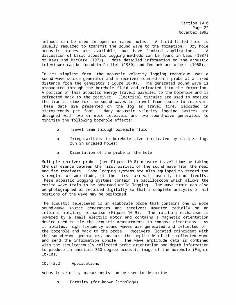
Section 10.0Page 23
November 1993
o Porosity (for known lithology)
o Lithology (determined in conjunction with other logs)
o Rock strength
o Fracture location
o Validity of seismic refraction interpretations
Porosity can be determined from the acoustic velocity log if the formation compensation is known and is clay-free, consolidated (grains cemented together) and fluid-bearing. The porosity is calculated from the relationship established by Wyllie (1963) which involves transit times through the rock and the pore fluids.
The accuracy of the calculated porosity is dependent on the accuracy of the matrix identification. Because the acoustic travel time varies with porosity and rock composition it is a non-unique response. Lithology can only be confirmed if other logs such as the neutron, gamma-gamma or natural gamma are used for verification. The acoustic travel-time log can be used to verify seismic model layers determined by the seismic refraction method (Section 3.0).
Matrix travel times for sedimentary rocks (shale, sandstone and limestone) are well documented and vary within known limits. Matrix travel times for igneous and metamorphic rocks vary considerably and are not well defined by the present literature. For this reason it is recommended that the interpretation of the acoustic velocity log be limited to identification of relative changes in porosity in igneous and metamorphic rocks, unless detailed information concerning rock type or seismic velocities are available. Dobrin (1976) provides a table of velocities for various sedimentary, igneous and metamorphic rocks (Table 10-2).
Relative rock strength can be estimated from acoustic travel-time data in zones of similar rock type. Increases in travel-time can indicate zones of weathering, alteration or fractures, which also have higher porosity than rock outside such zones.
The acoustic amplitude log can be used as an indication of conditions at the edge of the borehole, such as cement bonding quality between steel casing and the formation. If there is a good bond, the acoustic amplitude is high. However, if there is a gap caused by partial grouting, the signal from the formation will be weak (attenuated) and show as a low-amplitude zone. Low amplitude can also be an indication of fractures, unconsolidated or soft material, weathering, or mineral alteration in uncased holes.
The full waveform acoustic log records the complete acoustic wave so that various components of the wave may be identified. These components include the arrival times and amplitudes of:

Section 10.0Page 24
November 1993
o Compressional waves
o Shear waves
o Tube waves
Shear- and tube-wave data can be used to locate fractures and estimate permeability. The shear-wave and tube-wave information also is used to calculate engineering properties used in the design of remedial structures or systems. These engineering properties are:
o Bulk modulus
o Shear modulus
o Poisson's ratio
o Young's modulus
The reader is referred to Dobrin (1976) for a complete discussion of the calculation of these properties from seismic and acoustic log data.
The acoustic televiewer is used primarily to identify and measure the strike and dip of fractures. However, it can also be used to identify other borehole and rock conditions such as hole enlargements, hole obstructions, rock breakouts, foliation, and zones of weakness due to weathering or alteration.
10.4-2.3 Equipment
Acoustic logging methods require relatively complex electronic systems and instrument controls to produce acoustic logs. Sophisticated timing and measuring circuits are used to pulse the sound-wave generators and turn the receivers on and off. An oscilloscope is used to visually inspect the quality of the sound wave as it is transmitted and received. All of these components are contained in the surface electronics package. The probe contains the sound-wave generators and receivers. A specially designed camera may be necessary to record the full waveform acoustic log.
10.4-2.4 Field Procedures
The acoustic televiewer logs must be run at very slow probe speeds, commonly four feet per minute. Calibration of acoustic surface electronics is generally performed internally by passing a reference signal through the circuits. There are no calibrations needed for acoustic probe electronics apart from the surface system calibration. For quantitative velocity determination, it is best to calibrate the system by correlation with velocities determined by core tests or a seismic refraction survey.
10.4-2.5 Interpretation
Section 10.0Page 25
November 1993
The porosity value calculated from the acoustic velocity log represents the primary (intergranular) porosity only. Secondary porosity created by vugs, dissolution, and fractures is not detected by the acoustic velocity method because the sound wave travels along the fastest path, which is through the rock rather than the fluid. If the total porosity from the density or neutron log is compared to the primary porosity from the acoustic velocity log, the amount of porosity due to vugs and fractures can be determined.
When the amplitude of the received sound wave is low due to inhomogeneities in the rock (fractures, vugs), the first arrival of the sound wave may not be detected because it is below the detection limit of the probe. Later arrivals with higher amplitudes trigger the detector and show as very long travel time on the log. This phenomenon is called "cycle skipping." The log usually looks very spikey and irregular when cycle skipping occurs. Cycle skipping may indicate vugs, fractures or weak rock.
Acoustic travel times for specific depths can be plotted against gamma-gamma, neutron, or natural gamma count rates at corresponding depths to define rock-type groups (Figure 10-11). This technique, called cross-plotting, is very informative, especially when combined with core or other geologic data.
Full acoustic waveform interpretation is similar to vertical seismic profiling (VSP) interpretation; therefore the reader is referred to Section 10.4-4 for a more complete discussion.
Interpretation of acoustic televiewer images (logs) is somewhat subjective unless borehole wall character is evidenced on other logs. The basic premise is that strong signals from smooth borehole walls of competent rock appear as bright areas on the log, whereas fractures, soft seams and weathered rock appear as dark areas.
10.4-2.6 Advantages and Disadvantages
The acoustic probes are advantageous because they provide perhaps the most accurate information concerning fracture location, geometry and characterization, and need not require confirmation by other log types for some purposes.
The primary disadvantage of acoustic velocity techniques is their relatively high cost and complexity, and their limited value in cased holes penetrating unconsolidated materials. The acoustic tools must be run in water-filled holes so that the sound wave is effectively transmitted to the borehole walls. However, special receivers are available for use in dry holes, but they must be clamped to the side of the borehole, thus preventing continuous logging of the hole.
The acoustic televiewer is not readily available among geophysical contractors, because it is an expensive, relatively specialized probe. Furthermore, the quality of the log, and thus reliability of interpretation, depends strongly on the operator's experience and ability
Section 10.0Page 26
November 1993
to set the proper acoustic focus. As major changes in the borehole diameter occur, refocusing is commonly required.
The reader is referred to Zemanec and others (1969 and 1970) or Taylor (1983) for a complete discussion of the interpretation of the technique. 10.4-3 Nuclear (Radiation) Methods
10.4-3.1 Principles of Operation
Nuclear logging methods include both passive (natural gamma-ray) and active (gamma-gamma and neutron) techniques. These techniques are used primarily for the determination of porosity and lithology. Most nuclear methods employ the use of geiger tubes or scintillation crystals to detect the intensity of radioactivity. The detector emits photons (flashes of light) when struck by radioactive particles (neutrons and gamma-rays). The photons are converted to electrical pulses and sent uphole to counting and timing circuits, where a surface electronics module converts these pulses into counts per second. All nuclear logs can be run in open or cased holes, and in dry or water-filled holes.
10.4-3.1.1 Natural Gamma-ray Log
The natural gamma-ray log is a measure of the naturally-occurring gamma radiation in the formation. Natural gamma radiation is produced by the radioactive decay of potassium, thorium (Th) and uranium (U) atoms. Clay minerals show high gamma ray readings because they commonly contain potassium in their chemical structure. Clay minerals also promote the adsorption of positive ions, such as Th+ and U+, because of their open crystal lattice structure and net negative charges. Thus, the natural gamma log serves as a reliable clay indicator in those environments where non-clay beds do not contain radioactive minerals. However, some granites and their weathering products are also rich in radioactive minerals, and also will give high gamma-ray counts.
10.4-3.1.2 Gamma-gamma Log
Gamma-gamma logging uses a solid, encapsulated radioactive source (generally cesium-137 or cobalt-60) mounted 10 to 35 inches from the detector to bombard the formation with medium-energy gamma-rays. The gamma-rays are scattered as they collide with the electrons of the material in the formation. With each collision, an individual gamma particle will lose some of its energy until it reaches a low energy state and is absorbed by an electron. The probe measures the number of gamma rays that are reflected back to the detector. The number of electrons detected by the instrument is inversely proportional to the density of the formation evaluated. Therefore, very dense formations, which have high electron densities and will reduce gamma energy quickly, will cause fewer gamma rays to reach the detector, while less dense formations will exhibit higher gamma count rates. If the formation lithology (and density) are known, variations of density measured can be attributed to changes in porosity.
10.4-3.1.3 Neutron-epithermal-neutron Log
Section 10.0Page 27
November 1993
The neutron-epithermal-neutron log is used to determine porosity as a function of formation hydrogen content. The basic assumption in the calculation of porosity using this method is that all pore (void) spaces in a formation are water filled. This survey method can be employed below the water table to measure porosity and above the water table to indicate relative moisture content in the unsaturated zone.
The neutron probe is similar in design to the gamma-gamma probe, except an americium-241 beryllium radioactive source is installed. This source emits fast neutrons which collide with atoms in the formation and are slowed down. The most effective atom in slowing down fast neutrons (because of its similar atomic mass) is the hydrogen atom, which is a major constituent of water. When neutrons reach a very low energy level they are captured primarily by hydrogen atoms, and gamma energy is released. Detectors are designed to detect (count) either neutrons or gamma photons released by neutron collisions. The counting rate for both types of detectors is inversely proportional to the hydrogen content of the formation. The instrument detection results are converted to porosity.
Although a neutron log cannot be used for measuring porosity above the water table, it is very useful for measuring changes in the moisture content.
10.4-3.2 Applications
Nuclear techniques are used primarily to identify the presence of clay, correlate lithologies, and determine porosity. These techniques are most valuable if the probes are calibrated with appropriately-constructed field standards of known properties, and, therefore, accurate densities and porosities can be determined. The gamma-gamma and neutron radiation logs provide a record of count rate, which must be scaled with a calibration rating curve after dead-time corrections are applied (moderate to high count rates only) to provide porosity values.
Natural gamma and neutron logs can aid in the identification of perched aquifers, especially when used with a resistivity technique. Opposite a perched aquifer the resistivity is low; the neutron log would show increased water content, and the natural gamma should confirm the perched zone to be non-clayey materials. As the resistivity and neutron probe responses may be similar for clay and water-saturated sands due to water molecules bound to the structure of clay minerals, the natural gamma log is critical for correct interpretation.
10.4-3.3 Equipment
The three nuclear techniques use very similar surface and downhole equipment. While a few nuclear logging systems use the same probe and detector for all three methods, with only the source and source-to-detector spacings changed, most logging systems employ the same probe for natural gamma and gamma-gamma, but a different probe for neutron. The uphole electronics consists of a counting and timing circuit for
Section 10.0Page 28
November 1993
recording data in counts per second. A more complex electronics package is required for directly recording porosity during gamma-gamma or neutron logging.
The gamma-gamma and neutron methods require the use of a solid, encapsulated, chemical radioactive source. Although these sources are relatively small, they present a safety concern for the operators of the equipment. The sources are regulated by the Nuclear Regulatory Commission (NRC) and must be licensed. Use of licensed sources is limited to those persons who have proper training and have obtained NRC certification in nuclear materials handling and safety. These sources are transported and stored in locked, shielded carrying cases and are secured to the probe only during actual logging.
Another aspect of safety is the use of active sources in uncased, loose formations. The potential for getting a probe stuck in the hole often is significant when borehole walls consisting of unconsolidated soils are unstable. It is recommended that no probe with a radioactive source be run in an uncased hole in an unconsolidated formation.
10.4-3.4 Field Procedures.
Nuclear logging methods follow the same general field procedures as other logs. One notable difference is that radioactive sources used with the density and neutron techniques are installed using a site-specific field routine that minimizes radiation doses to the operator. Also, log quality and repeatability are enhanced if a probe decentralizer is used in hole diameters of 8 inches or greater. Probes are calibrated at the site using either a source of known strength (field standard) to check detector response or a piece of material with known physical properties to check total probe response.
For uncased holes in competent rock, a caliper probe is always run before the nuclear probes because of the serious consequences of getting a radioactive source stuck in the hole.
Radiation probes are generally run at a slower speed (10-15 ft/min) than most other probes so that the count rates can be averaged over a longer period of time, thus reducing the statistical variability and making the logs more repeatable.
10.4-3.5 Interpretation
None of the radiation logs have a unique count rate response to individual lithologies (see Figure 10-12); however, within a single geohydrologic environment, any given geohydrologic unit (layer) generally shows a consistent response. This aspect gives these logs much value in correlating lithology between well sites.
Natural gamma logs respond primarily to the amount of potassium, and secondarily to the amount of thorium and uranium isotopes in the formation. As potassium is a major component of most clay minerals, the
Section 10.0Page 29
November 1993
natural gamma log is generally considered to be a clay-content log. Other minerals that can cause high gamma counts include:
o Feldspars (high potassium) - found in many granites and other light-colored igneous and metamorphic rocks
o Micas (high potassium; may contain thorium) - found in granites
o Hornblende (can contain thorium and uranium) - a common accessory mineral in granites and some metamorphic rocks
o Uranium minerals in granites and sands
Sometimes, a natural gamma log will show high radioactivity opposite fractures or fractured zones in bedrock. These spikes are usually due to uranium-rich mineral precipitates lining the fracture walls, but small excursions on the log may represent clay-filled fractures.
Natural gamma log responses should be cross-examined with the SP and one of the resistivity log types to confirm rock type. Fractures can usually be identified with the single-point resistance log.
Neutron logs will respond to water bound in the crystal structure as if it were pore water. It is important to check for the presence of clay with SP or natural gamma when using the neutron log to determine porosity. The neutron probe is affected by borehole enlargements and high chloride content. Under these conditions, the neutron log should be used only as a general indicator of porous zones.
Rocks and glacial sediments show an extremely wide range of bulk densities (the combined density of rock, fluid, and air). If the lithology is known, a reasonable estimate of porosity can be made by using published relationships.
The density log can also be used to detect voids and channeling in grout behind casing. Voids and channels in grout may provide pathways for transport of water and contaminants between layers.
When analyzed together, the gamma-gamma and neutron logs commonly indicate zones of formation washout that exist behind the well casing, caused by the drilling process. Washouts and aquifers may give a similar response on these logs, and commonly the natural gamma log must be consulted.
10.4-3.6 Advantages and Disadvantages
Nuclear techniques work well in a wide variety of borehole environments including cased (PVC or steel) and uncased holes in saturated and unsaturated formations. Their primary advantage is that, when properly calibrated, these logs give estimates of porosity and lithology that are consistent with independent field and laboratory test results. The porosity and lithology measurements are made in-situ at accurately known
Section 10.0Page 30
November 1993
depths, thus reducing cost and time involved in comparison to core sampling and aquifer test pumping.
Most of the probe response in nuclear logging is from the first six inches to one foot of the formation surrounding the borehole. Sometimes this zone may be very disturbed, due to drilling and completion procedures that may force drilling fluids into pore spaces near the borehole or alter the compaction of loose materials. If large augers are used and a small diameter well is installed, most of the radiation response is from the gravel pack (filter sand) or backfilled material. In such cases a false indication of formation properties may be obtained. The best hole conditions result from driving casing or open-hole drilling in competent rock.
Hole diameter variation and rugosity of the borehole walls affect all nuclear logs to some degree, depending on source strength and the chosen spacing between source and detector. Gamma-gamma density logs made with a weak radiation source and short spacing may be severely affected, misrepresenting true formation density. Neutron probes have a lesser sensitivity to the same conditions, while natural gamma logs generally are not significantly affected unless a large void or washout is present. Caliper logging in open holes provides data for correcting radiation logs for hole diameter variations. However, quantitative determination of density and porosity opposite washouts in cased wells is not possible.
Radioactive sources are regulated by the NRC and must be licensed. The use of geophysics tools employing radioactive sources is restricted to only those persons who have NRC certification. The consequences of losing a radioactive source (i.e., by being unable to retrieve a downhole source/probe) is serious and costly.
10.4-4 Vertical Seismic Profiling (VSP)
10.4-4.1 Principles of Operation
Vertical Seismic Profiling (VSP) is a borehole seismic survey method used to detect and characterize open fractures within rock. The VSP method was developed in the petroleum industry and has recently been applied to hydrogeologic characterization for environmental studies. This method provides a three-dimensional image of subsurface velocities and geologic structure, utilizing an array of seismic borehole geophones (motion sensitive sensors) or hydrophones (pressure sensitive sensors) placed in a borehole at the depths of interest. The technique is illustrated schematically in Figure 10-13.
The VSP technique uses a seismic source, placed at the surface some distance away from the borehole to generate seismic waves, which travel through the ground and are detected by the geophones in the borehole. These waves consist of compressional waves (P waves) and shear waves (S waves). Figure 10-13 shows a schematic representation of the seismic wave received by the geophones.
When a fluid-filled fracture, which intersects the borehole, is squeezed
Section 10.0Page 31
November 1993
by compression from a seismic wave, a pressure pulse known as a tube wave is generated in the borehole. The tube wave is detected by the geophones as the pressure pulse is propagated upward and downward in the borehole. The size (amplitude) of tube waves generated by a permeable fracture depends on the hydraulic conductivity of the fracture, elastic properties of the rock, fluid properties, and borehole radius. High permeability fractures yield large amplitude tube waves. Tube wave amplitudes are generally much larger than those of compressional waves (see Figure 10-13).
10.4-4.2 Applications
A particular application of this technique is the detection of open, water-filled fractures which are intersected by a borehole (Levine and others, 1985). Compressional, shear, and tube waves can be used to characterize the fractures in terms of depth, attitude, and hydraulic conductivity.
When the formation and fluid properties are known, tube wave amplitudes can be used to determine the hydraulic conductivity (K) of a fracture. The K value is determined through the comparison of compressional wave pressure amplitude to that of the tube wave as measured by the hydrophone positioned closest to the fracture depth. The use of the nearest hydrophone removes the effects of the source as well as the recording system response.
If desired, the lateral extent of the fracture can be delineated by moving the surface source away from the borehole and observing changes in the transmitted and reflected compressional and shear waves (see Figure 10-14). Because the compressional and shear waves scatter, attenuate, reflect, and refract at a fracture zone, computer ray-tracing methods can be used to image the geometry of the fracture. Of particular note is the significant attenuation of shear wave energy through a fracture zone or other low velocity zone.
10.4-4.3 Equipment
A string of hydrophones or unclamped geophones are used in the borehole to detect the tube waves. The hydrophone responses are transmitted to a surface recording unit. This surface unit should consist of digital recording instrumentation capable of timing in the range of tens of microseconds and with playback capability for later analyses.
The VSP technique generally uses conventional seismic sources (e.g., weight drop, explosives, Betsy seisgun) placed on the ground surface at appropriate locations or within nearby shallow borings. The energy source with the highest frequency content consistent with the attenuation characteristics of the earth materials at that location should be used.
10.4-4.4 Field Procedures
Section 10.0Page 32
November 1993
The following field procedures allow fracture characteristics, primarily depth, length, and orientation, to be determined.
Surface energy sources are arranged in a radial pattern around the hole and placed at various distances from the borehole. Receivers are placed within the uncased bedrock segment of the borehole. Each source location is detonated individually, with data being stored digitally for each geophone for each shot. After all seismic recordings are made, the sensor array may be raised or lowered in the borehole to span deeper or shallower unmonitored segments. Sensor spacings are directly related to the degree of accuracy with which individual fractures or fracture zones need to be defined. Wide sensor spacings (25 to 50 feet) are useful in identifying depths to zones of fractures; closer sensor spacings (5 to 10 feet) may identify individual fractures. Additional data are recorded until the entire water-filled section of the borehole has been surveyed. The data are stored on magnetic tape or disk for further computer processing, such as amplitude, frequency and particle motion analysis. A complete display of VSP data from the top to the bottom of a borehole can also be made using the stored data.
10.4-4.5 Interpretation
Tube waves indicative of permeable fracture zones are often readily apparent on the seismic recordings. By using an appropriate X-Y data display (individual sensor seismograms with time along one axis and depth along the other axis), the depth at which the tube waves originate can be determined within a few feet if closely-spaced sensors are employed. The orientation of the fracture can be approximated by analysis of the tube-wave to compressional-wave amplitude ratio. Geophone records from energy sources located at the same distance, but different angles, around the borehole are used for this analysis. Because of the qualitative nature of the analysis, results are presented in terms of shallow-, moderately-, or steeply-dipping fractures. Analysis of the amplitude ratios will define the strike of steeply-dipping fractures to within ±10 degrees, and that of moderately-dipping fractures to within ±15 to 20 degrees. The more data available from different azimuths, the better is the fracture orientation definition.
The continuity and extent of fractures can best be determined if multiple boreholes are investigated. If a fracture intersects two boreholes, the continuity of the fracture can be determined through computer modeling and imaging. Borehole-to-borehole seismic methods can also be used to establish fracture continuity through the use of guided wave technology (i.e., energy generated in the vicinity of permeable fractures in one borehole and high-amplitude, high-frequency seismic waves recorded in an adjacent borehole).
The tube-wave amplitude is generally influenced by the hydraulic conductivity of the fracture. Other factors such as the physical properties of the medium surrounding the borehole, the frequency of the seismic waves, the properties of the fluid filling the borehole, and the radius of the borehole may also affect the amplitude. The amplitude ratio (tube-wave to P-wave) versus frequency is the key relationship used
Section 10.0Page 33
November 1993
to establish the hydraulic conductivity of a fracture zone. A set of curves can be generated showing amplitude ratio versus frequency for different hydraulic conductivity values. A set of such curves is shown on Figure 10-15. The determination of hydraulic conductivity values by the VSP technique has been verified through correlation with permeability test data.
10.4-4.6 Advantages and Disadvantages
Vertical seismic profiling yields clear and definitive results for identifying permeable fractures intersecting a borehole. As numerous studies have shown, some fractures detected by other logging techniques, such as acoustic logging, borehole televiewer, electrical and caliper logging, are not permeable and are not fluid conductive.
The VSP technique has been used in all types of rock with varying degrees of success. The greatest successes for fracture and hydraulic conductivity objectives have been achieved in igneous and competent metamorphic rocks, which appear to have rather distinctive faulting and fracturing zones. Its use in sedimentary rocks and weathered metamorphic rocks, which may have extensive zones of permeable materials, has been less successful.
VSP results away from the borehole are limited to the seismic-ray paths from the seismic source to the detectors. This procedure may, or may not, be sufficient to determine the lateral extent of a fracture away from the borehole and provide control on the attitude of any permeable fractures identified.
The VSP technique requires relatively sophisticated equipment when compared with many of the other borehole techniques. It is also time-consuming and, thus, relatively expensive.
10.5 GLOSSARY
Active technique - A technique in which a stress is applied to the material under study and the resultant response is measured. Stresses can include electrical current, sound waves, or neutron or gamma ray bombardment.
Calibration - The process wherein the zero and sensitivity of the logging circuitry is set so that the recorded measurements will be accurate with respect to industry-standard units of measurement for a specific log-type (i.e., grams/cubic centimeter for rock density).
Dead time - In radioactive logging, the length of time (usually measured in microseconds) required by a logging system to recover from counting one disintegration event in order to count (record) the next event. Events occurring during dead time are not counted.
Formal depth-registered log - A geophysical log recorded on graph paper or digitally in which accurate downhole depths are simultaneously and systematically registered opposite corresponding log responses, and
Section 10.0Page 34
November 1993
detailed logging run information is recorded in a log header.
Lithology - The physical character and composition of a rock, implying a specific rock or soil type.
Measuring point - The point, on a probe, where the reading is taken (e.g., the tips of the caliper arms; the detector on a gamma-ray probe).
Non-unique response - Response that is not unique to a specific rock characteristic. As examples, several different rock types exhibit low gamma-ray counts; or water-filled fractures and clay layers both have low resistivity values.
Passive techniques - A technique which measures properties inherent to the material. Examples include SP, gamma-ray, temperature.
Probe - The downhole electronics and detecting/measuring apparatus of the logging system, usually encased in a stainless steel jacket.
Radioactive decay - The transformation of an unstable isotope into an isotope of another element, resulting in a loss of energy and the emission of radiation (e.g., alpha or beta particles, neutrons and/or gamma rays). Reference elevation - The aboveground elevation which is designated as a common point for referencing all measurements for correlative purposes (commonly, ground surface or top of casing).
Resolution (vertical) - The capability of a logging system to distinguish geophysical changes between closely spaced (thin) lithologic units.
Rugosity - The degree of roughness or irregularity of the borehole wall, which affects some log types.
Total depth (TD) - The deepest point in the boring as determined by accurate measurement, in this instance geophysical logs. Discrepancies commonly occur between total drilling depth and total depth from geophysical logs, due to filling of the bottom of the borehole from caved material or to cable stretch (very deep holes only).
Section 10.0Page 35
November 1993
REFERENCES
Clark, Jr., S.P., (ed.), 1966, Handbook of physical constants, rev. ed., Geological Society Am. Rem. 97.
Collier, H.A., and Alger R.P., 1988, Recommendations for obtaining valid data from borehole geophysical logs: in Proceedings of the
Second National Outdoor Action Conference on Aquifer Restoration, Groundwater Monitoring, and Geophysical Methods, Vol. 2, presented by the Association of Groundwater Scientists and Engineers (AGSE) and U.S. EPA EMSL, Las Vegas, Nevada, May 23-26, 1988, pp. 897-923.
Commonwealth of Massachusetts; Department of Environmental Protection,Standard References for Monitoring Wells, Publication Number WSC 310-91.
Conaway, John, 1987, Temperature logging as an aid to understanding groundwater flow in boreholes: in Proceedings of the Second International Symposium on Borehole Geophysics for Minerals, Geotechnical, and Groundwater Applications, published by the Minerals and Geotechnical Logging Society, a Chapter-at-Large of the Society of Professional Well Log Analysts, Houston, Texas, pp. 51-59.
Davison, C.C., Keys, W.S., and Paillet, F.L., 1982, Use of borehole-geophysical logs and hydrologic tests to characterize crystalline rock for nuclear-waste storage, Whiteshell Nuclear Research Establishment, Manitoba, and Chalk River Nuclear Laboratory, Ontario, Canada: Office of Nuclear Waste Isolation ONWI-418, NTIS, Springfield, VA, 103 p.
Dobrin, M.B., 1976, Introduction to geophysical prospecting, 3rd ed.: New York, NY, McGraw-Hill, 630 p.
Driscoll, F.G., 1986, Groundwater and wells: St. Paul, Minnesota, Johnson Division, UOP, 1089p.
Hess, A.E., 1982, A heat-pump flowmeter for measuring low velocities in boreholes: U.S. Geological Survey Open-File Report. 82-699, 40 p.
____, 1985, Identifying hydraulically-conductive fractures with a low-velocity borehole flowmeter: Canadian Geotechnical Journal, v. 23, no. 1, pp. 69-78.
Hilchie, D.W., 1978, Applied open-hole log interpretation: Golden, CO, D.W. Hilchie, Inc.
Keys, W.S., and MacCary, L.M., 1971, Application of borehole geophysics to water-resources investigations: U.S. Geological Survey, Techniques of Water-resources Investigations, Book 2, Chapter E1, 126 p.
Kwader, Thomas, 1982, Interpretation of borehole geophysical logs in shallow carbonate environments and their application to groundwater
Section 10.0Page 36
November 1993
resource investigations: Tallahassee, FL, Florida State University, unpublished Ph.D. dissertation, 332 p.
Labo, J., 1987, A practical introduction to borehole geophysics - an overview of wireline well logging principles for geophysicists: Tulsa, Oklahoma, Society of Exploration Geophysicists, 330 p.
Levine, E.N., Cybriwsky, Z.A., and Toksoz, M.N., 1985, Detection of permeable rock fractures and estimation of hydraulic conductivity by 3-D vertical seismic profiling: in Proceedings of the NWWA/EPA Conference on Surface and Borehole Geophysical Methods in Groundwater Investigations, National Water Well Association, Dublin, Ohio, pp. 853-876.
Paillet, F.L., 1980, Acoustic propagation in the vicinity of fractures which intersect a fluid-filled borehole: Society of Professional Well Log Analysts' Transactions, 21st Annual Logging Symposium, Lafayette, LA, p. DD1-DD33.
Patten, E.P., and Bennett, G.D., 1962, Methods of flow measurement in well bores: U.S. Geological Survey Water-supply Paper 1544-C, 28 p.
Schimschal, Ulrich, 1981, Flowmeter analysis at Raft River, Idaho: Groundwater, v. 19, no. 1, pp. 93-97.
Society of Professional Well Log Analysts (SPWLA), 1984, Glossary of terms and expressions used in well logging, 2nd ed.: Houston, TX, Society of Professional Well Log Analysts, Ransom, R.C., ed. and compiler, 116 p.
Taylor, T.J., 1983, Interpretation and application of borehole televiewer surveys: in 24th Annual Logging Symposium Transactions,
Houston, Society of Professional Well Log Analysts, Paper QQ, 19 p.
Tsang, C.F., 1987, A borehole fluid conductivity logging method for determination of fracture inflow parameters: Berkeley, CA, Lawrence Berkeley Laboratory, LBL-23096, NDC-1, 53 p.
Wyllie, M.R.J., 1963, The fundamentals of well log interpretation: New York, NY, Academic Press, 238 p.
Zemanek, J., Caldwell, R.L., Glenn, E.E., Jr., Holcomb, S.W., Norton, L.J., and Straus, A.J.D., 1969, The borehole televiewer - a new logging concept for fracture location and other types of borehole inspection: Dallas, Texas, Society of Petroleum Engineers, 43rd Annual Meeting (Houston) preprint SPE-2402; Journal of Petroleum Technology, v. 21, no. 6, pp. 762-774.
____, Glenn, E.E., Jr., Norton, L.J., and Caldwell, R.L., 1970, Formation evaluation by inspection with borehole televiewer: Geophysics, v. 35, pp. 254-269.
Section 10.0Page 37
November 1993

Section 10.0Page 38
November 1993
ADDITIONAL REFERENCES
Keys, W.S., 1988, Borehole geophysics applied to groundwater hydrology:Denver, CO, U.S. Geological Survey Books and Open-File Reports, Federal Center, Open-File Report 87-539.

Section 10.0Page 39
November 1993
SECTION 10.0BOREHOLE GEOPHYSICAL METHODS
LIST OF FIGURES
Figure Title Page No.
10-1 Typical Geophysical Logging Setup...............42
10-2 Caliper Probes.................................43
10-3 Interpretations of Borehole Temperature Profiles.......................................44
10-4 SP Log Example ................................45
10-5 Example of Flowmeter Log.......................46
10-6 Resistivity Probes ............................47
10-7 F Versus Φ Plot for Sandstones ................48
10-8 Acoustic Velocity Logging......................49
10-9 Acoustic Televiewer Diagram....................50
10-10 Example of Acoustic Televiewer Image............51
10-11 Example of Cross-plot of Acoustic Velocity and Neutron Logs with Geologic Interpretation.................................52
10-12 API Gamma Ray Units for Various Tertiary Sediments......................................53
10-13 Tube Waves Generated by Seismic Energy Incident or Permeable Fracture Zones............54
10-14 VSP to Determine 3D Geometry of Strata, Moduli Values and Permeability.................55
10-15 Relationship Between Hydraulic Conductivity and Ratios of Tube Waves to P Wave Amplitudes as a Function of Frequency.....................56
Section 10.0Page 40
November 1993
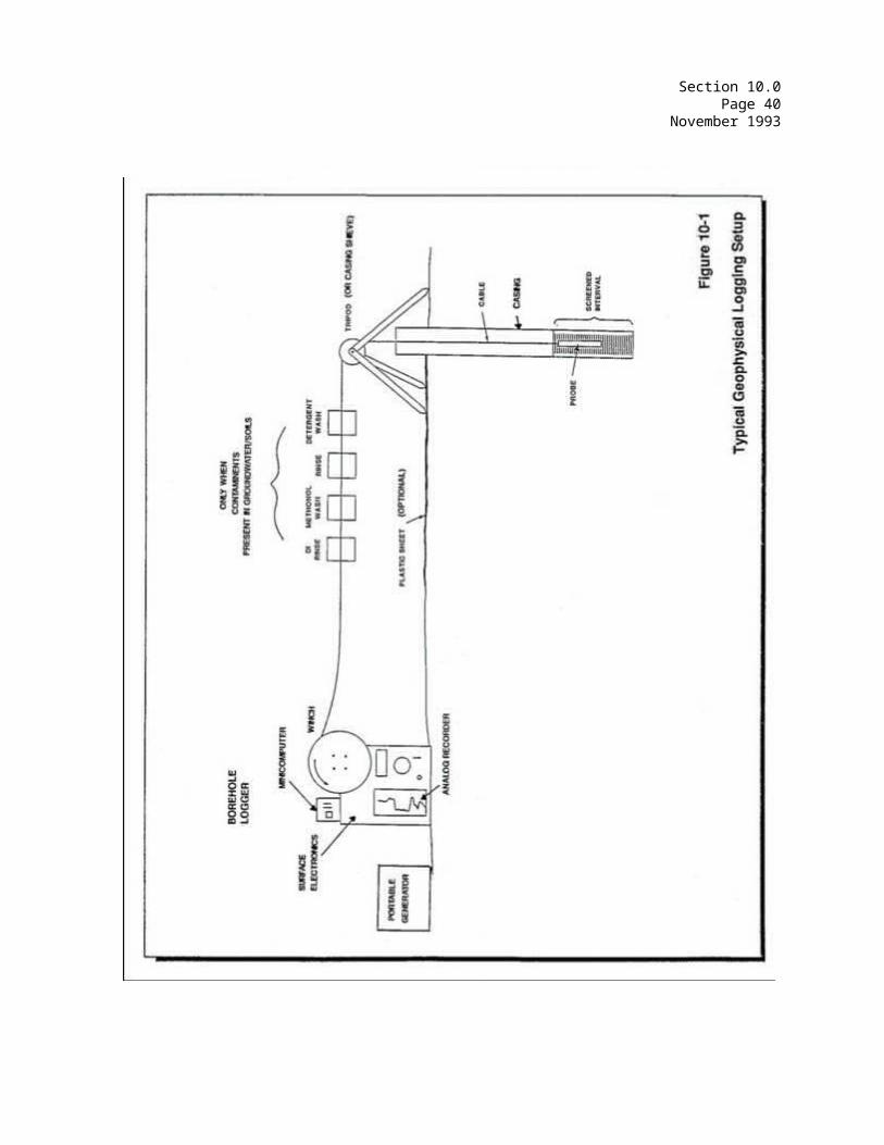
Section 10.0Page 41
November 1993
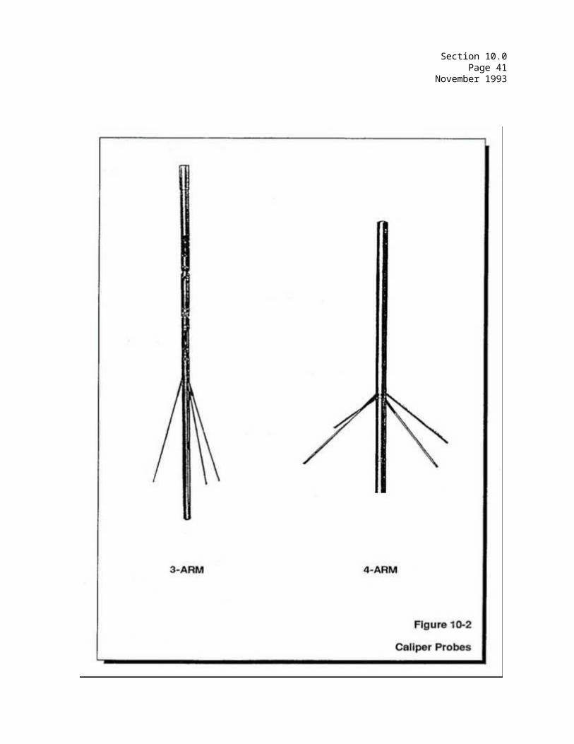
Section 10.0Page 42
November 1993
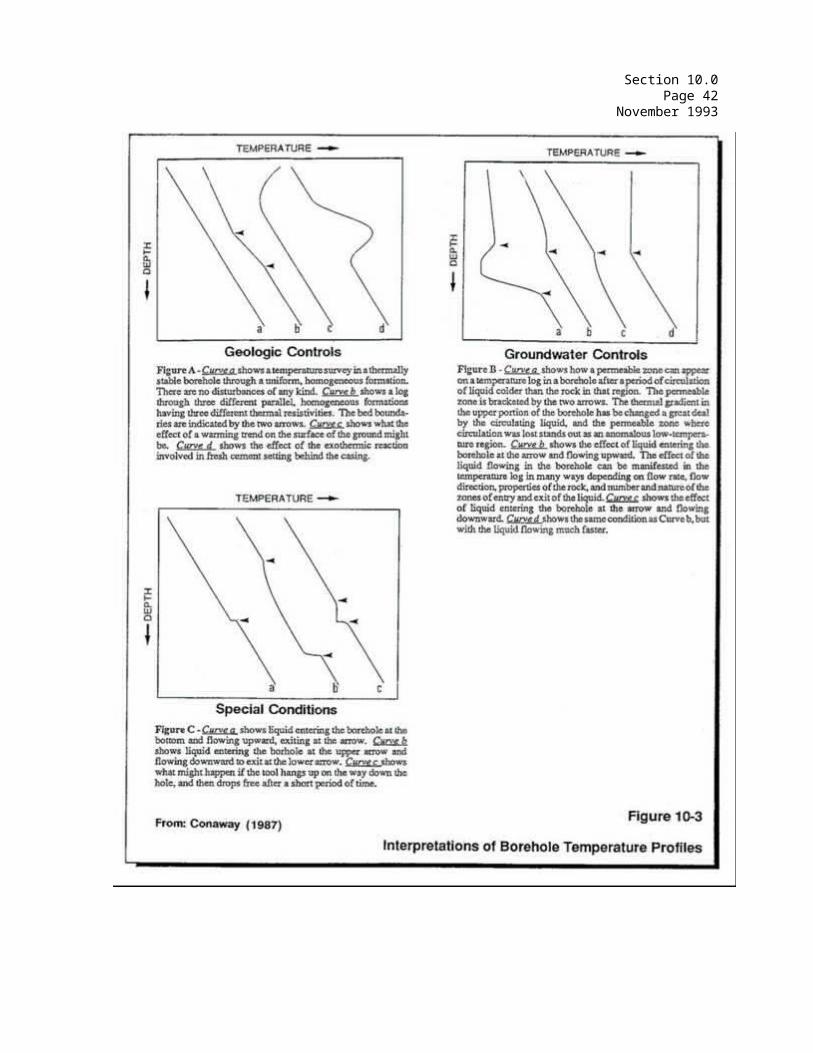
Section 10.0Page 43
November 1993
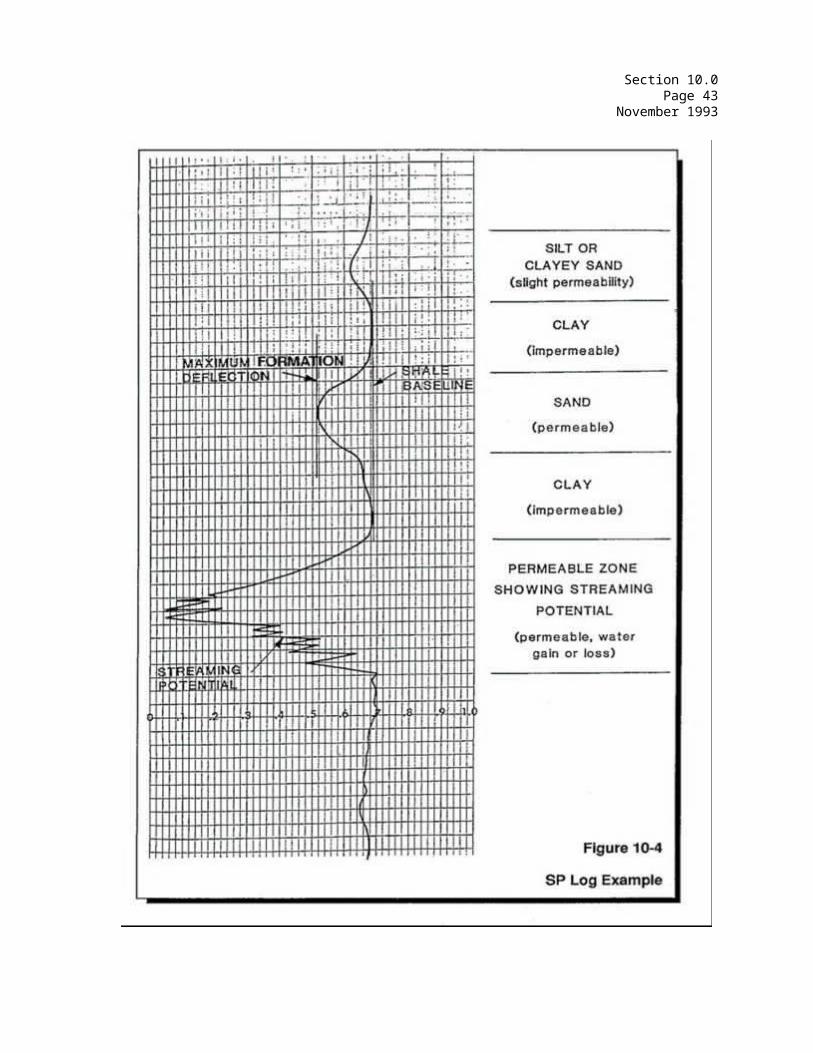
Section 10.0Page 44
November 1993
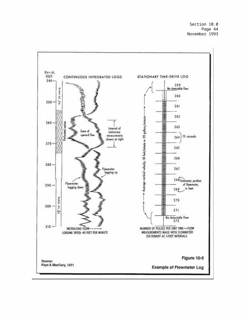
Section 10.0Page 45
November 1993
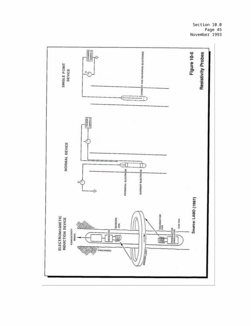
Section 10.0Page 46
November 1993
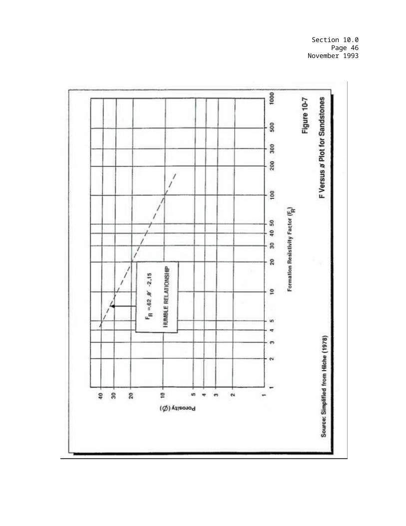
Section 10.0Page 47
November 1993
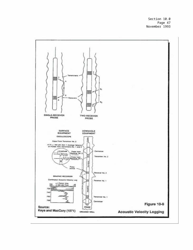
Section 10.0Page 48
November 1993
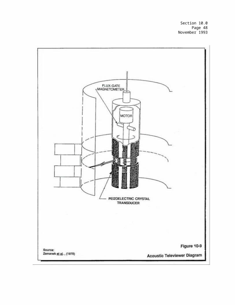
Section 10.0Page 49
November 1993
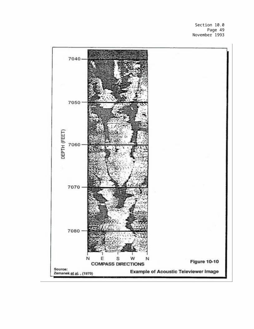
Section 10.0Page 50
November 1993
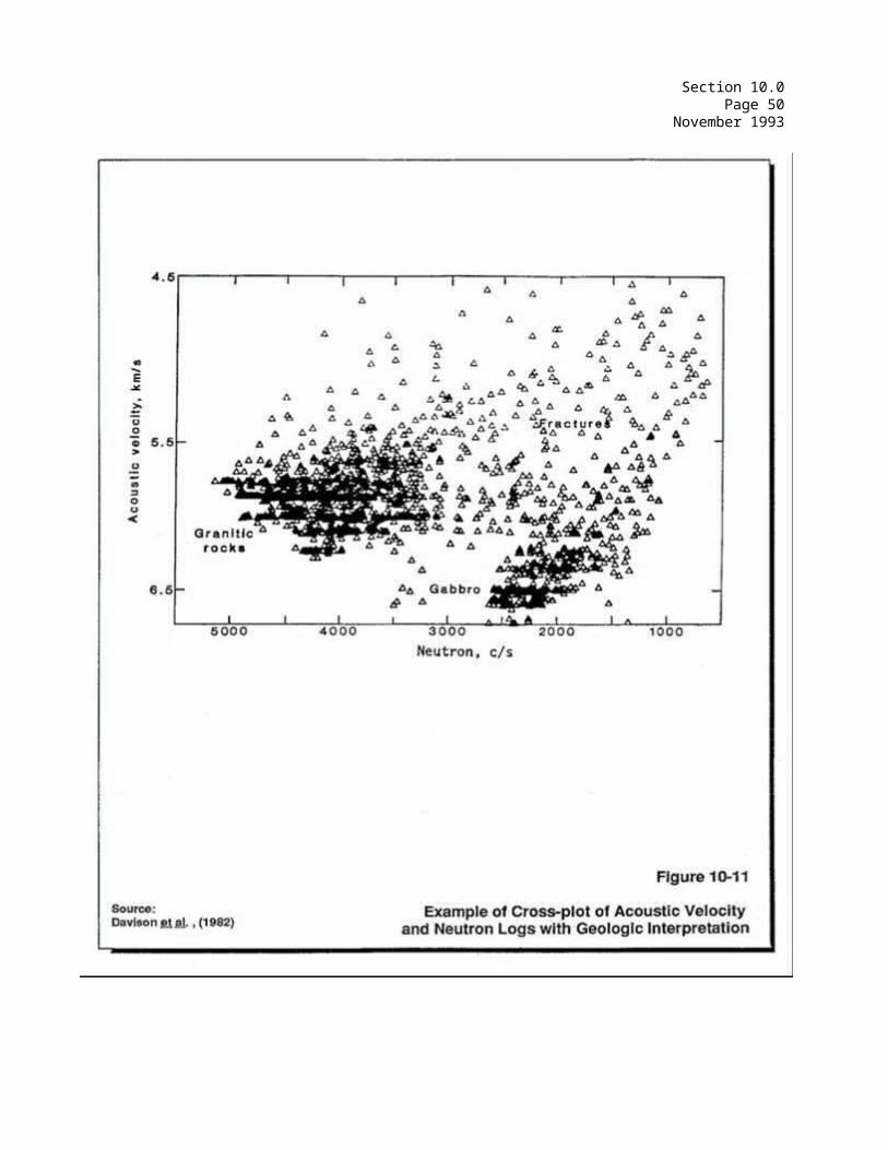
Section 10.0Page 51
November 1993
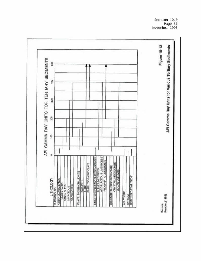
Section 10.0Page 52
November 1993
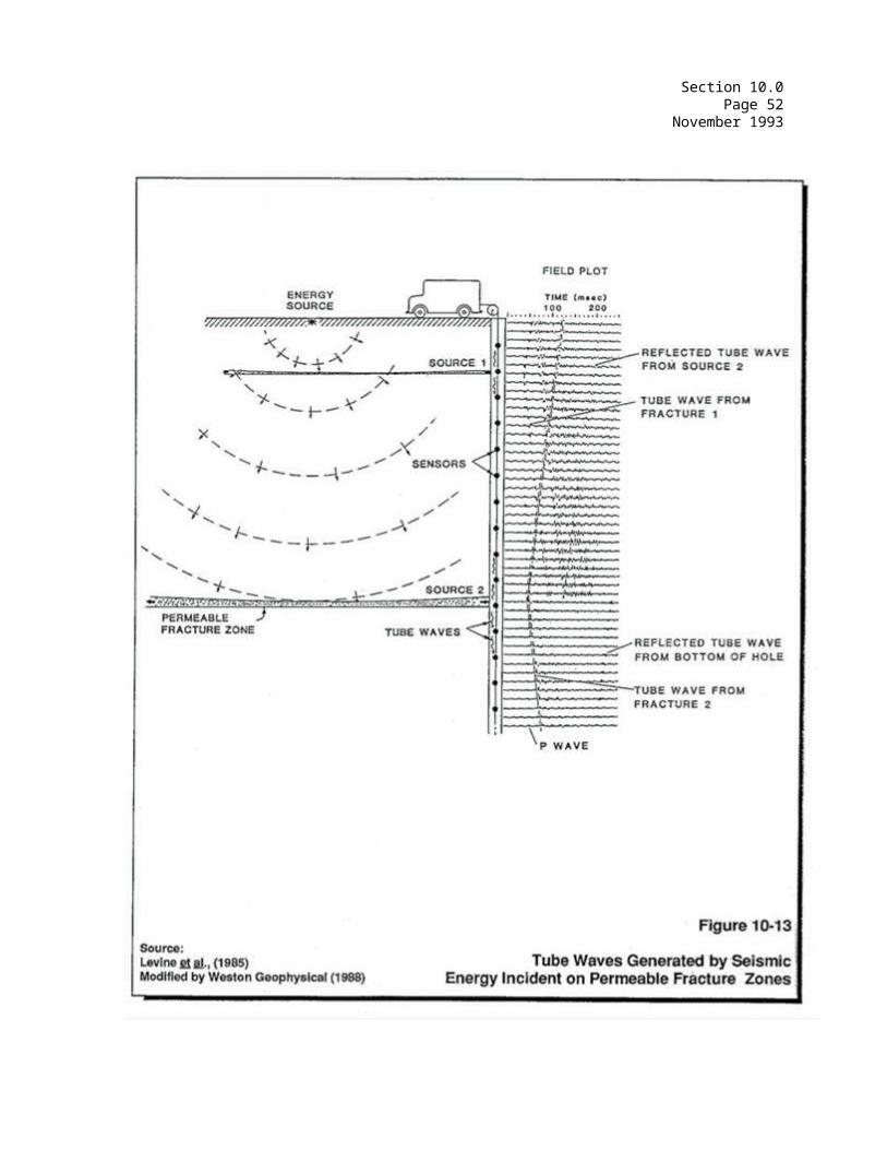
Section 10.0Page 53
November 1993
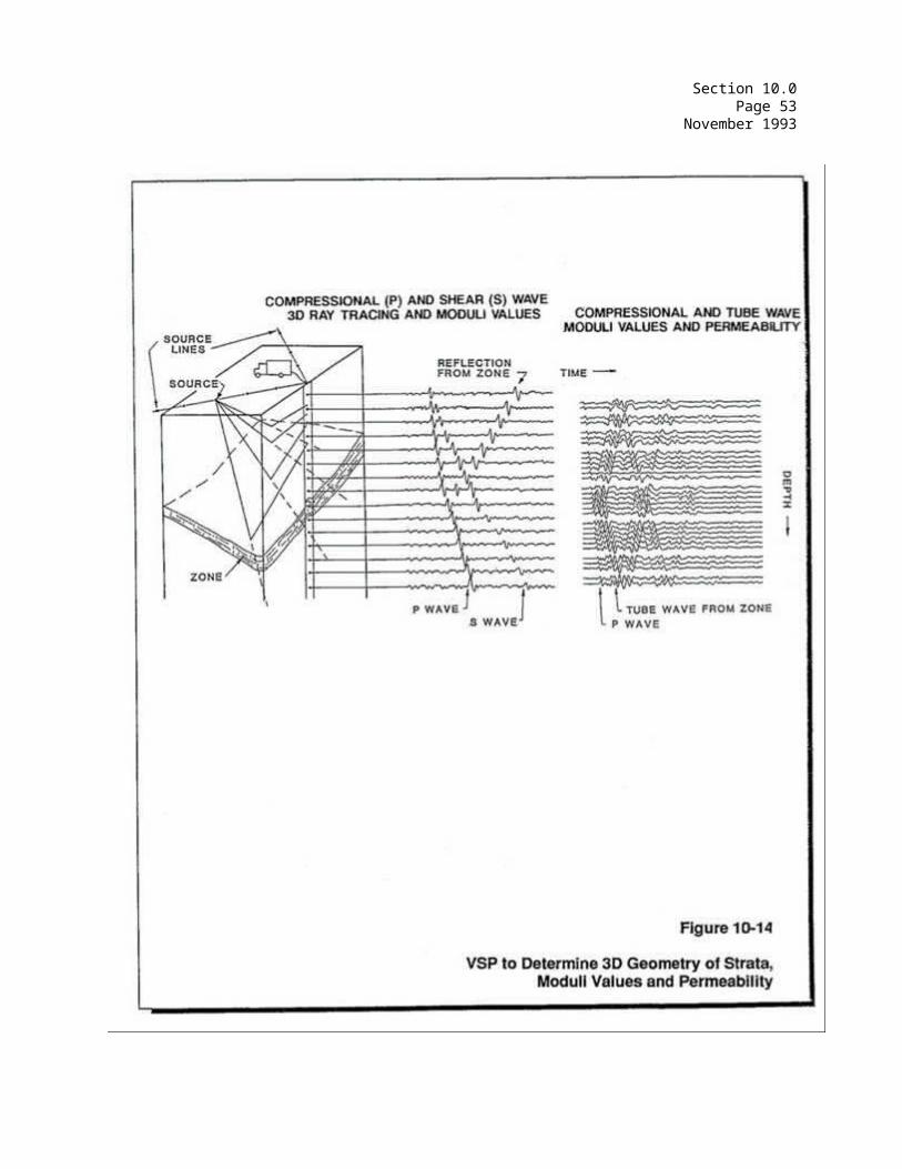
Section 10.0Page 54
November 1993
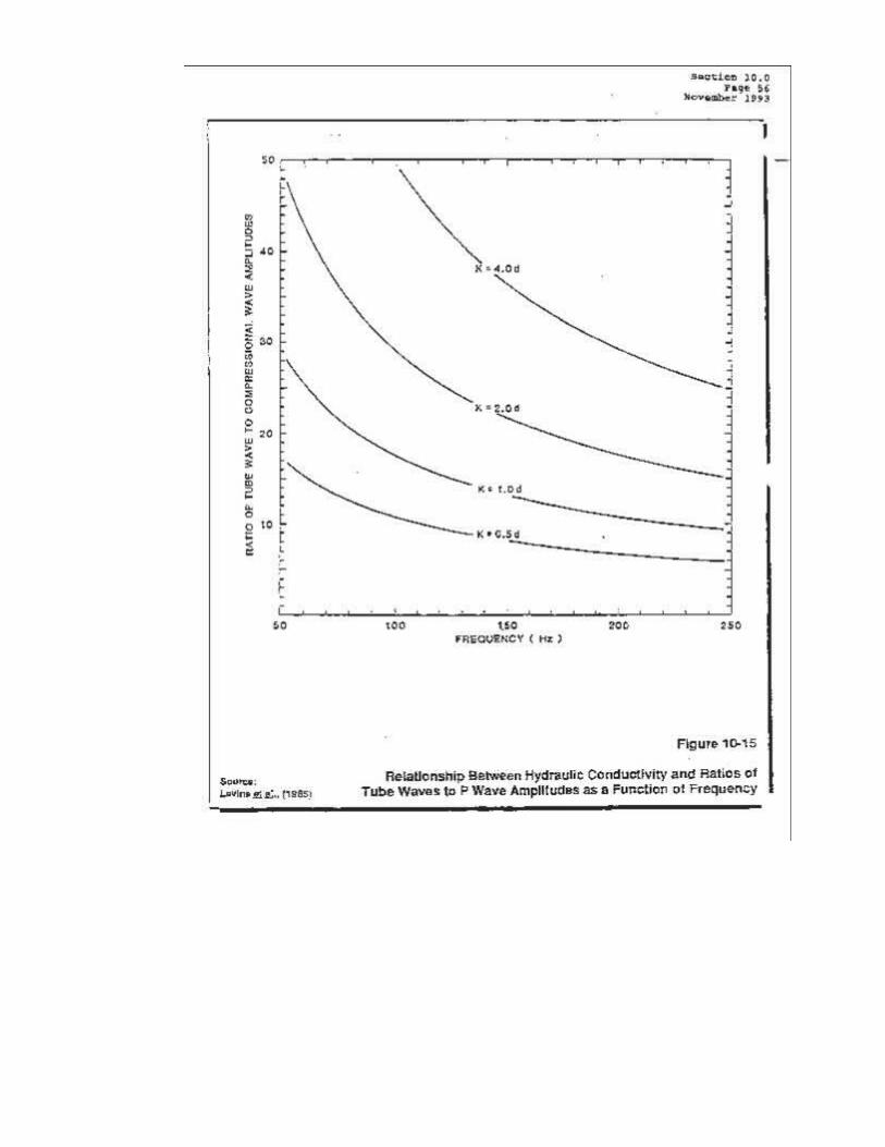
Section 10.0Page 55
November 1993
SECTION 10.0BOREHOLE GEOPHYSICAL METHODS
LIST OF TABLES
Table Title Page No.
10-1 Common Borehole Logging Techniques..............58
10-2 Compressional and Shear Velocities in Rocks.....59
Section 10.0Page 56
November 1993
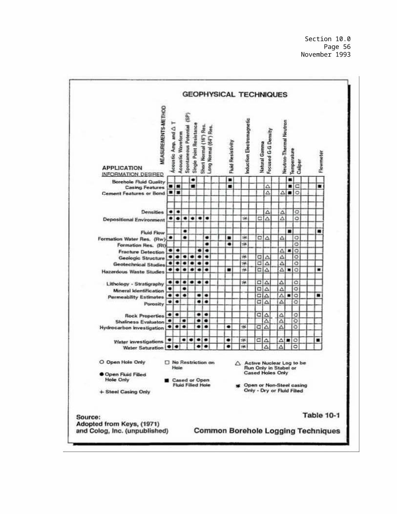
Section 10.0Page 57
November 1993
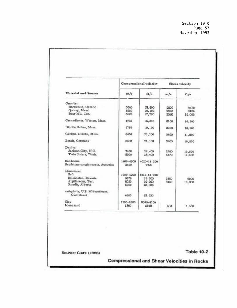
COMMONWEALTH OF MASSACHUSETTS
DEPARTMENT OF ENVIRONMENTAL PROTECTION
STANDARD REFERENCES FOR GEOPHYSICAL INVESTIGATIONS
SECTION 11.0 UNDERWATER METHODS
Section 11.0Page i
November 1993
SECTION 11.0UNDERWATER METHODS
TABLE OF CONTENTS
Section Title Page No.
11.1 OVERVIEW......................................... 1
11.2 INTRODUCTION..................................... 1
11.3 APPLICATIONS..................................... 1
11.3-1 Seismic Methods ................................. 111.3-2 Resistivity ..................................... 211.3-3 Self-Potential .................................. 211.3-4 Ground Penetrating Radar (GPR) .................. 211.3-5 Magnetics ....................................... 211.3-6 Microgravity .................................... 211.3-7 Borehole Geophysics ............................. 3
11.4 OTHER UNDERWATER METHODS......................... 3
11.4-1 Bathymetric Measurements......................... 3
11.4-1.1 Overview......................................... 311.4-1.2 Applications..................................... 411.4-1.3 Equipment........................................ 411.4-1.4 Field Procedures................................. 411.4-1.5 Interpretation................................... 4
11.4-1.5.1 Data Analysis.................................... 411.4-1.5.2 Presentation of Results.......................... 411.4-1.5.3 Interpretation of Results........................ 5
11.4-1.6 Advantages and Disadvantages..................... 5
11.4-2 Side Scan Sonar.................................. 5
11.4-2.1 Overview......................................... 511.4-2.2 Applications..................................... 611.4-2.3 Equipment........................................ 611.4-2.4 Field Procedures................................. 6
Section 11.0Page ii
November 1993
SECTION 11.0UNDERWATER METHODS
TABLE OF CONTENTS (continued)
Section Title Page No.
11.4-2.5 Interpretation.................................... 7
11.4-2.5.1 Data Analysis..................................... 711.4-2.5.2 Presentation of Results........................... 711.4-2.5.3 Interpretation of Results......................... 711.4-2.6 Advantages and Disadvantages...................... 7
11-5 GLOSSARY.......................................... 7
LIST OF FIGURES
Figures Title Page No.
11-1 Schematic for Continuous Seismic Refraction Profiling.......................................11
11-2 Seismic Reflection Method.......................12
(a) Geometry of Seismic Wave Ray Path .........12(b) Instrumentation............................12
11-3 Bathymetric Profile of a Reservoir Bottom ShowingLocation of a Sinkhole..........................13
11-4 Side-Scan Sonar Record .........................14
11-5 Side-Scan Sonar System..........................15
Section 11.0Page 1
November 1993
11.0 UNDERWATER METHODS
11.1 OVERVIEW
The collection of geological information (i.e., type of overburden material, depth to bedrock) from areas beneath rivers, ponds, tidal and inner harbor areas, where direct examination is logistically difficult, is often necessary. The location of objects (i.e., waste drums) present beneath water covered areas is also occasionally required. In these situations the use of geophysical techniques is often the most cost effective approach to data collection. Underwater/subaqueous geophysical surveys described below utilize most of the geophysical methodologies previously discussed in Sections 3.0 through 10.0 of these Standard References. In addition, presented below are two geophysical methods which are specific to only water-covered areas.
11.2 INTRODUCTION
For underwater geophysical work, land geophysical methods must generally be modified. Included below, in Section 11.3, are some of the modifications needed in order to use those land methods for underwater/subaqueous work. In addition, two methods specific to underwater application are considered in a detailed manner. It is noteworthy that some of the methods are towed systems (floating or slightly submerged), whereas, others will be individual station-type measurements made on the bottom.
11.3 APPLICATIONS
All the geophysical methods described below (with the exception of Bathymetry and Side Scan Sonar which are described in detail) have been described in detail in previous sections of Chapter 8. The following is therefore only an overview of the application of a geophysical technique to a marine setting. For a detailed description of a particular method, please refer to the sections referenced in the text.
11.3-1 Seismic Methods
Seismic refraction and reflection are both suitable for water-covered areas. For refraction surveys, the only modification is in the energy source, where explosives are replaced by a non-explosive source such as an air gun, which allows instantaneous release of high pressure air from a chamber. This is safer for personnel and prevents fish kills at the source. A schematic of the subaqueous seismic refraction method is shown on Figure 11-1. Refer also to Section 3.0 for further explanation of seismic methods.
Reflection profiling is much more prevalent for subaqueous environments than for land applications. High resolution units utilizing non-explosive energy sources (including: electromechanical "boomers", spark discharge "sparkers", and piezo-electric crystal "pingers") allow generation of high frequency energy that penetrates sub-bottom materials and allows continuous profiling of soil and bedrock layers. Data are re-
Section 11.0Page 2
November 1993
corded continuously utilizing a towed source and receiver array coupled with a recording unit on the survey vessel with direct, graphic recording and a provision for taping and subsequent playbacks. The subaqueous reflection method is illustrated on Figure 11-2.
11.3-2 Resistivity
The logistics of performing resistivity measurements in subaqueous environments are the only differences from land-type applications. Surveys can be performed with an array of electrodes, with variable or constant spacings, towed in a floating configuration or dragged across the ocean floor or lake bed of an area of interest. Data can be recorded on the same read-out unit utilized for land work or with a continuous recorder similar to the ones used for well logging operations (refer also to Section 10.0, Borehole Geophysics, and to Section 4.0, Resistivity).
11.3-3 Self-Potential
This technique has been widely utilized for identifying groundwater or leachate leakage/seepage into water-covered areas such as reservoirs and lakes or from impoundments and dams. In this instance, the reference electrode is placed in the water and the measurement electrode is placed at various locations along the shore.
Leachate moving from a landfill into an adjacent stream or pond could also be detected (refer also to Section 5.0). For this application the reference electrode is placed in the stream bank or shoreline and the measurement electrode is placed in the water and moved along the shoreline.
11.3-4 Ground Penetrating Radar (GPR)
Recent developments with GPR indicate its suitability in non-saline water-covered settings for high resolution evaluation of lithologies and for object detection. Subaqueous operations are similar to land-based work except that the antenna is towed in a floating configuration behind the boat carrying the recording equipment. For a further explanation of GPR, please refer to Section 7.0.
11.3-5 Magnetics
Magnetic surveys in water-covered areas are done by towing the sensor and utilizing a continuous chart recorder for the output signals. Magnetic surveys in subaqueous environments have a distinct advantage over land surveys in that they can be performed rapidly and continuously. They are especially useful for detecting dumped ferrous objects, such as barrels or other steel/iron debris. For further explanation of magnetic surveys, please refer to Section 8.0.
11.3-6 Microgravity
Microgravity, and gravimetric measurements in general, are difficult to
Section 11.0Page 3
November 1993
perform in subaqueous environments. The instrument must be positioned and leveled on a firm bottom surface at surveyed locations, unmoved by winds and waves. It is doubtful that any gravitational type of survey program will find widespread application for subaqueous involvements. For a description of microgravity applications on land, please refer to Section 9.0.
11.3-7 Borehole Geophysics
A number of borehole geophysical techniques previously covered under Section 10.0 can also be applied to subaqueous surveys by towing borehole geophysics equipment behind a boat in a floating configuration or by dragging them along the bottom of water-covered areas. Of particular significance are the electrical methods (resistivity, SP, electromagnetic/induction), the temperature log, and underwater television camera observations. The logistics of underwater applications are more involved than with typical borehole applications. Accurate positioning/locationing of equipment is an added requirement for successful underwater application.
11.4 OTHER UNDERWATER METHODS
Two methods appropriate for underwater applications, which are not directly related to the land-based geophysical techniques discussed above are:
o Bathymetry
o Side Scan Sonar
11.4-1 Bathymetric Measurements
11.4-1.1 Overview
Bathymetric measurements are made to determine the depths of water (or conversely ocean floor and lake bed elevations) in water-covered areas. The water surface becomes the plane of reference and accurate water depths are converted to bottom elevations. In tidal areas, where the water surface level exhibits significant fluctuations, a tidal gauge must be used to correct this plane of reference. Figure 11-3 is a copy of a bathymetric recording.
Typically, a fathometer is used to perform a Bathymetric Survey. The fathometer is, essentially, a precision depth sounder which measures and records the water depth from the surface to an object below. It records the depth at a point directly below the transducer (an acoustic energy transmitter/receiver), recording the points continuously on a strip chart as the boat advances. The water depth measurements are easy to perform; for example, the recording fathometers that many sport fishermen operate on their boats are adequate and reliable for water depth determinations in any pond or stream.
These surveys will often require accurate identification of geographical locations by either electronic navigation equipment or land survey
Section 11.0Page 4
November 1993
techniques.
11.4-1.2 Applications
The principal application for this technique is to determine water bottom elevations relative to the water surface plane of reference. When such measurements are performed monthly or annually changes due to sedimentation and/or dumping practices can be readily identified and assessed as to their lateral and vertical extent. In areas of dredging or excavation, such as for pipe lines and dredged channels, this measurement technique provides a rapid means of assessing changes in bottom elevations.
11.4-1.3 Equipment
A typical system for such measurements consist of a single transducer (a combined source and receiver, usually constructed from a piezoelectric element) and a chart recorder with a depth scale and provision for "mark" points at designated intervals as a surveying/locationing control person may indicate. The type of survey vessel used for bathymetric studies will range from small, portable boats (for ponds and rivers) to larger, sea-going vessels (for the deeper waters of harbors and near-shore ocean areas).
11.4-1.4 Field Procedures
The collection of data along a series of parallel lines or across a survey grid provides the best coverage for any water-covered area. The spacing of such line coverage will depend on the size and shape of the bottom conditions and bottom irregularities that may be anticipated, as well as survey requirements. Lines may be as close as 10 foot intervals in special cases, with 50- to 100-foot spacings used for deeper water areas of interest. For sites where elongated features such as dredged channels are of interest, the lines of measurement should be positioned perpendicular, if possible, to the elongated features.
11.4-1.5 Interpretation
11.4-1.5.1 Data Analysis
The chart recordings (see Figure 11-3) are scaled, transferring water depth values for each high point and each low point as well as for the points of inflection of bottom slopes observed on the recordings. A continuous profile and/or a tabulation of water depths is thereby determined for an area of interest, and surrounding locales if desired.
Also, these data can either be plotted on a plan map and contoured by hand, or a computer program can be used for the contouring of both depth and location coordinate data.
11.4-1.5.2 Presentation of Results
Results of bathymetric measurements are presented in the above noted
Section 11.0Page 5
November 1993
profile and contoured form, with spot point designations for localized highs or lows. The presentations should also include notations concerning map/location positions on the profiles, and geographic grid coordinates on the plan map types of data presentations. It may also be useful to designate other information, such as where bottom samples and/or drill holes were positioned.
11.4-1.5.3 Interpretation of Results
Interpretation of bathymetric recordings is generally straightforward. The data is either taken as a one time set of water depth/bottom elevation measurements or is compared to earlier and later results. The variations may be attributed to natural causes such as sedimentation or to manmade causes such as excavation or dumped objects.
11.4-1.6 Advantages and Disadvantages
Bathymetric measurements are a rapid and cost-effective means of determining bottom elevations and changes.
A disadvantage of the method is that data are obtained only in vertical profile along the line of traverse. Significant bottom irregularities that occur adjacent to a traverse are overlooked. This disadvantage can be overcome either by maintaining a much closer spacing of lines or by utilizing "Side Scan Sonar" (see Section 11.3-8.2 below).
A second disadvantage to this technique is that it does not determine type or thickness of material that comprises the lake bed or ocean bottom. To collect these data, another geophysics technique (e.g., seismic reflection) or direct measurement (e.g., push rod, ponar sampling) is necessary.
11.4-2 Side Scan Sonar
11.4-2.1 Overview
The side scan sonar method provides a rapid and reliable means of searching the bottom of a water-covered area for objects, determining the distribution of soil types (fine versus coarse) as they occur along the bottom, and evaluating bottom topography. This method is useful for the fullest evaluation of bottom topography and for locating sunken objects. Side scan sonar recordings can also be used to create water depth profiles, if the measurement equipment, which is towed behind a boat, is maintained at a relatively constant depth below the surface of the water.
Section 11.0Page 6
November 1993
A set of two separate transducers mounted in a compact tow unit (known as a "fish") emit high power, short duration acoustic pulses (in a narrow, fan-shaped beam) that travel downward in a plane perpendicular to the tow "fish" travel path. As the boat moves forward, successive energy transmissions generate continuous ocean bottom or lake bed coverage data (with lateral extent governed by the maximum system range). Acoustic energy reflected from the bottom is received by the transducers in the "fish" and transmitted as electrical energy to the recorder; data are then amplified, processed, and converted to hard copy.
The scanning procedure allows a large spacing interval for the lines, providing considerable coverage in a small amount of time. It is suitable for ponds and rivers as well as for near-shore and deeper ocean areas.
11.4-2.2 Applications
This method is primarily a searching technique; it provides data that are analogous to low-angle photography on land, oblique (above and to the side of) to the objects of interest. The "fish" can search the sea floor on either side of the survey vessel from as close as 30 meters up to approximately five kilometers. Objects that protrude from the ocean floor, as well as ocean floor depressions are readily distinguishable. Dumped debris, such as barrels or trash, are discernible in waters that are too murky for direct observation from the surface or by diving. Although the technique has been most often used in deep water and offshore operations, recent experience in water depths of less than ten feet has confirmed its usefulness for environmental purposes involving shallow ponds, lakes, bays and estuaries.
11.4-2.3 Equipment
A towed transducer, usually referred to as a sonar "fish," is connected to a graphic, two-channel recorder that displays the scanning sonar signals both from the left and right directions of the course of traverse, as illustrated on Figure 11-4. Tape recording for later pro-cessing can also be utilized, although it is doubtful that many environmental projects will have need of such sophistication. The size of the boat needed for towing is governed by the water conditions and size of the survey area.
11.4-2.4 Field Procedures
Lines of traverse are spaced at approximately 100- to 200-foot intervals, which allows overlapping coverage from a left scan and a right scan. For most site settings, lines of operation are oriented in a single direction with allowance for cross check lines for specific features of interest, such as a debris pile or unknown object of environmental concern. As with bathymetric surveys, the side scan sonar surveys require accurate geographical orientation. This can be performed with either electronic navigation positioning equipment or land survey techniques.
Section 11.0Page 7
November 1993
11.4-2.5 Interpretation
11.4-2.5.1 Data Analysis
Inspection of field recordings by an experienced observer is usually adequate to identify subaqueous features of interest.
11.4-2.5.2 Presentation of Results
The positions of subaqueous features are transferred to site plan maps for a given area including geographical coordinates. Notations of the sizes and shapes of objects and trends of bottom features, such as scour channels or sand waves, are added. A track line map for the area of survey coverage is augmented with designations for detected objects of interest.
11.4-2.5.3 Interpretation of Results
In addition to using the data to search for objects and define bottom topographic trends, information about bottom geologic conditions, such as the presence or absence of sand waves, boulder trains, and channels, is readily obtained.
11.4-2.6 Advantages and Disadvantages
The advantage of this survey method is that it is rapid, covers a large amount of area in a relatively small time period and may provide a unique type of data.
A disadvantage of the method is that the specific identity of an object cannot be determined. Dumped containers may have the appearance of blocks of rock or boulders and may require direct observation for verification.
11.5 GLOSSARY
Bathymetry - Determination, with a fathometer, of water depths and corresponding bottom elevations, referenced to a known plane such as the water surface.
Fathometer - A device which utilizes high frequency sound waves generated by a small energy source, a transducer. The sound waves are beamed toward and reflect from the water bottom. The time that the waves take to travel down and back are converted to distance/depth and displayed on a chart recorder or by a flashing light display.
"Fish" - A towed transducer/receiver array used in Sonar surveys.
Sonar - Use of acoustic signals as propagating waves through the water zone of water-covered areas for the purpose of object location.
Side scan - A sonar method with directional control of the propagated high frequency sound signals.

Section 11.0Page 8
November 1993
Transducer - A device which converts electrical energy into acoustic energy and vice versa.
Underwater/subaqueous - These terms are generally synonymous for both shallow and deep water investigations; they refer to sites which may be partially or totally covered by water.

Section 11.0Page 9
November 1993
REFERENCES
Edgerton, H.E., 1986, Sonar images: Old Tappan, NJ, Prentice-Hall, 224 p. Ingham, A.E., 1974, Hydrography for the surveyor and engineer: New York,
NY, John Wiley, 139 p.
Trabant, P.K., 1984, Applied high-resolution geophysical methods: Boston, MA, International Human Resources Development Corporation, 265 p.

Section 11.0Page 10
November 1993
SECTION 11.0UNDERWATER METHODS
LIST OF FIGURES
Figures Title Page No.
11-1 Schematic for Continuous Seismic Refraction Profiling.......................................11
11-2 Seismic Reflection Method.......................12
(a) Geometry of Seismic Wave Ray Path..........12(b) Instrumentation............................12
11-3 Bathymetric Profile of a Reservoir Bottom ShowingLocation of a Sinkhole..........................13
11-4 Side-scan Sonar Record..........................14
11-5 Side-scan Sonar System..........................15
Section 11.0Page 11
November 1993
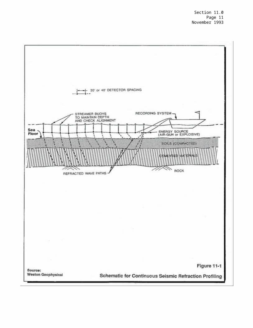
Section 11.0Page 12
November 1993
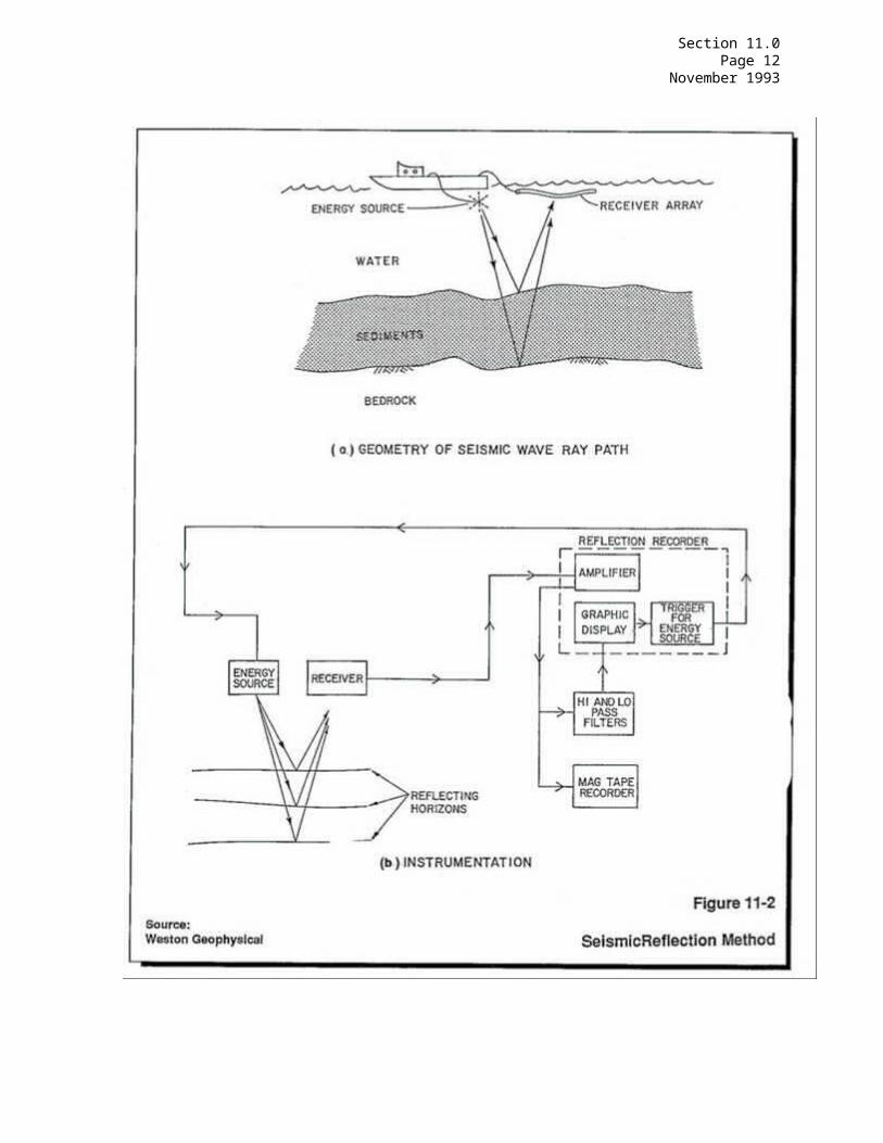
Section 11.0Page 13
November 1993
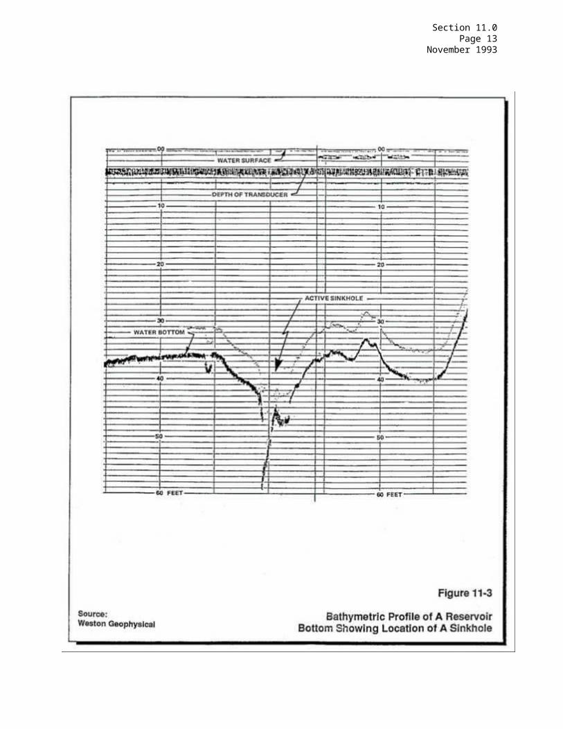
Section 11.0Page 14
November 1993
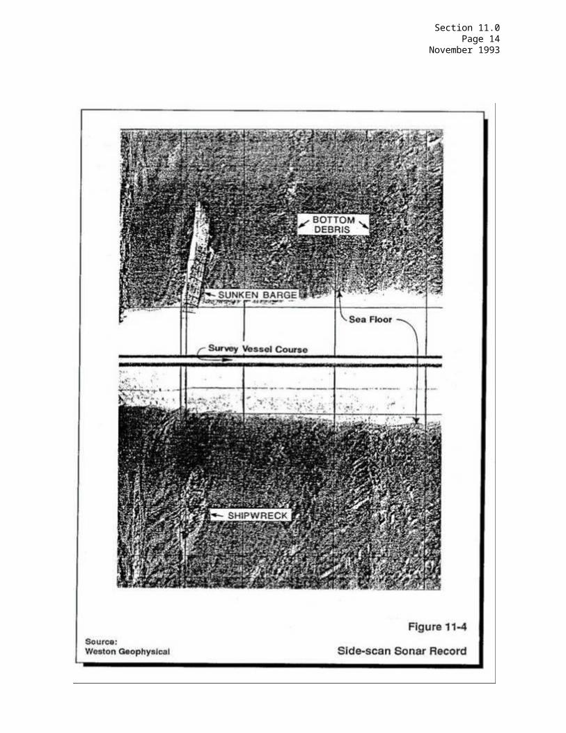
Section 11.0Page 15
November 1993