Lesson 7.1

In Chapter 1, you studied arithmetic sequences, which have a common difference between consecutive terms. This common difference is the slope of a line through the graph of the points. So, if you choose x-values along the line that form an arithmetic sequence, the corresponding y-values will also form an arithmetic sequence.

You have also studied several kinds of nonlinear sequences and functions, which do not have a common difference or a constant slope.

In this lesson you will discover that even nonlinear sequences sometimes have a special pattern in their differences.

These patterns are often described by polynomials.

When a polynomial is set equal to a second variable, such as y, it defines a polynomial function.

The degree of a polynomial or polynomial function is the power of the term that has the greatest exponent. ◦Linear Functions: y=3-2x

largest power of x is 1◦Cubic Function: y=2x3+1x2-2x+3

largest power of x is 3 If the degrees of the terms of a polynomial

decrease from left to right, the polynomial is in general form.

A polynomial that has only one term is called a monomial.

A polynomial with two terms is a binomial. A polynomial with three terms is a

trinomial. Polynomials with more than three terms are

usually just called “polynomials.”

In modeling linear functions, you have already discovered that for x-values that are evenly spaced, the differences between the corresponding y-values must be the same.

With 2nd- and 3rd-degree polynomial functions, the differences between the corresponding y-values are not the same. However, finding the differences between those differences produces an interesting pattern.

For the 2nd-degree polynomial function, the D2 values are constant, and for the 3rd-degree polynomial function, the D3 values are constant. What do you think will happen with a 4th- or 5th-degree polynomial function?

Analyzing differences to find a polynomial’s degree is called the finite differences method. You can use this method to help find the equations of polynomial functions modeling certain sets of data.

Find a polynomial function that models the relationship between the number of sides and the number of diagonals of a convex polygon. Use the function to find the number of diagonals of a dodecagon (a 12-sided polygon).

You need to create a table of values with evenly spaced x-values. Sketch polygons with increasing numbers of sides. Then draw all of their diagonals.

• Let x be the number of sides and y be the number of diagonals.

• You may notice a pattern in the number of diagonals that will help you extend your table beyond the sketches you make.

• Calculate the finite differences to determine the degree of the polynomial function.

You can stop finding differences when the values of a set of differences are constant. Because the values of D2 are constant, you can model the data with a 2nd-degree polynomial function like y =ax2 + bx + c.

To find the values of a, b, and c, you need a system of three equations.

Choose three of the points from your table, say (4, 2), (6, 9), and (8, 20), and substitute the coordinates into y =ax2 + bx + c to create a system of three equations in three variables. Can you see how these three equations were created?

16 4 2

36 6 9

64 8 20

a b c

a b c

a b c

16 4 2

36 6 9

64 8 20

a b c

a b c

a b c

16 4 1

36 6 1

64 8 1

a

b

c

2

9

20

=

16 4 1

36 6 1

64 8 1

a

b

c

2

9

20

=

116 4 1

36 6 1

64 8 1

116 4 1

36 6 1

64 8 1

a

b

c

0.5

1.5

0

=

Solve the system to find a=0.5, b=-1.5, and c=0.

Use these values to write the function y=0.5x2-1.5x.

This equation gives the number of diagonals of any polygon as a function of the number of sides.

Now substitute 12 for x to find that a dodecagon has 54 diagonals. 2

2

0.5 1.5

0.5(12) 1.5(12)

54

y x x

y

y

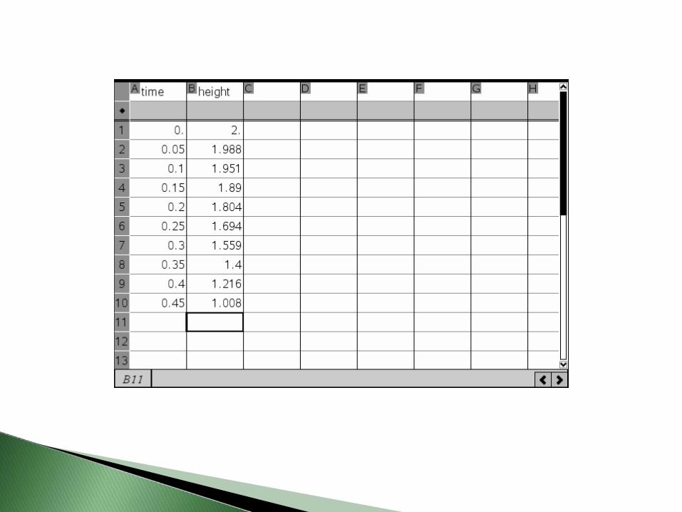
What function models the height of an object falling due to the force of gravity? Use a motion sensor to collect data, and analyze the data to find a function.

1. Set the sensor to collect distance data approximately every 0.05 s for 2 to 5 s.

2. Place the sensor on the floor. Hold a small pillow at a height of about 2 m, directly above the sensor.

3. Start the sensor and drop the pillow.

Let x represent time in seconds, and let y represent height in meters. Select about 10 points from the free-fall portion of your data, with x-values forming an arithmetic sequence. Record this information in a table. Round all heights to the nearest 0.001.

Create scatter plots of the original data (time, height), then a scatter plot of (time, first difference), and finally a scatter plot of (time, second difference).

Write a description of each graph from the previous step and what these graphs tell you about the data.

The graph of (time, height) appears parabolic and suggests that the correct model may be a quadratic (2nd-degree) polynomial function. The graph of (time, first difference) shows that the first differences are not constant; because they decrease in a linear fashion, the second differences are likely to be constant. The graph of (time, second difference) shows that the second differences are nearly constant, so the correct model should be a 2nd-degree polynomial function.

Based on your results from using finite differences, what is the degree of the polynomial function that models free fall? Write the general form of this polynomial function.

2nd degree: y=ax2 +bx+c

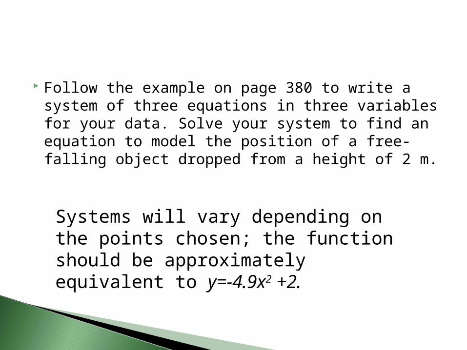
Follow the example on page 380 to write a system of three equations in three variables for your data. Solve your system to find an equation to model the position of a free- falling object dropped from a height of 2 m.

Systems will vary depending on the points chosen; the function should be approximately equivalent to y=-4.9x2 +2.

Use the finite differences method to find the degree of the polynomial function that models your data. Stop when the differences are nearly constant.

There are two ways you can find the finite differences: ◦ From the table of values◦ From the homescreen

• First

• First name Column C: diff1 and Column D: diff2

• Then in the gray row enter the command Δlist(height) in column C and Δlist(diff1) in column D

• What do you notice about the second differences?

Create scatter plots of the original data (time, height), then a scatter plot of (time, first difference), and finally a scatter plot of (time, second difference).

Write a description of each graph from the previous step and what these graphs tell you about the data.

The graph of (time, height) appears parabolic and suggests that the correct model may be a quadratic (2nd-degree) polynomial function. The graph of (time, first difference) shows that the first differences are not constant; because they decrease in a linear fashion, the second differences are likely to be constant. The graph of (time, second difference) shows that the second differences are nearly constant, so the correct model should be a 2nd-degree polynomial function.

Based on your results from using finite differences, what is the degree of the polynomial function that models free fall? Write the general form of this polynomial function.

2nd degree: y = ax2 + bx + c

Follow the example on page 380 to write a system of three equations in three variables for your data. Solve your system to find an equation to model the position of a free- falling object dropped from a height of 2 m.

Systems will vary depending on the points chosen; the function should be approximately equivalent to y=-4.9x2 +2.

Let’s select (0,2), (0.2, 1.804) and (0.4, 1.216) as the three points.

Replacing these in the equation y = ax2 + bx + c we get ◦ 2=0a+0b+c◦ 1.804=0.04a+0.2b+c◦ 1.216=0.16a+0.4b+c

Y=-4.9x2+2