Lesson 29: Analysis of plane frame by stiffness methodnptel.ac.in/courses/Webcourse-contents/IIT Kharagpur...Instructional Objectives After reading this chapter the student will be

Module 4

Analysis of Statically Indeterminate

Structures by the Direct Stiffness Method

Version 2 CE IIT, Kharagpur

Lesson 30

The Direct Stiffness Method: Plane Frames


Instructional Objectives After reading this chapter the student will be able to 1. Derive plane frame member stiffness matrix in local co-ordinate system. 2. Transform plane frame member stiffness matrix from local to global co-

ordinate system. 3. Assemble member stiffness matrices to obtain the global stiffness matrix of

the plane frame. 4. Write the global load-displacement relation for the plane frame. 5. Impose boundary conditions on the load-displacement relation. 6. Analyse plane frames by the direct stiffness matrix method. 30.1 Introduction In the case of plane frame, all the members lie in the same plane and are interconnected by rigid joints. The internal stress resultants at a cross-section of a plane frame member consist of bending moment, shear force and an axial force. The significant deformations in the plane frame are only flexural and axial. In this lesson, the analysis of plane frame by direct stiffness matrix method is discussed. Initially, the stiffness matrix of the plane frame member is derived in its local co-ordinate axes and then it is transformed to global co-ordinate system. In the case of plane frames, members are oriented in different directions and hence before forming the global stiffness matrix it is necessary to refer all the member stiffness matrices to the same set of axes. This is achieved by transformation of forces and displacements to global co-ordinate system. 30.2 Member Stiffness Matrix Consider a member of a plane frame as shown in Fig. 30.1a in the member co-ordinate system ' . The global orthogonal set of axes '' zyx xyz is also shown in the figure. The frame lies in the xy plane. The member is assumed to have uniform flexural rigidity EI and uniform axial rigidity EA for sake of simplicity. The axial deformation of member will be considered in the analysis. The possible displacements at each node of the member are: translation in - and - direction and rotation about - axis.

'x 'y'z


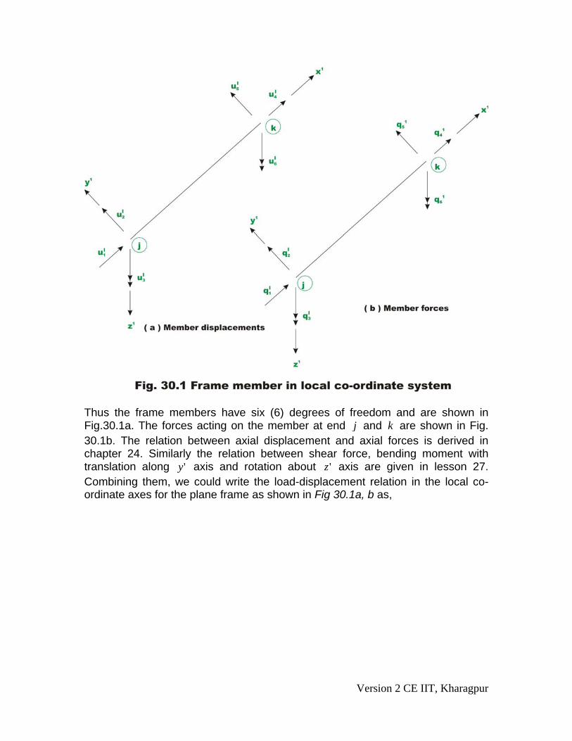
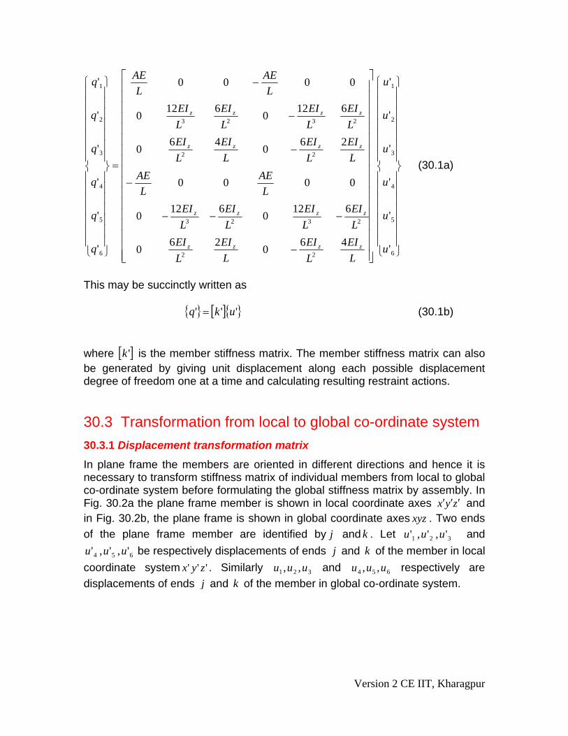
Thus the frame members have six (6) degrees of freedom and are shown in Fig.30.1a. The forces acting on the member at end j and are shown in Fig. 30.1b. The relation between axial displacement and axial forces is derived in chapter 24. Similarly the relation between shear force, bending moment with translation along axis and rotation about axis are given in lesson 27. Combining them, we could write the load-displacement relation in the local co-ordinate axes for the plane frame as shown in Fig 30.1a, b as,

k

'y 'z


⎪⎪⎪⎪⎪⎪⎪

⎭

⎪⎪⎪⎪⎪⎪⎪

⎬

⎫

⎪⎪⎪⎪⎪⎪⎪

⎩

⎪⎪⎪⎪⎪⎪⎪

⎨

⎧

⎥⎥⎥⎥⎥⎥⎥⎥⎥⎥⎥⎥⎥⎥⎥⎥⎥

⎦

⎤

⎢⎢⎢⎢⎢⎢⎢⎢⎢⎢⎢⎢⎢⎢⎢⎢⎢

⎣

⎡

−

−−−

−

−

−

−

=

⎪⎪⎪⎪⎪⎪⎪

⎭

⎪⎪⎪⎪⎪⎪⎪

⎬

⎫

⎪⎪⎪⎪⎪⎪⎪

⎩

⎪⎪⎪⎪⎪⎪⎪

⎨

⎧

6

5

4

3

2

1

22

2323

22

2323

6

5

4

3

2

1

'

'

'

'

'

'

460

260

6120

6120

0000

260

460

6120

6120

0000

'

'

'

'

'

'

u

u

u

u

u

u

LEI

LEI

LEI

LEI

LEI

LEI

LEI

LEI

LAE

LAE

LEI

LEI

LEI

LEI

LEI

LEI

LEI

LEI

LAE

LAE

q

q

q

q

q

q

zzzz

zzzz

zzzz

zzzz

(30.1a)

This may be succinctly written as

{ } [ ]{ }''' ukq = (30.1b) where is the member stiffness matrix. The member stiffness matrix can also be generated by giving unit displacement along each possible displacement degree of freedom one at a time and calculating resulting restraint actions.

[ ]'k

30.3 Transformation from local to global co-ordinate system 30.3.1 Displacement transformation matrix

In plane frame the members are oriented in different directions and hence it is necessary to transform stiffness matrix of individual members from local to global co-ordinate system before formulating the global stiffness matrix by assembly. In Fig. 30.2a the plane frame member is shown in local coordinate axes zyx ′′′ and in Fig. 30.2b, the plane frame is shown in global coordinate axes xyz . Two ends of the plane frame member are identified by j and . Let and

be respectively displacements of ends k 321 ',',' uuu

654 ',',' uuu j and of the member in local coordinate system ' . Similarly and respectively are displacements of ends

k'' zyx 321 ,, uuu 654 ,, uuuj and k of the member in global co-ordinate system.


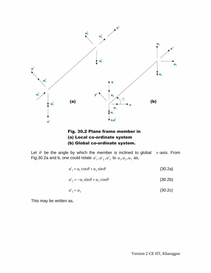
Let θ be the angle by which the member is inclined to global x -axis. From Fig.30.2a and b, one could relate to as, 321 ',',' uuu 321 ,, uuu

θθ sincos' 211 uuu += (30.2a)

θθ cossin' 212 uuu +−= (30.2b)

33' uu = (30.2c) This may be written as,


⎪⎪⎪⎪⎪

⎭

⎪⎪⎪⎪⎪

⎬

⎫

⎪⎪⎪⎪⎪

⎩

⎪⎪⎪⎪⎪

⎨

⎧

⎥⎥⎥⎥⎥⎥⎥⎥⎥⎥

⎦

⎤

⎢⎢⎢⎢⎢⎢⎢⎢⎢⎢

⎣

⎡

−

−

=

⎪⎪⎪⎪⎪

⎭

⎪⎪⎪⎪⎪

⎬

⎫

⎪⎪⎪⎪⎪

⎩

⎪⎪⎪⎪⎪

⎨

⎧

6

5

4

3

2

1

6

5

4

3

2

1

100000

0000

0000

000100

0000

0000

'

'

'

'

'

'

u

u

u

u

u

u

lm

ml

lm

ml

u

u

u

u

u

u

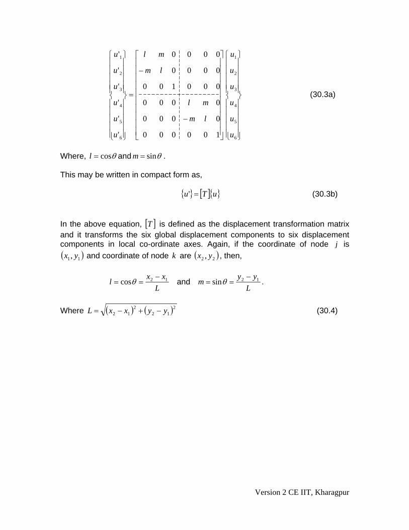
(30.3a)

Where, θcos=l and θsin=m . This may be written in compact form as,

{ } [ ]{ }uTu =' (30.3b) In the above equation, [ is defined as the displacement transformation matrix and it transforms the six global displacement components to six displacement components in local co-ordinate axes. Again, if the coordinate of node

]T

j is and coordinate of node are ( 11, yx ) k ( )22 , yx , then,

Lxxl 12cos −

== θ and L

yym 12sin −== θ .

Where ( ) ( )2

122

12 yyxxL −+−= (30.4)


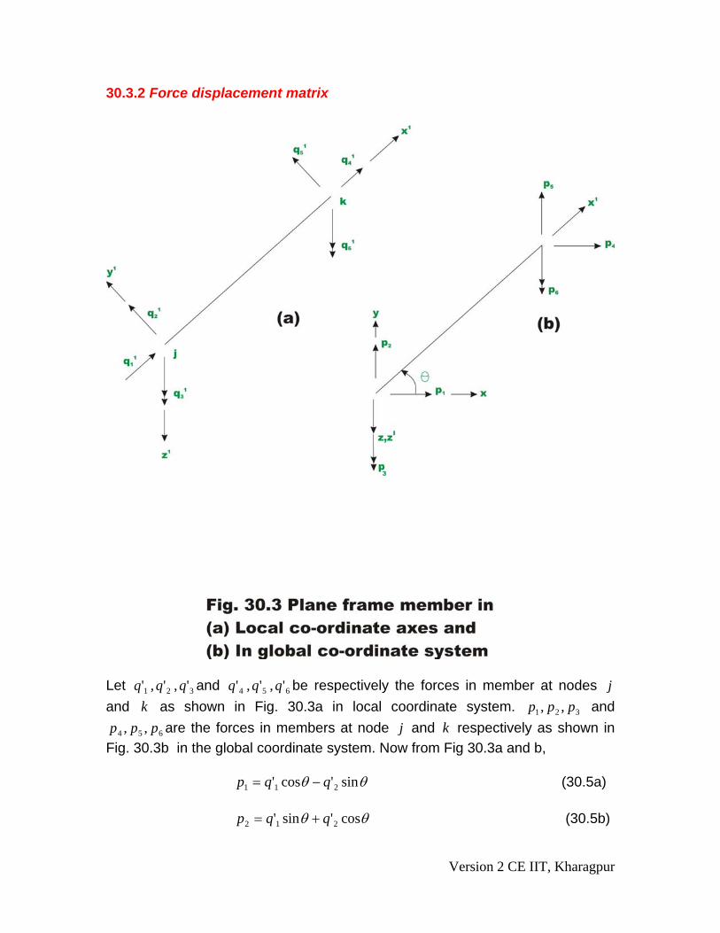
30.3.2 Force displacement matrix

Let and be respectively the forces in member at nodes 321 ',',' qqq 654 ',',' qqq j and as shown in Fig. 30.3a in local coordinate system. and

are the forces in members at node k 321 ,, ppp

654 ,, ppp j and respectively as shown in Fig. 30.3b in the global coordinate system. Now from Fig 30.3a and b,

k

θθ sin'cos' 211 qqp −= (30.5a)

θθ cos'sin' 212 qqp += (30.5b)


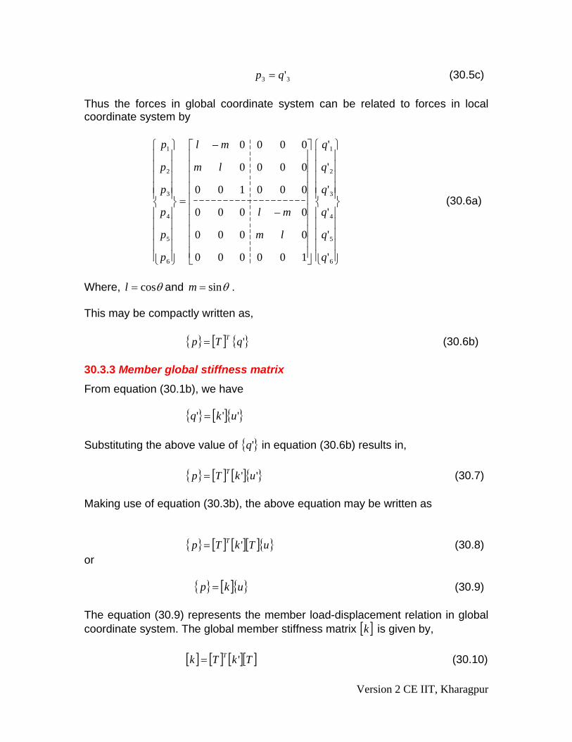
33 'qp = (30.5c) Thus the forces in global coordinate system can be related to forces in local coordinate system by

⎪⎪⎪⎪⎪

⎭

⎪⎪⎪⎪⎪

⎬

⎫

⎪⎪⎪⎪⎪

⎩

⎪⎪⎪⎪⎪

⎨

⎧

⎥⎥⎥⎥⎥⎥⎥⎥⎥⎥

⎦

⎤

⎢⎢⎢⎢⎢⎢⎢⎢⎢⎢

⎣

⎡

−

−

=

⎪⎪⎪⎪⎪

⎭

⎪⎪⎪⎪⎪

⎬

⎫

⎪⎪⎪⎪⎪

⎩

⎪⎪⎪⎪⎪

⎨

⎧

6

5

4

3

2

1

6

5

4

3

2

1

'

'

'

'

'

'

100000

0000

0000

000100

0000

0000

q

q

q

q

q

q

lm

ml

lm

ml

p

p

p

p

p

p

(30.6a)

Where, θcos=l and θsin=m . This may be compactly written as,

{ } [ ] { }'qTp T= (30.6b) 30.3.3 Member global stiffness matrix

From equation (30.1b), we have

{ } [ ]{ }''' ukq = Substituting the above value of { }'q in equation (30.6b) results in,

{ } [ ] [ ]{ }'' ukTp T= (30.7) Making use of equation (30.3b), the above equation may be written as

{ } [ ] [ ][ ]{ }uTkTp T '= (30.8) or

{ } [ ]{ }ukp = (30.9) The equation (30.9) represents the member load-displacement relation in global coordinate system. The global member stiffness matrix [ ]k is given by,

[ ] [ ] [ ][ ]TkTk T '= (30.10)


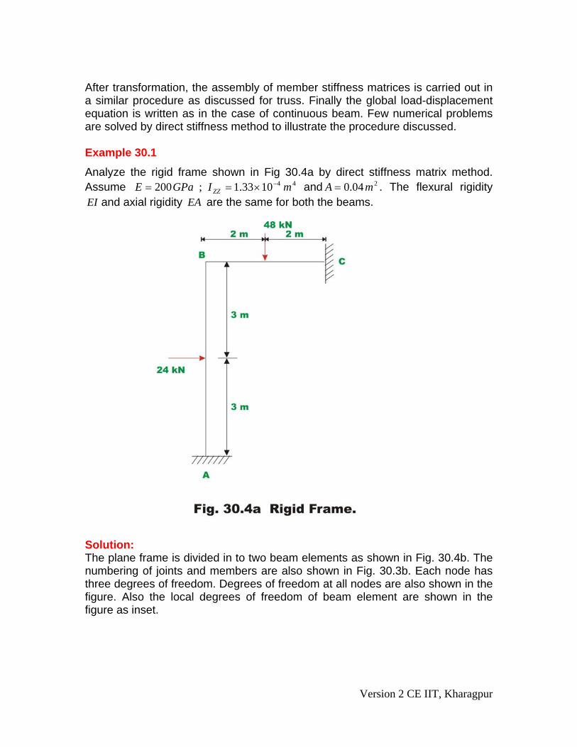
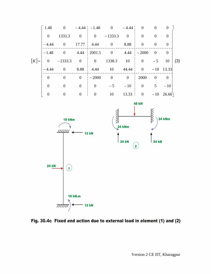
After transformation, the assembly of member stiffness matrices is carried out in a similar procedure as discussed for truss. Finally the global load-displacement equation is written as in the case of continuous beam. Few numerical problems are solved by direct stiffness method to illustrate the procedure discussed. Example 30.1 Analyze the rigid frame shown in Fig 30.4a by direct stiffness matrix method. Assume and . The flexural rigidity 441033.1;200 mIGPaE ZZ

−×== 204.0 mA =EI and axial rigidity EA are the same for both the beams.

Solution: The plane frame is divided in to two beam elements as shown in Fig. 30.4b. The numbering of joints and members are also shown in Fig. 30.3b. Each node has three degrees of freedom. Degrees of freedom at all nodes are also shown in the figure. Also the local degrees of freedom of beam element are shown in the figure as inset.


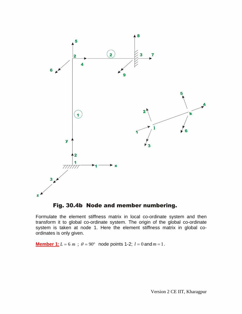
Formulate the element stiffness matrix in local co-ordinate system and then transform it to global co-ordinate system. The origin of the global co-ordinate system is taken at node 1. Here the element stiffness matrix in global co-ordinates is only given. Member 1: °== 90;6 θmL node points 1-2; 0=l and 1=m .


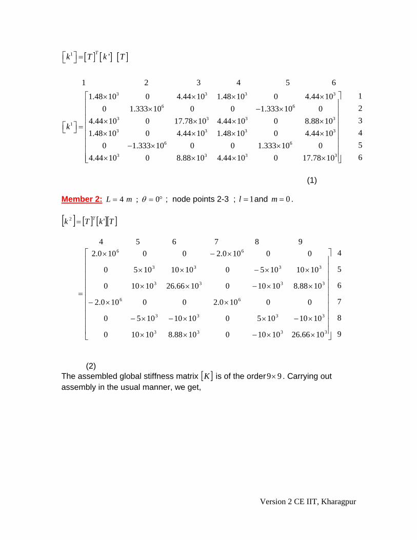
[ ] [ ] [ ]1 'Tk T k T⎡ ⎤ =⎣ ⎦

3 3 3 3

6 6

3 3 31

3 3 3 3

6 6

3 3 3

1 2 3 4 5 6

1.48 10 0 4.44 10 1.48 10 0 4.44 100 1.333 10 0 0 1.333 10 0

4.44 10 0 17.78 10 4.44 10 0 8.88 101.48 10 0 4.44 10 1.48 10 0 4.44 10

0 1.333 10 0 0 1.333 10 04.44 10 0 8.88 10 4.44 10 0 17.

k

× × × ×× − ×

× × × ×⎡ ⎤ =⎣ ⎦ × × × ×

− × ×× × × 3

12345678 10

⎡ ⎤⎢ ⎥⎢ ⎥⎢ ⎥⎢ ⎥⎢ ⎥⎢ ⎥⎢ ⎥

×⎢ ⎥⎣ ⎦

3

(1) Member 2: °== 0;4 θmL ; node points 2-3 ; 1=l and 0=m . [ ] [ ] [ ][ ]

9

8

7

6

5

4

1066.26101001088.810100

1010105010101050

00100.200100.2

1088.8101001066.2610100

1010105010101050

00100.200100.2987654

'

3333

3333

66

3333

3333

66

2

⎥⎥⎥⎥⎥⎥⎥⎥⎥⎥

⎦

⎤

⎢⎢⎢⎢⎢⎢⎢⎢⎢⎢

⎣

⎡

××−××

×−××−×−

××−

××−××

××−××

×−×

=

= TkTk T

(2) The assembled global stiffness matrix [ ]K is of the order 99× . Carrying out assembly in the usual manner, we get,


[ ]

⎥⎥⎥⎥⎥⎥⎥⎥⎥⎥⎥⎥⎥⎥⎥⎥

⎦

⎤

⎢⎢⎢⎢⎢⎢⎢⎢⎢⎢⎢⎢⎢⎢⎢⎢

⎣

⎡

−

−−−

−

−−

−−

−−

−

−

−−−

=

66.2610033.13100000

10501050000

002000002000000

33.1310044.441044.488.8044.4

1050103.1338003.13330

00200044.405.200144.4048.1

00088.8044.477.17044.4

00003.1333003.13330

00044.4048.144.4048.1

K (3)



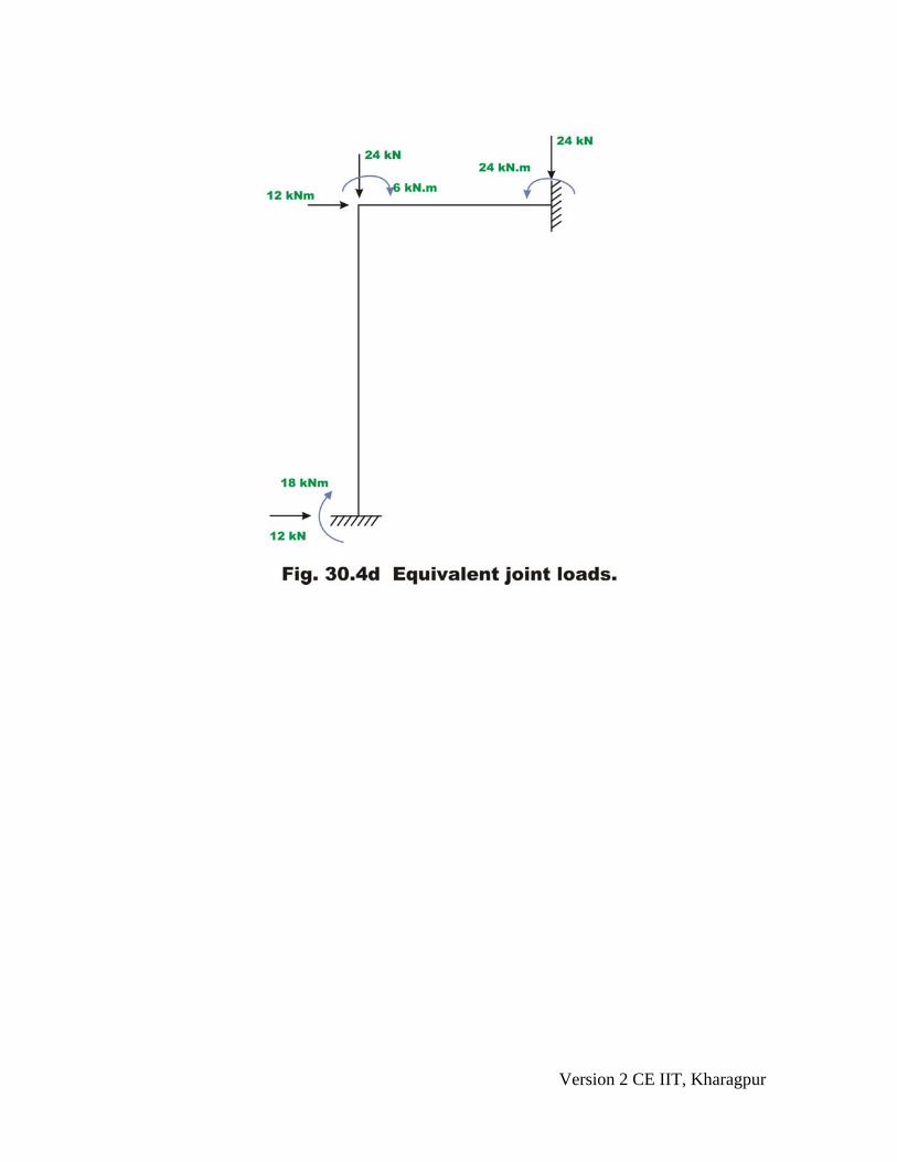
The load vector corresponding to unconstrained degrees of freedom is (vide 30.4d),

{ }⎪⎪⎭

⎪⎪⎬

⎫

⎪⎪⎩

⎪⎪⎨

⎧

−

−=

⎪⎪⎭

⎪⎪⎬

⎫

⎪⎪⎩

⎪⎪⎨

⎧

=

6

24

12

6

5

4

p

p

p

pk (4)

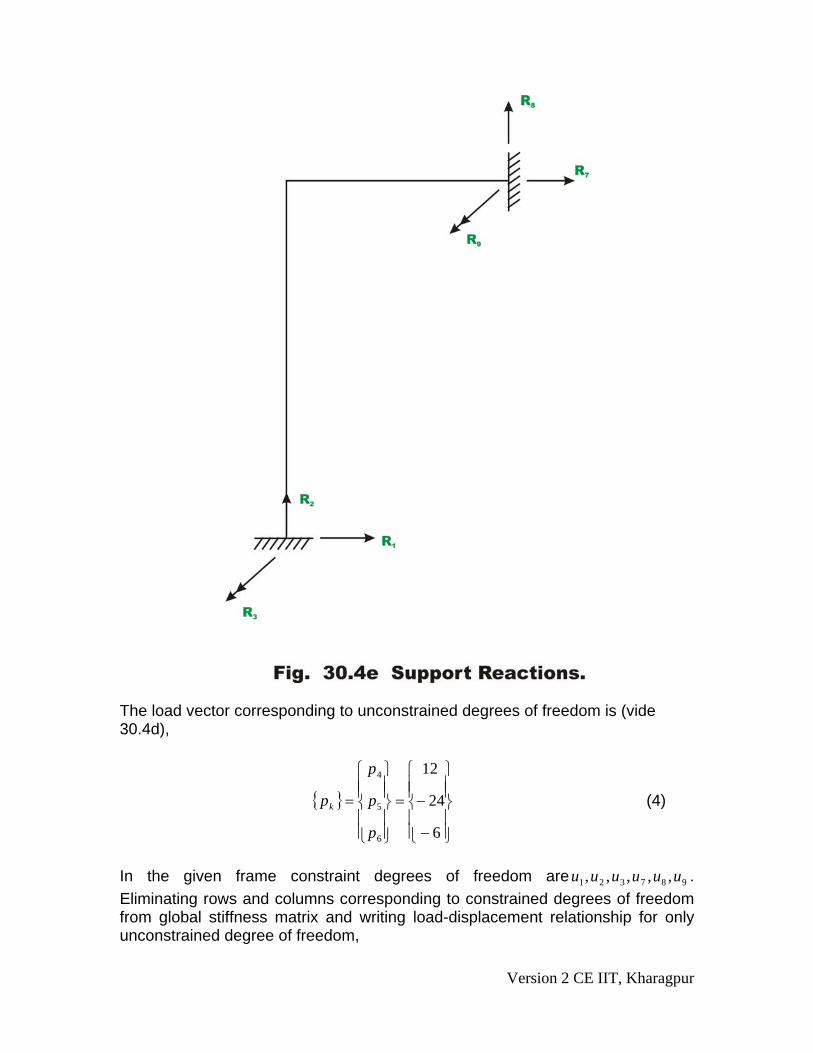
In the given frame constraint degrees of freedom are . Eliminating rows and columns corresponding to constrained degrees of freedom from global stiffness matrix and writing load-displacement relationship for only unconstrained degree of freedom,

987321 ,,,,, uuuuuu


⎪⎪⎭

⎪⎪⎬

⎫

⎪⎪⎩

⎪⎪⎨

⎧

⎥⎥⎥⎥

⎦

⎤

⎢⎢⎢⎢

⎣

⎡

=

⎪⎪⎭

⎪⎪⎬

⎫

⎪⎪⎩

⎪⎪⎨

⎧

−

−

6

5

4

3

44.441044.4

103.13380

44.405.2001

10

6

24

12

u

u

u

(5)

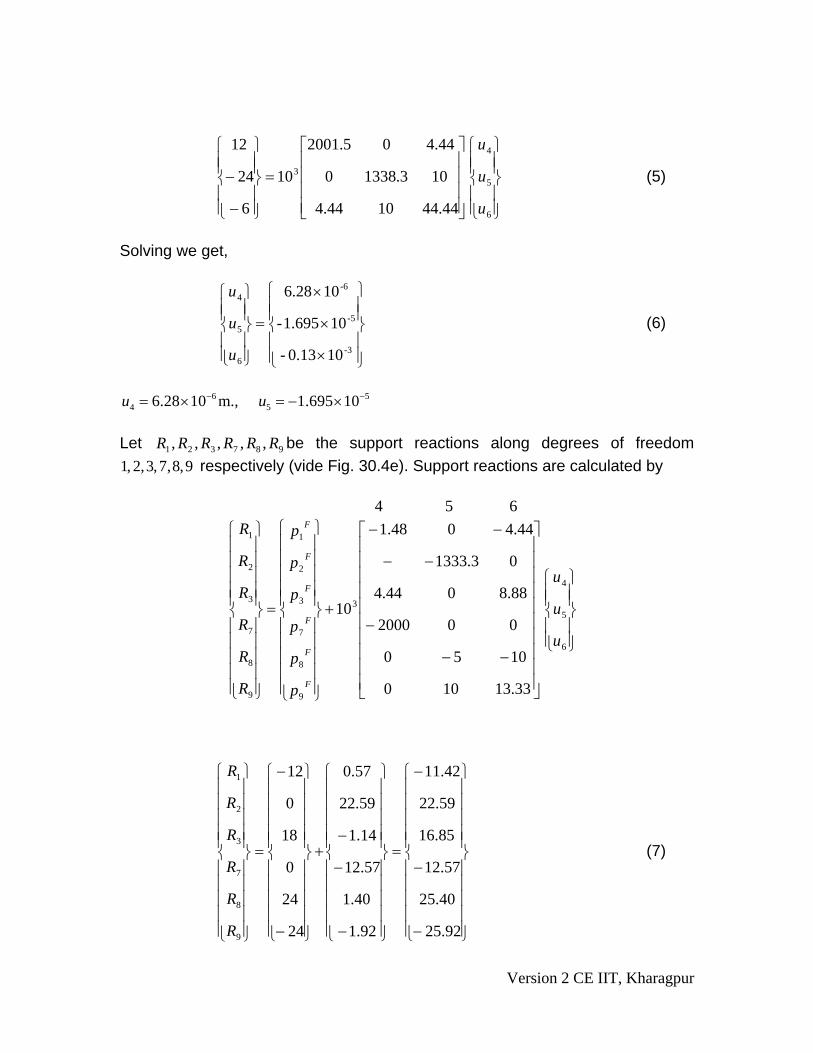
Solving we get,

⎪⎪⎭

⎪⎪⎬

⎫

⎪⎪⎩

⎪⎪⎨

⎧

×

×

×

=

⎪⎪⎭

⎪⎪⎬

⎫

⎪⎪⎩

⎪⎪⎨

⎧

3-

5-

-6

6

5

4

100.13-

101.695-

106.28

u

u

u

(6)

6 5

4 56.28 10 m., 1.695 10u u− −= × = − × Let be the support reactions along degrees of freedom

respectively (vide Fig. 30.4e). Support reactions are calculated by 987321 ,,,,, RRRRRR

9,8,7,3,2,1

⎪⎪⎭

⎪⎪⎬

⎫

⎪⎪⎩

⎪⎪⎨

⎧

⎥⎥⎥⎥⎥⎥⎥⎥⎥⎥

⎦

⎤

⎢⎢⎢⎢⎢⎢⎢⎢⎢⎢

⎣

⎡

−−

−

−−

−−

+

⎪⎪⎪⎪⎪

⎭

⎪⎪⎪⎪⎪

⎬

⎫

⎪⎪⎪⎪⎪

⎩

⎪⎪⎪⎪⎪

⎨

⎧

=

⎪⎪⎪⎪⎪

⎭

⎪⎪⎪⎪⎪

⎬

⎫

⎪⎪⎪⎪⎪

⎩

⎪⎪⎪⎪⎪

⎨

⎧

6

5

4

3

9

8

7

3

2

1

9

8

7

3

2

1

33.13100

1050

002000

88.8044.4

03.1333

44.4048.1

10

654

u

u

u

p

p

p

p

p

p

R

R

R

R

R

R

F

F

F

F

F

F

⎪⎪⎪⎪⎪

⎭

⎪⎪⎪⎪⎪

⎬

⎫

⎪⎪⎪⎪⎪

⎩

⎪⎪⎪⎪⎪

⎨

⎧

−

−

−

=

⎪⎪⎪⎪⎪

⎭

⎪⎪⎪⎪⎪

⎬

⎫

⎪⎪⎪⎪⎪

⎩

⎪⎪⎪⎪⎪

⎨

⎧

−

−

−+

⎪⎪⎪⎪⎪

⎭

⎪⎪⎪⎪⎪

⎬

⎫

⎪⎪⎪⎪⎪

⎩

⎪⎪⎪⎪⎪

⎨

⎧

−

−

=

⎪⎪⎪⎪⎪

⎭

⎪⎪⎪⎪⎪

⎬

⎫

⎪⎪⎪⎪⎪

⎩

⎪⎪⎪⎪⎪

⎨

⎧

92.25

40.25

57.12

85.16

59.22

42.11

92.1

40.1

57.12

14.1

59.22

57.0

24

24

0

18

0

12

9

8

7

3

2

1

R

R

R

R

R

R

(7)


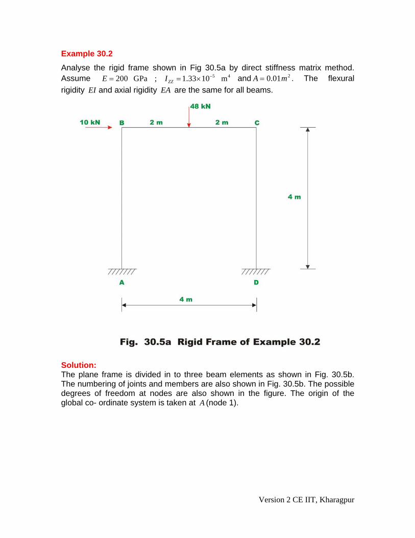
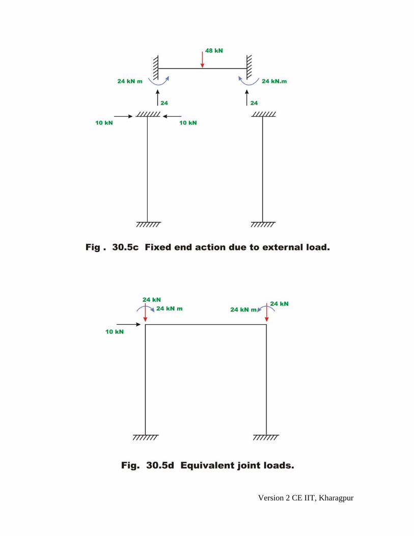
Example 30.2 Analyse the rigid frame shown in Fig 30.5a by direct stiffness matrix method. Assume and . The flexural rigidity

5 4200 GPa ; 1.33 10 mZZE I −= = × 201.0 mA =EI and axial rigidity EA are the same for all beams.

Solution: The plane frame is divided in to three beam elements as shown in Fig. 30.5b. The numbering of joints and members are also shown in Fig. 30.5b. The possible degrees of freedom at nodes are also shown in the figure. The origin of the global co- ordinate system is taken at A (node 1).


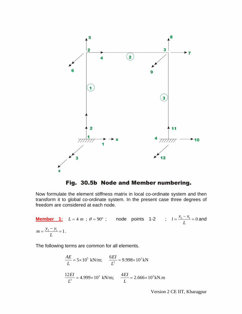
Now formulate the element stiffness matrix in local co-ordinate system and then transform it to global co-ordinate system. In the present case three degrees of freedom are considered at each node.

Member 1: °== 90;4 θmL ; node points 1-2 ; 2 1 0x xlL−

= = and

2 1 1y ymL−

= = .

The following terms are common for all elements.

5 22

65 10 kN/m; 9.998 10 kNAE EIL L

= × = ×

2 3

3

12 44.999 10 kN/m; 2.666 10 kN.mEI EIL L

= × = ×


[ ] [ ] [ ][ ]

6

5

4

3

2

1

1066.201011033.10101

0105001050

10101050.010101050.0

1033.101011066.20101

0105001050

10101050.010101050.0654321

'

3333

55

3333

3333

55

3333

1

⎥⎥⎥⎥⎥⎥⎥⎥⎥⎥

⎦

⎤

⎢⎢⎢⎢⎢⎢⎢⎢⎢⎢

⎣

⎡

××××−

××−

××××−

××××−

×−×

×−×−×−×

=

= TkTk T

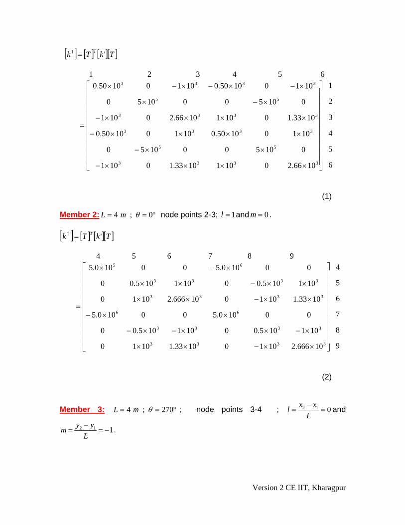
(1) Member 2: °== 0;4 θmL node points 2-3; 1=l and 0=m . [ ] [ ] [ ][ ]

9

8

7

6

5

4

10666.210101033.11010

101105.00101105.00

00100.500100.5

1033.1101010666.21010

101105.00101105.00

00100.500100.5987654

'

3333

3333

66

3333

3333

65

2

⎥⎥⎥⎥⎥⎥⎥⎥⎥⎥

⎦

⎤

⎢⎢⎢⎢⎢⎢⎢⎢⎢⎢

⎣

⎡

××−××

×−××−×−

××−

××−××

××−××

×−×

=

= TkTk T

(2)

Member 3: °== 270;4 θmL ; node points 3-4 ; 2 1 0x xlL−

= = and

2 1 1y ymL−

= = − .


[ ] [ ] [ ][ ]

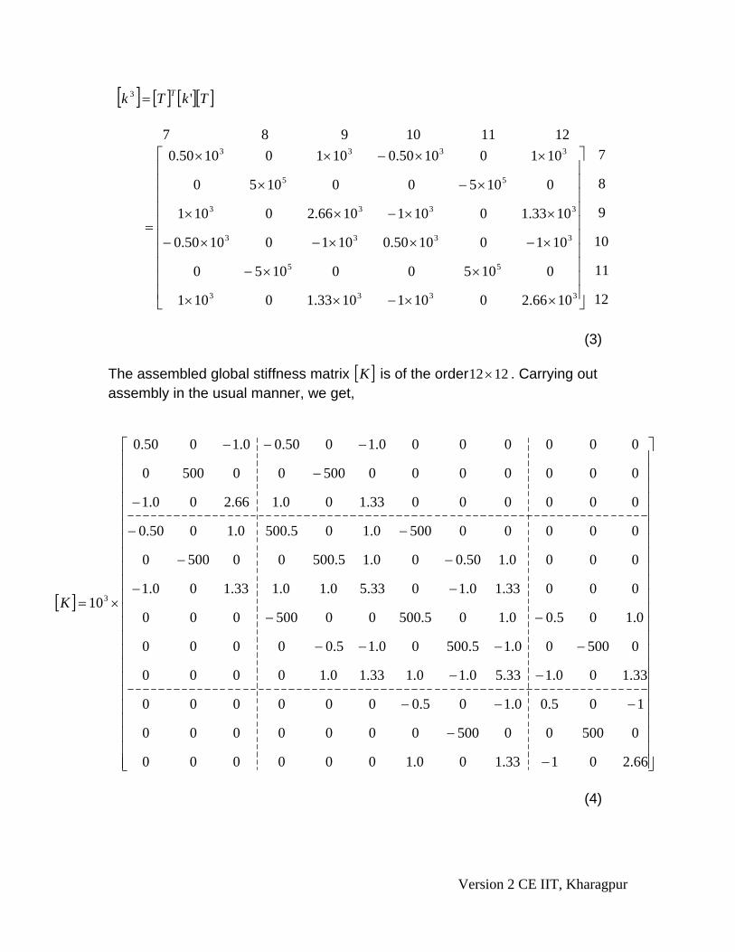
12

11

10

9

8

7

1066.201011033.10101

0105001050

10101050.010101050.0

1033.101011066.20101

0105001050

10101050.010101050.0121110987

'

3333

55

3333

3333

55

3333

3

⎥⎥⎥⎥⎥⎥⎥⎥⎥⎥

⎦

⎤

⎢⎢⎢⎢⎢⎢⎢⎢⎢⎢

⎣

⎡

××−××

××−

×−××−×−

××−××

×−×

××−××

=

= TkTk T

(3) The assembled global stiffness matrix [ ]K is of the order 1212× . Carrying out assembly in the usual manner, we get,

[ ]

⎥⎥⎥⎥⎥⎥⎥⎥⎥⎥⎥⎥⎥⎥⎥⎥⎥⎥⎥⎥⎥⎥⎥

⎦

⎤

⎢⎢⎢⎢⎢⎢⎢⎢⎢⎢⎢⎢⎢⎢⎢⎢⎢⎢⎢⎢⎢⎢⎢

⎣

⎡

−

−

−−−

−−

−−−−

−−

−−

−−

−−

−

−

−−−

×=

66.20133.100.1000000

0500005000000000

105.00.105.0000000

33.100.133.50.10.133.10.10000

050000.15.50000.15.00000

0.105.00.105.50000500000

00033.10.1033.50.10.133.100.1

0000.150.000.15.500005000

000005000.105.5000.1050.0

00000033.100.166.200.1

0000000500005000

0000000.1050.00.1050.0

103K

(4)



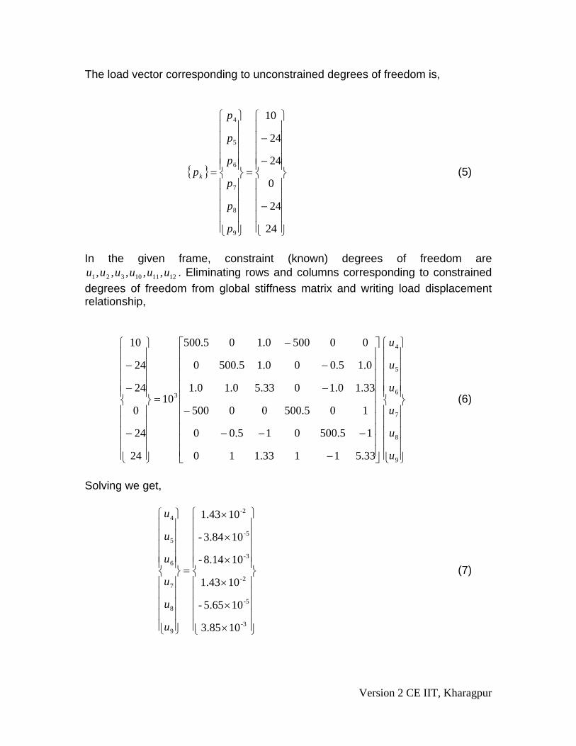
The load vector corresponding to unconstrained degrees of freedom is,

{ }

⎪⎪⎪⎪⎪

⎭

⎪⎪⎪⎪⎪

⎬

⎫

⎪⎪⎪⎪⎪

⎩

⎪⎪⎪⎪⎪

⎨

⎧

−

−

−

=

⎪⎪⎪⎪⎪

⎭

⎪⎪⎪⎪⎪

⎬

⎫

⎪⎪⎪⎪⎪

⎩

⎪⎪⎪⎪⎪

⎨

⎧

=

24

24

0

24

24

10

9

8

7

6

5

4

p

p

p

p

p

p

pk (5)

In the given frame, constraint (known) degrees of freedom are

. Eliminating rows and columns corresponding to constrained degrees of freedom from global stiffness matrix and writing load displacement relationship,

121110321 ,,,,, uuuuuu

⎪⎪⎪⎪⎪

⎭

⎪⎪⎪⎪⎪

⎬

⎫

⎪⎪⎪⎪⎪

⎩

⎪⎪⎪⎪⎪

⎨

⎧

⎥⎥⎥⎥⎥⎥⎥⎥⎥⎥

⎦

⎤

⎢⎢⎢⎢⎢⎢⎢⎢⎢⎢

⎣

⎡

−

−−−

−

−

−

−

=

⎪⎪⎪⎪⎪

⎭

⎪⎪⎪⎪⎪

⎬

⎫

⎪⎪⎪⎪⎪

⎩

⎪⎪⎪⎪⎪

⎨

⎧

−

−

−

9

8

7

6

5

4

3

33.51133.110

15.500015.00

105.50000500

33.10.1033.50.10.1

0.15.000.15.5000

005000.105.500

10

24

24

0

24

24

10

u

u

u

u

u

u

(6)

Solving we get,

⎪⎪⎪⎪⎪

⎭

⎪⎪⎪⎪⎪

⎬

⎫

⎪⎪⎪⎪⎪

⎩

⎪⎪⎪⎪⎪

⎨

⎧

×

×

×

×

×

×

=

⎪⎪⎪⎪⎪

⎭

⎪⎪⎪⎪⎪

⎬

⎫

⎪⎪⎪⎪⎪

⎩

⎪⎪⎪⎪⎪

⎨

⎧

3-

5-

2-

3-

5-

-2

9

8

7

6

5

4

103.85

105.65-

101.43

108.14-

103.84-

1043.1

u

u

u

u

u

u

(7)


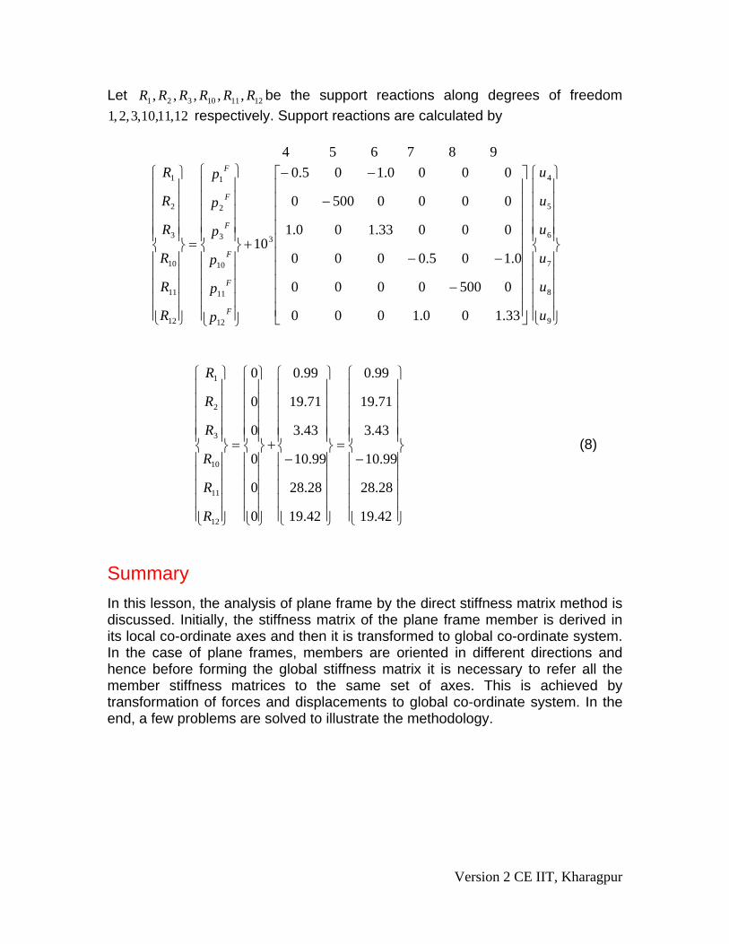
Let be the support reactions along degrees of freedom respectively. Support reactions are calculated by

121110321 ,,,,, RRRRRR12,11,10,3,2,1

⎪⎪⎪⎪⎪

⎭

⎪⎪⎪⎪⎪

⎬

⎫

⎪⎪⎪⎪⎪

⎩

⎪⎪⎪⎪⎪

⎨

⎧

⎥⎥⎥⎥⎥⎥⎥⎥⎥⎥

⎦

⎤

⎢⎢⎢⎢⎢⎢⎢⎢⎢⎢

⎣

⎡

−

−−

−

−−

+

⎪⎪⎪⎪⎪

⎭

⎪⎪⎪⎪⎪

⎬

⎫

⎪⎪⎪⎪⎪

⎩

⎪⎪⎪⎪⎪

⎨

⎧

=

⎪⎪⎪⎪⎪

⎭

⎪⎪⎪⎪⎪

⎬

⎫

⎪⎪⎪⎪⎪

⎩

⎪⎪⎪⎪⎪

⎨

⎧

9

8

7

6

5

4

3

12

11

10

3

2

1

12

11

10

3

2

1

33.100.1000

05000000

0.105.0000

00033.100.1

00005000

0000.105.0

10

987654

u

u

u

u

u

u

p

p

p

p

p

p

R

R

R

R

R

R

F

F

F

F

F

F

⎪⎪⎪⎪⎪

⎭

⎪⎪⎪⎪⎪

⎬

⎫

⎪⎪⎪⎪⎪

⎩

⎪⎪⎪⎪⎪

⎨

⎧

−=

⎪⎪⎪⎪⎪

⎭

⎪⎪⎪⎪⎪

⎬

⎫

⎪⎪⎪⎪⎪

⎩

⎪⎪⎪⎪⎪

⎨

⎧

−+

⎪⎪⎪⎪⎪

⎭

⎪⎪⎪⎪⎪

⎬

⎫

⎪⎪⎪⎪⎪

⎩

⎪⎪⎪⎪⎪

⎨

⎧

=

⎪⎪⎪⎪⎪

⎭

⎪⎪⎪⎪⎪

⎬

⎫

⎪⎪⎪⎪⎪

⎩

⎪⎪⎪⎪⎪

⎨

⎧

42.19

28.28

99.10

43.3

71.19

99.0

42.19

28.28

99.10

43.3

71.19

99.0

0

0

0

0

0

0

12

11

10

3

2

1

R

R

R

R

R

R

(8)

Summary In this lesson, the analysis of plane frame by the direct stiffness matrix method is discussed. Initially, the stiffness matrix of the plane frame member is derived in its local co-ordinate axes and then it is transformed to global co-ordinate system. In the case of plane frames, members are oriented in different directions and hence before forming the global stiffness matrix it is necessary to refer all the member stiffness matrices to the same set of axes. This is achieved by transformation of forces and displacements to global co-ordinate system. In the end, a few problems are solved to illustrate the methodology.


Documents

Lesson 29: Analysis of plane frame by stiffness methodnptel.ac.in/courses/Webcourse-contents/IIT Kharagpur...Instructional Objectives After reading this chapter the student will be