Lectures on Electric-Magnetic Duality and the

Geometric Langlands Program

Anton KapustinCalifornia Institute of Technology, Pasadena, CA 91125, U.S.A.

January 1, 2008

Abstract

These lecture notes are based on the master class given at the Cen-ter for the Topology and Quantization of Moduli Spaces, Universityof Aarhus, August 2007. I provide an introduction to the recent workon the Montonen-Olive duality of N = 4 super-Yang-Mills theory andthe Geometric Langlands Program.

1

1 Introduction

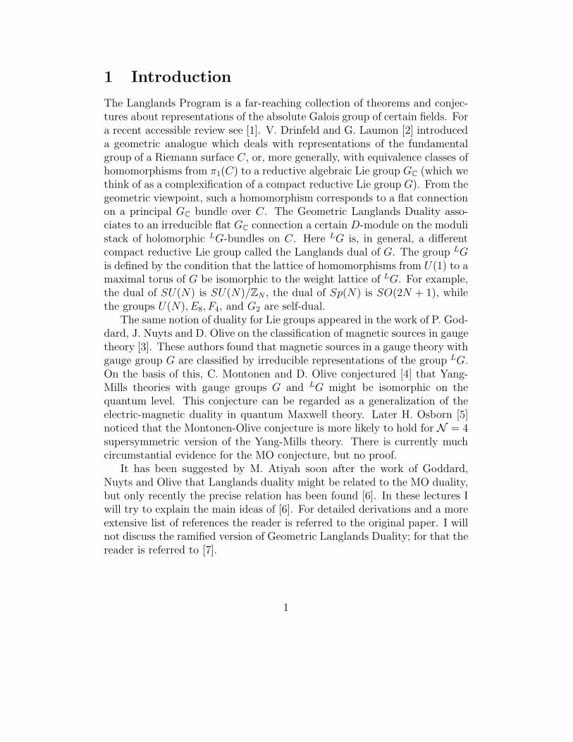
The Langlands Program is a far-reaching collection of theorems and conjec-tures about representations of the absolute Galois group of certain fields. Fora recent accessible review see [1]. V. Drinfeld and G. Laumon [2] introduceda geometric analogue which deals with representations of the fundamentalgroup of a Riemann surface C, or, more generally, with equivalence classes ofhomomorphisms from π1(C) to a reductive algebraic Lie group GC (which wethink of as a complexification of a compact reductive Lie group G). From thegeometric viewpoint, such a homomorphism corresponds to a flat connectionon a principal GC bundle over C. The Geometric Langlands Duality asso-ciates to an irreducible flat GC connection a certain D-module on the modulistack of holomorphic LG-bundles on C. Here LG is, in general, a differentcompact reductive Lie group called the Langlands dual of G. The group LGis defined by the condition that the lattice of homomorphisms from U(1) to amaximal torus of G be isomorphic to the weight lattice of LG. For example,the dual of SU(N) is SU(N)/ZN , the dual of Sp(N) is SO(2N + 1), whilethe groups U(N), E8, F4, and G2 are self-dual.

The same notion of duality for Lie groups appeared in the work of P. God-dard, J. Nuyts and D. Olive on the classification of magnetic sources in gaugetheory [3]. These authors found that magnetic sources in a gauge theory withgauge group G are classified by irreducible representations of the group LG.On the basis of this, C. Montonen and D. Olive conjectured [4] that Yang-Mills theories with gauge groups G and LG might be isomorphic on thequantum level. This conjecture can be regarded as a generalization of theelectric-magnetic duality in quantum Maxwell theory. Later H. Osborn [5]noticed that the Montonen-Olive conjecture is more likely to hold for N = 4supersymmetric version of the Yang-Mills theory. There is currently muchcircumstantial evidence for the MO conjecture, but no proof.

It has been suggested by M. Atiyah soon after the work of Goddard,Nuyts and Olive that Langlands duality might be related to the MO duality,but only recently the precise relation has been found [6]. In these lectures Iwill try to explain the main ideas of [6]. For detailed derivations and a moreextensive list of references the reader is referred to the original paper. I willnot discuss the ramified version of Geometric Langlands Duality; for that thereader is referred to [7].

1

2 Electric-magnetic duality in abelian gauge

theory

I will begin by reviewing electric-magnetic duality in Maxwell theory, whichis a theory of a U(1) gauge field without sources. On the classical level,this theory describes a connection A on a principal U(1) bundle E overa four-manifold X. The four-manifold X is assumed to be equipped with aLorenzian metric (later we will switch to Riemannian metric). The equationsof motion for A read

d ⋆ F = 0,

where F = dA is the curvature of A and ⋆ is the Hodge star operator onforms. In addition, the curvature 2-form F is closed, dF = 0 (this is knownas the Bianchi identity), so one can to a large extent eliminate A in favorF . More precisely, F determines the holonomy of A around all contractibleloops in X. If π1(X) is trivial, F completely determines A, up to gaugeequivalence. In addition, if H2(X) 6= 0, F satisfies a quantization condition:its periods are integral multiples of 2π. The cohomology class of F is theEuler class of E (or alternatively the first Chern class of the associated linebundle).

When X = R3,1, the theory is clearly invariant under a transformation

F 7→ F ′ = ⋆F. (1)

If X is Lorenzian, this transformation squares to −1. It is known as theelectric-magnetic duality. To understand why, let x0 be the time-like coordi-nate and xi, i = 1, 2, 3 be space-like coordinates. Then the usual electric andmagnetic fields are

Ei = F0i, Bi =1

2ǫijkFjk,

and the transformation (1) acts by

Ei 7→ Bi, Bi 7→ −Ei.

Thus, up to some minus signs, the duality transformation exchanges electricand magnetic fields. The signs are needed for compatibility with Lorenztransformations. Alternatively, from the point of view of the Hamiltonianformalism the signs are needed to preserve the symplectic structure on the

2

space of fields Ei and Bi. This symplectic structure corresponds to thePoisson bracket

Bi(x), Ek(y) =e2

2ǫijk∂jδ

3(x− y),

where e2 is the coupling constant (it determines the overall normalization ofthe action).

As remarked above, the classical theory can be rewritten entirely in termsof F only on simply-connected manifolds. In addition, the ⋆F need not satisfyany quantization condition, unlike F . Thus it appears that on manifolds morecomplicated than R3,1 the duality is absent. Interestingly, in the quantumtheory the duality is restored for any X, if one sums over all topologies ofthe bundle E. To see how this comes about, let us recall that the quantumtheory is defined by its path-integral

Z =

∫

DA eiS(A),

where S(A) is the action functional. We take the action to be

S(A) =1

2e2

∫

X

F ∧ ⋆F +θ

8π2

∫

X

F ∧ F.

Its critical points are precisely solutions of d ⋆ F = 0. Note that the secondterm in the action depends only on the topology of E and therefore does notaffect the classical equations of motion. But it does affect the action andtherefore has to be considered in the quantum theory. In fact, if we sum overall isomorphism classes of E, i.e. define the path-integral as

Z =∑

E

∫

DA eiS(A),

the parameter θ tells us how to weigh contributions of different E.At this stage it is very convenient to replace X with a Riemannian man-

ifold (which we will also denote X). The idea here is that the path-integralfor a Lorenzian manifold should be defined as an analytic continuation of thepath-integral in Euclidean signature; this is known as the Wick rotation. InEuclidean signature the path-integral and the action look slightly different:

Z =∑

E

∫

DA e−SE(A),

3

where

SE(A) =

∫

X

(

1

2e2F ∧ ⋆F −

iθ

8π2F ∧ F

)

Note that the action becomes complex in Euclidean signature.Now let us sketch how duality arises on the quantum level. Assuming

that X is simply-connected for simplicity, we can replace integration over Awith integration over the space of closed 2-forms F satisfying the quantiza-tion condition on periods. If we further assume X = R4, the quantizationcondition is empty, and the partition function can be written as

Z =

∫

DFDB exp

(

−SE + i

∫

X

B ∧ dF

)

.

Here the new field B is a 1-form on X introduced so that integration overit produces the delta-functional δ(dF ) =

∏

x∈X δ(dF (x)). This allows us tointegrate over all (not necessarily closed) 2-forms F .

Now we can do the integral over F using the fact that it is a Gaussianintegral. The result is

Z =

∫

DB exp

(

−1

2e2

∫

X

G ∧ ⋆G+iθ

8π2

∫

X

G ∧G

)

,

where G = dB, and the parameters e2 and θ are defined by

θ

2π+

2πi

e2= −

(

θ

2π+

2πi

e2

)−1

.

We see that the partition function written as an integral over B has exactlythe same form as the partition function written as an integral over A, butwith e2 and θ replaced with e2 and θ. This is a manifestation of electric-magnetic duality. To see this more clearly, note that for θ = 0 the equationsof motion for F deduced from the action

SE(F ) − i

∫

X

B ∧ dF

readsF = ie2 ⋆ G.

4

The factor i arises because of Riemannian signature of the metric; in Loren-zian signature similar manipulations would produce an identical formula butwithout i.

The above derivation of electric-magnetic duality is valid only when Xis topologically trivial. If H2(X) 6= 0, we have to insert additional delta-functions in the path-integral for F and B ensuring that the periods of Fare properly quantized. It turns out that the effect of these delta-functionscan be reproduced by letting B to be a connection 1-form on an arbitraryprincipal U(1) bundle E over X and summing over all possible E. For aproof valid for general 4-manifolds X see [8].

We see from this derivation that duality acts nontrivially on the couplinge2 and the parameter θ. To describe this action, it is convenient to introducea complex parameter τ taking values in the upper half-plane:

τ =θ

2π+

2πi

e2.

Then electric-magnetic duality acts by

τ → −1/τ.

Note that the transformation τ → τ+1 or equivalently the shift θ → θ+2πis also a symmetry of the theory if X is spin. Indeed, θ enters the action asthe coefficient of the topological term

−i

2c21,

where c1 is the first Chern class of E. If X is spin, the square of any integralcohomology class is divisible by two, and so the above topological term isi times an integer. This immediately implies that shifting θ by 2π leavese−SE unchanged. (For arbitrary X the transformation τ → τ + 2 is still asymmetry.)

The transformations τ → −1/τ and τ → τ + 1 generated the wholegroup of integral fractional-linear transformations acting on the upper half-plane, i.e. the group PSL(2,Z). Points in the upper half-plane related bythe PSL(2,Z) give rise to isomorphic theories. One may call this groupthe duality group. Actually, it is better to reserve this name for its “double-cover” SL(2,Z), since applying the electric-magnetic duality twice acts by −1on the 2-form F . In this lectures we will mostly focus on electric-magnetic

5

duality, which is a particular element of SL(2,Z). It is also known as S-duality. Note that for θ = 0 S-duality exchanges weak coupling (e2 ≪ 1) andstrong coupling (e2 ≫ 1). This does not cause problems in the abelian case,because we can solve the U(1) gauge theory for any value of the coupling.But it will greatly complicate the matters in the nonabelian case, where thetheory is only soluble for small e2.

3 Montonen-Olive Duality

Now let us try to generalize the above considerations to a nonabelian gaugetheory, also known as Yang-Mills theory. The basic field is a connectionA = Aµdx

µ on a principal G-bundle E over a four-dimensional manifoldX. The four-manifold X is equipped with a Lorenzian metric g, and theequations of motion read

dAF = 0, dA ⋆ F = 0,

where F = dA + A ∧ A ∈ Ω2(ad(E)) is the curvature of A, dA is the covari-ant differential, and ⋆ is the Hodge star operator on X. The first of theseequations is satisfied identically, while the second one follows from varyingthe Yang-Mills action

S(A) =

∫

X

(

1

2e2TrF ∧ ⋆F +

θ

8π2TrF ∧ F

)

The corresponding Euclidean action is

SE(A) =

∫

X

(

1

2e2TrF ∧ ⋆F − i

θ

8π2TrF ∧ F

)

The action has two real parameters, e and θ. Neither of them affects theclassical equations of motion, but they do affect the quantized Yang-Millstheory. On the quantum level one should consider a path integral

Z =∑

E

∫

DA e−SE(A), (2)

and it does depend on both e and θ.

6

For each X the path-integral (2) is a single function of e2 and θ and sois not very informative (it is known as the partition function of Yang-Millstheory). More generally, one can consider path-integrals of the form

∑

E

∫

DA e−SE(A)O1(A)O2(A) . . .Ok(A),

where O1, . . . ,Ok are gauge-invariant functions of A called observables. Sucha path-integral is called a correlator of observables O1, . . . ,Ok and denoted

〈O1 . . .Ok〉.

An example of an observable in Yang-Mills theory is

O(A) = WR(γ) = TrR(Holγ(A)),

where γ is a closed curve inX, Holγ(A) is the holonomy of A along γ, and R isan irreducible representation of G. Such observables are called Wilson loops[9]; they play an important role in the geometric Langlands duality, as wewill see below. From the physical viewpoint, inserting WR(γ) into the path-integral corresponds to inserting an electrically charged source (“quark”) inthe representation R whose worldline is γ. In semiclassical Yang-Mills theory,such a source creates a Coulomb-like field of the form

Aa0 = T a e2

4πr

where T a, a = 1, dimG, are generators of G in representation R. Here wetook X = R × R3, r is the distance from the origin in R3, and we assumedthat the worldline of the source is given by r = 0.

In the case G = U(1), we saw that the theory enjoys a symmetry whichin Lorenzian signature acts by

F → F = e2 ⋆ F, τ → τ = −1/τ.

At first sight, it seems unlikely that such a duality could extend to a theorywith a nonabelian gauge group, since equations of motion explicitly dependon A, not just on F . The first hint in favor of a nonabelian generalizationof electric-magnetic duality was the work of Goddard, Nuyts, and Olive [3].They noticed that magnetic sources in a nonabelian Yang-Mills theory are

7

labeled by irreducible representations of a different group which they calledthe magnetic gauge group. As a matter of fact, the magnetic gauge groupcoincides with the Langlands dual of G, so we will denote it LG. A staticmagnetic source in Yang-Mills theory should create a field of the form

F = ⋆3 d( µ

2r

)

,

where µ is an element of the Lie algebra g of G defined up to adjoint actionof G, and ⋆3 is the Hodge star operator on R3. Goddard, Nuyts, and Oliveshowed that µ is “quantized”. More precisely, using gauge freedom one canassume that µ lies in a particular Cartan subalgebra t of g, and then it turnsout that µ must lie in the coweight lattice of G, which, by definition, is thesame as the weight lattice of LG.1 Furthermore, µ is defined up to an actionof the Weyl group, so possible values of µ are in one-to-one correspondencewith highest weights of LG.

On the basis of this observation, C. Montonen and D. Olive [4] conjecturedthat Yang-Mills theories with gauge groups G and LG are isomorphic on thequantum level, and that this isomorphism exchanges electric and magneticsources. Thus the Montonen-Olive duality is a nonabelian version of electric-magnetic duality in Maxwell theory.

In order for the energy of electric and magnetic sources to transformproperly under MO duality, one has to assume that for θ = 0 the dual gaugecoupling is

e2 =16π2ng

e2. (3)

Here the integer ng is 1, 2, or 3 depending on the maximal multiplicity ofedges in the Dynkin diagram of g [10, 11]; for simply-laced groups ng = 1.This means that MO duality exchanges weak coupling (e → 0) and strongcoupling (e → ∞). For this reason, it is extremely hard to prove the MOduality conjecture. For general θ, we define

τ =θ

2π+

4πi

e2.

(The slight difference in the definition of τ compared to the nonabelian caseis due to a different normalization of the Killing metric on the Lie algebra.)

1The coweight lattice of G is defined as the lattice of homomorphisms from U(1) to amaximal torus T of G. The weight lattice of G is the lattice of homomorphisms from T

to U(1).

8

The parameter τ takes values in the upper half-plane and under MO dualitytransforms as

τ → τ = −1

ngτ(4)

The Yang-Mills theory has another, much more elementary symmetry,which does not change the gauge group:

τ → τ + k.

Here k is an integer which depends on the geometry ofX andG. For example,if X = R4, then k = 1 for all G. Together with the MO duality, thesetransformations generate some subgroup of SL(2,R). In what follows wewill mostly set θ = 0 and will discuss only the Z4 subgroup generated by theMO duality.

To summarize, if the MO duality were correct, then the partition functionwould satisfy

Z(X,G, τ) = Z(X, LG,−1

ngτ)

Of course, the partition function is not a very interesting observable. Isomor-phism of two quantum field theories means that we should be able to matchall observables in the two theories. That is, for any observable O in the gaugetheory with gauge group G we should be able to construct an observable Oin the gauge theory with gauge group LG so that all correlators agree:

〈O1 . . . On〉X,G,τ = 〈O1 . . . On〉X,LG,−1/(ngτ)

At this point I should come clean and admit that the MO duality asstated above is not correct. The most obvious objection is that the parame-ters e and e are renormalized, and the relation like (3) is not compatible withrenormalization. However, it was pointed out later by Osborn [5] (who wasbuilding on the work of Witten and Olive [12]) that the duality makes muchmore sense in N = 4 super-Yang-Mills theory. This is a maximally super-symmetric extension of Yang-Mills theory in four dimensions, and it has aremarkable property that the gauge coupling is not renormalized at any orderin perturbation theory. Furthermore, Osborn was able to show that certainmagnetically-charged solitons in N = 4 SYM theory have exactly the samequantum numbers as gauge bosons. (The argument assumes that the vac-uum breaks spontaneously the gauge group G down to its maximal abeliansubgroup, so that both magnetically charged solitons and the corresponding

9

gauge bosons are massive). Later strong evidence in favor of the MO dualityfor N = 4 SYM was discovered by A. Sen [13] and C. Vafa and E. Witten[14]. Nowadays MO duality is often regarded as a consequence of string du-alities. One particular derivation which works for all G is explained in [15].Nevertheless, the MO duality is still a conjecture, not a theorem. In whatfollows we will assume its validity and deduce from it the main statementsof the Geometric Langlands Program.

Apart from the connection 1-form A, N = 4 SYM theory contains sixscalar fields φi, i = 1, . . . , 6, which are sections of ad(E), four spinor fieldsλa, a = 1, . . . , 4, which are sections of ad(E) ⊗ S− and four spinor fieldsλa, a = 1, . . . , 4 which are sections of ad(E) ⊗ S+. Here S± are the twospinor bundles over X. The fields A and φi are bosonic (even), while thespinor fields are fermionic (odd). In Minkowski signature the fields λa andλa are complex-conjugate, but in Euclidean signature they are independent.

The action of N = 4 SYM theory has the form

SN=4 = SY M +1

e2

∫

X

(

∑

i

TrDφi ∧ ⋆Dφi + volX∑

i<j

Tr[φi, φj]2

)

+ . . .

where dots denote terms depending on the fermions. The action has Spin(6) ≃SU(4) symmetry under which the scalars φi transform as a vector, the fieldsλa transform as a spinor, and λa transform as the dual spinor. This sym-metry is present for any Riemannian X and is known as the R-symmetry.If X is R4 with a flat metric, the action also has translational and rota-tional symmetries, as well as sixteen supersymmetries Qaα and Qa

α, wherea = 1, . . . , 4 and the Spin(4) spinor indices α and α run from 1 to 2. As isclear from the notation, Qa and Qa transform as spinors and dual spinorsof the R-symmetry group Spin(6); they also transform as spinors and dualspinors of the rotational group Spin(4).

One can show that under the MO duality all bosonic symmetry generatorsare mapped trivially, while supersymmetry generators are multiplied by a τ -dependent phase:

Qa → eiφ/2Qa, Qa → e−iφ/2Qa, eiφ =|τ |

τ

This phase will play an important role in the next section.

10

4 Twisting N = 4 super-Yang-Mills theory

In order to extract mathematical consequences of MO duality, we are goingto turn N = 4 SYM theory into a topological field theory. The procedure fordoing this is called topological twisting [16].

Topological twisting is a two-step procedure. On the first step, onechooses a homomorphism ρ from Spin(4), the universal cover of the structuregroup of TX, to the R-symmetry group Spin(6). This enables one to rede-fine how fields transform under Spin(4). The choice of ρ is constrained bythe requirement that after this redefinition some of supersymmetries becomescalars, i.e. transform trivially under Spin(4). Such supersymmetries survivewhen X is taken to be an arbitrary Riemannian manifold. In contrast, if weconsider ordinary N = 4 SYM on a curved X, it will have supersymmetryonly if X admits a covariantly constant spinor.

It is easy to show that there are three inequivalent choices of ρ satisfy-ing these constraints [14]. The one relevant for the Geometric LanglandsProgram is identifies Spin(4) with the obvious Spin(4) subgroup of Spin(6).After redefining the spins of the fields accordingly, we find that one of theleft-handed supersymmetries and one of the right-handed supersymmetriesbecome scalars. We will denote them Ql and Qr respectively.

On the second step, one notices that Ql and Qr both square to zero andanticommute (up to a gauge transformation). Therefore one may pick anylinear combination of Ql and Qr

Q = uQl + vQr,

and declare it to be a BRST operator. That is, one considers only observableswhich are annihilated by Q (and are gauge-invariant) modulo those whichare Q-exact. This is consistent because any correlator involving Q-closedobservables, one of which is Q-exact, vanishes. From now on, all observablesare assumed to be Q-closed. Correlators of such observables will be calledtopological correlators.

Clearly, the theory depends on the complex numbers u, v only up to anoverall scaling. Thus we get a family of twisted theories parameterized bythe projective line P1. Instead of the homogenous coordinates u, v, we willmostly use the affine coordinate t = v/u which takes values in C ∪ ∞.All these theories are diffeomorphism-invariant, i.e. do not depend on theRiemannian metric. To see this, one writes an action (which is independent

11

of t) in the form

I = Q, V +iΨ

4π

∫

X

TrF ∧ F

where V is a gauge-invariant function of the fields, and Ψ is given by

Ψ =θ

2π+t2 − 1

t2 + 1

4πi

e2

All the metric dependence is in V , and since changing V changes the actionby Q-exact terms, we conclude that topological correlators are independentof the metric.

It is also apparent that for fixed t topological correlators are holomorphicfunctions of Ψ, and this dependence is the only way e2 and θ may enter. Inparticular, for t = i we have Ψ = ∞, independently of e2 and θ. This meansthat for t = i topological correlators are independent of e2 and θ.

To proceed further, we need to describe the field content of the twistedtheory. Since the gauge field A is invariant under Spin(6) transformations,it is not affected by the twist. As for the scalars, four of them becomecomponents of a 1-form φ with values in ad(E), and the other two remainsections of ad(E); we may combine the latter into a complex scalar field σwhich is a section of the complexification of ad(E). The fermionic fields inthe twisted theory are a pair of 1-forms ψ and ψ, a pair of 0-forms η and η,and a 2-form χ, all taking values in the complexification of ad(E).

What makes the twisted theory manageable is that the path integral lo-calizes on Q-invariant field configurations. One way to deduce this propertyis to note that as a consequence of metric-independence, semiclassical (WKB)approximation is exact in the twisted theory. Thus the path-integral local-izes on absolute minima of the Euclidean action. On the other hand, suchconfigurations are exactly Q-invariant configurations.

The condition of Q-invariance is a set of partial differential equations onthe bosonic fields A, φ and σ. We will only state the equations for A and φ,since the equations for σ generically imply that σ = 0:

(F − φ ∧ φ+ tDφ)+ = 0, (F − φ ∧ φ− t−1Dφ)− = 0, D ⋆ φ = 0. (5)

Here subscripts + and − denote self-dual and anti-self-dual parts of a 2-form.If t is real, these equations are elliptic. A case which will be of special

interest is t = 1; in this case the equations can be rewritten as

F − φ ∧ φ+ ⋆Dφ = 0, D ⋆ φ = 0.

12

They resemble both the Hitchin equations in 2d [17] and the Bogomolny equa-tions in 3d [18] (and reduce to them in special cases). The virtual dimensionof the moduli space of these equations is zero, so the partition function is theonly nontrivial observable if X is compact without boundary. However, forapplications to the Geometric Langlands Program it is important to considerX which are noncompact and/or have boundaries.

Another interesting case is t = i. To understand this case, it is conve-nient to introduce a complex connection A = A+ iφ and the correspondingcurvature F = dA + A2. Then the equations are equivalent to

F = 0, D ⋆ φ = 0.

The first of these equations is invariant under the complexified gauge trans-formations, while the second one is not. It turns out that the moduli spaceis unchanged if one drops the second equation and considers the space ofsolutions of the equation F = 0 modulo GC gauge transformations. Moreprecisely, according to a theorem of K. Corlette [19], the quotient by GC

gauge transformations should be understood in the sense of Geometric In-variant Theory, i.e. one should distinguish stable and semistable solutions ofF = 0 and impose a certain equivalence relation on semistable solutions. Theresulting moduli space is called the moduli space of stable GC connections onX and will be denoted Mflat(G,X). Thus for t = i the path integral of thetwisted theory reduces to an integral over Mflat(G,X). This is an indicationthat twisted N = 4 SYM with gauge group G has something to do with thestudy of homomorphisms from π1(X) to GC.

Finally, let us discuss how MO duality acts on the twisted theory. The keyobservation is that MO duality multiplies Ql and Qr by e±iφ/2, and thereforemultiplies t by a phase:

t 7→|τ |

τt.

Since Imτ 6= 0, the only points of the P1 invariant under the MO dualityare the “poles” t = 0 and t = ∞. On the other hand, if we take t = i andθ = 0, then the MO duality maps it to a theory with t = 1 and θ = 0 (it alsoreplaces G with LG). As we will explain below, it is this special case of theMO duality that gives rise to the Geometric Langlands Duality.

13

5 Reduction to two dimensions

From now on we specialize to the case X = Σ × C where C and Σ areRiemann surfaces. We will assume that C has no boundary and has genusg > 1, while Σ may have a boundary. In our discussion we will mostly worklocally on Σ, and its global structure will be unimportant.

Topological correlators are independent of the volumes of C and Σ. How-ever, to exploit localization, it is convenient to consider the limit in whichthe volume of C goes to zero. In the spirit of the Kaluza-Klein reduction,we expect that in this limit the 4d theory becomes equivalent to a 2d the-ory on Σ. In the untwisted theory, this equivalence holds only in the limitvol(C) → 0, but in the twisted theory the equivalence holds for any volume.

It is easy to guess the effective field theory on Σ. One begins by consider-ing the case Σ = R2 and requiring the field configuration to be independentof the coordinates on Σ and to have zero energy. On can show that a genericsuch configuration has σ = 0, while φ and A are pulled-back from C andsatisfy

F − φ ∧ φ = 0, Dφ = 0, D ⋆ φ = 0.

Here all quantities as well as the Hodge star operator refer to objects livingon C. These equations are known as Hitchin equations [17], and their spaceof solutions modulo gauge transformations is called the Hitchin moduli spaceMH(G,C). The space MH(G,C) is a noncompact manifold of dimension4(g − 1) dimG with singularities.2 From the physical viewpoint, MH(G,C)is the space of classical vacua of the twisted N = 4 SYM on C × R2.

In the twisted theory, only configurations with vanishingly small energiescontribute. In the limit vol(C) → 0, such configurations will be representedby slowly varying maps from Σ to MH(G,C). Therefore we expect the effec-tive field theory on Σ to be a topological sigma-model with target MH(G,C).

Before we proceed to identify more precisely this topological sigma-model,let us note that MH(G,C) has singularities coming from solutions of Hitchinequations which are invariant under a subgroup of gauge transformations. Inthe neighborhood of such a classical vacuum, the effective field theory is notequivalent to a sigma-model, because of unbroken gauge symmetry. In fact,it is difficult to describe the physics around such vacua in purely 2d terms.We will avoid this difficulty by imposing suitable conditions on the boundaryof Σ ensuring that we stay away from such dangerous points.

2We assumed g > 1 precisely to ensure that virtual dimension of MH(G, C) is positive.

14

The most familiar examples of topological sigma-models are A and B-models associated to a Calabi-Yau manifold M [20]. Both models are ob-tained by twisting a supersymmetric sigma-model with target M . The path-integral of the A-model localizes on holomorphic maps from Σ to M andcomputes the Gromov-Witten invariants of M . The path-integral for theB-model localizes on constant maps to M and can be interpreted mathemat-ically in terms of deformation theory of M regarded as a complex manifold[21]. Both models are topological field theories (TFTs), in the sense thatcorrelators do not depend on the metric on Σ. In addition, the A-modeldepends on the symplectic structure of M , but not on its complex structure,while the B-model depends on the complex structure of M , but not on itssymplectic structure.

As explained above, we expect that our family of 4d TFTs, when consid-ered on a 4-manifold of the form Σ × C, becomes equivalent to a family oftopological sigma-models with target MH(G,C). To connect this family toordinary A and B-models, we note that MH(G,C) is a (noncompact) hyper-Kahler manifold. That is, it has a P1 worth of complex structures compatiblewith a certain metric. This metric has the form

ds2 =1

e2

∫

C

Tr (δA ∧ ⋆δA+ δφ ∧ ⋆δφ)

where (δA, δφ) is a solution of the linearized Hitchin equations representinga tangent vector to MH(G,C).3 If we parameterize the sphere of complexstructures by a parameter w ∈ C∪∞, the basis of holomorphic differentialsis

δAz − w δφz, δAz + w−1δφz.

By varying w, we get a family of B-models with target MH(G,C). Similarly,since for each w we have the corresponding Kahler form on MH(G,C), byvarying w we get a family of A-models with target MH(G,C). However, thefamily of topological sigma-models obtained from the twisted N = 4 SYMdoes not coincide with either of these families. The reason for this is that ageneric A-model or B-model with target MH(G,C) depends on the complexstructure on C, and therefore cannot arise from a TFT on Σ × C.

As explained in [6], this puzzle is resolved by recalling that for a hyper-Kahler manifold M there are twists other than ordinary A or B twists. In

3The overall normalization of the metric we use is natural from the point of view ofgauge theory.

15

general, twisting a supersymmetric sigma-model requires picking two com-plex structures on the target. If we are given a Kahler structure on M , onecan choose the two complex structures to be the same (B-twist) or opposite(A-twist). But for a hyper-Kahler manifold there is a whole sphere of com-plex structures, and by independently varying the two complex structuresone gets P1 ×P1 worth of 2d TFTs. They are known as generalized topolog-ical sigma-models, since their correlators depend on a generalized complexstructure on the target M [22, 23]. The notion of a generalized complexstructure was introduced by N. Hitchin [24] and it includes complex andsymplectic structures are special cases.

It turns out that for M = MH(G,C) there is a 1-parameter subfamily ofthis 2-parameter family of topological sigma-models which does not dependon the complex structure or Kahler form of C. It is this subfamily whichappears as a reduction of the twisted N = 4 SYM theory. Specifically, thetwo complex structures on MH(G,C) are given by

w+ = −t, w− = t−1

Note that one gets a B-model if and only if w+ = w−, i.e. if t = ±i. Onegets an A-model if and only if t is real. All other values of t correspond togeneralized topological sigma-models.

Luckily to understand Geometric Langlands Duality we mainly need thetwo special cases t = i and t = 1. The value t = i corresponds to a B-modelwith complex structure J defined by complex coordinates

Az + iφz, Az + iφz

on MH(G,C). These are simply components of the complex connectionA = A + iφ along C. In terms of this complex connection two out of threeHitchin equations are equivalent to

F = dA + A2 = 0

This equation is invariant under complexified gauge transformations. Thethird equation D ⋆ φ = 0 is invariant only under G gauge transformations.By a theorem of S. Donaldson [25], one can drop this equation at the expenseof enlarging the gauge group from G to GC.(More precisely, one also has toidentify certain semistable solutions of the equation F = 0.) This is analo-gous to the situation in four dimensions. Thus in complex structure J the

16

moduli space MH(G,C) can be identified with the moduli space Mflat(G,C)of stable flat GC connections on C. It is apparent that J is independent ofthe complex structure on C, which implies that the B-model at t = i is alsoindependent of it.

The value t = 1 corresponds to an A-model with a symplectic structureω = 4πωK/e

2, where

ωK = −1

2π

∫

C

Tr δφ ∧ δA.

It is a Kahler form of a certain complex structure K on MH(G,C). Notethat ωK is exact and independent of the complex structure on C.

Yet another complex structure on MH(G,C) is I = JK. It will makean appearance later, when we discuss Homological Mirror Symmetry forMH(G,C). In this complex structure, MH(G,C) can be identified with themoduli space of stable holomorphic Higgs bundles. Recall that a (holomor-phic) Higgs bundle over C (with gauge group G) is a holomorphic G-bundleE over C together with a holomorphic section ϕ of ad(E). In complex di-mension one, any principal G bundle can be thought of as a holomorphicbundle, and Hitchin equations imply that ϕ = φ1,0 satisfies

∂ϕ = 0.

This gives a map from MH(G,C) to the set of gauge-equivalence classesof Higgs bundles. This map becomes one-to-one if we limit ourselves tostable or semistable Higgs bundles and impose a suitable equivalence rela-tionship on semistable ones. This gives an isomorphism between MH(G,C)and MHiggs(G,C).

It is evident that the complex structure I, unlike J , does depend on thechoice of complex structure on C. Therefore the B-model for the modulispace of stable Higgs bundles cannot be obtained as a reduction of a 4dTFT.4 On the other hand, the A-model for MHiggs(G,C) is independent ofthe choice of complex structure on C, because the Kahler form ωI is givenby

ωI =1

4π

∫

C

Tr (δA ∧ δA− δφ ∧ δφ).

In fact, the A-model for MHiggs(G,C) is obtained by letting t = 0. Thisspecial case of reduction to 2d has been first discussed in [27].

4It can be obtained as a reduction of a “holomorphic-topological” gauge theory onΣ × C [26].

17

6 Mirror Symmetry for the Hitchin moduli

space

Now we are ready to infer the consequences of the MO duality for the topo-logical sigma-model with target MH(G,C). For θ = 0, the MO dualityidentifies twisted N = 4 SYM theory with gauge group LG and t = i witha similar theory with gauge group G and t = 1. Therefore the B-modelwith target Mflat(

LG,C) and the A-model with target (M(G,C), ωK) areisomorphic.

Whenever we have two Calabi-Yau manifolds M and M ′ such that theA-model of M is equivalent to the B-model of M ′, we say that M and M ′ area mirror pair. Thus MO duality implies that Mflat(

LG,C) and MH(G,C)(with the symplectic structure ωK) are a mirror pair. This mirror symmetrywas first proposed in [28].

The most obvious mathematical interpretation of this statement involvesthe isomorphism of two Frobenius manifolds associated to the A-model of(MH(G,C), ωK) and the B-model of Mflat(

LG,C). The former of theseencodes the Gromov-Witten invariants of MH(G,C), while the latter onehas to to with the complex structure deformations of Mflat(

LG,C). But onecan get a much stronger statement by considering the categories of topologicalD-branes associated to the two models.

Recall that a topological D-brane for a 2d TFT is a BRST-invariantboundary condition for it. The set of all topological D-branes has a naturalstructure of a category (actually, an A∞ category). For a B-model witha Calabi-Yau target M , this category is believed to be equivalent to thederived category of coherent sheaves on M . Sometimes we will also refer toit as the category of B-branes on M . For an A-model with target M ′, weget a category of A-branes on M ′. It contains the derived Fukaya categoryof M ′ as a full subcategory. For a review of these matters, see e.g. [29].

It has been argued by A. Strominger, S-T. Yau and E. Zaslow (SYZ)[30] that whenever M and M ′ are mirror to each other, they should admitLagrangian torus fibrations over the same base B, and these fibrations aredual to each other, in a suitable sense. In the case of Hitchin moduli spaces,the SYZ fibration is easy to identify [6]. One simply maps a solution (A, φ)of the Hitchin equations to the space of gauge-invariant polynomials builtfrom ϕ = φ1,0. For example, for G = SU(N) or G = SU(N)/ZN the algebra

18

of gauge-invariant polynomials is generated by

Pn = Trϕn ∈ H0(C,KnC), n = 2, . . . , N,

so the fibration map maps MH(G,C) to the vector space

⊕Nn=2H

0(C,KnC).

The map is surjective [31], so this vector space is the base space B. The mapto B is known as the Hitchin fibration of MH(G,C). It is holomorphic incomplex structure I and its fibers are Lagrangian in complex structures JandK. In fact, one can regard MHiggs(G,C) as a complex integrable system,in the sense that the generic fiber of the fibration is a complex torus which isLagrangian with respect to a holomorphic symplectic form on MHiggs(G,C)

ΩI = ωJ + iωK .

(Ordinarily, an integrable system is associated with a real symplectic mani-fold with a Lagrangian torus fibration.)

For generalG one can define the Hitchin fibration in a similar way, and onealways finds that the generic fiber is a complex Lagrangian torus. Moreover,the bases B and LB of the Hitchin fibrations for MH(G,C) and MH(LG,C)are naturally identified.5

While the Hitchin fibration is an obvious candidate for the SYZ fibration,can we prove that it really is the SYZ fibration? It turns out this statementcan be deduced from some additional facts about MO duality.

While we do not know how the MO duality acts on general observables inthe twisted theory, the observables Pn are an exception, as their expectationvalues parameterize the moduli space of vacua of the twisted theory on X =R4. The MO duality must identify the moduli spaces of vacua, in a wayconsistent with other symmetries of the theory, and this leads to a uniqueidentification of the algebras generated by Pn for G and LG. See [6] fordetails.

To complete the argument, we need to consider some particular topolog-ical D-branes for MH(G,C) and MH(LG,C). The simplest example of aB-brane on Mflat(

LG,C) is the structure sheaf of a (smooth) point. What isits mirror? Since each point p lies in some fiber LFp of the Hitchin fibration,

5In some cases G and LG coincide, but the relevant identification is not necessarily theidentity map [11, 6].

19

its mirror must be an A-brane on MH(G,C) localized on the correspondingfiber Fp of the Langlands-dual fibration. By definition, this means that theHitchin fibration is the same as the SYZ fibration.

According to Strominger, Yau, and Zaslow, the fibers of the two mirrorfibrations over the same base point are T-dual to each other. Indeed, bythe usual SYZ argument the A-brane on Fp must be a rank-one object ofthe Fukaya category, i.e. a flat unitary rank-1 connection on a topologicallytrivial line bundle over Fp. The moduli space of such objects must coincidewith the moduli space of the mirror B-brane, which is simply LFp. This isprecisely what we mean by saying that that LFp and Fp are T-dual.

In the above discussion we have tacitly assumed that both MH(G,C)and MH(LG,C) are connected. The components of MH(G,C) are labeledby the topological isomorphism classes of principal G-bundles over C, i.e. byelements of H2(C, π1(G)) = π1(G). Thus, strictly speaking, our discussionapplies literally only when both G and LG are simply-connected. This israrely true; for example, among compact simple Lie groups only E8, F4 andG2 satisfy this condition (all these groups are self-dual).

In general, to maintain mirror symmetry between MH(G,C) and MH(LG,C),one has to consider all possible flat B-fields on both manifolds. A flat B-fieldonM is a class inH2(M,U(1)) whose image inH3(M,Z) under the Bocksteinhomomorphism is trivial. In the case of MH(G,C), the allowed flat B-fieldshave finite order; in fact, they take values in H2(C,Z(G)) = Z(G), whereZ(G) is the center of G. It is well known that Z(G) is naturally isomorphicto π1(

LG). One can show that MO duality maps the class w ∈ Z(G) definingthe B-field on MH(G,C) to the corresponding element in π1(

LG) labelingthe connected component of MH(LG,C) (and vice versa). For example, ifG = SU(N), then MH(G,C) is connected and has N possible flat B-fieldslabeled by Z(SU(N)) = ZN . On the other hand, LG = SU(N)/ZN , andtherefore MH(LG,C) has N connected components labeled by π1(

LG) = ZN .There can be no nontrivial flat B-field on MH(LG,C) in this case. See section7 of [6] for more details.

Let us summarize what we have learned so far. MO duality implies thatMH(G,C) and MH(LG,C) are a mirror pair, with the SYZ fibrations beingthe Hitchin fibrations. The most powerful way to formulate the statementof mirror symmetry between two Calabi-Yau manifolds is in terms of thecorresponding categories of topological branes. In the present case, we getthat the derived category of coherent sheaves on Mflat(

LG,C) is equivalentto the category of A-branes on MH(G,C) (with respect to the exact sym-

20

plectic form ωK). Furthermore, this equivalence maps a (smooth) point pbelonging to the fiber LFp of the Hitchin fibration of Mflat(

LG,C) to theLagrangian submanifold of MH(G,C) given by the corresponding fiber of thedual fibration of MH(G,C). The flat unitary connection on Fp is determinedby the position of p on LFp.

6

7 From A-branes to D-modules

Geometric Langlands Duality says that the derived category of coherentsheaves on Mflat(

LG,C) is equivalent to the derived category of D-moduleson the moduli stack BunG(C) of holomorphic G-bundles on C. This equiva-lence is supposed to map a point on Mflat(

LG,C) to a Hecke eigensheaf onBunG(C). We have seen that MO duality implies a similar statement, withA-branes on MH(G,C) taking place of objects of the derived category ofD-modules on BunG(C). Our first goal is to explain the connection betweenA-branes on MH(G,C) and D-modules on BunG(C). Later we will see howthe Hecke eigensheaf condition can be interpreted in terms of A-branes.

The starting point of our argument is a certain special A-brane on MH(G,C)which was called the canonical coisotropic brane in [6]. Recall that a sub-manifold Y of a symplectic manifold M is called coisotropic if for any p ∈ Ythe skew-complement of TYp in TMp is contained in TYp. A coisotropicsubmanifold of M has dimension larger or equal than half the dimension ofM ; a Lagrangian submanifold of M can be defined as a middle-dimensionalcoisotropic submanifold. While the most familiar examples of A-branes areLagrangian submanifolds equipped with flat unitary vector bundles, it isknown from the work [32] that the category of A-branes may contain moregeneral coisotropic submanifolds with non-flat vector bundles. (Because ofthis, in general the Fukaya category is only a full subcategory of the cate-gory of A-branes.) The conditions on the curvature of a vector bundle ona coisotropic A-brane are not understood except in the rank-one case; evenin this case they are fairly complicated [32]. Luckily, for our purposes weonly need the special case when Y = M and the vector bundle has rank one.Then the condition on the curvature 2-form F ∈ Ω2(M) is

(ω−1F )2 = −1. (6)

6This makes sense only if LFp is smooth. If p is a smooth point but L

Fp is singular, itis not clear how to identify the mirror A-brane on MH(G, C).

21

Here we regard both F and the symplectic form ω as bundle morphisms fromTM to T ∗M , so that IF = ω−1F is an endomorphism of TM .

The condition (6) says that IF is an almost complex structure. Using thefact that ω and F are closed 2-forms, one can show that IF is automaticallyintegrable [32].

Let us now specialize to the case M = MH(G,C) with the symplecticform ω = 4πωK/e

2. Then if we let

F =4π

e2ωJ =

2

e2

∫

C

Tr δφ ∧ ⋆δA,

the equation is solved, and

IF = ω−1K ωJ = I.

Furthermore, since F is exact:

F ∼ δ

∫

C

Trφ ∧ ⋆δA,

we can regard F as the curvature of a unitary connection on a trivial line bun-dle. This connection is defined uniquely if MH(G,C) is simply connected;otherwise any two such connections differ by a flat connection. One can showthat flat U(1) connections on a connected component of MH(G,C) are clas-sified by elements of H1(C, π1(G)) [6]. Thus we obtain an almost canonicalcoisotropic A-brane on MH(G,C): it is unique up to a finite ambiguity, andits curvature is completely canonical.

Next we need to understand the algebra of endomorphisms of the canon-ical coisotropic brane. From the physical viewpoint, this is the algebra ofvertex operators inserted on the boundary of the worldsheet Σ; such vertexoperators are usually referred to as open string vertex operators (as opposedto closed string vertex operators which are inserted at interior points of Σ).

In the classical limit, BRST-invariant vertex operators of ghost numberzero are simply functions on the target X holomorphic in the complex struc-ture IF = ω−1F [32]. In the case of the canonical coisotropic A-brane, thetarget X = MH(G,C) in complex structure IF = I is isomorphic to themoduli space of Higgs bundles on C. BRST-invariant vertex operators ofhigher ghost number can be identified with the Dolbeault cohomology of themoduli space of Higgs bundles.

22

Actually, the knowledge of the algebra turns out to be insufficient: wewould like to work locally in the target space MH(G,C) and work with asheaf of open string vertex operators on MH(G,C). The idea of localizingin target space has been previously used by F. Malikov, V. Schechtman andA. Vaintrob to define the chiral de Rham complex [33]; we need an open-string version of this construction.

Localizing the path-integral in target space makes sense only if nonper-turbative effects can be neglected [34, 35]. The reason is that perturbationtheory amounts to expanding about constant maps from Σ to M , and there-fore the perturbative correlator is an integral over M of a quantity whosevalue at a point p ∈ M depends only of the infinitesimal neighborhood ofp. In such a situation it makes sense to consider open-string vertex opera-tors defined only locally on M , thereby getting a sheaf on M . Because ofthe topological character of the theory, the OPE of Q-closed vertex opera-tors is nonsingular, and Q-cohomology classes of such locally-defined vertexoperators form a sheaf of algebras on M . One difference compared to theclosed-string case is that operators on the boundary of Σ have a well-definedcyclic order, and therefore the multiplication of vertex operators need not becommutative. The cohomology of this sheaf of algebras is the endomorphismalgebra of the brane [6].

One can show that there are no nonperturbative contributions to anycorrelators involving the canonical coisotropic A-brane [6], and so one canlocalize the path-integral in MH(G,C). But a further problem arises: per-turbative results are formal power series in the Planck constant, and thereis no guarantee of convergence. In the present case, the role of the Planckconstant is played by the parameter e2 in the gauge theory.7 In fact, one canshow that the series defining the multiplication have zero radius of conver-gence for some locally defined observables.

In order to understand the resolution of this problem, let us look moreclosely the structure of the perturbative answer. In the classical approxima-tion (leading order in e2), the sheaf of open-string states is quasiisomorphic,as a sheaf of algebras, to the sheaf of holomorphic functions on MHiggs(G,C).The natural holomorphic coordinates on MHiggs(G,C) are Az and φz. Thealgebra of holomorphic functions has an obvious grading in which φz has

7At first sight, the appearance of e2 in the twisted theory may seem surprising, butone should remember that the argument showing that the theory at t = 1 is independentof e2 is valid only when the manifold X has no boundary.

23

degree 1 and Az has degree 0. Note also that the projection (Az, φz) 7→ Az

defines a map from MH(G,C) to BunG(C). If we restrict the target ofthis map to the subspace of stable G-bundles M(G,C), then the preimageof M(G,C) in MH(G,C) can be thought of as the cotangent bundle toM(G,C).

At higher orders, the multiplication of vertex operators becomes noncom-mutative and incompatible with the grading. However, it is still compati-ble with the associated filtration. That is, the product of two functions onMHiggs(G,C) which are polynomials in φz of degrees k and l is a polynomialof degree k + l. Therefore the product of polynomial observables definedby perturbation theory is well-defined (it is a polynomial in the Planck con-stant).

We see that we can get a well-defined multiplication of vertex operatorsif we restrict to those which depend polynomially on φz. That is, we haveto “sheafify” our vertex operators only along the base of the projection toM(G,C), while along the fibers the dependence is polynomial.

Holomorphic functions on the cotangent bundle of M(G,C) polynomiallydepending on the fiber coordinates can be thought of as symbols of differen-tial operators acting on holomorphic functions on M(G,C), or perhaps onholomorphic sections of a line bundle on M(G,C). One may therefore sus-pect that the sheaf of open-string vertex operators is isomorphic to the sheafof holomorphic differential operators on some line bundle L over M(G,C).To see how this comes about, we note that the action of the A-model on aRiemann surface Σ can be written as

S =

∫

Σ

Φ∗(ω − iF ) + BRST − exact terms.

Here Φ is a map from Σ to M(G,C) (the basic field of the sigma-model). Inour case, both ω and F are exact and the integral reduces to the integral overthe boundary of Σ. More precisely, let ΩI denote the holomorphic symplecticform

ΩI = −1

π

∫

C

Tr (δφzδAz)

on MHiggs(G,C). This form is exact: ΩI = d, where

= −1

π

∫

C

Tr (φzδAz) .

24

Then the action has the form

S = Im τ

∫

∂Σ

Φ∗ + BRST − exact terms.

Next we note that under the birational identification of MHiggs(G,C) withthe cotangent bundle of M(G,C), the form becomes the canonical holo-morphic 1-form pdq on the cotangent bundle. Thus the path-integral for theA-model is very similar to the path-integral of a particle on M(G,C) with thezero Hamiltonian, with −iImτ playing the role of the inverse Planck constant.The main difference is that instead of arbitrary functions on the cotangentbundle in the A-model one only considers holomorphic functions. Otherwise,quantization proceeds in much the same way, and one finds that the algebraof vertex operators can be quantized into the algebra of holomorphic differ-ential operators on M(G,C). Here the usual quantization ambiguity creepsin: commutation relations

[pi, qj] = Im τ δj

i , [pi, pj] = [qi, qj ] = 0

can be represented by holomorphic differential operators on an arbitrarycomplex power of a holomorphic line bundle on M(G,C). To fix this am-biguity, one can appeal to the additional discrete symmetry of the problem:the symmetry under “time-reversal”. This symmetry reverses orientation ofΣ and also multiplies φz by −1. If we want to maintain this symmetry onthe quantum level, we must require that the algebra of vertex operators beisomorphic to its opposite algebra. It is known that this is true precisely forholomorphic differential operators on the square root of the canonical linebundle of M(G,C) [37]. We conclude that the quantized algebra of vertexoperators is isomorphic to the sheaf of holomorphic differential operators onK1/2, where K is the canonical line bundle on M(G,C).

Now we can finally explain the relation between A-branes and (twisted)D-modules on M(G,C) ⊂ BunG(C). Given an A-brane β, we can considerthe space of morphisms from the canonical coisotropic brane α to the braneβ. It is a left module over the endomorphism algebra of α. Better still, we cansheafify the space of morphisms along M(G,C) and get a sheaf of modulesover the sheaf of differential operators on K1/2, where K is the canonicalline bundle of M(G,C). This is the twisted D-module corresponding to thebrane β.

In general it is rather hard to determine the D-module corresponding toa particular A-brane. A simple case is when β is a Lagrangian submanifold

25

defined by the condition φ = 0, i.e. the zero section of the cotangent bundleM(G,C). In that case, the D-module is simply the sheaf of sections ofK1/2. From this example, one could suspect that the A-brane is simply thecharacteristic variety of the corresponding D-module. However, this is not soin general, since in general A-branes are neither conic nor even holomorphicsubvarieties of MHiggs(G,C). For example, a fiber of the Hitchin fibration Fp

is holomorphic but not conic. It is not clear how to compute the D-modulecorresponding to Fp, even when Fp is a smooth fiber.8

We conclude this sections with two remarks. First, the relation betweenA-branes is most readily understood if we replace the stack BunG(C) by thespace of stable G-bundles M(G,C). Second, from the physical viewpoint it ismore natural to work directly with A-branes rather than with correspondingD-modules. In some sense it is also more natural from the mathematicalviewpoint, since both the derived category of Mflat(

LG,C) and the categoryof A-branes on MH(G,C) are “topological”, in the sense that they do notdepend on the complex structure on C. The complex structure on C appearsonly when we introduce the canonical coisotropic brane (its curvature Fmanifestly depends on the Hodge star operator on C).

8 Wilson and ’t Hooft operators

In any gauge theory one can define Wilson loop operators:

TrR P exp

∫

γ

A = TrR (Hol(A, γ)) ,

where R is a finite-dimensional representation of G, γ is a closed loop inM , and P exp

∫

is simply a physical notation for holonomy. The Wilsonloop is a gauge-invariant function of the connection A and therefore can beregarded as a physical observable. Inserting the Wilson loop into the path-integral is equivalent to inserting an infinitely massive particle traveling alongthe path γ and having internal “color-electric” degrees of freedom describedby representation R of G. For example, in the theory of strong nuclearinteractions we have G = SU(3), and the effect of a massive quark canbe modeled by a Wilson loop with R being a three-dimensional irreduciblerepresentation. The vacuum expectation value of the Wilson loop can be

8The abelian case G = U(1) is an exception, see [6] for details.

26

used to distinguish various massive phases of the gauge theory [9]. Herehowever we will be interested in the algebra of Wilson loop operators, whichis insensitive to the long-distance properties of the theory.

The Wilson loop is not BRST-invariant and therefore is not a valid ob-servable in the twisted theory. But it turns out that for t = ±i there is asimple modification which is BRST-invariant:

WR(γ) = TrR P exp

∫

γ

(A± iφ) = TrR (Hol(A± iφ), γ))

The reason is that the complex connection A = A ± iφ is BRST-invariantfor these values of t. There is nothing similar for any other value of t.

We may ask how the MO duality acts on Wilson loop operators. Theanswer is to a large extent fixed by symmetries, but turns out to be rathernontrivial [38]. The difficulty is that the dual operator cannot be written asa function of fields, but instead is a disorder operator. Inserting a disorderoperator into the path-integral means changing the space of fields over whichone integrates. For example, a disorder operator localized on a closed curve γis defined by specifying a singular behavior for the fields near γ. The disorderoperator dual to a Wilson loop has been first discussed by G. ’t Hooft [39]and is defined as follows [38]. Let µ be an element of the Lie algebra g definedup to adjoint action of G, and let us choose coordinates in the neighborhoodof a point p ∈ γ so that γ is defined by the equations x1 = x2 = x3 = 0.Then we require the curvature of the gauge field to have a singularity of theform

F ∼ ⋆3 d( µ

2r

)

,

where r is the distance to the origin in the 123 hyperplane, and ⋆3 is theHodge star operator in the same hyperplane. For t = 1 Q-invariance requiresthe 1-form Higgs field φ to be singular as well:

φ ∼µ

2rdx4.

One can show that such an ansatz for F makes sense (i.e. one can find a gaugefield whose curvature is F ) if and only if µ is a Lie algebra homomorphismfrom R to g obtained from a Lie group homomorphism U(1) → G [3]. Todescribe this condition in a more suggestive way, let us use the gauge freedomto conjugate µ to a particular Cartan subalgebra t of g. Then µ must lie inthe coweight lattice Λcw(G) ⊂ t, i.e. the lattice of homomorphisms from U(1)

27

to the maximal torus T corresponding to t. In addition, one has to identifypoints of the lattice which are related by an element of the Weyl group W.Thus ’t Hooft loop operators are classified by elements of Λcw(G)/W. Wewill denote the ’t Hooft operator corresponding to the coweight µ as Tµ.

By definition, Λcw(G) is identified with the weight lattice Λw(LG) of LG.But elements of Λw(LG)/W are in one-to-one correspondence with irreduciblerepresentations of LG. This suggests that MO duality maps the ’t Hooftoperator corresponding to a coweight µ ∈ Λcw(G) to the Wilson operatorcorresponding to a representation LR with highest weight in the Weyl orbitof µ ∈ Λw(LG). This is a reinterpretation of the the Goddard-Nuyts-Oliveargument discussed in section 2 in terms of operators rather than states.

To test this duality, one can compare the algebra of ’t Hooft operatorsfor gauge group G and Wilson operators for gauge group LG. In the lattercase, the operator product is controlled by the algebra of irreducible repre-sentations of LG. That is, we expect that as the loop γ′ approaches γ, wehave

WR(γ)WR′(γ′) ∼⊕

Ri⊂R⊗R′

WRi(γ),

where R and R′ are irreducible representations of G, and the sum on theright-hand-side runs over irreducible summands of R⊗ R′.

In the case of ’t Hooft operators the computation of the operator productis much more nontrivial [6]. We will only sketch the procedure and statethe results. First, one considers the twisted YM theory (at t = 1) on a4-manifold of the form X = R × I × C, where I is an interval and R isregarded as the time direction. The computation is local, so one may eventake C = P1. The ’t Hooft operators are located at points on I × C andextend in the time direction. Their presence modifies the definition andHamiltonian quantization of the gauge theory on X. Namely, the gauge fieldA and the scalar φ0 have prescribed singularities at points on I × C. Sincethe theory is topological, one can take the limit when the volume of C × Igoes to zero; in this limit the theory reduces to a 1d theory: supersymmetricsigma-model on R whose target is the space of vacua of the YM theory. Thelatter space can be obtained by solving BPS equations (5) assuming thatall fields are independent of the time coordinates. With suitable boundaryconditions, one can show that this moduli space is the space of solutions ofBogomolny equations on I × C with prescribed singularities.

The Bogomolny equations are equations for a gauge field A and a Higgs

28

field φ0 ∈ ad(E) on a 3-manifold Y (which in our case is C × I):

F = ⋆3dAφ0.

To understand the moduli space of solutions of this equation, let us rewriteit as an evolution equation along I. Letting σ to be a coordinate on I, andworking in the gauge Aσ = 0, we get

∂σAz = −iDzφ0.

This equation says that the isomorphism class of the holomorphic G-bundleon C × y, y ∈ I corresponding to Az is independent of y. This conclusion isviolated only at the points on I where the ’t Hooft operators are inserted.A further analysis shows that at these points the holomorphic G-bundleundergoes a Hecke transformation.

By definition, Hecke transformations modify the G-bundle at a singlepoint. The space of such modifications is parameterized by points of theaffine Grassmannian GrG = G((z))/G[[z]]. This is an infinite-dimensionalspace which is a union of finite-dimensional strata called Schubert cells [40].Schubert cells are labeled by Weyl-equivalence classes of coweights of G. Asexplained in [6], the Hecke transformations corresponding to an ’t Hooftoperator Tµ are precisely those in the Schubert cell labeled by µ.

The net result of this analysis is that for a single ’t Hooft operator Tµ

the space of solutions of the BPS equations is the Schubert cell Cµ. TheHilbert space of the associated 1d sigma-model is the L2 cohomology ofCµ. More generally, computing the product of ’t Hooft operators reducesto the study of L2 cohomology of the Schubert cells. Assuming that theL2 cohomology coincides with the intersection cohomology of the closure ofthe cell, the prediction of the MO duality reduces to the statement of thegeometric Satake correspondence, which says that the tensor category ofequivariant perverse sheaves on GrG is equivalent to the category of finite-dimensional representations of LG [41, 42, 43]. This provides a new andhighly nontrivial check of the MO duality.

From the gauge-theoretic viewpoint one can think about ’t Hooft oper-ators as functors from the category of A-branes on MH(G,C) to itself. Tounderstand how this comes about, consider a loop operator (Wilson or ’tHooft) in the twisted N = 4 SYM theory (at t = i or t = 1, respectively).As usual, we take the four-manifold X to be Σ × C, and let the curve γbe of the form γ0 × p, where p ∈ C and γ0 is a curve on Σ. Let ∂Σ0 be a

29

connected component of ∂Σ on which we specify a boundary condition cor-responding to a given brane β. This brane is either a B-brane in complexstructure J or an A-brane in complex structure K, depending on whethert = i or t = 1. Now suppose γ0 approaches ∂Σ0. The “composite” of ∂Σ0

with boundary condition β and the loop operator can be thought of as a newboundary condition for the topological sigma-model with target MH(G,C).It depends on p ∈ C as well as other data defining the loop operator. Onecan show that this “fusion” operation defines a functor from the category oftopological branes to itself [6].

In the case of the Wilson loop, it is very easy to describe this functor. Incomplex structure J , we can identify MH(G,C) with Mflat(G,C). On theproduct Mflat(G,C)×C there is a universal G-bundle which we call E . Forany p ∈ C let us denote by Ep the restriction of E to Mflat(G,C)×p. For anyrepresentation R of G we can consider the operation of tensoring coherentsheaves on Mflat(G,C) with the associated holomorphic vector bundle R(Ep).One can show that this is the functor corresponding to the Wilson loop inrepresentation R inserted at a point p ∈ C. We will denote this functorWR(p). The action of ’t Hooft loop operators is harder to describe, seesections 9 and 10 of [6] for details. In particular, it is shown there that ’tHooft operators act by Hecke transformations.

Consider now the structure sheaf Ox of a point x ∈ Mflat(LG,C). For

any representation LR of LG the functor corresponding to WLR(p) maps Ox

to the sheaf Ox ⊗ LR(Ep)x. That is, Ox is simply tensored with a vectorspace LR(Ep)x. One says that Ox is an eigenobject of the functor WLR(Ep)with eigenvalue LR(Ep)x. The notion of an eigenobject of a functor is acategorification of the notion of an eigenvector of a linear operator: insteadof an element of a vector space one has an object of a C-linear category,instead of a linear operator one has a functor from the category to itself, andinstead of a complex number (eigenvalue) one has a complex vector spaceLR(Ep)x.

We conclude that Ox is a common eigenobject of all functors WLR(p) witheigenvalues LR(Ep)x. Actually, since we can vary p continuously on C andthe vector spaces LR(Ep)x are naturally identified as one varies p along anypath on C, it is better to say that the eigenvalue is a flat LG-bundle LR(E)x.Tautologically, this flat vector bundle is obtained by taking the flat principalLG-bundle on C corresponding to x and associating to it a flat vector bundlevia the representation LR.

Applying the MO duality, we may conclude that the A-brane on MH(G,C)

30

corresponding to a fiber of the Hitchin fibration is a common eigenobject forall ’t Hooft operators, regarded as functors on the category of A-branes.The eigenvalue is the flat LG bundle on C determined by the mirror of theA-brane. This is the gauge-theoretic version of the statement that the D-module on BunG(C) corresponding to a point on Mflat(

LG,C) is a Heckeeigensheaf.

9 Quantum geometric Langlands duality

One possible generalization of geometric Langlands duality is to considertwisted Yang-Mills theory with θ 6= 0. Making θ nonzero in the gauge theorycorresponds to turning on a topologically nontrivialB-field in the correspond-ing topological sigma-model on Σ:

B = −θ

2πωI .

At t = i this deformation does not affect the topological sigma-model, be-cause one can make it a 2-form of type (2, 0) by adding an exact form, and(2, 0) B-fields correspond to BRST-exact deformations of the action. Equiv-alently, one notes that all dependence on θ in the gauge theory is throughthe parameter Ψ, and for t = i Ψ = ∞ irrespective of the value of θ.

On the other hand, for t = 1 the deformation has a nontrivial effect, asit makes Ψ real (for t = 1 and θ = 0 we have Ψ = 0). Of course, there isno paradox here: turning on θ at t = 1 does not correspond to turning onθ at t = i. To understand the implications of a nonzero θ at t = 1, notethat keeping t = 1 and varying θ we can get arbitrary real values of Ψ. Onthe other hand, duality maps Ψ → −1/(ngΨ). Thus one can say that MOduality maps the twisted YM theory with t = 1 and a nonzero θ = θ0 toa twisted YM theory with t = 1 and θ = −4π2/θ0. That is, it maps anA-model in complex structure K for MH(G,C) to an A-model in complexstructure K for MH(LG,C).

To understand the mathematical implications of this statement, we needto reinterpret the category of A-branes on MH(G,C) when the B-field isproportional to ωI . Again, the key insight is that for any such B-field thereexists an analogue of the canonical coisotropic A-brane, such that the cor-responding sheaf of open string states is isomorphic to the sheaf of twisteddifferential operators on M(G,C).

31

The curvature F of the line bundle on a coisotropic A-brane should satisfy

(

ω−1(F +B))2

= −1,

where ω = Imτ ωK . We take

F = Imτ · cos q, sin q = −Reτ

Imτ

as the curvature of the canonical coisotorpic A-brane for nonzero θ. Thecorresponding sheaf of open strings, regarded as a sheaf of vector spaces,is isomorphic to the sheaf of functions on MH(G,C) holomorphic in thecomplex structure

I(Ψ) = I cos q − J sin q.

The corresponding holomorphic coordinates on MH(G,C) are

A′z = Az − i tan

q

2φz, φ′

z = φz + i tanq

2Az.

For q = 0, the complex structure I(Ψ) is simply I, and the correspondingcomplex manifold is birational to the cotangent bundle to the moduli spaceof holomorphic G-bundles on C. For q 6= 0 one can show that MH(G,C) isbirational to the space of pairs (E, ∂λ), where E is a holomorphic principalG-bundle on C and ∂λ is a λ-connection on E, with λ = i tan q

2. We remind

that a λ-connection on a holomorphic G-bundle E is a map

∂λ : Γ(E) → Γ(E ⊗ Ω1)

such that

∂λ(fs) = f∂λs+ λdf ⊗ s, ∀f ∈ Γ(Ω0), s ∈ Γ(E).

The space of λ-connections on E is an affine space modeled on the space ofHiggs fields on E. Thus in complex structure I(Ψ) the space MH(G,C) isbirational to an affine bundle modeled on the cotangent bundle of M(G,C).We will call this affine bundle the twisted cotangent bundle.

The rest of the argument proceeds much in the same way as in the caseθ = 0. On the classical level, the sheaf of boundary observables correspond-ing to the canonical coisotropic A-brane is quasiisomorphic to the sheaf ofholomorphic functions on the twisted cotangent bundle over M(G,C). On

32

the quantum level, the algebra of boundary observables becomes noncommu-tative, and to ensure that there are no problems with the definition of theproduct one needs to work with functions which are polynomial in the fibercoordinates. Thus we end up with a sheaf on M(G,C) which locally lookslike the sheaf of symbols of holomorphic differential operators on M(G,C).The action of the A-model now has the form

S =

∫

Σ

Φ∗(ω − iF − iB) = −i

∫

Σ

Φ∗Ω′

where the holomorphic symplectic form Ω′ on the space of λ-connections isgiven by

Ω′ = −Im τ

π

∫

C

Tr (δφzδA′z) + i

Re τ

π

∫

C

Tr (δA′zδA

′z) .

The first term in this formula is exact, but the second one is not. It is pro-portional to the pull-back of the curvature of the determinant line bundle onM(G,C). Because of this, the action cannot be written as a boundary termglobally on M(G,C). But locally the form Ω′ is still exact, and therefore weend up with the problem of quantizing the canonical commutation relations

[pi, qj] = Im τ δj

i , [pi, pj] = [qi, qj] = 0.

The quantization is unique locally and gives holomorphic differential opera-tors on some power of a line bundle L over M(G,C). Since H2(M(G,C))and generated by the first Chern class of the determinant line bundle Det, wemay parameterize this complex power of a line bundle as K ⊗ Detq, q ∈ C.We conclude that in the case θ 6= 0 the sheaf of boundary observables on thecanonical coisotropic A-brane is quasiisomorphic to the sheaf of holomorphicdifferential operators on K ⊗ Detq for some complex number q.

It remains to fix q as a function of θ. For θ 6= 0 we cannot appeal totime-reversal symmetry since nonzero θ breaks it. Instead, we note that forθ = 2πn we must have q = n. Indeed, for these values of q we may considerthe locus φ = 0 in M(G,C) equipped with the gauge field F = −nωI as aLagrangian A-brane (recall that for nonzero B-field the gauge field on theLagrangian brane is not flat but satisfies F+B=0). It is also easy to showthat the sheaf of open strings which begin on the canonical coisotropic A-brane and end on this Lagrangian A-brane is K⊗Detn (this follows from thefact that ωI is the curvature of Det). Finally, one can show that q is linearin θ. Therefore we must have q = θ/(2π) = Ψ for all Ψ.

33

In the same way as before, by considering the sheaf of open strings begin-ning on the c.c. brane and ending on any other A-brane, we can assign to anyA-brane a twisted D-module, i.e. a sheaf of modules over the sheaf of holo-morphic differential operators on K ⊗ DetΨ. Conjecturally, this map can beextended to an equivalence of categories. Therefore for Ψ 6= 0 the Montonen-Olive duality would say that this category would remain unchanged if wereplaced G by LG and Ψ by −1/(ngΨ). This is called quantum geometricLanglands duality. The name “quantum” comes from the fact that now onboth sides of the duality we have to deal with modules over noncommutativealgebras. Unlike in the “classical” case, here there is nothing comparable tothe Hecke eigensheaf. Physically, the reason for this is that the fibers of theHitchin fibration are not valid A-branes for nonzero θ.

Acknowledgments

I am grateful to the Center for the Topology and Quantization of ModuliSpaces, Aarhus University, for hospitality. This work was supported in partby the DOE grant DE-FG03-92-ER40701.

References

[1] E. Frenkel, “Lectures On The Langlands Program And Conformal FieldTheory,” arXiv:hep-th/0512172.

[2] G. Laumon, “Correspondance Langlands Geometrique Pour Les CorpsDes Fonctions,” Duke Math. J. 54, 309-359 (1987).

[3] P. Goddard, J. Nuyts and D. I. Olive, “Gauge Theories And MagneticCharge,” Nucl. Phys. B 125, 1 (1977).

[4] C. Montonen and D. I. Olive, “Magnetic Monopoles As Gauge Parti-cles?,” Phys. Lett. B 72, 117 (1977).

[5] H. Osborn, “Topological Charges For N=4 Supersymmetric Gauge The-ories And Monopoles Of Spin 1,” Phys. Lett. B 83, 321 (1979).

[6] A. Kapustin and E. Witten, “Electric-Magnetic Duality And The Geo-metric Langlands Program,” arXiv:hep-th/0604151.

34

[7] S. Gukov and E. Witten, “Gauge Theory, Ramification, And The Geo-metric Langlands Program,” arXiv:hep-th/0612073.

[8] E. Witten, “On S-duality in abelian gauge theory,” Selecta Math. 1, 383(1995).

[9] K. G. Wilson, “Confinement Of Quarks,” Phys. Rev. D 10, 2445 (1974).

[10] N. Dorey, C. Fraser, T. J. Hollowood and M. A. C. Kneipp, “S-Duality InN=4 Supersymmetric Gauge Theories,” Phys. Lett. B 383, 422 (1996)[arXiv:hep-th/9605069].

[11] P. C. Argyres, A. Kapustin and N. Seiberg, “On S-duality For Non-Simply-Laced Gauge Groups,” JHEP 0606, 043 (2006) [arXiv:hep-th/0603048].

[12] E. Witten and D. I. Olive, “Supersymmetry Algebras That IncludeTopological Charges,” Phys. Lett. B 78, 97 (1978).

[13] A. Sen, “Dyon - Monopole Bound States, Self-Dual Harmonic Forms OnThe Multi-Monopole Moduli Space, And SL(2,Z) Invariance In StringTheory,” Phys. Lett. B 329, 217 (1994) [arXiv:hep-th/9402032].

[14] C. Vafa and E. Witten, “A Strong Coupling Test Of S-Duality,” Nucl.Phys. B 431, 3 (1994) [arXiv:hep-th/9408074].

[15] C. Vafa, “Geometric Origin Of Montonen-Olive Duality,” Adv. Theor.Math. Phys. 1, 158 (1998) [arXiv:hep-th/9707131].

[16] E. Witten, “Topological Quantum Field Theory,” Commun. Math. Phys.117, 353 (1988).

[17] N. Hitchin, “The Self-Duality Equations On The Riemann Surface,”Proc. Lond. Math. Soc. (3) 55, 59-126 (1987).

[18] E. B. Bogomolny, “Stability Of Classical Solutions,” Sov. J. Nucl. Phys.24, 449 (1976) [Yad. Fiz. 24, 861 (1976)].

[19] K. Corlette, “Flat G-Bundles With Canonical Metrics,” J. Diff. Geom.28, 361-382 (1988).

35

[20] E. Witten, “Mirror Manifolds And Topological Field Theory,”arXiv:hep-th/9112056.

[21] S. Barannikov and M. Kontsevich, “Frobenius manifolds and formalityof Lie algebra of polyvector fields,” Internat. Math. Res. Notices 4, 201(1998).

[22] A. Kapustin, “Topological Strings On Noncommutative Manifolds,” Int.J. Geom. Meth. Mod. Phys. 1, 49 (2004) [arXiv:hep-th/0310057].

[23] A. Kapustin and Y. Li, “Topological Sigma-Models With H-Flux AndTwisted Generalized Complex Manifolds,” arXiv:hep-th/0407249.

[24] N. Hitchin, “Generalized Calabi-Yau manifolds,” Q. J. Math. 54, 281-308 (2003).

[25] S. K. Donaldson, “Twisted Harmonic Maps And The Self-Duality Equa-tions,” Proc. Lond. Math. Soc. (3), 55, 127-131 (1987).

[26] A. Kapustin, “Holomorphic Reduction Of N = 2 Gauge Theories,Wilson-’t Hooft Operators, And S-Duality,” arXiv:hep-th/0612119.

[27] M. Bershadsky, A. Johansen, V. Sadov and C. Vafa, “Topological Re-duction Of 4-d SYM To 2-d Sigma Models,” Nucl. Phys. B 448, 166(1995) [arXiv:hep-th/9501096].

[28] T. Hausel and M. Thaddeus, “Mirror Symmetry, Langlands Dual-ity, And The Hitchin System,” Invent. Math. 153, 197-229 (2003)[arXiv:math.AG/0205236].

[29] M. R. Douglas, “Dirichlet branes, homological mirror symmetry, andstability,” arXiv:hep-th/0207021.

[30] A. Strominger, S. T. Yau and E. Zaslow, “Mirror symmetry Is T-duality,” Nucl. Phys. B 479, 243 (1996) [arXiv:hep-th/9606040].

[31] N. Hitchin, “Stable Bundles And Integrable Systems,” Duke Math. J.54, 91-114 (1987).

[32] A. Kapustin and D. Orlov, “Remarks On A-branes, Mirror Symmetry,And The Fukaya Category,” J. Geom. Phys. 48, 84 (2003) [arXiv:hep-th/0109098].

36

[33] F. Malikov, V. Schechtman, And A. Vaintrob, “Chiral DeRham Complex,” Comm. Math. Phys. 204, 439-473 (1999)[arXiv:math.AG/9803041].

[34] A. Kapustin, “Chiral De Rham Complex And The Half-Twisted Sigma-Model,” arXiv:hep-th/0504074.

[35] E. Witten, “Two-Dimensional Models With (0,2) Supersymmetry: Per-turbative Aspects,” arXiv:hep-th/0504078.

[36] A. Kapustin and Y. Li, “Open String BRST Cohomology For Gen-eralized Complex Branes,” Adv. Theor. Math. Phys. 9, 559 (2005)[arXiv:hep-th/0501071].

[37] A. Beilinson and J. Bernstein, “A Proof of Jantzen’s Conjectures,” I.M. Gelfand Seminar, 1-50, Adv. Sov. Math. 16, Part 1, AMS, 1993.

[38] A. Kapustin, “Wilson-’t Hooft Operators In Four-Dimensional GaugeTheories And S-Duality,” Phys. Rev. D 74, 025005 (2006) [arXiv:hep-th/0501015].

[39] G. ’t Hooft, “On The Phase Transition Towards Permanent Quark Con-finement,” Nucl. Phys. B 138, 1 (1978); “A Property Of Electric AndMagnetic Flux In Nonabelian Gauge Theories,” Nucl. Phys. B 153, 141(1979).

[40] A. Pressley and G. Segal, “Loop groups” (Oxford University Press,1988).

[41] G. Lusztig, “Singularities, Character Formula, And A q-Analog OfWeight Multiplicities,” in Analyse Et Topolgie Sur Les Espaces Sin-

guliers II-III, Asterisque vol. 101-2, 208-229 (1981).

[42] V. Ginzburg, “Perverse Sheaves On A Loop Group And Langlands Du-ality,” arXiv:alg-geom/9511007.

[43] I. Mirkovic and K. Vilonen, “Perverse Sheaves On Affine Grassman-nians And Langlands Duality,” Math. Res. Lett. 7, 13-24 (2000)[arXiv:math.AG/9911050].

37