SPC 307Introduction to Aerodynamics

Lecture 9INCOMPRESSIBLE FLOWS AROUND

AIRFOILS OF INFINITE SPAN

April 30, 2017

Sep. 18, 20161

Introduction• Theoretical relations that describe an inviscid, low-speed flow around a

thin airfoil will be developed.

• To obtain the appropriate governing equations, we will assume that the airfoil extends to infinity in both directions from the plane of symmetry.

• Therefore, the flow is two dimensional.

• For many applications, these two-dimensional airfoil flow fields will be applied to a slice of a three-dimensional wing flow field.

• That is, they approximate the flow per unit span around the airfoil sections that make up a finite-span wing.

• The flow around a two-dimensional airfoil can be idealized by superimposing a translational flow past the airfoil section, a distortion of the stream that is due to the airfoil thickness, and a circulatory flow that is related to the lifting characteristics of the airfoil.

2

3

4

Introduction

• Since it is a two-dimensional configuration, an airfoil in an incompressible free stream experiences no drag force, if we neglect the effects of viscosity.

• The analytical values of aerodynamic parameters for incompressible flow around thin airfoils will be calculated in using classical formulations from the early twentieth century.

• Although these formulations have long since been replaced by more rigorous numerical models, they do provide valuable information about the aerodynamic characteristics for airfoils in incompressible air streams.

• The comparison of the analytical values of the aerodynamic parameters with the corresponding experimental values will indicate the limits of the applicability of the analytical models.

• The desired characteristics and the resultant flow fields for high-lift airfoil sections will be discussed .

5

Flow around a Cylinder: Steady Cylinder• Flow around a steady circular cylinder is the limiting case of a Rankine

oval when a0.

• This becomes the superposition of a uniform parallel flow with a doublet in x-direction.

• Under this limit and with B = a.K /2 =constant, the radius of the cylinder is:.

2

1

U

BrR s

6

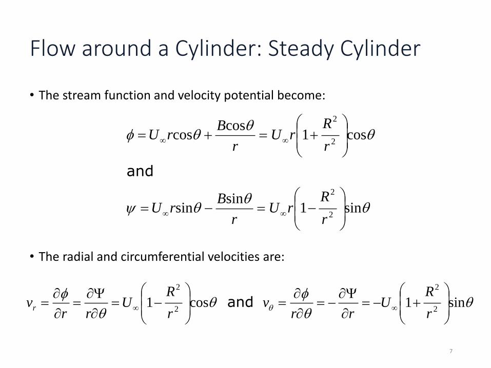
• The stream function and velocity potential become:

• The radial and circumferential velocities are:

sin1sin

sin

cos1cos

cos

2

2

2

2

r

RrU

r

BrU

r

RrU

r

BrU

and

sin1 cos1

2

2

2

2

r

RU

rrv

r

RU

rrvr and

Flow around a Cylinder: Steady Cylinder

7

Steady Cylinder

On the cylinder surface (r = R)

Normal velocity (vr) is zero, Tangential velocity (v) is non-zero slip condition.

sin2 0 Uvvr and

8

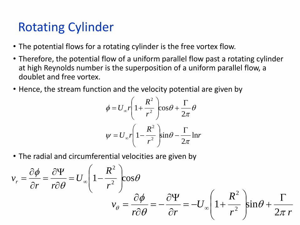
Rotating Cylinder

• The potential flows for a rotating cylinder is the free vortex flow.

• Therefore, the potential flow of a uniform parallel flow past a rotating cylinder at high Reynolds number is the superposition of a uniform parallel flow, a doublet and free vortex.

• Hence, the stream function and the velocity potential are given by

• The radial and circumferential velocities are given by

rr

RrU

r

RrU

ln2

sin1

2cos1

2

2

2

2

cos1

2

2

r

RU

rrvr

rr

RU

rrv

2sin1

2

2

9

Rotating Cylinder• The stagnation points occur at

• From

0ssr vv

0cos12

2

s

sr

RU 0

srv

0cos ss Rr :B Case OR :A Case

2

12

22

41 &

4sin

14

02

sin2 :

RURyRx

RURy

RU

RUvRr

ssss

sss

:A Case

when exits only Solution

10

Lift Force• The force per unit length of cylinder due to pressure on the cylinder surface

can be obtained by integrating the surface pressure around the cylinder.

• The tangential velocity along the cylinder surface is obtained by letting r = R,

• The surface pressure p0 as obtained from Bernoulli equation is

• where p is the pressure at far away from the cylinder (free stream)

0

02

sin2R

Ur

vRr

2

2

2sin2 2

2

0

U

pR

U

p

11

Lift Force• Hence,

• The force due to pressure in x and y directions are then obtained by

222

22

2

04

sin2

sin412

URRU

Upp

] sin cos[ 000 jisjiF dRpdRpdpFFCC

yx

URdpF

RdpFD

y

x

2

00

2

00

sin

0cos:arg

:Lift and

ji drd o sincos swhere

12

13

Stream Lines

Flow Around a Cylinder

Pressure FieldForces in the Body

http://www.diam.unige.it/~irro/cilindro_e.html

2-D Inviscid Incompressible Flow

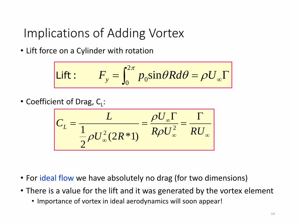
Implications of Adding Vortex• Lift force on a Cylinder with rotation

• Coefficient of Drag, CL:

• For ideal flow we have absolutely no drag (for two dimensions)

• There is a value for the lift and it was generated by the vortex element• Importance of vortex in ideal aerodynamics will soon appear!

URdpFy 2

00sin:Lift

RUUR

U

RU

LCL 2

2 )1*2(2

1

14

Is it possible?

• All this is not for nothing

• Imagine a group of sources/sinks along the x-axis such that sum of flow rates is zero• We get a closed body

• Can we select the strength of sources and sinks to fix the stagnation streamline to be the airfoil surface?• Basis of the source panel method

15

Kutta-Joukovsky Theorem

Martin Wilhelm Kutta

(1867 – 1944)

Nikolay Yegorovich Joukovsky

(1847-1921

The Kutta–Joukowsky Theorem is a fundamental theorem of

Aerodynamics. The theorem relates the Lift generated by a right

cylinder to the speed of the cylinder through the fluid, the density

of the fluid, and the Circulation.

The Circulation is defined as the line integral, around a closed

loop enclosing the cylinder or airfoil, of the component of the

velocity of the fluid tangent to the loop. The magnitude and

direction of the fluid velocity change along the path.

The force per unit length acting on a right cylinder of any

cross section whatsoever is equal to ρ∞U ∞Γ, and is

perpendicular to the direction of U ∞.

Kutta–Joukowsky Theorem:

cos: dlVldV

Circulation

2-D Inviscid Incompressible Flow

UL Kutta–Joukowsky Theorem:

LCUL2

2

1 Lift/unit area:

Kutta in 1902 and Joukowsky in 1906, independently, arrived to this result. 16

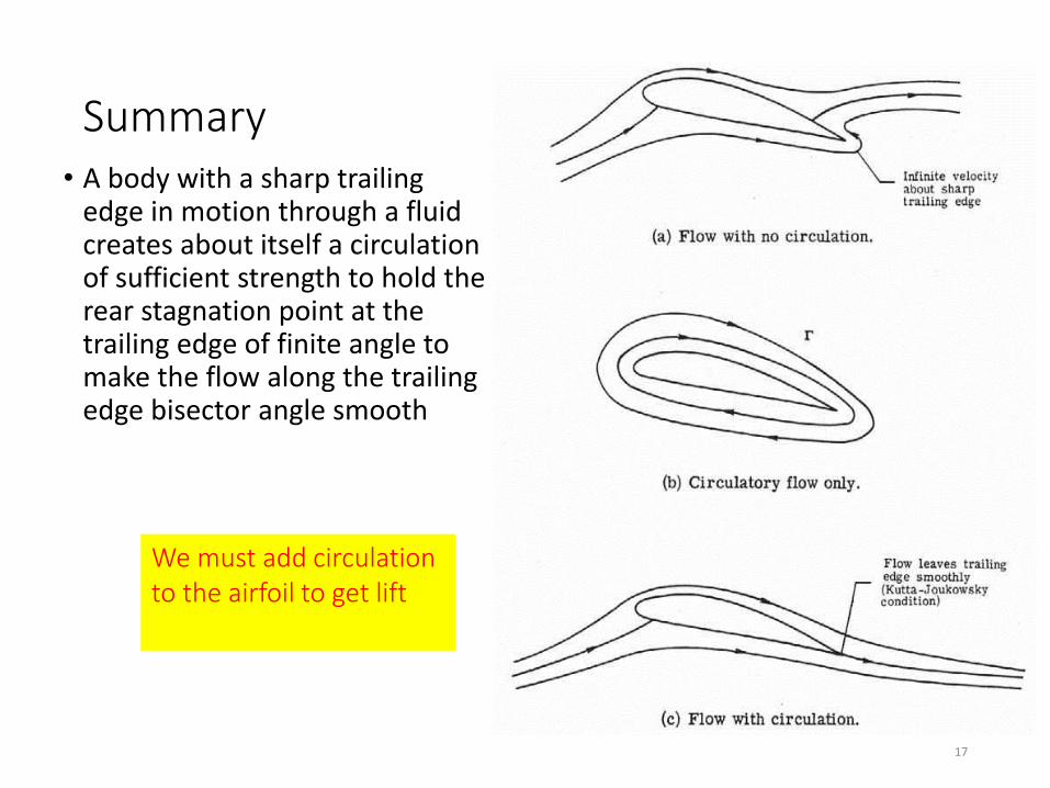
Summary• A body with a sharp trailing

edge in motion through a fluid creates about itself a circulation of sufficient strength to hold the rear stagnation point at the trailing edge of finite angle to make the flow along the trailing edge bisector angle smooth

We must add circulation to the airfoil to get lift

17

Martin Wilhelm

Kutta

(1867 – 1944)

Kutta Condition• We want to obtain an analogy between a Flow around an Airfoil

and that around a Spinning Cylinder.

For the Spinning Cylinder, when a Vortex is Superimposed with a

Doublet on an Uniform Flow, a Lifting Flow is generated.

• The Doublet and Uniform Flow don’t generate Lift.

• The generation of Lift is always associated with Circulation.

• Suppose that it is possible to use Vortices to generate Circulation, and therefore Lift, for the Flow around an Airfoil.

• Figure (a) shows the pure non-circulatory Flow around an Airfoil at an Angle of Attack. We can see the Fore SF and Aft SA Stagnation Points.

• Figure (b) shows a Flow with a Small Circulation added. The Aft Stagnation Point Remains on the Upper Surface.

• Figure (c) shows a Flow with Higher Circulation, so that the Aft Stagnation Point moves to Lower Surface. The Flow has to pass around the Trailing Edge.

• Figure (d) shows the only possible position for the Aft Stagnation Point, on the Trailing Edge.

• This is the Kutta Condition, introduced by Wilhelm Kutta in 1902,

18

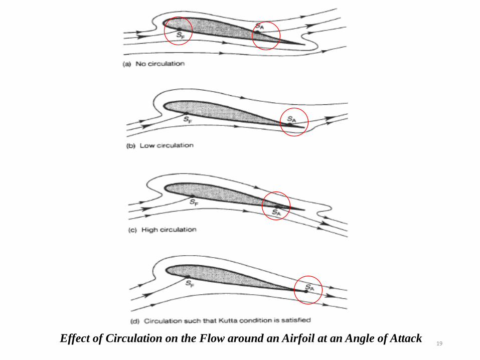
Effect of Circulation on the Flow around an Airfoil at an Angle of Attack19

The Starting Vortex

• Prandlt realized (and visualized in 1934) that there was a starting vortexhttps://www.youtube.com/watch?v=VcggiVSf5F8

• The flow over an airfoil can have a stagnation point momentarily on the upper surface

• After some time, the vortex is convected downstream to infinity.

• The value of the circulation of the starting vortex is the value of the circulation needed to create lift.

20

21

Prandtl’s Experimental Photo of Starting Vortex

22

The Starting Vortex

|airfoil|=|starting|

23

Starting (Shed) Vortex

24

25

Prandtl Lifting Line Theory

Bound Vortex

Tip Vortex

Three dimensional version of Bound Vortex Theory

A continuous line of bound vortices terminating at

the wing tips with “tip vortices” that continue

downstream to the “starting vortex”. 26

Photos of Tip Vortices

27

GENERAL THIN-AIRFOIL THEORYThe essential assumptions of thin-airfoil theory are:

(1) the lifting characteristics of an airfoil below stall are negligibly

affected by the presence of the boundary layer,

(2) the airfoil is operating at a small angle of attack, and

(3) the resultant of the pressure forces (magnitude, direction, and

line of action) is only slightly influenced by the airfoil

thickness, since the maximum mean camber is small and the

ratio of maximum thickness to chord is small.

• A velocity difference across the infinitely thin profile which represents the airfoil section is required to produce the lift-generating pressure difference.

• This results directly from the concept of circulation, which states that unless there is a local curvature to the flow there cannot be circulation and lift.

• The only way for the flow to turn is for the fluid above the airfoil to travel faster than the fluid below the airfoil.

28

GENERAL THIN-AIRFOIL THEORY

For a free vortex, (from lec. 6)

29

• A vortex sheet coincident with the mean camber line produces a velocity distribution that exhibits the required velocity jump (which is the difference in velocity between the upper and lower surfaces of the mean camber line).

• Therefore, the desired flow will be obtained by superimposing on a uniform flow a field induced by an infinite series of line vortices of infinitesimal strength which are located along the camber line.

• The total circulation is the sum of the circulations of the vortex filaments:

• where (s) is the distribution of vorticity (or vortex strength) for the line vortices. The length of an arbitrary element of the camber line is ds and positive circulation is in the clockwise direction.

• The velocity field around the sheet is the sum of the free-stream velocity and the velocity induced by all the vortex filaments that make up the vortex sheet (potential flow satisfies Laplace’s equation)

c

sds0

30

GENERAL THIN-AIRFOIL THEORY• For the vortex sheet to be a streamline of the flow, it is necessary that

the resultant velocity be tangent to the mean camber line at each point .Therefore, the sum of the components normal to the surface for these two velocities must be zero.

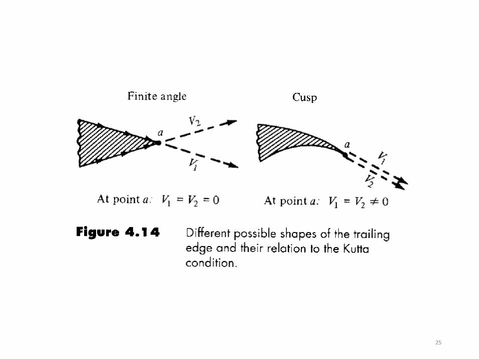
• In addition, the condition that the flows from the upper surface and the lower surface join smoothly at the trailing edge (i.e., the Kutta condition) requires that = 0 at the trailing edge.

• Ideally the circulation that forms places the rear stagnation point exactly on the sharp trailing edge. When the effects of friction are included, there is a reduction in circulation relative to the value determined for an “inviscid flow.

• Therefore, the Kutta condition places a constraint on the vorticity distribution that is consistent with the effects of the boundary layer—in other words, the Kutta condition is a viscous boundary condition based on physical observation which we will use with our inviscid theoretical development.

31

GENERAL THIN-AIRFOIL THEORY

• The portion of the vortex sheet designated ds produces a velocity (dVs) at point P which is perpendicular to the line whose length is r and which joins the element ds and the point P .

• The induced velocity component normal to the camber line at P due to the vortex element ds is:

r

dsVd ns

2

cos 3,

32

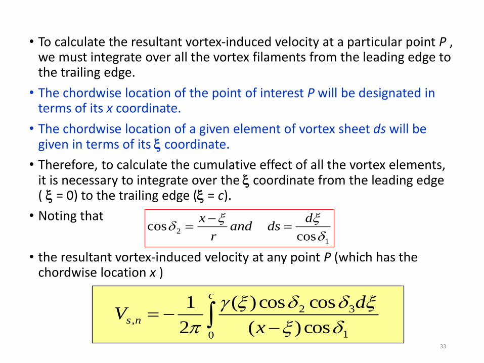
• To calculate the resultant vortex-induced velocity at a particular point P , we must integrate over all the vortex filaments from the leading edge to the trailing edge.

• The chordwise location of the point of interest P will be designated in terms of its x coordinate.

• The chordwise location of a given element of vortex sheet ds will be given in terms of its coordinate.

• Therefore, to calculate the cumulative effect of all the vortex elements, it is necessary to integrate over the coordinate from the leading edge ( = 0) to the trailing edge ( = c).

• Noting that

• the resultant vortex-induced velocity at any point P (which has the chordwise location x )

1

2cos

cos

ddsand

r

x

c

nsx

dV

0 1

32,

cos)(

coscos)(

2

1

33

34

GENERAL THIN-AIRFOIL THEORY

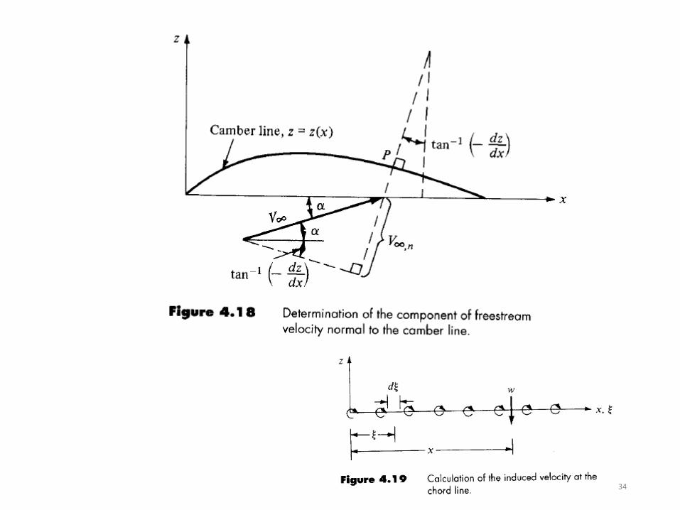
• Likewise, the component of the free-stream velocity normal to the mean camber line at P is given by:

U,n (x) = U sin( - P)

• where is the angle of attack and P is the slope of the camber line at the point of interest P :

• where z ( x ) is the function that describes the mean camber line. As a result,

• Since the sum of the velocity components normal to the surface must be zero at all points along the vortex sheet

)tansin(cos)(

coscos)(

2

1 1

0 1

32

dx

dzU

x

dc

)tansin()( 1

,dx

dzUxU n

dx

dzp

1tan

35

GENERAL THIN-AIRFOIL THEORY• The vorticity distribution () that satisfies this integral equation makes

the vortex sheet (and, therefore, the mean camber line) a streamline of the flow.

• The desired vorticity distribution must also satisfy the Kutta conditionthat (c) = 0.

• Within the assumptions of thin-airfoil theory, the angles 1, 2, 3, and are small.

• Using the approximate trigonometric relations for small angles,

• This is the fundamental equation of thin airfoil theory, which is simply the boundary condition requiring that no flow crosses the mean camber line.

)()(

2

1

0dx

dzU

x

dc

6.5

36

THIN, FLAT-PLATE AIRFOIL (SYMMETRIC AIRFOIL)

• For this case, the mean camber line is coincident with the chord line, and the geometry is just a thin flat plate.

• The approximate theoretical solution for a thin airfoil with two sharp edges represents an irrotational flow with finite velocity at the trailing edge.

• Because it does not account for the thickness distribution nor for the viscous effects, the approximate solution does not describe the chordwise variation of the flow around the actual airfoil.

• However, the theoretical values of the lift coefficient (obtained by integrating the circulation distribution along the airfoil) are in reasonable agreement with the experimental values.

• For the camber line of the symmetric airfoil, dz/dx is everywhere zero, and equation (6.5) becomes:

37

• It is convenient to introduce the coordinate transformation:

• Similarly, the x coordinate transforms to 0 using:

• The corresponding limits of integration become:

• = 0 at = 0 and = c at =

• The required vorticity distribution, (), must not only satisfy this integral equation, but must also satisfy the Kutta condition, namely that () = 0. The solution requires performing an integral of an unknown function, (), to determine a known result, U.

Ux

dc

0

)(

2

1

dc

dandc

sin2

)cos1(2

)cos1(2

0c

x

U

d

cc

dc

0 000

)cos(cos

sin)(

2

1

)cos1(2

)cos1(2

sin2

)(

2

1

6-7

38

• However, using the concept of the anti-derivative we can obtain:

• This is a valid solution, as can be seen by substituting the expression for () given by equation (6.9) into equation (6.8).

• The resulting equation,

• can be reduced to an identity using the relation:

• where n assumes only integer values. Using l’Hospital’s rule, we can show that the expression for () also satisfies the Kutta condition, since:

• which is undefined. So, taking the derivative of the numerator and denominator yields:

• which is the Kutta condition.

sin

cos12)(

U

U

dU

0 0 )cos(cos

)cos1(

0

0

0 0 sin

sin

coscos

cos

ndn

0

0

sin

cos12)(

U

0cos

sin2)(

U

6-10

6-9

39

Theoretical Lift

• The lift per unit span is therefore:

• Using the circulation distribution of equation (6.9) and the coordinate transformation of equation (6.7), the lift per unit span is

• And Cl is given by:

• where is the angle of attack in radians.

• If we take the derivative of the lift coefficient with respect to the angle of attack, we can find the lift-curve slope as C l = 2 1/rad = 0.1097 1/deg,

c

dUl0

)(

cUdcUl

2

0

2 )cos1(

2

2

1

2

1 2

2

2

cU

cU

cU

lCl

40

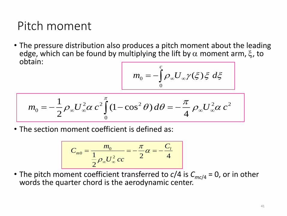
Pitch moment

• The pressure distribution also produces a pitch moment about the leading edge, which can be found by multiplying the lift by moment arm, , to obtain:

• The section moment coefficient is defined as:

• The pitch moment coefficient transferred to c/4 is Cmc/4 = 0, or in other words the quarter chord is the aerodynamic center.

c

dUm0

0 )(

22

0

222

04

)cos1(2

1cUdcUm

42

2

1 2

00

lm

C

ccU

mC

41

Center of pressure xcp

• The center of pressure xcp is the x coordinate where the resultant lift force could be placed to produce the pitch moment m0.

• Equating the moment about the leading edge to the product of the lift and the center of pressure gives us:

• Solving for xcp, we obtain:

• which is also the quarter chord of the airfoil.

• The result is independent of the angle of attack and is therefore independent of the section lift coefficient.

• The center of pressure being at c/4 implies that the distribution of pressure on the airfoil is not symmetric, but rather the pressure difference is higher near the leading edge.

• In other words, more lift is produced near the leading edge of the airfoil than near the trailing edge.

cpcxUcU 222

4

4

cxcp

42

Ex.6.1. Theoretical aerodynamic coefficients for a symmetric airfoil

• Data are presented for two different airfoil sections.

• One, the NACA 0009 airfoil, has a maximum thickness which is 9% of the chord and is located at x = 0.3c .

• The theoretical lift coefficient calculated using equation is in excellent agreement with the data for the NACA 0009 airfoil up to an angle of attack of 12.

• At higher angles of attack, the viscous effects significantly alter the flow field and hence the experimental lift coefficients.

• That is why the theoretical values would not be expected to agree with the data at high angles of attack in the stall region.

• According to thin-airfoil theory, the moment about the quarter chord is zero.

• The measured moments for the NACA 0009 are also in excellent agreement with thin-airfoil theory prior to stall.

43

NACA 0009

44

NACA 0012-64 airfoilNACA 0012-64

• The first integer (6) indicates the relative magnitude of the leading-edge radius (normal leading-edge radius is “6”; sharp leading edge is “0”).

• The second integer (4) indicates the location of the maximum thickness in tenths of chord.

• The correlation between the theoretical values and the experimental values is not as good for the NACA 0012-64 airfoil section, although the theory is very close to the data.

• The difference in the correlation between theory and data for these two airfoil sections is attributed to viscous effects since the maximum thickness of the NACA 0012-64 is greater and located farther aft.

• Therefore, the adverse pressure gradients that cause separation of the viscous boundary layer and thereby alter the flow field would be greater for the NACA 0012-64 airfoil.

• In both cases, thin-airfoil theory does a very good job of predicting the lift and moment coefficients of the airfoils.

45

NACA 0009

46

Example for Flat Plate

• Consider a thin flat plate at 5 deg. angle of attack. Calculate the: 1. lift coefficient

2. moment coefficient about the leading edge,

3. moment coefficient about the quarter chord

4. moment coefficient about the trailing edge.

47

28

For a flat plate wing section airfoil where the mean camber line equation is

(z/c) = 0 for 0 =< (x/c) =< 1

Using thin airfoil theory we can calculate the following

the zero lift angle of attack αo = 0 rad = 0o,

the pitching moment coefficient at the aerodynamic center (Cm)ac = 0,

When the angle of attack is “α=8o ”,

the lift coefficient CL = 0.8773,

the pitching moment coefficient at the leading edge (Cm)LE = −0.2193

the center of pressure (xc.p/c) = 0.25

the aerodynamic center (xac/c) = 0.25

Flat plate

48

THIN, CAMBERED AIRFOIL

• The method of determining the aerodynamic characteristics for a cambered airfoil is similar to that followed for the symmetric airfoil.

• A vorticity distribution, (), is sought which satisfies both the condition that the mean camber line is a streamline and the Kutta condition.

• Again, we will use the coordinate transformation:

• and the fundamental equation of thin-airfoil theory:

dc

dandc

sin2

)cos1(2

)()cos(cos

sin)(

2

1

0 0 dx

dzU

d

49

Vorticity Distribution

• The desired vorticity distribution, which satisfies the equation and the Kutta condition, may be represented by a series involving:

• A term of the form for the vorticity distribution for a symmetric airfoil,

• A Fourier sine series whose terms automatically satisfy the Kutta condition,

• The coefficients An of the Fourier series depend on the shape of the mean camber line.

• Putting these two requirements together gives:

• Since each term is zero when = , the Kutta condition is satisfied

)sinsin

cos1(2)(

1

0

nAAU

n

n

nAU n

n

sin21

sin

cos12 0

AU

6.20

50

• Substituting the vorticity distribution into equation (6.19) yields

• This integral equation can be used to evaluate the coefficients A0, A1, A2, …, An in terms of the angle of attack and the mean camber-line slope, which is known for a given airfoil section.

• The first integral on the left-hand side of equation (6.21) can be readily evaluated.

• To evaluate the series of integrals represented by the second term, we must use equation (6.10) and the trigonometric identity:

• Using this approach, equation (6.21) becomes:

dx

dzdnAdA

n

n

0 1 00 0

0

coscos

sinsin1

coscos

)cos1(

2

16.21

}])1cos{(})1[cos{(2

1))(sin(sin nnn

nAAdx

dz

n

n cos1

0

6.22

51

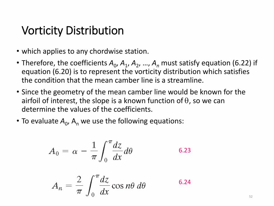
Vorticity Distribution

• which applies to any chordwise station.

• Therefore, the coefficients A0, A1, A2, …, An must satisfy equation (6.22) if equation (6.20) is to represent the vorticity distribution which satisfies the condition that the mean camber line is a streamline.

• Since the geometry of the mean camber line would be known for the airfoil of interest, the slope is a known function of , so we can determine the values of the coefficients.

• To evaluate A0, An we use the following equations:

6.23

6.24

52

Aerodynamic Coefficients for a Cambered Airfoil

• The lift and the moment coefficients for a cambered airfoil are found using the same approach as for the symmetric airfoil.

• The section lift coefficient is given by

• Notice that for any value of n other than unity. Therefore, after integration we obtain:

cU

dU

cU

lC

c

l2

0

2

2

1

)(

2

1

53

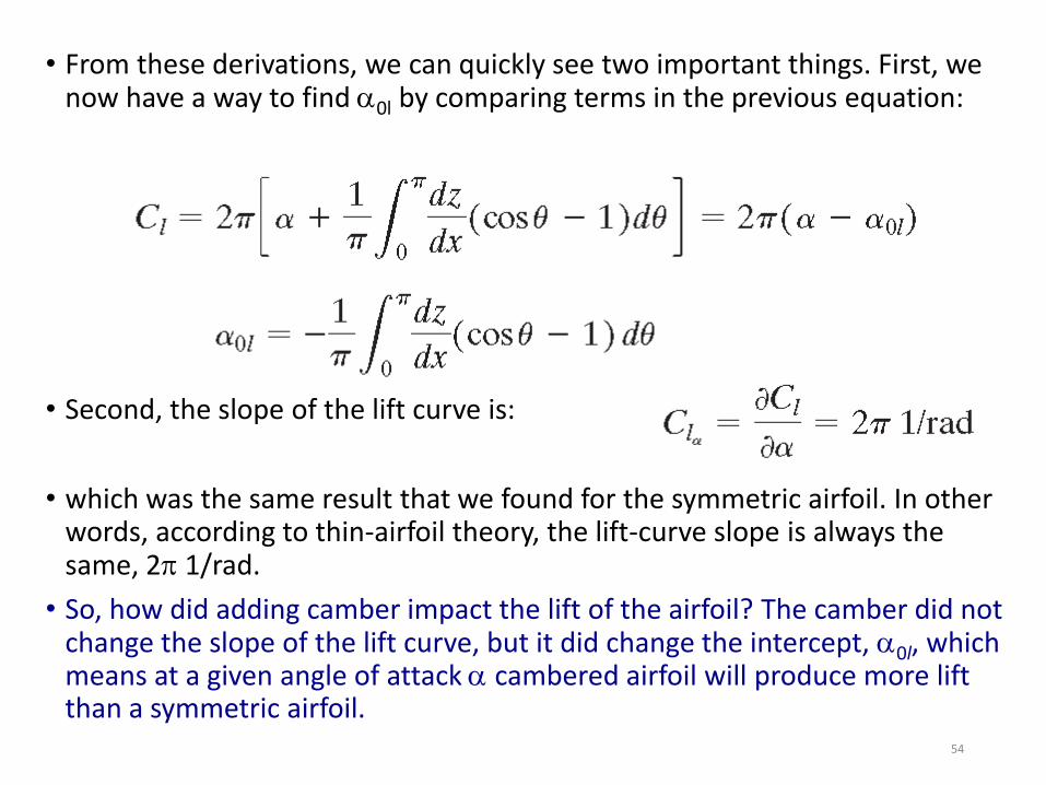
• From these derivations, we can quickly see two important things. First, we now have a way to find 0l by comparing terms in the previous equation:

• Second, the slope of the lift curve is:

• which was the same result that we found for the symmetric airfoil. In other words, according to thin-airfoil theory, the lift-curve slope is always the same, 2 1/rad.

• So, how did adding camber impact the lift of the airfoil? The camber did not change the slope of the lift curve, but it did change the intercept, 0l, which means at a given angle of attack cambered airfoil will produce more lift than a symmetric airfoil.

54

Aerodynamic Coefficients for a Cambered Airfoil

• The section moment coefficient for the pitching moment about the leading edge is given by

• Again, using the coordinate transformation and the vorticity distribution, we can integrate and obtain:

• The center of pressure relative to the leading edge is again found by dividing the moment about the leading edge (per unit span) by the lift per unit span.

• The negative sign is used since a positive lift force with a positive moment arm xcp results in a nose-down, or negative moment, as shown in the sketch of Fig. 6.7 . Therefore, the center of pressure is:

55

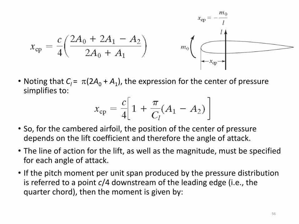
• Noting that Cl = (2A0 + A1), the expression for the center of pressure simplifies to:

• So, for the cambered airfoil, the position of the center of pressure depends on the lift coefficient and therefore the angle of attack.

• The line of action for the lift, as well as the magnitude, must be specified for each angle of attack.

• If the pitch moment per unit span produced by the pressure distribution is referred to a point c/4 downstream of the leading edge (i.e., the quarter chord), then the moment is given by:

56

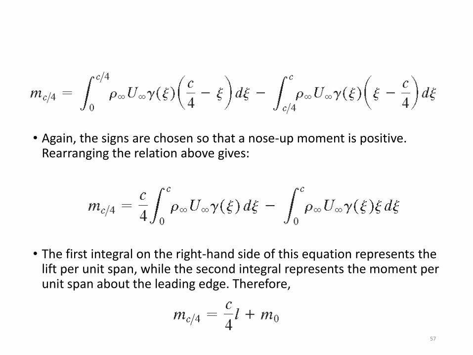
• Again, the signs are chosen so that a nose-up moment is positive. Rearranging the relation above gives:

• The first integral on the right-hand side of this equation represents the lift per unit span, while the second integral represents the moment per unit span about the leading edge. Therefore,

57

Aerodynamic Coefficients for a Cambered Airfoil

• The section moment coefficient about the quarter-chord point is given by:

• If equation (6.24) is used to define A1 and A2, then Cmac becomes:

58

EX.6.2: Theoretical aerodynamic coefficients for a cambered airfoil

• The airfoil section selected for use in this sample problem is the NACA 2412 airfoil.

• The first digit defines the maximum camber in percent of chord, the second digit defines the location of the maximum camber in tenths of chord, and the last two digits represent the thickness ratio (i.e., the maximum thickness in percent of chord).

• The equation for the mean camber line is defined in terms of the maximum camber and its location, which for this airfoil is 0.4 c .

• Forward of the maximum camber position (0 x/c 0.4), the equation of the mean camber line is

and aft of the maximum camber position

• (0.4 x/c 1.0),

59

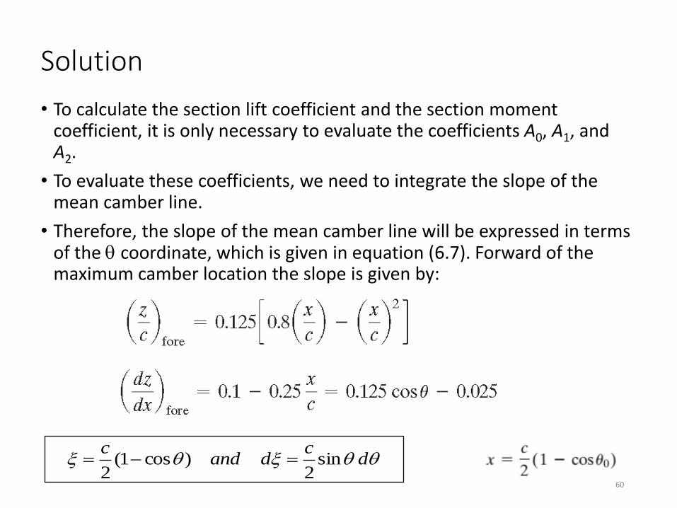
Solution

• To calculate the section lift coefficient and the section moment coefficient, it is only necessary to evaluate the coefficients A0, A1, and A2.

• To evaluate these coefficients, we need to integrate the slope of the mean camber line.

• Therefore, the slope of the mean camber line will be expressed in terms of the coordinate, which is given in equation (6.7). Forward of the maximum camber location the slope is given by:

dc

dandc

sin2

)cos1(2

60

• and aft of the maximum camber position (0.4 x/c 1.0),

• Since the maximum camber location serves as a limit for the integrals, it is necessary to convert the x coordinate, which is 0.4 c, to the corresponding coordinate.

• To do this, we use the transformation given by equation

61

• The resulting location of the maximum camber is = 78.463 = 1.3694 rad.

• Referring to equations (6.23) and (6.24), the necessary coefficients are:

62

cambered airfoil

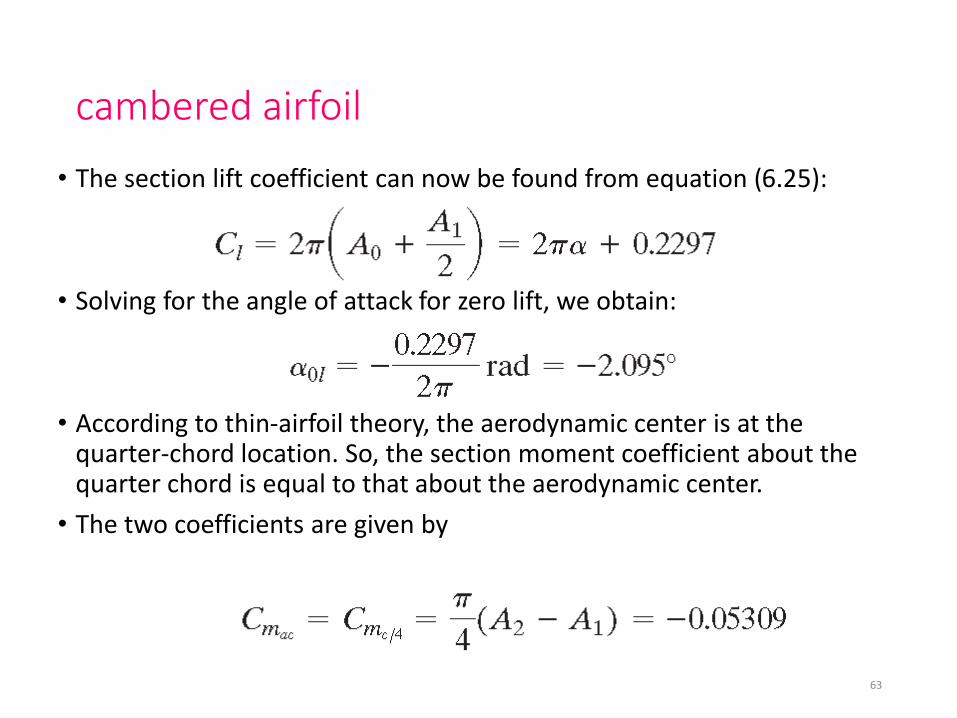
• The section lift coefficient can now be found from equation (6.25):

• Solving for the angle of attack for zero lift, we obtain:

• According to thin-airfoil theory, the aerodynamic center is at the quarter-chord location. So, the section moment coefficient about the quarter chord is equal to that about the aerodynamic center.

• The two coefficients are given by

63

Comparison with exp. data• Since the theoretical coefficients do not depend on the airfoil section

thickness, they will be compared with data for a NACA 2418 airfoil as well as for a NACA 2412 airfoil.

• For both airfoil sections, the maximum camber is 2% of the chord length and is located at x = 0.4c.

• The maximum thickness is 12% of chord for the NACA 2412 airfoil section and is 18% of the chord for the NACA2418 airfoil section. While an 18% thick airfoil is not considered “thin,” it will be informative to see how well thin-airfoil theory does at predicting the aerodynamics of this airfoil.

• The correlation between the theoretical and the experimental values of lift coefficient is satisfactory for both airfoils until the angle of attack becomes so large that viscous phenomena significantly affect the flow field.

• The theoretical value for the zero lift angle of attack agrees very well with the measured values for the two airfoils.

64

65

cambered airfoil

• The theoretical value of C l is 2 per radian.

• Based on the measured lift coefficients for angles of attack for 0 to 10, the experimental value of C l, is approximately 6.0 per radian for the NACA 2412 airfoil and approximately 5.9 per radian for the NACA 2418 airfoil, which are 4.5% and 6.1% below 2, respectively.

• The experimental values of the moment coefficient referred to the aerodynamic center (approximately -0.045 for the NACA 2412 airfoil and -0.050 for the NACA2418 airfoil) compare favorably with the theoretical value of -0.053.

66

Detailed Solution• GOAL: Find values of cl, L=0, and cm,c/4 for a NACA 2412 Airfoil

• Maximum thickness 12 % of chord

• Maximum chamber of 2% of chord located 40% downstream of the leading edge of the chord line

• Check Out: http://www.pagendarm.de/trapp/programming/java/profiles/

Root Airfoil: NACA 2412

Tip Airfoil: NACA 0012

NACA 2412

67

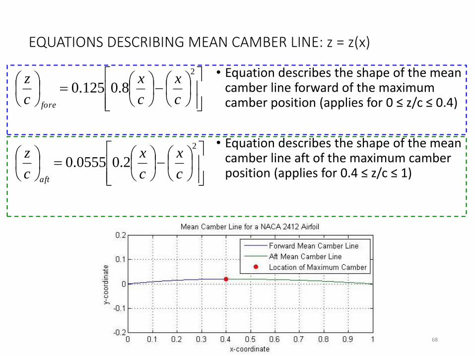
EQUATIONS DESCRIBING MEAN CAMBER LINE: z = z(x)

• Equation describes the shape of the mean camber line forward of the maximum camber position (applies for 0 ≤ z/c ≤ 0.4)

• Equation describes the shape of the mean camber line aft of the maximum camber position (applies for 0.4 ≤ z/c ≤ 1)

2

2

2.00555.0

8.0125.0

c

x

c

x

c

z

c

x

c

x

c

z

aft

fore

68

EXPRESSIONS FOR MEAN CAMBER LINE SLOPE: dz/dx

c

x

dx

dz

c

x

dx

dz

c

x

c

x

c

z

fore

fore

fore

25.01.0

28.0125.0

8.0125.0

2

c

x

dx

dz

c

x

dx

dz

c

x

c

x

c

z

aft

aft

aft

111.00444.0

28.00555.0

2.00555.0

2

69

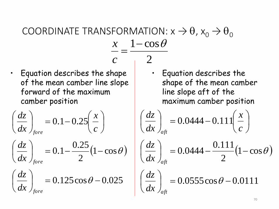
COORDINATE TRANSFORMATION: x → , x0 → 0

025.0cos125.0

cos12

25.01.0

25.01.0

fore

fore

fore

dx

dz

dx

dz

c

x

dx

dz

0111.0cos0555.0

cos12

111.00444.0

111.00444.0

aft

aft

aft

dx

dz

dx

dz

c

x

dx

dz

2

cos1

c

x

• Equation describes the shape of the mean camber line slope forward of the maximum camber position

• Equation describes the shape of the mean camber line slope aft of the maximum camber position

70

EXAMINE LIMITS OF INTEGRATION

• Coefficients A0, A1, and A2 are evaluated across the entire airfoil• Evaluated from the leading edge to the trailing edge

• Evaluated from leading edge (=0) to the trailing edge (=)

• 2 equations the describe the fore and aft portions of the mean camber line• Fore equation integrated from leading edge to location of maximum camber

• Aft equation integrated from location of maximum camber to trailing edge

• The location of maximum camber is (x/c)=0.4

• What is the location of maximum camber in terms of ?

rad 3694.1

463.78

2.0cos

4.02

cos1

cambermax

cambermax

cambermax

cambermax

c

x

71

EXAMPLE: NACA 2412 CAMBERED AIRFOIL

• Thin airfoil theory lift slope:

dcl/d = 2 rad-1 = 0.11 deg-1

• What is L=0?

• From data L=0 ~ -2º

• From theory L=0 = -2.07º

• What is cm,c/4?

• From data cm,c/4 ~ -0.045

• From theory cm,c/4 = -0.054

dcl/d = 2

72

Bounday layer Effect• Henderson (1978) notes, “Rarely will the boundary layers be thin

enough that potential flow analysis of the bare geometry will be sufficiently accurate.”

• By including the effect of the boundary layer but not the separated wake in the computational flow model, the agreement between the theoretical lift coefficients and the wind-tunnel values is good at low angles of attack, as shown in Fig. b.

• When the angle of attack is increased and separation becomes important, the predicted and the measured lift coefficients again begin to diverge.

• Separation effects must be modeled in order to predict the maximum lift coefficient.

• As shown in Fig. c, when we account for the boundary layer and the separated wake, there is good agreement between theoretical values and experimental values through Clmax.

73

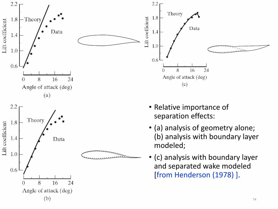
• Relative importance of separation effects:

• (a) analysis of geometry alone; (b) analysis with boundary layer modeled;

• (c) analysis with boundary layer and separated wake modeled [from Henderson (1978) ].

74

Using thin airfoil theory we can calculate the following

the zero lift angle of attack αo = − 0.0259 rad = −1.483o,

the pitching moment coefficient at the aerodynamic center (Cm)ac = −0.0244,

When the angle of attack is “α=10o ”,

the lift coefficient CL = 1.26,

the pitching moment coefficient at the leading edge (Cm)LE = −0.339

the pitching moment coefficient at the half chord point (Cm)C/2= 0.29

the center of pressure (xc.p/c) = 0.27

the aerodynamic center (xac/c) = 0.25

The NACA 25012 wing section airfoil has a mean camber line given by

NACA 25012

(z/c) = 0.5383 (x/c)3 - 0.6315 (x/c)2 + 0.2147 (x/c) for 0 =< (x/c) =< 0.391

(z/c) = 0.0322 (1 - x/c ) for 0.391 =< (x/c) =< 1

75

Example for Cambered Airfoil

• Consider an NACA 23012 airfoil. The mean camber line for this airfoil is given by

• Calculate:1. the angle of attack at zero lift,

2. the lift coefficient when = 4◦,

3. the moment coefficient about the quarter chord,

4. the location of the center of pressure in terms of xcp/c, when = 4◦.

3 2z x x x x

2.6595 0.6075 0.1147 , for 0 0.2025c c c c c

z x x2.6595 1 , for 0.2025 1.0

c c c

76

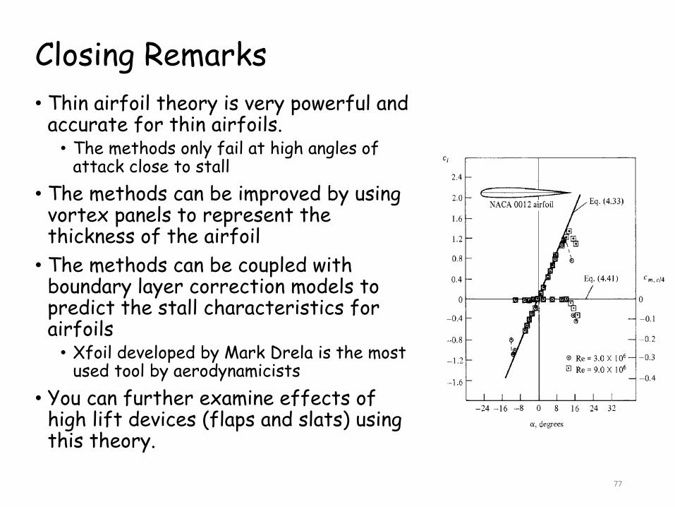
Closing Remarks

• Thin airfoil theory is very powerful and accurate for thin airfoils.• The methods only fail at high angles of

attack close to stall

• The methods can be improved by using vortex panels to represent the thickness of the airfoil

• The methods can be coupled with boundary layer correction models to predict the stall characteristics for airfoils• Xfoil developed by Mark Drela is the most

used tool by aerodynamicists

• You can further examine effects of high lift devices (flaps and slats) using this theory.

77

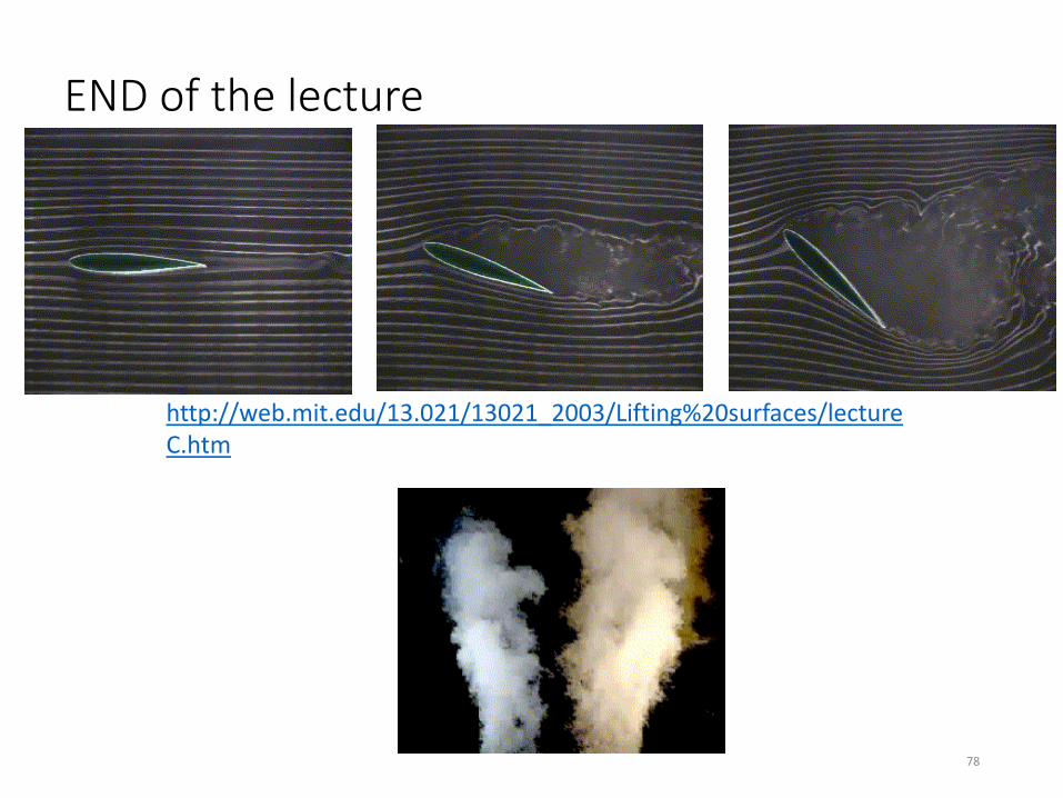
END of the lecture

http://web.mit.edu/13.021/13021_2003/Lifting%20surfaces/lectureC.htm

78