Lecture 8: Generalized large-scale structuretuvalu.santafe.edu/~aaronc/courses/5352/csci5352_2017_L8.pdf · Aaron Clauset @aaronclauset Assistant Professor of Computer Science University

100150

200250

300

Aaron Clauset @aaronclausetAssistant Professor of Computer ScienceUniversity of Colorado BoulderExternal Faculty, Santa Fe Institute

Lecture 8:Generalized large-scale structure

© 2017 Aaron Clauset

hierarchical communities

most communities are not random graphs

• groups within groups / groups of groups• finding communities at one "level" of a hierarchy

can obscure structure above or below that level

plant→

→

herbivore

→

parasite


modules


nestedmodules


can we automatically extract such hierarchies?

?

step 3: hierarchystep 1: network data


hierarchical random graph model


Clauset, Moore, Newman, Nature 453, 98-101 (2008)Clauset, Moore, Newman, ICML (2006)

D


assortative modules

D, {pr}

probability pr


“inhomogeneous” random graph

model

instance

Pr(i, j connected) = pr

i

j

i j

= p(lowest common ancestor of i,j)


Er

Rr

Lr = number nodes in left subtree

= number nodes in right subtree

= number edges with as lowest common ancestor

Lr Rr

Er

→

pr

r

Pr(A | D, {pr}) =Y

r

pErr (1� pr)

LrRr�Er}hierarchical random graph model


1

1

1/3

1

1/4

L = 0.0016

L =

!

"

1

3

#1 "

2

3

#2$

·

!

"

1

4

#2 "

3

4

#6$

L(D, {pr}) =!

r

pEr

r (1 − pr)LrRr−Er

1

1 1

1

1/9 L =

!

"

1

9

#1 "

8

9

#8$

L(D, {pr}) =!

r

pEr

r (1 − pr)LrRr−Er

L = 0.0433


generalizing from a single example

• given graph , estimate model parameters• sample new graphs from posterior distribution

checking the models

compare resampled graphs with original datacheck

1. degree distribution2. clustering coefficient3. geodesic path lengths


A D, {pr}Pr(G | D, {pr})

!"#$%$&'()')*+,$-


!"#$%$&'()')*+,$-

100 10110−3

10−2

10−1

100a

Degree, k

Frac

tion

of v

ertic

es w

ith d

egre

e k

resampled→

original→


degree distribution

!"#$%$&'()')*+,$-

resampled→

original→

0 0.05 0.1 0.15 0.2 0.25 0.30

0.05

0.1

0.15

0.2

0.25

Frac

tion

of g

raph

s w

ith c

lust

erin

g co

effic

ient

c

Clustering coefficient, c

resampled→

original→


density of triangles

2 4 6 8 1010−3

10−2

10−1

100b

Distance, d

Frac

tion

of v

erte

x−pa

irs a

t dis

tanc

e d

resampled→

original→

!"#$%$&'()')*+,$-


geodesic distances

inspecting the dendrograms


0

1

2

3

4

5

6

78

9

10

11

1213

14

15

16

17

18

19

20

21

22

23

24

25

26

27

28

29

30

31

32

33

34

35

36

37

38

3940

41

42

43

44

45

46

47

48

49

50

51

52

53

54

55

56

57

58

59

60

61

62

63

64

65

66

67

68

69

70

71

72

73

74

75

76

77

78

79

80

81

82

83

84

85

86

87

88

89

90

91

92

93

94

95 96

97

98

99

101

102

103

104

105

106

107

108

109 110

111

112

113

114

100

1

2

3

4

5

6

7

8

9

10

11

12

13

14

15

16

17

18

19

20

21

22

23

24

25 26

27

28

29

30

31

32

33

34

Zachary’s Karate ClubNCAA Schedule 2000

8 14

3

13

4

20

22

18

2

12

5

6

7

11

17 1 9

31

2315

19

21

32

29

28

24

27

30

16

33

10

34

26

25

MAP


1

2

3

4

5

6

7

8

9

10

11

12

13

14

15

16

17

18

19

20

21

22

23

24

25 26

27

28

29

30

31

32

33

34

Bri

gh

am

Yo

un

g (

0)

New

Mexic

o (

4)

San

Die

go

Sta

t (9

)W

yo

min

g (

16)

Uta

h (

23)

NV

LasV

eg

as (

104)

Air

Fo

rce (

93)

Co

lora

do

Sta

t (4

1)

NM

Sta

te (69)

Ark

ansasS

tat (2

4)

Nort

hTex

as (11

)

Bois

eSta

te (28

)

Idah

o (50

)

Uta

hSta

te (9

0)

Ore

gonSta

te (1

08)

Ariz

onaSta

te (8

)

Arizona (2

2)

Californ

ia (1

11)

WashSta

te (7

8)

UCLA (21)

Oregon (68)

Stanford (77)

SouthernCal (7)

Washington (51)

Hawaii (114)

Nevada (67)

TexasElPaso (83)

FresnoState (46)

TXChristian (110)Tulsa (88)SanJoseState (73)Rice (49)SouthernMeth (53)

FloridaState (1)WakeForest (105)

Maryland (109)

Clemson (103)

NCState (25)

Duke (45)

Virginia (33)

GeorgiaTech (37)

NoCarolina (89)

WesternM

ich (14)

CentralM

ich (38)

NorthernIll (12)

BallS

tate (26)

Toled

o (85)

Eastern

Mich

(43)

Akro

n (1

8)

Buffa

lo (3

4)

Oh

io (7

1)

Ken

t (54)

Mars

hall (9

9)

Bo

wlin

gG

reen

(31)

Mia

miO

hio

(61)

Co

nn

ectic

ut (4

2)

Mis

sS

tate

(65)

Lo

uis

ian

Sta

t (96)

(62)V

an

derb

ilt

(95)G

eo

rgia

(17)A

ub

urn

(87)M

issis

sip

pi

(70)S

oC

aro

lin

a

(76)T

en

nessee

(27)F

lori

da

(56)K

en

tucky

(113)A

rkansas

(20)A

labam

a

(101

)Mia

miF

lori

da

(19)

Virgin

iaTec

h

(30)

Wes

tVirgi

nia

(35)

Syr

acus

e

(55)

Pittsb

urgh

(80)N

avy

(29)B

ostonColl

(79)T

emple

(94)Rutg

ers

(39)Purdue

(32)Michigan(2)Iowa

(47)OhioState

(13)Northwestern(106)Indiana(60)Minnesota(100)MichiganStat(64)Illinois

(6)PennState(15)Wisconsin

(74)Nebraska

(52)Kansas

(3)KansasState

(10)Baylor

(98)Texas

(107)OKState

(81)TexasA&M

(72)IowaState

(40)Colorado

(102)Missouri

(84)Oklahoma

(5)TexasTech

(82)NotreD

ame

(57)Louisville

(66)Mem

phis

(75)South

ernM

iss

(91)Arm

y

(86)Tulan

e

(48)H

ousto

n

(112)A

LB

irmin

gham

(92)C

incin

nati

(44)E

astC

aro

lina

(97)L

ou

isia

naL

af

(63)M

idT

NS

tate

(36)C

en

tFlo

rida

(59)L

ou

isia

nM

on

r(5

8)L

ou

isia

nT

ech


0

1

2

3

4

5

6

78

9

10

11

1213

14

15

16

17

18

19

20

21

22

23

24

25

26

27

28

29

30

31

32

33

34

35

36

37

38

3940

41

42

43

44

45

46

47

48

49

50

51

52

53

54

55

56

57

58

59

60

61

62

63

64

65

66

67

68

69

70

71

72

73

74

75

76

77

78

79

80

81

82

83

84

85

86

87

88

89

90

91

92

93

94

95 96

97

98

99

101

102

103

104

105

106

107

108

109 110

111

112

113

114

100

MAP

link prediction in networks

• many networks are sampled• social nets, foodwebs, protein interactions, etc.• generative models provide estimate of

for either (missing links) or (spurious links)• like cross-validation: hold out some adjacencies,

measure accuracy of algorithm on these

now many approaches to link prediction:• Liben-Nowell & Kleinberg (2003)• Goldberg & Roth (2003)• Szilágyi et al. (2005)• Guimera & Sales-Pardo (2009)• and many others


Pr(Aij | ✓)Aij = 0 Aij = 1

{Aij}

http://www.cs.carleton.edu/faculty/dlibenno/papers/link-prediction/link.pdf

http://www.ncbi.nlm.nih.gov/pubmed/12676999

http://iopscience.iop.org/article/10.1088/1478-3975/2/2/S01/meta

http://www.pnas.org/content/106/52/22073

!"#$%$&'()')*+,$-

0 0.2 0.4 0.6 0.8 10.4

0.5

0.6

0.7

0.8

0.9

1

Area

und

er R

OC

cur

ve

Fraction of edges observed, k/m

Grassland species network

Pure chanceCommon neighborsJaccard coeff.Degree productShortest pathsHierarchical structure

simple predictors

hierarchy

pure chance

AUC


0 0.2 0.4 0.6 0.8 10.4

0.5

0.6

0.7

0.8

0.9

1

AUC

Fraction of edges observed

Terrorist association networka

Pure chanceCommon neighborsJaccard coefficientDegree productShortest pathsHierarchical structure

0 0.2 0.4 0.6 0.8 10.4

0.5

0.6

0.7

0.8

0.9

1

AUC

Fraction of edges observed

T. pallidum metabolic networkb

Pure chanceCommon neighborsJaccard coefficientDegree productShortest pathsHierarchical structure


other approaches


other approaches

edge counts among blocks are another networkfit another SBM to these, repeat


Hierarchical Block Structures and High-Resolution Model Selection in Large Networks

Tiago P. Peixoto*

Institut für Theoretische Physik, Universität Bremen, Hochschulring 18, D-28359 Bremen, Germany(Received 5 November 2013; published 24 March 2014)

Discovering and characterizing the large-scale topological features in empirical networks are crucialsteps in understanding how complex systems function. However, most existing methods used to obtain themodular structure of networks suffer from serious problems, such as being oblivious to the statisticalevidence supporting the discovered patterns, which results in the inability to separate actual structure fromnoise. In addition to this, one also observes a resolution limit on the size of communities, where smaller butwell-defined clusters are not detectable when the network becomes large. This phenomenon occurs for thevery popular approach of modularity optimization, which lacks built-in statistical validation, but also formore principled methods based on statistical inference and model selection, which do incorporate statisticalvalidation in a formally correct way. Here, we construct a nested generative model that, through a completedescription of the entire network hierarchy at multiple scales, is capable of avoiding this limitation andenables the detection of modular structure at levels far beyond those possible with current approaches. Evenwith this increased resolution, the method is based on the principle of parsimony, and is capable ofseparating signal from noise, and thus will not lead to the identification of spurious modules even on sparsenetworks. Furthermore, it fully generalizes other approaches in that it is not restricted to purely assortativemixing patterns, directed or undirected graphs, and ad hoc hierarchical structures such as binary trees.Despite its general character, the approach is tractable and can be combined with advanced techniques ofcommunity detection to yield an efficient algorithm that scales well for very large networks.

DOI: 10.1103/PhysRevX.4.011047 Subject Areas: Complex Systems, InterdisciplinaryPhysics, Statistical Physics

I. INTRODUCTION

The detection of communities and other large-scalestructures in networks has become perhaps one of thelargest undertakings in network science [1,2]. It is moti-vated by the desire to be able to characterize the mostsalient features in large biological [3–5], technological[6,7], and social systems [3,8,9], such that their buildingblocks become evident, potentially giving valuable insightinto the central aspects governing their function andevolution. At its simplest level, the problem seems straight-forward: Modules are groups of nodes in the network thathave a similar connectivity pattern, often assumed to beassortative, i.e., connected mostly among themselves andless so with the rest of the network. However, whenattempting to formalize this notion and develop methodsto detect such structures, the combined effort of manyresearchers in recent years has spawned a great variety ofcompeting approaches to the problem, with no clear,universally accepted outcome [2].

The method that has perhaps gathered the most wide-spread use is called modularity optimization [10] andconsists in maximizing a quality function that favorspartitions of nodes for which the fraction of internal edgesinside each cluster is larger than expected given a nullmodel, taken to be a random graph. This method isrelatively easy to use and comprehend, works well inmany accessible examples, and is capable of being appliedin very large systems via efficient heuristics [11,12].However it also suffers from serious drawbacks. In par-ticular, despite measuring a deviation from a null model, itdoes not take into account the statistical evidence asso-ciated with this deviation, and as a result, it is incapable ofseparating actual structure from those arising simply ofstatistical fluctuations of the null model, and it even findshigh-scoring partitions in fully random graphs [13]. Thisproblem is not specific to modularity and is a characteristicshared by the vast majority of methods proposed forsolving the same task [2]. In addition to the lack ofstatistical validation, modularity maximization fails todetect clusters with size below a given threshold [14,15],which increases with the size of the system as ∼

ffiffiffiffiE

p, where

E is the number of edges in the entire network. Thislimitation is independent of how salient these relativelysmaller structures are, and makes this potentially very im-portant information completely inaccessible. Furthermore,

*[email protected]‑bremen.de

Published by the American Physical Society under the terms ofthe Creative Commons Attribution 3.0 License. Further distri-bution of this work must maintain attribution to the author(s) andthe published article’s title, journal citation, and DOI.

PHYSICAL REVIEW X 4, 011047 (2014)

2160-3308=14=4(1)=011047(18) 011047-1 Published by the American Physical Society

l =0

l =1

l =2

l =3

Nested

model

Observed

network

N nodes

E edges

B0 nodes

E edges

B1 nodes

E edges

B2 nodes

E edges

ers

Peixoto, Phys. Rev. X 4, 011047 (2014)


Peixoto, Phys. Rev. X 4, 011047 (2014)

other approaches (hierarchical SBM)

political blogs (2004) network

limits of statistical inference


community structure in networks

• dozens of algorithms for finding it• generative models among the most powerful• how methods fail is as important as how they succeed

• even if communities exist in a network, they may not be detectable


planted partition problem

• synthetic data with known communities• 2 groups, equal sized• mean degree• parameterized strength of communities

cout

n

cinn

cinn

cout

n

c

✏ = cout

/cin

Decelle, Krzakala, Moore, & Zdeborová, Phys. Rev. Lett. 107, 065701 (2011)



• synthetic data with known communities• 2 groups, equal sized• mean degree c

✏ = cout

/cin


13

obeying detailed balance with respect to the Hamiltonian (8), starting with a random initial group assignment {qi}.We see that Q = 0 for cout/cin > ϵc. In other words, in this region both BP and MCMC converge to the factorizedstate, where the marginals contain no information about the original assignment. For cout/cin < ϵc, however, theoverlap is positive and the factorized fixed point is not the one to which BP or MCMC converge.

In particular the right-hand side of Fig. 1 shows the case of q = 4 groups with average degree c = 16, correspondingto the benchmark of Newman and Girvan [9]. We show the large N results and also the overlap computed withMCMC for size N = 128 which is the commonly used size for this benchmark. Again, up to symmetry breaking,marginalization achieves the best possible overlap that can be inferred from the graph by any algorithm. Therefore,when algorithms are tested for performance, their results should be compared to Fig. 1 instead of to the common butwrong expectation that the four groups are detectable for any ϵ < 1.

0

0.1

0.2

0.3

0.4

0.5

0.6

0.7

0.8

0.9

1

0 0.1 0.2 0.3 0.4 0.5 0.6 0.7 0.8 0.9 1

over

lap

!= cout/cin

undetectable

q=2, c=3

N=500k, BPN=70k, MCMC

0

0.2

0.4

0.6

0.8

1

0 0.2 0.4 0.6 0.8 1

over

lap

!= cout/cin

undetectable

q=4, c=16

N=100k, BPN=70k, MCN=128, MC

N=128, full BP

FIG. 1: (color online): The overlap (5) between the original assignment and its best estimate given the structure of the graph,computed by the marginalization (13). Graphs were generated using N nodes, q groups of the same size, average degree c, anddifferent ratios ϵ = cout/cin. Thus ϵ = 1 gives an Erdos-Renyi random graph, and ϵ = 0 gives completely separated groups.Results from belief propagation (26) for large graphs (red line) are compared to Gibbs sampling, i.e., Monte Carlo Markovchain (MCMC) simulations (data points). The agreement is good, with differences in the low-overlap regime that we attributeto finite size fluctuations. On the right we also compare to results from the full BP (22) and MCMC for smaller graphs withN = 128, averaged over 400 samples. The finite size effects are not very strong in this case, and BP is reasonably close to theexact (MCMC) result even on small graphs that contain many short loops. For N → ∞ and ϵ > ϵc = (c−

√c)/[c+

√c(q−1)] it

is impossible to find an assignment correlated with the original one based purely on the structure of the graph. For two groupsand average degree c = 3 this means that the density of connections must be ϵ−1

c (q = 2, c = 3) = 3.73 greater within groupsthan between groups to obtain a positive overlap. For Newman and Girvan’s benchmark networks with four groups (right),this ratio must exceed 2.33.

Let us now investigate the stability of the factorized fixed point under random perturbations to the messages whenwe iterate the BP equations. In the sparse case where cab = O(1), graphs generated by the block model are locallytreelike in the sense that almost all nodes have a neighborhood which is a tree up to distance O(log N), where theconstant hidden in the O depends on the matrix cab. Equivalently, for almost all nodes i, the shortest loop that ibelongs to has length O(log N). Consider such a tree with d levels, in the limit d → ∞. Assume that on the leavesthe factorized fixed point is perturbed as

ψkt = nt + ϵk

t , (39)

and let us investigate the influence of this perturbation on the message on the root of the tree, which we denote k0.There are, on average, cd leaves in the tree where c is the average degree. The influence of each leaf is independent,so let us first investigate the influence of the perturbation of a single leaf kd, which is connected to k0 by a pathkd, kd−1, . . . , k1, k0. We define a kind of transfer matrix

T ai ≡

∂ψkia

∂ψki+1

b

!

!

!

ψt=nt

=

"

ψkia cab

#

r carψki+1r

− ψkia

$

s

ψkis csb

#

r carψki+1r

%

!

!

!

ψt=nt

= na

&cab

c− 1

'

. (40)

where this expression was derived from (26) to leading order in N . The perturbation ϵk0

t0 on the root due to the

strong communities

random graph

easyto detect

hardto detect

over

lap

(acc

urac

y)



• synthetic data with known communities• 2 groups, equal sized• mean degree c

✏ = cout

/cin


13

obeying detailed balance with respect to the Hamiltonian (8), starting with a random initial group assignment {qi}.We see that Q = 0 for cout/cin > ϵc. In other words, in this region both BP and MCMC converge to the factorizedstate, where the marginals contain no information about the original assignment. For cout/cin < ϵc, however, theoverlap is positive and the factorized fixed point is not the one to which BP or MCMC converge.

In particular the right-hand side of Fig. 1 shows the case of q = 4 groups with average degree c = 16, correspondingto the benchmark of Newman and Girvan [9]. We show the large N results and also the overlap computed withMCMC for size N = 128 which is the commonly used size for this benchmark. Again, up to symmetry breaking,marginalization achieves the best possible overlap that can be inferred from the graph by any algorithm. Therefore,when algorithms are tested for performance, their results should be compared to Fig. 1 instead of to the common butwrong expectation that the four groups are detectable for any ϵ < 1.

0

0.1

0.2

0.3

0.4

0.5

0.6

0.7

0.8

0.9

1

0 0.1 0.2 0.3 0.4 0.5 0.6 0.7 0.8 0.9 1

over

lap

!= cout/cin

undetectable

q=2, c=3

N=500k, BPN=70k, MCMC

0

0.2

0.4

0.6

0.8

1

0 0.2 0.4 0.6 0.8 1

over

lap

!= cout/cin

undetectable

q=4, c=16

N=100k, BPN=70k, MCN=128, MC

N=128, full BP

FIG. 1: (color online): The overlap (5) between the original assignment and its best estimate given the structure of the graph,computed by the marginalization (13). Graphs were generated using N nodes, q groups of the same size, average degree c, anddifferent ratios ϵ = cout/cin. Thus ϵ = 1 gives an Erdos-Renyi random graph, and ϵ = 0 gives completely separated groups.Results from belief propagation (26) for large graphs (red line) are compared to Gibbs sampling, i.e., Monte Carlo Markovchain (MCMC) simulations (data points). The agreement is good, with differences in the low-overlap regime that we attributeto finite size fluctuations. On the right we also compare to results from the full BP (22) and MCMC for smaller graphs withN = 128, averaged over 400 samples. The finite size effects are not very strong in this case, and BP is reasonably close to theexact (MCMC) result even on small graphs that contain many short loops. For N → ∞ and ϵ > ϵc = (c−

√c)/[c+

√c(q−1)] it

is impossible to find an assignment correlated with the original one based purely on the structure of the graph. For two groupsand average degree c = 3 this means that the density of connections must be ϵ−1

c (q = 2, c = 3) = 3.73 greater within groupsthan between groups to obtain a positive overlap. For Newman and Girvan’s benchmark networks with four groups (right),this ratio must exceed 2.33.

Let us now investigate the stability of the factorized fixed point under random perturbations to the messages whenwe iterate the BP equations. In the sparse case where cab = O(1), graphs generated by the block model are locallytreelike in the sense that almost all nodes have a neighborhood which is a tree up to distance O(log N), where theconstant hidden in the O depends on the matrix cab. Equivalently, for almost all nodes i, the shortest loop that ibelongs to has length O(log N). Consider such a tree with d levels, in the limit d → ∞. Assume that on the leavesthe factorized fixed point is perturbed as

ψkt = nt + ϵk

t , (39)

and let us investigate the influence of this perturbation on the message on the root of the tree, which we denote k0.There are, on average, cd leaves in the tree where c is the average degree. The influence of each leaf is independent,so let us first investigate the influence of the perturbation of a single leaf kd, which is connected to k0 by a pathkd, kd−1, . . . , k1, k0. We define a kind of transfer matrix

T ai ≡

∂ψkia

∂ψki+1

b

!

!

!

ψt=nt

=

"

ψkia cab

#

r carψki+1r

− ψkia

$

s

ψkis csb

#

r carψki+1r

%

!

!

!

ψt=nt

= na

&cab

c− 1

'

. (40)

where this expression was derived from (26) to leading order in N . The perturbation ϵk0

t0 on the root due to the

strong communities

random graph

over

lap

(acc

urac

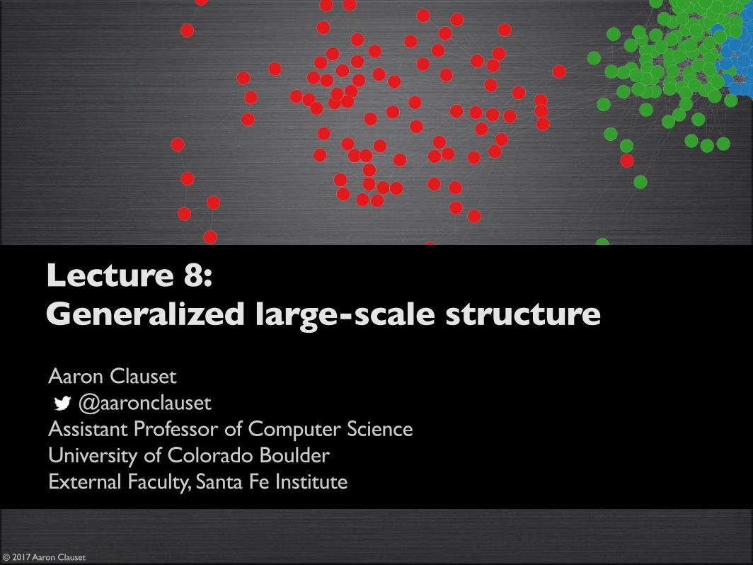
y)• 2nd order phase transition

in detectability• overlap goes to 0 for

✏ � c�pc

c+pc(k � 1)



• for 2 groups, phase transition is information theoreticno algorithm can exist that detects these communities (better than chance)

• when communities are strong, most algorithms succeed• when networks & communities are very sparse = trouble

• recently generalized to dynamic networks (Ghasemian et al. 2015)• hierarchical block models (Peixoto 2014) and node metadata (Newman &

Clauset 2016) both improve detectability

Decelle, Krzakala, Moore, & Zdeborová, Phys. Rev. Lett. 107, 065701 (2011)Ghasemian et al., arxiv:1506.0679 (2015)Peixoto, Phys. Rev. X 4, 011047 (2014)Newman & Clauset, Nature Communications, to appear (2016)

the trouble with community detection


many networks include metadata on their nodes:

metadata is often used to evaluate the accuracy of community detection algs.

if community detection method finds a partition that correlates with then we say that is good

social networks age, sex, ethnicity or race, etc.

food webs feeding mode, species body mass, etc.

Internet data capacity, physical location, etc.

protein interactions molecular weight, association with cancer, etc.

x

P xAA


1

2

3

4

5

6

7

8

9

10

11

12

13

14

15

16

17

18

19

20

21

22

23

24

25 26

27

28

29

30

31

32

33

34

Zachary karate club political blogs network


0

1

2

3

4

5

6

78

9

10

11

1213

14

15

16

17

18

19

20

21

22

23

24

25

26

27

28

29

30

31

32

33

34

35

36

37

38

3940

41

42

43

44

45

46

47

48

49

50

51

52

53

54

55

56

57

58

59

60

61

62

63

64

65

66

67

68

69

70

71

72

73

74

75

76

77

78

79

80

81

82

83

84

85

86

87

88

89

90

91

92

93

94

95 96

97

98

99

101

102

103

104

105

106

107

108

109 110

111

112

113

114

100

NCAA 2000 Schedule

political books (2004)


often, groups found by community detection are meaningful

• allegiances or personal interests in social networks [1]

• biological function in metabolic networks [2]

but

[1] see Fortunato (2010), and Adamic & Glance (2005)[2] see Holme, Huss & Jeong (2003), and Guimera & Amaral (2005)


often, groups found by community detection are meaningful

• allegiances or personal interests in social networks [1]

• biological function in metabolic networks [2]

but some recent studies claim these are the exception

• real networks either do not contain structural communities or communities exist but they do not correlate with metadata groups [3]

[1] see Fortunato (2010), and Adamic & Glance (2005)[2] see Holme, Huss & Jeong (2003), and Guimera & Amaral (2005)[3] see Leskovec et al. (2009), and Yang & Leskovec (2012), and Hric, Darst & Fortunato (2014)


Hric, Darst & Fortunato (2014)

• 115 networks with metadata & 12 community detection methods

• compare extracted with observed for each 3

Name No. Nodes No. Edges No. Groups Description of group nature

lfr 1000 9839 40 artificial network (lfr, 1000S, µ = 0.5)

karate 34 78 2 membership after the split

football 115 615 12 team scheduling groups

polbooks 105 441 2 political alignment

polblogs 1222 16782 3 political alignment

dpd 35029 161313 580 software package categories

as-caida 46676 262953 225 countries

fb100 762–41536 16651–1465654 2–2597 common students’ traits

pgp 81036 190143 17824 email domains

anobii 136547 892377 25992 declared group membership

dblp 317080 1049866 13472 publication venues

amazon 366997 1231439 14–29432 product categories

flickr 1715255 22613981 101192 declared group membership

orkut 3072441 117185083 8730807 declared group membership

lj-backstrom 4843953 43362750 292222 declared group membership

lj-mislove 5189809 49151786 2183754 declared group membership

Table I: Basic properties of all datasets used in this analysis. fb100 consists of 100 unique networks of universities, so weshow the ranges of the number of nodes and edges of the networks, as well as of the metadata groups of the various partitions.amazon consists of a hierarchical set of 11 group levels, we report the range of the number of groups. The number of groups iscalculated after our indicated preprocessing (see text).

Ganxis [29] (formerly SLPA) is based on label propaga-tion. GreedyCliqueExp [30] begins with small cliques asseeds and expands them optimizing a local fitness func-tion.

III. STRUCTURAL PROPERTIES OF NODEGROUPS FROM METADATA

Here we show some basic topological features of themetadata groups of our datasets. Fig. 1 reports thedistribution of the group sizes, which is skewed for alldatasets. Power law fits of the tails deliver exponentsaround �2. This is in agreement with the behavior ofthe size distributions for the communities found by com-munity detection algorithms on real networks [1].

The link density of a subgraph S is the ratio betweenthe number of links joining pairs of nodes of S and the to-tal maximum number of links that could be there, whichis given by nS(nS � 1)/2, nS being the number of nodesof S. In Fig. 2 we see the link density of the metadatagroups versus their sizes. Clearly, the larger the size ofthe group, the lower the link density. This is becausereal graphs are typically sparse, so the total number oflinks scales linearly with the number of nodes. This holdsfor parts of the network too, modulo small variations, sothe link density decreases approximately as a power ofthe number of links of the group (with exponent close to�1). Since the latter is proportional to the group size,we obtain that the link density decreases as the inverseof the group size, as we see in Fig. 2.

Finally, in Fig. 3 we report the relation between thegroup embeddedness and its size. The embeddedness of

Figure 1: (Color online) Distribution of sizes of metadatagroups. Each curve corresponds to a specific dataset of ourcollection.

a group is the ratio between the internal degree of thegroup and the total degree. The internal degree of agroup is given by the sum of the internal degrees of thegroup’s nodes, i.e. twice the number of links inside thegroup. The total degree of the group is the sum of thedegrees of its nodes. A group is “good” if it has highembeddedness, i.e. if it is well separated from (looselyconnected to) the rest of the graph. We notice that someof the datasets of our collection have groups with fairly

P x A

[1] fb100 is 100 networks


Hric, Darst & Fortunato (2014)

• evaluate by normalized mutual information6

Figure 5: (Color online) NMI scores between structural communities and metadata groups for di↵erent networks. Scores aregrouped by datasets on the x -axis. The height of each column is the maximal NMI score between any partition layer of themetadata partitions and any layer returned by the community detection method, considering only those comparisons wherethe overlap of the partitions is larger than 10% of total number of nodes.

methods do not align with partitions built from meta-data, but what about specific groups? Can we detectany of the groups well? Are some groups reflected in thegraph structure and detectable, but lost in the bulk noiseof the graph? This is what we wish to investigate here.

The basis of our analysis is the Jaccard score betweentwo groups. Let Ci represent (the set of nodes of) theknown group i, and Dj represent (the set of nodes of)the detected community j. The Jaccard score betweenthese two sets is defined as

J(Ci, Dj) =|Ci \Dj ||Ci [Dj |

, (1)

with |· · · | set cardinality, \ set intersection, and [ setunion. The Jaccard score ranges from one (perfectmatch) to zero and roughly indicates the fraction of nodesshared between the two sets: the match quality.

The recall score measures how well one known group isdetected. The recall score of one known group Ci is de-fined as the maximal Jaccard score between it and everydetected community Dj ,

R(Ci) = maxDj2{D}

J(Ci, Dj). (2)

It is near one if the group is well detected and low oth-erwise. We can study the distribution of these scores tosee how many groups can be detected at any given qual-ity level. Recall measures the detection of known groups,and to measure the significance of detected communities,we can reverse the measure to calculate a precision score

P (Dj) = maxCi2{C}

J(Dj , Ci). (3)

The precision score tells us how well one detected com-munity corresponds to any known group.

We can now directly quantify the two conditions forgood community detection: every known group must cor-respond to some detected community, and every detectedcommunity must represent some known group. Both ofthese measures are still interesting independently: a highrecall but low precision indicates that the known groupsare reflected in the network structurally, but there aremany structural communities that are not known. Wevisualize the scores by means of rank-Jaccard plots whichgive an overview of the network’s detection quality. Wecompute the recall (precision) for every known (detected)group and sort the groups in order of ascending Jaccardscore. We plot recall (precision) vs the group rank, sortedby recall (precision) score so that the horizontal scale isthe relative group rank, i.e. the ratio between the rank ofthe group and the number of groups (yielding a value be-tween 0 and 1). Similar to our treatment of the partition-level analysis, we only plot matchings whose intersectioncovers more than 10% of total nodes in the graph. In ourfinal plots, the average value of the curve (proportional tothe area under it) is the average recall or precision scoreover all groups. The shape of the curve can tell us if allgroups are detected equally well (yielding a high plateau)or if there is a large inequality in detection (a high slope).Furthermore, this allows us to compactly represent mul-tiple layers. Each independent layer of known (detected)groups can be plotted in the same figure. We would gen-erally look for the highest curve to know if any layer hasa high recall (precision). When computing recall (preci-sion), unless otherwise specified, as detected communitieswe consider the communities of all partitions delivered bya method, whereas the metadata groups are those presentin all metadata partitions (if more than one partition isavailable in either case). This will give us the maximumpossible recall (precision), which might be far higher than

NMI(P,x)

[1] maximum NMI between any partition layer of the metadata partitions and any layer returned by the community detection method

{ "classic" data sets

but wait!

[1] image copyright BostonGazette or maybe 20th Century Fox? gah

a solution

idea: use metadata to help select a partition that correlates with , from among the exponential number of plausible partitions

P⇤ 2 {P}x x

[1] image copyright BostonGazette or maybe 20th Century Fox? gah

idea: use metadata to help select a partition that correlates with , from among the exponential number of plausible partitions

use a generative model to guide the selection:• define a parametric probability distribution over networks

• generation : given , draw from this distribution

• inference : given , choose that makes likely

P⇤ 2 {P}

a solution

Pr(G | ✓)✓ G

G ✓ G

x x

generation

inference

model

G=(V,E)

data

Pr(G | θ)

generation

given metadata and degree for each node • each node is assigned a community with probability

• thus, prior on community assignments is

• given assignments, place edges independently, each with probability:

• where the are the stochastic block matrix parameters

this is a degree-corrected stochastic block model (DC-SBM)with a metadata-based prior on community labels

a metadata-aware stochastic block model

x = {xu} d = {du}�sx

su

u

P (s |�,x) =Y

i

�si,xi

[1] is the matrix of parameters [2] Karrer & Newman (2011)

� k ⇥K �sx

puv = dudv✓su,sv✓st

P (A |⇥,�,x) =X

s

P (A |⇥, s)P (s |�,x)

=X

s

Y

u<v

pAuvuv

(1� puv

)1�AuvY

u

�su,xu

inference

given observed network (adjacency matrix)• the model likelihood is

• where is a matrix of community interaction parameters , and the sum is over all possible assignments

• we fit this model to data using expectation-maximization (EM) to maximize w.r.t. and

a metadata-aware stochastic block model

A

⇥ ✓stk ⇥ ks

P (A |⇥,�,x) ⇥ �

[1] technical details in Newman & Clauset (2015) arxiv:1507.04001

network metadata

http://arxiv.org/abs/1507.04001

networks with planted structure

does this method recover known structure in synthetic data?


does this method recover known structure in synthetic data?

• use SBM to generate planted partition networks, with equal-sized groups and mean degree

• assign metadata with variable correlation to true group labels

• vary strength of partition

k = 2

⇢ 2 [0.5, 0.9]

cin

� cout

c = (cin

+ cout

)/2

cin

� cout

p

2(cin

+ cout

)

[1] Decelle, Krzakala, Moore & Zdeborova (2011)

cout

n

cinn

cinn

cout

n

• when , no structure-only algorithm can recover the planted communities better than chance (the detectability threshold, which is a phase transition)

cin-cout

0 1 2 3 4 5 6 7 8 9 10 11 12 13 14 15

Frac

tion

of c

orre

ctly

ass

igne

d no

des

0.5

0.55

0.6

0.65

0.7

0.75

0.8

0.85

0.9

0.95

1 0.50.60.70.80.9


undetectable

let mean degree • when , metadata isn’t useful and we recover regular SBM behavior

c = 8

⇢ = 0.5

[1] n = 10 000

weaker stronger


cin-cout

0 1 2 3 4 5 6 7 8 9 10 11 12 13 14 15

Frac

tion

of c

orre

ctly

ass

igne

d no

des

0.5

0.55

0.6

0.65

0.7

0.75

0.8

0.85

0.9

0.95

1 0.50.60.70.80.9

• when metadata correlates with true groups, accuracy is better than either metadata or SBM alone

metadata + SBM performs better than either

• any algorithm without metadata, or

• metadata alone.

let mean degree • when , metadata isn’t useful and we recover regular SBM behavior⇢ = 0.5

⇢ > 0.5

c = 8

undetectable

weaker stronger

real-world networks

real-world networks

1. high school social network: 795 students in a medium-sized American high school and its feeder middle school

2. marine food web: predator-prey interactions among 488 species in Weddell Sea in Antarctica

3. Malaria gene recombinations: recombination events among 297 var genes

4. Facebook friendships: online friendships among 15,126 Harvard students and alumni

5. Internet graph: peering relations among 46,676 Autonomous Systems

real-world networks


• {grade 7-12, ethnicity, gender}x =

[1] Add Health network data, designed by Udry, Bearman & Harris

real-world networks



• method finds a good partition between high-school and middle-school

• .

• without metadata:

NMI = 0.881


NMI 2 [0.105, 0.384]

real-world networks



• method finds a good partition between blacks and whites (with others scattered among)


NMI = 0.820

NMI 2 [0.120, 0.239]


real-world networks



• method finds no good partition between males/females. instead, chooses a mixture of grade/ethnicity partitions


NMI = 0.003

NMI 2 [0.000, 0.010]


real-world networks

2. marine food web: predator-prey interactions among 488 species in Weddell Sea in Antarctica

• {species body mass, feeding mode, oceanic zone}

• partition recovers known correlation between body mass, trophic level, and ecosystem role:

x =

1

2

3

Detritivore

Carnivore

Omnivore

Herbivore

Primary producer[1] here, we’re using a continuous metadata model[2] Brose et al. (2005)

8

(a) Without metadata

(b) With metadata

FIG. S3: Inferred communities, without metadata and with,for the HVR 5 gene recombination network of the humanmalaria parasite P. falciparum, where metadata values arethe CP labels for the HVR 6 network.

predictive (96% probability) of that gene being in onegroup, while having four cysteines is modestly predictive(67% probability) of being in the other group. Thus themethod has discovered by itself that the motif sequencesthat define the CP labels, along with their correspondingnetwork communities, correlate with cysteine counts andtheir associated severe disease phenotypes [8, 11].

The communities in the HVR 6 network representhighly non-random patterns of recombination, which arethought to indicate functional constraints on proteinstructure. Previous work has conjectured that commonconstraints on recombination span distinct HVRs [9]. Wecan test this hypothesis using the methods described inthis paper. There is no reason a priori to expect thatthe community structure of HVR 6 should correlate withthat of HVR 5 because the Cys and CP labels are derivedfrom outside the HVR 5 sequences—Cys labels reflectcysteine counts in HVR 6 while CP labels subdivide Cyslabels based on sequence motifs adjacent to, but outsideof, HVR 5. Applying our methods to HVR 5 withoutany metadata (Fig. S3a), we find mixing of the HVR 6Cys labels across the HVR 5 communities. By contrast,using the CP labels as metadata for the HVR 5 network,our method finds a much cleaner partition (Fig. S3b), in-dicating that indeed the HVR 6 Cys labels correlate withthe community structure of HVR 5.

10-12

10-9

10-6

10-3

100

103

106

109

Mean body mass (g)

0

0.5

1

Pro

bab

ilit

y o

f co

mm

un

ity

mem

ber

ship

FIG. S4: Learned priors, as a function of body mass, for thethree-community division of the Weddell Sea network shownin Fig. 4 of the main paper.

C. Weddell Sea food web

As discussed in the main text, the Weddell Sea foodweb provides an example of the “ordered” metadata typein the body mass of species. A three-way community di-vision of the network with the log of species’ averagebody mass as metadata produces the division shown inFig. 4 of the paper. The prior probabilities as functionsof body mass are of interest in their own right. They areshown in Fig. S4. Although, as described in Section ICof the paper, the log mass is rescaled in our calculationsto the range [0, 1], the horizontal axis in the figure is cal-ibrated to read in terms of the original mass in grams, sothe prior probabilities of belonging to each of the threecommunities can be simply read from the figure. Theblue, green, and red curves correspond respectively tothe communities labeled 1, 2, and 3 in Fig. 4. Thus aspecies with a low mean mass of 10�12 g has about an80% probability of being in community 1, a 20% proba-bility of being in community 2, and virtually no chance ofbeing in community 3. Conversely, a species with meanbody mass of 108 g (which could only be a whale) hasabout a 90% chance of being in community 3, 10% ofbeing in community 2, and almost no chance of being incommunity 1.

D. School friendship network data use

Our use of the school friendship data described in themain text requires that we make the following statement:

This work uses data from Add Health, a pro-gram project designed by J. Richard Udry,Peter S. Bearman, and Kathleen Mullan Har-ris, and funded by a grant P01–HD31921from the National Institute of Child Health

3

2

1

real-world networks

x =

[1] Larremore, Clauset & Buckee (2013)


• {Cys-PoLV labels for HVR6 region}

• with metadata, partition discovers correlation with Cys labels (which are associated with severe disease)

without metadata with metadata

HVR6

NMI 2 [0.077, 0.675] NMI = 0.596

real-world networks

x =

[1] Larremore, Clauset & Buckee (2013)


• {Cys-PoLV labels for HVR6 region}

• on adjacent region of gene, we find Cys-PoLV labels correlate with recombinant structure here, too

HVR5

without metadata with metadata

the ground truth about metadata

what is the goal of community detection?

network + method communities vs. metadataC = f(G) MG f !




"this method works!"

C ⇡ M




"this method works!" "this method stinks!"

C ⇡ M C 6= M



there are 4 indistinguishable reasons why we might find :

1. metadata are unrelated to network structure

f(G) = C 6= M

M G





2. metadata and communities capture different aspects of structure

social groups leaders and followers

M

C

G

M

f(G) = C 6= M






3. network has no community structure

M

C

G

M

G

f(G) = C 6= M






3. network has no community structure

4. algorithm is bad

"this method stinks!"

M

C

G

M

G

f

f(G) = C 6= M

DON’T TRY TO FIND THE GROUND TRUTH

INSTEAD . . . TRY TO REALIZE THERE IS NO GROUND TRUTH

theorems for community detection

theorems for community detection

1. Theorem: no bijection between ground truth and communities

2. Theorem: No Free Lunch in community detection

g(T )! G g0(T 0) 2 different processes, on 2 different ground truths, can create the same observed network

no algorithm has better performance than any other algorithm , when averaged over all possible inputs

good performance comes from matching algorithm to its preferred subclass of networks

[1] performance defined as adjusted mutual information (AMI), which is like the normalized mutual information, but adjusted for expected values[2] original NFL theorem: Wolpert, Neural Computation (1996)[3] proofs of these theorems is in Peel, Larremore, Clauset (2016)

ff 0

{G}

!f{G0} ⇢ {G}

fin

real-world networks

x =

[1] Traud, Mucha & Porter (20012)

13

communities is less than the number of metadata values,in some cases by a wide margin. Assuming the values ofboth to be reasonably broadly distributed, this impliesthat the entropy H(s) of the communities will be smallerthan that of the metadata H(x) and hence, normally,min[H(s), H(x)] = H(s). Thus if we define

NMI =I(s ;x)

min[H(s), H(x)], (B4)

we ensure that the normalized mutual information liesbetween zero and one, that it has a symmetric defini-tion with respect to s and x, and that it will achieveits maximum value of one when the metadata perfectlypredict the community membership. Other definitions,normalized using the mean or maximum of the two en-tropies, satisfy the first two of these three conditions butnot the third, giving values smaller than one by an unpre-dictable margin even when the metadata perfectly pre-dict the communities.We use the definition (B4) in all the calculations pre-

sented in this paper.

Appendix C: Further examples

In this appendix we present a number of additionalapplications of our methods as well as some additionaldetails on examples described in the main text. Summarystatistics on all the networks studied are given in Table I.

1. Facebook friendship network

The FB100 data set of Traud et al. [31] is a set offriendship networks among college students at US uni-versities compiled from friend relations on the social net-working website Facebook. The networks date from theearly days of Facebook when its services were availableonly to college students and each university formed a sep-arate and unconnected subgraph in the larger network.The nodes in these networks represent the students, theedges represent friend relations on Facebook, and in ad-dition to the network structure there are metadata ofseveral types, including gender, college year (i.e., yearof college graduation), major (i.e., principal subject ofstudy, if known), and a numerical code indicating whichdorm they lived in.The primary divisions in these networks appear to be

by age, or more specifically by college year. For instance,we have looked in some detail at the data for HarvardUniversity, which was the birthplace of Facebook andits biggest institutional participant at the time the datawere gathered, with 15 126 students in the network, span-ning college years 2003 to 2009. There are also a smallnumber of Harvard alumni (i.e., former students) in thedata set, primarily those recently graduated—graduationyears 2000–2002. The top panel in Fig. 4 shows results

None 2000 2001 2002 2003 2004 2005 2006 2007 2008 2009

Year

0

0.5

1Pr

ior p

roba

bilit

y of

mem

bers

hip

Dorm0

0.5

1

Prio

r pro

babi

lity

of m

embe

rshi

p

FIG. 4: Learned prior probability of community membershipfor two five-way divisions of the Facebook friendship networkof Harvard students described in the text. The horizontal axisis (top) year of graduation and (bottom) dorm, and the colorsrepresent the prior probabilities of membership in each of thecommunities.

from a five-way division of the network using our algo-rithm with year as metadata. Year, for the purposes ofthis calculation, was treated as an unordered variable,placing no constraints on the value of the prior probabil-ities of community membership for adjacent years. Onecould have treated it as an ordered variable, which wouldhave constrained adjacent years to have similar priors,but we did not do that here. Nonetheless, as we will see,the algorithm finds communities in which adjacent yearstend to be grouped together.This network provides a good example of the useful-

ness of the learned priors in shedding light on the struc-ture of the network. The figure shows a visualization ofthe priors as a function of year, with the colors show-ing the relative probability of belonging to each of thecommunities. Each of the bars in the plot has the sameheight of 1 since the prior probabilities are required tosum to 1, while the balance of colors shows the distribu-tion over communities. Examination of the top panel inthe figure shows clearly a division of the network alongage lines. Two groups, in orange and yellow at the rightof the plot, correspond to the most recent two years ofstudents at the time of the study (graduation years 2008and 2009) and the next, in red, accounts for the two yearsbefore that (2006 and 2007). The purple community cor-responds to the next three years, 2003–2005, while the

NMI 2 [0.573, 0.641]

NMI = 0.668

4. Facebook friendships: online friendships among 15,126 Harvard students and alumni (in Sept. 2005)

• {graduation year, dormitory}

• method finds a good partition between alumni, recent graduates, upperclassmen, sophomores, and freshmen

• .


real-world networks

x =

[1] Traud, Mucha & Porter (20012)

4. Facebook friendships: online friendships among 15,126 Harvard students and alumni (in Sept. 2005)

• {graduation year, dormitory}

• method finds a good partition among the dorms

• .


13

communities is less than the number of metadata values,in some cases by a wide margin. Assuming the values ofboth to be reasonably broadly distributed, this impliesthat the entropy H(s) of the communities will be smallerthan that of the metadata H(x) and hence, normally,min[H(s), H(x)] = H(s). Thus if we define

NMI =I(s ;x)

min[H(s), H(x)], (B4)

we ensure that the normalized mutual information liesbetween zero and one, that it has a symmetric defini-tion with respect to s and x, and that it will achieveits maximum value of one when the metadata perfectlypredict the community membership. Other definitions,normalized using the mean or maximum of the two en-tropies, satisfy the first two of these three conditions butnot the third, giving values smaller than one by an unpre-dictable margin even when the metadata perfectly pre-dict the communities.We use the definition (B4) in all the calculations pre-

sented in this paper.

Appendix C: Further examples

In this appendix we present a number of additionalapplications of our methods as well as some additionaldetails on examples described in the main text. Summarystatistics on all the networks studied are given in Table I.

1. Facebook friendship network

The FB100 data set of Traud et al. [31] is a set offriendship networks among college students at US uni-versities compiled from friend relations on the social net-working website Facebook. The networks date from theearly days of Facebook when its services were availableonly to college students and each university formed a sep-arate and unconnected subgraph in the larger network.The nodes in these networks represent the students, theedges represent friend relations on Facebook, and in ad-dition to the network structure there are metadata ofseveral types, including gender, college year (i.e., yearof college graduation), major (i.e., principal subject ofstudy, if known), and a numerical code indicating whichdorm they lived in.The primary divisions in these networks appear to be

by age, or more specifically by college year. For instance,we have looked in some detail at the data for HarvardUniversity, which was the birthplace of Facebook andits biggest institutional participant at the time the datawere gathered, with 15 126 students in the network, span-ning college years 2003 to 2009. There are also a smallnumber of Harvard alumni (i.e., former students) in thedata set, primarily those recently graduated—graduationyears 2000–2002. The top panel in Fig. 4 shows results

None 2000 2001 2002 2003 2004 2005 2006 2007 2008 2009

Year

0

0.5

1

Prio

r pro

babi

lity

of m

embe

rshi

p

Dorm0

0.5

1Pr

ior p

roba

bilit

y of

mem

bers

hip

FIG. 4: Learned prior probability of community membershipfor two five-way divisions of the Facebook friendship networkof Harvard students described in the text. The horizontal axisis (top) year of graduation and (bottom) dorm, and the colorsrepresent the prior probabilities of membership in each of thecommunities.

from a five-way division of the network using our algo-rithm with year as metadata. Year, for the purposes ofthis calculation, was treated as an unordered variable,placing no constraints on the value of the prior probabil-ities of community membership for adjacent years. Onecould have treated it as an ordered variable, which wouldhave constrained adjacent years to have similar priors,but we did not do that here. Nonetheless, as we will see,the algorithm finds communities in which adjacent yearstend to be grouped together.This network provides a good example of the useful-

ness of the learned priors in shedding light on the struc-ture of the network. The figure shows a visualization ofthe priors as a function of year, with the colors show-ing the relative probability of belonging to each of thecommunities. Each of the bars in the plot has the sameheight of 1 since the prior probabilities are required tosum to 1, while the balance of colors shows the distribu-tion over communities. Examination of the top panel inthe figure shows clearly a division of the network alongage lines. Two groups, in orange and yellow at the rightof the plot, correspond to the most recent two years ofstudents at the time of the study (graduation years 2008and 2009) and the next, in red, accounts for the two yearsbefore that (2006 and 2007). The purple community cor-responds to the next three years, 2003–2005, while the

NMI 2 [0.074, 0.224]

NMI = 0.255

Documents

Lecture 8: Generalized large-scale structuretuvalu.santafe.edu/~aaronc/courses/5352/csci5352_2017_L8.pdf · Aaron Clauset @aaronclauset Assistant Professor of Computer Science University