Lecture 6:Securing Distributed and Networked

Systems

CS 598: Network Security

Matthew Caesar

March 12, 2013

1

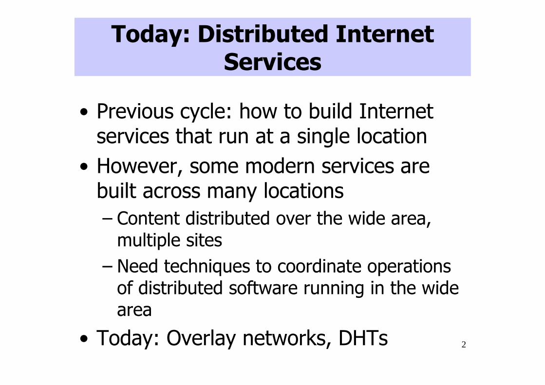
Today: Distributed Internet Services

• Previous cycle: how to build Internet services that run at a single location

• However, some modern services are built across many locations

– Content distributed over the wide area, multiple sites

– Need techniques to coordinate operations of distributed software running in the wide area

• Today: Overlay networks, DHTs 2

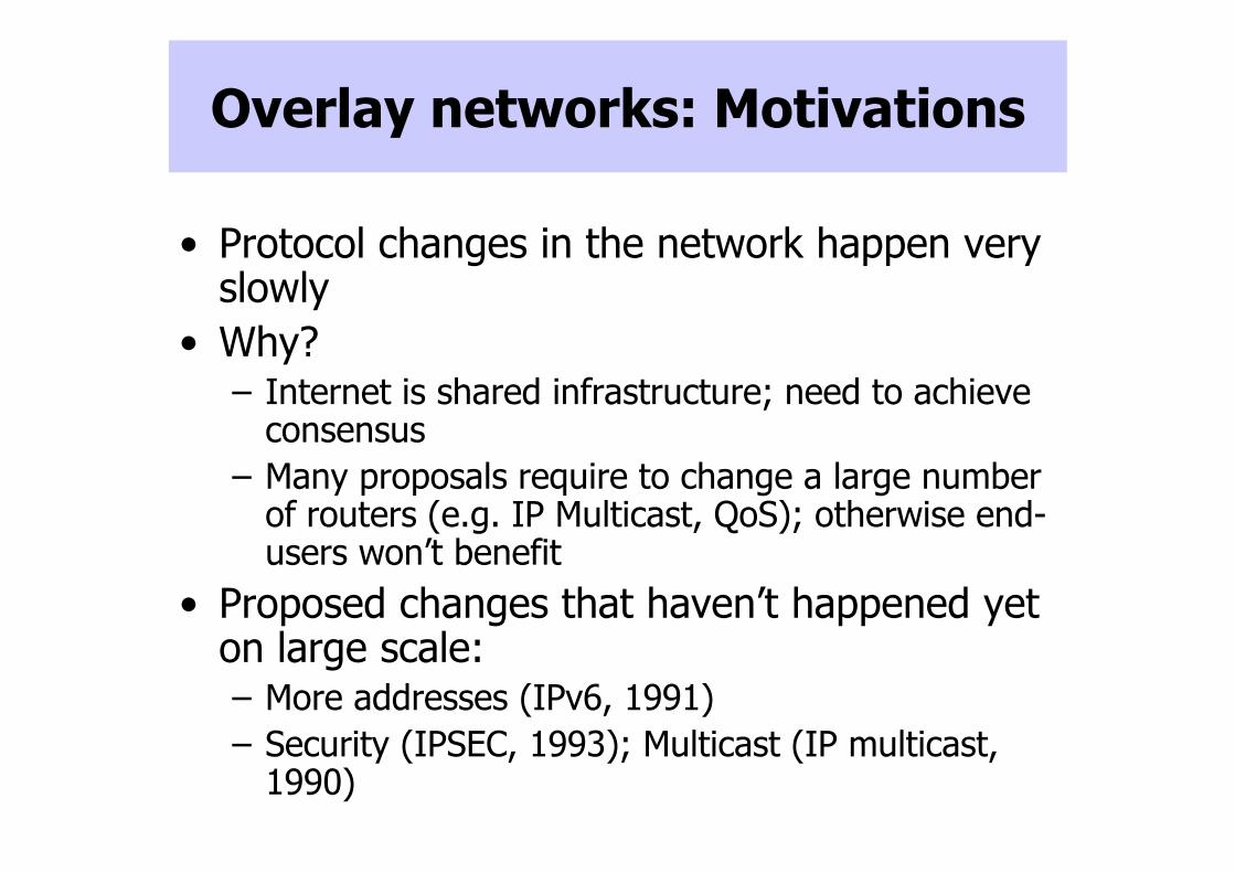
Overlay networks: Motivations

• Protocol changes in the network happen very slowly

• Why?– Internet is shared infrastructure; need to achieve

consensus

– Many proposals require to change a large number of routers (e.g. IP Multicast, QoS); otherwise end-users won’t benefit

• Proposed changes that haven’t happened yet on large scale:– More addresses (IPv6, 1991)

– Security (IPSEC, 1993); Multicast (IP multicast, 1990)

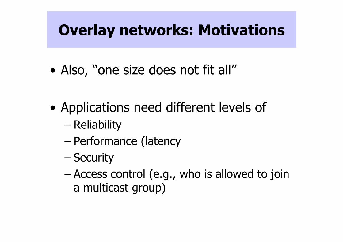
Overlay networks: Motivations

• Also, “one size does not fit all”

• Applications need different levels of

– Reliability

– Performance (latency

– Security

– Access control (e.g., who is allowed to join a multicast group)

Overlay networks: Goals

• Make it easy to deploy new functionalities in the network �

Accelerate the pace of innovation

• Allow users to customize their service

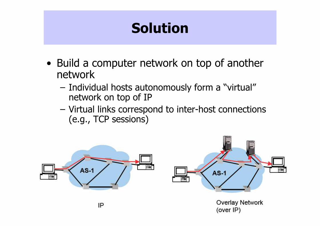
Solution

• Build a computer network on top of another network– Individual hosts autonomously form a “virtual”

network on top of IP

– Virtual links correspond to inter-host connections (e.g., TCP sessions)

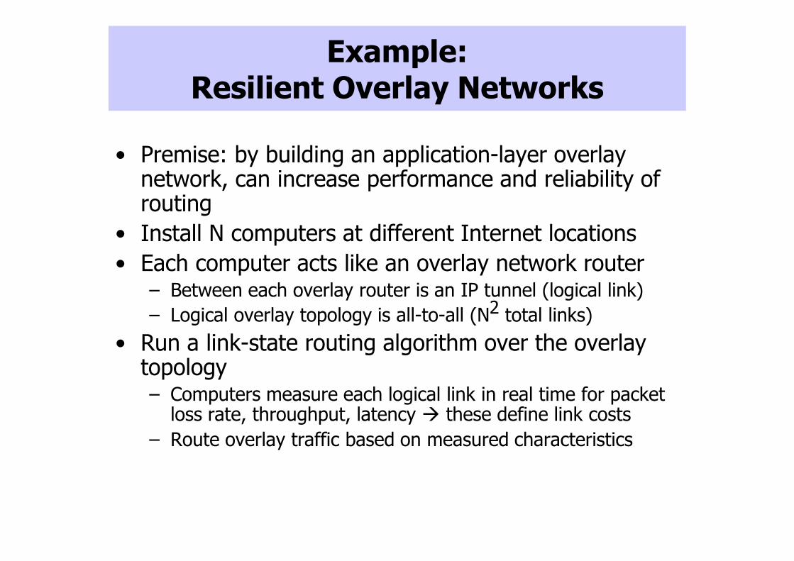
Example: Resilient Overlay Networks

• Premise: by building an application-layer overlay network, can increase performance and reliability of routing

• Install N computers at different Internet locations

• Each computer acts like an overlay network router– Between each overlay router is an IP tunnel (logical link)

– Logical overlay topology is all-to-all (N2 total links)

• Run a link-state routing algorithm over the overlay topology – Computers measure each logical link in real time for packet

loss rate, throughput, latency � these define link costs

– Route overlay traffic based on measured characteristics

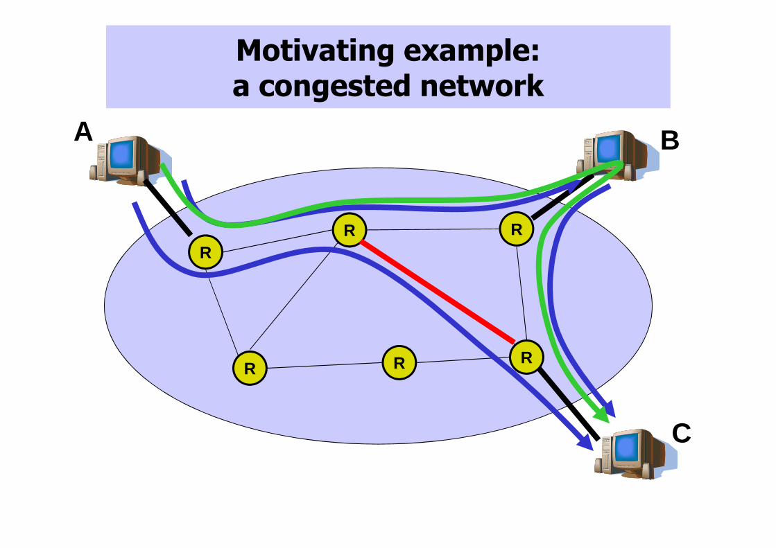
Motivating example: a congested network

R

RR

R

R

R

A B

C

Solution: an “overlay” network

R

RR

R

R

R

A B

CEstablish TCP

sessions (“overlay links”) between hosts

A B

CLoss=1%

Loss=2%

Loss=25%

Path taken by TCP sessions

Machines remember overlay

topology, probe links, advertise

link quality

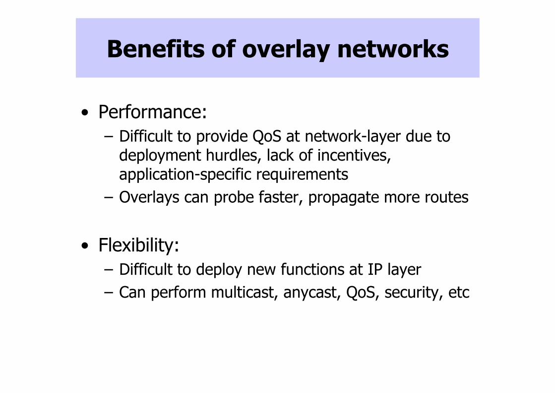
Benefits of overlay networks

• Performance:

– Difficult to provide QoS at network-layer due to deployment hurdles, lack of incentives, application-specific requirements

– Overlays can probe faster, propagate more routes

• Flexibility:

– Difficult to deploy new functions at IP layer

– Can perform multicast, anycast, QoS, security, etc

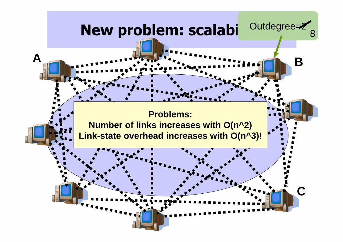
New problem: scalability

A B

C

Outdegree=28

Problems:Number of links increases with O(n^2)

Link-state overhead increases with O(n^3)!

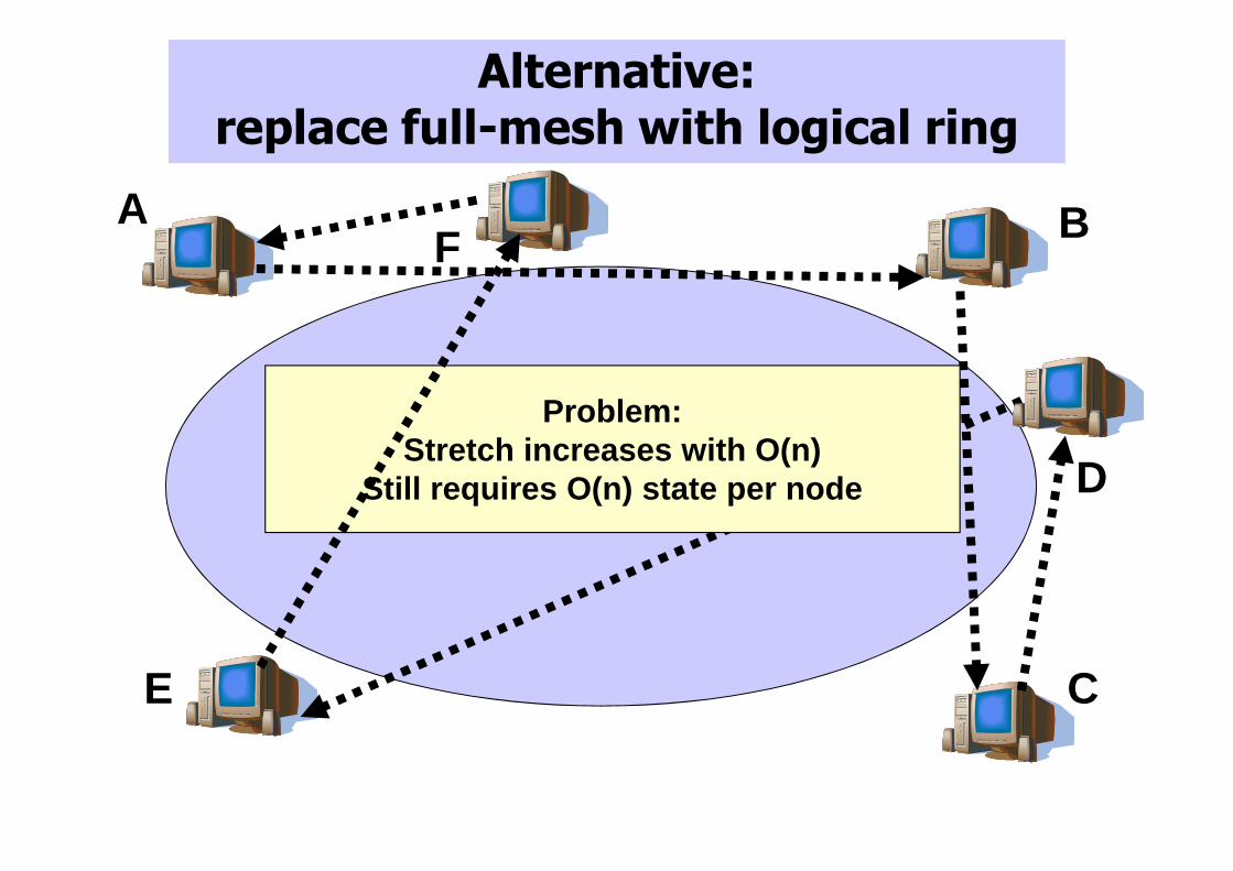
Alternative: replace full-mesh with logical ring

A B

C

Problem:Stretch increases with O(n)

Still requires O(n) state per node D

E

F

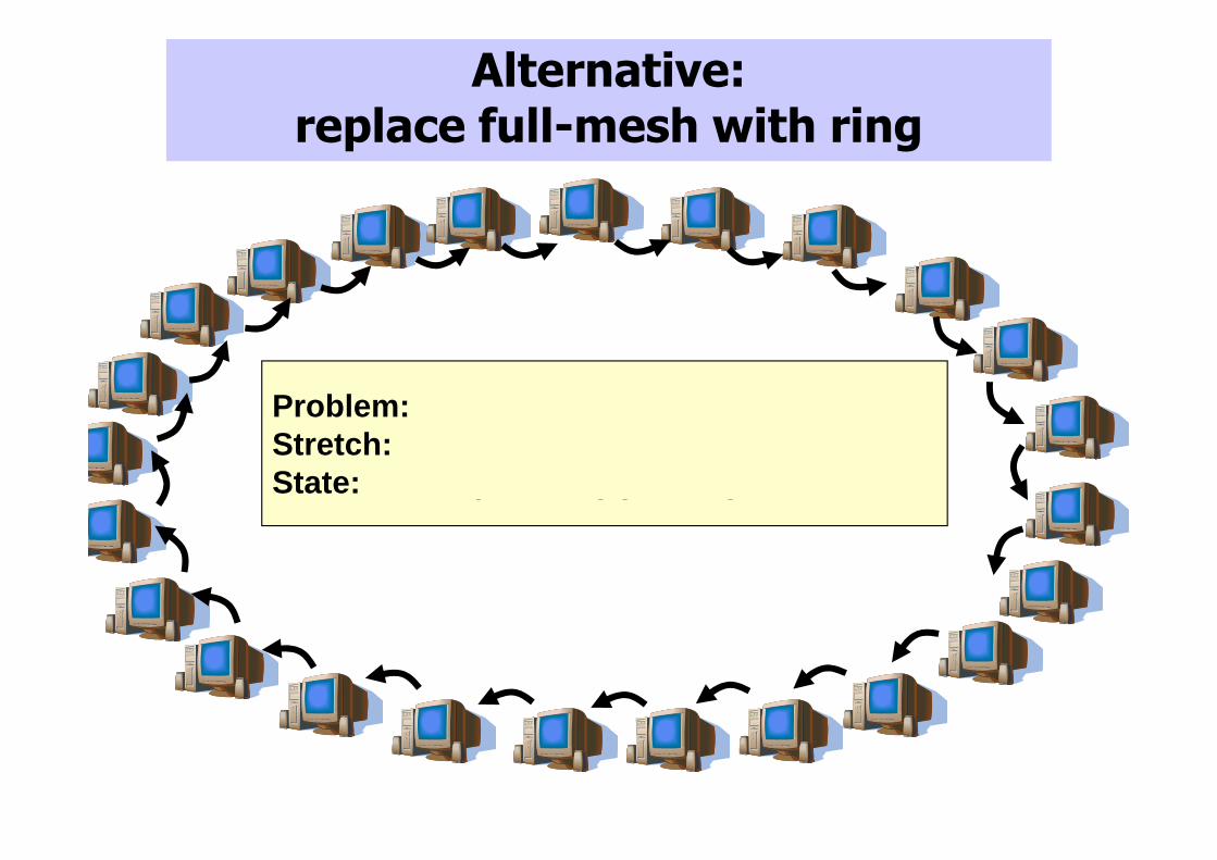
Alternative: replace full-mesh with ring

Problem:Stretch: increases with O(n)State: still requires O(n) state per node

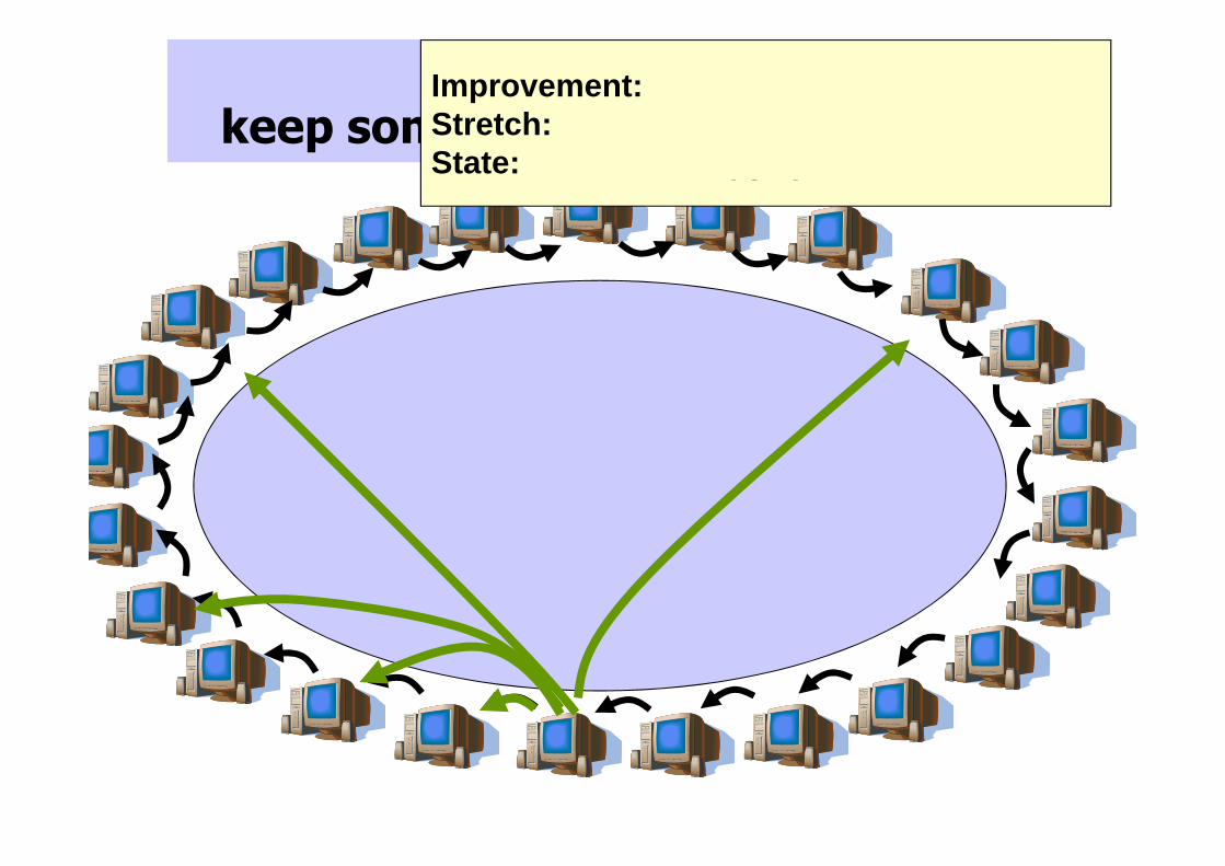
Improvement: keep some long distance pointers

Improvement:Stretch: reduces to O(lg n)State: reduces to O(lg n)

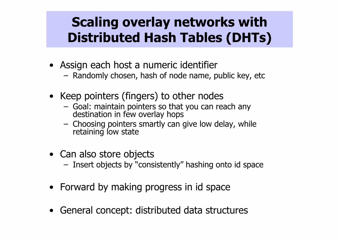
Scaling overlay networks withDistributed Hash Tables (DHTs)

• Assign each host a numeric identifier– Randomly chosen, hash of node name, public key, etc

• Keep pointers (fingers) to other nodes– Goal: maintain pointers so that you can reach any

destination in few overlay hops– Choosing pointers smartly can give low delay, while

retaining low state

• Can also store objects– Insert objects by “consistently” hashing onto id space

• Forward by making progress in id space

• General concept: distributed data structures

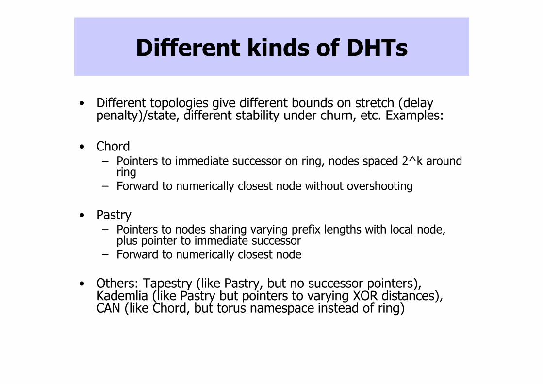
Different kinds of DHTs

• Different topologies give different bounds on stretch (delay penalty)/state, different stability under churn, etc. Examples:

• Chord– Pointers to immediate successor on ring, nodes spaced 2^k around

ring– Forward to numerically closest node without overshooting

• Pastry– Pointers to nodes sharing varying prefix lengths with local node,

plus pointer to immediate successor– Forward to numerically closest node

• Others: Tapestry (like Pastry, but no successor pointers), Kademlia (like Pastry but pointers to varying XOR distances), CAN (like Chord, but torus namespace instead of ring)

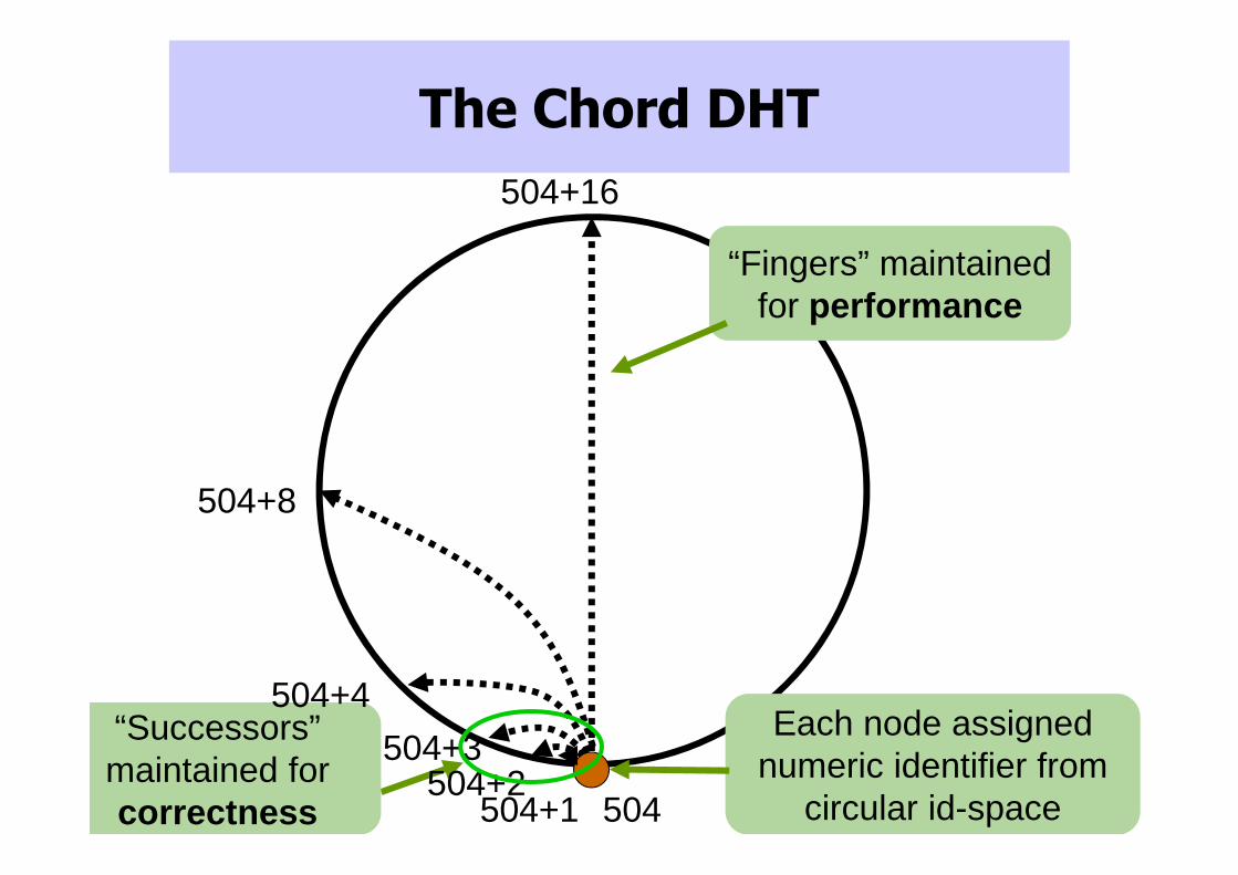
The Chord DHT

“Fingers” maintained for performance

Each node assigned numeric identifier from

circular id-space

“Successors” maintained for correctness 504504+1

504+2

504+4

504+8

504+16

504+3

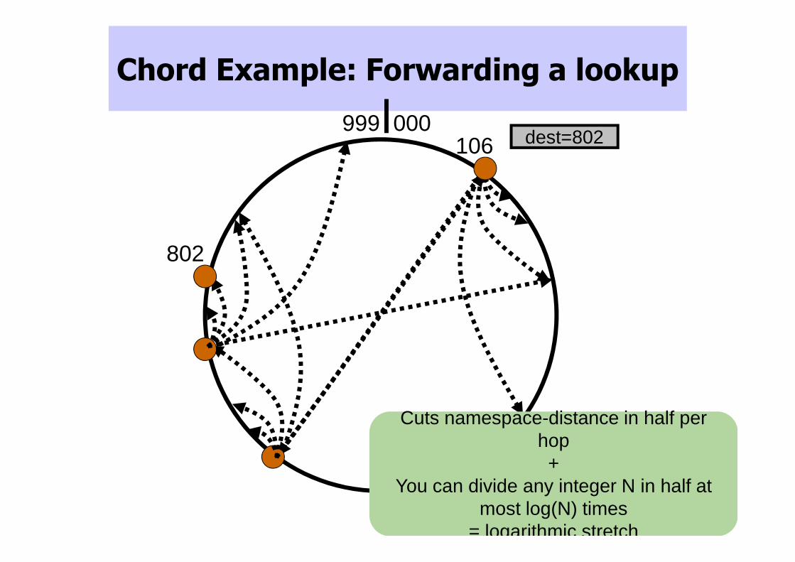
Chord Example: Forwarding a lookup

dest=802000999

106

802

Cuts namespace-distance in half per hop+

You can divide any integer N in half at most log(N) times

= logarithmic stretch

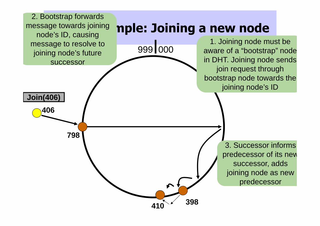
Chord Example: Joining a new node

000999

406

1. Joining node must be aware of a “bootstrap” node in DHT. Joining node sends

join request through bootstrap node towards the

joining node’s IDJoin(406)

798

2. Bootstrap forwards message towards joining

node’s ID, causing message to resolve to joining node’s future

successor

410 398

3. Successor informs predecessor of its new

successor, adds joining node as new

predecessor

Chord: Improving robustness

• To improve robustness, each node can maintain more than one successor

– E.g., maintain the K>1 successors immediately adjacent to the node

• In the notify() message, node A can send its k-1 successors to its predecessor B

• Upon receiving the notify() message, B can update its successor list by concatenating the successor list received from A with A itself

Chord: Discussion

• Query can be implemented – Iteratively

– Recursively

• Performance: routing in the overlay network can be more expensive than routing in the underlying network– Because usually no correlation between node ids

and their locality; a query can repeatedly jump from Europe to North America, though both the initiator and the node that store them are in Europe!

– Solutions: can maintain multiple copies of each entry in their finger table, choose closest in terms of network distance

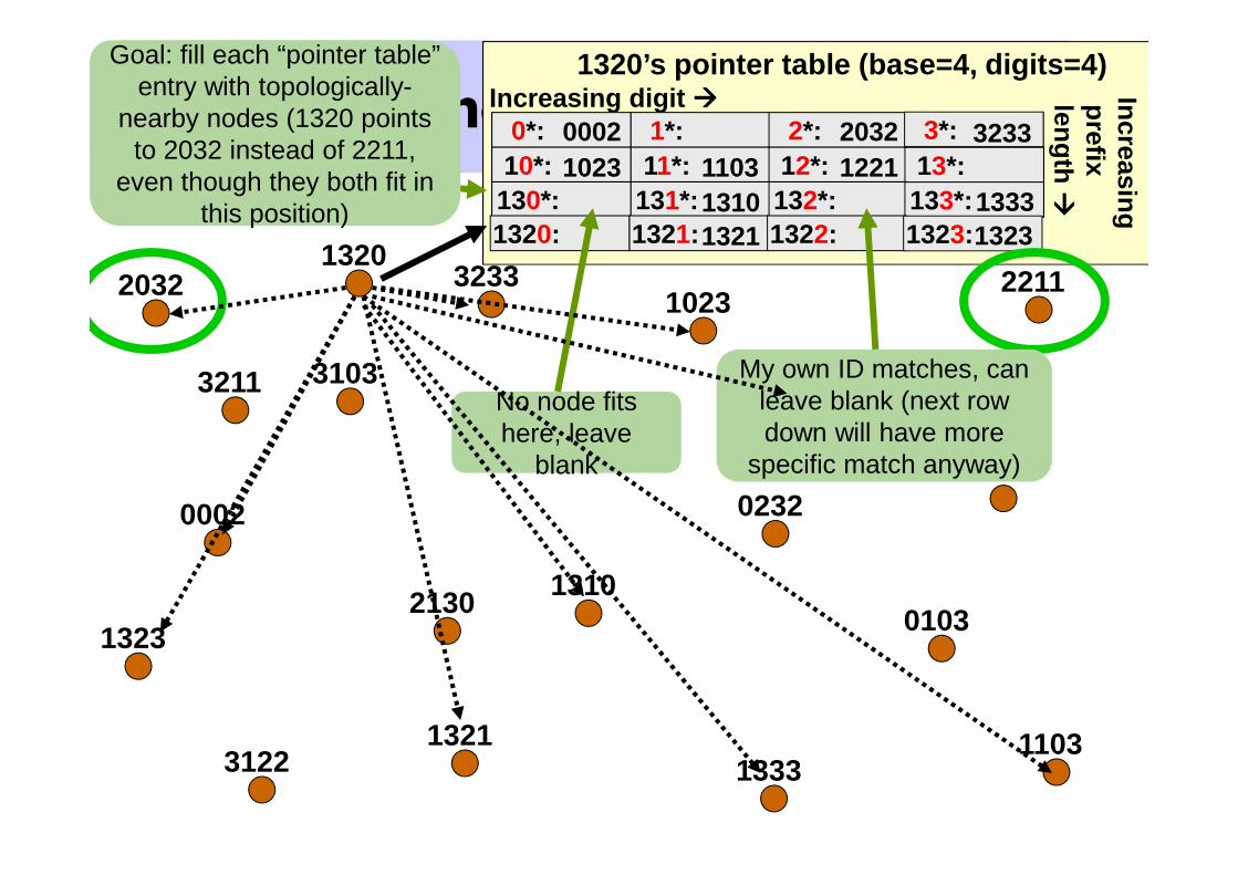
The Pastry DHT1320’s pointer table (base=4, digits=4)

Increasing digit ���� Increasin

gp

refixlen

gth

�� ��

1*: 2*: 3*: 0*: 11*: 12*: 13*:

131*: 132*: 133*: 10*: 130*:

1321: 1322: 1323: 1320: 1320

Pointers to neighbors that match my ID with varying prefix lengths,with most significant digit varied

10233233

3103

2130

1221

2211

0103

02320002

2032

13331103

3122

3211

Goal: fill each “pointer table” entry with topologically-

nearby nodes (1320 points to 2032 instead of 2211,

even though they both fit in this position)

1322

My own ID matches, can leave blank (next row down will have more

specific match anyway)

No node fits here, leave

blank

1310

2032 32331103 12211310 1333

00021023

1321 1323

1321

1323

The Pastry DHT

1320

10233233

3103

2130

1221

2211

0103

02320002

2032

13331103

3122

3211

1322

1310

1321

1323

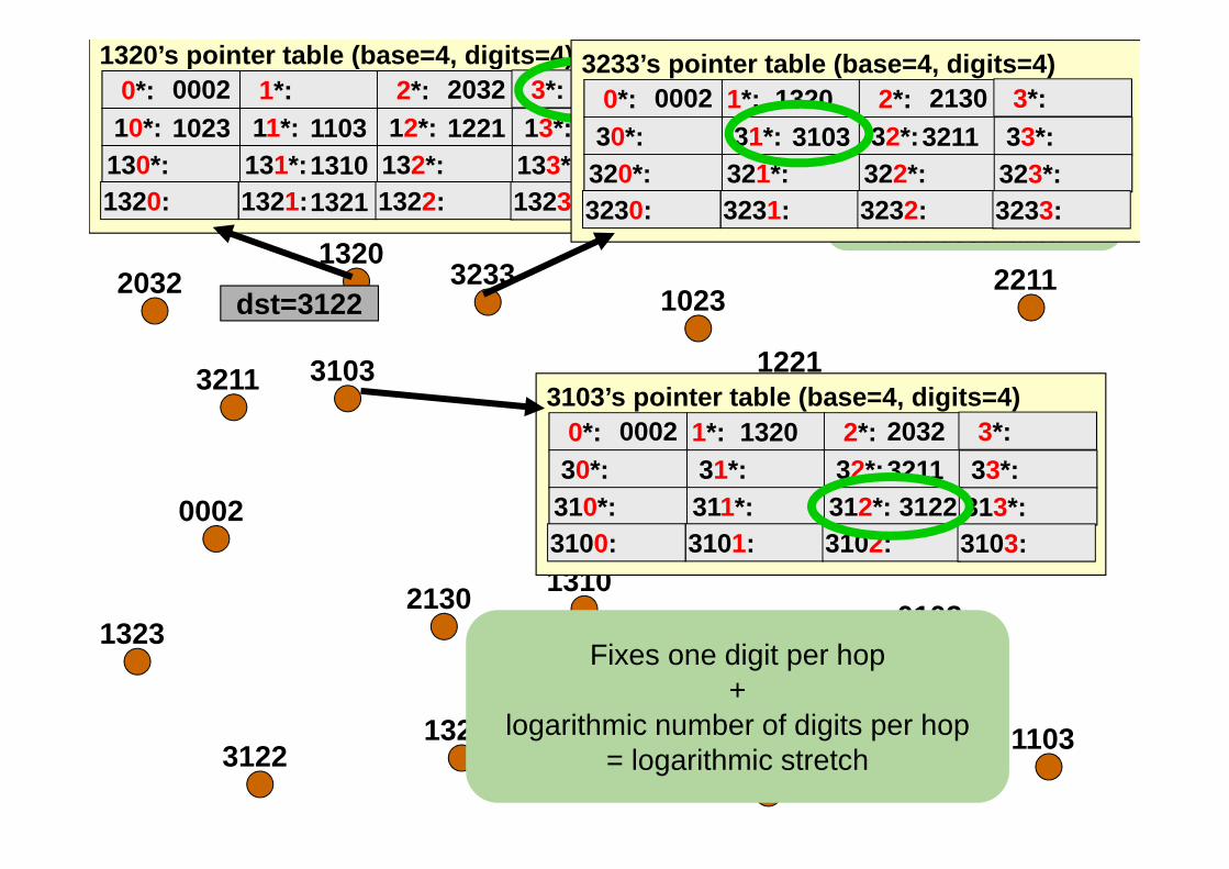
dst=3122

1320’s pointer table (base=4, digits=4)1*: 2*: 3*: 0*: 11*: 12*: 13*:

131*: 132*: 133*: 10*: 130*:

1321: 1322: 1323: 1320:

110313101321

2032 32331221

13331323

00021023 Forward to node in

table with identifier sharing longest prefix

with destination

3233’s pointer table (base=4, digits=4)1*: 1320 2*: 3*: 0*: 31*: 32*: 33*: 321*: 322*: 323*:

30*: 320*:

3231: 3232: 3233: 3230:

31032130

3211 0002

3103’s pointer table (base=4, digits=4)1*: 1320 2*: 3*: 0*: 31*: 32*: 33*: 311*: 312*: 3122 313*:

30*: 310*:

3101: 3102: 3103: 3100:

20323211

0002

Fixes one digit per hop+

logarithmic number of digits per hop= logarithmic stretch

The Pastry DHT

1320

10233233

3103

2130

1221

2211

0103

02320002

2032

13331103

3122

3211

1322

1310

1321

1323

3231

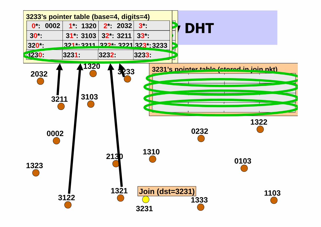
3231’s pointer table (stored in join pkt)1*: 1320 2*: 3*: 0*:

31*: 32*: 33*: 321*: 322*: 3221 323*:

30*: 320*:

3231: 3232: 3233: 3230:

31033211

2130 31223211

32333233

0002

Join (dst=3231)

1321’s pointer table (base=4, digits=4)1*: 1320 2*: 3*: 0*:

11*: 12*: 13*: 131*: 132*: 133*:

10*: 130*:

1321: 1322: 1322 1323: 1320: 1310

2130 31221323 13331323

00021023

3122’s pointer table (base=4, digits=4)1*: 1320 2*: 3*: 0*:

31*: 32*: 33*: 311*: 312*: 313*:

30*: 310*: 3103

3121: 3122: 3123: 3120:

31033211

20323211

00023211’s pointer table (base=4, digits=4)

1*: 1320 2*: 3*: 0*: 31*: 32*: 33*: 321*: 322*: 3221 323*:

30*: 320*:

3211: 3212: 3213: 3210:

31032032

3233

00023233’s pointer table (base=4, digits=4)

1*: 1320 2*: 3*: 0*: 31*: 32*: 33*: 321*: 322*: 3221 323*:

30*: 320*:

3231: 3232: 3233: 3230:

31033211

20323211

3233

0002

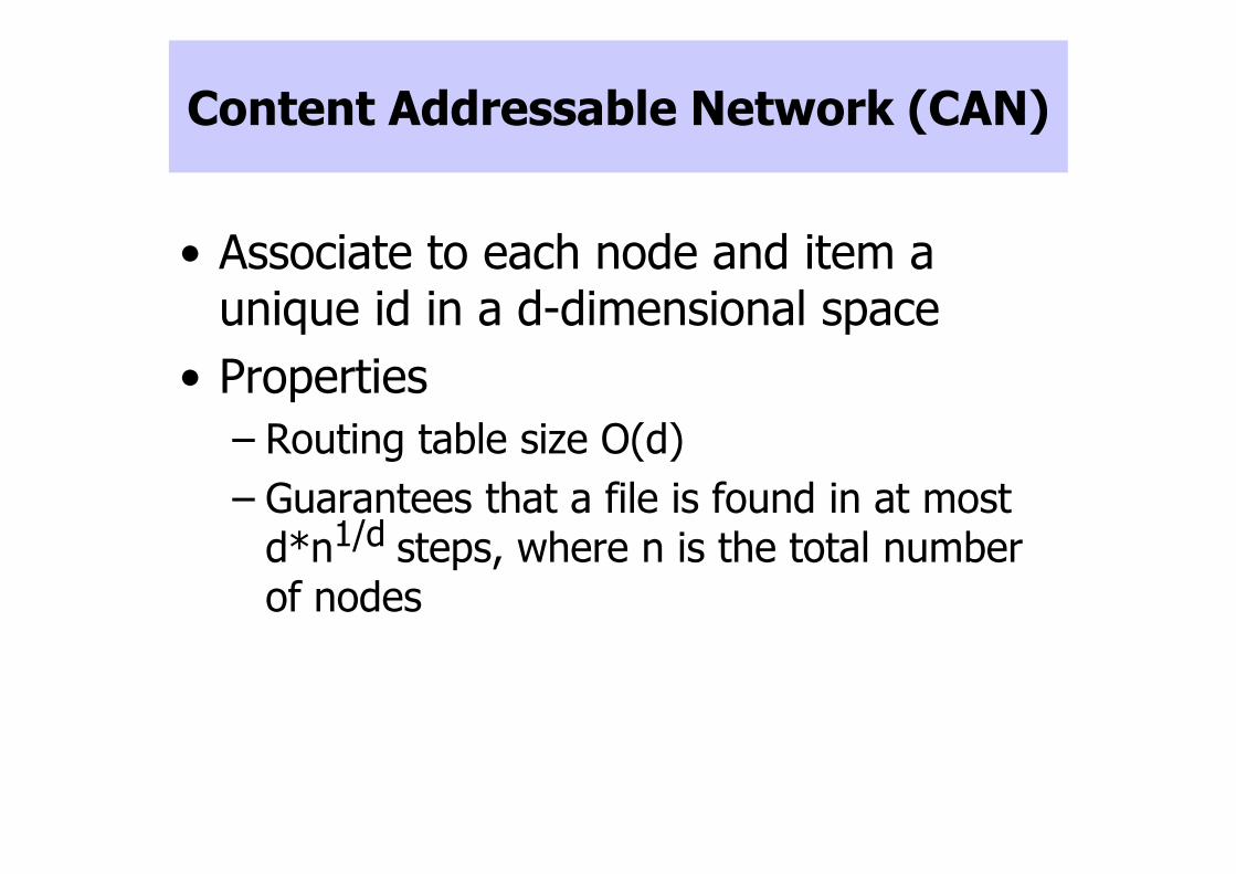
Content Addressable Network (CAN)

• Associate to each node and item a unique id in a d-dimensional space

• Properties

– Routing table size O(d)

– Guarantees that a file is found in at most d*n1/d steps, where n is the total number of nodes

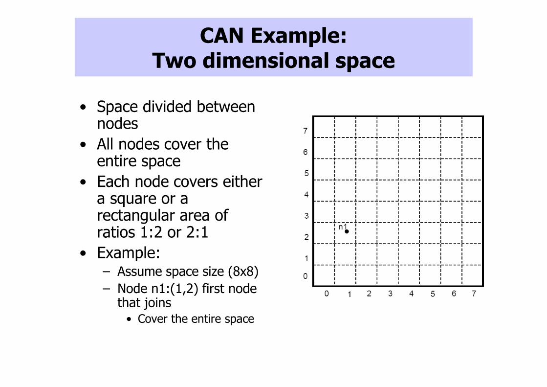
CAN Example: Two dimensional space

• Space divided between nodes

• All nodes cover the entire space

• Each node covers either a square or a rectangular area of ratios 1:2 or 2:1

• Example:– Assume space size (8x8)

– Node n1:(1,2) first node that joins

• Cover the entire space

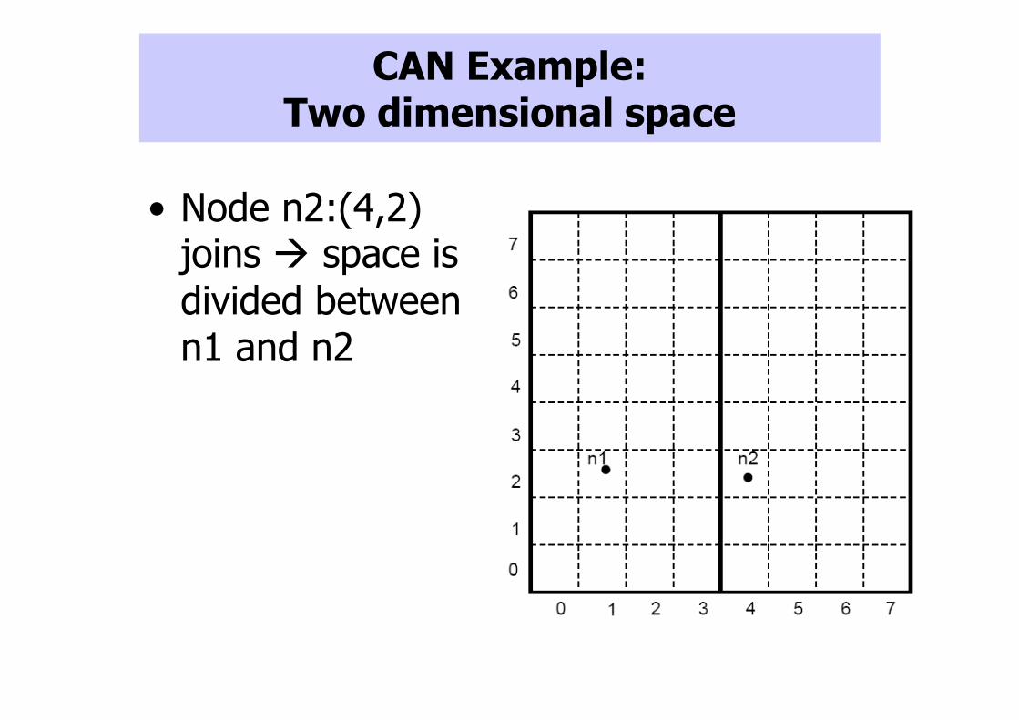
CAN Example: Two dimensional space

• Node n2:(4,2) joins � space is

divided between n1 and n2

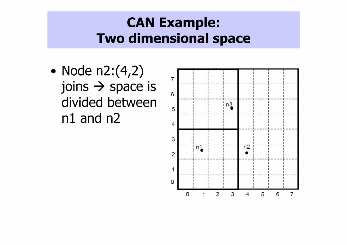
CAN Example: Two dimensional space

• Node n2:(4,2) joins � space is

divided between n1 and n2

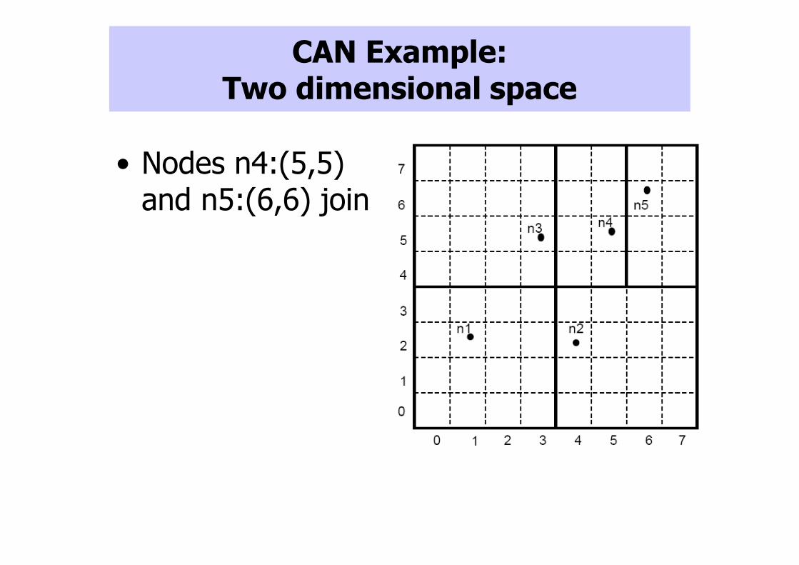
CAN Example: Two dimensional space

• Nodes n4:(5,5) and n5:(6,6) join

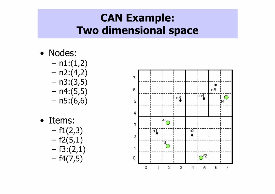
CAN Example: Two dimensional space

• Nodes: – n1:(1,2)– n2:(4,2)– n3:(3,5)– n4:(5,5)– n5:(6,6)

• Items:– f1(2,3)– f2(5,1)– f3:(2,1)– f4(7,5)

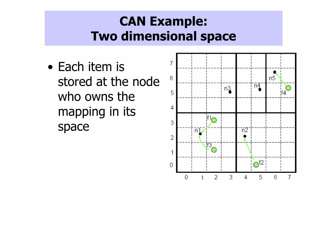
CAN Example: Two dimensional space

• Each item is stored at the node who owns the mapping in its space

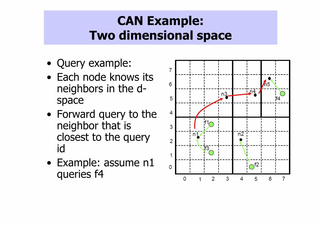
CAN Example: Two dimensional space

• Query example:

• Each node knows its neighbors in the d-space

• Forward query to the neighbor that is closest to the query id

• Example: assume n1 queries f4

Preserving consistency

• What if a node fails?

– Solution: probe neighbors to make sure alive, proactively replicate objects

• What if node joins in wrong position?

– Solution: nodes check to make sure they are in the right order

– Two flavors: weak stabilization, and strong stabilization

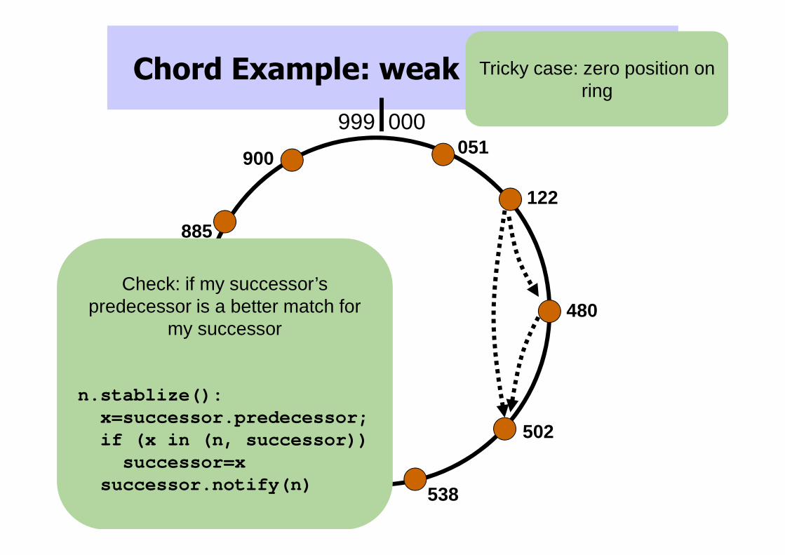
Chord Example: weak stabilization

000999

732

885

900051

122

480

502

538619

670

Check: if my successor’s predecessor is a better match for

my successor

n.stablize():x=successor.predecessor;if (x in (n, successor))successor=x

successor.notify(n)

Tricky case: zero position on ring

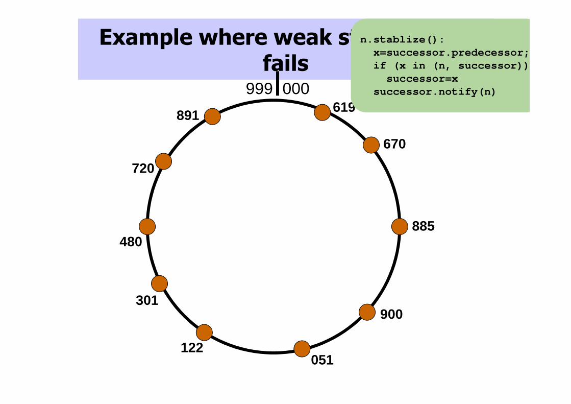
Example where weak stabilization fails

000999

480

720

891619

670

885

900

051122

301

n.stablize():x=successor.predecessor;if (x in (n, successor))

successor=xsuccessor.notify(n)

Comparison of DHT geometries

Geometry Algorithm

Ring Chord

Hypercube CAN

Tree Plaxton

Hybrid =Tree + Ring

Tapestry, Pastry

XORd(id1, id2) = id1 XOR id2

Kademlia

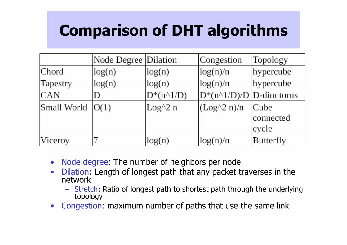
Comparison of DHT algorithms

• Node degree: The number of neighbors per node• Dilation: Length of longest path that any packet traverses in the

network– Stretch: Ratio of longest path to shortest path through the underlying

topology

• Congestion: maximum number of paths that use the same link

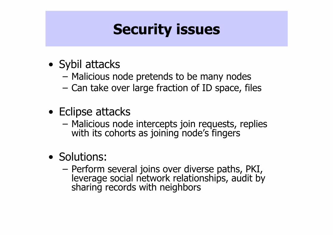
Security issues

• Sybil attacks– Malicious node pretends to be many nodes– Can take over large fraction of ID space, files

• Eclipse attacks– Malicious node intercepts join requests, replies

with its cohorts as joining node’s fingers

• Solutions:– Perform several joins over diverse paths, PKI,

leverage social network relationships, audit by sharing records with neighbors

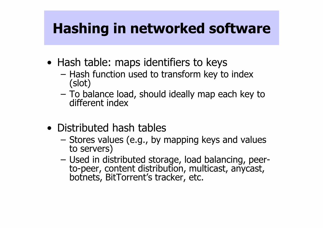
Hashing in networked software

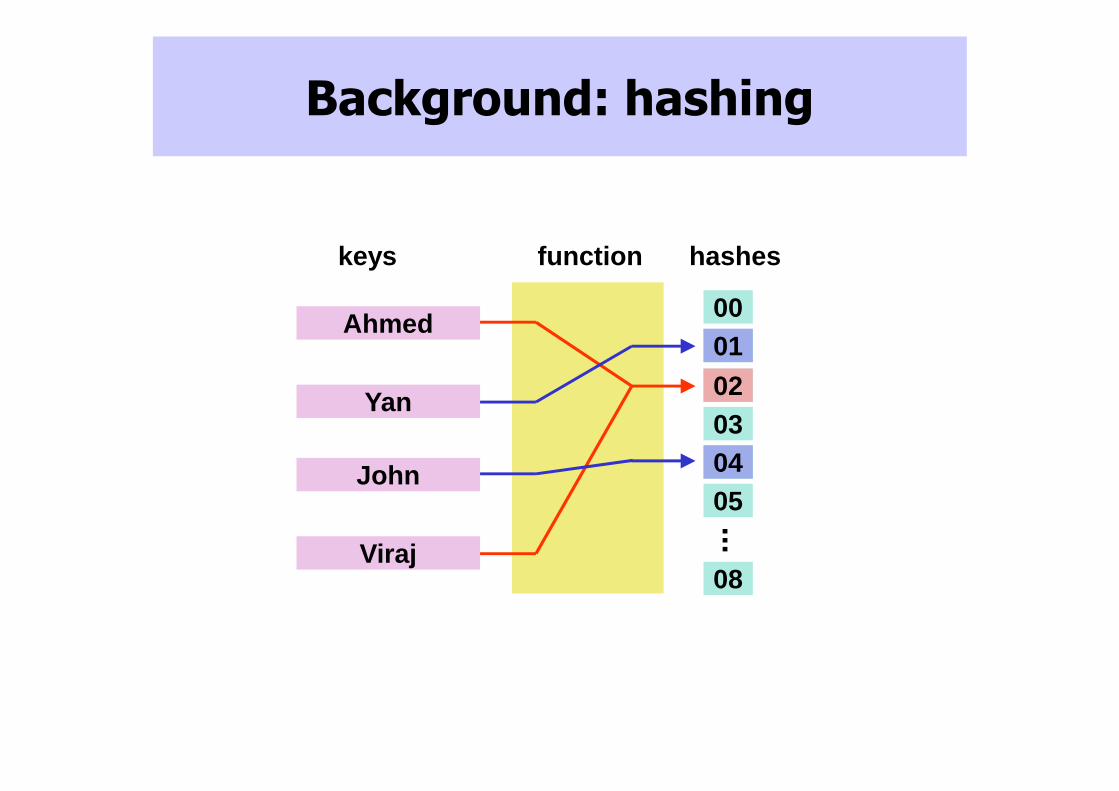
• Hash table: maps identifiers to keys– Hash function used to transform key to index

(slot)– To balance load, should ideally map each key to

different index

• Distributed hash tables– Stores values (e.g., by mapping keys and values

to servers)– Used in distributed storage, load balancing, peer-

to-peer, content distribution, multicast, anycast, botnets, BitTorrent’s tracker, etc.

01

02

04

Background: hashing

00

hashes

03

01

02

0405...

08

function

Ahmed

Yan

John

Viraj

keys

Example

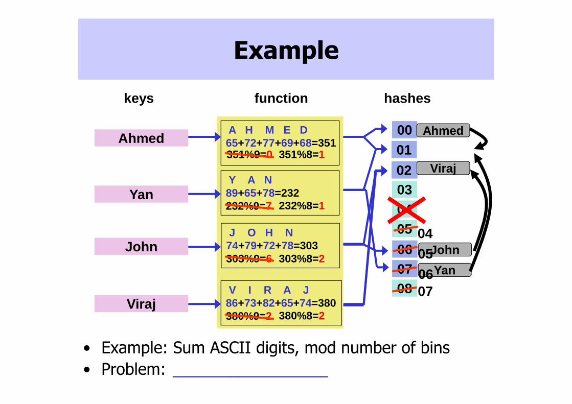
• Example: Sum ASCII digits, mod number of bins

• Problem: failures cause large shifts

00

hashes

01

02030405

function

Yan

John

Ahmed

Viraj

keys

A H M E D

Y A N89+65+78=232232%9=7

J O H N74+79+72+78=303303%9=6

V I R A J86+73+82+65+74=380380%9=2

060708

00

02

0607

65+72+77+69+68=351351%9=0 351%8=1

232%8=1

303%8=2

380%8=2

Ahmed

Yan

John

Viraj

04

05

0607

01

02

___________________

Solution: Consistent Hashing

• Hashing function that reduces churn

• Addition or removal of one slot does not significantly change mapping of keys to slots

• Good consistent hashing schemes change mapping of K/N entries on single slot addition

– K: number of keys

– N: number of slots

• E.g., map keys and slots to positions on circle

– Assign keys to closest slot on circle

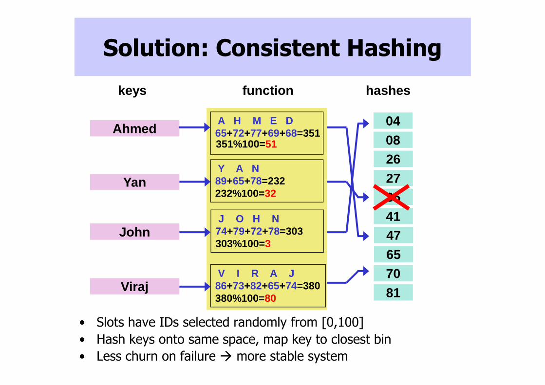
Solution: Consistent Hashing

• Slots have IDs selected randomly from [0,100]

• Hash keys onto same space, map key to closest bin

• Less churn on failure � more stable system

hashesfunction

Yan

John

Ahmed

Viraj

keys

Y A N89+65+78=232232%100=32

J O H N74+79+72+78=303303%100=3

V I R A J86+73+82+65+74=380380%100=80

A H M E D65+72+77+69+68=351351%100=51

04082627354147657081

Network layer DHTs

44

Postal Service

Scenario: Sending a Letter

3400 Walnut St. Philadelphia, PA 19104

Address:

450 Lancaster Ave. 3400 Walnut St.

900 Spruce St.

Name: B

A B

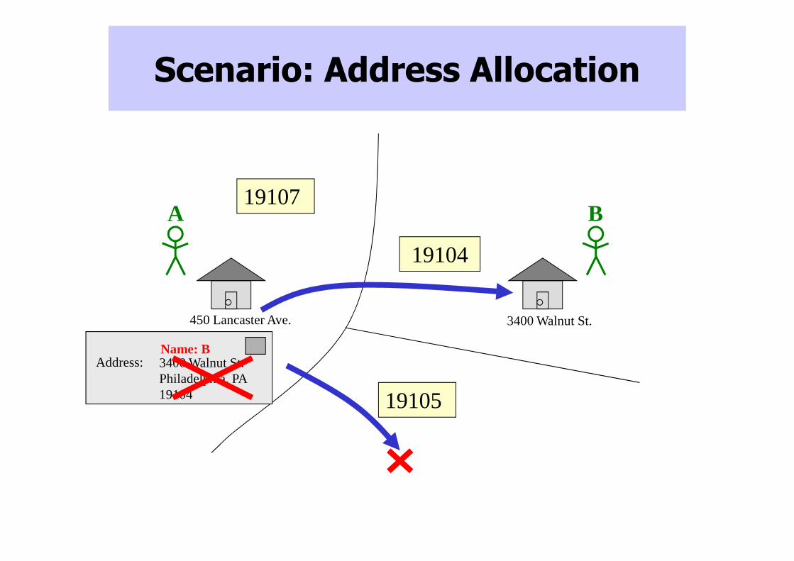
Scenario: Address Allocation

450 Lancaster Ave. 3400 Walnut St.

19104

19105

19107A B

3400 Walnut St. Philadelphia, PA19104

Address:Name: B

Postal Service

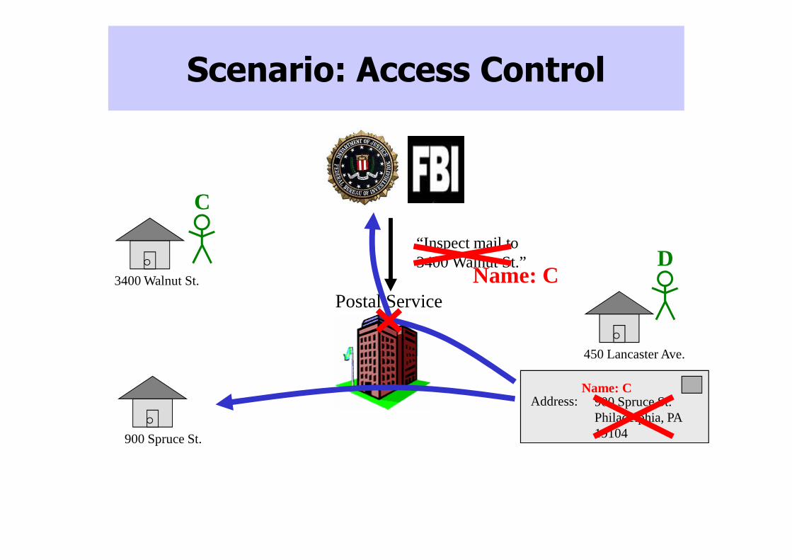
Scenario: Access Control

3400 Walnut St.

900 Spruce St.

“Inspect mail to 3400 Walnut St.”

450 Lancaster Ave.

C

D

3400 Walnut St. Philadelphia, PA19104

Address: 900 Spruce St. Philadelphia, PA 19104

Address:Name: C

Name: C

How Routing Works Today

• Each node has an identity• Goal: find path to destination

Send(msg,Q)

B

J

S

K

Q

F

V

X

A

Area 1

Area 2

Area 4

Area 3

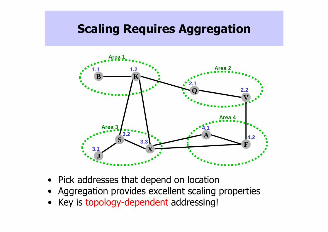
Scaling Requires Aggregation

• Pick addresses that depend on location• Aggregation provides excellent scaling properties• Key is topology-dependent addressing!

B

J

S

K

Q

F

V

X

A

1.1 1.2

2.12.2

4.2

4.1

3.33.2

3.1

Topology-Dependent Addresses Aren’t Always Possible

• Networks can’t use topology-dependent addresses because topology changes so rapidly

• Decades-long search for scalable routing algorithms for ad hoc networks

Topology-Dependent Addresses Aren’t Always Desirable

• Using topology-based addresses in the Internet complicates access controls, mobility, and multihoming

• Would like to embed persistent identities into network-layer addresses

Can We Scale without Topology-Dependent Addresses?

• Is it possible to scale without aggregation?

• Distributed Hash Tables don’t solve this problem

This Talk

• Will describe how to route scalably on flat identifiers that applies to both:

• Wireless networks:

– Challenge is dynamics

• Wired networks:

– Challenge is scale, policies, and dynamics

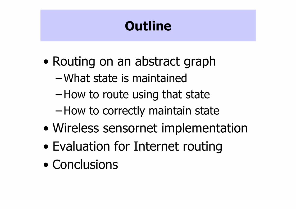
Outline

• Routing on an abstract graph

– What state is maintained

– How to route using that state

– How to correctly maintain state

• Wireless sensornet implementation

• Evaluation for Internet routing

• Conclusions

J

K Q

F

V

A

S

Network topology

X

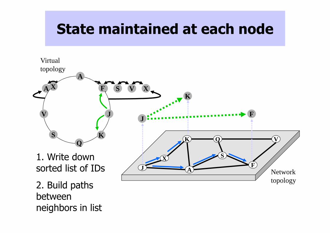
State maintained at each node

A F J K Q S V X

J

K

F

1. Write down sorted list of IDs

2. Build paths between neighbors in list

Virtual topology

F

A

J

KQ

V

S

X

J

K Q

F

V

A

S

Network topology

X

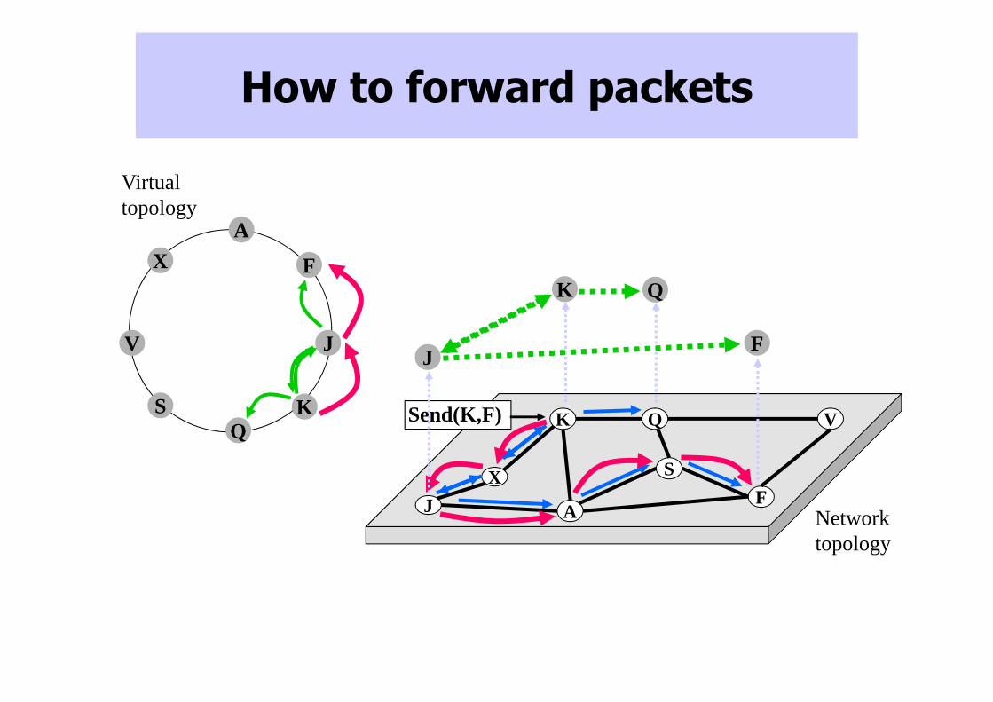
How to forward packets

Virtual topology

F

A

J

KQ

V

S

X

Send(K,F)

Q

J

K

F

J

K Q

F

V

A

S

Network topology

X

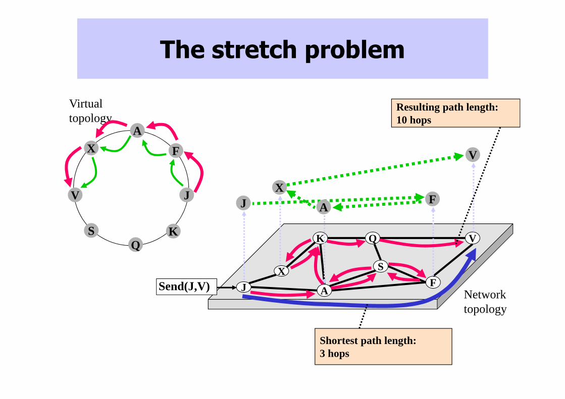
The stretch problem

Virtual topology

F

A

J

KQ

V

S

X

Send(J,V)

J FA

X

V

Resulting path length: 10 hops

Shortest path length: 3 hops

J

K Q

F

V

A

S

Network topology

X

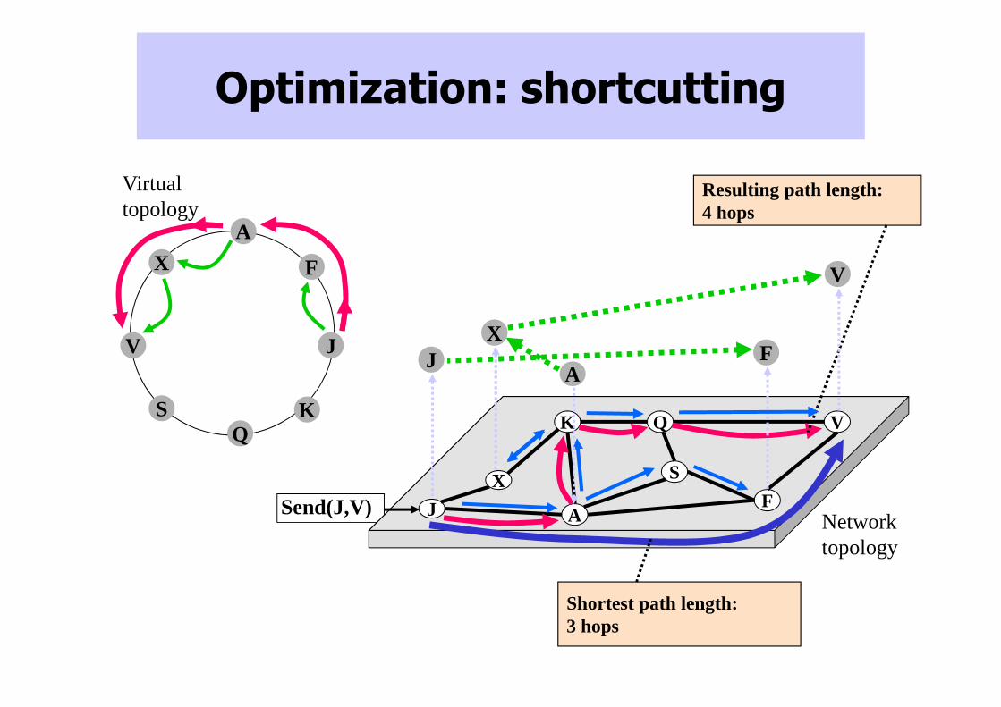
Optimization: shortcutting

Virtual topology

F

A

J

KQ

V

S

X

Send(J,V)

Resulting path length: 4 hops

Shortest path length: 3 hops

J FX

V

A

X

A summary so far…

• The algorithm has two parts

– Route linearly around the ring

– Shortcut when possible

• Up next, the technical details…

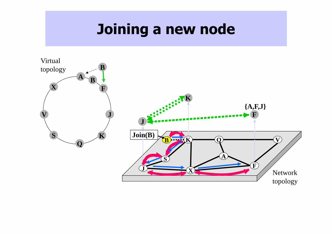
Joining a new node

J

K Q

F

V

X

A

B

Network topology

S

B

K

JF

Join(B)

F

A

J

KQ

V

S

X

Virtual topology

{A,F,J}

B

How to maintain state

J

K Q

F

V

X

A

Network topology

S

JF

F

A

J

KQ

V

S

X

Virtual topology Goal #2:

Ensure each pointer path points to correct global successor/predecessor

Goal #1:Ensure each pointer path is properly maintained

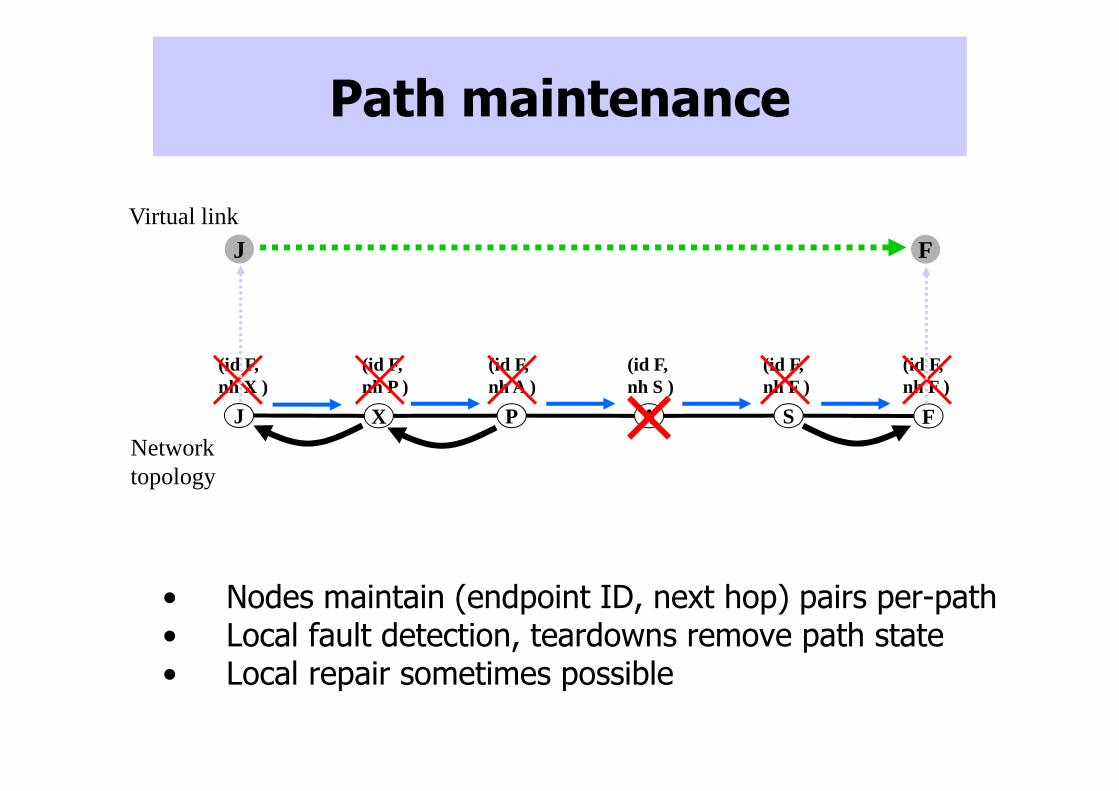
Path maintenance

• Nodes maintain (endpoint ID, next hop) pairs per-path• Local fault detection, teardowns remove path state• Local repair sometimes possible

J PX SA F

(id F,nh X )

(id F,nh P )

(id F,nh A )

(id F,nh S )

(id F,nh F )

(id F,nh F )

J FVirtual link

Network topology

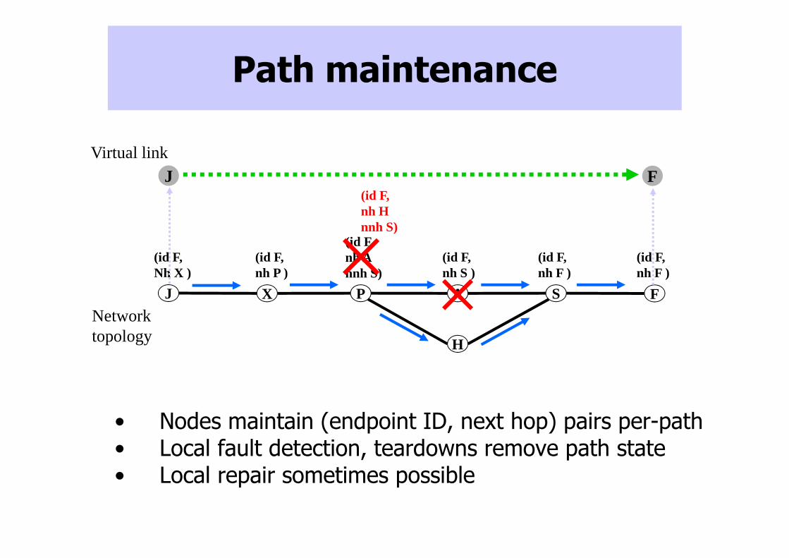
Path maintenance

• Nodes maintain (endpoint ID, next hop) pairs per-path• Local fault detection, teardowns remove path state• Local repair sometimes possible

J PX SA F

(id F,Nh X )

(id F,nh P )

(id F,nh Annh S)

(id F,nh S )

(id F,nh F )

(id F,nh F )

H

(id F,nh Hnnh S)

J FVirtual link

Network topology

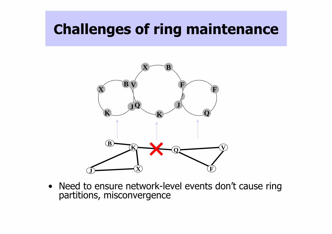
Challenges of ring maintenance

• Need to ensure network-level events don’t cause ring partitions, misconvergence

J

K Q

F

V

X

B

F

Q

V

B

K

X

J J

F

KQ

V

X B

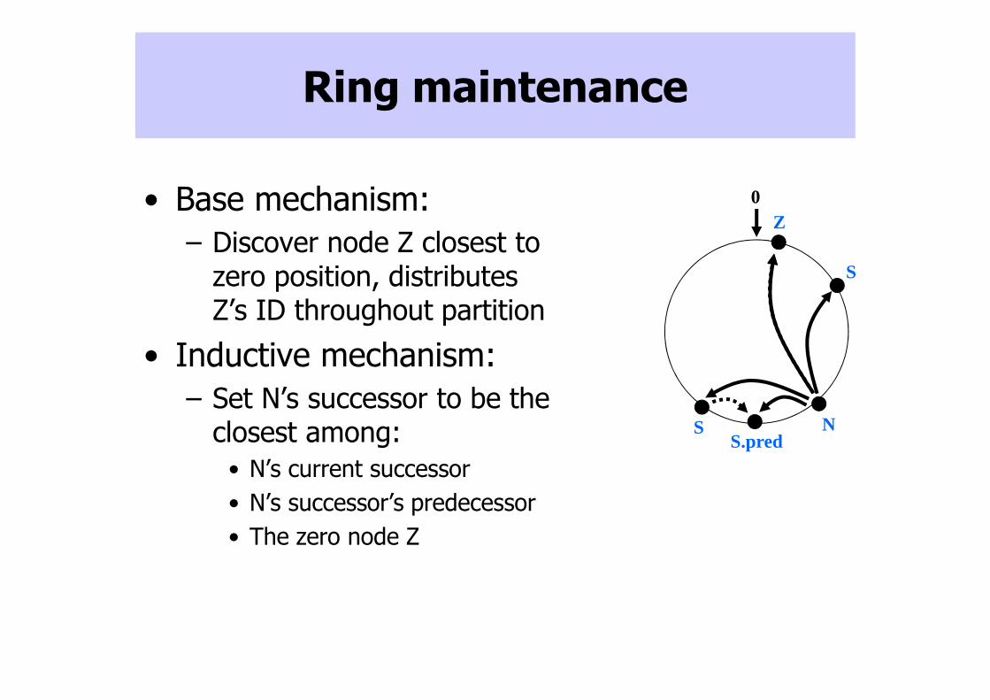
Ring maintenance

• Base mechanism:

– Discover node Z closest to zero position, distributes Z’s ID throughout partition

• Inductive mechanism:

– Set N’s successor to be the closest among:

• N’s current successor

• N’s successor’s predecessor

• The zero node Z

Z0

NSS.pred

S

[1…k-2]

[k+1…0]

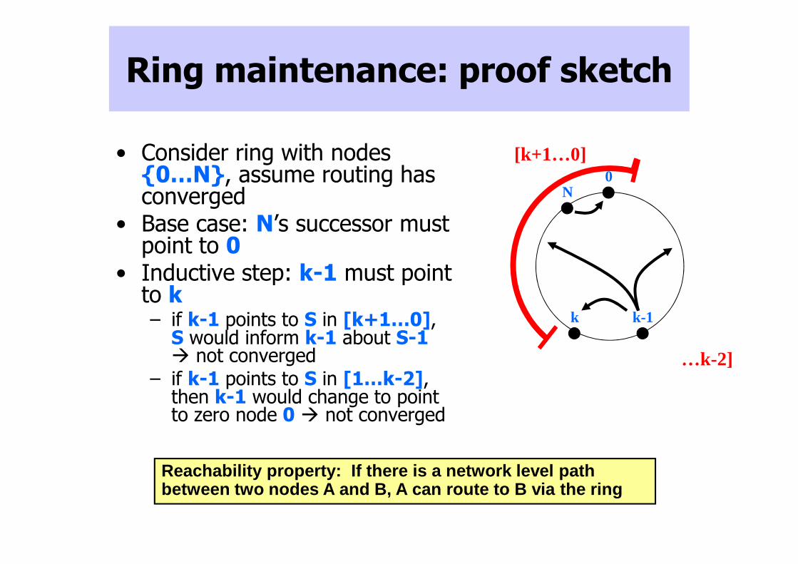
Ring maintenance: proof sketch

• Consider ring with nodes {0…N}, assume routing has converged

• Base case: N’s successor must point to 0

• Inductive step: k-1 must point to k– if k-1 points to S in [k+1…0],

S would inform k-1 about S-1� not converged

– if k-1 points to S in [1…k-2], then k-1 would change to point to zero node 0 � not converged

0N

k k-1

Reachability property: If there is a network level path between two nodes A and B, A can route to B via the ring

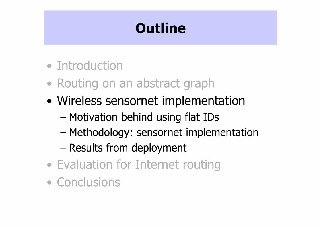
Outline

• Introduction

• Routing on an abstract graph

• Wireless sensornet implementation

– Motivation behind using flat IDs

– Methodology: sensornet implementation

– Results from deployment

• Evaluation for Internet routing

• Conclusions

Why flat IDs for wireless?

• Multihop wireless networks on the horizon

– Rooftop networks, sensornets, ad-hoc networks

• Flat IDs scale in dynamic networks

– No location service needed

– Flood-free maintenance reduces state, control traffic

• Developed and deployed prototype implementation for wireless sensornets

– Extensions: failure detection, link-estimation

Methodology

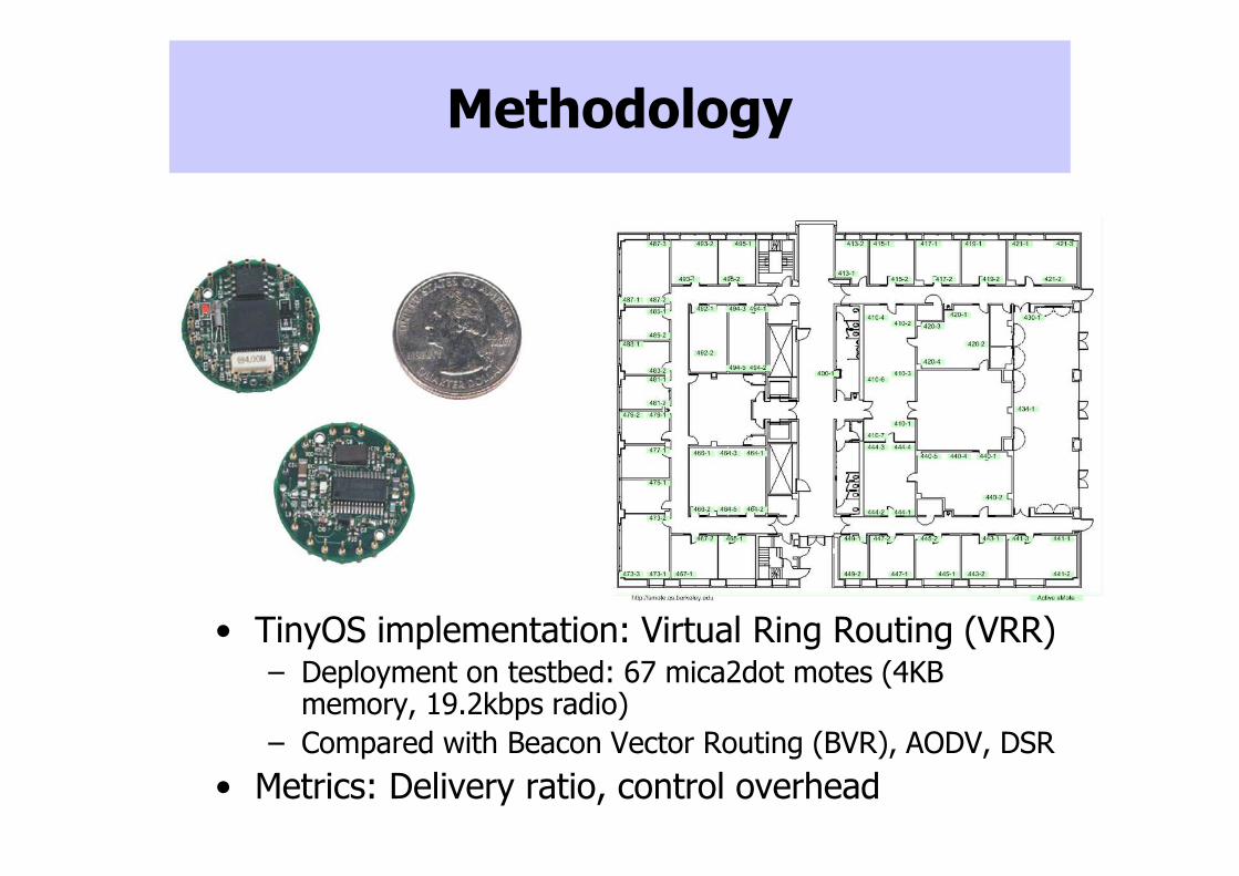
• TinyOS implementation: Virtual Ring Routing (VRR)– Deployment on testbed: 67 mica2dot motes (4KB

memory, 19.2kbps radio)

– Compared with Beacon Vector Routing (BVR), AODV, DSR

• Metrics: Delivery ratio, control overhead

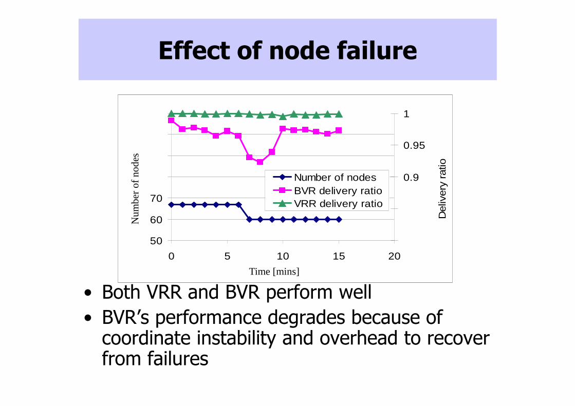
Effect of node failure

• Both VRR and BVR perform well

• BVR’s performance degrades because of coordinate instability and overhead to recover from failures

50

60

70

80

90

100

110

0 5 10 15 20

Time (mins)

Num

ber

of n

odes

0.8

0.85

0.9

0.95

1

Del

iver

y ra

tio

Number of nodesBVR delivery ratioVRR delivery ratio

Time [mins]

Nu

mb

er o

f no

des

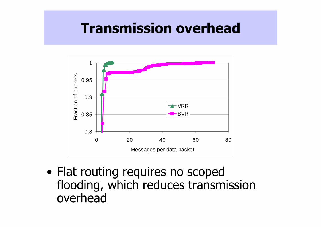
Transmission overhead

• Flat routing requires no scoped flooding, which reduces transmission overhead

Time [mins]

Nu

mb

er o

f no

des

0.8

0.85

0.9

0.95

1

0 20 40 60 80

Messages per data packet

Fra

ctio

n of

pac

kets

VRRBVR

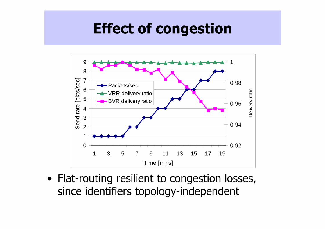
Effect of congestion

• Flat-routing resilient to congestion losses, since identifiers topology-independent

0

1

2

3

4

5

6

7

8

9

1 3 5 7 9 11 13 15 17 19

Time [mins]

Sen

d ra

te [

pkts

/sec

]

0.92

0.94

0.96

0.98

1

Del

iver

y ra

tio

Packets/secVRR delivery ratioBVR delivery ratio

Outline

• Introduction

• Routing on an abstract graph

• Wireless sensornet implementation

• Evaluation for Internet routing

– Motivation behind using flat IDs

– Extensions to support policies, improve scaling

– Performance evaluation on Internet-size graphs

• Conclusions

Why flat IDs for the Internet?

• Today’s Internet conflates addressing with identity

• Flat IDs sidestep this problem completely

– Provides network routing without any mention of location

– Benefits: no need for name resolution service, simpler configuration, simpler access controls

Challenges of Internet routing

• Internet routing is very different from wireless routing

– Challenges: policies, scaling

• Need new mechanisms to deal with these challenges

– Policy-safe successor paths

– Locality-based pointer caching

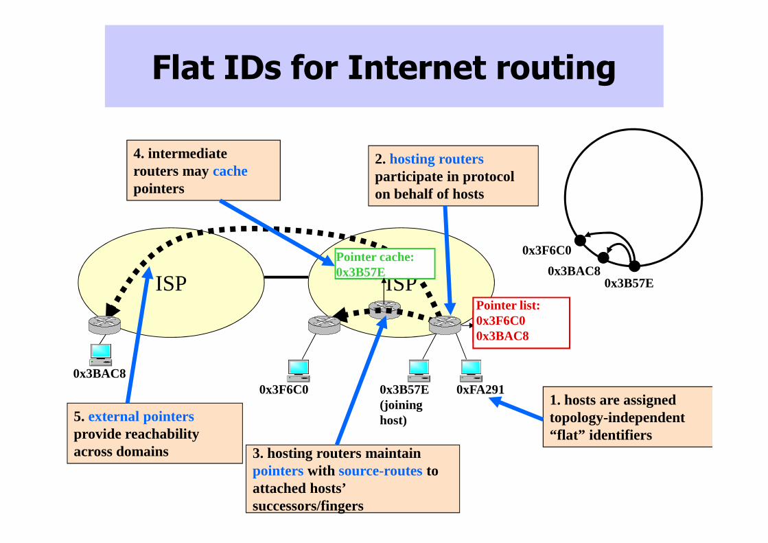
Flat IDs for Internet routing

ISPISP

0xFA2910x3B57E(joining host)

0x3F6C0

0x3BAC80x3B57E

0x3F6C0

Successor list: 0x3F6C0

Pointer list: 0x3F6C00x3BAC8

Pointer cache: 0x3B57E

2. hosting routersparticipate in protocol on behalf of hosts

3. hosting routers maintain pointers with source-routesto attached hosts’ successors/fingers

4. intermediate routers may cache pointers

5. external pointersprovide reachability across domains

1. hosts are assigned topology-independent “flat” identifiers

0x3BAC8

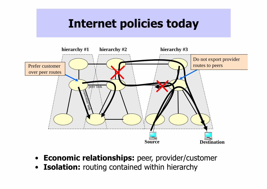
• Economic relationships: peer, provider/customer• Isolation: routing contained within hierarchy

hierarchy #1 hierarchy #2 hierarchy #3

peer link

Internet policies today

• Economic relationships: peer, provider/customer• Isolation: routing contained within hierarchy

Prefer customer over peer routes

Do not export providerroutes to peers

Source Destination

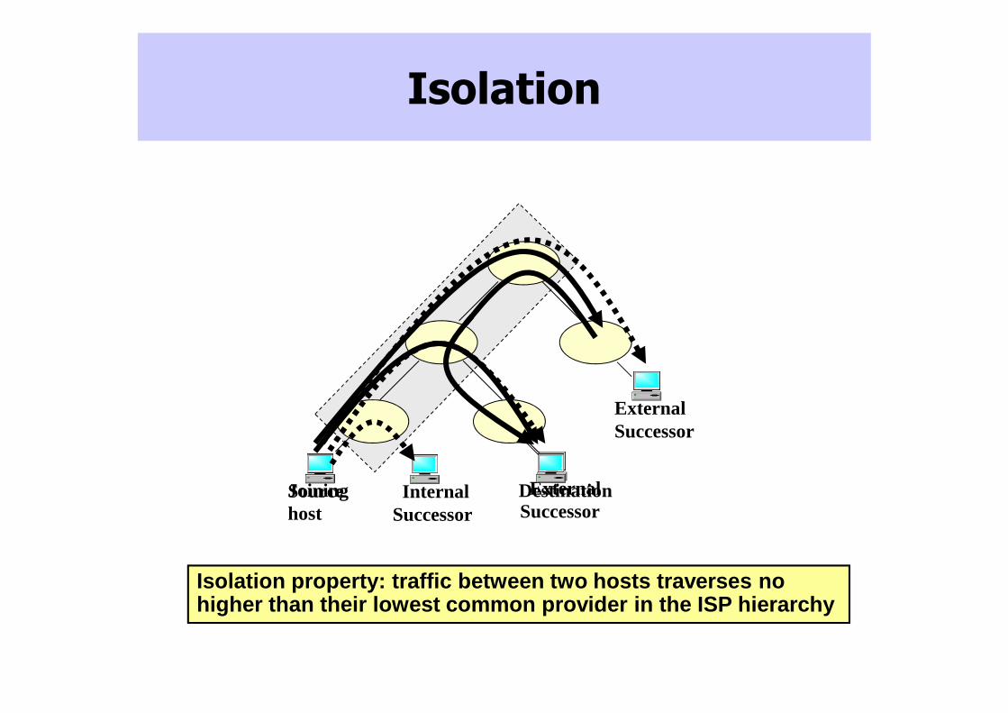
Isolation

Isolation property: traffic between two hosts trave rses no higher than their lowest common provider in the ISP hierarchy

Joininghost

InternalSuccessor

ExternalSuccessor

ExternalSuccessor

Source Destination

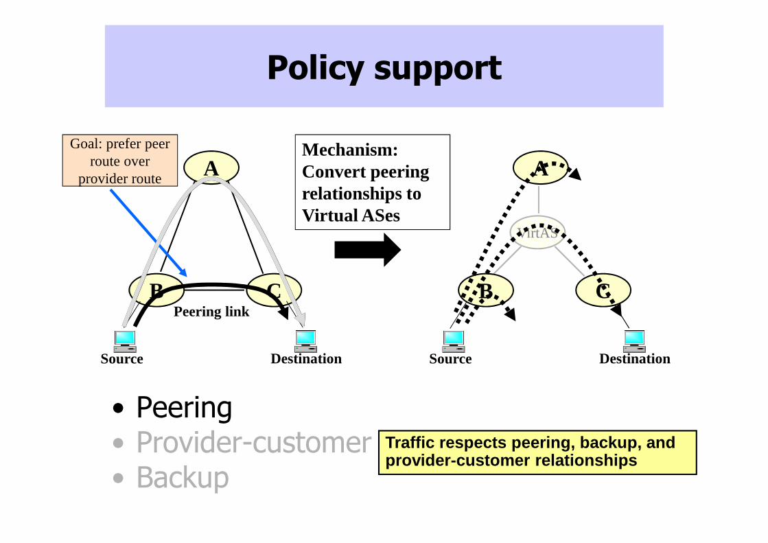
B C

Policy support

Peering link

• Peering• Provider-customer• Backup

Traffic respects peering, backup, and provider-customer relationships

Mechanism:Convert peeringrelationships to Virtual ASes

Source Destination

A

Source Destination

VirtAS

A

CB

Goal: prefer peerroute over

provider route

Evaluation

• Distributed packet-level simulations– Deployed on cluster across 62 machines,

scaled to 300 million hosts– Inferred Internet topology from

Routeviews, Rocketfuel, CAIDA skitter traces

• Implementation– Ran on Planetlab as overlay, covering 82

ASes– Configured inter-ISP policies from

Routeviews traces

• Metrics: stretch, control overhead

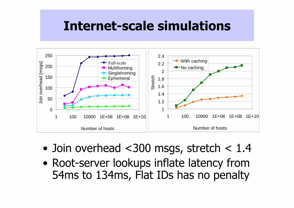
Internet-scale simulations

• Join overhead <300 msgs, stretch < 1.4

• Root-server lookups inflate latency from 54ms to 134ms, Flat IDs has no penalty

1

1.2

1.4

1.6

1.8

2

2.2

2.4

1 100 10000 1E+06 1E+08 1E+10

Number of hosts

Str

etch

With caching

No caching

0

50

100

150

200

250

1 100 10000 1E+06 1E+08 1E+10

Number of hosts

Join

ove

rhea

d [m

sgs] Peering

MultihomingSinglehomingEphemeral

Full-scale