Mauricio Lopes – FNAL

Lecture 5: Stored Energy, Magnetic Forces

and Dynamic Effects

Outlook

2

• Magnetic Forces

• Stored Energy and Inductance

• Fringe Fields

• End Chamfering

• Eddy Currents

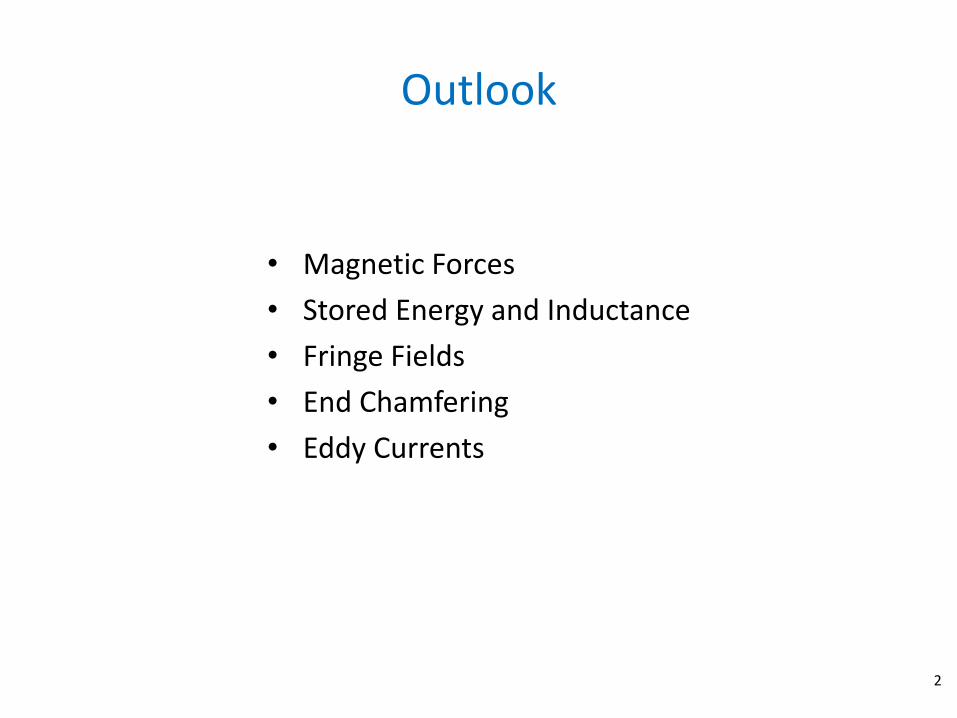
Magnetic Forces

3

• We use the figure to illustrate a simple example.

w a

x

B0

j = uniform current density

F

F

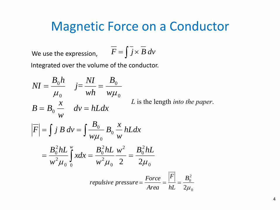
Magnetic Force on a Conductor

4

We use the expression, dvBjF Integrated over the volume of the conductor.

hLdxdvw

xBB

w

B

wh

NIj=

hBNI

0

0

0

0

0

L is the length into the paper.

0

2

02

0

2

2

0

00

2

2

0

0

0

0

22

hLBw

w

hLBxdx

w

hLB

hLdxw

xB

w

BB dvjF

w

0

2

0

2

B

hL

F

Area

Forcepressurerepulsive

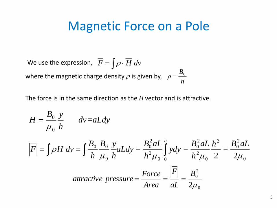
Magnetic Force on a Pole

5

We use the expression, dvHF

h

Bρ 0where the magnetic charge density is given by,

The force is in the same direction as the H vector and is attractive.

dv=aLdyh

yBH

0

0

0

2

0

2

0

2

2

0

00

2

2

0

0

00

2=

2==

aLBh

h

aLBydy

h

aLBaLdy

h

yB

h

BdvHF

h

0

2

0

2

B

aL

F

Area

Forcepressureattractive

Pressure

6

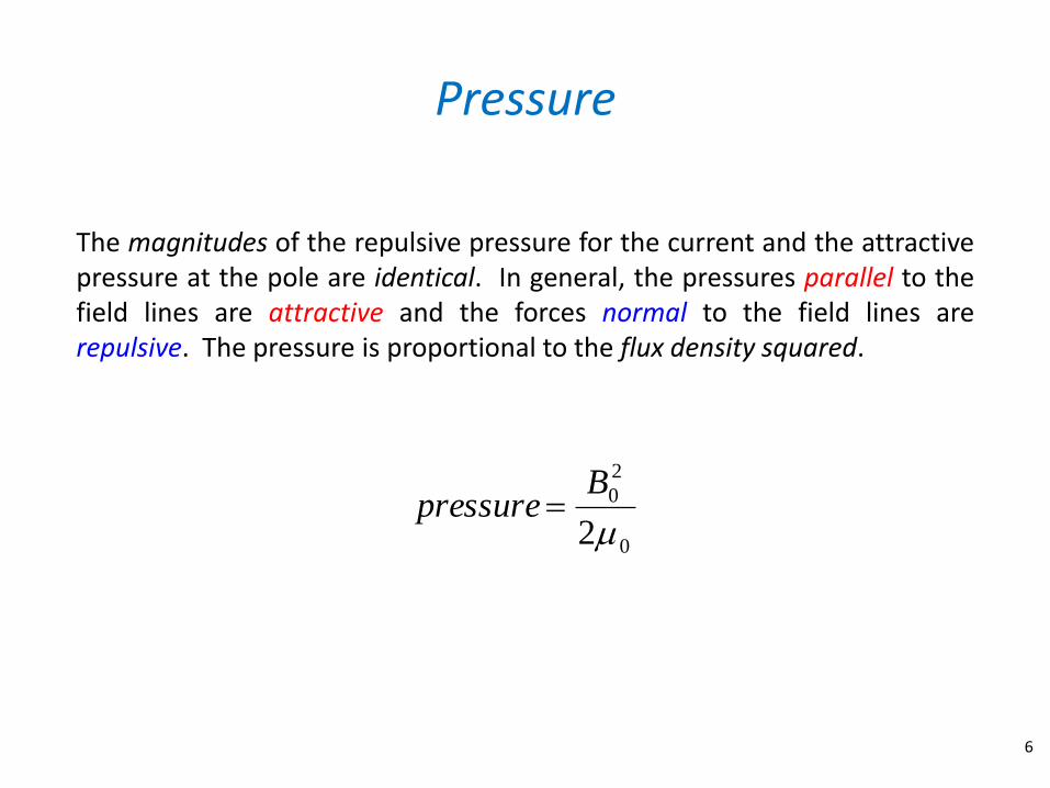
The magnitudes of the repulsive pressure for the current and the attractive pressure at the pole are identical. In general, the pressures parallel to the field lines are attractive and the forces normal to the field lines are repulsive. The pressure is proportional to the flux density squared.

0

2

0

2

Bpressure

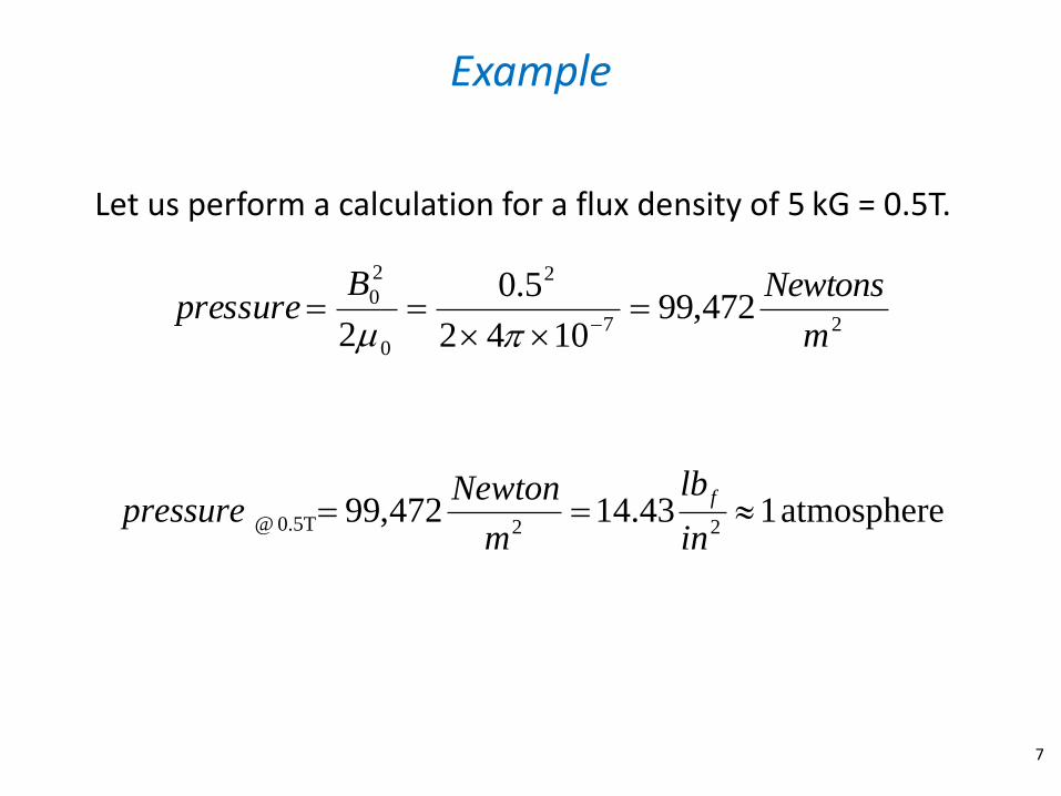
Example

7

Let us perform a calculation for a flux density of 5 kG = 0.5T.

27

2

0

2

0 472,991042

5.0

2 m

NewtonsBpressure

atmosphere 143.14472,99 220.5T @

in

lb

m

Newtonpressure

f

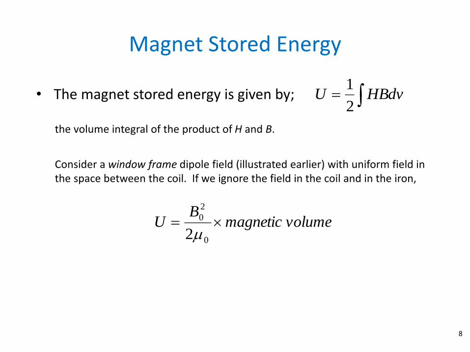
Magnet Stored Energy

8

• The magnet stored energy is given by; HBdvU2

1

the volume integral of the product of H and B.

Consider a window frame dipole field (illustrated earlier) with uniform field in the space between the coil. If we ignore the field in the coil and in the iron,

volumemagneticB

U 2 0

2

0

Magnet Inductance and Ramping Voltage

9

Inductance is given by, 2

2

I

UL

tI

URI

t

I

I

URI

dt

dILRIV

222

In fast ramped magnets, the resistive term is small.

volumeB

tItI

UV

0

2

0

2

22

volume=ahL

N

hBI

0

0

t

NaLBahL

B

tN

hBV

0

0

2

0

0

0

1

Substituting,

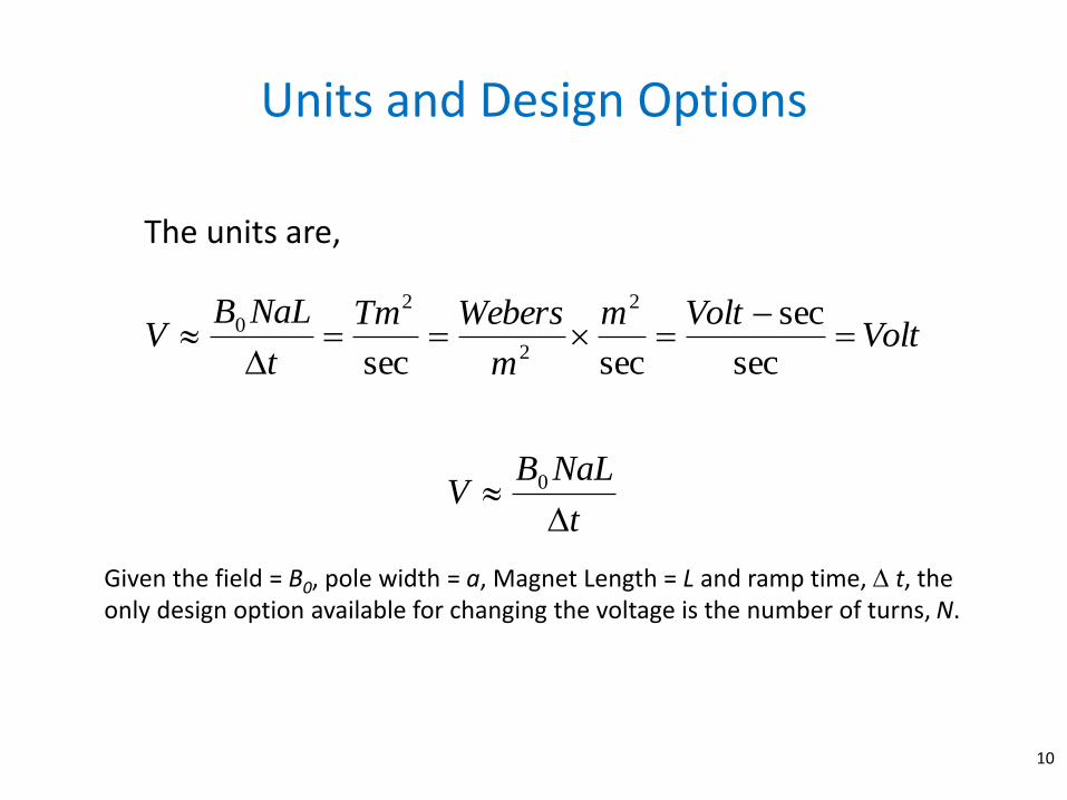
Units and Design Options

10

The units are,

VoltVoltm

m

WebersTm

t

NaLBV

sec

sec

secsec

2

2

2

0

t

NaLBV

0

Given the field = B0, pole width = a, Magnet Length = L and ramp time, t, the only design option available for changing the voltage is the number of turns, N.

Other Magnet Geometries

11

Normally, the stored energy in other magnets (ie. H dipoles, quadrupoles and sextupoles) is not as easily computed. However, for more complex geometries, two dimensional magnetostatic codes will compute the stored energy per unit length of magnet.

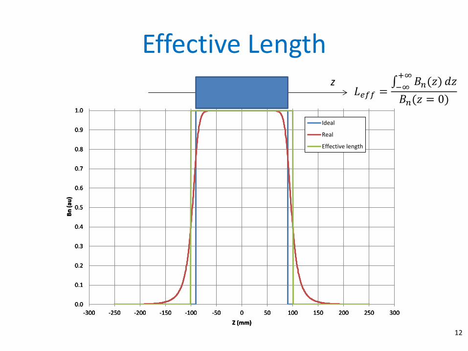
Effective Length

12

0.0

0.1

0.2

0.3

0.4

0.5

0.6

0.7

0.8

0.9

1.0

-300 -250 -200 -150 -100 -50 0 50 100 150 200 250 300

Bn

(au

)

Z (mm)

Ideal

0.0

0.1

0.2

0.3

0.4

0.5

0.6

0.7

0.8

0.9

1.0

-300 -250 -200 -150 -100 -50 0 50 100 150 200 250 300

Bn

(au

)

Z (mm)

Ideal Real

0.0

0.1

0.2

0.3

0.4

0.5

0.6

0.7

0.8

0.9

1.0

-300 -250 -200 -150 -100 -50 0 50 100 150 200 250 300

Bn

(au

)

Z (mm)

Ideal

Real

Effective length

𝐿𝑒𝑓𝑓 = 𝐵𝑛(𝑧)+∞

−∞𝑑𝑧

𝐵𝑛(𝑧 = 0)

z

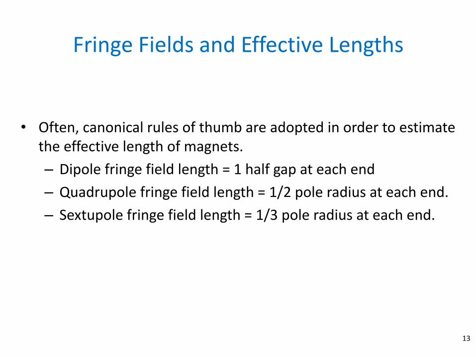
Fringe Fields and Effective Lengths

• Often, canonical rules of thumb are adopted in order to estimate the effective length of magnets.

– Dipole fringe field length = 1 half gap at each end

– Quadrupole fringe field length = 1/2 pole radius at each end.

– Sextupole fringe field length = 1/3 pole radius at each end.

13

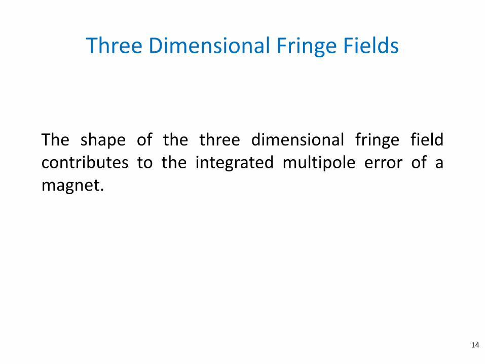
Three Dimensional Fringe Fields

The shape of the three dimensional fringe field contributes to the integrated multipole error of a magnet.

14

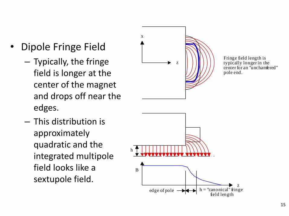
• Dipole Fringe Field

– Typically, the fringe field is longer at the center of the magnet and drops off near the edges.

– This distribution is approximately quadratic and the integrated multipole field looks like a sextupole field.

h

h = "canonical" fringe field length

edge of pole

Fringe field length is typically longer in the center for an "unchamfered" pole end.

z

B

z

x

15

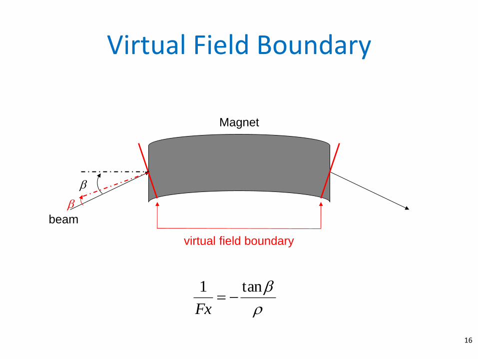
Virtual Field Boundary

16

beam

Magnet

virtual field boundary

tan1

Fx

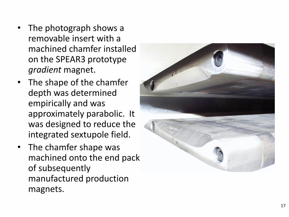
• The photograph shows a removable insert with a machined chamfer installed on the SPEAR3 prototype gradient magnet.

• The shape of the chamfer depth was determined empirically and was approximately parabolic. It was designed to reduce the integrated sextupole field.

• The chamfer shape was machined onto the end packs of subsequently manufactured production magnets.

17

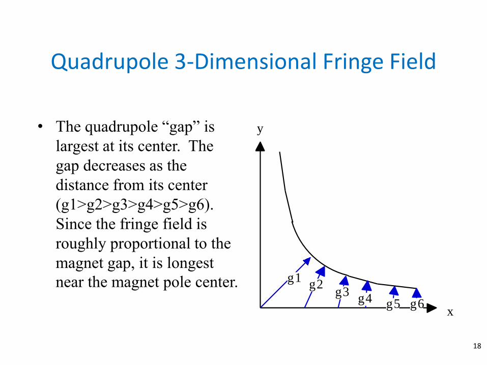
Quadrupole 3-Dimensional Fringe Field

• The quadrupole “gap” is

largest at its center. The

gap decreases as the

distance from its center

(g1>g2>g3>g4>g5>g6).

Since the fringe field is

roughly proportional to the

magnet gap, it is longest

near the magnet pole center. g1g2

g3g4 g5 g6

x

y

18

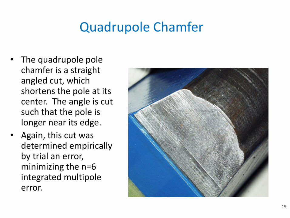
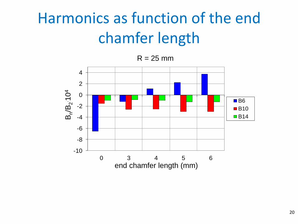
Quadrupole Chamfer

• The quadrupole pole chamfer is a straight angled cut, which shortens the pole at its center. The angle is cut such that the pole is longer near its edge.

• Again, this cut was determined empirically by trial an error, minimizing the n=6 integrated multipole error.

19

-10

-8

-6

-4

-2

0

2

4

0 3 4 5 6

B6

B10

B14

end chamfer length (mm)

R = 25 mm

Bn/B

2. 1

04

Harmonics as function of the end chamfer length

20

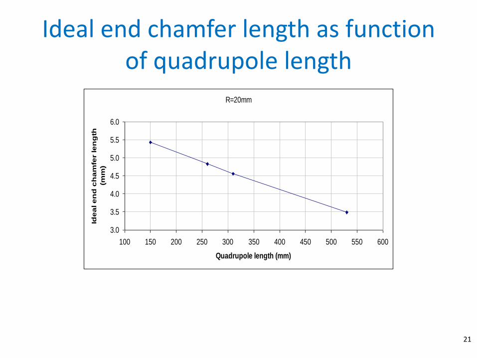
Ideal end chamfer length as function of quadrupole length

21

R=20mm

3.0

3.5

4.0

4.5

5.0

5.5

6.0

100 150 200 250 300 350 400 450 500 550 600

Quadrupole length (mm)

Ide

al e

nd

ch

am

fer le

ng

th

(mm

)

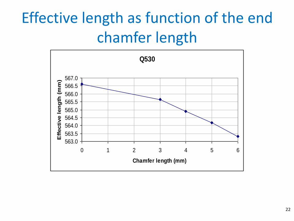
Effective length as function of the end chamfer length

22

Q530

563.0

563.5

564.0

564.5

565.0

565.5

566.0

566.5

567.0

0 1 2 3 4 5 6

Chamfer length (mm)

Eff

ecti

ve l

en

gth

(m

m)

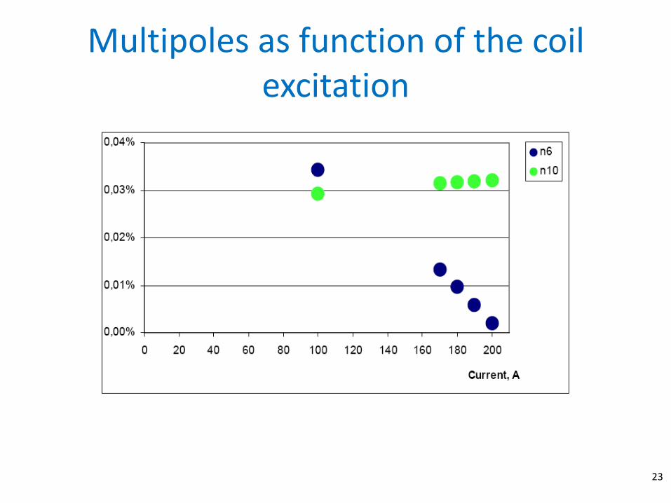
Multipoles as function of the coil excitation

23

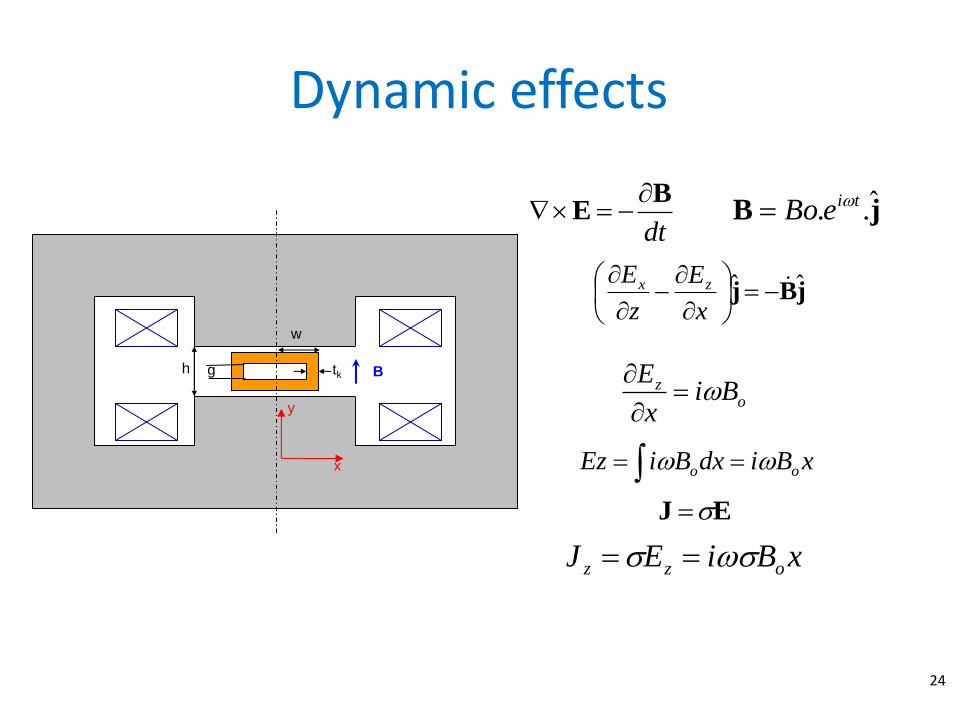
Dynamic effects

24

dt

BE

h

w

g t h

w

g tk B

x

y

jB .̂. tieBo

jBj ˆˆ

x

E

z

E zx

oz Bi

x

E

xBidxBiEz oo EJ

xBiEJ ozz

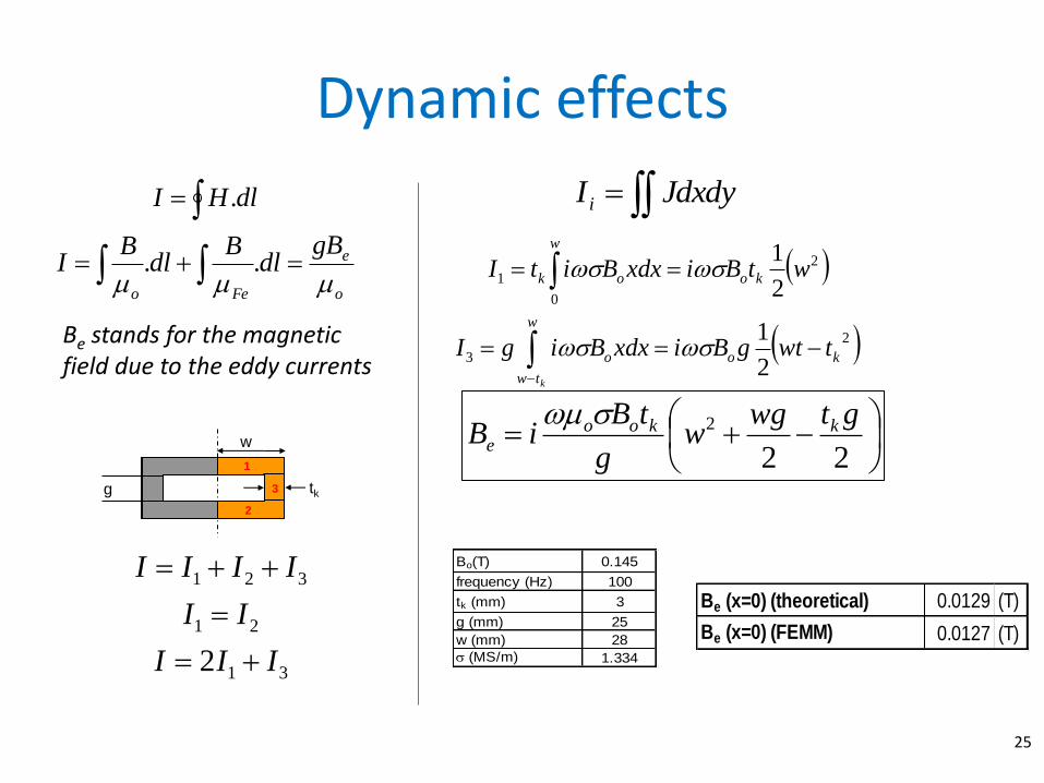
Dynamic effects

25

o

e

Feo

gBdl

Bdl

BI

dlHI

..

.

Be stands for the magnetic field due to the eddy currents

w

1

2

3 g tk

31

21

321

2 III

II

IIII

JdxdyI i

2

0

12

1wtBixdxBitI

w

kook

2

32

1k

w

tw

oo twtgBixdxBigI

k

22

2 gtwgw

g

tBiB kkoo

e

Be (x=0) (theoretical) 0.0129 (T)

Be (x=0) (FEMM) 0.0127 (T)

Bo(T) 0.145

frequency (Hz) 100

tk (mm) 3

g (mm) 25

w (mm) 28

(MS/m) 1.334

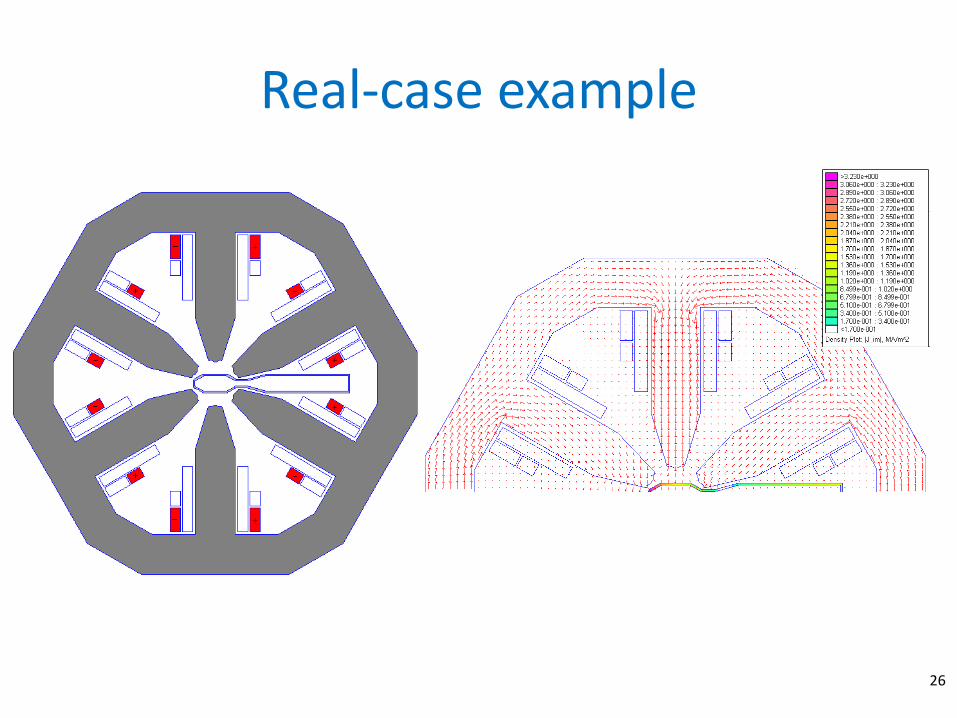
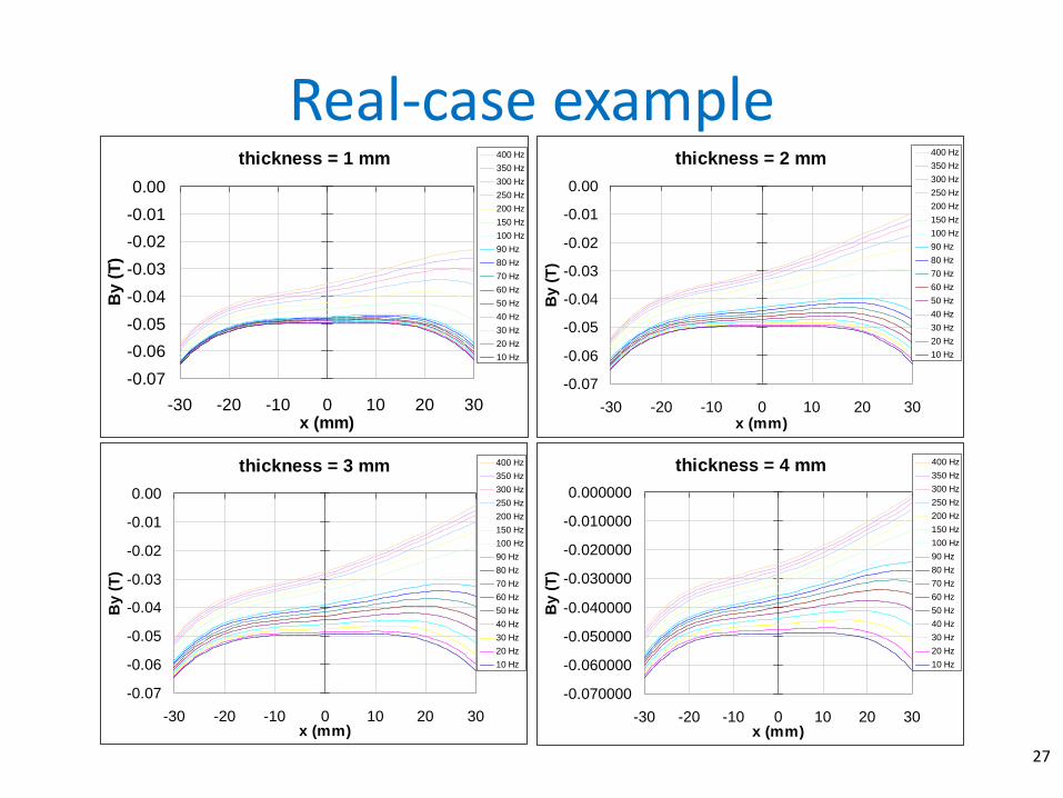
Real-case example

26

Real-case example

27

thickness = 1 mm

-0.07

-0.06

-0.05

-0.04

-0.03

-0.02

-0.01

0.00

-30 -20 -10 0 10 20 30x (mm)

By

(T

)

400 Hz

350 Hz

300 Hz

250 Hz

200 Hz

150 Hz

100 Hz

90 Hz

80 Hz

70 Hz

60 Hz

50 Hz

40 Hz

30 Hz

20 Hz

10 Hz

thickness = 2 mm

-0.07

-0.06

-0.05

-0.04

-0.03

-0.02

-0.01

0.00

-30 -20 -10 0 10 20 30x (mm)

By (

T)

400 Hz

350 Hz

300 Hz

250 Hz

200 Hz

150 Hz

100 Hz

90 Hz

80 Hz

70 Hz

60 Hz

50 Hz

40 Hz

30 Hz

20 Hz

10 Hz

thickness = 3 mm

-0.07

-0.06

-0.05

-0.04

-0.03

-0.02

-0.01

0.00

-30 -20 -10 0 10 20 30x (mm)

By (

T)

400 Hz

350 Hz

300 Hz

250 Hz

200 Hz

150 Hz

100 Hz

90 Hz

80 Hz

70 Hz

60 Hz

50 Hz

40 Hz

30 Hz

20 Hz

10 Hz

thickness = 4 mm

-0.070000

-0.060000

-0.050000

-0.040000

-0.030000

-0.020000

-0.010000

0.000000

-30 -20 -10 0 10 20 30x (mm)

By

(T

)

400 Hz

350 Hz

300 Hz

250 Hz

200 Hz

150 Hz

100 Hz

90 Hz

80 Hz

70 Hz

60 Hz

50 Hz

40 Hz

30 Hz

20 Hz

10 Hz

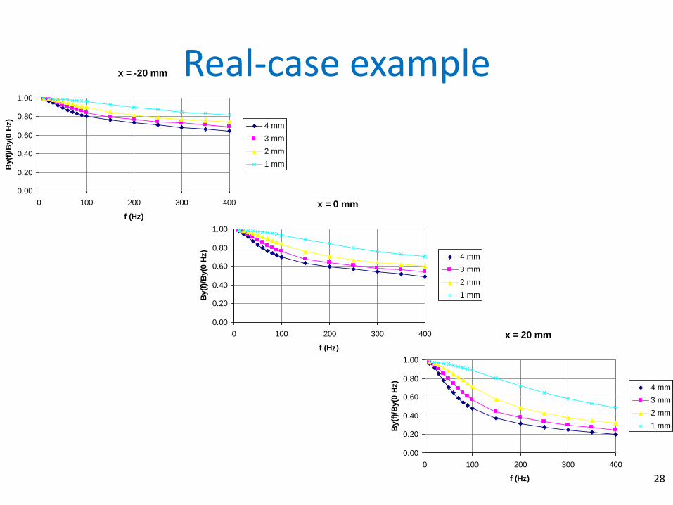
x = 20 mm

0.00

0.20

0.40

0.60

0.80

1.00

0 100 200 300 400

f (Hz)

By(f

)/B

y(0

Hz)

4 mm

3 mm

2 mm

1 mm

28

x = 0 mm

0.00

0.20

0.40

0.60

0.80

1.00

0 100 200 300 400

f (Hz)

By(f

)/B

y(0

Hz)

4 mm

3 mm

2 mm

1 mm

x = -20 mm

0.00

0.20

0.40

0.60

0.80

1.00

0 100 200 300 400

f (Hz)

By(f

)/B

y(0

Hz)

4 mm

3 mm

2 mm

1 mm

Real-case example

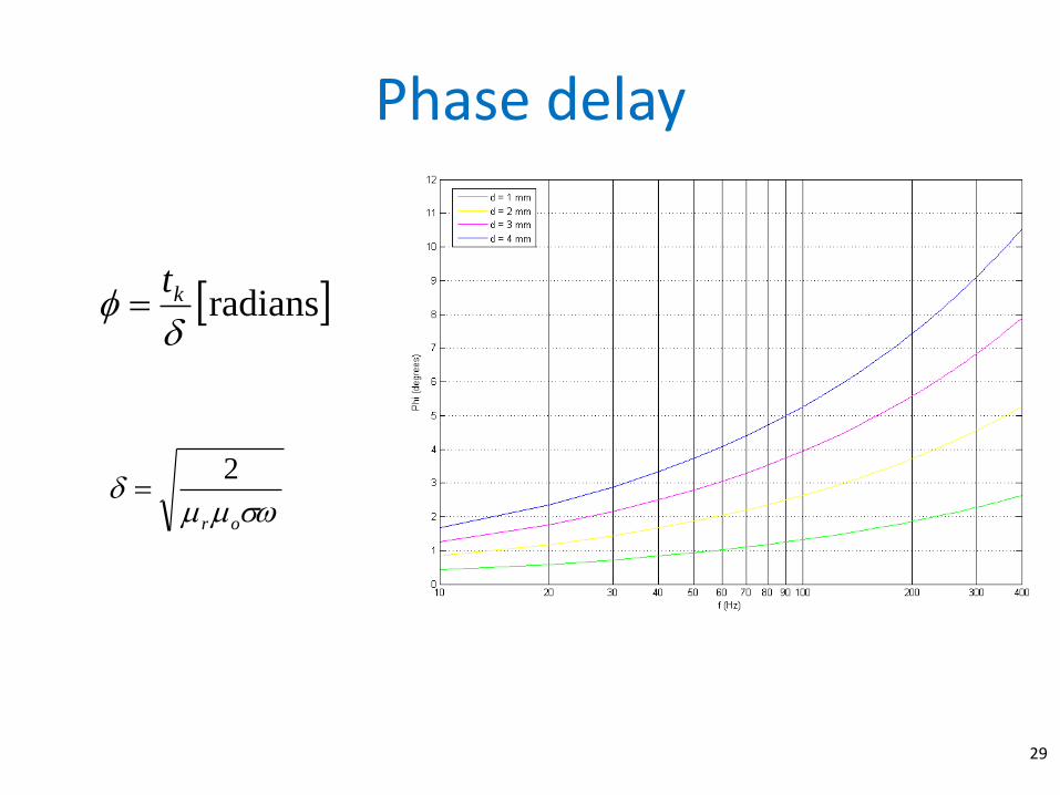
Phase delay

29

or

2

radians

kt

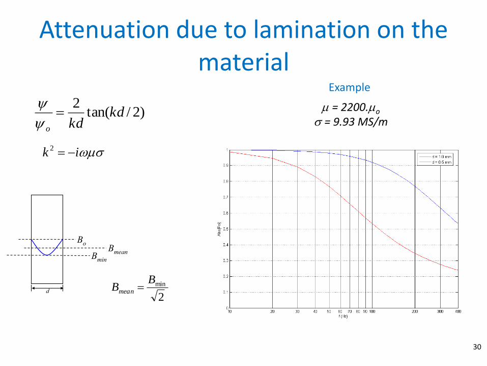
Attenuation due to lamination on the material

30

)2/tan(2

kdkdo

ik 2

= 2200.o

= 9.93 MS/m

Example

Bo

Bmin Bmean

d

2

minBBmean

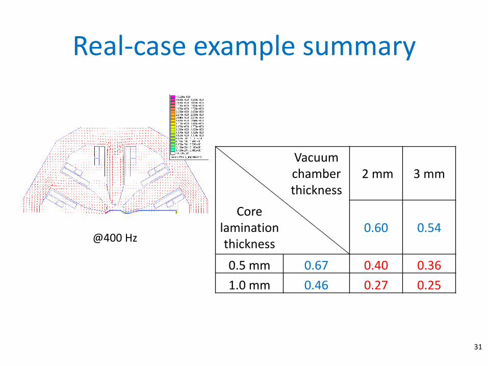
Real-case example summary

31

Vacuum chamber thickness

2 mm 3 mm

Core lamination thickness

0.60 0.54

0.5 mm 0.67 0.40 0.36

1.0 mm 0.46 0.27 0.25

@400 Hz

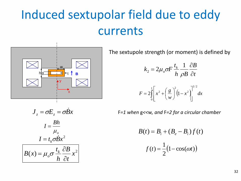
Induced sextupolar field due to eddy currents

32

xBEJ zz

h

w

g t h

w

g t B

x

y

2xBtI ko

BhI

2)( xt

B

h

txB k

o

t

B

Bh

tFk k

o

122

dxxw

gxF

2/11

0

2

2

2 12

F=1 when g<<w, and F=2 for a circular chamber

)()()( tfBBBtB iei

The sextupole strength (or moment) is defined by

)cos(12

1)( ttf

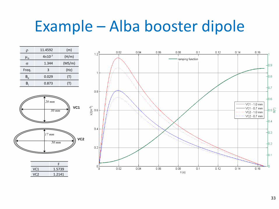
Example – Alba booster dipole

33

11.4592 (m)

o 410-7 (H/m)

1.344 (MS/m)

Freq. 3 (Hz)

Be 0.029 (T)

Bi 0.873 (T)

20 mm

30 mm

17 mm

50 mm

VC1

VC2

F

VC1 1.5739

VC2 1.2141

Summary

34

This chapter showed a collection of “loose-ends” calculations:

• Magnetic Forces • Stored Energy and Inductance • Fringe Fields • End Chamfering • Eddy Currents

Those effects have an impact in the magnet design but also need to be taken into consideration into the magnet fabrication, power supply design, vacuum chamber design and beam optics.

Next…

35

Magnetic measurements