8/16/2017

1

Lecture 31 Slide 1

EE 5337

Computational Electromagnetics (CEM)

Lecture #31

Optimization

These notes may contain copyrighted material obtained under fair use rules.  Distribution of these materials is strictly prohibited  

InstructorDr. Raymond Rumpf(915) 747‐6958rcrumpf@utep.edu

Outline

• Introduction

• The Merit Function

– The “Rectangle” Algorithm

• Direct Methods

– Complete search

– Others

• Stochastic Optimization

– Genetic algorithms

– Simulated annealing

– Particle swarm optimization

Lecture 31 Slide 2

8/16/2017

2

Lecture 31 Slide 3

Introduction

Lecture 31 Slide 4

What is Optimization?

Optimization is simply finding the minimum or a maximum of a function.  In this regard, it is similar to root finding.

Maximum occurs at (2,1)

f(x,y)

The function is usually chosen to be a measure of how “good” something is.

Merit functionFitness functionQuality function

8/16/2017

3

Lecture 31 Slide 5

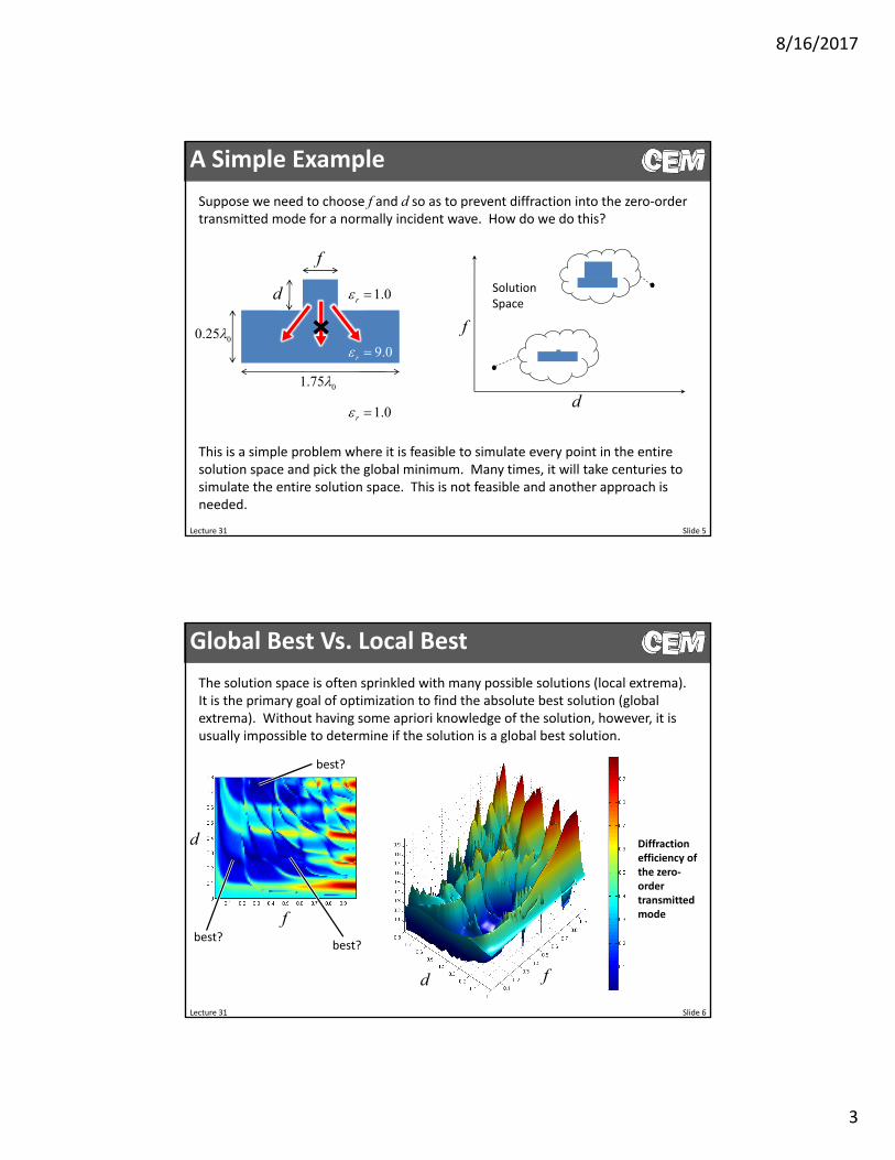
A Simple Example

Suppose we need to choose f and d so as to prevent diffraction into the zero‐order transmitted mode for a normally incident wave.  How do we do this?

d

f

Solution Space

This is a simple problem where it is feasible to simulate every point in the entire solution space and pick the global minimum.  Many times, it will take centuries to simulate the entire solution space.  This is not feasible and another approach is needed.

d

f

9.0r

1.0r

1.0r

00.25

01.75

Lecture 31 Slide 6

Global Best Vs. Local Best

The solution space is often sprinkled with many possible solutions (local extrema).  It is the primary goal of optimization to find the absolute best solution (global extrema).  Without having some apriori knowledge of the solution, however, it is usually impossible to determine if the solution is a global best solution.

d

Diffraction efficiency of the zero‐order transmitted mode

f

d

fbest?

best?

best?

8/16/2017

4

Lecture 31 Slide 7

Common Optimization Algorithms

• Direct Methods

– Complete Search

– Gradient Methods

• Stochastic Optimization

– Particle Swarm Optimization

– Genetic Algorithms

– Simulated Annealing

Only guaranteed method for finding the global extrema.

Converges very quickly to a local extrema.  No global search.

Searches globally.  Usually finds a good solution.  No guarantee it is a global best solution.

Random search to converge to a local best solution.

Lecture 31 Slide 8

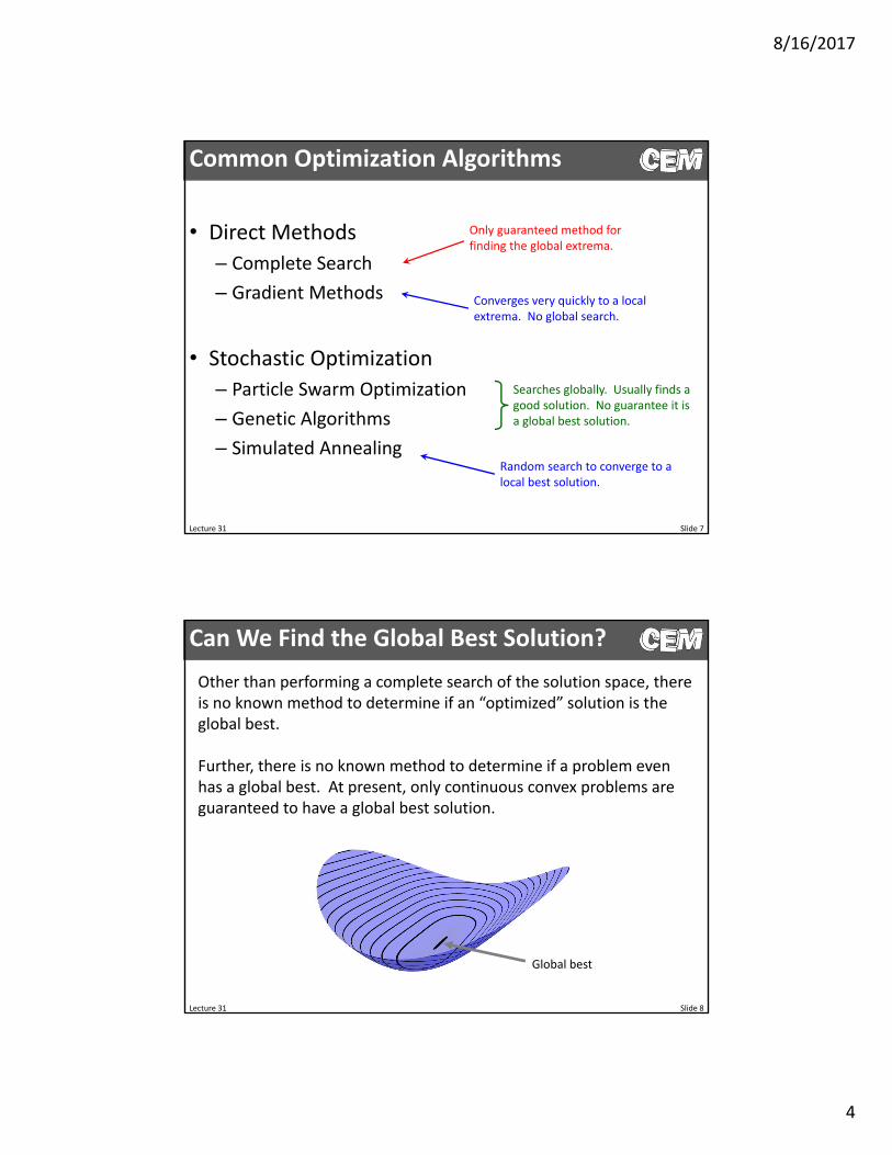
Can We Find the Global Best Solution?

Other than performing a complete search of the solution space, there is no known method to determine if an “optimized” solution is the global best.

Further, there is no known method to determine if a problem even has a global best.  At present, only continuous convex problems are guaranteed to have a global best solution.

Global best

8/16/2017

5

Lecture 31 Slide 9

Notes on Optimization

• Stochastic methods are used most effectively when very little is know about the solution space.  That is, when the engineer has no idea what the best design will look like.

• Unless something is known about the solution space, it is not possible to certify that the global best solution has been found.  As engineers, we are usually satisfied with “good enough” solutions.

• Only an exhaustive complete search can guarantee a global best solution has been found.

• Direct methods converge very fast, but can only find local best solutions.

• It’s all about the merit function, not the algorithm.

Lecture 31 Slide 10

The Merit Function

8/16/2017

6

Lecture 31 Slide 11

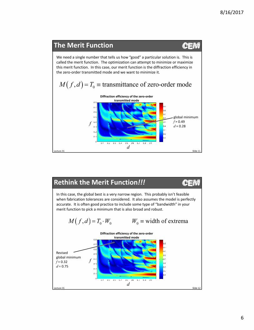
The Merit Function

We need a single number that tells us how “good” a particular solution is.  This is called the merit function.  The optimization can attempt to minimize or maximize this merit function.  In this case, our merit function is the diffraction efficiency in the zero‐order transmitted mode and we want to minimize it.

d

f

Diffraction efficiency of the zero‐order transmitted mode

global minimumf = 0.49d = 0.28

0, transmittance of zero-order modeM f d T

Lecture 31 Slide 12

Rethink the Merit Function!!!

In this case, the global best is a very narrow region.  This probably isn’t feasible when fabrication tolerances are considered.  It also assumes the model is perfectly accurate.  It is often good practice to include some type of “bandwidth” in your merit function to pick a minimum that is also broad and robust.

d

f

Diffraction efficiency of the zero‐order transmitted mode

Revisedglobal minimumf = 0.32d = 0.75

0 0,M f d T W 0 width of extremaW

8/16/2017

7

Lecture 31 13

Multiple Considerations

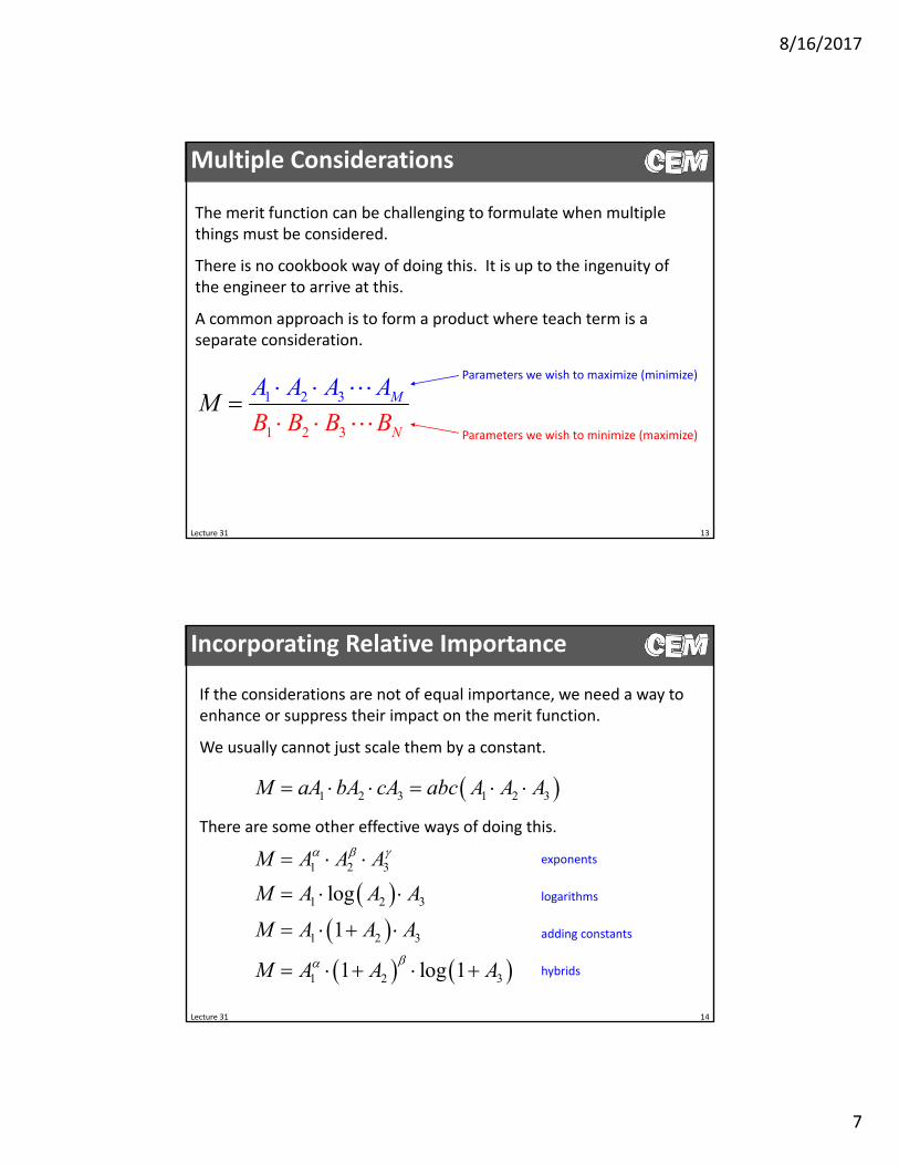
The merit function can be challenging to formulate when multiple things must be considered.

There is no cookbook way of doing this.  It is up to the ingenuity of the engineer to arrive at this.

A common approach is to form a product where teach term is a separate consideration.

2

2 3

1

1

3 M

N

MA A A A

B B B B

Parameters we wish to maximize (minimize)

Parameters we wish to minimize (maximize)

Lecture 31 14

Incorporating Relative Importance

If the considerations are not of equal importance, we need a way to enhance or suppress their impact on the merit function.

We usually cannot just scale them by a constant.

1 2 3 1 2 3M aA bA cA abc A A A

There are some other effective ways of doing this.

1 2 3

1 2 3

1 2 3

1 2 3

log

1

1 log 1

M A A A

M A A A

M A A A

M A A A

exponents

logarithms

adding constants

hybrids

8/16/2017

8

Lecture 31 15

Example (1 of 2)

Suppose we wish to optimize the design of an antenna.  

We are probably most concerned about its bandwidth B and efficiency E.  Based on this, we could define a merit function as

M B E Are these equally important?

The Shannon capacity theorem sets a limit on the bit rate C of data given the bandwidth B of the channel and the signal‐to‐noise ratio SNR.

2log 1 SNRC B This shows that bandwidth and efficiency are not equally important.

Lecture 31 16

Example (2 of 2)

We can come up with a better merit function that is inspired by the Shannon capacity theorem.

2log 1M B E Maybe size L is also a consideration.  We want data rate as high as possible using an antenna as small as possible.  A new merit function that considers size could be

2log 1B

M EL

This problem can be fixed by adding a constant to L.

2log 11

BM E

L

This merit function, however, would approach infinity as L approaches zero, leading to a false solution.

8/16/2017

9

Lecture 31 Slide 17

The “Rectangle” Algorithm

Lecture 31 18

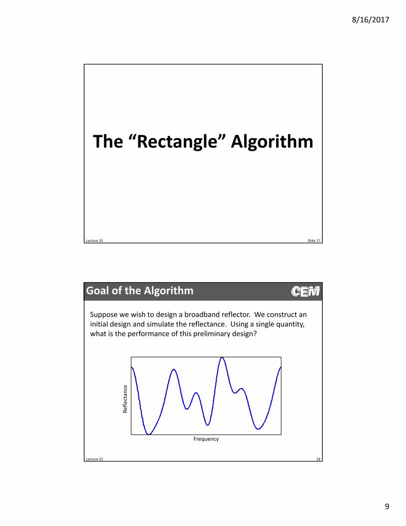
Goal of the Algorithm

Suppose we wish to design a broadband reflector.  We construct an initial design and simulate the reflectance.  Using a single quantity, what is the performance of this preliminary design?

Frequency

Reflectan

ce

8/16/2017

10

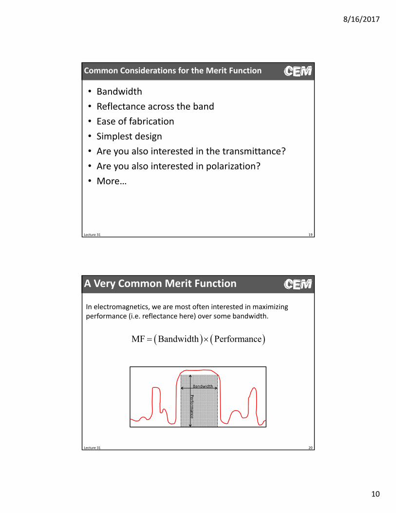
Common Considerations for the Merit Function

• Bandwidth

• Reflectance across the band

• Ease of fabrication

• Simplest design

• Are you also interested in the transmittance?

• Are you also interested in polarization?

• More…

Lecture 31 19

Lecture 31 20

A Very Common Merit Function

In electromagnetics, we are most often interested in maximizing performance (i.e. reflectance here) over some bandwidth.

MF Bandwidth Performance

Bandwidth

Perform

ance

8/16/2017

11

The Rectangle Algorithm

Lecture 31 21

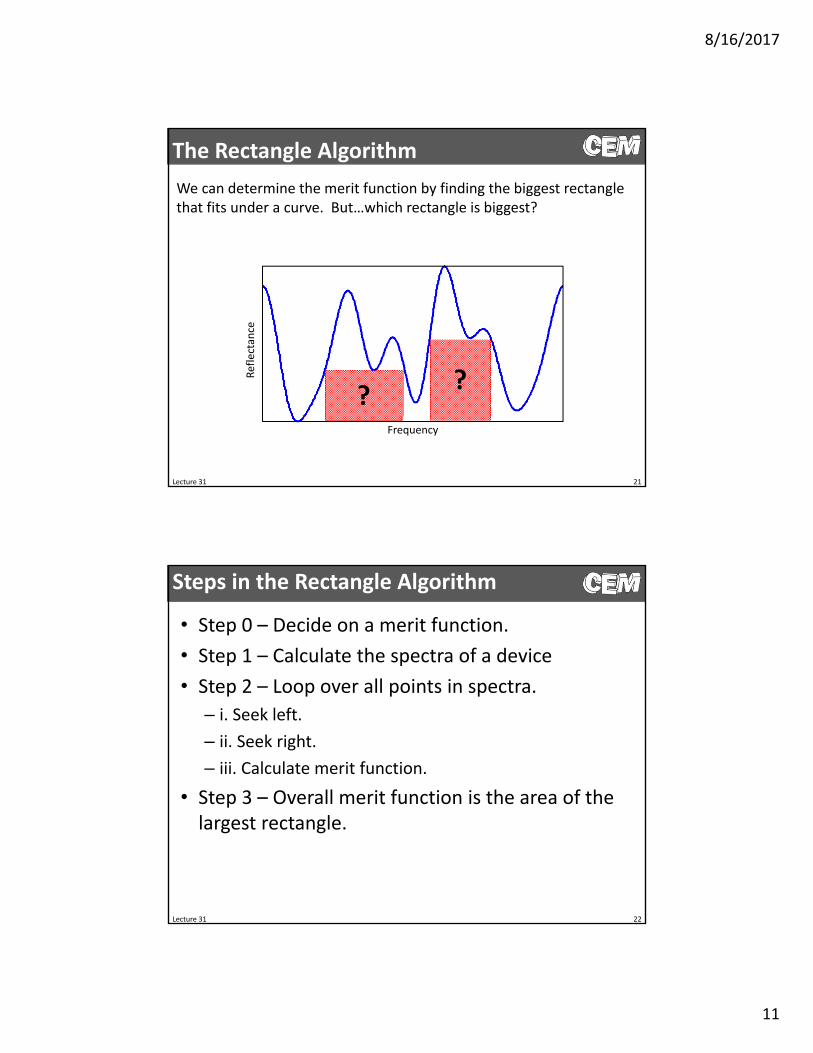
We can determine the merit function by finding the biggest rectangle that fits under a curve.  But…which rectangle is biggest?

Frequency

Reflectan

ce

??

Steps in the Rectangle Algorithm

• Step 0 – Decide on a merit function.

• Step 1 – Calculate the spectra of a device

• Step 2 – Loop over all points in spectra.

– i. Seek left.

– ii. Seek right.

– iii. Calculate merit function.

• Step 3 – Overall merit function is the area of the largest rectangle.

Lecture 31 22

8/16/2017

12

Lecture 31 23

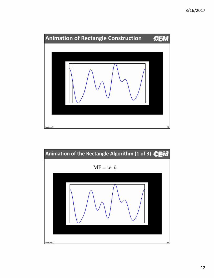
Animation of Rectangle Construction

Lecture 31 24

Animation of the Rectangle Algorithm (1 of 3)

MF w h

8/16/2017

13

Lecture 31 25

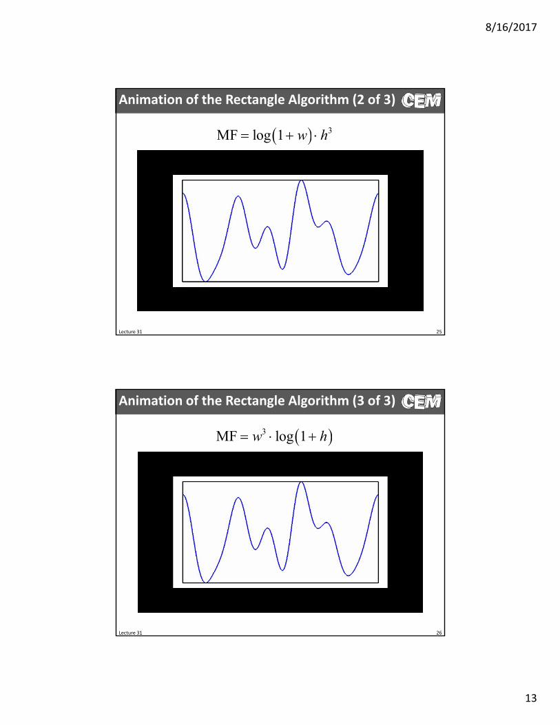
Animation of the Rectangle Algorithm (2 of 3)

3MF log 1 w h

Lecture 31 26

Animation of the Rectangle Algorithm (3 of 3)

3MF log 1w h

8/16/2017

14

Lecture 31 Slide 27

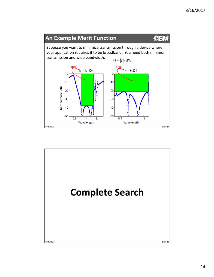
An Example Merit Function

Suppose you want to minimize transmission through a device where your application requires it to be broadband.  You need both minimum transmission and wide bandwidth.

Tran

smittance (dB)

Wavelength Wavelength

BWM T area area

Lecture 31 Slide 28

Complete Search

8/16/2017

15

Lecture 31 Slide 29

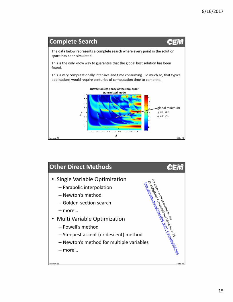
Complete Search

The data below represents a complete search where every point in the solution space has been simulated.

This is the only know way to guarantee that the global best solution has been found.

This is very computationally intensive and time consuming.  So much so, that typical applications would require centuries of computation time to complete.

d

f

Diffraction efficiency of the zero‐order transmitted mode

global minimumf = 0.49d = 0.28

Other Direct Methods

• Single Variable Optimization

– Parabolic interpolation

– Newton’s method

– Golden‐section search

– more…

• Multi Variable Optimization

– Powell’s method

– Steepest ascent (or descent) method

– Newton’s method for multiple variables

– more…

Lecture 31 Slide 30

8/16/2017

16

Lecture 31 Slide 31

Genetic Algorithms

Lecture 31 Slide 32

What are Genetic Algorithms?

Genetic algorithms code designs into “chromosomes.”  A population of candidate designs are simulated.  Chromosomes are interchanged between the best few designs to produce the next generation of candidate designs.  This process continues until convergence.

Parent #2 01011010101100101010

1010 1010Child #1

Child #2

Parent #1 10010011010100110101

1001 01010011

1

Chil

1100

010 0101 0101

001001101 110101

10d # 01 1 13 000

8/16/2017

17

Lecture 31 Slide 33

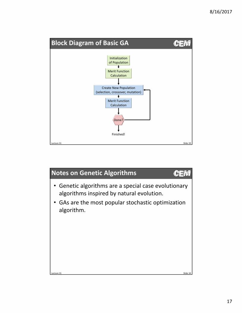
Block Diagram of Basic GA

Initialization of Population

Merit Function Calculation

Create New Population (selection, crossover, mutation)

Merit Function Calculation

Done?

Finished!

Notes on Genetic Algorithms

• Genetic algorithms are a special case evolutionary algorithms inspired by natural evolution.

• GAs are the most popular stochastic optimization algorithm.

Lecture 31 Slide 34

8/16/2017

18

Lecture 31 Slide 35

Simulated Annealing

Lecture 31 Slide 36

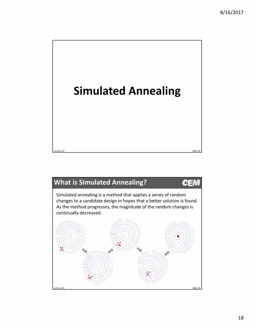
What is Simulated Annealing?

Simulated annealing is a method that applies a series of random changes to a candidate design in hopes that a better solution is found.  As the method progresses, the magnitude of the random changes is continually decreased.  

8/16/2017

19

Lecture 31 Slide 37

Block Diagram of SA

Notes on Simulated Annealing

• Name is derived from annealing commonly employed in metallurgy.  A series of heating and cooling cycles reduces defects in crystals.

• Usually used to “fine tune” a design.

• Can still be used for global optimization.

Lecture 31 Slide 38

8/16/2017

20

Lecture 31 Slide 39

Particle Swarm Optimization

Lecture 31 Slide 40

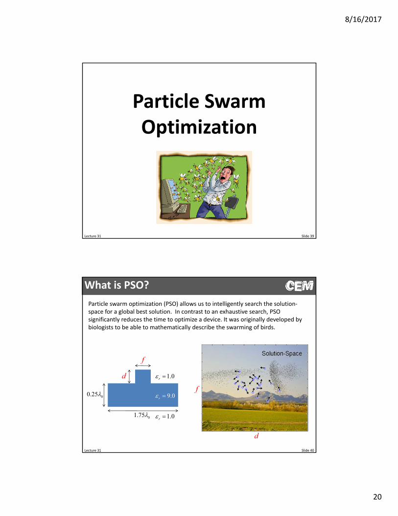
What is PSO?

Particle swarm optimization (PSO) allows us to intelligently search the solution‐space for a global best solution.  In contrast to an exhaustive search, PSO significantly reduces the time to optimize a device. It was originally developed by biologists to be able to mathematically describe the swarming of birds.

d

f

d

9.0r

1.0r

1.0r

01.75

f

00.25

8/16/2017

21

Lecture 31 Slide 41

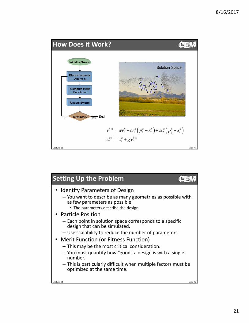
How Does it Work?

11 2

1 1

k k k k k k k ki i i i g i

k k ki i i

v wv cr p x sr p x

x x v

Setting Up the Problem

• Identify Parameters of Design– You want to describe as many geometries as possible with as few parameters as possible• The parameters describe the design.

• Particle Position– Each point in solution space corresponds to a specific design that can be simulated.

– Use scalability to reduce the number of parameters

• Merit Function (or Fitness Function)– This may be the most critical consideration.– You must quantify how “good” a design is with a single number.

– This is particularly difficult when multiple factors must be optimized at the same time.

Lecture 31 Slide 42

8/16/2017

22

Lecture 31 Slide 43

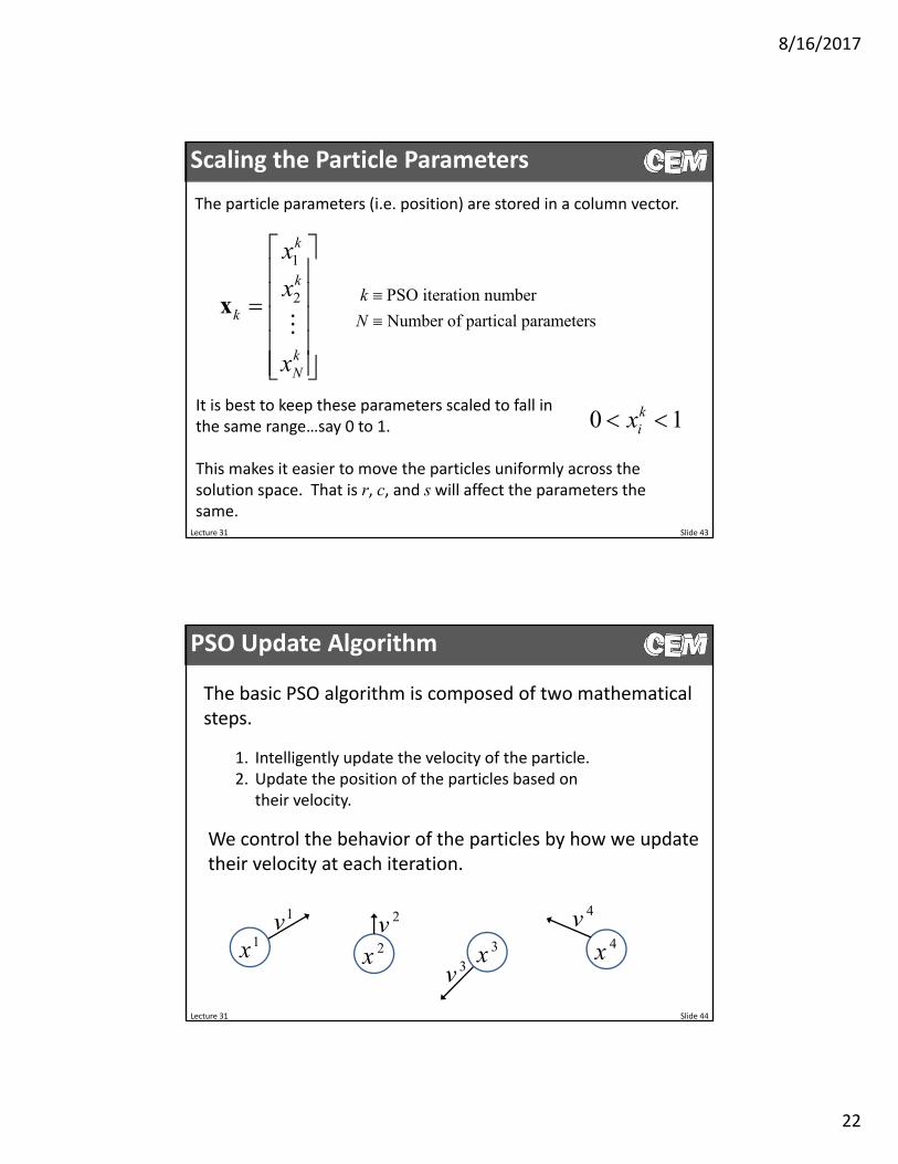
Scaling the Particle Parameters

The particle parameters (i.e. position) are stored in a column vector.

1

2

k

k

k

kN

x

x

x

x

PSO iteration number

Number of partical parameters

k

N

It is best to keep these parameters scaled to fall in the same range…say 0 to 1.

This makes it easier to move the particles uniformly across the solution space.  That is r, c, and s will affect the parameters the same.

0 1kix

PSO Update Algorithm

Lecture 31 Slide 44

The basic PSO algorithm is composed of two mathematical steps.

1. Intelligently update the velocity of the particle.2. Update the position of the particles based on 

their velocity.

We control the behavior of the particles by how we update their velocity at each iteration.

1x

1v2x

2v3x

3v4x

4v

8/16/2017

23

PSO Velocity Update

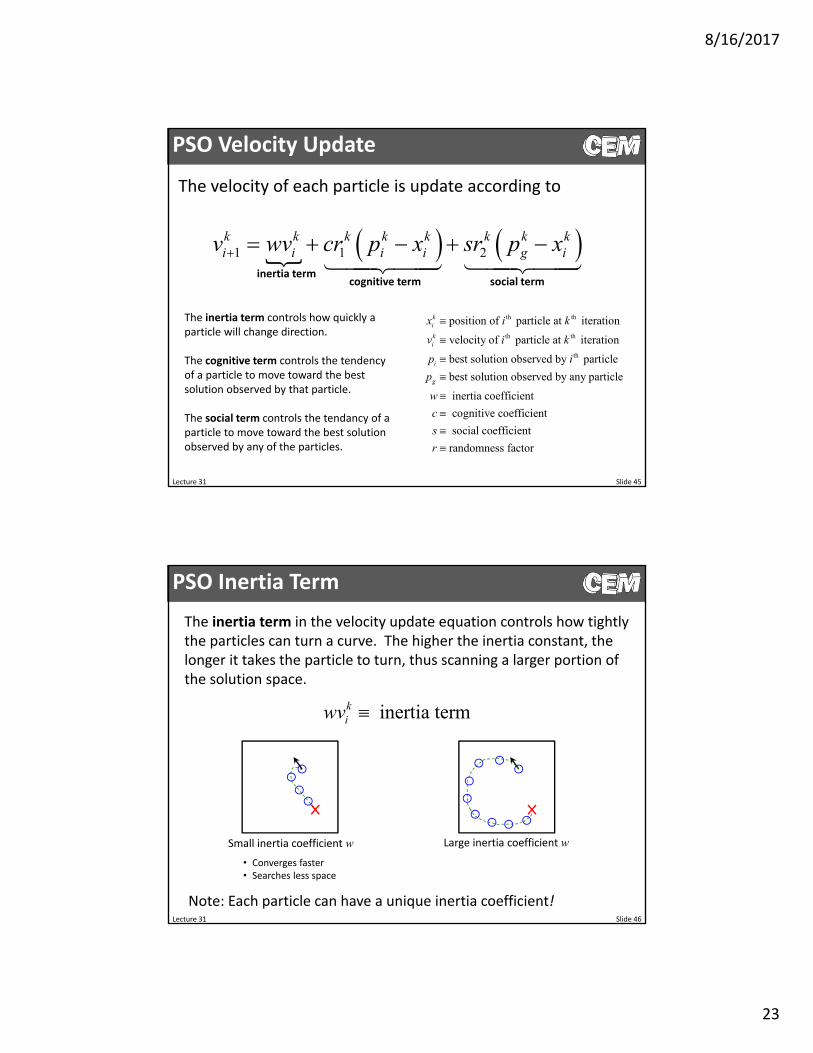
The velocity of each particle is update according to

Lecture 31 Slide 45

th th

th th

th

position of particle at iteration

velocity of particle at iteration

best solution observed by particle

best solution observed by any particle

inertia coefficient

cog

ki

ki

i

g

x i k

v i k

p i

p

w

c

nitive coefficient

social coefficient

randomness factor

s

r

1 1 2k k k k k k k ki i i i g iv wv cr p x sr p x

inertia term

cognitive term social term

The inertia term controls how quickly a particle will change direction.

The cognitive term controls the tendency of a particle to move toward the best solution observed by that particle.

The social term controls the tendancy of a particle to move toward the best solution observed by any of the particles.

PSO Inertia Term

Lecture 31 Slide 46

The inertia term in the velocity update equation controls how tightly the particles can turn a curve.  The higher the inertia constant, the longer it takes the particle to turn, thus scanning a larger portion of the solution space.

inertia termkiwv

Note: Each particle can have a unique inertia coefficient!

Small inertia coefficient w Large inertia coefficient w

• Converges faster• Searches less space

8/16/2017

24

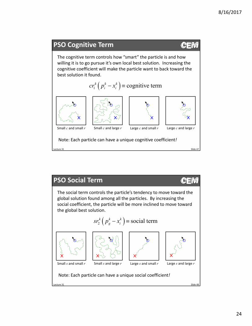
PSO Cognitive Term

Lecture 31 Slide 47

The cognitive term controls how “smart” the particle is and how willing it is to go pursue it’s own local best solution.  Increasing the cognitive coefficient will make the particle want to back toward the best solution it found.

1 cognitive termk k ki icr p x

Note: Each particle can have a unique cognitive coefficient!

Small c and small r Small c and large r Large c and small r Large c and large r

PSO Social Term

Lecture 31 Slide 48

The social term controls the particle’s tendency to move toward the global solution found among all the particles.  By increasing the social coefficient, the particle will be more inclined to move toward the global best solution.

2 social termk k kg isr p x

Note: Each particle can have a unique social coefficient!

Small s and small r Small s and large r Large s and small r Large s and large r

8/16/2017

25

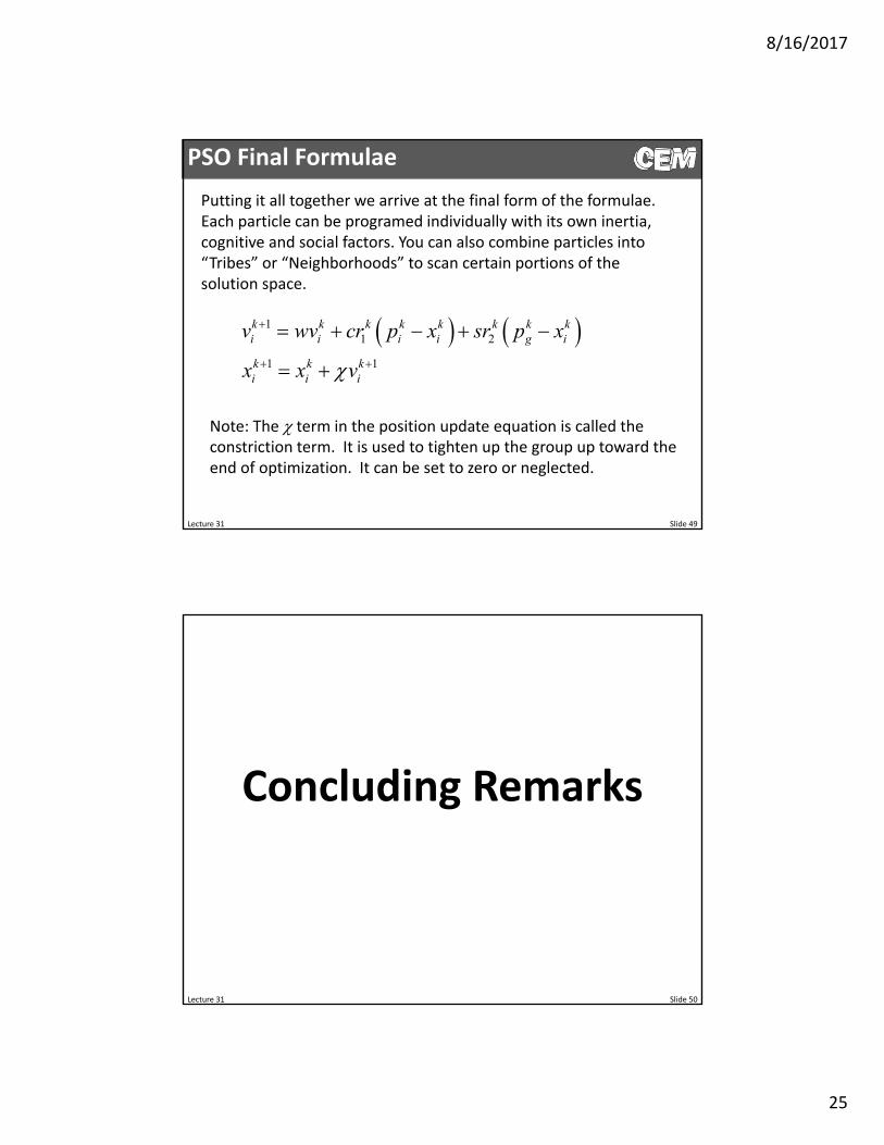
PSO Final Formulae

Lecture 31 Slide 49

11 2

1 1

k k k k k k k ki i i i g i

k k ki i i

v wv cr p x sr p x

x x v

Putting it all together we arrive at the final form of the formulae. Each particle can be programed individually with its own inertia, cognitive and social factors. You can also combine particles into “Tribes” or “Neighborhoods” to scan certain portions of the solution space.

Note: The  term in the position update equation is called the constriction term.  It is used to tighten up the group up toward the end of optimization.  It can be set to zero or neglected.

Lecture 31 Slide 50

Concluding Remarks

8/16/2017

26

Final Remarks

• Almost never a guarantee a global best solution has been found.

• Dr. Rumpf tends to apply the methods this way…– Continuous design variables  Particle swarm optimization

– Discrete design variables  Genetic algorithm

– Fine tuning a solution  Simulated annealing, gradient descent, Newton’s method

Lecture 31 Slide 51