Lecture : 3 (APPLICATIONS OF LAPLACE TRANSFORMS)...Lecture : 3 (APPLICATIONS OF LAPLACE TRANSFORMS) Course : B.Sc. (H) Physics Semester : IV Subject : Mathematical Physics III UPC

1

Lecture : 3

(APPLICATIONS OF LAPLACE TRANSFORMS)

Course : B.Sc. (H) Physics Semester : IV Subject : Mathematical Physics III UPC : 32221401 Teacher : Ms. Bhavna Vidhani

(Deptt. of Physics & Electronics)

Topics covered in this lecture:- Applications of LT to Second order Differential equations, Coupled Differential

equations & solution of heat flow along semi-infinite bar

3.1 Ordinary Differential equations with constant coefficients: Ordinary Differential equations with constant coefficients can be very easily solved using Laplace transform without finding the general solution and the arbitrary constants. Examples: 1. Solve y ‒ 2 y + 2 y = 0, given y = y = 1 when t = 0. Sol. We have, y ‒ 2 y + 2 y = 0 (1) Taking Laplace transform of both sides of eq. (1), we get L { y } ‒ 2 L { y } + 2 L { y } = L {0} [ 2s L { y } ‒ s )0(y ‒ )0(y ] ‒ 2[ s L { y } ‒ )0(y ] + 2 L { y } = 0 [ L { )(tf } = )0()( fsFs and L { )(tf } = 2s )(sF ‒ s )0(f ‒ )0(f ] ( 2s ‒ 2 s + 2) L { y } ‒ ( s ‒ 2) 1 ‒ (1) = 0 [ )0(y = )0(y = 1]

L { y } = 22

12

sss =

1)1(1

2

ss (2)

Taking Inverse Laplace transform of both sides of eq. (2), we get

y = 1L

1)1(1

2ss

= te 1L

22 1ss = te tcos , the required solution.

2. Using Laplace Transform method, solve 2

2

dtyd + y = t , given 2

2

dtyd = 1, when t = 0 and

y = 0 when t = .

Sol. We have, 2

2

dtyd + y = t (1)

Taking Laplace transform of both sides of eq. (1), we get

2

L

2

2

dtyd + L { y } = L { t }

[ 2s L { y } ‒ s )0(y ‒ )0(y ] + L { y } = 21s

[ L { )(tf } = )0()( fsFs and L { )(tf } = 2s )(sF ‒ s )0(f ‒ )0(f ]

( 2s + 1) L { y } ‒ s )0(y ‒ )0(y = 21s

(2)

Now, let at t = 0, )0(y = a and )0(y = 1 (given) (3) Put eq. (3) in eq. (2), we get

( 2s + 1) L { y } ‒ s a ‒ 1 = 21s

L { y } = 12 s

as + 1

12 s

+ )1(

122 ss

(4)


y = a 1L

12ss + 1L

11

2s + 1L

)1(122 ss

y = a tcos + tsin + 1L

)1(122 ss

(5)

Now, 1L

)1(122 ss

= 1L

111

22 ss

= 1L

21s

‒ 1L

22 11

s

= t ‒ tsin (6) Put eq. (6) in eq. (5), we get y = a tcos + tsin + t ‒ tsin = t + a tcos (7) Now, y = 0 when t = 0 = + a cos 0 = + a (‒1) a = Put a = in eq. (7), we get y = t + tcos , the required solution. 3. Solve y ‒ 3 y + 3 y ‒ y = 2t te , given )0(y = 1, )0(y = 0, )0(y = ‒ 2. Sol. We have, y ‒ 3 y + 3 y ‒ y = 2t te (1) Taking Laplace transform of both sides of eq. (1), we get L { y } ‒ 3 L { y } + 3 L { y } ‒ L { y } = L { 2t te } [ 3s L { y } ‒

2s )0(y ‒ s )0(y ‒ )0(y ] ‒ 3 [2s L { y } ‒ s )0(y ‒ )0(y ] + 3 [ s L { y }

‒ )0(y ] ‒ L { y } = 2)1(

11

2

2

sdsd

[ L { )(tf } = )0()( fsFs , L { )(tf } = 2s )(sF ‒ s )0(f ‒ )0(f , L { )(tf } = 3s )(sF ‒

2s )0(f ‒ s )0(f ‒ )0(f , and

3

L { nt )(tf } = n)1( n

n

dssFd )( ]

[ 3s L { y } ‒ 2s (1) ‒ s (0) ‒ (‒ 2)] ‒ 3 [ 2s L { y } ‒ s (1) ‒ (0)] + 3 [ s L { y } ‒ (1)]

‒ L { y } = 3)1(2s

[ )0(y = 1, )0(y = 0, )0(y = ‒ 2]

( 3s ‒ 3 2s + 3 s ‒ 1) L { y } ‒ 2s + 3 s ‒ 1 = 3)1(2s

( 3s ‒ 3 2s + 3 s ‒ 1) L { y } = 3)1(2s

+ 2s ‒ 3 s + 1

L { y } = )133()1(

2233 ssss

+ )133(

1323

2

sssss

L { y } = 33 )1()1(2

ss + 3

2

)1(13

sss

y = 1L

6)1(2

s + 1L

3

2

)1(1)1()1(

sss

y = te 1L

62s

+ te 1L

3

2 1sss [ 1L { )( bsF } = bte 1L { )(sF }]

y = 2 te 1L

61s

+ te 1L

32111sss

y = 2 te!5

5t + te

21

2tt

!)1(1 1

1

nt

sL

n

n

y = te

6021

52 ttt , the required solution.

3.2 Ordinary Differential equations with variable coefficients: Ordinary Differential equations with variable coefficients can be very easily solved using Laplace transform. Examples: 1. Using Laplace Transform, solve the following differential equation y + 2 t y ‒ y = t , when )0(y = 0, )0(y = 1 Sol. We have, y + 2 t y ‒ y = t (1) Taking Laplace transform of both sides of eq. (1), we get L { y } + 2 L { t y } ‒ L { y } = L { t }

[ 2s L { y } ‒ s )0(y ‒ )0(y ] ‒ 2dsd

[ s L { y } ‒ )0(y ] ‒ L { y } = 21s

[ L { )(tf } = )0()( fsFs , L { )(tf } = 2s )(sF ‒ s )0(f ‒ )0(f ]

[ 2s L { y } ‒ s (0) ‒ (1)] ‒ 2dsd

[ s L { y } ‒ 0] ‒ L { y } = 21s

[ )0(y = 0, )0(y = 1]

4

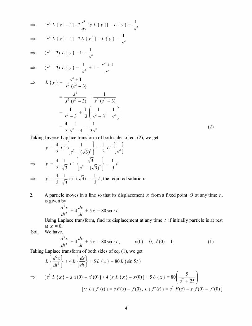
[ 2s L { y } ‒ 1] ‒ 2dsd

[ s L { y }] ‒ L { y } = 21s

[ 2s L { y } ‒ 1] ‒ 2 L { y }] ‒ L { y } = 21s

( 2s ‒ 3) L { y } ‒ 1 = 21s

( 2s ‒ 3) L { y } = 21s

+ 1 = 2

2 1s

s

L { y } = )3(

122

2

sss

= )3( 22

2

sss +

)3(122 ss

= 3

12 s

+ 31

221

31

ss

= 34

31

2 s ‒ 23

1s

(2)


y = 34 1L

22 )3(1

s ‒

31 1L

21s

y = 34

31 1L

22 )3(3

s ‒

31 t

y = 34

31 t3sinh ‒

31 t , the required solution.

2. A particle moves in a line so that its displacement x from a fixed point O at any time t , is given by

2

2

dtxd + 4

dtdx + 5 x = 80 t5sin

Using Laplace transform, find its displacement at any time t if initially particle is at rest at x = 0. Sol. We have,

2

2

dtxd + 4

dtdx + 5 x = 80 t5sin , )0(x = 0, )0(x = 0 (1)


L

2

2

dtxd + 4 L

dtdx + 5 L { x } = 80 L { t5sin }

[ 2s L { x } ‒ s )0(x ‒ )0(x ] + 4 [ s L { x } ‒ )0(x ] + 5 L { x } = 80

255

2s

[ L { )(tf } = )0()( fsFs , L { )(tf } = 2s )(sF ‒ s )0(f ‒ )0(f ]

5

[ 2s L { x } ‒ s (0) ‒ 0)] + 4 [ s L { x } ‒ 0] + 5 L { x } = 25

4002 s

[ )0(x = 0, )0(x = 0]

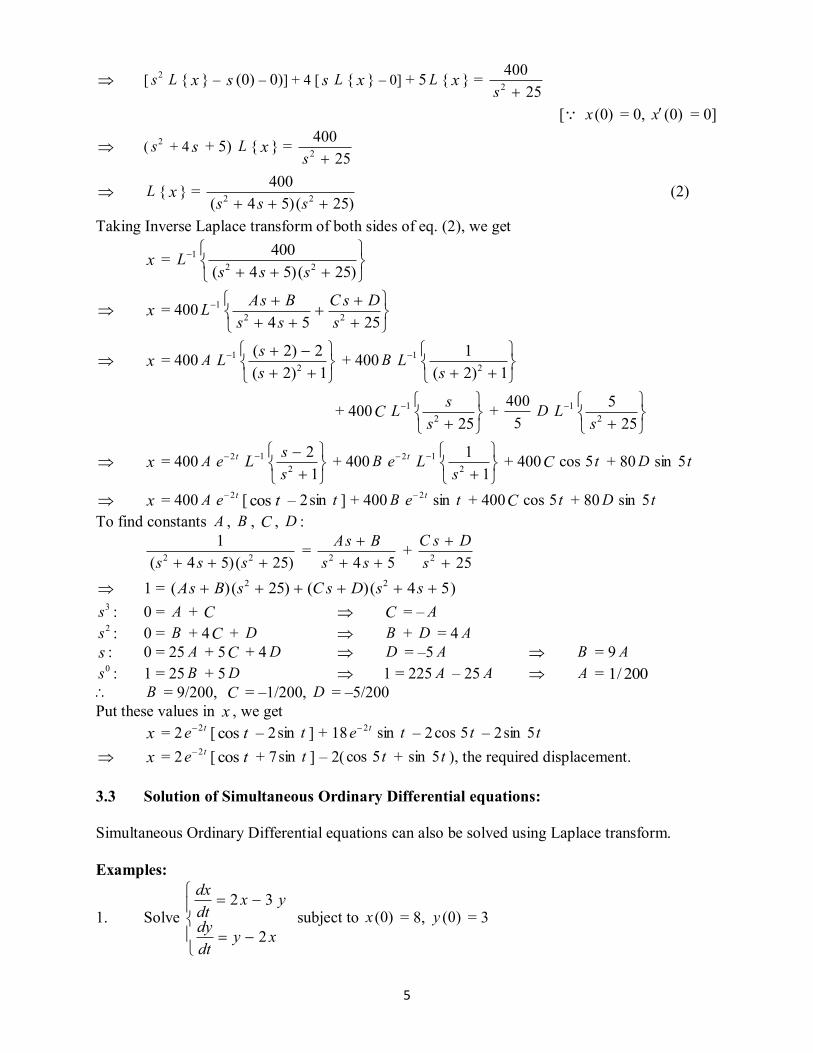
( 2s + 4 s + 5) L { x } = 25

4002 s

L { x } = )25()54(

40022 sss

(2)


x = 1L

)25()54(400

22 sss

x = 400 1L

2554 22 sDsC

ssBsA

x = 400 A 1L

1)2(2)2(

2ss + 400 B 1L

1)2(1

2s

+ 400C 1L

252ss +

5400 D 1L

255

2s

x = 400 A te 2 1L

12

2ss + 400 B te 2 1L

11

2s + 400C t5cos + 80 D t5sin

x = 400 A te 2 [ tcos ‒ 2 tsin ] + 400 B te 2 tsin + 400C t5cos + 80 D t5sin To find constants A , B , C , D :

)25()54(

122 sss

= 542

ssBsA +

252

sDsC

1 = )54()()25()( 22 ssDsCsBsA 3s : 0 = A + C C = ‒ A 2s : 0 = B + 4C + D B + D = 4 A

s : 0 = 25 A + 5C + 4 D D = ‒5 A B = 9 A 0s : 1 = 25 B + 5 D 1 = 225 A ‒ 25 A A = 200/1

B = 9/200, C = ‒1/200, D = ‒5/200 Put these values in x , we get x = 2 te 2 [ tcos ‒ 2 tsin ] + 18 te 2 tsin ‒ 2 t5cos ‒ 2 t5sin x = 2 te 2 [ tcos + 7 tsin ] ‒ 2( t5cos + t5sin ), the required displacement. 3.3 Solution of Simultaneous Ordinary Differential equations: Simultaneous Ordinary Differential equations can also be solved using Laplace transform. Examples:

1. Solve

xydtdy

yxdtdx

2

32 subject to )0(x = 8, )0(y = 3

6

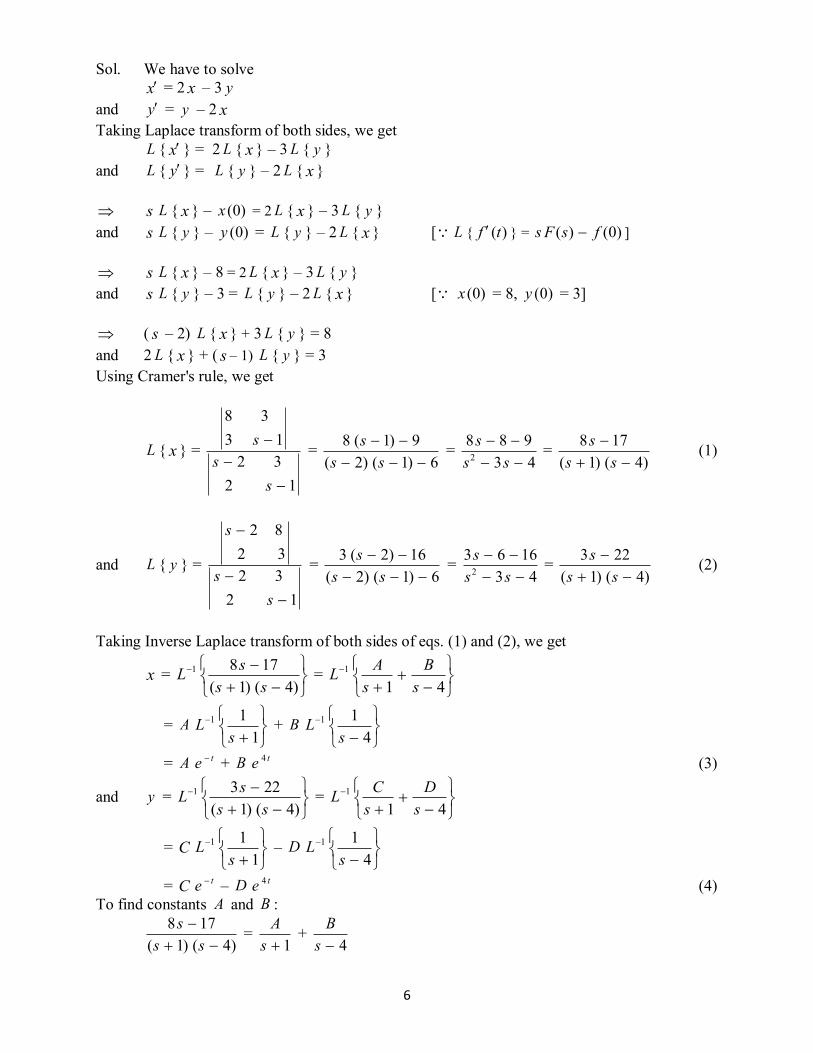
Sol. We have to solve x = 2 x ‒ 3 y and y = y ‒ 2 x Taking Laplace transform of both sides, we get L { x } = 2 L { x } ‒ 3 L { y } and L { y } = L { y } ‒ 2 L { x } s L { x } ‒ )0(x = 2 L { x } ‒ 3 L { y } and s L { y } ‒ )0(y = L { y } ‒ 2 L { x } [ L { )(tf } = )0()( fsFs ] s L { x } ‒ 8 = 2 L { x } ‒ 3 L { y } and s L { y } ‒ 3 = L { y } ‒ 2 L { x } [ )0(x = 8, )0(y = 3] ( s ‒ 2) L { x } + 3 L { y } = 8 and 2 L { x } + ( s ‒ 1) L { y } = 3 Using Cramer's rule, we get

L { x } =

123213

38

ss

s =

6)1()2(9)1(8

sss =

43988

2

sss =

)4()1(178

sss (1)

and L { y } =

12323282

ss

s

= 6)1()2(

16)2(3

sss =

431663

2

sss =

)4()1(223

sss (2)

Taking Inverse Laplace transform of both sides of eqs. (1) and (2), we get

x = 1L

)4()1(178ss

s = 1L

41 sB

sA

= A 1L

11

s + B 1L

41

s

= A te + B te 4 (3)

and y = 1L

)4()1(223ss

s = 1L

41 sD

sC

= C 1L

11

s ‒ D 1L

41

s

= C te ‒ D te 4 (4) To find constants A and B :

)4()1(

178

sss =

1sA +

4sB

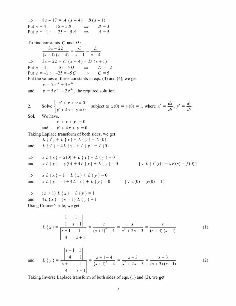
7

178 s = A ( 4s ) + B ( 1s ) Put s = 4 : 15 = 5 B B = 3 Put s = ‒1 : ‒25 = ‒5 A A = 5 To find constants C and D :

)4()1(

223

sss =

1sC ‒

4sD

223 s = C ( 4s ) + D ( 1s ) Put s = 4 : ‒10 = 5 D D = ‒2 Put s = ‒1 : ‒25 = ‒5C C = 5 Put the values of these constants in eqs. (3) and (4), we get x = 5 te + 3 te 4 and y = 5 te ‒ 2 te 4 , the required solution.

2. Solve

040

yxyyxx

subject to )0(x = )0(y = 1, where x = dtdx , y =

dtdy

Sol. We have, yxx = 0 and yxy 4 = 0 Taking Laplace transform of both sides, we get L { x} + L { x } + L { y } = L {0} and L { y} + 4 L { x } + L { y } = L {0} s L { x } ‒ )0(x + L { x } + L { y } = 0 and s L { y } ‒ )0(y + 4 L { x } + L { y } = 0 [ L { )(tf } = )0()( fsFs ] s L { x } ‒ 1 + L { x } + L { y } = 0 and s L { y } ‒ 1 + 4 L { x } + L { y } = 0 [ )0(x = )0(y = 1] ( s + 1) L { x } + L { y } = 1 and 4 L { x } + ( s + 1) L { y } = 1 Using Cramer's rule, we get

L { x } =

141111

11

ss

s =

4)1( 2 ss =

322 sss =

)1()3( sss (1)

and L { y } =

14111411

ss

s

= 4)1(

412

ss =

323

2

sss =

)1()3(3

sss (2)

Taking Inverse Laplace transform of both sides of eqs. (1) and (2), we get

8

x = 1L

)1()3( sss = 1L

13 sB

sA

= A 1L

31

s + B 1L

11

s

= A te 3 + B te (3)

and y = 1L

)1()3(3ss

s = 1L

13 sD

sC

= C 1L

31

s + D 1L

11

s

= C te 3 + D te (4) To find constants A and B :

)1()3( ss

s = 3s

A + 1s

B

s = A ( 1s ) + B ( 3s ) Put s = 1 : 1 = 4 B B = 1/4 Put s = ‒3 : ‒3 = ‒4 A A = 3/4 To find constants C and D :

)1()3(

3

sss =

3sC +

1sD

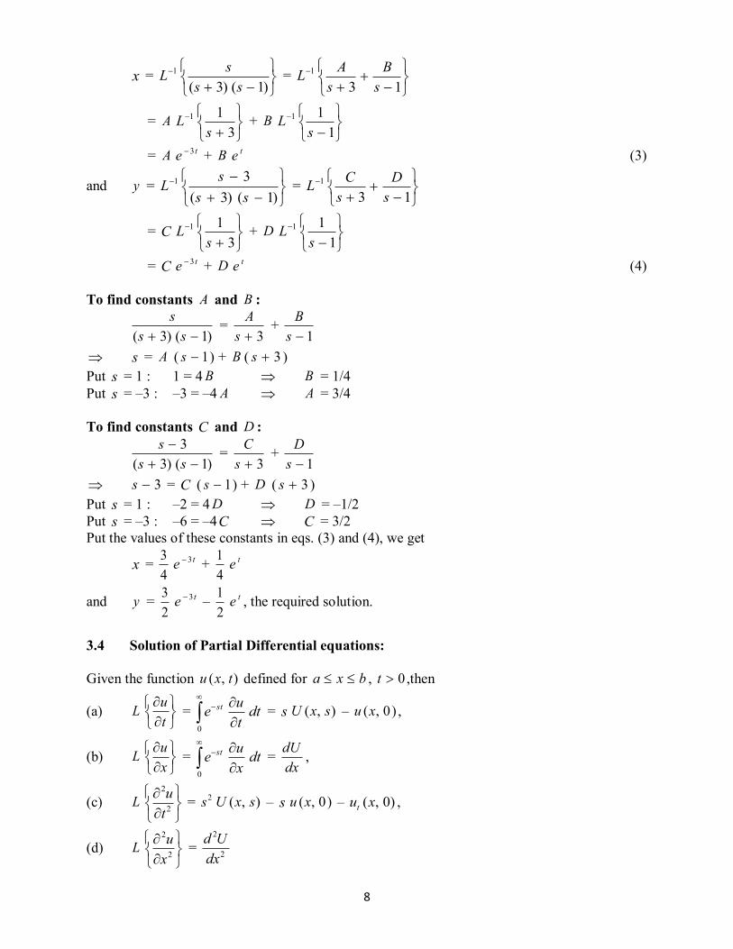
3s = C ( 1s ) + D ( 3s ) Put s = 1 : ‒2 = 4 D D = ‒1/2 Put s = ‒3 : ‒6 = ‒4C C = 3/2 Put the values of these constants in eqs. (3) and (4), we get

x = 43 te 3 +

41 te

and y = 23 te 3 ‒

21 te , the required solution.

3.4 Solution of Partial Differential equations: Given the function ),( txu defined for bxa , 0t ,then

(a) L

tu = dt

tue st

0

= s ),( sxU ‒ )0,(xu ,

(b) L

xu = dt

xue st

0

= dxdU ,

(c) L

2

2

tu = 2s ),( sxU ‒ s )0,(xu ‒ )0,(xut ,

(d) L

2

2

xu = 2

2

dxUd

9

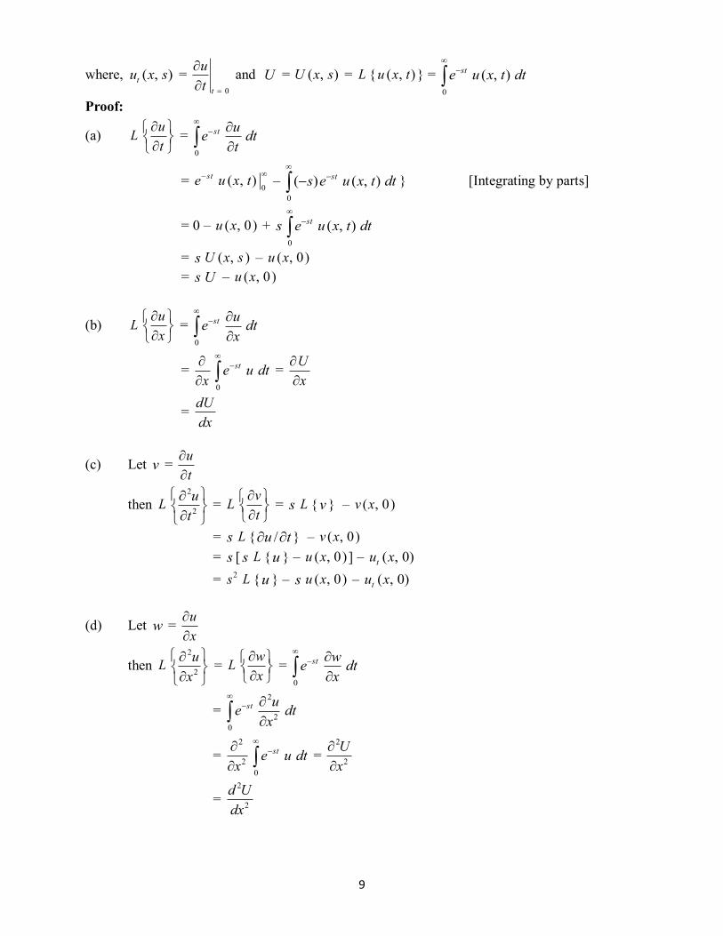
where, ),( sxut = 0

ttu and U = ),( sxU = L { ),( txu } = dttxue st

0

),(

Proof:

(a) L

tu = dt

tue st

0

=

0),( txue st ‒ dttxues st

0

),()( } [Integrating by parts]

= 0 ‒ )0,(xu + s dttxue st

0

),(

= s ),( sxU ‒ )0,(xu = s U ‒ )0,(xu

(b) L

xu = dt

xue st

0

= x dtue st

0

= xU

= dxdU

(c) Let v = tu

then L

2

2

tu = L

tv = s L { v } ‒ )0,(xv

= s L { tu / } ‒ )0,(xv = s [ s L {u } ‒ )0,(xu ] ‒ )0,(xut = 2s L {u } ‒ s )0,(xu ‒ )0,(xut

(d) Let w = xu

then L

2

2

xu = L

xw = dt

xwe st

0

= dtxue st

02

2

= 2

2

x dtue st

0

= 2

2

xU

= 2

2

dxUd

10

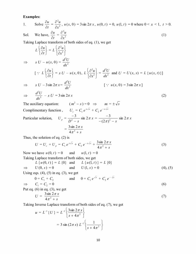
Examples:

1. Solve tu

= 2

2

xu

, )0,(xu = 3 x2sin , ),0( tu = 0, ),1( tu = 0 where 0 < x < 1, t > 0.

Sol. We have, tu

= 2

2

xu

(1)


L

tu = L

2

2

xu

s U ‒ )0,(xu = 2

2

dxUd

[ L

tu = s U ‒ )0,(xu , L

2

2

xu = 2

2

dxUd and U = ),( sxU = L { ),( txu }]

s U ‒ 3 x2sin = 2

2

dxUd [ )0,(xu = 3 x2sin ]

2

2

dxUd ‒ s U = 3 x2sin (2)

The auxiliary equation: ( sm 2 ) = 0 m = s

Complimentary function , cU = 1C sxe + 2C sxe

Particular solution, pU = sD

2

3 x2sin = s

2)2(3

x2sin

= sx

242sin3

Thus, the solution of eq. (2) is

U = cU + pU = 1C sxe + 2C sxe + sx

242sin3

(3)

Now we have ),0( tu = 0 and ),1( tu = 0 Taking Laplace transform of both sides, we get L { ),0( tu } = L {0} and L { ),1( tu } = L {0} ),0( sU = 0 and ),1( sU = 0 (4), (5) Using eqs. (4), (5) in eq. (3), we get 0 = 1C + 2C and 0 = 1C se + 2C se 1C = 2C = 0 (6) Put eq. (6) in eq. (3), we get

U = sx

242sin3

(7)


u = 1L {U } = 1L

242sin3

sx

= )2(sin3 x 1L

241s

11

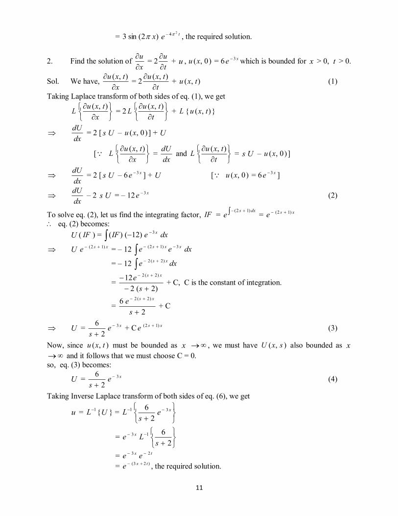
= )2(sin3 x te24 , the required solution.

2. Find the solution of xu

= 2tu

+ u , )0,(xu = 6 xe 3 which is bounded for x > 0, t > 0.

Sol. We have, x

txu

),( = 2t

txu

),( + ),( txu (1)


L

xtxu ),( = 2 L

ttxu ),( + L { ),( txu }

dxdU = 2 [ s U ‒ )0,(xu ] + U

[ L

xtxu ),( =

dxdU and L

ttxu ),( = s U ‒ )0,(xu ]

dxdU = 2 [ s U ‒ 6 xe 3 ] + U [ )0,(xu = 6 xe 3 ]

dxdU ‒ 2 s U = ‒ 12 xe 3 (2)

To solve eq. (2), let us find the integrating factor, IF = dxse

)12( = xse )12( eq. (2) becomes: U ( IF ) = dxeIF x3)12()(

U xse )12( = ‒ 12 dxee xxs 3)12(

= ‒ 12 dxe xs

)2(2

= )2(2

12 )2(2

se xs

+ C, C is the constant of integration.

= 2

6 )2(2

se xs

+ C

U = 2

6s

xe 3 + C xse )12( (3)

Now, since ),( txu must be bounded as x , we must have ),( sxU also bounded as x and it follows that we must choose C = 0. so, eq. (3) becomes:

U = 2

6s

xe 3 (4)


u = 1L {U } = 1L

xes

3

26

= xe 3 1L

26

s

= xe 3 te 2 = )23( txe , the required solution.

12

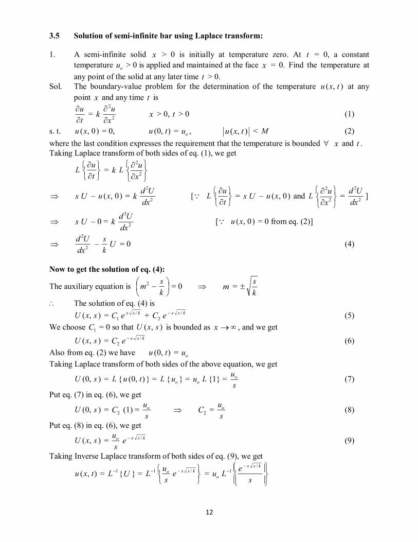
3.5 Solution of semi-infinite bar using Laplace transform: 1. A semi-infinite solid x > 0 is initially at temperature zero. At t = 0, a constant temperature ou > 0 is applied and maintained at the face x = 0. Find the temperature at any point of the solid at any later time t > 0. Sol. The boundary-value problem for the determination of the temperature ),( txu at any point x and any time t is

tu

= k 2

2

xu

x > 0, t > 0 (1)

s. t. )0,(xu = 0, ),0( tu = ou , ),( txu < M (2) where the last condition expresses the requirement that the temperature is bounded x and t . Taking Laplace transform of both sides of eq. (1), we get

L

tu = k L

2

2

xu

s U ‒ )0,(xu = k 2

2

dxUd [ L

tu = s U ‒ )0,(xu and L

2

2

xu = 2

2

dxUd ]

s U ‒ 0 = k 2

2

dxUd [ )0,(xu = 0 from eq. (2)]

2

2

dxUd ‒

ks U = 0 (4)

Now to get the solution of eq. (4):

The auxiliary equation is

ksm2 = 0 m =

ks

The solution of eq. (4) is ),( sxU = 1C ksxe / + 2C ksxe / (5) We choose 1C = 0 so that ),( sxU is bounded as x , and we get

),( sxU = 2C ksxe / (6) Also from eq. (2) we have ),0( tu = ou Taking Laplace transform of both sides of the above equation, we get

),0( sU = L { ),0( tu } = L { ou } = ou L {1} = s

uo (7)

Put eq. (7) in eq. (6), we get

),0( sU = 2C (1) = s

uo 2C = s

uo (8)

Put eq. (8) in eq. (6), we get

),( sxU = s

uo ksxe / (9)


),( txu = 1L {U } = 1L

ksxo e

su / = ou 1L

se ksx /

13

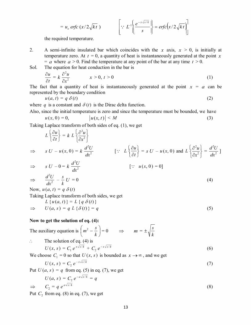
= ou )2/( tkxerfc

tkxerfcs

eLksx

2//

1

the required temperature. 2. A semi-infinite insulated bar which coincides with the x axis, x > 0, is initially at temperature zero. At t = 0, a quantity of heat is instantaneously generated at the point x = a where a > 0. Find the temperature at any point of the bar at any time t > 0. Sol. The equation for heat conduction in the bar is

tu

= k 2

2

xu

x > 0, t > 0 (1)

The fact that a quantity of heat is instantaneously generated at the point x = a can be represented by the boundary condition ),( tau = q )(t (2) where q is a constant and )(t is the Dirac delta function. Also, since the initial temperature is zero and since the temperature must be bounded, we have )0,(xu = 0, ),( txu < M (3) Taking Laplace transform of both sides of eq. (1), we get

L

tu = k L

2

2

xu

s U ‒ )0,(xu = k 2

2

dxUd [ L

tu = s U ‒ )0,(xu and L

2

2

xu = 2

2

dxUd ]

s U ‒ 0 = k 2

2

dxUd [ )0,(xu = 0]

2

2

dxUd ‒

ks U = 0 (4)

Now, ),( tau = q )(t Taking Laplace transform of both sides, we get L { ),( tau } = L { q )(t } ),( saU = q L { )(t } = q (5) Now to get the solution of eq. (4):

The auxiliary equation is

ksm2 = 0 m =

ks

The solution of eq. (4) is ),( sxU = 1C ksxe / + 2C ksxe / (6) We choose 1C = 0 so that ),( sxU is bounded as x , and we get

),( sxU = 2C ksxe / (7) Put ),( saU = q from eq. (5) in eq. (7), we get

),( saU = 2C ksae / = q

2C = q ksae / (8) Put 2C from eq. (8) in eq. (7), we get

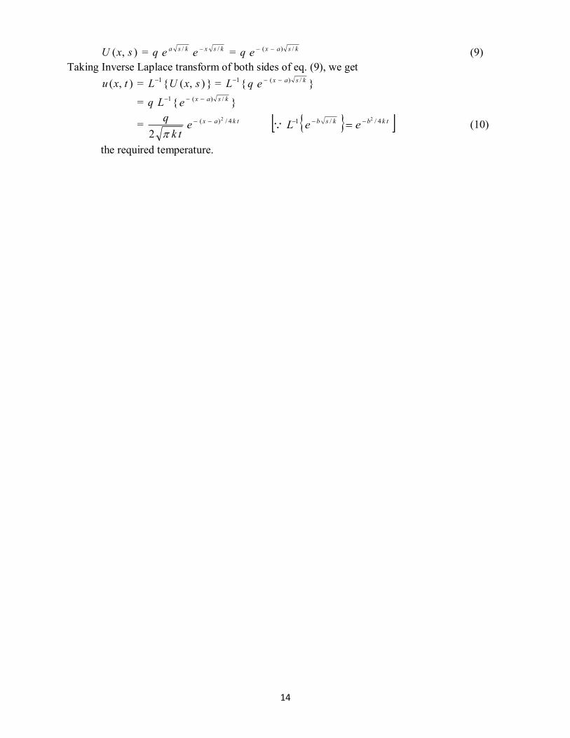
14

),( sxU = q ksae / ksxe / = q ksaxe /)( (9) Taking Inverse Laplace transform of both sides of eq. (9), we get ),( txu = 1L { ),( sxU } = 1L { q ksaxe /)( }

= q 1L { ksaxe /)( }

= tk

q2

tkaxe 4/)( 2 tkbksb eeL 4//1 2 (10)

the required temperature.

Documents

Lecture : 3 (APPLICATIONS OF LAPLACE TRANSFORMS)...Lecture : 3 (APPLICATIONS OF LAPLACE TRANSFORMS) Course : B.Sc. (H) Physics Semester : IV Subject : Mathematical Physics III UPC