Lecture 15: Effect modification, and confounding in ...eckel/biostat2/slides/lecture15.pdfLecture 15: Effect modification, and confounding in logistic regression Sandy Eckel [email protected]

1

Lecture 15: Effect modification, and confounding in logistic regression

Sandy [email protected]

16 May 2008

2

Today’s logistic regression topics

� Including categorical predictor

� create dummy/indicator variables

� just like for linear regression

� Comparing nested models that differ by two or more variables for logistic regression

� Chi-square (X2) Test of Deviance

� i.e., likelihood ratio test

� analogous to the F-test for nested models in linear regression

� Effect Modification and Confounding

3

Example

� Mean SAT scores were compared for the 50 US states. The goal of the study was to compare overall SAT scores using state-wide predictors such as

� per-pupil expenditures

� average teachers’ salary

4

Variables

� Outcome� Total SAT score [sat_low]

� 1=low, 0=high

� Primary predictor� Average expenditures per pupil [expen] in thousands

� Continuous, range: 3.65-9.77, mean: 5.9

� Doesn’t include 0: center at $5,000 per pupil

� Secondary predictor� Mean teacher salary in thousands, in quartiles

� salary1 – lowest quartile

� salary2 – 2nd quartile

� salary3 – 3rd quartile

� salary4 – highest quartile

� four dummy variables for four categories; must exclude one category to create a reference group

5

Analysis Plan

� Assess primary relationship (parent model)

� Add secondary predictor in separate model (extended model)

� Determine if secondary predictor is statistically significant

� How? Use the Chi-square test of deviance

6

Models and Results (note that only exponentiated slopes are shown)

Model 1 (Parent): Only primary predictor------------------------------------------------------------------------------

sat_low | Odds Ratio Std. Err. z P>|z| [95% Conf. Interval]

-------------+----------------------------------------------------------------

expenc | 2.484706 .8246782 2.74 0.006 1.296462 4.76201

------------------------------------------------------------------------------

Model 2 (Extended): Primary Predictor and Secondary Predictor------------------------------------------------------------------------------

sat_low | Odds Ratio Std. Err. z P>|z| [95% Conf. Interval]

-------------+----------------------------------------------------------------

expenc | 1.796861 .7982988 1.32 0.187 .7522251 4.292213

salary2 | 2.783137 2.815949 1.01 0.312 .3830872 20.21955

salary3 | 2.923654 3.2716 0.96 0.338 .326154 26.20773

salary4 | 4.362678 6.147015 1.05 0.296 .2756828 69.03933

------------------------------------------------------------------------------

( ) 5ββ1

log 10 −+=

−eExpenditur

p

p

)4(β)3(β)2(β)5(ββ1

log 43210 =+=+=+−+=

−SalaryISalaryISalaryIeExpenditur

p

p

7

The X2 Test of Deviance

� We want to compare the parent model to an extended model, which differs by the three dummy variables for the four salary quartiles.

� The X2 test of deviance compares nested logistic regression models� We use it for nested models that differ by two or more variables because the Wald test cannot be used in that situation

8

Performing the Chi-square test of deviance for nested logistic regression

1. Get the log likelihood (LL) from both models� Parent model: LL = -28.94

� Extended model: LL = -28.25

2. Find the deviance for both models

� Deviance = -2(log likelihood)

� Parent model: Deviance = -2(-28.94) = 57.88

� Extended model: Deviance = -2(-28.25) = 56.50

� Deviance is analogous to residual sums of squares (RSS) in linear regression; it measures the ‘deviation’still available in the model

� A saturated model is one in which every Y is perfectly predicted

9

Performing the Chi-square test of deviance for nested logistic regression, cont…

3. Find the change in deviance between the nested models

= devianceparent – devianceextended= 57.88 - 56.50= 1.38 = Test Statistic (X2)

4. Evaluate the change in deviance� The change in deviance is an observed Chi-square statistic

� df = # of variables added

� H0: all new β’s are 0 in the populationi.e., H0: the parent model is better

10

The Chi-square test of deviance for our nested logistic regression example

� H0: After adjusting for per-pupil expenditures, all the slopes on salary indicators are 0 (β2= β3= β4= 0 )

� X2obs = 1.38

� df = 3

� With 3 df and α=0.05, X2cr is 7.81

� X2obs < X2cr

� Fail to reject H0� Conclude: After adjusting for per-pupil expenditure, teachers’ salary is not a statistically significant predictor of low SAT scores

11

Notes about Chi-square deviance test

� The deviance test gives us a frameworkin which to add several predictors to a model simultaneously

� Can only handle nested models

� Analogous to F-test for linear regression

� Also known as "likelihood ratio test"

12

1. Fit parent modelfit.parent <- glm(y~x1, family=binomial())

2. Fit the extended model (parent model is nested within the extended model)fit.extended <- glm(y~x1+x2+x3, family=binomial())

3. Perform the Chi-square deviance testanova(fit.parent, fit.extended, test="Chi")

Example output:Analysis of Deviance Table

Model 1: y ~ x1

Model 2: y ~ x1 + x2 + x3

Resid. Df Resid. Dev Df Deviance P(>|Chi|)

1 48 64.250

2 46 48.821 2 15.429 0.0004464

How can I do the Chi-square deviance test in R?

Chi-square Test Statistic

Degrees of freedom

P-value

13

Effect Modification and Confoundingin Logistic Regression

Heart Disease

Smoking and Coffee

Example

14

Effect modification in logistic regression

� Just like with linear regression, we may wantto allow different relationships between the primary predictor and outcome across levelsof another covariate

� We can model such relationships by fittinginteraction terms in logistic regressions

� Modelling effect modification will requiredealing with two or more covariates

15

Logistic models with two covariates

� logit(p) = ββββ0 + ββββ1X1 + ββββ2X2

Then:

logit(p | X1=X1+1,X2=X2) = β0+ β1(X1+1)+ β2X2logit(p | X1=X1 ,X2=X2) = β0+ β1(X1 )+ β2X2

∆ in log-odds = β1

� ββββ1 is the change in log-odds for a 1 unit change in X1 provided X2 is held constant.

16

Interpretation in General

� Also: log = β1

� And: OR = exp(ββββ1) !!

� exp(β1) is the multiplicative change in odds for a 1 unit increase in X1 provided X2 is held constant.

� The result is similar for X2

� What if the effects of each of X1and X2depend on the presence of the other?� Effect modification!

=

+=

)2

X,1

X|1odds(Y

)2

X1,1

X|1odds(Y

17

Data: Coronary Heart Disease (CHD),Smoking and Coffee

n = 151

18

Study Information

� Study Facts:

� Case-Control study (disease = CHD)

� 40-50 year-old males previously in good health

� Study questions:

� Is smoking and/or coffee related to an increased odds of CHD?

� Is the association of coffee with CHD higher among smokers? That is, is smoking an effect modifier of the coffee-CHD associations?

19

Fraction with CHD by smoking and coffee

Number in each cell is the proportion of the total number of individuals with that smoking/coffee combination that have CHD

20

Pooled data (ignoring smoking)

Odds ratio of CHD comparing coffee to non-coffee drinkers

95% CI = (1.14, 4.24)

2.2)34.1/(34.

)53.1/(53.=

−

−

21

Among Non-Smokers


95% CI = (0.82, 4.9)

06.2)26.1/(26.

)42.1/(42.=

−

−

P(CHD| Coffee drinker) = 15/(15+21) = 0.42

P(CHD| Not Coffee drinker) = 15/(15+42) = 0.26

22

Among Smokers


95% CI = (0.42, 4.0)

29.1)58.1/(58.

)64.1/(64.=

−

−

P(CHD| Coffee drinker) = 25/(25+14) = 0.64

P(CHD| Not Coffee drinker) = 11/(11+8) = 0.58

23

Plot Odds Ratios and 95% CIs

24

Define Variables

� Yi = 1 if CHD case, 0 if control

� coffeei = 1 if Coffee Drinker, 0 if not

� smokei = 1 if Smoker, 0 if not

� pi = Pr (Yi = 1)

� ni = Number observed at patterni of Xs

25

Logistic Regression Model

� Yi are independent

� Random partYi are from a Binomial (ni, pi) distribution

� Systematic partlog odds (Yi=1) (or logit( Yi=1) ) is a function of

� Coffee

� Smoking

� and coffee-smoking interaction

iiii

i

i smokecoffeesmokecoffeep

p×+++=

−3210

1log ββββ

26

Interpretations – stratify by smoking status

If smoke = 0

If smoke = 1

� exp(β1): odds ratio of being a CHD case for coffee drinkers -vs- non-drinkers among non-smokers

� exp(β1+β3): odds ratio of being a CHD case for coffee drinkers -vs- non-drinkers among smokers

iiii

i


p×+++=

−3210

1log ββββ

i

i

i coffeep

p10

1log ββ +=

−

iii

i

i coffeecoffeecoffeep

p)()(11

1log 31203210 ββββββββ +++=×+×++=

−

27

Interpretations – stratify by coffee drinking

If coffee = 0

If coffee = 1

� exp(β2): odds ratio of being a CHD case for smokers -vs- non-smokers among non-coffee drinkers

� exp(β2+β3): odds ratio of being a CHD case for smokers -vs- non-smokers among coffee drinkers

iiii

i


p×+++=

−3210

1log ββββ

i

i

i smokep

p20

1log ββ +=

−

iii

i

i smokesmokesmokep

p)()(11

1log 32103210 ββββββββ +++=×++×+=

−

28

Interpretations

� Probability of CHD if all X’s are zero

� i.e., fraction of cases among non- smoking non-coffee drinking individuals in the sample (determined by sampling plan)

� exp(β3): ratio of odds ratios

What do we mean by this?

0

0

1β

β

e

e

+

iiii

i


p×+++=

−3210

1log ββββ

29

exp(β3) Interpretations

� exp(β3): factor by which odds ratio of being a CHD case for coffee drinkers -vs- nondrinkers is multiplied for smokers as compared to non-smokers

or� exp(β3): factor by which odds ratio of being a CHD case for smokers -vs- non-smokers is multiplied for coffee drinkers as compared to non-coffee drinkers

COMMON IDEA: Additional multiplicative change in the odds ratio beyond the smoking or coffee drinking effect alone when you have both of these risk factors present

iiii

i


p×+++=

−3210

1log ββββ

30

Some Special Cases:No smoking or coffee drinking effects

� Given

� If β1 = β2 = β3 = 0

� Neither smoking nor coffee drinking is associated with increased risk of CHD

iiii

i


p×+++=

−3210

1log ββββ

31

Some Special Cases:Only one effect

� Given

� If β2 = β3 = 0

� Coffee drinking, but not smoking, is associated with increased risk of CHD

� If β1 = β3 = 0

� Smoking, but not coffee drinking, is associated with increased risk of CHD

iiii

i


p×+++=

−3210

1log ββββ

32

Some Special Cases

� If β3 = 0

� Smoking and coffee drinking are both associated with risk of CHD but the odds ratio of CHD-smoking is the same at both levels of coffee

� Smoking and coffee drinking are both associated with risk of CHD but the odds ratio of CHD-coffee is the same at both levels of smoking

� Common idea: the effects of each of these risk factors is purely additive (on the log-odds scale), there is no interaction

iiii

i


p×+++=

−3210

1log ββββ

33

Model 1: main effect of coffee

Logit estimates Number of obs = 151

LR chi2(1) = 5.65

Prob > chi2 = 0.0175

Log likelihood = -100.64332 Pseudo R2 = 0.0273

------------------------------------------------------------------------------

chd | Coef. Std. Err. z P>|z| [95% Conf. Interval]

-------------+----------------------------------------------------------------

coffee | .7874579 .3347123 2.35 0.019 .1314338 1.443482

(Intercept) | -.6539265 .2417869 -2.70 0.007 -1.12782 -.1800329

------------------------------------------------------------------------------

i

i

i coffeep

p10

1log ββ +=

−

34

Model 2: main effects of coffee and smoke


LR chi2(2) = 15.19

Prob > chi2 = 0.0005


------------------------------------------------------------------------------


-------------+----------------------------------------------------------------

coffee | .5269764 .3541932 1.49 0.137 -.1672295 1.221182

smoke | 1.101978 .3609954 3.05 0.002 .3944404 1.809516

(Intercept) | -.9572328 .2703086 -3.54 0.000 -1.487028 -.4274377

------------------------------------------------------------------------------

ii

i

i smokecoffeep

p210

1log βββ ++=

−

35

Model 3: main effects of coffee and smoke AND their interaction


LR chi2(3) = 15.55

Prob > chi2 = 0.0014


------------------------------------------------------------------------------


-------------+----------------------------------------------------------------

coffee | .6931472 .4525062 1.53 0.126 -.1937487 1.580043

smoke | 1.348073 .5535208 2.44 0.015 .2631923 2.432954

coffee_smoke | -.4317824 .7294515 -0.59 0.554 -1.861481 .9979163

(Intercept)| -1.029619 .3007926 -3.42 0.001 -1.619162 -.4400768

------------------------------------------------------------------------------

iiii

i


p×+++=

−3210

1log ββββ

36

Comparing Models 1 & 2Question: Is smoking a confounder?

Model1

Model 2

-3.5.27-.96Intercept

1.5.35.53Coffee

3.1.361.10Smoking

2.4.33.79Coffee

-2.7.24-.65Intercept

zseEstVariable

37

Look at Confidence Intervals

� Without Smoking

OR = e0.79 = 2.2� 95% CI for log(OR): 0.79 ± 1.96(0.33)

= (0.13, 1.44)

� 95% CI for OR: (e0.13, e1.44)

= (1.14, 4.24)

� With Smoking (adjusting for smoking)

OR = e0.53 = 1.7

� Smoking does not confound the relationship between coffee drinking and CHD � since 1.7 is in the 95% CI from the model without smoking

38

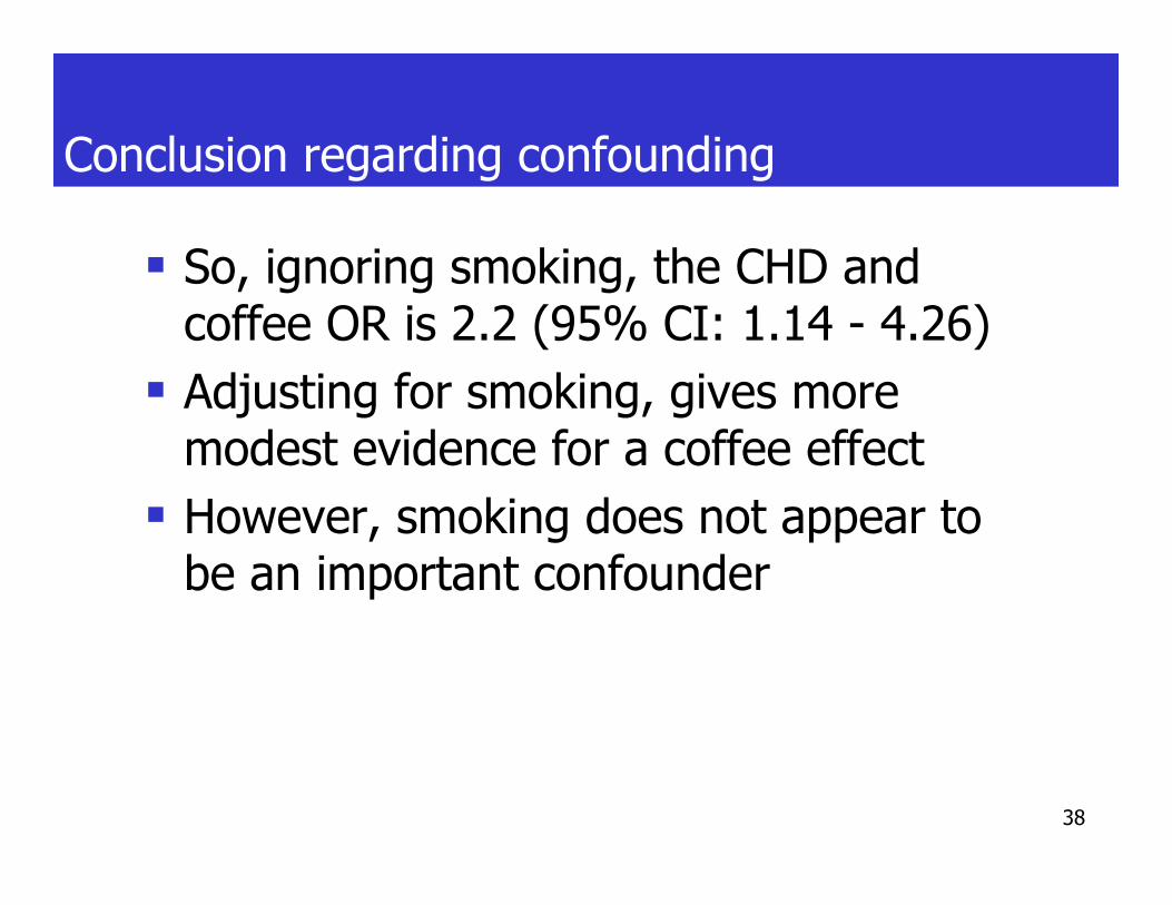
Conclusion regarding confounding

� So, ignoring smoking, the CHD and coffee OR is 2.2 (95% CI: 1.14 - 4.26)

� Adjusting for smoking, gives more modest evidence for a coffee effect

� However, smoking does not appear to be an important confounder

39

Interaction ModelQuestion: Is smoking an effect modifier of CHD-coffee association?

Model 3

2.4.551.3Smoking

-.59.73-.43Coffee*Smoking

1.5.45.69Coffee

-3.4.30-1.0Intercept

zseEstVariable

40

Testing Interaction Term

� Z= -0.59, p-value = 0.554

� We fail to reject H0: interaction slope= 0

� And we conclude there is little evidence that smoking is an effect modifier!

41

Question: Model selection

What model should we choose to describe the relationship of coffee

and smoking with CHD?

42

Fitted Values� We can use transform to get fitted probabilities and compare with observed proportions using each of the three models

� Model 1:

� Model 2:

� Model 3:

.79Coffee.65-

e1

eˆ

.79Coffee-.65

+

+=

+

p

1.1Smoking.53Coffee.96-

e1

eˆ

1.1Smoking.53Coffee-.96

++

+=

++

p

Smoking)*.43(Coffee-1.3Smoking.69Coffee.1.03-

e1

eˆ

Smoking)*.43(Coffee-1.3Smoking.69Coffee-.1.03

++

+=

++

p

43

Observed vs Fitted Values

44

Saturated Model

� Note that fitted values from Model 3 exactly match the observed values indicating a “saturated” model that gives perfect predictions

� Although the saturated model will always result in a perfect fit, it is usually not the best model (e.g., when there are continuous covariates or many covariates)

45

Likelihood Ratio Test

� The Likelihood Ratio Test will help decide whether or not additional term(s) “significantly” improve the model fit

� Likelihood Ratio Test (LRT) statistic for comparing nested models is � -2 times the difference between the log likelihoods (LLs) for the Null -vs- Extended models

� We’ve already done this earlier in today’s lecture!!� Chi-square (X2) Test of Deviance is the same thing as the Likelihood Ratio Test

� Used to compare any pair of nested logistic regression models and get a p-value associated with the H0: the ‘new’ β’s all=0

46

Example summary write-up

� A case-control study was conducted with 151 subjects, 66 (44%) of whom had CHD, to assess the relative importance of smoking and coffee drinking as risk factors. The observed fractions of CHD cases by smoking, coffee strata are

47

Example Summary: Unadjusted ORs

� The odds of CHD was estimated to be 3.4 times higher among smokers compared to non-smokers � 95% CI: (1.7, 7.9)

� The odds of CHD was estimated to be 2.2 times higher among coffee drinkers compared to non-coffee drinkers � 95% CI: (1.1, 4.3)

48

Example Summary: Adjusted ORs

� Controlling for the potential confounding of smoking, the coffee odds ratio was estimated to be 1.7 with 95% CI: (.85, 3.4).

� Hence, the evidence in these data are insufficient to conclude coffee has an independent effect on CHD beyond that of smoking.

49

Example Summary: effect modification

� Finally, we estimated the coffee odds ratio separately for smokers and non-smokers to assess whether smoking is an effect modifier of the coffee-CHD relationship. For the smokers and non-smokers, the coffee odds ratio was estimated to be 1.3 (95% CI: .42, 4.0) and 2.0 (95% CI: .82, 4.9) respectively. There is little evidence of effect modification in these data.

50

Summary of Lecture 15

� Including categorical predictors in logisiticregression� create dummy/indicator variables� just like for linear regression

� Comparing nested models that differ by two or more variables for logistic regression� Chi-square (X2) Test of Deviance

� i.e., likelihood ratio test

� analogous to the F-test for nested models in linear regression

� Effect Modification and Confounding in logistic regression

Documents

Lecture 15: Effect modification, and confounding in ...eckel/biostat2/slides/lecture15.pdfLecture 15: Effect modification, and confounding in logistic regression Sandy Eckel [email protected]