NRMT 2270, Photogrammetry/Remote Sensing

Lecture 11

Calculating the Number of Photos and Flight Lines in a Photo Project

LiDAR, RADAR

Tomislav Sapic GIS Technologist

Faculty of Natural Resources Management Lakehead University

Scale vs. GSD

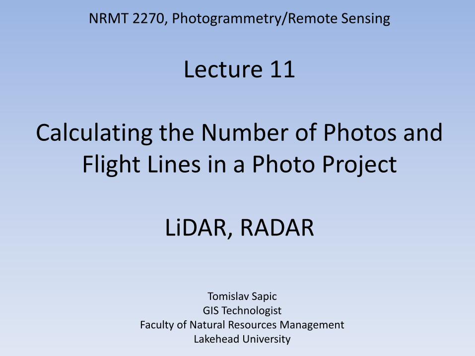
• Ground sampling distance (GSD) of an image states the width of the ground represented by an image cell (pixel).

• The concept of scale has been traditionally applied to hard copy photos and maps.

• Because of easy zooming in and out of digital images in a digital, GIS, environment, and because of easy printout enlargement the concept of scale does not fit well digital images -- GSD (spatial resolution) is preferred.

• Rather than asking “At what scale should I fly this digital imagery?,” one today asks “At what GSD should I fly this digital imagery?”

• But when it comes to calculating the number of photos required to cover an area and the frequency of taking them during the flight so that a targeted end overlap (i.e., ~60%) is achieved, then scale becomes useful again.

Calculate the Number of Photos for a Flight Project

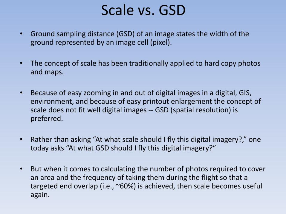
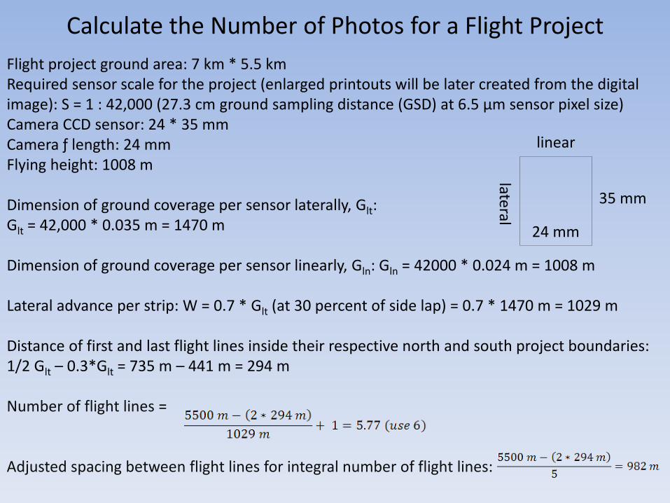
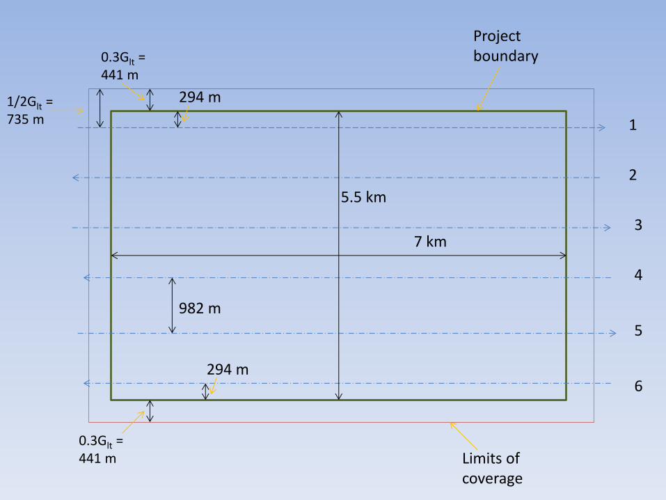
Flight project ground area: 7 km * 5.5 km Required sensor scale for the project (enlarged printouts will be later created from the digital image): S = 1 : 42,000 (27.3 cm ground sampling distance (GSD) at 6.5 μm sensor pixel size) Camera CCD sensor: 24 * 35 mm Camera ƒ length: 24 mm Flying height: 1008 m Dimension of ground coverage per sensor laterally, Glt: Glt = 42,000 * 0.035 m = 1470 m Dimension of ground coverage per sensor linearly, Gln: Gln = 42000 * 0.024 m = 1008 m Lateral advance per strip: W = 0.7 * Glt (at 30 percent of side lap) = 0.7 * 1470 m = 1029 m Distance of first and last flight lines inside their respective north and south project boundaries: 1/2 Glt – 0.3*Glt = 735 m – 441 m = 294 m Number of flight lines =

Adjusted spacing between flight lines for integral number of flight lines:

24 mm

35 mm

lateral

linear

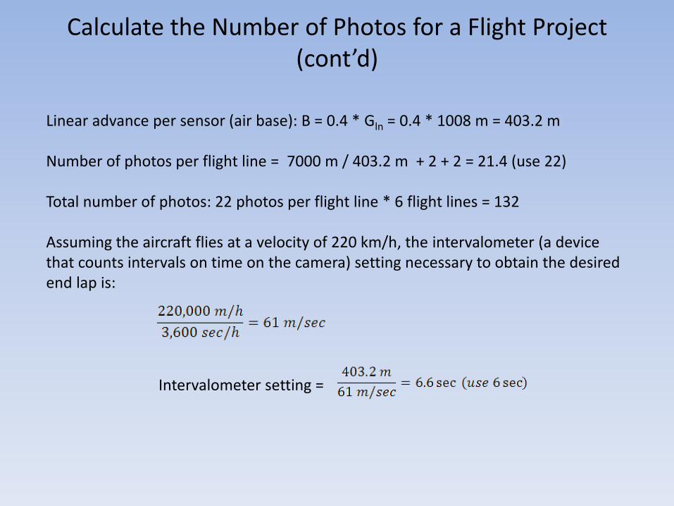
Calculate the Number of Photos for a Flight Project (cont’d)

Linear advance per sensor (air base): B = 0.4 * Gln = 0.4 * 1008 m = 403.2 m Number of photos per flight line = 7000 m / 403.2 m + 2 + 2 = 21.4 (use 22) Total number of photos: 22 photos per flight line * 6 flight lines = 132 Assuming the aircraft flies at a velocity of 220 km/h, the intervalometer (a device that counts intervals on time on the camera) setting necessary to obtain the desired end lap is:

Intervalometer setting =

1

2

3

4

5

6

7 km

5.5 km

1/2Glt = 735 m

0.3Glt = 441 m

294 m

294 m

0.3Glt = 441 m

982 m

Project boundary

Limits of coverage

Active Remote Sensing Systems

• Photo cameras are passive remote sensing systems – the recorded energy is produced by the sun and captured by the remote sensing system (camera).

• As opposed to passive remote sensing systems, active remote sensing systems both produce (emit) and record energy.

• Two of such systems are LiDAR, which is rapidly and increasingly applied in forest and natural resources related sciences and economical sectors, and RADAR, which is applied to a lesser degree.

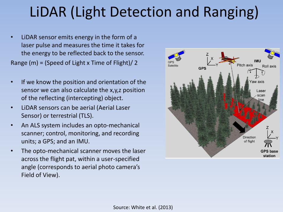
LiDAR (Light Detection and Ranging)

• LiDAR sensor emits energy in the form of a laser pulse and measures the time it takes for the energy to be reflected back to the sensor.

Range (m) = (Speed of Light x Time of Flight)/ 2

• If we know the position and orientation of the sensor we can also calculate the x,y,z position of the reflecting (intercepting) object.

• LiDAR sensors can be aerial (Aerial Laser Sensor) or terrestrial (TLS).

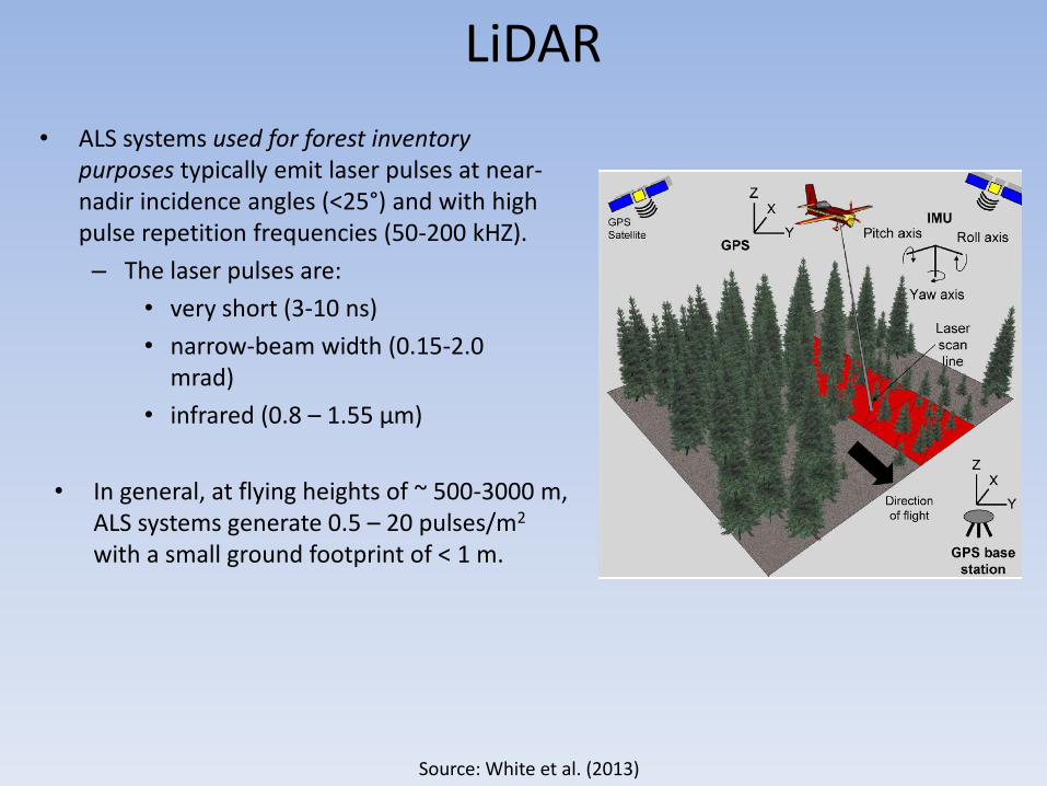
• An ALS system includes an opto-mechanical scanner; control, monitoring, and recording units; a GPS; and an IMU.

• The opto-mechanical scanner moves the laser across the flight pat, within a user-specified angle (corresponds to aerial photo camera’s Field of View).

Source: White et al. (2013)

LiDAR

• ALS systems used for forest inventory purposes typically emit laser pulses at near-nadir incidence angles (<25°) and with high pulse repetition frequencies (50-200 kHZ).

– The laser pulses are:

• very short (3-10 ns)

• narrow-beam width (0.15-2.0 mrad)

• infrared (0.8 – 1.55 µm)

Source: White et al. (2013)

• In general, at flying heights of ~ 500-3000 m, ALS systems generate 0.5 – 20 pulses/m2

with a small ground footprint of < 1 m.

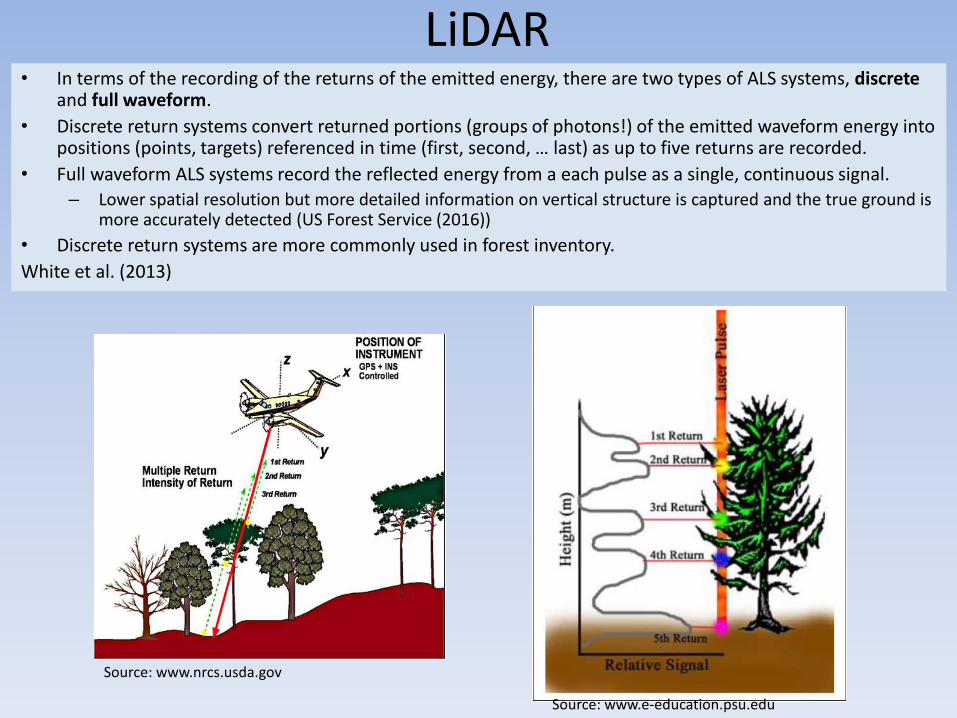
LiDAR • In terms of the recording of the returns of the emitted energy, there are two types of ALS systems, discrete

and full waveform.

• Discrete return systems convert returned portions (groups of photons!) of the emitted waveform energy into positions (points, targets) referenced in time (first, second, … last) as up to five returns are recorded.

• Full waveform ALS systems record the reflected energy from a each pulse as a single, continuous signal. – Lower spatial resolution but more detailed information on vertical structure is captured and the true ground is

more accurately detected (US Forest Service (2016))

• Discrete return systems are more commonly used in forest inventory.

White et al. (2013)

Source: www.nrcs.usda.gov

Source: www.e-education.psu.edu

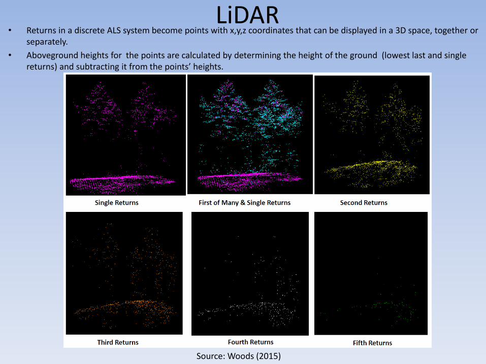
LiDAR • Returns in a discrete ALS system become points with x,y,z coordinates that can be displayed in a 3D space, together or

separately.

• Aboveground heights for the points are calculated by determining the height of the ground (lowest last and single returns) and subtracting it from the points’ heights.

Source: Woods (2015)

ALS data are used to:

• Measure tree height, tree density, stand basal area, forest biomass, forest volume.

• Measure and describe forest structure.

• Estimate wood fuel volumes.

• Create DEMs

LiDAR

Source: White et al. (2013)

Source: Treitz et al. (2016)

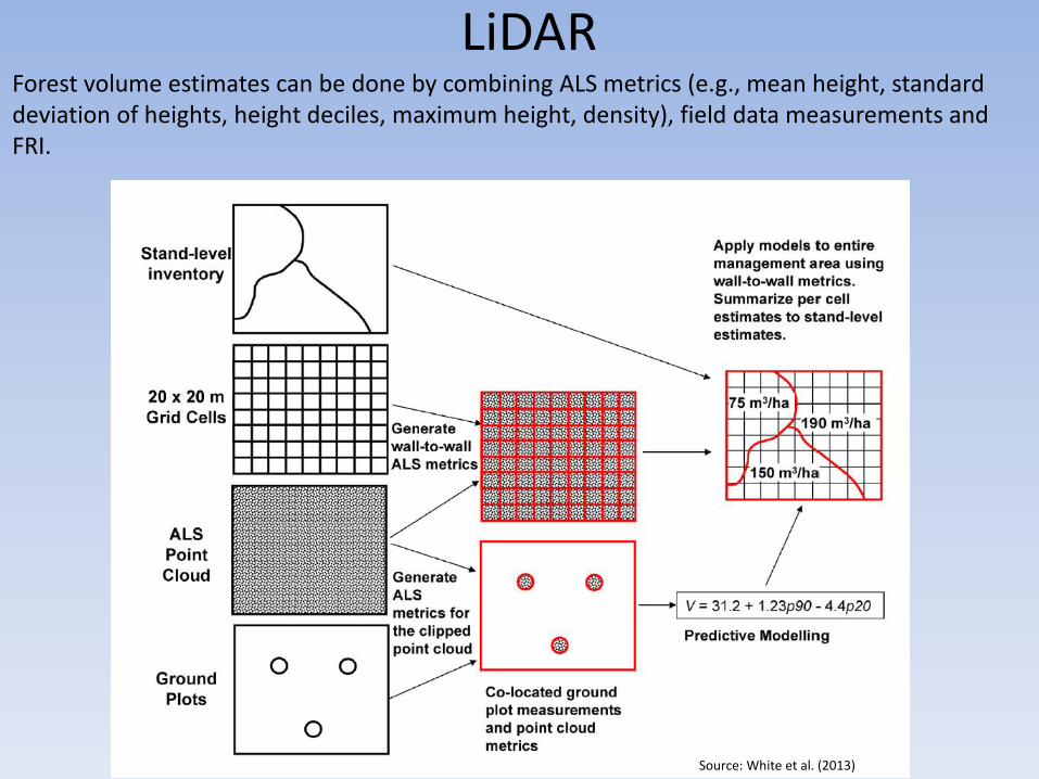
LiDAR Forest volume estimates can be done by combining ALS metrics (e.g., mean height, standard deviation of heights, height deciles, maximum height, density), field data measurements and FRI.

Source: White et al. (2013)

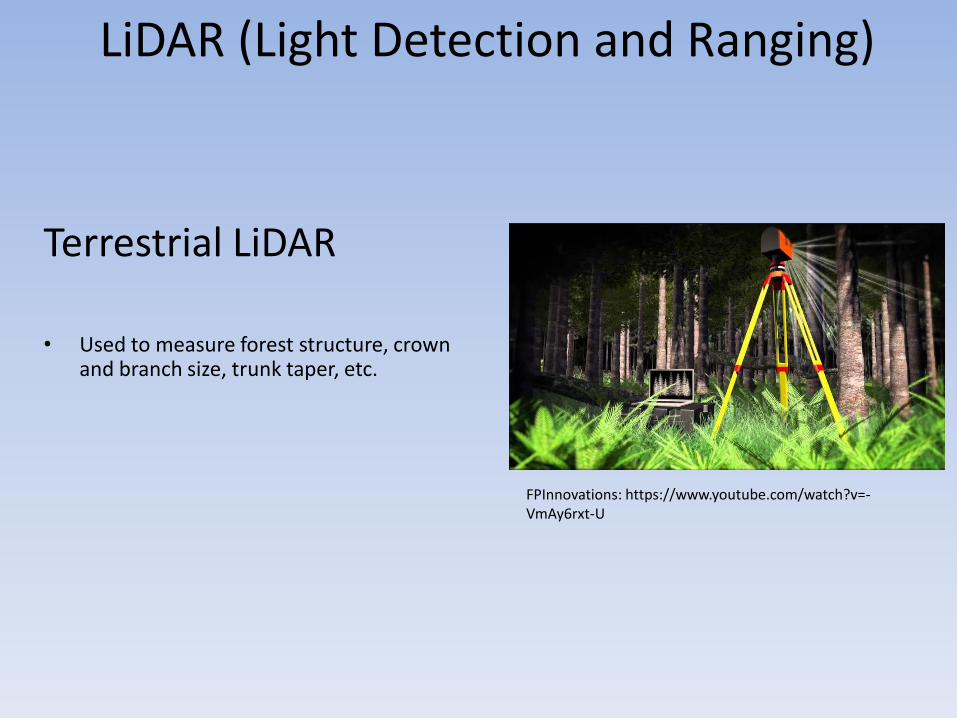
Terrestrial LiDAR

• Used to measure forest structure, crown and branch size, trunk taper, etc.

LiDAR (Light Detection and Ranging)

FPInnovations: https://www.youtube.com/watch?v=-VmAy6rxt-U

RADAR (Radio Detection And Ranging)

Source: NRC (2016)

• Similar to LiDAR, in a radar system, the transmitter generates short pulses of energy, in this case microwave (from just under a mm to 1 m em wavelength), at regular intervals which are focused by the antenna into a beam.

• The radar beams are sent at an oblique angle and the receiver antenna receives a portion of the transmitted energy reflected (backscattered “echo”).

• By measuring the time delay between the transmission and reception the distance “range’ to the objects is calculated.

NRC (2016).

Some of the major applications of radar are: • Forest structure measurement. • Flood and wetland mapping. • Soil moisture mapping. • Ice structure and type. NRC (2016).

An advantage of radar compared to LiDAR and aerial photography, is that radar beams pass through clouds because of the relatively long em waves.

References: Natural Resources Canada (NRC). 2016. Radar Basics. http://www.nrcan.gc.ca/earth-sciences/geomatics/satellite-imagery-air-photos/satellite-imagery-products/educational-resources/9355 NRC (2016). Viewed March 2016. Treitz P., M. Woods, K. Lim, V. Thomas, H. McCaughey. 2016. LiDAR remote sensing for natural resource management. http://www.queensu.ca/sbc/images/presentations/Treitz_P.pdf Viewed March 2016. US Forest Service. 2016. Introduction to LiDAR. http://www.fs.fed.us/eng/rsac/lidar_training/Introduction_to_Lidar/player.html . Viewed March 2016. White, J. C. , M. A. Wulder, A. Varhola, M. Vastaranta, N. C. Coops, B. D. Cook, D. Pitt, and M. Woods. 2013. A best practices guide for generating forest inventory attributes from airborne laser scanning data using an area-based approach. Natural Resources Canada, Canadian Forest Service, Canadian Wood Fibre Centre. Woods, M. 2015. Introduction to cloud points. Developing area-based forest inventories using LiDAR or photogrammetric point clouds and the LTK software workshop. Thunder Bay, Nov 25, 2015.