Embed Size (px)
Citation preview
Learning from Corrupted Binary Labels via Class-Probability Estimation (FullVersion)
Aditya Krishna Menon∗ [email protected] van Rooyen† [email protected] Soon Ong∗ [email protected] C. Williamson∗ [email protected]∗ National ICT Australia and The Australian National University, Canberra† The Australian National University and National ICT Australia, Canberra
AbstractMany supervised learning problems involvelearning from samples whose labels are cor-rupted in some way. For example, each labelmay be flipped with some constant probability(learning with label noise), or one may have apool of unlabelled samples in lieu of negativesamples (learning from positive and unlabelleddata). This paper uses class-probability estima-tion to study these and other corruption processesbelonging to the mutually contaminated distribu-tions framework (Scott et al., 2013), with threeconclusions. First, one can optimise balanced er-ror and AUC without knowledge of the corrup-tion parameters. Second, given estimates of thecorruption parameters, one can minimise a rangeof classification risks. Third, one can estimatecorruption parameters via a class-probability es-timator (e.g. kernel logistic regression) trainedsolely on corrupted data. Experiments on labelnoise tasks corroborate our analysis.
1. Learning from corrupted binary labelsIn many practical scenarios involving learning from binarylabels, one observes samples whose labels are corruptedversions of the actual ground truth. For example, in learn-ing from class-conditional label noise (CCN learning), thelabels are flipped with some constant probability (Angluin& Laird, 1988). In positive and unlabelled learning (PUlearning), we have access to some positive samples, but inlieu of negative samples only have a pool of samples whoselabel is unknown (Denis, 1998). More generally, suppose
Proceedings of the 32nd International Conference on MachineLearning, Lille, France, 2015. JMLR: W&CP volume 37. Copy-right 2015 by the author(s).
there is a notional clean distribution D over instances andlabels. We say a problem involves learning from corruptedbinary labels if we observe training samples drawn fromsome corrupted distribution Dcorr such that the observedlabels do not represent those we would observe under D.
A fundamental question is whether one can minimise agiven performance measure with respect to D, given ac-cess only to samples from Dcorr. Intuitively, in generalthis requires knowledge of the parameters of the corrup-tion process that determines Dcorr. This yields two fur-ther questions: are there measures for which knowledge ofthese corruption parameters is unnecessary, and for othermeasures, can we estimate these parameters?
In this paper, we consider corruption problems belonging tothe mutually contaminated distributions framework (Scottet al., 2013). We then study the above questions throughthe lens of class-probability estimation, with three conclu-sions. First, optimising balanced error (BER) as-is on cor-rupted data equivalently optimises BER on clean data, andsimilarly for the area under the ROC curve (AUC). Thatis, these measures can be optimised without knowledge ofthe corruption process parameters; further, we present evi-dence that these are essentially the only measures with thisproperty. Second, given estimates of the corruption param-eters, a range of classification measures can be minimisedby thresholding corrupted class-probabilities. Third, undersome assumptions, these corruption parameters may be es-timated from the range of the corrupted class-probabilities.
For all points above, observe that learning requires onlycorrupted data. Further, corrupted class-probability esti-mation can be seen as treating the observed samples as ifthey were uncorrupted. Thus, our analysis gives justifica-tion (under some assumptions) for this apparent heuristicin problems such as CCN and PU learning.
While some of our results are known for the special casesof CCN and PU learning, our interest is in determining to
Learning from Corrupted Binary Labels via Class-Probability Estimation
what extent they generalise to other label corruption prob-lems. This is a step towards a unified treatment of theseproblems. We now fix notation and formalise the problem.
2. Background and problem setupFix an instance space X. We denote byD some distributionover X × {±1}, with (X,Y) ∼ D a pair of random vari-ables. Any D may be expressed via the class-conditionaldistributions (P,Q) = (P(X | Y = 1),P(X | Y = −1))and base rate π = P(Y = 1), or equivalently via marginaldistribution M = P(X) and class-probability functionη : x 7→ P(Y = 1 | X = x). When referring to theseconstituent distributions, we write D as DP,Q,π or DM,η.
2.1. Classifiers, scorers, and risks
A classifier is any function f : X→ {±1}. A scorer is anyfunction s : X → R. Many learning methods (e.g. SVMs)output a scorer, from which a classifier is formed by thresh-olding about some t ∈ R. We denote the resulting classifierby thresh(s, t) : x 7→ sign(s(x)− t).
The false positive and false negative rates of a classifierf are denoted FPRD(f),FNRD(f), and are defined byP
X∼Q(f(X) = 1) and P
X∼P(f(X) = −1) respectively.
Given a function Ψ: [0, 1]3 → [0, 1], a classification per-formance measure ClassDΨ : {±1}X → [0, 1] assesses theperformance of a classifier f via (Narasimhan et al., 2014)
ClassDΨ(f) = Ψ(FPRD(f),FNRD(f), π).
A canonical example is the misclassification error, whereΨ: (u, v, p) 7→ p · v+ (1− p) · u. Given a scorer s, we useClassDΨ(s; t) to refer to ClassDΨ(thresh(s, t)).
The Ψ-classification regret of a classifier f : X→ {±1} is
regretDΨ(f) = ClassDΨ(f)− infg : X→{±1}
ClassDΨ(g).
A loss is any function ` : {±1} ×R→ R+. Given a distri-bution D, the `-risk of a scorer s is defined as
LD` (s) = E(X,Y)∼D
[`(Y, s(X))] . (1)
The `-regret of a scorer, regretD` , is as per the Ψ-regret.
We say ` is strictly proper composite (Reid & Williamson,2010) if argmins LD` (s) is some strictly monotone trans-formation ψ of η, i.e. we can recover class-probabilitiesfrom the optimal prediction via the link function ψ. We callclass-probability estimation (CPE) the task of minimisingEquation 1 for some strictly proper composite `.
The conditional Bayes-risk of a strictly proper composite` is L` : η 7→ η`1(ψ(η)) + (1 − η)`−1(ψ(η)). We call
Quantity Clean Corrupted
Joint distribution D Corr(D,α, β, πcorr)or Dcorr
Class-conditionals P,Q Pcorr, Qcorr
Base rate π πcorr
Class-probability η ηcorr
Ψ-optimal threshold tDΨ tDcorr,Ψ
Table 1. Common quantities on clean and corrupted distributions.
` strongly proper composite with modulus λ if L` is λ-strongly concave (Agarwal, 2014). Canonical examples ofsuch losses are the logistic and exponential loss, as used inlogistic regression and AdaBoost respectively.
2.2. Learning from contaminated distributions
Suppose DP,Q,π is some “clean” distribution where per-formance will be assessed. (We do not assume thatD is separable.) In MC learning (Scott et al., 2013),we observe samples from some corrupted distributionCorr(D,α, β, πcorr) over X × {±1}, for some unknownnoise parameters α, β ∈ [0, 1] with α + β < 1; where theparameters are clear from context, we occasionally refer tothe corrupted distribution as Dcorr. The corrupted class-conditional distributions Pcorr, Qcorr are
Pcorr = (1− α) · P + α ·QQcorr = β · P + (1− β) ·Q,
(2)
and the corrupted base rate πcorr in general has no relationto the clean base rate π. (If α+β = 1, then Pcorr = Qcorr,making learning impossible, whereas if α+ β > 1, we canswap Pcorr, Qcorr.) Table 1 summarises common quantitieson the clean and corrupted distributions.
From (2), we see that none of Pcorr, Qcorr or πcorr con-tain any information about π in general. Thus, estimatingπ from Corr(D,α, β, πcorr) is impossible in general. Theparameters α, β are also non-identifiable, but can be esti-mated under some assumptions on D (Scott et al., 2013).
2.3. Special cases of MC learning
Two special cases of MC learning are notable. In learningfrom class-conditional label noise (CCN learning) (An-gluin & Laird, 1988), positive samples have labels flippedwith probability ρ+, and negative samples with probabilityρ−. This can be shown to reduce to MC learning with
α = π−1corr · (1− π) · ρ− , β = (1− πcorr)
−1 · π · ρ+, (3)
and the corrupted base rate πcorr = (1−ρ+)·π+ρ−·(1−π).(See Appendix C for details.)
Learning from Corrupted Binary Labels via Class-Probability Estimation
In learning from positive and unlabelled data (PU learn-ing) (Denis, 1998), one has access to unlabelled samples inlieu of negative samples. There are two subtly different set-tings: in the case-controlled setting (Ward et al., 2009), theunlabelled samples are drawn from the marginal distribu-tion M , corresponding to MC learning with α = 0, β = π,and πcorr arbitrary. In the censoring setting (Elkan & Noto,2008), observations are drawn from D followed by a labelcensoring procedure. This is in fact a special of CCN (andhence MC) learning with ρ− = 0.
3. BER and AUC are immune to corruptionWe first show that optimising balanced error and AUC oncorrupted data is equivalent to doing so on clean data.Thus, with a suitably rich function class, one can opti-mise balanced error and AUC from corrupted data withoutknowledge of the corruption process parameters.
3.1. BER minimisation is immune to label corruption
The balanced error (BER) (Brodersen et al., 2010) of aclassifier is simply the mean of the per-class error rates,
BERD(f) =FPRD(f) + FNRD(f)
2.
This is a popular measure in imbalanced learning problems(Cheng et al., 2002; Guyon et al., 2004) as it penalises sac-rificing accuracy on the rare class in favour of accuracy onthe dominant class. The negation of the BER is also knownas the AM (arithmetic mean) metric (Menon et al., 2013).
The BER-optimal classifier thresholds the class-probabilityfunction at the base rate (Menon et al., 2013), so that:
argminf : X→{±1}
BERD(f) = thresh(η, π) (4)
argminf : X→{±1}
BERDcorr(f) = thresh(ηcorr, πcorr), (5)
where ηcorr denotes the corrupted class-probability func-tion. As Equation 4 depends on π, it may appear that onemust know π to minimise the clean BER from corrupteddata. Surprisingly, the BER-optimal classifiers in Equa-tions 4 and 5 coincide. This is because of the followingrelationship between the clean and corrupted BER.
Proposition 1. Pick any D and Corr(D,α, β, πcorr).Then, for any classifier f : X→ {±1},
BERDcorr(f) = (1− α− β) · BERD(f) +α+ β
2, (6)
and so the minimisers of the two are identical.
Thus, when BER is the desired performance metric, we donot need to estimate the noise parameters, or the clean
base rate: we can (approximately) optimise the BER onthe corrupted data using estimates ηcorr, πcorr, from whichwe build a classifier thresh(ηcorr, πcorr). Observe that thisapproach effectively treats the corrupted samples as if theywere clean, e.g. in a PU learning problem, we treat the un-labelled samples as negative, and perform CPE as usual.
With a suitably rich function class, surrogate regret boundsquantify the efficacy of thresholding approximate class-probability estimates. Suppose we know the corrupted baserate1πcorr, and suppose that s is a scorer with low `-regreton the corrupted distribution for some proper compositeloss ` with link ψ i.e. ψ−1(s) is a good estimate of ηcorr.Then, the classifier resulting from thresholding this scorerwill attain low BER on the clean distribution D.
Proposition 2. Pick any D and Corr(D,α, β, πcorr). Let` be a strongly proper composite loss with modulus λ andlink function ψ. Then, for any scorer s : X→ R,
regretDBER(f) ≤ C(πcorr)
1− α− β·√
2
λ·√
regretDcorr
` (s),
where f = thresh(s, ψ(πcorr)) and C(πcorr) = (2 ·πcorr · (1− πcorr))
−1.
Thus, good estimates of the corrupted class-probabilitieslet us minimise the clean BER. Of course, learning fromcorrupted data comes at a price: compared to the regretbound obtained if we could minimise ` on the clean dis-tribution D, we have an extra penalty of (1 − α − β)−1.This matches our intuition that for high-noise regimes (i.e.α + β ≈ 1), we need more corrupted samples to learn ef-fectively with respect to the clean distribution; confer vanRooyen & Williamson (2015) for lower and upper boundson sample complexity for a range of corruption problems.
3.2. AUC maximisation is immune to label corruption
Another popular performance measure in imbalancedlearning scenarios is the area under the ROC curve (AUC).The AUC of a scorer, AUCD(s), is the probability of a ran-dom positive instance scoring higher than a random nega-tive instance (Agarwal et al., 2005):
EX∼P,X′∼Q
[Js(X) > s(X′)K +
1
2Js(X) = s(X′)K
].
We have a counterpart to Proposition 1 by rewriting theAUC as an average of BER across a range of thresholds((Flach et al., 2011); see Appendix A.5):
AUCD(s) =3
2− 2 · EX∼P [BERD(s; s(X))]. (7)
1Surrogate regret bounds may also be derived for an empiri-cally chosen threshold (Kotłowski & Dembczynski, 2015).
Learning from Corrupted Binary Labels via Class-Probability Estimation
Corollary 3. Pick any DP,Q,π and Corr(D,α, β, πcorr).Then, for any scorer s : X→ R,
AUCDcorr(s) = (1− α− β) ·AUCD(s) +α+ β
2. (8)
Thus, like the BER, optimising the AUC with respect tothe corrupted distribution optimises the AUC with respectto the clean one. Further, via recent bounds on the AUC-regret (Agarwal, 2014), we can show that a good corruptedclass-probability estimator will have good clean AUC.
Corollary 4. Pick any D and Corr(D,α, β, πcorr). Let `be a strongly proper composite loss with modulus λ. Then,for every scorer s : X→ R,
regretDAUC(s) ≤ C(πcorr)
1− α− β·√
2
λ·√
regretDcorr
` (s),
where C(πcorr) = (πcorr · (1− πcorr))−1.
What is special about the BER (and consequently the AUC)that lets us avoid estimation of the corruption parameters?To answer this, we more carefully study the structure ofηcorr to understand why Equation 4 and 5 coincide, andwhether any other measures have this property.
Relation to existing work For the special case of CCNlearning, Proposition 1 was shown in Blum & Mitchell(1998, Section 5), and for case-controlled PU learning, in(Lee & Liu, 2003; Zhang & Lee, 2008). None of theseworks established surrogate regret bounds.
4. Corrupted and clean class-probabilitiesThe equivalence between a specific thresholding of theclean and corrupted class-probabilities (Equations 4 and 5)hints at a relationship between the two functions. We nowmake this relationship explicit.
Proposition 5. For any DM,η and Corr(D,α, β, πcorr),
(∀x ∈ X) ηcorr(x) = T (α, β, π, πcorr, η(x)) (9)
where, for φ : z 7→ z1+z , T (α, β, π, πcorr, t) is given by
φ
(πcorr
1− πcorr·
(1− α) · 1−ππ ·
t1−t + α
β · 1−ππ ·
t1−t + (1− β)
). (10)
It is evident that ηcorr is a strictly monotone increasingtransform of η. This is useful to study classifiers basedon thresholding η, as per Equation 4. Suppose we wanta classifier of the form thresh(η, t). The structure ofηcorr means that this is equivalent to a corrupted classi-fier thresh(ηcorr, T (α, β, π, πcorr, t)), where the functionT (as per Equation 10) tells us how to modify the thresholdt on corrupted data. We now make this precise.
Corollary 6. Pick any DM,η and Corr(D,α, β, πcorr).Then, ∀x ∈ X and ∀t ∈ [0, 1],
η(x) > t ⇐⇒ ηcorr(x) > T (α, β, π, πcorr, t)
where T is as defined in Equation 10.
By viewing the minimisation of a general classificationmeasure in light of the above, we now return to the issueof why BER can avoid estimating corruption parameters.
Relation to existing work In PU learning, Proposition 5has been shown in both the case-controlled (McCullagh &Nelder, 1989, pg. 113), (Phillips et al., 2009; Ward et al.,2009) and censoring settings (Elkan & Noto, 2008, Lemma1). In CCN learning, Proposition 5 is used in Natarajanet al. (2013, Lemma 7). Corollary 6 is implicit in Scottet al. (2013, Proposition 1), but the explicit form for thecorrupted threshold is useful for subsequent analysis.
5. Classification from corrupted dataConsider the problem of optimising a classification mea-sure ClassDΨ(f) for some Ψ: [0, 1]3 → [0, 1]. For a rangeof Ψ, the optimal classifier is f = thresh(η, tDΨ) (Koyejoet al., 2014; Narasimhan et al., 2014), for some optimalthreshold tDΨ . For example, by Equation 4, the BER-optimal classifier thresholds class-probabilities at the baserate; other examples of such Ψ are those corresponding tomisclassification error, and the F-score. But by Corollary6, thresh(η, tDΨ) = thresh(ηcorr, t
Dcorr,Ψ), where
tDcorr,Ψ = T (α, β, π, πcorr, tDΨ) (11)
is the corresponding optimal corrupted threshold. Basedon this, we now look at two approaches to minimisingClassDΨ(f). For the purposes of description, we shall as-sume that α, β, π are known (or can be estimated). We thenstudy the practically important question of when these ap-proaches can be applied without knowledge of α, β, π.
5.1. Classification when tDΨ is known
Suppose that tDΨ has some closed-form expression; for ex-ample, for misclassification risk, tDΨ = 1/2. Then, thereis a simple strategy for minimising ClassDΨ : compute esti-mates ηcorr of the corrupted class probabilities, and thresh-old them via tDcorr,Ψ computed from Equation 11. Standardcost-sensitive regret bounds may then be invoked. For con-creteness, consider the misclassification risk, where plug-ging in tDΨ = 1/2 into Equation 10 gives
tDcorr,Ψ = φ
(πcorr
1− πcorr·
(1− α) · 1−ππ + α
β · 1−ππ + (1− β)
), (12)
for φ : z 7→ z/(1 + z). We have the following.
Learning from Corrupted Binary Labels via Class-Probability Estimation
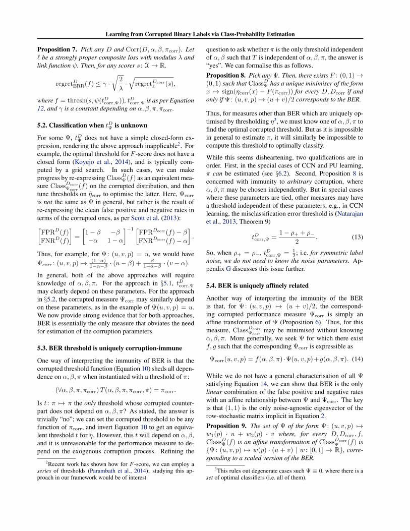
Proposition 7. Pick any D and Corr(D,α, β, πcorr). Let` be a strongly proper composite loss with modulus λ andlink function ψ. Then, for any scorer s : X→ R,
regretDERR(f) ≤ γ ·√
2
λ·√
regretDcorr
` (s),
where f = thresh(s, ψ(tDcorr,Ψ)), tDcorr,Ψ is as per Equation12, and γ is a constant depending on α, β, π, πcorr.
5.2. Classification when tDΨ is unknown
For some Ψ, tDΨ does not have a simple closed-form ex-pression, rendering the above approach inapplicable2. Forexample, the optimal threshold for F -score does not have aclosed form (Koyejo et al., 2014), and is typically com-puted by a grid search. In such cases, we can makeprogress by re-expressing ClassDΨ(f) as an equivalent mea-sure ClassDcorr
Ψcorr(f) on the corrupted distribution, and then
tune thresholds on ηcorr to optimise the latter. Here, Ψcorr
is not the same as Ψ in general, but rather is the result ofre-expressing the clean false positive and negative rates interms of the corrupted ones, as per Scott et al. (2013):[
FPRD(f)
FNRD(f)
]=
[1− β −β−α 1− α
]−1 [FPRDcorr(f)− βFNRDcorr(f)− α
].
Thus, for example, for Ψ: (u, v, p) = u, we would haveΨcorr : (u, v, p) 7→ (1−α)
1−α−β · (u− β) + β1−α−β · (v − α).
In general, both of the above approaches will requireknowledge of α, β, π. For the approach in §5.1, tDcorr,Ψ
may clearly depend on these parameters. For the approachin §5.2, the corrupted measure Ψcorr may similarly dependon these parameters, as in the example of Ψ(u, v, p) = u.We now provide strong evidence that for both approaches,BER is essentially the only measure that obviates the needfor estimation of the corruption parameters.
5.3. BER threshold is uniquely corruption-immune
One way of interpreting the immunity of BER is that thecorrupted threshold function (Equation 10) sheds all depen-dence on α, β, π when instantiated with a threshold of π:
(∀α, β, π, πcorr)T (α, β, π, πcorr, π) = πcorr.
Is t : π 7→ π the only threshold whose corrupted counter-part does not depend on α, β, π? As stated, the answer istrivially “no”; we can set the corrupted threshold to be anyfunction of πcorr, and invert Equation 10 to get an equiva-lent threshold t for η. However, this t will depend on α, β,and it is unreasonable for the performance measure to de-pend on the exogenous corruption process. Refining the
2Recent work has shown how for F -score, we can employ aseries of thresholds (Parambath et al., 2014); studying this ap-proach in our framework would be of interest.
question to ask whether π is the only threshold independentof α, β such that T is independent of α, β, π, the answer is“yes”. We can formalise this as follows.Proposition 8. Pick any Ψ. Then, there exists F : (0, 1)→(0, 1) such that ClassDΨ has a unique minimiser of the formx 7→ sign(ηcorr(x) − F (πcorr)) for every D,Dcorr if andonly if Ψ: (u, v, p) 7→ (u+ v)/2 corresponds to the BER.
Thus, for measures other than BER which are uniquely op-timised by thresholding η3, we must know one of α, β, π tofind the optimal corrupted threshold. But as it is impossiblein general to estimate π, it will similarly be impossible tocompute this threshold to optimally classify.
While this seems disheartening, two qualifications are inorder. First, in the special cases of CCN and PU learning,π can be estimated (see §6.2). Second, Proposition 8 isconcerned with immunity to arbitrary corruption, whereα, β, π may be chosen independently. But in special caseswhere these parameters are tied, other measures may havea threshold independent of these parameters; e.g., in CCNlearning, the misclassification error threshold is (Natarajanet al., 2013, Theorem 9)
tDcorr,Ψ =1− ρ+ + ρ−
2. (13)
So, when ρ+ = ρ−, tDcorr,Ψ = 12 ; i.e. for symmetric label
noise, we do not need to know the noise parameters. Ap-pendix G discusses this issue further.
5.4. BER is uniquely affinely related
Another way of interpreting the immunity of the BERis that, for Ψ: (u, v, p) 7→ (u + v)/2, the correspond-ing corrupted performance measure Ψcorr is simply anaffine transformation of Ψ (Proposition 6). Thus, for thismeasure, ClassDcorr
Ψcorrmay be minimised without knowing
α, β, π. More generally, we seek Ψ for which there existf, g such that the corresponding Ψcorr is expressible as
Ψcorr(u, v, p) = f(α, β, π) ·Ψ(u, v, p)+g(α, β, π). (14)
While we do not have a general characterisation of all Ψsatisfying Equation 14, we can show that BER is the onlylinear combination of the false positive and negative rateswith an affine relationship between Ψ and Ψcorr. The keyis that (1, 1) is the only noise-agnostic eigenvector of therow-stochastic matrix implicit in Equation 2.Proposition 9. The set of Ψ of the form Ψ: (u, v, p) 7→w1(p) · u + w2(p) · v where, for every D,Dcorr, f ,ClassDΨ(f) is an affine transformation of ClassDcorr
Ψ (f) is{Ψ: (u, v, p) 7→ w(p) · (u + v) | w : [0, 1] → R}, corre-sponding to a scaled version of the BER.
3This rules out degenerate cases such Ψ ≡ 0, where there is aset of optimal classifiers (i.e. all of them).
Learning from Corrupted Binary Labels via Class-Probability Estimation
In special cases, other Ψ may have such an affine relation-ship. In the censoring version of PU learning, Lee & Liu(2003) gave one example, the product of Precision and Re-call; Appendix G discusses others.
Relation to existing work Scott (2015, Corollary 1) es-tablished an analogue of Proposition 7 for CCN learning.Scott et al. (2013) used the approach in §5.2 of rewritingclean in terms of corrupted rates to minimise the minimaxrisk on D. We are unaware of prior study on conditionswhere estimation of corruption parameters is unnecessary.
6. Estimating noise rates from corrupted dataWe have seen that given estimates of α, β, π, a rangeof classification measures can be minimised by corruptedclass-probability estimation. We now show that under mildassumptions on D, corrupted class-probability estimationlets us estimate α, β, and in special cases, π as well.
6.1. Estimating α, β from ηcorr
An interesting consequence of Equation 9 is that the rangeof ηcorr will be a strict subset of [0, 1] in general. This is be-cause each instance has a nonzero chance of being assignedto either the positive or negative corrupted class; thus, onecannot be sure as to its corrupted label.
The precise range of ηcorr depends on α, β, πcorr, and therange of η. We can thus compute α, β from the range ofηcorr, with the proviso that we impose the following weakseparability assumption on D:
infx∈X
η(x) = 0 and supx∈X
η(x) = 1. (15)
This does not require D to be separable (i.e. (∀x) η(x) ∈{0, 1}), but instead stipulates that some instance is “per-fectly positive”, and another “perfectly negative”. This as-sumption is equivalent to the “mutually irreducible” condi-tion of Scott et al. (2013) (see Appendix H).
Equipped with this assumption, and defining
ηmin = infx∈X
ηcorr(x) and ηmax = supx∈X
ηcorr(x),
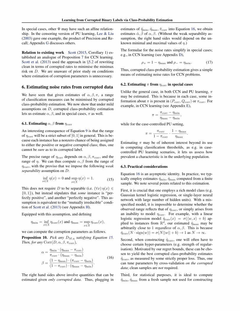
we can compute the corruption parameters as follows.Proposition 10. Pick any DM,η satisfying Equation 15.Then, for any Corr(D,α, β, πcorr),
α =ηmin · (ηmax − πcorr)
πcorr · (ηmax − ηmin)
β =(1− ηmax) · (πcorr − ηmin)
(1− πcorr) · (ηmax − ηmin).
(16)
The right hand sides above involve quantities that can beestimated given only corrupted data. Thus, plugging in
estimates of ηmin, ηmax, πcorr into Equation 16, we obtainestimates α, β of α, β. (Without the weak separability as-sumption, the right hand sides would depend on the un-known minimal and maximal values of η.)
The formulae for the noise rates simplify in special cases;e.g., in CCN learning (see Appendix D),
ρ+ = 1− ηmax and ρ− = ηmin. (17)
Thus, corrupted class-probability estimation gives a simplemeans of estimating noise rates for CCN problems.
6.2. Estimating π from ηcorr in special cases
Unlike the general case, in both CCN and PU learning, πmay be estimated. This is because in each case, some in-formation about π is present in (Pcorr, Qcorr) or πcorr. Forexample, in CCN learning (see Appendix E),
π =πcorr − ηmin
ηmax − ηmin,
while for the case-controlled PU setting,
π =πcorr
1− πcorr· 1− ηmax
ηmax.
Estimating π may be of inherent interest beyond its usein computing classification thresholds, as e.g. in case-controlled PU learning scenarios, it lets us assess howprevalent a characteristic is in the underlying population.
6.3. Practical considerations
Equation 16 is an asymptotic identity. In practice, we typ-ically employ estimates ηmin, ηmax computed from a finitesample. We note several points related to this estimation.
First, it is crucial that one employs a rich model class (e.g.Gaussian kernel logistic regression, or single-layer neuralnetwork with large number of hidden units). With a mis-specified model, it is impossible to determine whether theobserved range reflects that of ηcorr, or simply arises froman inability to model ηcorr. For example, with a linearlogistic regression model ηcorr(x) = σ(〈w, x〉 + b) ap-plied to instances from Rd, our estimated ηmax may bearbitrarily close to 1 regardless of α, β. This is becauseηcorr(N · sign(w)) = σ(N ||w||+ b)→ 1 as N →∞.
Second, when constructing ηcorr, one will often have tochoose certain hyper-parameters (e.g. strength of regular-isation). Motivated by our regret bounds, these can be cho-sen to yield the best corrupted class-probability estimatesηcorr, as measured by some strictly proper loss. Thus, onecan tune parameters by cross-validation on the corrupteddata; clean samples are not required.
Third, for statistical purposes, it is ideal to computeηmin, ηmax from a fresh sample not used for constructing
Learning from Corrupted Binary Labels via Class-Probability Estimation
probability estimates ηcorr. These range estimates mayeven be computed on unlabelled test instances, as they donot require ground truth labels. (This does not constituteoverfitting to the test set, as the underlying model for ηcorr
is learned purely from corrupted training data.)
Fourth, the sample maximum and minimum are clearly sus-ceptible to outliers. Therefore, it may be preferable to em-ploy e.g. the 99% and 1% quantiles as a robust alternative.Alternately, one may perform some form of aggregation(e.g. the bootstrap) to smooth the estimates.
Finally, to compute a suitable threshold for classification,noisy estimates of α, β may be sufficient. For example,in CCN learning, we only need the estimated differenceρ+ − ρ− to be comparable to the true difference ρ+ − ρ−(by Equation 13). du Plessis et al. (2014) performed suchan analysis for the case-controlled PU learning setting.
Relation to existing work The estimator in Equation 16may be seen as a generalisation of that proposed by Elkan& Noto (2008) for the censoring version of PU learning.For CCN learning, in independent work, Liu & Tao (2014,Theorem 4) proposed the estimators in Equation 17.
Scott et al. (2013) proposed a means of estimating the noiseparameters, based on a reduction to the problem of mix-ture proportion estimation. By an interpretation providedby Blanchard et al. (2010), the noise parameters can beseen as arising from the derivative of the right hand side ofthe optimal ROC curve on Corr(D,α, β, πcorr). Sander-son & Scott (2014); Scott (2015) explored a practical es-timator along these lines. As the optimal ROC curve forDcorr is produced by any strictly monotone transformationof ηcorr, class-probability estimation is implicit in this ap-proach, and so our estimator is simply based on a differentperspective. (See Appendix I.) The class-probability esti-mation perspective shows that a single approach can bothestimate the corruption parameters and be used to classifyoptimally for a range of performance measures.
7. ExperimentsWe now present experiments that aim to validate our anal-ysis4 via three questions. First, can we optimise BER andAUC from corrupted data without knowledge of the noiseparameters? Second, can we accurately estimate corrup-tion parameters? Third, can we optimise other classifica-tion measures using estimates of corruption parameters?
We focus on CCN learning with label flip probabilitiesρ+, ρ− ∈ {0, 0.1, 0.2, 0.3, 0.4, 0.49}; recall that ρ− = 0is the censoring version of PU learning. For this prob-
4Sample scripts are available at http://users.cecs.anu.edu.au/˜akmenon/papers/corrupted-labels/index.html.
lem, a number of approaches have been proposed to answerthe third question above, e.g. (Stempfel & Ralaivola, 2007;2009; Natarajan et al., 2013). To our knowledge, all ofthese operate in the setting where the noise parameters areknown. It is thus possible to use the noise estimates fromclass-probability estimation as inputs to these approaches,and we expect such a fusion will be beneficial. We leavesuch a study for future work, as our aim here is merely toillustrate that with corrupted class-probability estimation,we can answer all three questions in the affirmative.
We report results on a range of UCI datasets. For eachdataset, we construct a random 80% – 20% train-test split.For fixed ρ+, ρ−, we inject label noise into the training set.The learner estimates class-probabilities from these noisysamples, with predictions on the clean test samples usedto estimate ηmin, ηmax if required. We summarise perfor-mance across τ independent corruptions of the training set.
Observe that if DM,η can be modelled by a linear scorer,so that η : x 7→ σ(〈w, x〉+ b), then ηcorr : x 7→ (1− ρ+ −ρ−) · σ(〈w, x〉 + b) + ρ−; i.e. , a neural network with asingle hidden sigmoidal unit, bias term, and identity outputlink is well-specified. Thus, in all experiments, we use asour base model a neural network with a sigmoidal hiddenlayer, trained to minimise squared error5 with `2 regular-isation. The regularisation parameter for the model wastuned by cross-validation (on the corrupted data) based onsquared error. We emphasise that both learning and param-eter tuning is solely on corrupted data.
7.1. Are BER and AUC immune to corruption?
We first assess how effectively we can optimise BER andAUC from corrupted data without knowledge or estimatesof the noise parameters. For a fixed setting of ρ+, ρ−,and each of τ = 100 corruption trials, we learn a class-probability estimator from the corrupted training set. Weuse this to predict class-probabilities for instances on theclean test set. We measure the AUC of the resulting class-probabilities, as well as the BER resulting from threshold-ing these probabilities about the corrupted base rate.
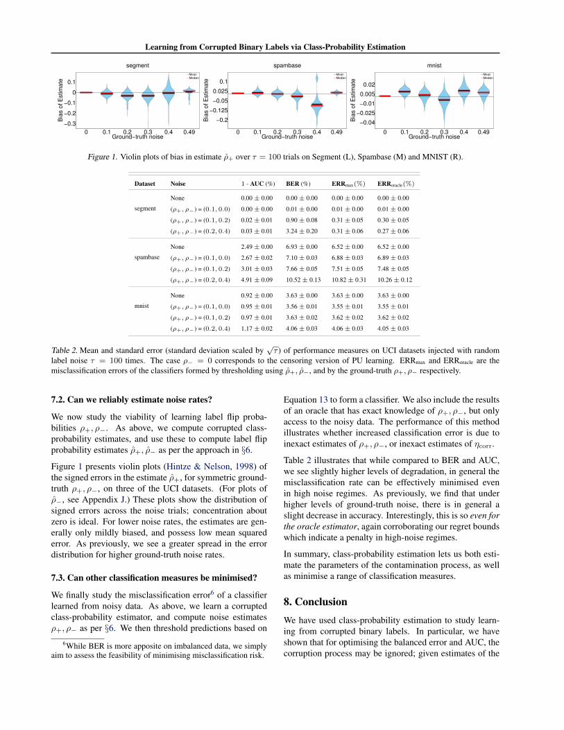
Table 2 summarises the results for a selection of datasetsand noise rates ρ+, ρ−. (Appendix J contains a full set ofresults.) We see that in general the BER and AUC in thenoise-free case (ρ+ = ρ− = 0) and in the noisy casesare commensurate. This is in agreement with our analysison the immunity of BER and AUC. For smaller datasetsand higher levels of noise, we see a greater degradation inperformance. This matches our regret bounds (Proposition2), which indicated a penalty in high-noise regimes.
5Using log-loss requires explicitly constraining the range ofthe bias and hidden→ output term, else the loss is undefined.
Learning from Corrupted Binary Labels via Class-Probability Estimation
0 0.1 0.2 0.3 0.4 0.49
−0.3
−0.2
−0.1
0
0.1
Ground−truth noise
Bia
s o
f E
stim
ate
segment
MeanMedian
0 0.1 0.2 0.3 0.4 0.49
−0.2
−0.125
−0.05
0.025
0.1
Ground−truth noise
Bia
s o
f E
stim
ate
spambase
MeanMedian
0 0.1 0.2 0.3 0.4 0.49
−0.04
−0.025
−0.01
0.005
0.02
Ground−truth noise
Bia
s o
f E
stim
ate
mnist
Mean
Median
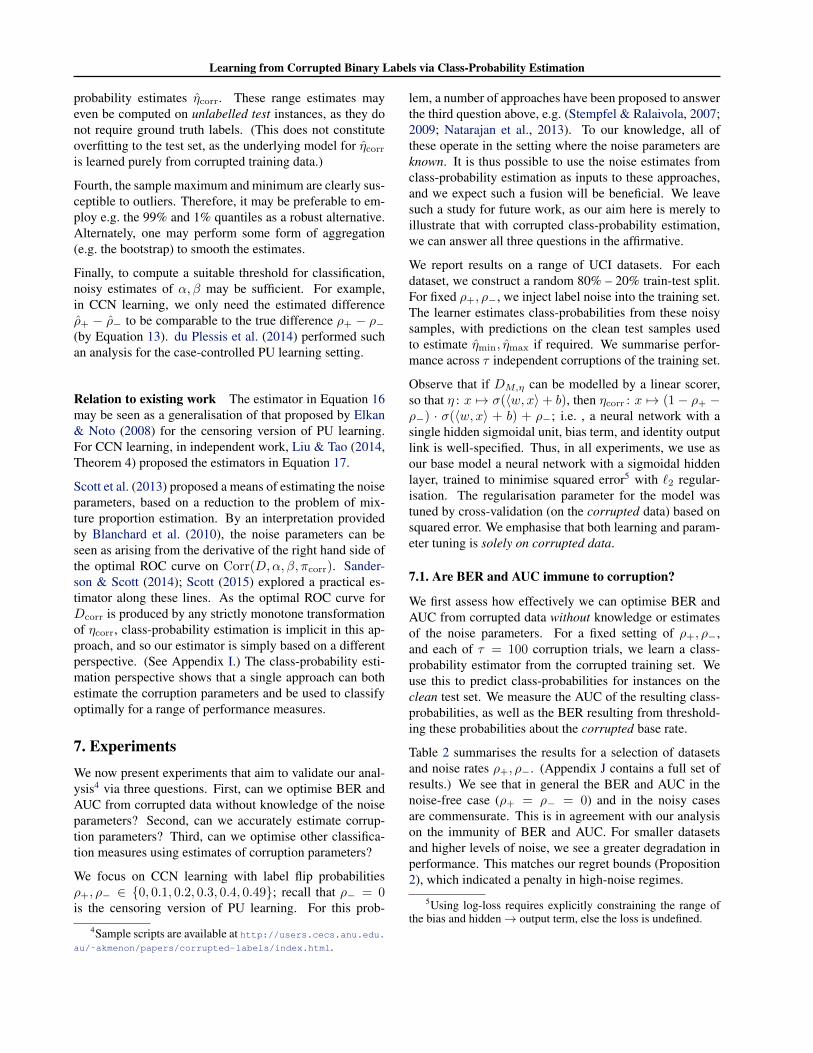
Figure 1. Violin plots of bias in estimate ρ+ over τ = 100 trials on Segment (L), Spambase (M) and MNIST (R).
Dataset Noise 1 - AUC (%) BER (%) ERRmax(%) ERRoracle(%)
segment
None 0.00± 0.00 0.00± 0.00 0.00± 0.00 0.00± 0.00
(ρ+, ρ−) = (0.1, 0.0) 0.00± 0.00 0.01± 0.00 0.01± 0.00 0.01± 0.00
(ρ+, ρ−) = (0.1, 0.2) 0.02± 0.01 0.90± 0.08 0.31± 0.05 0.30± 0.05
(ρ+, ρ−) = (0.2, 0.4) 0.03± 0.01 3.24± 0.20 0.31± 0.06 0.27± 0.06
spambase
None 2.49± 0.00 6.93± 0.00 6.52± 0.00 6.52± 0.00
(ρ+, ρ−) = (0.1, 0.0) 2.67± 0.02 7.10± 0.03 6.88± 0.03 6.89± 0.03
(ρ+, ρ−) = (0.1, 0.2) 3.01± 0.03 7.66± 0.05 7.51± 0.05 7.48± 0.05
(ρ+, ρ−) = (0.2, 0.4) 4.91± 0.09 10.52± 0.13 10.82± 0.31 10.26± 0.12
mnist
None 0.92± 0.00 3.63± 0.00 3.63± 0.00 3.63± 0.00
(ρ+, ρ−) = (0.1, 0.0) 0.95± 0.01 3.56± 0.01 3.55± 0.01 3.55± 0.01
(ρ+, ρ−) = (0.1, 0.2) 0.97± 0.01 3.63± 0.02 3.62± 0.02 3.62± 0.02
(ρ+, ρ−) = (0.2, 0.4) 1.17± 0.02 4.06± 0.03 4.06± 0.03 4.05± 0.03
Table 2. Mean and standard error (standard deviation scaled by√τ ) of performance measures on UCI datasets injected with random
label noise τ = 100 times. The case ρ− = 0 corresponds to the censoring version of PU learning. ERRmax and ERRoracle are themisclassification errors of the classifiers formed by thresholding using ρ+, ρ−, and by the ground-truth ρ+, ρ− respectively.
7.2. Can we reliably estimate noise rates?
We now study the viability of learning label flip proba-bilities ρ+, ρ−. As above, we compute corrupted class-probability estimates, and use these to compute label flipprobability estimates ρ+, ρ− as per the approach in §6.
Figure 1 presents violin plots (Hintze & Nelson, 1998) ofthe signed errors in the estimate ρ+, for symmetric ground-truth ρ+, ρ−, on three of the UCI datasets. (For plots ofρ−, see Appendix J.) These plots show the distribution ofsigned errors across the noise trials; concentration aboutzero is ideal. For lower noise rates, the estimates are gen-erally only mildly biased, and possess low mean squarederror. As previously, we see a greater spread in the errordistribution for higher ground-truth noise rates.
7.3. Can other classification measures be minimised?
We finally study the misclassification error6 of a classifierlearned from noisy data. As above, we learn a corruptedclass-probability estimator, and compute noise estimatesρ+, ρ− as per §6. We then threshold predictions based on
6While BER is more apposite on imbalanced data, we simplyaim to assess the feasibility of minimising misclassification risk.
Equation 13 to form a classifier. We also include the resultsof an oracle that has exact knowledge of ρ+, ρ−, but onlyaccess to the noisy data. The performance of this methodillustrates whether increased classification error is due toinexact estimates of ρ+, ρ−, or inexact estimates of ηcorr.
Table 2 illustrates that while compared to BER and AUC,we see slightly higher levels of degradation, in general themisclassification rate can be effectively minimised evenin high noise regimes. As previously, we find that underhigher levels of ground-truth noise, there is in general aslight decrease in accuracy. Interestingly, this is so even forthe oracle estimator, again corroborating our regret boundswhich indicate a penalty in high-noise regimes.
In summary, class-probability estimation lets us both esti-mate the parameters of the contamination process, as wellas minimise a range of classification measures.
8. ConclusionWe have used class-probability estimation to study learn-ing from corrupted binary labels. In particular, we haveshown that for optimising the balanced error and AUC, thecorruption process may be ignored; given estimates of the
Learning from Corrupted Binary Labels via Class-Probability Estimation
corruption parameters, several classification measures canbe minimised; and that such estimates may be obtained bythe range of the class-probabilities.
In future work, we aim to study the impact of corruption onestimation rates of class-probabilities; study ranking risksbeyond the AUC; and study potential extensions of our re-sults to more general corruption problems.
Acknowledgments. NICTA is funded by the AustralianGovernment through the Department of Communicationsand the Australian Research Council through the ICT Cen-tre of Excellence Program.
ReferencesAgarwal, Shivani. Surrogate regret bounds for bipartite
ranking via strongly proper losses. Journal of MachineLearning Research, 15:1653–1674, 2014.
Agarwal, Shivani, Graepel, Thore, Herbrich, Ralf, Har-Peled, Sariel, and Roth, Dan. Generalization boundsfor the area under the ROC curve. Journal of MachineLearning Research, 6:393–425, December 2005.
Angluin, Dana and Laird, Philip. Learning from noisy ex-amples. Machine Learning, 2(4):343–370, 1988.
Blanchard, Gilles, Lee, Gyemin, and Scott, Clayton. Semi-supervised novelty detection. Journal of Machine Learn-ing Research, 11:2973–3009, December 2010.
Blum, Avrim and Mitchell, Tom. Combining labeled andunlabeled data with co-training. In Conference on Com-putational Learning Theory (COLT), pp. 92–100, NewYork, NY, USA, 1998. ACM. ISBN 1-58113-057-0.
Brodersen, Kay H., Ong, Cheng Soon, Stephan, Klaas E.,and Buhmann, Joachim M. The balanced accuracy andits posterior distribution. In Proceedings of the Inter-national Conference on Pattern Recognition (ICPR), pp.3121–3124, 2010.
Cheng, Jie, Hatzis, Christos, Hayashi, Hisashi, Krogel,Mark-A., Morishita, Shinchi, Page, David, and Sese,Jun. KDD Cup 2001 report. ACM SIGKDD ExplorationsNewsletter, 3(2):47–64, 2002.
Clemencon, Stephan, Lugosi, Gabor, and Vayatis, Nicolas.Ranking and Empirical Minimization of U-statistics. TheAnnals of Statistics, 36(2):844–874, April 2008.
Denis, Francois. PAC learning from positive statisticalqueries. In Algorithmic Learning Theory (ALT), volume1501 of Lecture Notes in Computer Science, pp. 112–126. Springer Berlin Heidelberg, 1998. ISBN 978-3-540-65013-3.
du Plessis, Marthinus C, Niu, Gang, and Sugiyama,Masashi. Analysis of learning from positive and unla-beled data. In Advances in Neural Information Process-ing Systems (NIPS), pp. 703–711. Curran Associates,Inc., 2014.
du Plessis, Marthinus Christoffel and Sugiyama, Masashi.Class prior estimation from positive and unlabeled data.IEICE Transactions, 97-D(5):1358–1362, 2014.
Elkan, Charles and Noto, Keith. Learning classifiers fromonly positive and unlabeled data. In ACM SIGKDDInternational Conference on Knowledge Discovery andData Mining (KDD), pp. 213–220, New York, NY, USA,2008. ACM. ISBN 978-1-60558-193-4.
Flach, Peter, Hernandez-Orallo, Jose, and Ferri, Cesar. Acoherent interpretation of AUC as a measure of aggre-gated classification performance. In International Con-ference on Machine Learning (ICML), 2011.
Guyon, Isabelle, Hur, Asa Ben, Gunn, Steve, and Dror,Gideon. Result analysis of the NIPS 2003 feature selec-tion challenge. In Advances in Neural Information Pro-cessing Systems (NIPS), pp. 545–552. MIT Press, 2004.
Hintze, Jerry L. and Nelson, Ray D. Violin plots: A boxplot-density trace synergism. The American Statistician,52(2):181–184, 1998.
Kotłowski, Wojciech and Dembczynski, Krzysztof. Sur-rogate regret bounds for generalized classification per-formance metrics. In Conference on Learning Theory(COLT), 2015.
Koyejo, Oluwasanmi O, Natarajan, Nagarajan, Raviku-mar, Pradeep K, and Dhillon, Inderjit S. Consistentbinary classification with generalized performance met-rics. In Advances in Neural Information Processing Sys-tems (NIPS), pp. 2744–2752. Curran Associates, Inc.,2014.
Krzanowski, Wojtek J. and Hand, David J. ROC Curves forContinuous Data. Chapman & Hall/CRC, 1st edition,2009. ISBN 1439800219, 9781439800218.
Lee, Wee Sun and Liu, Bing. Learning with Positive andUnlabeled Examples Using Weighted Logistic Regres-sion. In International Conference on Machine Learning(ICML), 2003.
Liu, T. and Tao, D. Classification with Noisy Labels by Im-portance Reweighting. ArXiv e-prints, November 2014.URL http://arxiv.org/abs/1411.7718.
McCullagh, Peter and Nelder, John Ashworth. Generalizedlinear models (Second edition). London: Chapman &Hall, 1989.
Learning from Corrupted Binary Labels via Class-Probability Estimation
Menon, Aditya Krishna, Narasimhan, Harikrishna, Agar-wal, Shivani, and Chawla, Sanjay. On the statisticalconsistency of algorithms for binary classification underclass imbalance. In International Conference on Ma-chine Learning (ICML), pp. 603–611, 2013.
Narasimhan, Harikrishna, Vaish, Rohit, and Agarwal, Shiv-ani. On the statistical consistency of plug-in classi-fiers for non-decomposable performance measures. InAdvances in Neural Information Processing Systems(NIPS), pp. 1493–1501. Curran Associates, Inc., 2014.
Natarajan, Nagarajan, Dhillon, Inderjit S., Ravikumar,Pradeep D., and Tewari, Ambuj. Learning with noisylabels. In Advances in Neural Information ProcessingSystems (NIPS), pp. 1196–1204, 2013.
Parambath, Shameem A. Puthiya, Usunier, Nicolas, andGrandvalet, Yves. Optimizing F-measures by cost-sensitive classification. In Advances in Neural Informa-tion Processing Systems (NIPS), pp. 2123–2131, 2014.
Phillips, Steven J., Dudik, Miroslav, Elith, Jane, Graham,Catherine H., Lehmann, Anthony, Leathwick, John, andFerrier, Simon. Sample selection bias and presence-only distribution models: implications for backgroundand pseudo-absence data. Ecological Applications, 19(1):181–197, 2009.
Reid, Mark D. and Williamson, Robert C. Composite bi-nary losses. Journal of Machine Learning Research, 11:2387–2422, December 2010.
Sanderson, Tyler and Scott, Clayton. Class proportion esti-mation with application to multiclass anomaly rejection.In AISTATS, pp. 850–858, 2014.
Scott, Clayton. A rate of convergence for mixture propor-tion estimation, with application to learning from noisylabels. In To appear in International Conference on Ar-tificial Intelligence and Statistics (AISTATS), 2015.
Scott, Clayton, Blanchard, Gilles, and Handy, Gregory.Classification with asymmetric label noise: Consistencyand maximal denoising. In Conference on Learning The-ory (COLT), volume 30 of JMLR Proceedings, pp. 489–511, 2013.
Stempfel, Guillaume and Ralaivola, Liva. Learning ker-nel perceptrons on noisy data using random projections.In Hutter, Marcus, Servedio, Rocco., and Takimoto,Eiji (eds.), Algorithmic Learning Theory, volume 4754of Lecture Notes in Computer Science, pp. 328–342.Springer Berlin Heidelberg, 2007. ISBN 978-3-540-75224-0.
Stempfel, Guillaume and Ralaivola, Liva. Learning SVMsfrom sloppily labeled data. In Alippi, Cesare, Polycar-pou, Marios, Panayiotou, Christos, and Ellinas, Geor-gios (eds.), Artificial Neural Networks (ICANN), volume5768 of Lecture Notes in Computer Science, pp. 884–893. Springer Berlin Heidelberg, 2009. ISBN 978-3-642-04273-7.
van Rooyen, Brendan and Williamson, Robert C. Learn-ing in the Presence of Corruption. ArXiv e-prints,March 2015. URL http://arxiv.org/abs/1504.00091.
Ward, Gill, Hastie, Trevor, Barry, Simon, Elith, Jane, andLeathwick, John R. Presence-only data and the EM al-gorithm. Biometrics, 65(2):554–563, 2009.
Zhang, Dell and Lee, Wee Sun. Learning classifiers with-out negative examples: A reduction approach. In ThirdInternational Conference on Digital Information Man-agement (ICDIM), pp. 638–643, 2008.
Learning from Corrupted Binary Labels via Class-Probability Estimation
Proofs for “Learning from Corrupted Binary Labels viaClass-Probability Estimation”
A. Additional helper resultsWe collect here some results that are useful for the proofs of results in the main body.
A.1. Basic properties of ηcorr
Corollary 11. Pick any DM,η and Corr(D,α, β, πcorr). Then, ηcorr is a strictly monotone increasing transform of η.
Proof of Corollary 11. Pick any f : R → R, and define the function g : x 7→ a·f(x)+bc·f(x)+d for a, b, c, d ≥ 0. If c = 0, g is
an affine transformation of f , and since a ≥ 0 it is a strictly monotone increasing transformation of f . If c 6= 0, we canrewrite g as
g : x 7→ac · c · f(x) + bc
a ·ac
c · f(x) + d
= x 7→ a
c·c · f(x) + bc
a
c · f(x) + d
= x 7→ a
c·
(1 +
bca − d
c · f(x) + d
)
= x 7→ a
c+
bc− adac · f(x) + ad
.
Since ac ≥ 0, g is a strictly monotone increasing transformation of f when ad > bc.
We now apply this to f(x) = 1−ππ · η(x)
1−η(x) , which is in turn a strictly monotone increasing transformation of η. Then,g = ηcorr, where from Equation 9,
a = (1− α)
b = α
c = β
d = 1− β.
Thus, ad − bc = 1 − α − β, which by our assumption that α + β < 1 is positive. Hence ηcorr is a strictly monotoneincreasing transformation of η.
Corollary 12. Pick any DM,η satisfying Equation 15. Then, for every Corr(D,α, β, πcorr),
ηmin =πcorr · α
1− ρand ηmax =
πcorr · (1− α)
ρ,
where ρ = πcorr · (1− α) + (1− πcorr) · β.
Proof of Corollary 12. For the ρ as defined, it is easy to check that
1− ρ = πcorr · α+ (1− πcorr) · (1− β).
Plug in η(x) = 0 into Equation 9, and we get
ηcorr(x)
1− ηcorr(x)=
πcorr
1− πcorr· α
1− β,
Learning from Corrupted Binary Labels via Class-Probability Estimation
which has solutionηcorr(x) =
πcorr · απcorr · α+ (1− πcorr) · (1− β)
.
Clearly such an x corresponds to the minimum of η, and since ηcorr is a strictly monotone transformation of η by Corollary11, it must correspond to the minimum of ηcorr as well.
Similarly, plug in η(x) = 1 into Equation 9, and we get
ηcorr(x)
1− ηcorr(x)=
πcorr
1− πcorr· 1− α
β,
which has solution
ηcorr(x) =πcorr · (1− α)
πcorr · (1− α) + (1− πcorr) · β.
Proposition 13. Let T : [0, 1]5 → [0, 1] be as per Equation 10. Suppose ∆X×{±1} is the set of all distributions onX× {±1}. The only function t : ∆X×{±1} → [0, 1] for which
(∃F : [0, 1]→ [0, 1]) (∀D,Dcorr)T (α, β, π, πcorr, t(D)) = F (πcorr)
is t : DP,Q,π 7→ π.
Proof of Proposition 13. Let t(D) be some candidate clean threshold function, independent of α, β, πcorr. For conve-nience, let t(D) = t(D)
1−t(D) and g(π) = 1−ππ . Recall from Equation 10 that
(∀D,Dcorr)T (α, β, π, πcorr, t(D))
1− T (α, β, π, πcorr, t(D))=
πcorr
1− πcorr· (1− α) · g(π) · t(D) + α
β · g(π) · t(D) + (1− β).
We require T (α, β, π, πcorr, t(D)) to be equal to F (πcorr) for some function F , or equivalently, to be independent of α, β, π(as well as any other parameters derived from D). Now, as the left hand side of the above equation is a strictly monotonetransformation of T (α, β, π, πcorr, t(D)), we equivalently need the right hand side of the above to be independent ofα, β, π. As the first term, πcorr
1−πcorr, depends solely on πcorr, we need the second term to be independent of α, β, π. Say the
second term equals some function G(πcorr). Then, we require
(∀D,Dcorr) (1− α) · g(π) · t(D) + α = G(πcorr) · (β · g(π) · t(D) + (1− β)).
But then, differentiating this with respect to α, we need
(∀D,Dcorr) − g(π) · t(D) + 1 = 0,
meaning that the only possible solution for t(D) is
t(D) =1
g(π),
or t(D) = π.
Suppose we require T (α, β, π, πcorr, t(D)) to merely be independent of π, but possibly dependent on α, β. For simplicity,suppose t only depends on π. Then, we equivalently need
(∀α, β, π) (1− α) · g(π) · t(π) + α = G(πcorr, α, β) · (β · g(π) · t(π) + (1− β))
for some function G. Differentiating with respect to π, we get that either g(π) · t(π) is a constant (independent of π), orG(πcorr, α, β) = 1−α
β . The latter can be ruled out by plugging back into the original equation, and so we find that theadmissible threshold functions are {
t : π 7→ c0 · π(1− π) + c0 · π
| c0 ∈ R}.
Clearly c0 = 1 corresponds to t(π) = π, but other thresholds (corresponding to non-standard performance measures) arealso possible in this case, e.g. 2π
1+π .
Learning from Corrupted Binary Labels via Class-Probability Estimation
A.2. Contaminated BER and AUC
Corollary 14. Pick any D and Corr(D,α, β, πcorr). Then, for any classifier f : X→ {±1},
Argminf : X→{±1}
BERDcorr(f) = Argminf : X→{±1}
BERD(f)
and
regretDBER(f) =1
1− α− β· regretDcorr
BER (f).
Proof of Corollary 14. As the corrupted BER is a positive scaling and translation of the clean BER (Equation 6), theequivalence of minimisers is immediate.
For the regret relation, observe that
regretDBER(f) = BERD(f)− infg : X→{±1}
BERD(g)
=1
1− α− β·(
BERDcorr(f)− 1
2
)− infg : X→{±1}
1
1− α− β·(
BERDcorr(g)− 1
2
)=
1
1− α− β·(
BERDcorr(f)− infg : X→{±1}
BERDcorr(g)
)=
1
1− α− β· regretDcorr
BER (f).
Corollary 15. For any D and Corr(D,α, β, πcorr),
Argmins : X→R
AUCDcorr(s) = Argmins : X→R
AUCD(s)
and
regretDAUC(s) =1
1− α− β· regretDcorr
AUC (s).
Proof of Corollary 15. Building on Corollary 3, this follows analogously to the proof of Corollary 14.
A.3. Contaminated false positive and negative rates
Proposition 16 ((Scott et al., 2013)). Pick any D and Corr(D,α, β, πcorr). Then, for any classifier f : X→ {±1},
FPRDcorr(f) = (1− β) · FPRD(f)− β · FNRD(f) + β
FNRDcorr(f) = −α · FPRD(f) + (1− α) · FNRD(f) + α,
or equivalently,
FPRD(f) =1
1− α− β·((1− α) · FPRDcorr(f) + β · FNRDcorr(f)− β
)FNRD(f) =
1
1− α− β·(α · FPRDcorr(f) + (1− β) · FNRDcorr(f)− α
).
Proof of Proposition 16. This result essentially appears in Scott et al. (2013), but we find it useful to slightly re-express it
Learning from Corrupted Binary Labels via Class-Probability Estimation
here, and so present a rederivation. Observe that
FPRDcorr(f) = EX∼Qcorr
[Jf(X) = 1K]
= EX∼βP+(1−β)Q
[Jf(X) = 1K]
= β · EX∼P
[Jf(X) = 1K] + (1− β) · EX∼Q
[Jf(X) = 1K]
= β · TPRD(f) + (1− β) · FPRD(f)
= β − β · FNRD(f) + (1− β) · FPRD(f),
and similarly,
FNRDcorr(f) = EX∼Pcorr
[Jf(X) = −1K]
= EX∼(1−α)P+αQ
[Jf(X) = −1K]
= (1− α) · EX∼P
[Jf(X) = −1K] + α · EX∼Q
[Jf(X) = −1K]
= (1− α) · FNRD(f) + α · TNRD(f)
= (1− α) · FNRD(f) + α− α · FPRD(f).
This gives the first part of the result. For the second part, write the above as[FPRDcorr(f)
FNRDcorr(f)
]=
[1− β −β−α 1− α
] [FPRD(f)
FNRD(f)
]+
[βα
].
Inverting this matrix equation gives the second part result.
Lemma 17. Pick any D and Corr(D,α, β, πcorr). Then, for any classifier f : X→ {±1},
ERRD(f) = γ · CSDcorr(f ; c)− π · α+ (1− π) · β1− α− β
,
where
c = φ
(πcorr
1− πcorr· π · α+ (1− π) · (1− α)
π · (1− β) + (1− π) · β
)γ =
1
1− α− β· π · (1− ρ) + ρ · (1− π)
πcorr · (1− πcorr)
ρ = πcorr · (1− α) + (1− πcorr) · β
φ : z 7→ z
1 + z.
Proof of Lemma 17. From Proposition 16,
π · FNRD(f) =π
1− α− β· (α · FPRDcorr(f) + (1− β) · FNRDcorr(f)− α)
(1− π) · FPRD(f) =1− π
1− α− β· ((1− α) · FPRDcorr(f) + β · FNRDcorr(f)− β),
and so
ERRD(f) =π · (1− β) + (1− π) · β
1− α− β· FNRDcorr(f) +
π · α+ (1− π) · (1− α)
1− α− β· FPRDcorr(f) + C,
where C = −π·α+(1−π)·β1−α−β .
Learning from Corrupted Binary Labels via Class-Probability Estimation
But a performance measure of the form
a · FNRDcorr(f) + b · FPRDcorr(f) = πcorr ·a
πcorr· FNRDcorr(f) + (1− πcorr) ·
b
1− πcorr· FPRDcorr(f)
=
(a
πcorr+
b
1− πcorr
)· CSDcorr(f ; c),
where c = b1−πcorr
·(
aπcorr
+ b1−πcorr
)−1
, and
φ−1(c) =c
1− c=
πcorr
1− πcorr· ba.
In our case,
γ =a
πcorr+
b
1− πcorr
=πcorr · (b− a) + a
πcorr · (1− πcorr)
=πcorr · (1− 2π) · (1− α− β) + π · (1− β) + (1− π) · β
πcorr · (1− πcorr)
=(1− π) · ρ+ π · (1− ρ)
πcorr · (1− πcorr)
and
c
1− c=
πcorr
1− πcorr· ba
=πcorr
1− πcorr· π · α+ (1− π) · (1− α)
π · (1− β) + (1− π) · β.
A.4. Strongly proper losses
Proposition 18. Pick any DM,η. Let ` be a strongly proper composite loss with modulus λ. Then, for any s : X→ R,
EX∼M
[(η(X)− ψ−1(s(X)))2
]≤ 2
λ· regretD` (s).
Proof of Proposition 18. An equivalent definition of ` being strongly proper composite with modulus λ is (Agarwal, 2014,Definition 7)
(∀η, η ∈ [0, 1]) regret`(η, η) ≥ λ
2· (η − η)2,
where regret`(η, η) denotes the conditional regret with respect to loss `, so that
regretD` (s) = EX∼M
[regret`(η(X), ψ−1(s(X))
].
Therefore,
EX∼M
[(η(X)− ψ−1(s(X)))2
]≤ 2
λ· regretD` (s).
Learning from Corrupted Binary Labels via Class-Probability Estimation
A.5. Properties of the AUC and BER
We first show the following simple property of the AUC.
Proposition 19. Pick any distribution P over X and scorer s : X→ R. Then,
EX∼P,X′∼P
[Js(X) > s(X′)K +
1
2Js(X) = s(X′)K
]=
1
2.
Proof. Define a distribution D = (P, P, π) over X× {±1} for some π ∈ (0, 1). Then,
AUCD(s) = EX∼P,X′∼P
[Js(X) > s(X′)K +
1
2Js(X) = s(X′)K
].
By the Neyman-Pearson lemma (Clemencon et al., 2008),
Argmins : X→R
1−AUCD(s) = {φ ◦ η | φ strictly monotone increasing }.
But for two identical class-conditionals, η is just a constant, since
(∀x ∈ X)η(x)
1− η(x)=
π
1− π· P (x)
P (x),
or η ≡ π. Therefore,
maxs : X→R
AUCD(s) = AUCD(π) =1
2.
Now consider any other scorer s : X → R. Suppose AUCD(s) < 12 . Then, define the scorer s : x 7→ −s(x). Clearly,
AUCD(s) = 1 − AUCD(s). But if AUCD(s) < 12 , then AUCD(s) > 1
2 . This contradicts the fact that the maximalachievable AUC is 1
2 . Thus, every scorer must attain AUCD(s) = 12 .
Using the above, we show how the AUC can be seen as the average BER for a specific distribution over classificationthresholds. This is implicit in Flach et al. (2011, Theorems 4, 5), but we show the result here for completeness.
Proposition 20. Pick any DP,Q,π. Then,
AUCD(s) =3
2− 2 · E
X∼P
[BERD(s; s(X))
]=
3
2− 2 · E
X∼Q
[BERD(s; s(X))
].
Proof. We use as our starting point the following definition of the AUC (Agarwal et al., 2005):
AUCD(s) = EX∼P,X′∼Q
[Js(X) > s(X′)K +
1
2Js(X) = s(X′)K
].
This can be re-expressed asAUCD(s) = E
X∼P
[1− FPRD(s; s(X))
],
where
FPRD(s; t) = PX′∼Q
(s(X′) > t) +1
2· PX∼Q
(s(X′) = t) ,
which is equivalent to the false positive rate of a randomised classifier that outputs thresh(s, t) when s(x) 6= t, and {±1}uniformly at random when s(x) = t.
Learning from Corrupted Binary Labels via Class-Probability Estimation
Further, by Proposition 19,
EX∼P
[FNRD(s; s(X))
]= E
X∼P,X′∼P
[Js(X) > s(X′)K +
1
2Js(X) = s(X′)K
]=
1
2.
Thus,
EX∼P
[FPRD(s; s(X)) + FNRD(s; s(X))
2
]=
1−AUCD(s) + 12
2,
or
AUCD(s) =3
2− 2 · E
X∼P
[BERD(s; s(X))
].
Equivalently, we haveAUCD(s) = E
X∼Q
[1− FNRD(s; s(X))
]and by Proposition 19,
EX∼Q
[FPRD(s; s(X))
]= E
X∼Q,X′∼Q
[Js(X′) > s(X)K +
1
2Js(X′) = s(X)K
]=
1
2.
Thus,
EX∼Q
[FPRD(s; s(X)) + FNRD(s; s(X))
2
]=
1−AUCD(s) + 12
2,
or
AUCD(s) =3
2− 2 · E
X∼Q
[BERD(s; s(X))
].
Observe that the above implies a special property of the BER.
Corollary 21. Pick any DP,Q,π and scorer s : X→ R. Then,
EX∼P
[BERD(s; s(X))
]= E
X∼Q
[BERD(s; s(X))
].
B. Proofs of results in main bodyWe now present proofs of all results in the main body.
B.1. BER and AUC are immune to corruption
Proof of Proposition 1. Recalling from Proposition 16 that for any classifier f : X→ {±1},
FPRD(f) =1
1− α− β·((1− α) · FPRDcorr(f) + β · FNRDcorr(f)− β
)FNRD(f) =
1
1− α− β·(α · FPRDcorr(f) + (1− β) · FNRDcorr(f)− α
),
the result follows immediately by definition of the BER as the mean of the false positive and negative rates.
Learning from Corrupted Binary Labels via Class-Probability Estimation
Proof of Proposition 2. Define ηcorr : x 7→ ψ−1(s(x)). For some fixed c ∈ (0, 1), let f = thresh(s, ψ(c)) =thresh(ηcorr, c). By Menon et al. (2013, Lemma 4),
regretDcorr
CS(c)(f) ≤ minr≥1
(E
X∼Mcorr
[|ηcorr(X)− ηcorr(X)|r])1/r
,
where regretDcorr
CS(c)(f) denotes the regret with respect to the cost-sensitive loss with parameter c,
CS(f ; c) = π · (1− c) · FNRD(f) + (1− π) · c · FPRD(f).
The BER of f with respect to distribution Dcorr can be viewed as a scaled version cost-sensitive loss with cost parameterc = πcorr:
BERDcorr(f) =1
2 · πcorr · (1− πcorr)· CS(f ;πcorr).
So, by Corollary 14,
regretDBER(f) =1
1− α− β· regretDcorr
BER (f)
=1
1− α− β· 1
2 · πcorr · (1− πcorr)· regretDcorr
CS(c)(f)
≤ 1
1− α− β· 1
2 · πcorr · (1− πcorr)·minr≥1
(E
X∼Mcorr
[|ηcorr(X)− ηcorr(X)|r])1/r
.
If ` is strongly proper composite with modulus λ, then by Proposition 18,
√E
X∼Mcorr
[(ηcorr(X)− ηcorr(X))2] ≤√
2
λ·√
regretDcorr
` (s).
But the left hand side corresponds to the case of r = 2 in the above bound, meaning
regretDBER(f) ≤ C(πcorr)
1− α− β·√
2
λ·√
regretDcorr
` (s).
Proof of Corollary 3. Using the results of Appendix A.5, we have
AUCDcorr(s) =3
2− 2 · E
X∼Pcorr
[BERDcorr(s; s(X))
]=
3
2− 2 · E
X∼Pcorr
[1
2+ (1− α− β) ·
(BERD(s; s(X))− 1
2
)]=
3
2− (α+ β)− 2 · (1− α− β) · E
X∼Pcorr
[BERD(s; s(X))
]=
1
2+ (1− α− β)− 2 · (1− α− β) ·
((1− α) · E
X∼P
[BERD(s; s(X))
]+ α · E
X∼Q
[BERD(s; s(X))
])=
1
2+ (1− α− β)− 2 · (1− α− β) · E
X∼P
[BERD(s; s(X))
]=
1
2+ (1− α− β) + (1− α− β) ·AUCD(s)− 3
2· (1− α− β)
=1
2+ (1− α− β) ·
(AUCD(s)− 1
2
).
Learning from Corrupted Binary Labels via Class-Probability Estimation
Proof of Corollary 4. From Corollary 15, we know that
regretDAUC(s) =1
1− α− β· regretDcorr
AUC (s).
Now apply Agarwal (2014, Theorem 13) to the right hand side.
B.2. The corrupted class-probabilities
Proof of Proposition 5. Let p, q denotes the densities of P,Q, and pcorr, qcorr the densities of Pcorr, Qcorr. By the definitionof conditional probability, we have
p(x)
q(x)=
1− ππ· η(x)
1− η(x).
and, on the corrupted distribution,ηcorr(x)
1− ηcorr(x)=
πcorr
1− πcorr· pcorr(x)
qcorr(x).
Thus, from Equation 2,
(∀x ∈ X)ηcorr(x)
1− ηcorr(x)=
πcorr
1− πcorr· (1− α) · p(x) + α · q(x)
β · p(x) + (1− β) · q(x)
=πcorr
1− πcorr·
(1− α) · p(x)q(x) + α
β · p(x)q(x) + (1− β)
=πcorr
1− πcorr·
(1− α) · 1−ππ ·
η(x)1−η(x) + α
β · 1−ππ ·
η(x)1−η(x) + (1− β)
.
Proof of Corollary 6. This follows from the fact that ηcorr is a strictly monotone increasing transformation of η (Corollary11), and plugging in η(x) = t into Equation 9.
B.3. Classification from corrupted data
Proof of Proposition 7. Define ηcorr : x 7→ ψ−1(s(x)), and let f = thresh(ηcorr, tDcorr,Ψ). Now, recall from Lemma 17
that
ERRD(f) = γ · CSDcorr(f ; c)− π · α+ (1− π) · β1− α− β
where the cost parameter c = tDcorr,Ψ. Thus,
regretDERR(f) = γ · regretDcorr
CS(c)(f).
The rest of the proof proceeds identically to that of Proposition 2.
Proof of Proposition 8. ( ⇐= ). For Ψ corresponding to the BER, we know from Proposition 1 that this holds for theidentity function F : πcorr 7→ πcorr.
( =⇒ ). Suppose Ψ satisfies the desired statement. Since Ψ has a unique minimiser which is a thresholding of ηcorr, andsince η and ηcorr are strict monotone transformations of each other, we can conclude that for every D, Ψ has a uniqueminimiser of the form sign(η(x)− tDΨ) for some tDΨ . By Corollary 6, we have that
(∀D,Dcorr) (∀x ∈ X) sign(η(x)− tDΨ) = sign(ηcorr(x)− T (α, β, π, πcorr, tDΨ)).
Thus, by assumption on the minimiser of Ψ,
(∃F ) (∀D,Dcorr) (∀x ∈ X) sign(ηcorr(x)− T (α, β, π, πcorr, tDΨ)) = sign(ηcorr(x)− F (πcorr)).
Learning from Corrupted Binary Labels via Class-Probability Estimation
Thus, it must be true that(∃F ) (∀D,Dcorr)F (πcorr) = T (α, β, π, πcorr, t
DΨ).
Now, by Proposition 13, we must have that tDΨ = π. But this corresponds to the unique optimal threshold for the BER.Hence, Ψ must correspond to the BER.
Proof of Proposition 9. Given some w : [0, 1]→ R2+, we restrict attention to functions of the form7
Ψw : (u, v, p) 7→⟨w(p),
[uv
]⟩,
with corresponding performance measures of the form
ClassDΨw(f) = w1(π) · FPRD(f) + w2(π) · FNRD(f).
We are interested in admissible weights w, for which the performance measures on the clean and corrupted distributionsare some affine transformation on each other:
W = {w : [0, 1]→ R2+ | (∀D) (∀α, β, πcorr)(∃a, b ∈ R) (∀f) ClassDΨw
(f) = a · ClassDcorr
Ψw(f) + b}
= {w : [0, 1]→ R2+ | (∀D) (∀α, β, πcorr)(∃a, b ∈ R) (∀f) 〈w(π), x〉 = a · 〈w(πcorr), x〉+ b},
where we let x =
[FPRD(f)
FNRD(f)
], and x =
[FPRDcorr(f)
FNRDcorr(f)
]. Observe that a, b are allowed to depend on the distribution
D, and the corruption process parameters. What is relevant is that they do not depend on the classifier f , so that for thepurposes of minimising Ψ on D, we can equivalently minimise Ψ on Dcorr.
Recall from Proposition 16 that, for any D,Dcorr, f ,[FPRDcorr(f)
FNRDcorr(f)
]=
[1− β −β−α 1− α
] [FPRD(f)
FNRD(f)
]+
[βα
],
or, in the preceding notation,x = Ax+ c
where
A =
[1− β −β−α 1− α
]c =
[βα
].
Pick any w ∈ R2+
[0,1]. Then, we have
w ∈W ⇐⇒ (∀DP,Q,π) (∀α, β, πcorr) (∃a, b) (∀f) 〈w(π), x〉 = a · 〈w(πcorr), Ax+ c〉+ b.
As this must hold for every choice of πcorr, it must hold for the case πcorr = π, i.e.
w ∈W =⇒ (∀DP,Q,π) (∀α, β) (∃a, b) (∀f) 〈w(π), x〉 = a · 〈w(π), Ax+ c〉+ b.
For any π ∈ (0, 1), we can pick (P,Q) such that D is separable. For a separable D, we can pick a classifier so as to attainany combination of false-positive and negative rates (possibly by allowing for randomised classifiers). For x =
[0 0
],
we see that b = −a · 〈w(π), c〉. So,
w ∈W =⇒ (∀π) (∀α, β) (∃a) (∀x ∈ [0, 1]2) 〈w(π), x〉 = a · 〈ATw(π), x〉
=⇒ (∀π) (∀α, β) (∃a) (∀x ∈ [0, 1]2)
⟨(1
aI −AT
)w(π), x
⟩= 0.
7We assume here for simplicity that the performance measure is such that Ψ(0, 0, p) = 0; adding any constant to Ψ will triviallyleave the following unchanged.
Learning from Corrupted Binary Labels via Class-Probability Estimation
As this must hold for every x ∈ [0, 1]2, this is satisfiable iff the first term is zero, i.e.
w ∈W =⇒ (∀π) (∀α, β) (∃a)ATw(π) =1
aIw(π).
This is possible only if w(π) is some scaling of an eigenvector of AT , or is in the nullspace of AT . But
AT =
[1− β −α−β 1− α
],
which is a scaled row-stochastic matrix. Since α + β 6= 1, it is invertible and hence has empty nullspace. Its eigenvectors
are[11
]and
[1
−β/α
]. The latter depends on α, β, which is not possible since w does not depend on these parameters. So,
W ⊆{w : π 7→
[λ(π)λ(π)
]| λ : [0, 1]→ R
}.
The above is in fact an equality. Pick any w : π 7→[λ(π) λ(π)
]T. Then, for any D,Dcorr, and classifier f ,
〈w(πcorr), Ax+ c〉 = λ(πcorr) ·⟨[
11
], Ax+ c
⟩= λ(πcorr) ·
⟨AT[11
], x
⟩+ λ(πcorr) ·
⟨[11
], c
⟩= λ(πcorr) · (1− α− β) ·
⟨[11
], x
⟩+ λ(πcorr) ·
⟨[11
], c
⟩=λ(πcorr)
λ(π)· (1− α− β) ·
⟨λ(π) ·
[11
], x
⟩+ λ(πcorr) ·
⟨[11
], c
⟩= a · 〈w(π), x〉+ b
for appropriate a, b, so that w ∈W. Thus,
W =
{w : π 7→
[λ(π)λ(π)
]| λ : [0, 1]→ R
}.
These correspond to the performance measures
ClassDw (f) = λ(π) · (FPRD(f) + FNRD(f)) = 2λ(π) · BERD(f),
meaning that the set of admissible functionals is the set of scalings and translations of balanced error.
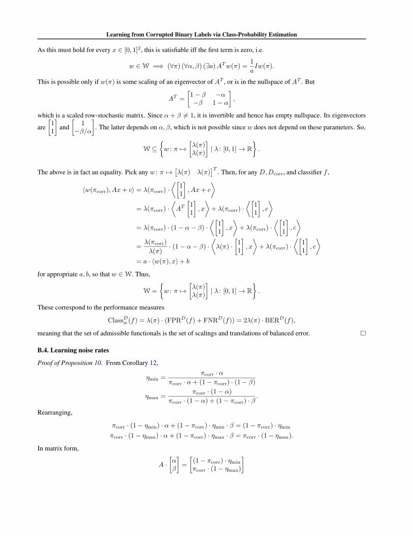
B.4. Learning noise rates
Proof of Proposition 10. From Corollary 12,
ηmin =πcorr · α
πcorr · α+ (1− πcorr) · (1− β)
ηmax =πcorr · (1− α)
πcorr · (1− α) + (1− πcorr) · β.
Rearranging,
πcorr · (1− ηmin) · α+ (1− πcorr) · ηmin · β = (1− πcorr) · ηmin
πcorr · (1− ηmax) · α+ (1− πcorr) · ηmax · β = πcorr · (1− ηmax).
In matrix form,
A ·[αβ
]=
[(1− πcorr) · ηmin
πcorr · (1− ηmax)
]
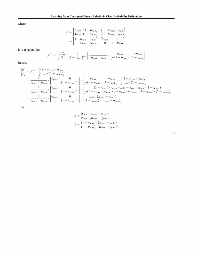
Learning from Corrupted Binary Labels via Class-Probability Estimation
where
A =
[πcorr · (1− ηmin) (1− πcorr) · ηmin
πcorr · (1− ηmax) (1− πcorr) · ηmax
]=
[1− ηmin ηmin
1− ηmax ηmax
]·[πcorr 0
0 1− πcorr
].
It is apparent that
A−1 =
[π−1
corr 00 (1− πcorr)
−1
]· 1
ηmax − ηmin·[
ηmax −ηmin
−(1− ηmax) 1− ηmin
]Hence,[
αβ
]= A−1 ·
[(1− πcorr) · ηmin
πcorr · (1− ηmax)
]=
1
ηmax − ηmin·[π−1
corr 00 (1− πcorr)
−1
]·[
ηmax −ηmin
−(1− ηmax) 1− ηmin
]·[
(1− πcorr) · ηmin
πcorr · (1− ηmax)
]=
1
ηmax − ηmin·[π−1
corr 00 (1− πcorr)
−1
]·[
(1− πcorr) · ηmax · ηmin − πcorr · ηmin · (1− ηmax)−(1− πcorr) · ηmin · (1− ηmax) + πcorr · (1− ηmin) · (1− ηmax)
]=
1
ηmax − ηmin·[π−1
corr 00 (1− πcorr)
−1
]·[
ηmin · (ηmax − πcorr)(1− ηmax) · (πcorr − ηmin)
].
Thus,
α =ηmin · (ηmax − πcorr)
πcorr · (ηmax − ηmin)
β =(1− ηmax) · (πcorr − ηmin)
(1− πcorr) · (ηmax − ηmin).
Learning from Corrupted Binary Labels via Class-Probability Estimation
Additional Discussion for “Learning from Corrupted BinaryLabels via Class-Probability Estimation”
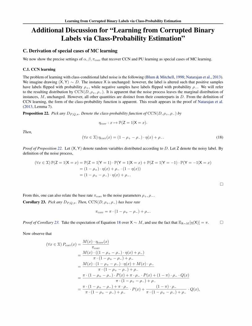
C. Derivation of special cases of MC learningWe now show the precise settings of α, β, πcorr that recover CCN and PU learning as special cases of MC learning.
C.1. CCN learning
The problem of learning with class-conditional label noise is the following (Blum & Mitchell, 1998; Natarajan et al., 2013).We imagine drawing (X,Y) ∼ D. The instance X is unchanged: however, the label is altered such that positive sampleshave labels flipped with probability ρ+, while negative samples have labels flipped with probability ρ−. We will referto the resulting distribution by CCN(D, ρ+, ρ−). It is apparent that the noise process leaves the marginal distribution ofinstances, M , unchanged. However, all other quantities are distinct from their counterparts in D. From the definition ofCCN learning, the form of the class-probability function is apparent. This result appears in the proof of Natarajan et al.(2013, Lemma 7).
Proposition 22. Pick any DP,Q,π. Denote the class-probability function of CCN(D, ρ+, ρ−) by
ηcorr : x 7→ P(Z = 1|X = x).
Then,(∀x ∈ X) ηcorr(x) = (1− ρ+ − ρ−) · η(x) + ρ−. (18)
Proof of Proposition 22. Let (X,Y) denote random variables distributed according to D. Let Z denote the noisy label. Bydefinition of the noise process,
(∀x ∈ X)P(Z = 1|X = x) = P(Z = 1|Y = 1) · P(Y = 1|X = x) + P(Z = 1|Y = −1) · P(Y = −1|X = x)
= (1− ρ+) · η(x) + ρ− · (1− η(x))
= (1− ρ+ − ρ−) · η(x) + ρ−.
From this, one can also relate the base rate πcorr to the noise parameters ρ+, ρ−.
Corollary 23. Pick any DP,Q,π . Then, CCN(D, ρ+, ρ−) has base rate
πcorr = π · (1− ρ+ − ρ−) + ρ−.
Proof of Corollary 23. Take the expectation of Equation 18 over X ∼M , and use the fact that EX∼M [η(X)] = π.
Now observe that
(∀x ∈ X)Pcorr(x) =M(x) · ηcorr(x)
πcorr
=M(x) · ((1− ρ+ − ρ−) · η(x) + ρ−)
π · (1− ρ+ − ρ−) + ρ−
=M(x) · (1− ρ+ − ρ−) · η(x) +M(x) · ρ−
π · (1− ρ+ − ρ−) + ρ−
=π · (1− ρ+ − ρ−) · P (x) + π · ρ− · P (x) + (1− π) · ρ− ·Q(x)
π · (1− ρ+ − ρ−) + ρ−
=π · (1− ρ+ − ρ−) + π · ρ−π · (1− ρ+ − ρ−) + ρ−
· P (x) +(1− π) · ρ−
π · (1− ρ+ − ρ−) + ρ−·Q(x),
Learning from Corrupted Binary Labels via Class-Probability Estimation
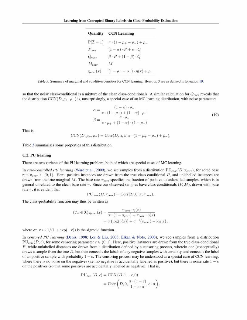
Quantity CCN Learning
P(Z = 1) π · (1− ρ+ − ρ−) + ρ−
Pcorr (1− α) · P + α ·Q
Qcorr β · P + (1− β) ·Q
Mcorr M
ηcorr(x) (1− ρ+ − ρ−) · η(x) + ρ−
Table 3. Summary of marginal and condition densities for CCN learning. Here, α, β are as defined in Equation 19.
so that the noisy class-conditional is a mixture of the clean class-conditionals. A similar calculation for Qcorr reveals thatthe distribution CCN(D, ρ+, ρ−) is, unsurprisingly, a special case of an MC learning distribution, with noise parameters
α =(1− π) · ρ−
π · (1− ρ+) + (1− π) · ρ−β =
π · ρ+
π · ρ+ + (1− π) · (1− ρ−).
(19)
That is,CCN(D, ρ+, ρ−) = Corr(D,α, β, π · (1− ρ+ − ρ−) + ρ−).
Table 3 summarises some properties of this distribution.
C.2. PU learning
There are two variants of the PU learning problem, both of which are special cases of MC learning.
In case-controlled PU learning (Ward et al., 2009), we see samples from a distribution PUcase(D,πcorr), for some baserate πcorr ∈ (0, 1). Here, positive instances are drawn from the true class-conditional P , and unlabelled instances aredrawn from the true marginal M . The base rate πcorr specifies the fraction of positive to unlabelled samples, which is ingeneral unrelated to the clean base rate π. Since our observed samples have class-conditionals (P,M), drawn with baserate π, it is evident that
PUcase(D,πcorr) = Corr(D, 0, π, πcorr).
The class-probability function may thus be written as
(∀x ∈ X) ηcorr(x) =πcorr · η(x)
π · (1− πcorr) + πcorr · η(x)
= σ(log(η(x)) + σ−1(πcorr)− log π
),
where σ : x 7→ 1/(1 + exp(−x)) is the sigmoid function.
In censored PU learning (Denis, 1998; Lee & Liu, 2003; Elkan & Noto, 2008), we see samples from a distributionPUcen (D, c), for some censoring parameter c ∈ (0, 1). Here, positive instances are drawn from the true class-conditionalP , while unlabelled distances are drawn from a distribution defined by a censoring process, wherein one (conceptually)draws a sample from the true D, but then conceals the labels of any negative samples with certainty, and conceals the labelof an positive sample with probability 1− c. The censoring process may be understood as a special case of CCN learning,where there is no noise on the negatives (i.e. no negative is accidentally labelled as positive), but there is noise rate 1 − con the positives (so that some positives are accidentally labelled as negative). That is,
PUcen (D, c) = CCN (D, 1− c, 0)
= Corr
(D, 0,
π · (1− c)1− c · π
, c · π).
Learning from Corrupted Binary Labels via Class-Probability Estimation
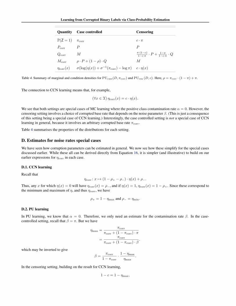
Quantity Case controlled Censoring
P(Z = 1) πcorr c · π
Pcorr P P
Qcorr M π·(1−c)1−c·π · P + 1−π
1−c·π ·Q
Mcorr ρ · P + (1− ρ) ·Q M
ηcorr(x) σ(log(η(x)) + σ−1(πcorr)− log π) c · η(x)
Table 4. Summary of marginal and condition densities for PUcase(D,πcorr) and PUcen (D, c). Here, ρ = πcorr · (1− π) + π.
The connection to CCN learning means that, for example,
(∀x ∈ X) ηcorr(x) = c · η(x).
We see that both settings are special cases of MC learning where the positive class contamination rate α = 0. However, thecensoring setting involves a choice of corrupted base rate that depends on the noise parameter β. (This is just a consequenceof this setting being a special case of CCN learning.) Interestingly, the case controlled setting is not a special case of CCNlearning in general, because it involves an arbitrary corrupted base rate πcorr.
Table 4 summarises the properties of the distributions for each setting.
D. Estimates for noise rates special casesWe have seen how corruption parameters can be estimated in general. We now see how these simplify for the special casesdiscussed earlier. While these all can be derived directly from Equation 16, it is simpler (and illustrative) to build on ourearlier expressions for ηcorr in each case.
D.1. CCN learning
Recall thatηcorr : x 7→ (1− ρ+ − ρ−) · η(x) + ρ−.
Thus, any x for which η(x) = 0 will have ηcorr(x) = ρ−, and if η(x) = 1, ηcorr(x) = 1− ρ+. Since these correspond tothe minimum and maximum of η, and thus ηcorr, we have
ρ+ = 1− ηmax and ρ− = ηmin.
D.2. PU learning
In PU learning, we know that α = 0. Therefore, we only need an estimate for the contamination rate β. In the case-controlled setting, recall that β = π. But we have
ηmax =πcorr
πcorr + (1− πcorr) · π
=πcorr
πcorr + (1− πcorr) · β.
which may be inverted to give
β =πcorr
1− πcorr· 1− ηmax
ηmax.
In the censoring setting, building on the result for CCN learning,
1− c = 1− ηmax,
Learning from Corrupted Binary Labels via Class-Probability Estimation
orc = ηmax.
This is precisely one of the estimators proposed by Elkan & Noto (2008).
E. Estimates for π in special casesWe show how π can be estimated in each of the special cases discussed earlier.
E.1. CCN learning
In the CCN learning scenario, we have
π =πcorr − ρ−
1− ρ+ − ρ−.
That is, the base rate contains information about π, unlike the general MC learning problem. Using the estimates for ρ+, ρ−from earlier, we can thus estimate π from ηcorr as
π =πcorr − ηmin
ηmax − ηmin.
E.2. PU learning
In the case-controlled scenario, we have α = 0 and β = π. Therefore, estimating β is equivalent to estimating π. Recallingour earlier estimate for β, we have
π =πcorr
1− πcorr· 1− ηmax
ηmax.
This does not contradict Ward et al. (2009, Proposition 7), which states that π is unidentifiable when using linear logisticregression to model an arbitrary η (i.e. when using a misspecified model). This reiterates the importance of our assumptionof a suitably rich function class, as well as the weak separability assumption D.
In the censoring scenario, using the result for CCN learning, we have the following, which is mentioned in Elkan & Noto(2008, Section 3):
π =πcorr
ηmax.
F. Thresholds for misclassification error in special casesThe optimal corrupted threshold for the misclassification error simplifies in the special cases discussed earlier.
F.1. CCN learning
From the definition of ηcorr, it is apparent that
(∀x ∈ X) η(x) > t ⇐⇒ ηcorr(x) > (1− ρ+ − ρ−) · t+ ρ−.
Setting t = 12 ,
(∀x ∈ X) η(x) >1
2⇐⇒ ηcorr(x) >
1− ρ+ + ρ−2
.
It is apparent that the only choice of noise rates for which the contaminated threshold is a constant is ρ+ = ρ−, i.e. thesymmetric noise case.
F.2. PU learning
In the case-controlled setting, from the definition of ηcorr, it is apparent that
(∀x ∈ X) η(x) > t ⇐⇒ ηcorr(x) >πcorr · t
πcorr · t+ (1− πcorr) · π.
Learning from Corrupted Binary Labels via Class-Probability Estimation
Setting t = 12 ,
(∀x ∈ X) η(x) >1
2⇐⇒ ηcorr(x) >
πcorr
πcorr + 2 · (1− πcorr) · π.
Recall that π can be expressed in terms of πcorr and ηmax. Plugging this in, we find
(∀x ∈ X) η(x) >1
2⇐⇒ ηcorr(x) >
ηmax
2− ηmax.
In general this is not a constant, and we cannot avoid the estimation of ηmax.
In the censoring setting, plugging in ρ+ = 1− c and ρ− = 0 into the CCN formula,
(∀x ∈ X) η(x) >1
2⇐⇒ ηcorr(x) >
c
2.
It is apparent that we thus always need to estimate the censoring rate in order to optimally threshold. This also followsfrom the fact that the problem is a form of asymmetric label noise, which we saw above yields a non-constant corruptedthreshold.
G. Noise immunity in special casesWe study whether in special cases, there are performance measures other than BER that are immune to corruption.
G.1. CCN learning
For CCN learning with arbitrary label noise, as before, we consider a clean threshold function t(π) on η such that thecorresponding contaminated threshold T (α, β, π, πcorr, t(π)) depends only on πcorr (i.e. is independent of ρ+, ρ−, π). Asin the general case, the only such threshold is t(π) = π.
Proposition 24. For CCN learning with arbitrary label noise, the only function t(π) for which T (α, β, π, πcorr, t(π)) isindependent of ρ+, ρ−, π is t(π) = π, i.e. the optimal threshold for BER.
Proof. From the definition of ηcorr, it is apparent that
T (α, β, π, πcorr, t) = (1− ρ+ − ρ−) · t+ ρ−.
For noise-immunity, we want the corrupted threshold to be some function of πcorr (and thus independent of ρ+, ρ−, π)when given a clean threshold t(π). Recall that πcorr = (1− ρ+− ρ−) · π+ ρ− is itself a function of ρ+, ρ−, π. So, we areinterested in all choices of clean threshold t(π) such that
(∀ρ+, ρ−, π) (1− ρ+ − ρ−) · t(π) + ρ− = F ((1− ρ+ − ρ−) · π + ρ−)
for some function F .
Plug in π = 0 in the above and we get(∀ρ+, ρ−) ρ− = F (ρ−).
That is, the only feasible choice of F is the identity function. Thus,
(∀ρ+, ρ−, π) (1− ρ+ − ρ−) · t(π) + ρ− = (1− ρ+ − ρ−) · π + ρ−,
or(∀ρ+, ρ−, π) (1− ρ+ − ρ−) · (t(π)− π) = 0.
Fix any ρ+, ρ− such that ρ+ + ρ− 6= 1, and we need
(∀π) t(π)− π = 0.
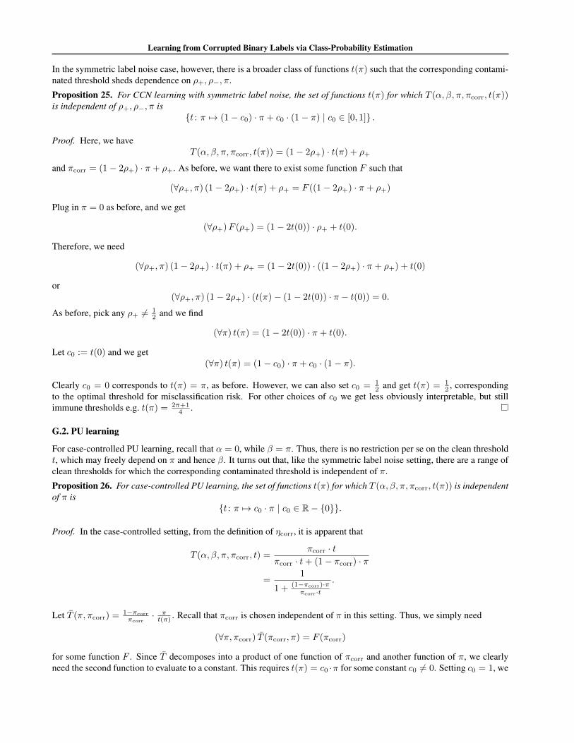
Learning from Corrupted Binary Labels via Class-Probability Estimation
In the symmetric label noise case, however, there is a broader class of functions t(π) such that the corresponding contami-nated threshold sheds dependence on ρ+, ρ−, π.
Proposition 25. For CCN learning with symmetric label noise, the set of functions t(π) for which T (α, β, π, πcorr, t(π))is independent of ρ+, ρ−, π is
{t : π 7→ (1− c0) · π + c0 · (1− π) | c0 ∈ [0, 1]} .
Proof. Here, we haveT (α, β, π, πcorr, t(π)) = (1− 2ρ+) · t(π) + ρ+
and πcorr = (1− 2ρ+) · π + ρ+. As before, we want there to exist some function F such that
(∀ρ+, π) (1− 2ρ+) · t(π) + ρ+ = F ((1− 2ρ+) · π + ρ+)
Plug in π = 0 as before, and we get
(∀ρ+)F (ρ+) = (1− 2t(0)) · ρ+ + t(0).
Therefore, we need
(∀ρ+, π) (1− 2ρ+) · t(π) + ρ+ = (1− 2t(0)) · ((1− 2ρ+) · π + ρ+) + t(0)
or(∀ρ+, π) (1− 2ρ+) · (t(π)− (1− 2t(0)) · π − t(0)) = 0.
As before, pick any ρ+ 6= 12 and we find
(∀π) t(π) = (1− 2t(0)) · π + t(0).
Let c0 := t(0) and we get(∀π) t(π) = (1− c0) · π + c0 · (1− π).
Clearly c0 = 0 corresponds to t(π) = π, as before. However, we can also set c0 = 12 and get t(π) = 1
2 , correspondingto the optimal threshold for misclassification risk. For other choices of c0 we get less obviously interpretable, but stillimmune thresholds e.g. t(π) = 2π+1
4 .
G.2. PU learning
For case-controlled PU learning, recall that α = 0, while β = π. Thus, there is no restriction per se on the clean thresholdt, which may freely depend on π and hence β. It turns out that, like the symmetric label noise setting, there are a range ofclean thresholds for which the corresponding contaminated threshold is independent of π.
Proposition 26. For case-controlled PU learning, the set of functions t(π) for which T (α, β, π, πcorr, t(π)) is independentof π is
{t : π 7→ c0 · π | c0 ∈ R− {0}}.
Proof. In the case-controlled setting, from the definition of ηcorr, it is apparent that
T (α, β, π, πcorr, t) =πcorr · t
πcorr · t+ (1− πcorr) · π
=1
1 + (1−πcorr)·ππcorr·t
.
Let T (π, πcorr) = 1−πcorr
πcorr· πt(π) . Recall that πcorr is chosen independent of π in this setting. Thus, we simply need
(∀π, πcorr) T (πcorr, π) = F (πcorr)
for some function F . Since T decomposes into a product of one function of πcorr and another function of π, we clearlyneed the second function to evaluate to a constant. This requires t(π) = c0 ·π for some constant c0 6= 0. Setting c0 = 1, we
Learning from Corrupted Binary Labels via Class-Probability Estimation
get the BER-optimal threshold t(π) = π. For other choices of the constant, we get thresholds corresponding to functionalsof the form
π · (1− c0 · π) · FPRD(f) + (1− π) · c0 · π · FNRD(f).
Recall that the censoring setting is a special case of CCN learning with asymmetric label noise. Thus, from the previousresults, we see that the only clean threshold that does not require estimating the censoring parameter is t(π) = π. As notedin the body, a qualification is in order, which we now discuss.
G.3. When do performance measure equivalences hold in the censoring setting?
We show that for the purposes of minimising a performance measure on the clean distribution, it is possible to have acorrupted threshold that depends on the corruption parameters, but that we can nonetheless estimate this threshold withouthaving to estimate the corruption parameters. We do this by operating in the censoring version of PU learning, whichsimplifies a lot of the analysis. Consider
Ψ: (u, v, p) 7→ (1− y)2
p · (1− y) + (1− p) · x, (20)
so that
ClassDΨ(f) =(TPRD(f))2
π · TPRD(f) + (1− π) · FPRD(f).
The denominator is subtly different from the misclassification risk, and in fact is simply PX∼M (f(X) = 1). Lee & Liu(2003) showed that, in the censoring setting,
ClassDΨ(f) = ClassPUcen(D,c)Ψ (f). (21)
This is apparent since the marginal distributions of instances is unchanged in the censoring setting, so that the denominatorscoincide; further, the numerators also coincide in the censoring setting, since Pcorr = P . Of interest is that the left handside is independent of c; this implies that the performance measure on the corrupted distribution can be evaluated withoutknowledge of the corruption parameters.
Let tDΨ denote the optimal clean threshold for ClassDΨ(f). Now, we know that the optimal corrupted threshold is
tDcorr,Ψ = c · tDΨ ,
which clearly depends on the corruption parameter c. Ostensibly, then, thresholding ηcorr requires that we estimate thisparameter. But this is not true: we can simply define
tDcorr,Ψ = argmint∈[0,1]
ClassPUcen(D,c)Ψ (thresh(ηcorr, t)),
where the performance measure, as we saw earlier, does not depend on the corruption parameter. While the result of theminimisation will depend on c, performing the minimisation does not require knowledge of this parameter.
In the censoring setting, we can characterise all smooth functions Ψ that satisfy Equation 21. Observe that
ClassPUcen(D,c)(f) = Ψ
(1− p
1− c · pFPRD(f) +
(1− 1− p
1− c · p
)(1− FNRD(f)),FNRD(f), c · π
).
Thus, we need all solutions to the functional equation
Ψ(x, y, p) = Ψ
(1− p
1− c · px+
(1− 1− p
1− c · p
)y, y, c · p
),
where we will instantiate x = FPRD(f), y = TPRD(f), p = π.
Learning from Corrupted Binary Labels via Class-Probability Estimation
For brevity, denote x = 1−p1−c·px+
(1− 1−p
1−c·p
)y. Differentiating the above with respect to c, we find
0 =∂Ψ
∂x(x, y, p) · ∂x
∂c+∂Ψ
∂p(x, y, p) · p
=∂Ψ
∂x(x, y, p) · p(1− p)
(1− c · p)2· (x− y) +
∂Ψ
∂p(x, y, p) · p.
Let c = 1. Then, we need
0 =∂Ψ
∂x(x, y, p) · p
1− p· (x− y) +
∂Ψ
∂p(x, y, p) · p.
This can be shown (via MATHEMATICA) to have the solutions of the form
{Ψ: (x, y, p) 7→ f(y, (1− p) · x+ p · y) | f : R2 → R},
i.e. the only possible solutions are functions of TPRD(f) and PX∼M (f(X) = 1). This includes the performance measureof Equation 20, as expected. The family includes the following scaled version of balanced error,
ClassDΨ(f) = (1− π) · BERD(f),
but this does not satisfy the equation as stated, due to the presence of an additional translation term. In general, we need tosolve
ClassPUcen(D,c)(f) = A(c) ·Ψ(
1− p1− c · p
FPRD(f) +
(1− 1− p
1− c · p
)(1− FNRD(f)),FNRD(f), c · π
)+B(c),
which can again be shown (via MATHEMATICA) to have the solutions of the form
{Ψ: (x, y, p) 7→ p−A′(1)/A(1) · f(y, (1− p) · x+ p · y)−B′(1) | f : R2 → R}.
That is, scaling by π is permitted: this is because we can always write c = πcorr
π , and use this to define a suitable A.
H. Mutually irreducible and weakly separable distributionsScott et al. (2013) assumed that the clean distribution DP,Q,π had class-conditionals P,Q mutually irreducible in the sensethat, if they have densities p, q
infx∈X
p(x)
q(x)= infx∈X
q(x)
p(x)= 0.
This is equivalent to our weak separability assumption (Equation 15). By Bayes’ rule,
(∀x ∈ X)p(x)
q(x)=
π
1− π· η(x)
1− η(x).
Thus, if π ∈ (0, 1),
infx∈X
p(x)
q(x)= 0 ⇐⇒ inf
x∈Xη(x) = 0,
infx∈X
q(x)
p(x)= 0 ⇐⇒ inf
x∈X(1− η(x)) = 0 ⇐⇒ sup
x∈Xη(x) = 1.
I. Relating the ROC and class-probability estimatorsFor brevity, let P = Pcorr, Q = Qcorr, and denote the corresponding densities by p, q. Scott et al. (2013, Proposition 3)established the following identities for the noise rates:
α =ν∗(P , Q) · (1− ν∗(Q, P ))
1− ν∗(P , Q) · ν∗(Q, P )
β =ν∗(Q, P ) · (1− ν∗(P , Q))
1− ν∗(P , Q) · ν∗(Q, P ),
Learning from Corrupted Binary Labels via Class-Probability Estimation
where
ν∗(P , Q) = infx∈X
p(x)
q(x).
Scott et al. (2013) then proposed to use plugin estimates of ν∗(P , Q) and ν∗(Q, P ) to estimate α, β from a finite sample.
Now, by (Blanchard et al., 2010, 6.2), we can interpret ν∗(P , Q) as the left-derivative of the optimal ROC curve for (P , Q)at the right endpoint. By Krzanowski & Hand (2009, pg. 22), the derivative of this optimal ROC curve at the right endpointis
ν∗(P , Q) =1− πcorr
πcorr·
(FPRDcorrηcorr )−1(1)
1− (FPRDcorrηcorr )−1(1)
.
Now,FPRDcorr
ηcorr (t) = PX∼Q(ηcorr(X) > t),
and so (FPRDcorrηcorr )−1(1) = ηmin. Thus,
ν∗(P , Q) =1− πcorr
πcorr· ηmin
1− ηmin.
Similarly, for ν∗(Q, P ), we have the same as the above except the roles of the two classes are swapped. Thus, we just swapthe base rates and work with 1− ηcorr, giving
ν∗(P , Q) =πcorr
1− πcorr· 1− ηmax
ηmax.
We then have
1− ν∗(P , Q)) = 1− 1− πcorr
πcorr· ηmin
1− ηmin
=πcorr − ηmin
πcorr · (1− ηmin),
and
1− ν∗(P , Q)) · ν∗(Q, P ) = 1− ηmin · (1− ηmax)
ηmax · (1− ηmin)
=ηmax − ηmin
ηmax · (1− ηmin).
Thus,
β =ν∗(Q, P ) · (1− ν∗(P , Q))
1− ν∗(P , Q) · ν∗(Q, P )
= ν∗(Q, P ) · πcorr − ηmin
πcorr· ηmax
ηmax − ηmin
=(1− ηmax) · (πcorr − ηmin)
(1− πcorr) · (ηmax − ηmin),
and similarly for α. Thus, the two estimators rely on the same identities for the noise rates.
Observe that to estimate the derivative of the right-hand side of the optimal ROC curve, a natural strategy is to produce thiscurve first. This optimal ROC curve is produced by a scorer that is any strictly monotone transformation of ηcorr, by theNeyman-Pearson lemma (Clemencon et al., 2008). Therefore, class-probability estimation is one way by which to use theROC-based estimator.
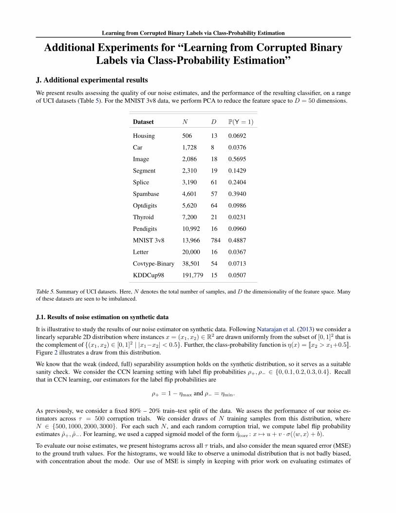
Learning from Corrupted Binary Labels via Class-Probability Estimation
Additional Experiments for “Learning from Corrupted BinaryLabels via Class-Probability Estimation”
J. Additional experimental resultsWe present results assessing the quality of our noise estimates, and the performance of the resulting classifier, on a rangeof UCI datasets (Table 5). For the MNIST 3v8 data, we perform PCA to reduce the feature space to D = 50 dimensions.
Dataset N D P(Y = 1)
Housing 506 13 0.0692
Car 1,728 8 0.0376
Image 2,086 18 0.5695
Segment 2,310 19 0.1429
Splice 3,190 61 0.2404
Spambase 4,601 57 0.3940
Optdigits 5,620 64 0.0986
Thyroid 7,200 21 0.0231
Pendigits 10,992 16 0.0960
MNIST 3v8 13,966 784 0.4887
Letter 20,000 16 0.0367
Covtype-Binary 38,501 54 0.0713
KDDCup98 191,779 15 0.0507
Table 5. Summary of UCI datasets. Here, N denotes the total number of samples, and D the dimensionality of the feature space. Manyof these datasets are seen to be imbalanced.
J.1. Results of noise estimation on synthetic data
It is illustrative to study the results of our noise estimator on synthetic data. Following Natarajan et al. (2013) we consider alinearly separable 2D distribution where instances x = (x1, x2) ∈ R2 are drawn uniformly from the subset of [0, 1]2 that isthe complement of {(x1, x2) ∈ [0, 1]2 | |x1−x2| < 0.5}. Further, the class-probability function is η(x) = Jx2 > x1+0.5K.Figure 2 illustrates a draw from this distribution.
We know that the weak (indeed, full) separability assumption holds on the synthetic distribution, so it serves as a suitablesanity check. We consider the CCN learning setting with label flip probabilities ρ+, ρ− ∈ {0, 0.1, 0.2, 0.3, 0.4}. Recallthat in CCN learning, our estimators for the label flip probabilities are
ρ+ = 1− ηmax and ρ− = ηmin.
As previously, we consider a fixed 80% – 20% train–test split of the data. We assess the performance of our noise es-timators across τ = 500 corruption trials. We consider draws of N training samples from this distribution, whereN ∈ {500, 1000, 2000, 3000}. For each such N , and each random corruption trial, we compute label flip probabilityestimates ρ+, ρ−. For learning, we used a capped sigmoid model of the form ηcorr : x 7→ u+ v · σ(〈w, x〉+ b).
To evaluate our noise estimates, we present histograms across all τ trials, and also consider the mean squared error (MSE)to the ground truth values. For the histograms, we would like to observe a unimodal distribution that is not badly biased,with concentration about the mode. Our use of MSE is simply in keeping with prior work on evaluating estimates of
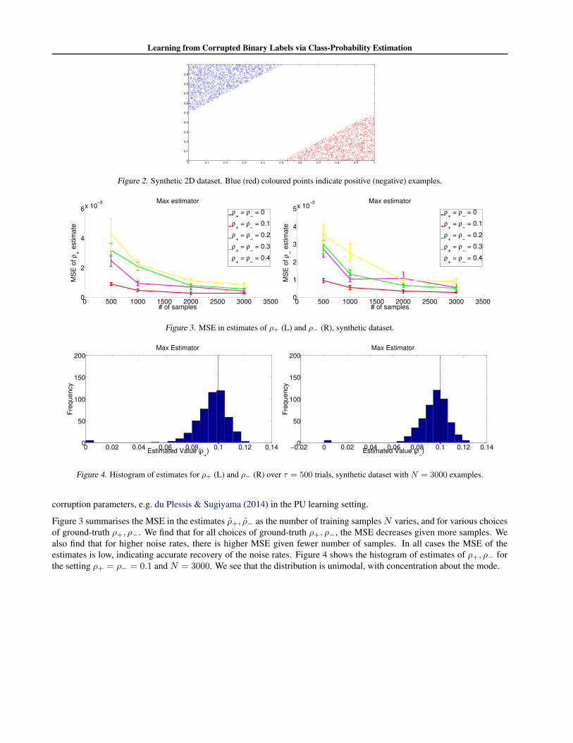
Learning from Corrupted Binary Labels via Class-Probability Estimation
0 0.1 0.2 0.3 0.4 0.5 0.6 0.7 0.8 0.9 10
0.1
0.2
0.3
0.4
0.5
0.6
0.7
0.8
0.9
1
Figure 2. Synthetic 2D dataset. Blue (red) coloured points indicate positive (negative) examples.
0 500 1000 1500 2000 2500 3000 35000
2
4
6x 10⁻³
# of samples
MS
E o
f ρ
+ e
stim
ate
Max estimator
ρ+ = ρ
− = 0
ρ+ = ρ
− = 0.1
ρ+ = ρ
− = 0.2
ρ+ = ρ
− = 0.3
ρ+ = ρ
− = 0.4
0 500 1000 1500 2000 2500 3000 35000
1
2
3
4
5x 10⁻³
# of samples
MS
E o
f ρ
− e
stim
ate
Max estimator
ρ+ = ρ
− = 0
ρ+ = ρ
− = 0.1
ρ+ = ρ
− = 0.2
ρ+ = ρ
− = 0.3
ρ+ = ρ
− = 0.4
Figure 3. MSE in estimates of ρ+ (L) and ρ− (R), synthetic dataset.
0 0.02 0.04 0.06 0.08 0.1 0.12 0.140
50
100
150
200
Estimated Value (ρ+)
Fre
qu
en
cy
Max Estimator
−0.02 0 0.02 0.04 0.06 0.08 0.1 0.12 0.140
50
100
150
200
Estimated Value (ρ−)
Fre
qu
en
cy
Max Estimator
Figure 4. Histogram of estimates for ρ+ (L) and ρ− (R) over τ = 500 trials, synthetic dataset with N = 3000 examples.
corruption parameters, e.g. du Plessis & Sugiyama (2014) in the PU learning setting.
Figure 3 summarises the MSE in the estimates ρ+, ρ− as the number of training samples N varies, and for various choicesof ground-truth ρ+, ρ−. We find that for all choices of ground-truth ρ+, ρ−, the MSE decreases given more samples. Wealso find that for higher noise rates, there is higher MSE given fewer number of samples. In all cases the MSE of theestimates is low, indicating accurate recovery of the noise rates. Figure 4 shows the histogram of estimates of ρ+, ρ− forthe setting ρ+ = ρ− = 0.1 and N = 3000. We see that the distribution is unimodal, with concentration about the mode.

Learning from Corrupted Binary Labels via Class-Probability Estimation
J.2. Violin plots of noise estimates
We present violin plots of the estimates ρ+, ρ− for all datasets and symmetric ground-truth in Figures 5 – 17. We see thatthe trend for the two quantities is largely similar. Generally, poor estimation can be attributed to either the dataset havingtoo few training examples (e.g. Car), and (or) not satisfying the weak separability assumption, as evidenced by a bias inthe estimates even in the noise-free case (e.g. Letter).
With very high noise rate (ρ+ = ρ− = 0.49), generally the bias in the estimate is low. This can be attributed to the factthat in such regimes, it is difficult to learn a discriminative classifier except with a very large number of samples.
We find that on some datasets, while there is concentration of the estimates close to the expected value, there are occa-sional outliers (e.g. Splice). These can potentially be smoothened out by some form of training set averaging, such as thebootstrap; we plan to explore this in future work.
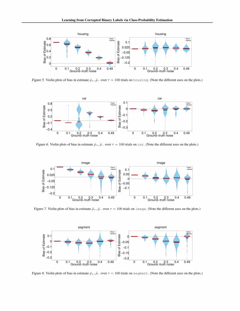
Learning from Corrupted Binary Labels via Class-Probability Estimation
0 0.1 0.2 0.3 0.4 0.49
0
0.2
0.4
0.6
0.8
Ground−truth noise
Bia
s o
f E
stim
ate
housing
MeanMedian
0 0.1 0.2 0.3 0.4 0.49
−0.2
−0.125
−0.05
0.025
0.1
Ground−truth noise
Bia
s o
f E
stim
ate
housing
MeanMedian
Figure 5. Violin plots of bias in estimate ρ+, ρ− over τ = 100 trials on housing. (Note the different axes on the plots.)
0 0.1 0.2 0.3 0.4 0.49
−0.4
−0.1
0.2
0.5
0.8
Ground−truth noise
Bia
s o
f E
stim
ate
car
Mean
Median
0 0.1 0.2 0.3 0.4 0.49
−0.3
−0.2
−0.1
0
0.1
Ground−truth noise
Bia
s o
f E
stim
ate
car
Mean
Median
Figure 6. Violin plots of bias in estimate ρ+, ρ− over τ = 100 trials on car. (Note the different axes on the plots.)
0 0.1 0.2 0.3 0.4 0.49
−0.2
−0.125
−0.05
0.025
0.1
Ground−truth noise
Bia
s o
f E
stim
ate
image
MeanMedian
0 0.1 0.2 0.3 0.4 0.49
−0.1
−0.05
0
0.05
0.1
Ground−truth noise
Bia
s o
f E
stim
ate
image
MeanMedian
Figure 7. Violin plots of bias in estimate ρ+, ρ− over τ = 100 trials on image. (Note the different axes on the plots.)
0 0.1 0.2 0.3 0.4 0.49
−0.3
−0.2
−0.1
0
0.1
Ground−truth noise
Bia
s o
f E
stim
ate
segment
MeanMedian
0 0.1 0.2 0.3 0.4 0.49−0.2
−0.15
−0.1
−0.05
0
Ground−truth noise
Bia
s o
f E
stim
ate
segment
MeanMedian
Figure 8. Violin plots of bias in estimate ρ+, ρ− over τ = 100 trials on segment. (Note the different axes on the plots.)
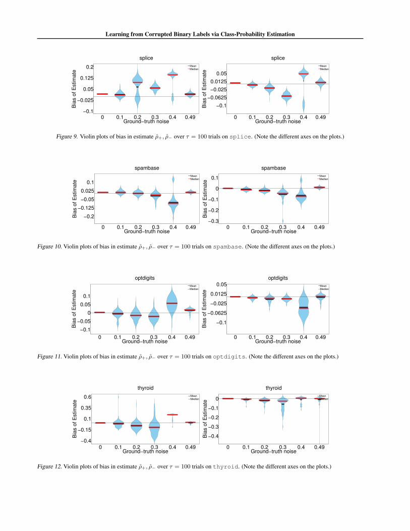
Learning from Corrupted Binary Labels via Class-Probability Estimation
0 0.1 0.2 0.3 0.4 0.49−0.1
−0.025
0.05
0.125
0.2
Ground−truth noise
Bia
s o
f E
stim
ate
splice
MeanMedian
0 0.1 0.2 0.3 0.4 0.49
−0.1
−0.0625
−0.025
0.0125
0.05
Ground−truth noise
Bia
s o
f E
stim
ate
splice
MeanMedian
Figure 9. Violin plots of bias in estimate ρ+, ρ− over τ = 100 trials on splice. (Note the different axes on the plots.)
0 0.1 0.2 0.3 0.4 0.49
−0.2
−0.125
−0.05
0.025
0.1
Ground−truth noise
Bia
s o
f E
stim
ate
spambase
MeanMedian
0 0.1 0.2 0.3 0.4 0.49−0.3
−0.2
−0.1
0
0.1
Ground−truth noise
Bia
s o
f E
stim
ate
spambase
MeanMedian
Figure 10. Violin plots of bias in estimate ρ+, ρ− over τ = 100 trials on spambase. (Note the different axes on the plots.)
0 0.1 0.2 0.3 0.4 0.49
−0.1
−0.05
0
0.05
0.1
Ground−truth noise
Bia
s o
f E
stim
ate
optdigits
MeanMedian
0 0.1 0.2 0.3 0.4 0.49
−0.1
−0.0625
−0.025
0.0125
0.05
Ground−truth noise
Bia
s o
f E
stim
ate
optdigits
MeanMedian
Figure 11. Violin plots of bias in estimate ρ+, ρ− over τ = 100 trials on optdigits. (Note the different axes on the plots.)
0 0.1 0.2 0.3 0.4 0.49−0.4
−0.15
0.1
0.35
0.6
Ground−truth noise
Bia
s o
f E
stim
ate
thyroid
MeanMedian
0 0.1 0.2 0.3 0.4 0.49
−0.4
−0.3
−0.2
−0.1
0
Ground−truth noise
Bia
s o
f E
stim
ate
thyroid
MeanMedian
Figure 12. Violin plots of bias in estimate ρ+, ρ− over τ = 100 trials on thyroid. (Note the different axes on the plots.)
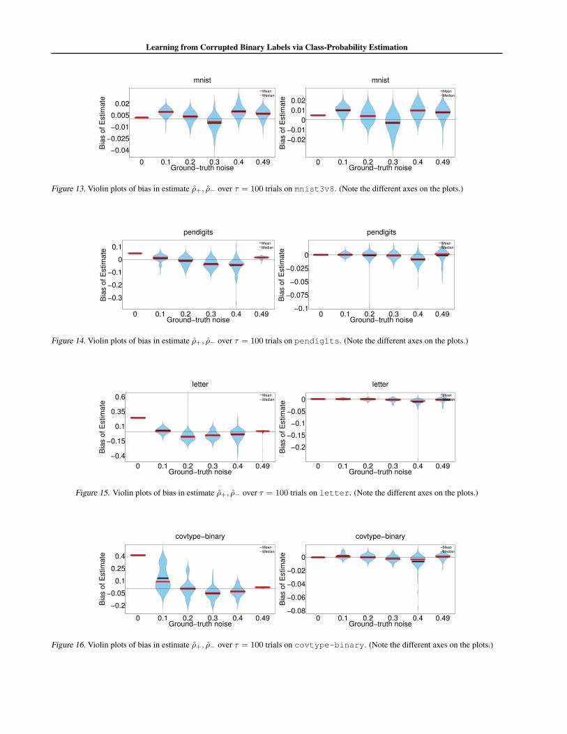
Learning from Corrupted Binary Labels via Class-Probability Estimation
0 0.1 0.2 0.3 0.4 0.49
−0.04
−0.025
−0.01
0.005
0.02
Ground−truth noise
Bia
s o
f E
stim
ate
mnist
Mean
Median
0 0.1 0.2 0.3 0.4 0.49
−0.02
−0.01
0
0.01
0.02
Ground−truth noise
Bia
s o
f E
stim
ate
mnist
Mean
Median
Figure 13. Violin plots of bias in estimate ρ+, ρ− over τ = 100 trials on mnist3v8. (Note the different axes on the plots.)
0 0.1 0.2 0.3 0.4 0.49
−0.3
−0.2
−0.1
0
0.1
Ground−truth noise
Bia
s o
f E
stim
ate
pendigits
MeanMedian
0 0.1 0.2 0.3 0.4 0.49−0.1
−0.075
−0.05
−0.025
0
Ground−truth noise
Bia
s o
f E
stim
ate
pendigits
MeanMedian
Figure 14. Violin plots of bias in estimate ρ+, ρ− over τ = 100 trials on pendigits. (Note the different axes on the plots.)
0 0.1 0.2 0.3 0.4 0.49
−0.4
−0.15
0.1
0.35
0.6
Ground−truth noise
Bia
s o
f E
stim
ate
letter
Mean
Median
0 0.1 0.2 0.3 0.4 0.49
−0.2
−0.15
−0.1
−0.05
0
Ground−truth noise
Bia
s o
f E
stim
ate
letter
Mean
Median
Figure 15. Violin plots of bias in estimate ρ+, ρ− over τ = 100 trials on letter. (Note the different axes on the plots.)
0 0.1 0.2 0.3 0.4 0.49
−0.2
−0.05
0.1
0.25
0.4
Ground−truth noise
Bia
s o
f E
stim
ate
covtype−binary
MeanMedian
0 0.1 0.2 0.3 0.4 0.49−0.08
−0.06
−0.04
−0.02
0
Ground−truth noise
Bia
s o
f E
stim
ate
covtype−binary
MeanMedian
Figure 16. Violin plots of bias in estimate ρ+, ρ− over τ = 100 trials on covtype-binary. (Note the different axes on the plots.)
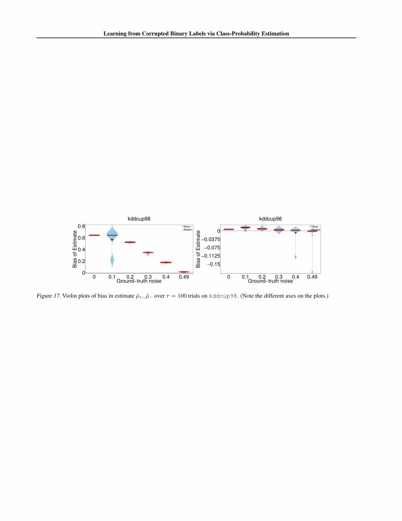
Learning from Corrupted Binary Labels via Class-Probability Estimation
0 0.1 0.2 0.3 0.4 0.490
0.2
0.4
0.6
0.8
Ground−truth noise
Bia
s o
f E
stim
ate
kddcup98
MeanMedian
0 0.1 0.2 0.3 0.4 0.49
−0.15
−0.1125
−0.075
−0.0375
0
Ground−truth noise
Bia
s o
f E
stim
ate
kddcup98
MeanMedian
Figure 17. Violin plots of bias in estimate ρ+, ρ− over τ = 100 trials on kddcup98. (Note the different axes on the plots.)
Learning from Corrupted Binary Labels via Class-Probability Estimation
J.3. Classification performance
We present results showing clean test set AUC, BER, and misclassification error for a range of noise settings in Tables 7– 16. (Recall from §7.3 that ERRmax denotes the misclassification error of the classification formed by thresholding basedon the estimated noise rates, while ERRoracle is that of the classifier formed by thresholding based on the true noise rates.)We find that generally, even with inexact estimates of ρ+, ρ−, we can attain reasonable classification performance.
Recall that the immunity of AUC and BER does not rely on the weak separability assumption. Therefore, even withimperfect performance in the noise-free case, we expect only mild degradation in general. Nonetheless, on some datasets(e.g. housing, car), there is significant degradation in the AUC and BER with moderate to high noise rates. Theseare generally accompanied by a corresponding degradation in performance of the oracle classifier. This again indicatesthat there is difficulty in accurately estimating the noisy class-conditional. One explanation for these results is that therequired sample size at moderate noise rates is not met by some of the smaller datasets. By contrast, on larger datasets, likekddcup98, we observe robustness even at high noise rates.
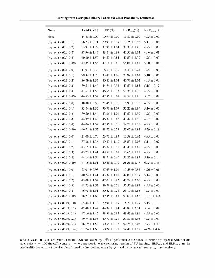
Learning from Corrupted Binary Labels via Class-Probability Estimation
Noise 1 - AUC (%) BER (%) ERRmax(%) ERRoracle(%)
None 14.48 ± 0.00 10.94 ± 0.00 19.80 ± 0.00 4.95 ± 0.00
(ρ+, ρ−) = (0.0, 0.1) 26.23 ± 0.71 29.99 ± 0.79 19.25 ± 0.96 5.11 ± 0.06
(ρ+, ρ−) = (0.0, 0.2) 33.91 ± 1.28 37.94 ± 1.04 37.30 ± 1.96 4.95 ± 0.00
(ρ+, ρ−) = (0.0, 0.3) 38.56 ± 1.45 43.84 ± 0.95 41.50 ± 1.84 4.96 ± 0.01
(ρ+, ρ−) = (0.0, 0.4) 40.30 ± 1.50 44.59 ± 0.84 49.83 ± 1.79 4.95 ± 0.00
(ρ+, ρ−) = (0.0, 0.49) 42.85 ± 1.55 47.14 ± 0.86 55.84 ± 1.81 5.00 ± 0.04
(ρ+, ρ−) = (0.1, 0.0) 17.04 ± 0.34 18.69 ± 0.70 16.39 ± 0.25 4.95 ± 0.00
(ρ+, ρ−) = (0.1, 0.1) 29.84 ± 1.20 33.45 ± 1.06 23.99 ± 1.63 5.10 ± 0.06
(ρ+, ρ−) = (0.1, 0.2) 36.89 ± 1.35 40.40 ± 1.04 40.71 ± 2.02 4.95 ± 0.00
(ρ+, ρ−) = (0.1, 0.3) 39.51 ± 1.40 44.74 ± 0.93 43.53 ± 1.85 5.15 ± 0.17
(ρ+, ρ−) = (0.1, 0.4) 41.67 ± 1.53 46.56 ± 0.73 51.38 ± 1.70 4.95 ± 0.00
(ρ+, ρ−) = (0.1, 0.49) 44.55 ± 1.57 47.86 ± 0.69 59.59 ± 1.86 5.07 ± 0.07
(ρ+, ρ−) = (0.2, 0.0) 18.88 ± 0.53 21.46 ± 0.76 15.99 ± 0.30 4.95 ± 0.00
(ρ+, ρ−) = (0.2, 0.1) 33.84 ± 1.32 36.71 ± 1.07 32.22 ± 1.99 5.16 ± 0.07
(ρ+, ρ−) = (0.2, 0.2) 39.50 ± 1.44 43.36 ± 1.01 43.57 ± 1.99 4.95 ± 0.00
(ρ+, ρ−) = (0.2, 0.3) 44.39 ± 1.48 46.37 ± 0.82 49.42 ± 1.96 4.97 ± 0.02
(ρ+, ρ−) = (0.2, 0.4) 44.06 ± 1.57 47.86 ± 0.76 54.72 ± 1.75 4.95 ± 0.00
(ρ+, ρ−) = (0.2, 0.49) 46.71 ± 1.52 48.75 ± 0.73 53.67 ± 1.92 5.29 ± 0.18
(ρ+, ρ−) = (0.3, 0.0) 21.09 ± 0.70 23.76 ± 0.93 16.59 ± 0.62 4.95 ± 0.00
(ρ+, ρ−) = (0.3, 0.1) 37.38 ± 1.36 39.89 ± 1.10 35.83 ± 2.08 5.14 ± 0.07
(ρ+, ρ−) = (0.3, 0.2) 43.15 ± 1.40 45.82 ± 0.90 49.48 ± 1.85 4.95 ± 0.00
(ρ+, ρ−) = (0.3, 0.3) 45.75 ± 1.41 48.52 ± 0.67 50.66 ± 1.91 4.95 ± 0.00
(ρ+, ρ−) = (0.3, 0.4) 44.14 ± 1.54 48.74 ± 0.60 51.22 ± 1.95 5.19 ± 0.14
(ρ+, ρ−) = (0.3, 0.49) 47.16 ± 1.51 49.46 ± 0.70 58.56 ± 1.77 6.05 ± 0.46
(ρ+, ρ−) = (0.4, 0.0) 23.01 ± 0.93 27.63 ± 1.01 17.58 ± 0.92 4.96 ± 0.01
(ρ+, ρ−) = (0.4, 0.1) 40.74 ± 1.41 43.32 ± 1.01 42.83 ± 2.19 5.14 ± 0.08
(ρ+, ρ−) = (0.4, 0.2) 45.08 ± 1.52 47.03 ± 0.82 47.74 ± 2.00 4.95 ± 0.00
(ρ+, ρ−) = (0.4, 0.3) 48.73 ± 1.53 49.79 ± 0.21 52.50 ± 1.92 4.95 ± 0.00
(ρ+, ρ−) = (0.4, 0.4) 46.95 ± 1.51 50.62 ± 0.28 55.10 ± 1.83 4.95 ± 0.00
(ρ+, ρ−) = (0.4, 0.49) 48.24 ± 1.63 49.45 ± 0.63 53.63 ± 1.82 11.78 ± 1.90
(ρ+, ρ−) = (0.49, 0.0) 25.44 ± 1.10 29.94 ± 0.99 18.77 ± 1.29 5.15 ± 0.10
(ρ+, ρ−) = (0.49, 0.1) 42.48 ± 1.47 44.39 ± 0.94 42.88 ± 2.14 5.04 ± 0.04
(ρ+, ρ−) = (0.49, 0.2) 47.16 ± 1.45 48.31 ± 0.85 48.43 ± 1.91 4.95 ± 0.00
(ρ+, ρ−) = (0.49, 0.3) 49.74 ± 1.55 49.79 ± 0.21 51.80 ± 1.93 4.95 ± 0.00
(ρ+, ρ−) = (0.49, 0.4) 46.19 ± 1.53 50.58 ± 0.37 52.74 ± 2.07 7.73 ± 1.40
(ρ+, ρ−) = (0.49, 0.49) 51.74 ± 1.60 50.24 ± 0.27 54.41 ± 1.97 44.92 ± 4.46
Table 6. Mean and standard error (standard deviation scaled by√τ ) of performance measures on housing injected with random
label noise τ = 100 times.The case ρ− = 0 corresponds to the censoring version of PU learning. ERRmax and ERRoracle are themisclassification errors of the classifiers formed by thresholding using ρ+, ρ−, and by the ground-truth ρ+, ρ− respectively.
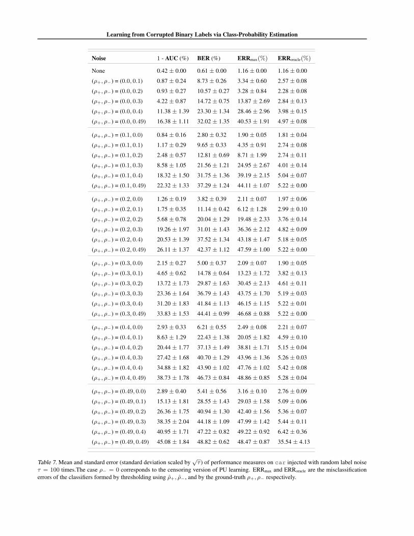
Learning from Corrupted Binary Labels via Class-Probability Estimation
Noise 1 - AUC (%) BER (%) ERRmax(%) ERRoracle(%)
None 0.42 ± 0.00 0.61 ± 0.00 1.16 ± 0.00 1.16 ± 0.00
(ρ+, ρ−) = (0.0, 0.1) 0.87 ± 0.24 8.73 ± 0.26 3.34 ± 0.60 2.57 ± 0.08
(ρ+, ρ−) = (0.0, 0.2) 0.93 ± 0.27 10.57 ± 0.27 3.28 ± 0.84 2.28 ± 0.08
(ρ+, ρ−) = (0.0, 0.3) 4.22 ± 0.87 14.72 ± 0.75 13.87 ± 2.69 2.84 ± 0.13
(ρ+, ρ−) = (0.0, 0.4) 11.38 ± 1.39 23.30 ± 1.34 28.46 ± 2.96 3.98 ± 0.15
(ρ+, ρ−) = (0.0, 0.49) 16.38 ± 1.11 32.02 ± 1.35 40.53 ± 1.91 4.97 ± 0.08
(ρ+, ρ−) = (0.1, 0.0) 0.84 ± 0.16 2.80 ± 0.32 1.90 ± 0.05 1.81 ± 0.04
(ρ+, ρ−) = (0.1, 0.1) 1.17 ± 0.29 9.65 ± 0.33 4.35 ± 0.91 2.74 ± 0.08
(ρ+, ρ−) = (0.1, 0.2) 2.48 ± 0.57 12.81 ± 0.69 8.71 ± 1.99 2.74 ± 0.11
(ρ+, ρ−) = (0.1, 0.3) 8.58 ± 1.05 21.56 ± 1.21 24.95 ± 2.67 4.01 ± 0.14
(ρ+, ρ−) = (0.1, 0.4) 18.32 ± 1.50 31.75 ± 1.36 39.19 ± 2.15 5.04 ± 0.07
(ρ+, ρ−) = (0.1, 0.49) 22.32 ± 1.33 37.29 ± 1.24 44.11 ± 1.07 5.22 ± 0.00
(ρ+, ρ−) = (0.2, 0.0) 1.26 ± 0.19 3.82 ± 0.39 2.11 ± 0.07 1.97 ± 0.06
(ρ+, ρ−) = (0.2, 0.1) 1.75 ± 0.35 11.14 ± 0.42 6.12 ± 1.28 2.99 ± 0.10
(ρ+, ρ−) = (0.2, 0.2) 5.68 ± 0.78 20.04 ± 1.29 19.48 ± 2.33 3.76 ± 0.14
(ρ+, ρ−) = (0.2, 0.3) 19.26 ± 1.97 31.01 ± 1.43 36.36 ± 2.12 4.82 ± 0.09
(ρ+, ρ−) = (0.2, 0.4) 20.53 ± 1.39 37.52 ± 1.34 43.18 ± 1.47 5.18 ± 0.05
(ρ+, ρ−) = (0.2, 0.49) 26.11 ± 1.37 42.37 ± 1.12 47.59 ± 1.00 5.22 ± 0.00
(ρ+, ρ−) = (0.3, 0.0) 2.15 ± 0.27 5.00 ± 0.37 2.09 ± 0.07 1.90 ± 0.05
(ρ+, ρ−) = (0.3, 0.1) 4.65 ± 0.62 14.78 ± 0.64 13.23 ± 1.72 3.82 ± 0.13
(ρ+, ρ−) = (0.3, 0.2) 13.72 ± 1.73 29.87 ± 1.63 30.45 ± 2.13 4.61 ± 0.11
(ρ+, ρ−) = (0.3, 0.3) 23.36 ± 1.64 36.79 ± 1.43 43.75 ± 1.70 5.19 ± 0.03
(ρ+, ρ−) = (0.3, 0.4) 31.20 ± 1.83 41.84 ± 1.13 46.15 ± 1.15 5.22 ± 0.01
(ρ+, ρ−) = (0.3, 0.49) 33.83 ± 1.53 44.41 ± 0.99 46.68 ± 0.88 5.22 ± 0.00
(ρ+, ρ−) = (0.4, 0.0) 2.93 ± 0.33 6.21 ± 0.55 2.49 ± 0.08 2.21 ± 0.07
(ρ+, ρ−) = (0.4, 0.1) 8.63 ± 1.29 22.43 ± 1.38 20.05 ± 1.82 4.59 ± 0.10
(ρ+, ρ−) = (0.4, 0.2) 20.44 ± 1.77 37.13 ± 1.49 38.81 ± 1.71 5.15 ± 0.04
(ρ+, ρ−) = (0.4, 0.3) 27.42 ± 1.68 40.70 ± 1.29 43.96 ± 1.36 5.26 ± 0.03
(ρ+, ρ−) = (0.4, 0.4) 34.88 ± 1.82 43.90 ± 1.02 47.76 ± 1.02 5.42 ± 0.08
(ρ+, ρ−) = (0.4, 0.49) 38.73 ± 1.78 46.73 ± 0.84 48.86 ± 0.85 5.28 ± 0.04
(ρ+, ρ−) = (0.49, 0.0) 2.89 ± 0.40 5.41 ± 0.56 3.16 ± 0.10 2.76 ± 0.09
(ρ+, ρ−) = (0.49, 0.1) 15.13 ± 1.81 28.55 ± 1.43 29.03 ± 1.58 5.09 ± 0.06
(ρ+, ρ−) = (0.49, 0.2) 26.36 ± 1.75 40.94 ± 1.30 42.40 ± 1.56 5.36 ± 0.07
(ρ+, ρ−) = (0.49, 0.3) 38.35 ± 2.04 44.18 ± 1.09 47.99 ± 1.42 5.44 ± 0.11
(ρ+, ρ−) = (0.49, 0.4) 40.95 ± 1.71 47.22 ± 0.82 49.22 ± 0.92 6.42 ± 0.36
(ρ+, ρ−) = (0.49, 0.49) 45.08 ± 1.84 48.82 ± 0.62 48.47 ± 0.87 35.54 ± 4.13
Table 7. Mean and standard error (standard deviation scaled by√τ ) of performance measures on car injected with random label noise
τ = 100 times.The case ρ− = 0 corresponds to the censoring version of PU learning. ERRmax and ERRoracle are the misclassificationerrors of the classifiers formed by thresholding using ρ+, ρ−, and by the ground-truth ρ+, ρ− respectively.
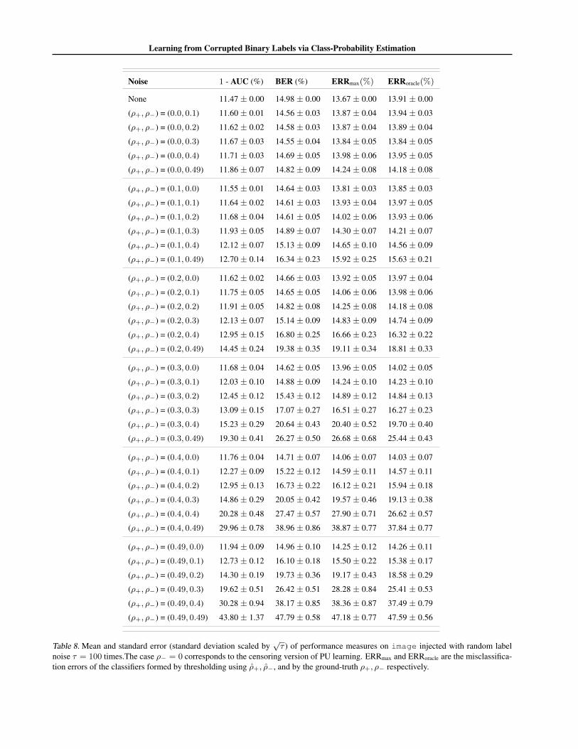
Learning from Corrupted Binary Labels via Class-Probability Estimation
Noise 1 - AUC (%) BER (%) ERRmax(%) ERRoracle(%)
None 11.47 ± 0.00 14.98 ± 0.00 13.67 ± 0.00 13.91 ± 0.00
(ρ+, ρ−) = (0.0, 0.1) 11.60 ± 0.01 14.56 ± 0.03 13.87 ± 0.04 13.94 ± 0.03
(ρ+, ρ−) = (0.0, 0.2) 11.62 ± 0.02 14.58 ± 0.03 13.87 ± 0.04 13.89 ± 0.04
(ρ+, ρ−) = (0.0, 0.3) 11.67 ± 0.03 14.55 ± 0.04 13.84 ± 0.05 13.84 ± 0.05
(ρ+, ρ−) = (0.0, 0.4) 11.71 ± 0.03 14.69 ± 0.05 13.98 ± 0.06 13.95 ± 0.05
(ρ+, ρ−) = (0.0, 0.49) 11.86 ± 0.07 14.82 ± 0.09 14.24 ± 0.08 14.18 ± 0.08
(ρ+, ρ−) = (0.1, 0.0) 11.55 ± 0.01 14.64 ± 0.03 13.81 ± 0.03 13.85 ± 0.03
(ρ+, ρ−) = (0.1, 0.1) 11.64 ± 0.02 14.61 ± 0.03 13.93 ± 0.04 13.97 ± 0.05
(ρ+, ρ−) = (0.1, 0.2) 11.68 ± 0.04 14.61 ± 0.05 14.02 ± 0.06 13.93 ± 0.06
(ρ+, ρ−) = (0.1, 0.3) 11.93 ± 0.05 14.89 ± 0.07 14.30 ± 0.07 14.21 ± 0.07
(ρ+, ρ−) = (0.1, 0.4) 12.12 ± 0.07 15.13 ± 0.09 14.65 ± 0.10 14.56 ± 0.09
(ρ+, ρ−) = (0.1, 0.49) 12.70 ± 0.14 16.34 ± 0.23 15.92 ± 0.25 15.63 ± 0.21
(ρ+, ρ−) = (0.2, 0.0) 11.62 ± 0.02 14.66 ± 0.03 13.92 ± 0.05 13.97 ± 0.04
(ρ+, ρ−) = (0.2, 0.1) 11.75 ± 0.05 14.65 ± 0.05 14.06 ± 0.06 13.98 ± 0.06
(ρ+, ρ−) = (0.2, 0.2) 11.91 ± 0.05 14.82 ± 0.08 14.25 ± 0.08 14.18 ± 0.08
(ρ+, ρ−) = (0.2, 0.3) 12.13 ± 0.07 15.14 ± 0.09 14.83 ± 0.09 14.74 ± 0.09
(ρ+, ρ−) = (0.2, 0.4) 12.95 ± 0.15 16.80 ± 0.25 16.66 ± 0.23 16.32 ± 0.22
(ρ+, ρ−) = (0.2, 0.49) 14.45 ± 0.24 19.38 ± 0.35 19.11 ± 0.34 18.81 ± 0.33
(ρ+, ρ−) = (0.3, 0.0) 11.68 ± 0.04 14.62 ± 0.05 13.96 ± 0.05 14.02 ± 0.05
(ρ+, ρ−) = (0.3, 0.1) 12.03 ± 0.10 14.88 ± 0.09 14.24 ± 0.10 14.23 ± 0.10
(ρ+, ρ−) = (0.3, 0.2) 12.45 ± 0.12 15.43 ± 0.12 14.89 ± 0.12 14.84 ± 0.13
(ρ+, ρ−) = (0.3, 0.3) 13.09 ± 0.15 17.07 ± 0.27 16.51 ± 0.27 16.27 ± 0.23
(ρ+, ρ−) = (0.3, 0.4) 15.23 ± 0.29 20.64 ± 0.43 20.40 ± 0.52 19.70 ± 0.40
(ρ+, ρ−) = (0.3, 0.49) 19.30 ± 0.41 26.27 ± 0.50 26.68 ± 0.68 25.44 ± 0.43
(ρ+, ρ−) = (0.4, 0.0) 11.76 ± 0.04 14.71 ± 0.07 14.06 ± 0.07 14.03 ± 0.07
(ρ+, ρ−) = (0.4, 0.1) 12.27 ± 0.09 15.22 ± 0.12 14.59 ± 0.11 14.57 ± 0.11
(ρ+, ρ−) = (0.4, 0.2) 12.95 ± 0.13 16.73 ± 0.22 16.12 ± 0.21 15.94 ± 0.18
(ρ+, ρ−) = (0.4, 0.3) 14.86 ± 0.29 20.05 ± 0.42 19.57 ± 0.46 19.13 ± 0.38
(ρ+, ρ−) = (0.4, 0.4) 20.28 ± 0.48 27.47 ± 0.57 27.90 ± 0.71 26.62 ± 0.57
(ρ+, ρ−) = (0.4, 0.49) 29.96 ± 0.78 38.96 ± 0.86 38.87 ± 0.77 37.84 ± 0.77
(ρ+, ρ−) = (0.49, 0.0) 11.94 ± 0.09 14.96 ± 0.10 14.25 ± 0.12 14.26 ± 0.11
(ρ+, ρ−) = (0.49, 0.1) 12.73 ± 0.12 16.10 ± 0.18 15.50 ± 0.22 15.38 ± 0.17
(ρ+, ρ−) = (0.49, 0.2) 14.30 ± 0.19 19.73 ± 0.36 19.17 ± 0.43 18.58 ± 0.29
(ρ+, ρ−) = (0.49, 0.3) 19.62 ± 0.51 26.42 ± 0.51 28.28 ± 0.84 25.41 ± 0.53
(ρ+, ρ−) = (0.49, 0.4) 30.28 ± 0.94 38.17 ± 0.85 38.36 ± 0.87 37.49 ± 0.79
(ρ+, ρ−) = (0.49, 0.49) 43.80 ± 1.37 47.79 ± 0.58 47.18 ± 0.77 47.59 ± 0.56
Table 8. Mean and standard error (standard deviation scaled by√τ ) of performance measures on image injected with random label
noise τ = 100 times.The case ρ− = 0 corresponds to the censoring version of PU learning. ERRmax and ERRoracle are the misclassifica-tion errors of the classifiers formed by thresholding using ρ+, ρ−, and by the ground-truth ρ+, ρ− respectively.

Learning from Corrupted Binary Labels via Class-Probability Estimation
Noise 1 - AUC (%) BER (%) ERRmax(%) ERRoracle(%)
None 0.00 ± 0.00 0.00 ± 0.00 0.00 ± 0.00 0.00 ± 0.00
(ρ+, ρ−) = (0.0, 0.1) 0.02 ± 0.01 0.38 ± 0.04 0.18 ± 0.03 0.18 ± 0.03
(ρ+, ρ−) = (0.0, 0.2) 0.01 ± 0.01 0.71 ± 0.07 0.23 ± 0.04 0.22 ± 0.04
(ρ+, ρ−) = (0.0, 0.3) 0.01 ± 0.01 1.08 ± 0.07 0.23 ± 0.04 0.22 ± 0.04
(ρ+, ρ−) = (0.0, 0.4) 0.02 ± 0.01 1.56 ± 0.10 0.39 ± 0.08 0.39 ± 0.08
(ρ+, ρ−) = (0.0, 0.49) 0.04 ± 0.01 2.16 ± 0.15 0.54 ± 0.08 0.50 ± 0.08
(ρ+, ρ−) = (0.1, 0.0) 0.00 ± 0.00 0.01 ± 0.00 0.01 ± 0.00 0.01 ± 0.00
(ρ+, ρ−) = (0.1, 0.1) 0.01 ± 0.00 0.46 ± 0.04 0.19 ± 0.03 0.19 ± 0.03
(ρ+, ρ−) = (0.1, 0.2) 0.02 ± 0.01 0.90 ± 0.08 0.31 ± 0.05 0.30 ± 0.05
(ρ+, ρ−) = (0.1, 0.3) 0.00 ± 0.00 1.51 ± 0.10 0.16 ± 0.04 0.16 ± 0.04
(ρ+, ρ−) = (0.1, 0.4) 0.03 ± 0.01 2.31 ± 0.16 0.47 ± 0.07 0.45 ± 0.07
(ρ+, ρ−) = (0.1, 0.49) 0.05 ± 0.01 3.15 ± 0.20 1.03 ± 0.26 0.66 ± 0.11
(ρ+, ρ−) = (0.2, 0.0) 0.00 ± 0.00 0.02 ± 0.01 0.02 ± 0.01 0.02 ± 0.01
(ρ+, ρ−) = (0.2, 0.1) 0.00 ± 0.00 0.51 ± 0.05 0.09 ± 0.02 0.10 ± 0.02
(ρ+, ρ−) = (0.2, 0.2) 0.02 ± 0.02 1.00 ± 0.08 0.18 ± 0.05 0.17 ± 0.05
(ρ+, ρ−) = (0.2, 0.3) 0.03 ± 0.01 2.00 ± 0.14 0.23 ± 0.05 0.23 ± 0.05
(ρ+, ρ−) = (0.2, 0.4) 0.03 ± 0.01 3.24 ± 0.20 0.31 ± 0.06 0.27 ± 0.06
(ρ+, ρ−) = (0.2, 0.49) 0.13 ± 0.04 5.00 ± 0.28 1.47 ± 0.25 0.94 ± 0.21
(ρ+, ρ−) = (0.3, 0.0) 0.00 ± 0.00 0.06 ± 0.02 0.06 ± 0.01 0.06 ± 0.01
(ρ+, ρ−) = (0.3, 0.1) 0.02 ± 0.01 0.60 ± 0.06 0.20 ± 0.04 0.19 ± 0.04
(ρ+, ρ−) = (0.3, 0.2) 0.03 ± 0.01 1.59 ± 0.11 0.45 ± 0.09 0.43 ± 0.08
(ρ+, ρ−) = (0.3, 0.3) 0.05 ± 0.02 2.85 ± 0.18 0.49 ± 0.09 0.45 ± 0.09
(ρ+, ρ−) = (0.3, 0.4) 0.03 ± 0.01 5.09 ± 0.27 0.62 ± 0.12 0.31 ± 0.06
(ρ+, ρ−) = (0.3, 0.49) 0.03 ± 0.01 8.41 ± 0.37 3.10 ± 0.49 1.45 ± 0.32
(ρ+, ρ−) = (0.4, 0.0) 0.01 ± 0.01 0.10 ± 0.03 0.08 ± 0.02 0.07 ± 0.02
(ρ+, ρ−) = (0.4, 0.1) 0.03 ± 0.02 0.78 ± 0.08 0.26 ± 0.07 0.24 ± 0.07
(ρ+, ρ−) = (0.4, 0.2) 0.02 ± 0.01 1.98 ± 0.15 0.23 ± 0.06 0.20 ± 0.06
(ρ+, ρ−) = (0.4, 0.3) 0.02 ± 0.01 4.24 ± 0.24 0.46 ± 0.12 0.26 ± 0.07
(ρ+, ρ−) = (0.4, 0.4) 0.07 ± 0.02 8.21 ± 0.39 3.19 ± 0.83 1.53 ± 0.33
(ρ+, ρ−) = (0.4, 0.49) 1.28 ± 0.55 16.72 ± 1.04 18.16 ± 1.87 6.80 ± 0.68
(ρ+, ρ−) = (0.49, 0.0) 0.02 ± 0.01 0.19 ± 0.06 0.17 ± 0.06 0.11 ± 0.02
(ρ+, ρ−) = (0.49, 0.1) 0.02 ± 0.01 1.00 ± 0.09 0.24 ± 0.07 0.18 ± 0.05
(ρ+, ρ−) = (0.49, 0.2) 0.05 ± 0.02 2.98 ± 0.19 0.55 ± 0.17 0.32 ± 0.08
(ρ+, ρ−) = (0.49, 0.3) 0.07 ± 0.04 6.71 ± 0.33 1.48 ± 0.43 0.48 ± 0.11
(ρ+, ρ−) = (0.49, 0.4) 5.27 ± 1.30 20.19 ± 1.51 18.16 ± 1.75 7.31 ± 0.63
(ρ+, ρ−) = (0.49, 0.49) 32.23 ± 3.17 42.82 ± 1.39 44.23 ± 1.91 31.76 ± 2.86
Table 9. Mean and standard error (standard deviation scaled by√τ ) of performance measures on segment injected with random
label noise τ = 100 times.The case ρ− = 0 corresponds to the censoring version of PU learning. ERRmax and ERRoracle are themisclassification errors of the classifiers formed by thresholding using ρ+, ρ−, and by the ground-truth ρ+, ρ− respectively.

Learning from Corrupted Binary Labels via Class-Probability Estimation
Noise 1 - AUC (%) BER (%) ERRmax(%) ERRoracle(%)
None 0.28 ± 0.00 3.40 ± 0.00 2.35 ± 0.00 2.35 ± 0.00
(ρ+, ρ−) = (0.0, 0.1) 0.76 ± 0.03 4.20 ± 0.07 3.27 ± 0.05 3.27 ± 0.05
(ρ+, ρ−) = (0.0, 0.2) 1.22 ± 0.06 4.70 ± 0.10 4.23 ± 0.09 4.23 ± 0.09
(ρ+, ρ−) = (0.0, 0.3) 1.32 ± 0.06 6.12 ± 0.12 5.04 ± 0.09 4.62 ± 0.11
(ρ+, ρ−) = (0.0, 0.4) 1.10 ± 0.04 8.85 ± 0.11 6.67 ± 0.13 4.50 ± 0.09
(ρ+, ρ−) = (0.0, 0.49) 1.46 ± 0.04 10.76 ± 0.12 9.31 ± 0.17 5.38 ± 0.10
(ρ+, ρ−) = (0.1, 0.0) 0.55 ± 0.03 4.07 ± 0.08 2.83 ± 0.06 2.79 ± 0.05
(ρ+, ρ−) = (0.1, 0.1) 1.12 ± 0.04 4.84 ± 0.09 3.75 ± 0.07 3.75 ± 0.07
(ρ+, ρ−) = (0.1, 0.2) 1.70 ± 0.07 5.79 ± 0.11 5.00 ± 0.11 4.99 ± 0.11
(ρ+, ρ−) = (0.1, 0.3) 1.48 ± 0.06 7.96 ± 0.11 6.04 ± 0.11 5.08 ± 0.10
(ρ+, ρ−) = (0.1, 0.4) 2.01 ± 0.07 10.72 ± 0.12 9.08 ± 0.18 6.19 ± 0.11
(ρ+, ρ−) = (0.1, 0.49) 3.06 ± 0.09 13.35 ± 0.14 13.53 ± 0.24 7.92 ± 0.13
(ρ+, ρ−) = (0.2, 0.0) 0.75 ± 0.03 4.95 ± 0.12 3.54 ± 0.11 3.36 ± 0.06
(ρ+, ρ−) = (0.2, 0.1) 1.60 ± 0.06 6.05 ± 0.12 4.59 ± 0.09 4.53 ± 0.08
(ρ+, ρ−) = (0.2, 0.2) 1.79 ± 0.10 7.02 ± 0.10 5.39 ± 0.16 5.56 ± 0.15
(ρ+, ρ−) = (0.2, 0.3) 2.17 ± 0.07 9.93 ± 0.14 7.75 ± 0.13 6.63 ± 0.11
(ρ+, ρ−) = (0.2, 0.4) 3.64 ± 0.13 13.29 ± 0.17 12.73 ± 0.26 9.63 ± 0.37
(ρ+, ρ−) = (0.2, 0.49) 5.09 ± 0.24 16.01 ± 0.23 18.17 ± 0.40 15.70 ± 0.59
(ρ+, ρ−) = (0.3, 0.0) 1.07 ± 0.05 5.99 ± 0.16 4.69 ± 0.22 4.09 ± 0.08
(ρ+, ρ−) = (0.3, 0.1) 1.68 ± 0.08 6.54 ± 0.12 6.37 ± 0.26 5.53 ± 0.12
(ρ+, ρ−) = (0.3, 0.2) 1.95 ± 0.06 8.75 ± 0.13 6.55 ± 0.13 6.71 ± 0.13
(ρ+, ρ−) = (0.3, 0.3) 3.68 ± 0.11 12.25 ± 0.16 10.87 ± 0.20 8.79 ± 0.16
(ρ+, ρ−) = (0.3, 0.4) 5.62 ± 0.29 16.20 ± 0.44 16.83 ± 0.39 16.14 ± 0.58
(ρ+, ρ−) = (0.3, 0.49) 12.81 ± 1.37 39.21 ± 1.43 25.62 ± 1.16 22.45 ± 0.34
(ρ+, ρ−) = (0.4, 0.0) 1.34 ± 0.08 6.67 ± 0.27 8.23 ± 0.52 5.64 ± 0.17
(ρ+, ρ−) = (0.4, 0.1) 1.59 ± 0.07 7.03 ± 0.13 8.52 ± 0.32 7.20 ± 0.14
(ρ+, ρ−) = (0.4, 0.2) 3.14 ± 0.09 10.65 ± 0.15 8.61 ± 0.15 8.70 ± 0.16
(ρ+, ρ−) = (0.4, 0.3) 6.21 ± 0.25 16.21 ± 0.55 14.99 ± 0.30 13.77 ± 0.45
(ρ+, ρ−) = (0.4, 0.4) 15.67 ± 1.52 41.24 ± 1.37 26.08 ± 1.17 22.87 ± 0.31
(ρ+, ρ−) = (0.4, 0.49) 37.37 ± 1.94 50.00 ± 0.00 42.22 ± 1.20 24.45 ± 0.00
(ρ+, ρ−) = (0.49, 0.0) 0.66 ± 0.07 4.26 ± 0.23 15.80 ± 0.40 8.84 ± 0.16
(ρ+, ρ−) = (0.49, 0.1) 2.05 ± 0.06 7.95 ± 0.13 9.68 ± 0.32 8.56 ± 0.17
(ρ+, ρ−) = (0.49, 0.2) 5.19 ± 0.15 13.49 ± 0.19 11.67 ± 0.22 11.13 ± 0.21
(ρ+, ρ−) = (0.49, 0.3) 12.57 ± 0.96 34.95 ± 1.54 23.21 ± 0.88 20.63 ± 0.44
(ρ+, ρ−) = (0.49, 0.4) 28.59 ± 1.74 49.82 ± 0.18 38.30 ± 1.20 24.48 ± 0.03
(ρ+, ρ−) = (0.49, 0.49) 48.98 ± 1.61 50.00 ± 0.00 50.33 ± 1.05 41.31 ± 2.41
Table 10. Mean and standard error (standard deviation scaled by√τ ) of performance measures on splice injected with random
label noise τ = 100 times.The case ρ− = 0 corresponds to the censoring version of PU learning. ERRmax and ERRoracle are themisclassification errors of the classifiers formed by thresholding using ρ+, ρ−, and by the ground-truth ρ+, ρ− respectively.
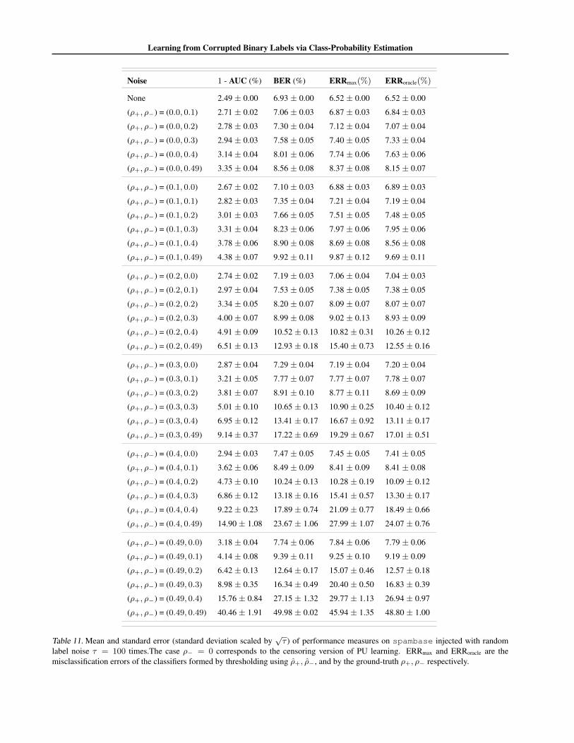
Learning from Corrupted Binary Labels via Class-Probability Estimation
Noise 1 - AUC (%) BER (%) ERRmax(%) ERRoracle(%)
None 2.49 ± 0.00 6.93 ± 0.00 6.52 ± 0.00 6.52 ± 0.00
(ρ+, ρ−) = (0.0, 0.1) 2.71 ± 0.02 7.06 ± 0.03 6.87 ± 0.03 6.84 ± 0.03
(ρ+, ρ−) = (0.0, 0.2) 2.78 ± 0.03 7.30 ± 0.04 7.12 ± 0.04 7.07 ± 0.04
(ρ+, ρ−) = (0.0, 0.3) 2.94 ± 0.03 7.58 ± 0.05 7.40 ± 0.05 7.33 ± 0.04
(ρ+, ρ−) = (0.0, 0.4) 3.14 ± 0.04 8.01 ± 0.06 7.74 ± 0.06 7.63 ± 0.06
(ρ+, ρ−) = (0.0, 0.49) 3.35 ± 0.04 8.56 ± 0.08 8.37 ± 0.08 8.15 ± 0.07
(ρ+, ρ−) = (0.1, 0.0) 2.67 ± 0.02 7.10 ± 0.03 6.88 ± 0.03 6.89 ± 0.03
(ρ+, ρ−) = (0.1, 0.1) 2.82 ± 0.03 7.35 ± 0.04 7.21 ± 0.04 7.19 ± 0.04
(ρ+, ρ−) = (0.1, 0.2) 3.01 ± 0.03 7.66 ± 0.05 7.51 ± 0.05 7.48 ± 0.05
(ρ+, ρ−) = (0.1, 0.3) 3.31 ± 0.04 8.23 ± 0.06 7.97 ± 0.06 7.95 ± 0.06
(ρ+, ρ−) = (0.1, 0.4) 3.78 ± 0.06 8.90 ± 0.08 8.69 ± 0.08 8.56 ± 0.08
(ρ+, ρ−) = (0.1, 0.49) 4.38 ± 0.07 9.92 ± 0.11 9.87 ± 0.12 9.69 ± 0.11
(ρ+, ρ−) = (0.2, 0.0) 2.74 ± 0.02 7.19 ± 0.03 7.06 ± 0.04 7.04 ± 0.03
(ρ+, ρ−) = (0.2, 0.1) 2.97 ± 0.04 7.53 ± 0.05 7.38 ± 0.05 7.38 ± 0.05
(ρ+, ρ−) = (0.2, 0.2) 3.34 ± 0.05 8.20 ± 0.07 8.09 ± 0.07 8.07 ± 0.07
(ρ+, ρ−) = (0.2, 0.3) 4.00 ± 0.07 8.99 ± 0.08 9.02 ± 0.13 8.93 ± 0.09
(ρ+, ρ−) = (0.2, 0.4) 4.91 ± 0.09 10.52 ± 0.13 10.82 ± 0.31 10.26 ± 0.12
(ρ+, ρ−) = (0.2, 0.49) 6.51 ± 0.13 12.93 ± 0.18 15.40 ± 0.73 12.55 ± 0.16
(ρ+, ρ−) = (0.3, 0.0) 2.87 ± 0.04 7.29 ± 0.04 7.19 ± 0.04 7.20 ± 0.04
(ρ+, ρ−) = (0.3, 0.1) 3.21 ± 0.05 7.77 ± 0.07 7.77 ± 0.07 7.78 ± 0.07
(ρ+, ρ−) = (0.3, 0.2) 3.81 ± 0.07 8.91 ± 0.10 8.77 ± 0.11 8.69 ± 0.09
(ρ+, ρ−) = (0.3, 0.3) 5.01 ± 0.10 10.65 ± 0.13 10.90 ± 0.25 10.40 ± 0.12
(ρ+, ρ−) = (0.3, 0.4) 6.95 ± 0.12 13.41 ± 0.17 16.67 ± 0.92 13.11 ± 0.17
(ρ+, ρ−) = (0.3, 0.49) 9.14 ± 0.37 17.22 ± 0.69 19.29 ± 0.67 17.01 ± 0.51
(ρ+, ρ−) = (0.4, 0.0) 2.94 ± 0.03 7.47 ± 0.05 7.45 ± 0.05 7.41 ± 0.05
(ρ+, ρ−) = (0.4, 0.1) 3.62 ± 0.06 8.49 ± 0.09 8.41 ± 0.09 8.41 ± 0.08
(ρ+, ρ−) = (0.4, 0.2) 4.73 ± 0.10 10.24 ± 0.13 10.28 ± 0.19 10.09 ± 0.12
(ρ+, ρ−) = (0.4, 0.3) 6.86 ± 0.12 13.18 ± 0.16 15.41 ± 0.57 13.30 ± 0.17
(ρ+, ρ−) = (0.4, 0.4) 9.22 ± 0.23 17.89 ± 0.74 21.09 ± 0.77 18.49 ± 0.66
(ρ+, ρ−) = (0.4, 0.49) 14.90 ± 1.08 23.67 ± 1.06 27.99 ± 1.07 24.07 ± 0.76
(ρ+, ρ−) = (0.49, 0.0) 3.18 ± 0.04 7.74 ± 0.06 7.84 ± 0.06 7.79 ± 0.06
(ρ+, ρ−) = (0.49, 0.1) 4.14 ± 0.08 9.39 ± 0.11 9.25 ± 0.10 9.19 ± 0.09
(ρ+, ρ−) = (0.49, 0.2) 6.42 ± 0.13 12.64 ± 0.17 15.07 ± 0.46 12.57 ± 0.18
(ρ+, ρ−) = (0.49, 0.3) 8.98 ± 0.35 16.34 ± 0.49 20.40 ± 0.50 16.83 ± 0.39
(ρ+, ρ−) = (0.49, 0.4) 15.76 ± 0.84 27.15 ± 1.32 29.77 ± 1.13 26.94 ± 0.97
(ρ+, ρ−) = (0.49, 0.49) 40.46 ± 1.91 49.98 ± 0.02 45.94 ± 1.35 48.80 ± 1.00
Table 11. Mean and standard error (standard deviation scaled by√τ ) of performance measures on spambase injected with random
label noise τ = 100 times.The case ρ− = 0 corresponds to the censoring version of PU learning. ERRmax and ERRoracle are themisclassification errors of the classifiers formed by thresholding using ρ+, ρ−, and by the ground-truth ρ+, ρ− respectively.

Learning from Corrupted Binary Labels via Class-Probability Estimation
Noise 1 - AUC (%) BER (%) ERRmax(%) ERRoracle(%)
None 0.01 ± 0.00 1.18 ± 0.00 0.18 ± 0.00 0.18 ± 0.00
(ρ+, ρ−) = (0.0, 0.1) 0.07 ± 0.01 1.04 ± 0.05 0.61 ± 0.04 0.61 ± 0.04
(ρ+, ρ−) = (0.0, 0.2) 0.11 ± 0.02 1.61 ± 0.10 0.65 ± 0.04 0.66 ± 0.04
(ρ+, ρ−) = (0.0, 0.3) 0.07 ± 0.01 2.39 ± 0.16 0.58 ± 0.05 0.58 ± 0.05
(ρ+, ρ−) = (0.0, 0.4) 0.14 ± 0.02 2.96 ± 0.20 0.75 ± 0.06 0.74 ± 0.06
(ρ+, ρ−) = (0.0, 0.49) 0.15 ± 0.04 4.71 ± 0.22 0.77 ± 0.09 0.73 ± 0.09
(ρ+, ρ−) = (0.1, 0.0) 0.01 ± 0.00 0.86 ± 0.04 0.22 ± 0.01 0.22 ± 0.01
(ρ+, ρ−) = (0.1, 0.1) 0.09 ± 0.02 1.30 ± 0.06 0.65 ± 0.04 0.63 ± 0.04
(ρ+, ρ−) = (0.1, 0.2) 0.10 ± 0.02 1.82 ± 0.12 0.67 ± 0.04 0.67 ± 0.04
(ρ+, ρ−) = (0.1, 0.3) 0.12 ± 0.02 2.63 ± 0.19 0.77 ± 0.06 0.76 ± 0.06
(ρ+, ρ−) = (0.1, 0.4) 0.24 ± 0.04 3.44 ± 0.24 1.14 ± 0.09 1.13 ± 0.09
(ρ+, ρ−) = (0.1, 0.49) 0.36 ± 0.09 4.91 ± 0.35 1.49 ± 0.19 1.42 ± 0.18
(ρ+, ρ−) = (0.2, 0.0) 0.07 ± 0.02 1.00 ± 0.05 0.28 ± 0.01 0.28 ± 0.01
(ρ+, ρ−) = (0.2, 0.1) 0.13 ± 0.02 1.23 ± 0.06 0.76 ± 0.05 0.76 ± 0.05
(ρ+, ρ−) = (0.2, 0.2) 0.19 ± 0.03 2.05 ± 0.15 0.84 ± 0.06 0.83 ± 0.06
(ρ+, ρ−) = (0.2, 0.3) 0.46 ± 0.09 3.05 ± 0.22 1.39 ± 0.17 1.39 ± 0.17
(ρ+, ρ−) = (0.2, 0.4) 0.71 ± 0.23 4.45 ± 0.40 2.23 ± 0.52 1.65 ± 0.19
(ρ+, ρ−) = (0.2, 0.49) 1.44 ± 0.50 8.44 ± 0.72 4.42 ± 1.01 1.97 ± 0.18
(ρ+, ρ−) = (0.3, 0.0) 0.06 ± 0.02 1.16 ± 0.05 0.29 ± 0.01 0.30 ± 0.01
(ρ+, ρ−) = (0.3, 0.1) 0.21 ± 0.03 1.72 ± 0.10 0.85 ± 0.06 0.84 ± 0.06
(ρ+, ρ−) = (0.3, 0.2) 0.35 ± 0.04 2.64 ± 0.17 1.09 ± 0.08 1.08 ± 0.08
(ρ+, ρ−) = (0.3, 0.3) 0.85 ± 0.08 2.82 ± 0.17 1.99 ± 0.11 2.00 ± 0.10
(ρ+, ρ−) = (0.3, 0.4) 1.21 ± 0.49 10.79 ± 0.71 4.58 ± 1.03 1.67 ± 0.21
(ρ+, ρ−) = (0.3, 0.49) 0.30 ± 0.10 15.39 ± 0.31 7.48 ± 0.44 2.53 ± 0.25
(ρ+, ρ−) = (0.4, 0.0) 0.15 ± 0.03 1.25 ± 0.07 0.31 ± 0.01 0.31 ± 0.01
(ρ+, ρ−) = (0.4, 0.1) 0.25 ± 0.03 2.13 ± 0.12 0.98 ± 0.07 0.97 ± 0.07
(ρ+, ρ−) = (0.4, 0.2) 0.73 ± 0.24 4.21 ± 0.38 1.88 ± 0.55 1.41 ± 0.11
(ρ+, ρ−) = (0.4, 0.3) 0.60 ± 0.19 9.48 ± 0.52 2.39 ± 0.42 1.77 ± 0.21
(ρ+, ρ−) = (0.4, 0.4) 0.26 ± 0.03 15.29 ± 0.30 7.58 ± 0.48 3.01 ± 0.28
(ρ+, ρ−) = (0.4, 0.49) 5.51 ± 1.06 25.66 ± 1.27 26.14 ± 1.07 5.72 ± 0.27
(ρ+, ρ−) = (0.49, 0.0) 0.39 ± 0.07 1.75 ± 0.11 0.42 ± 0.02 0.42 ± 0.02
(ρ+, ρ−) = (0.49, 0.1) 0.53 ± 0.07 3.05 ± 0.16 1.25 ± 0.10 1.24 ± 0.10
(ρ+, ρ−) = (0.49, 0.2) 0.60 ± 0.11 7.33 ± 0.41 1.59 ± 0.14 1.66 ± 0.14
(ρ+, ρ−) = (0.49, 0.3) 0.26 ± 0.05 14.16 ± 0.34 4.92 ± 0.32 2.75 ± 0.25
(ρ+, ρ−) = (0.49, 0.4) 6.01 ± 1.15 26.32 ± 1.35 25.86 ± 1.27 5.66 ± 0.28
(ρ+, ρ−) = (0.49, 0.49) 39.89 ± 2.97 47.32 ± 0.81 49.02 ± 1.10 21.43 ± 2.79
Table 12. Mean and standard error (standard deviation scaled by√τ ) of performance measures on optdigits injected with random
label noise τ = 100 times.The case ρ− = 0 corresponds to the censoring version of PU learning. ERRmax and ERRoracle are themisclassification errors of the classifiers formed by thresholding using ρ+, ρ−, and by the ground-truth ρ+, ρ− respectively.
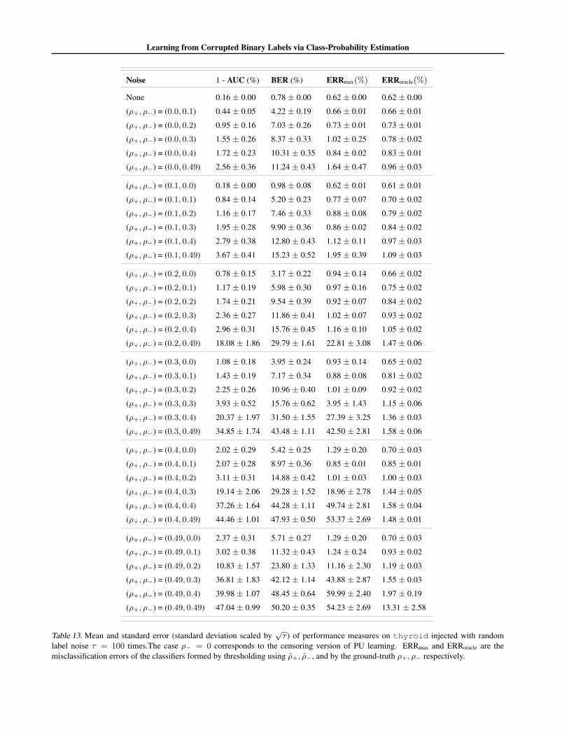
Learning from Corrupted Binary Labels via Class-Probability Estimation
Noise 1 - AUC (%) BER (%) ERRmax(%) ERRoracle(%)
None 0.16 ± 0.00 0.78 ± 0.00 0.62 ± 0.00 0.62 ± 0.00
(ρ+, ρ−) = (0.0, 0.1) 0.44 ± 0.05 4.22 ± 0.19 0.66 ± 0.01 0.66 ± 0.01
(ρ+, ρ−) = (0.0, 0.2) 0.95 ± 0.16 7.03 ± 0.26 0.73 ± 0.01 0.73 ± 0.01
(ρ+, ρ−) = (0.0, 0.3) 1.55 ± 0.26 8.37 ± 0.33 1.02 ± 0.25 0.78 ± 0.02
(ρ+, ρ−) = (0.0, 0.4) 1.72 ± 0.23 10.31 ± 0.35 0.84 ± 0.02 0.83 ± 0.01
(ρ+, ρ−) = (0.0, 0.49) 2.56 ± 0.36 11.24 ± 0.43 1.64 ± 0.47 0.96 ± 0.03
(ρ+, ρ−) = (0.1, 0.0) 0.18 ± 0.00 0.98 ± 0.08 0.62 ± 0.01 0.61 ± 0.01
(ρ+, ρ−) = (0.1, 0.1) 0.84 ± 0.14 5.20 ± 0.23 0.77 ± 0.07 0.70 ± 0.02
(ρ+, ρ−) = (0.1, 0.2) 1.16 ± 0.17 7.46 ± 0.33 0.88 ± 0.08 0.79 ± 0.02
(ρ+, ρ−) = (0.1, 0.3) 1.95 ± 0.28 9.90 ± 0.36 0.86 ± 0.02 0.84 ± 0.02
(ρ+, ρ−) = (0.1, 0.4) 2.79 ± 0.38 12.80 ± 0.43 1.12 ± 0.11 0.97 ± 0.03
(ρ+, ρ−) = (0.1, 0.49) 3.67 ± 0.41 15.23 ± 0.52 1.95 ± 0.39 1.09 ± 0.03
(ρ+, ρ−) = (0.2, 0.0) 0.78 ± 0.15 3.17 ± 0.22 0.94 ± 0.14 0.66 ± 0.02
(ρ+, ρ−) = (0.2, 0.1) 1.17 ± 0.19 5.98 ± 0.30 0.97 ± 0.16 0.75 ± 0.02
(ρ+, ρ−) = (0.2, 0.2) 1.74 ± 0.21 9.54 ± 0.39 0.92 ± 0.07 0.84 ± 0.02
(ρ+, ρ−) = (0.2, 0.3) 2.36 ± 0.27 11.86 ± 0.41 1.02 ± 0.07 0.93 ± 0.02
(ρ+, ρ−) = (0.2, 0.4) 2.96 ± 0.31 15.76 ± 0.45 1.16 ± 0.10 1.05 ± 0.02
(ρ+, ρ−) = (0.2, 0.49) 18.08 ± 1.86 29.79 ± 1.61 22.81 ± 3.08 1.47 ± 0.06
(ρ+, ρ−) = (0.3, 0.0) 1.08 ± 0.18 3.95 ± 0.24 0.93 ± 0.14 0.65 ± 0.02
(ρ+, ρ−) = (0.3, 0.1) 1.43 ± 0.19 7.17 ± 0.34 0.88 ± 0.08 0.81 ± 0.02
(ρ+, ρ−) = (0.3, 0.2) 2.25 ± 0.26 10.96 ± 0.40 1.01 ± 0.09 0.92 ± 0.02
(ρ+, ρ−) = (0.3, 0.3) 3.93 ± 0.52 15.76 ± 0.62 3.95 ± 1.43 1.15 ± 0.06
(ρ+, ρ−) = (0.3, 0.4) 20.37 ± 1.97 31.50 ± 1.55 27.39 ± 3.25 1.36 ± 0.03
(ρ+, ρ−) = (0.3, 0.49) 34.85 ± 1.74 43.48 ± 1.11 42.50 ± 2.81 1.58 ± 0.06
(ρ+, ρ−) = (0.4, 0.0) 2.02 ± 0.29 5.42 ± 0.25 1.29 ± 0.20 0.70 ± 0.03
(ρ+, ρ−) = (0.4, 0.1) 2.07 ± 0.28 8.97 ± 0.36 0.85 ± 0.01 0.85 ± 0.01
(ρ+, ρ−) = (0.4, 0.2) 3.11 ± 0.31 14.88 ± 0.42 1.01 ± 0.03 1.00 ± 0.03
(ρ+, ρ−) = (0.4, 0.3) 19.14 ± 2.06 29.28 ± 1.52 18.96 ± 2.78 1.44 ± 0.05
(ρ+, ρ−) = (0.4, 0.4) 37.26 ± 1.64 44.28 ± 1.11 49.74 ± 2.81 1.58 ± 0.04
(ρ+, ρ−) = (0.4, 0.49) 44.46 ± 1.01 47.93 ± 0.50 53.37 ± 2.69 1.48 ± 0.01
(ρ+, ρ−) = (0.49, 0.0) 2.37 ± 0.31 5.71 ± 0.27 1.29 ± 0.20 0.70 ± 0.03
(ρ+, ρ−) = (0.49, 0.1) 3.02 ± 0.38 11.32 ± 0.43 1.24 ± 0.24 0.93 ± 0.02
(ρ+, ρ−) = (0.49, 0.2) 10.83 ± 1.57 23.80 ± 1.33 11.16 ± 2.30 1.19 ± 0.03
(ρ+, ρ−) = (0.49, 0.3) 36.81 ± 1.83 42.12 ± 1.14 43.88 ± 2.87 1.55 ± 0.03
(ρ+, ρ−) = (0.49, 0.4) 39.98 ± 1.07 48.45 ± 0.64 59.99 ± 2.40 1.97 ± 0.19
(ρ+, ρ−) = (0.49, 0.49) 47.04 ± 0.99 50.20 ± 0.35 54.23 ± 2.69 13.31 ± 2.58
Table 13. Mean and standard error (standard deviation scaled by√τ ) of performance measures on thyroid injected with random
label noise τ = 100 times.The case ρ− = 0 corresponds to the censoring version of PU learning. ERRmax and ERRoracle are themisclassification errors of the classifiers formed by thresholding using ρ+, ρ−, and by the ground-truth ρ+, ρ− respectively.
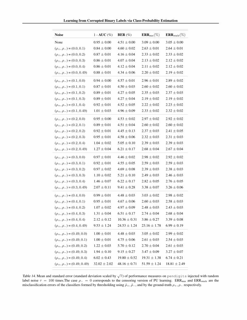
Learning from Corrupted Binary Labels via Class-Probability Estimation
Noise 1 - AUC (%) BER (%) ERRmax(%) ERRoracle(%)
None 0.95 ± 0.00 4.51 ± 0.00 3.09 ± 0.00 3.05 ± 0.00
(ρ+, ρ−) = (0.0, 0.1) 0.84 ± 0.00 4.60 ± 0.02 2.63 ± 0.01 2.64 ± 0.01
(ρ+, ρ−) = (0.0, 0.2) 0.87 ± 0.01 4.16 ± 0.04 2.33 ± 0.02 2.33 ± 0.02
(ρ+, ρ−) = (0.0, 0.3) 0.86 ± 0.01 4.07 ± 0.04 2.13 ± 0.02 2.12 ± 0.02
(ρ+, ρ−) = (0.0, 0.4) 0.86 ± 0.01 4.12 ± 0.04 2.11 ± 0.02 2.12 ± 0.02
(ρ+, ρ−) = (0.0, 0.49) 0.88 ± 0.01 4.34 ± 0.06 2.20 ± 0.02 2.19 ± 0.02
(ρ+, ρ−) = (0.1, 0.0) 0.94 ± 0.00 4.57 ± 0.01 2.96 ± 0.01 2.89 ± 0.02
(ρ+, ρ−) = (0.1, 0.1) 0.87 ± 0.01 4.50 ± 0.03 2.60 ± 0.02 2.60 ± 0.02
(ρ+, ρ−) = (0.1, 0.2) 0.89 ± 0.01 4.27 ± 0.05 2.35 ± 0.03 2.37 ± 0.03
(ρ+, ρ−) = (0.1, 0.3) 0.89 ± 0.01 4.27 ± 0.04 2.19 ± 0.02 2.19 ± 0.02
(ρ+, ρ−) = (0.1, 0.4) 0.92 ± 0.01 4.52 ± 0.05 2.22 ± 0.02 2.23 ± 0.02
(ρ+, ρ−) = (0.1, 0.49) 1.01 ± 0.03 4.96 ± 0.09 2.33 ± 0.02 2.32 ± 0.02
(ρ+, ρ−) = (0.2, 0.0) 0.95 ± 0.00 4.53 ± 0.02 2.97 ± 0.02 2.92 ± 0.02
(ρ+, ρ−) = (0.2, 0.1) 0.89 ± 0.01 4.51 ± 0.04 2.60 ± 0.02 2.60 ± 0.02
(ρ+, ρ−) = (0.2, 0.2) 0.92 ± 0.01 4.45 ± 0.13 2.37 ± 0.03 2.41 ± 0.05
(ρ+, ρ−) = (0.2, 0.3) 0.95 ± 0.01 4.58 ± 0.06 2.32 ± 0.03 2.31 ± 0.03
(ρ+, ρ−) = (0.2, 0.4) 1.04 ± 0.02 5.05 ± 0.10 2.39 ± 0.03 2.39 ± 0.03
(ρ+, ρ−) = (0.2, 0.49) 1.27 ± 0.04 6.21 ± 0.17 2.68 ± 0.04 2.67 ± 0.04
(ρ+, ρ−) = (0.3, 0.0) 0.97 ± 0.01 4.46 ± 0.02 2.98 ± 0.02 2.92 ± 0.02
(ρ+, ρ−) = (0.3, 0.1) 0.92 ± 0.01 4.55 ± 0.05 2.59 ± 0.03 2.59 ± 0.03
(ρ+, ρ−) = (0.3, 0.2) 0.97 ± 0.02 4.69 ± 0.08 2.39 ± 0.03 2.38 ± 0.03
(ρ+, ρ−) = (0.3, 0.3) 1.10 ± 0.02 5.21 ± 0.10 2.49 ± 0.03 2.46 ± 0.03
(ρ+, ρ−) = (0.3, 0.4) 1.46 ± 0.07 6.22 ± 0.17 2.82 ± 0.05 2.76 ± 0.05
(ρ+, ρ−) = (0.3, 0.49) 2.07 ± 0.11 9.41 ± 0.28 3.38 ± 0.07 3.26 ± 0.06
(ρ+, ρ−) = (0.4, 0.0) 0.99 ± 0.01 4.48 ± 0.03 3.03 ± 0.02 2.98 ± 0.02
(ρ+, ρ−) = (0.4, 0.1) 0.95 ± 0.01 4.67 ± 0.06 2.60 ± 0.03 2.58 ± 0.03
(ρ+, ρ−) = (0.4, 0.2) 1.07 ± 0.02 4.97 ± 0.09 2.48 ± 0.03 2.43 ± 0.03
(ρ+, ρ−) = (0.4, 0.3) 1.31 ± 0.04 6.51 ± 0.17 2.74 ± 0.04 2.68 ± 0.04
(ρ+, ρ−) = (0.4, 0.4) 2.12 ± 0.12 10.36 ± 0.31 3.86 ± 0.27 3.39 ± 0.08
(ρ+, ρ−) = (0.4, 0.49) 9.53 ± 1.24 24.53 ± 1.24 23.16 ± 1.78 6.99 ± 0.19
(ρ+, ρ−) = (0.49, 0.0) 1.00 ± 0.01 4.48 ± 0.03 3.05 ± 0.02 2.99 ± 0.02
(ρ+, ρ−) = (0.49, 0.1) 1.00 ± 0.01 4.75 ± 0.06 2.61 ± 0.03 2.54 ± 0.03
(ρ+, ρ−) = (0.49, 0.2) 1.22 ± 0.03 5.70 ± 0.12 2.70 ± 0.04 2.61 ± 0.03
(ρ+, ρ−) = (0.49, 0.3) 1.94 ± 0.10 9.15 ± 0.27 3.47 ± 0.09 3.27 ± 0.07
(ρ+, ρ−) = (0.49, 0.4) 6.02 ± 0.43 19.80 ± 0.52 19.31 ± 1.38 6.74 ± 0.21
(ρ+, ρ−) = (0.49, 0.49) 32.02 ± 2.02 48.16 ± 0.71 51.59 ± 1.24 18.81 ± 2.49
Table 14. Mean and standard error (standard deviation scaled by√τ ) of performance measures on pendigits injected with random
label noise τ = 100 times.The case ρ− = 0 corresponds to the censoring version of PU learning. ERRmax and ERRoracle are themisclassification errors of the classifiers formed by thresholding using ρ+, ρ−, and by the ground-truth ρ+, ρ− respectively.

Learning from Corrupted Binary Labels via Class-Probability Estimation
Noise 1 - AUC (%) BER (%) ERRmax(%) ERRoracle(%)
None 0.92 ± 0.00 3.63 ± 0.00 3.63 ± 0.00 3.63 ± 0.00
(ρ+, ρ−) = (0.0, 0.1) 0.93 ± 0.00 3.61 ± 0.01 3.59 ± 0.01 3.60 ± 0.01
(ρ+, ρ−) = (0.0, 0.2) 0.94 ± 0.01 3.63 ± 0.01 3.62 ± 0.01 3.62 ± 0.01
(ρ+, ρ−) = (0.0, 0.3) 0.96 ± 0.01 3.65 ± 0.01 3.63 ± 0.01 3.64 ± 0.01
(ρ+, ρ−) = (0.0, 0.4) 0.99 ± 0.01 3.65 ± 0.02 3.65 ± 0.02 3.66 ± 0.02
(ρ+, ρ−) = (0.0, 0.49) 1.00 ± 0.01 3.69 ± 0.02 3.68 ± 0.02 3.68 ± 0.02
(ρ+, ρ−) = (0.1, 0.0) 0.95 ± 0.01 3.56 ± 0.01 3.55 ± 0.01 3.55 ± 0.01
(ρ+, ρ−) = (0.1, 0.1) 0.96 ± 0.01 3.62 ± 0.01 3.61 ± 0.01 3.61 ± 0.01
(ρ+, ρ−) = (0.1, 0.2) 0.97 ± 0.01 3.63 ± 0.02 3.62 ± 0.02 3.62 ± 0.02
(ρ+, ρ−) = (0.1, 0.3) 1.00 ± 0.01 3.68 ± 0.02 3.67 ± 0.02 3.67 ± 0.02
(ρ+, ρ−) = (0.1, 0.4) 1.05 ± 0.01 3.78 ± 0.02 3.77 ± 0.02 3.78 ± 0.02
(ρ+, ρ−) = (0.1, 0.49) 1.10 ± 0.01 3.94 ± 0.03 3.94 ± 0.03 3.94 ± 0.03
(ρ+, ρ−) = (0.2, 0.0) 0.96 ± 0.01 3.60 ± 0.01 3.59 ± 0.01 3.59 ± 0.01
(ρ+, ρ−) = (0.2, 0.1) 0.98 ± 0.01 3.64 ± 0.02 3.63 ± 0.02 3.64 ± 0.02
(ρ+, ρ−) = (0.2, 0.2) 1.02 ± 0.01 3.67 ± 0.02 3.68 ± 0.02 3.67 ± 0.02
(ρ+, ρ−) = (0.2, 0.3) 1.07 ± 0.02 3.83 ± 0.02 3.82 ± 0.02 3.83 ± 0.02
(ρ+, ρ−) = (0.2, 0.4) 1.17 ± 0.02 4.06 ± 0.03 4.06 ± 0.03 4.05 ± 0.03
(ρ+, ρ−) = (0.2, 0.49) 1.33 ± 0.03 4.41 ± 0.04 4.41 ± 0.04 4.42 ± 0.04
(ρ+, ρ−) = (0.3, 0.0) 0.98 ± 0.01 3.65 ± 0.02 3.64 ± 0.02 3.64 ± 0.02
(ρ+, ρ−) = (0.3, 0.1) 1.03 ± 0.01 3.72 ± 0.02 3.73 ± 0.02 3.73 ± 0.02
(ρ+, ρ−) = (0.3, 0.2) 1.06 ± 0.02 3.80 ± 0.03 3.80 ± 0.03 3.81 ± 0.03
(ρ+, ρ−) = (0.3, 0.3) 1.15 ± 0.02 4.09 ± 0.03 4.09 ± 0.03 4.09 ± 0.03
(ρ+, ρ−) = (0.3, 0.4) 1.40 ± 0.03 4.55 ± 0.05 4.57 ± 0.05 4.54 ± 0.05
(ρ+, ρ−) = (0.3, 0.49) 1.62 ± 0.05 5.08 ± 0.07 5.12 ± 0.07 5.10 ± 0.07
(ρ+, ρ−) = (0.4, 0.0) 1.02 ± 0.01 3.69 ± 0.02 3.70 ± 0.02 3.70 ± 0.02
(ρ+, ρ−) = (0.4, 0.1) 1.06 ± 0.01 3.83 ± 0.02 3.85 ± 0.02 3.84 ± 0.02
(ρ+, ρ−) = (0.4, 0.2) 1.16 ± 0.02 4.05 ± 0.03 4.06 ± 0.03 4.05 ± 0.03
(ρ+, ρ−) = (0.4, 0.3) 1.37 ± 0.03 4.60 ± 0.04 4.63 ± 0.04 4.61 ± 0.04
(ρ+, ρ−) = (0.4, 0.4) 1.77 ± 0.05 5.44 ± 0.09 5.49 ± 0.08 5.48 ± 0.08
(ρ+, ρ−) = (0.4, 0.49) 2.82 ± 0.09 7.63 ± 0.14 7.95 ± 0.16 8.05 ± 0.16
(ρ+, ρ−) = (0.49, 0.0) 1.03 ± 0.01 3.72 ± 0.02 3.72 ± 0.02 3.72 ± 0.02
(ρ+, ρ−) = (0.49, 0.1) 1.13 ± 0.02 3.96 ± 0.03 3.98 ± 0.03 3.96 ± 0.03
(ρ+, ρ−) = (0.49, 0.2) 1.33 ± 0.02 4.47 ± 0.04 4.50 ± 0.05 4.48 ± 0.04
(ρ+, ρ−) = (0.49, 0.3) 1.63 ± 0.06 5.20 ± 0.08 5.26 ± 0.08 5.24 ± 0.08
(ρ+, ρ−) = (0.49, 0.4) 2.95 ± 0.09 7.93 ± 0.15 8.30 ± 0.18 8.15 ± 0.15
(ρ+, ρ−) = (0.49, 0.49) 19.56 ± 1.28 34.70 ± 1.60 35.45 ± 1.15 46.59 ± 0.82
Table 15. Mean and standard error (standard deviation scaled by√τ ) of performance measures on mnist injected with random label
noise τ = 100 times.The case ρ− = 0 corresponds to the censoring version of PU learning. ERRmax and ERRoracle are the misclassifica-tion errors of the classifiers formed by thresholding using ρ+, ρ−, and by the ground-truth ρ+, ρ− respectively.
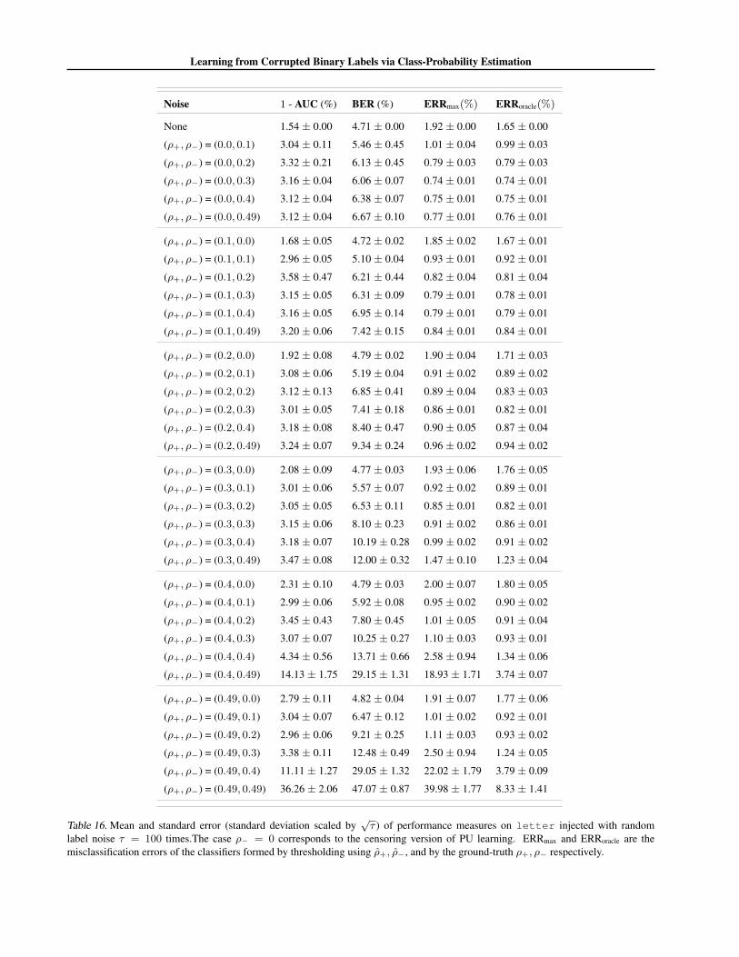
Learning from Corrupted Binary Labels via Class-Probability Estimation
Noise 1 - AUC (%) BER (%) ERRmax(%) ERRoracle(%)
None 1.54 ± 0.00 4.71 ± 0.00 1.92 ± 0.00 1.65 ± 0.00
(ρ+, ρ−) = (0.0, 0.1) 3.04 ± 0.11 5.46 ± 0.45 1.01 ± 0.04 0.99 ± 0.03
(ρ+, ρ−) = (0.0, 0.2) 3.32 ± 0.21 6.13 ± 0.45 0.79 ± 0.03 0.79 ± 0.03
(ρ+, ρ−) = (0.0, 0.3) 3.16 ± 0.04 6.06 ± 0.07 0.74 ± 0.01 0.74 ± 0.01
(ρ+, ρ−) = (0.0, 0.4) 3.12 ± 0.04 6.38 ± 0.07 0.75 ± 0.01 0.75 ± 0.01
(ρ+, ρ−) = (0.0, 0.49) 3.12 ± 0.04 6.67 ± 0.10 0.77 ± 0.01 0.76 ± 0.01
(ρ+, ρ−) = (0.1, 0.0) 1.68 ± 0.05 4.72 ± 0.02 1.85 ± 0.02 1.67 ± 0.01
(ρ+, ρ−) = (0.1, 0.1) 2.96 ± 0.05 5.10 ± 0.04 0.93 ± 0.01 0.92 ± 0.01
(ρ+, ρ−) = (0.1, 0.2) 3.58 ± 0.47 6.21 ± 0.44 0.82 ± 0.04 0.81 ± 0.04
(ρ+, ρ−) = (0.1, 0.3) 3.15 ± 0.05 6.31 ± 0.09 0.79 ± 0.01 0.78 ± 0.01
(ρ+, ρ−) = (0.1, 0.4) 3.16 ± 0.05 6.95 ± 0.14 0.79 ± 0.01 0.79 ± 0.01
(ρ+, ρ−) = (0.1, 0.49) 3.20 ± 0.06 7.42 ± 0.15 0.84 ± 0.01 0.84 ± 0.01
(ρ+, ρ−) = (0.2, 0.0) 1.92 ± 0.08 4.79 ± 0.02 1.90 ± 0.04 1.71 ± 0.03
(ρ+, ρ−) = (0.2, 0.1) 3.08 ± 0.06 5.19 ± 0.04 0.91 ± 0.02 0.89 ± 0.02
(ρ+, ρ−) = (0.2, 0.2) 3.12 ± 0.13 6.85 ± 0.41 0.89 ± 0.04 0.83 ± 0.03
(ρ+, ρ−) = (0.2, 0.3) 3.01 ± 0.05 7.41 ± 0.18 0.86 ± 0.01 0.82 ± 0.01
(ρ+, ρ−) = (0.2, 0.4) 3.18 ± 0.08 8.40 ± 0.47 0.90 ± 0.05 0.87 ± 0.04
(ρ+, ρ−) = (0.2, 0.49) 3.24 ± 0.07 9.34 ± 0.24 0.96 ± 0.02 0.94 ± 0.02
(ρ+, ρ−) = (0.3, 0.0) 2.08 ± 0.09 4.77 ± 0.03 1.93 ± 0.06 1.76 ± 0.05
(ρ+, ρ−) = (0.3, 0.1) 3.01 ± 0.06 5.57 ± 0.07 0.92 ± 0.02 0.89 ± 0.01
(ρ+, ρ−) = (0.3, 0.2) 3.05 ± 0.05 6.53 ± 0.11 0.85 ± 0.01 0.82 ± 0.01
(ρ+, ρ−) = (0.3, 0.3) 3.15 ± 0.06 8.10 ± 0.23 0.91 ± 0.02 0.86 ± 0.01
(ρ+, ρ−) = (0.3, 0.4) 3.18 ± 0.07 10.19 ± 0.28 0.99 ± 0.02 0.91 ± 0.02
(ρ+, ρ−) = (0.3, 0.49) 3.47 ± 0.08 12.00 ± 0.32 1.47 ± 0.10 1.23 ± 0.04
(ρ+, ρ−) = (0.4, 0.0) 2.31 ± 0.10 4.79 ± 0.03 2.00 ± 0.07 1.80 ± 0.05
(ρ+, ρ−) = (0.4, 0.1) 2.99 ± 0.06 5.92 ± 0.08 0.95 ± 0.02 0.90 ± 0.02
(ρ+, ρ−) = (0.4, 0.2) 3.45 ± 0.43 7.80 ± 0.45 1.01 ± 0.05 0.91 ± 0.04
(ρ+, ρ−) = (0.4, 0.3) 3.07 ± 0.07 10.25 ± 0.27 1.10 ± 0.03 0.93 ± 0.01
(ρ+, ρ−) = (0.4, 0.4) 4.34 ± 0.56 13.71 ± 0.66 2.58 ± 0.94 1.34 ± 0.06
(ρ+, ρ−) = (0.4, 0.49) 14.13 ± 1.75 29.15 ± 1.31 18.93 ± 1.71 3.74 ± 0.07
(ρ+, ρ−) = (0.49, 0.0) 2.79 ± 0.11 4.82 ± 0.04 1.91 ± 0.07 1.77 ± 0.06
(ρ+, ρ−) = (0.49, 0.1) 3.04 ± 0.07 6.47 ± 0.12 1.01 ± 0.02 0.92 ± 0.01
(ρ+, ρ−) = (0.49, 0.2) 2.96 ± 0.06 9.21 ± 0.25 1.11 ± 0.03 0.93 ± 0.02
(ρ+, ρ−) = (0.49, 0.3) 3.38 ± 0.11 12.48 ± 0.49 2.50 ± 0.94 1.24 ± 0.05
(ρ+, ρ−) = (0.49, 0.4) 11.11 ± 1.27 29.05 ± 1.32 22.02 ± 1.79 3.79 ± 0.09
(ρ+, ρ−) = (0.49, 0.49) 36.26 ± 2.06 47.07 ± 0.87 39.98 ± 1.77 8.33 ± 1.41
Table 16. Mean and standard error (standard deviation scaled by√τ ) of performance measures on letter injected with random
label noise τ = 100 times.The case ρ− = 0 corresponds to the censoring version of PU learning. ERRmax and ERRoracle are themisclassification errors of the classifiers formed by thresholding using ρ+, ρ−, and by the ground-truth ρ+, ρ− respectively.
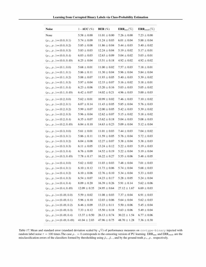
Learning from Corrupted Binary Labels via Class-Probability Estimation
Noise 1 - AUC (%) BER (%) ERRmax(%) ERRoracle(%)
None 5.58 ± 0.00 11.01 ± 0.00 7.26 ± 0.00 7.23 ± 0.00
(ρ+, ρ−) = (0.0, 0.1) 5.74 ± 0.09 11.24 ± 0.03 6.01 ± 0.04 5.88 ± 0.04
(ρ+, ρ−) = (0.0, 0.2) 5.85 ± 0.08 11.86 ± 0.04 5.44 ± 0.03 5.40 ± 0.02
(ρ+, ρ−) = (0.0, 0.3) 5.83 ± 0.03 12.24 ± 0.04 5.19 ± 0.02 5.17 ± 0.01
(ρ+, ρ−) = (0.0, 0.4) 6.03 ± 0.03 12.63 ± 0.09 5.04 ± 0.02 5.03 ± 0.01
(ρ+, ρ−) = (0.0, 0.49) 6.25 ± 0.04 13.51 ± 0.18 4.92 ± 0.02 4.92 ± 0.02
(ρ+, ρ−) = (0.1, 0.0) 5.68 ± 0.01 11.00 ± 0.02 7.57 ± 0.03 7.18 ± 0.01
(ρ+, ρ−) = (0.1, 0.1) 5.86 ± 0.11 11.30 ± 0.04 5.96 ± 0.04 5.84 ± 0.04
(ρ+, ρ−) = (0.1, 0.2) 5.88 ± 0.07 11.93 ± 0.05 5.40 ± 0.03 5.39 ± 0.02
(ρ+, ρ−) = (0.1, 0.3) 5.97 ± 0.04 12.33 ± 0.07 5.16 ± 0.02 5.18 ± 0.01
(ρ+, ρ−) = (0.1, 0.4) 6.23 ± 0.06 13.20 ± 0.16 5.03 ± 0.03 5.05 ± 0.02
(ρ+, ρ−) = (0.1, 0.49) 6.42 ± 0.07 14.02 ± 0.21 4.96 ± 0.03 5.00 ± 0.03
(ρ+, ρ−) = (0.2, 0.0) 5.62 ± 0.01 10.99 ± 0.02 7.46 ± 0.03 7.10 ± 0.02
(ρ+, ρ−) = (0.2, 0.1) 6.07 ± 0.14 11.43 ± 0.05 5.85 ± 0.04 5.76 ± 0.03
(ρ+, ρ−) = (0.2, 0.2) 5.99 ± 0.07 12.00 ± 0.05 5.42 ± 0.03 5.39 ± 0.02
(ρ+, ρ−) = (0.2, 0.3) 5.96 ± 0.04 12.62 ± 0.07 5.15 ± 0.02 5.18 ± 0.02
(ρ+, ρ−) = (0.2, 0.4) 6.35 ± 0.07 13.62 ± 0.18 5.04 ± 0.03 5.08 ± 0.03
(ρ+, ρ−) = (0.2, 0.49) 6.84 ± 0.10 14.63 ± 0.23 5.09 ± 0.04 5.12 ± 0.04
(ρ+, ρ−) = (0.3, 0.0) 5.61 ± 0.01 11.01 ± 0.03 7.44 ± 0.03 7.04 ± 0.02
(ρ+, ρ−) = (0.3, 0.1) 5.86 ± 0.11 11.59 ± 0.05 5.76 ± 0.04 5.72 ± 0.03
(ρ+, ρ−) = (0.3, 0.2) 6.04 ± 0.08 12.27 ± 0.07 5.38 ± 0.04 5.38 ± 0.03
(ρ+, ρ−) = (0.3, 0.3) 6.11 ± 0.05 13.24 ± 0.12 5.22 ± 0.03 5.19 ± 0.03
(ρ+, ρ−) = (0.3, 0.4) 6.76 ± 0.09 14.52 ± 0.19 5.22 ± 0.04 5.19 ± 0.04
(ρ+, ρ−) = (0.3, 0.49) 7.78 ± 0.17 16.22 ± 0.27 5.55 ± 0.06 5.48 ± 0.05
(ρ+, ρ−) = (0.4, 0.0) 5.62 ± 0.02 11.03 ± 0.03 7.48 ± 0.04 7.01 ± 0.03
(ρ+, ρ−) = (0.4, 0.1) 6.10 ± 0.12 11.73 ± 0.06 5.74 ± 0.04 5.68 ± 0.03
(ρ+, ρ−) = (0.4, 0.2) 6.10 ± 0.06 12.76 ± 0.10 5.34 ± 0.04 5.33 ± 0.03
(ρ+, ρ−) = (0.4, 0.3) 6.54 ± 0.07 14.23 ± 0.17 5.28 ± 0.05 5.24 ± 0.04
(ρ+, ρ−) = (0.4, 0.4) 8.09 ± 0.20 16.39 ± 0.26 5.91 ± 0.14 5.62 ± 0.06
(ρ+, ρ−) = (0.4, 0.49) 12.09 ± 0.35 24.95 ± 0.64 27.12 ± 1.67 6.69 ± 0.03
(ρ+, ρ−) = (0.49, 0.0) 5.59 ± 0.02 11.08 ± 0.03 7.37 ± 0.04 6.91 ± 0.03
(ρ+, ρ−) = (0.49, 0.1) 5.96 ± 0.10 12.03 ± 0.06 5.64 ± 0.04 5.62 ± 0.03
(ρ+, ρ−) = (0.49, 0.2) 6.46 ± 0.09 13.23 ± 0.11 5.50 ± 0.06 5.45 ± 0.04
(ρ+, ρ−) = (0.49, 0.3) 7.33 ± 0.12 15.50 ± 0.18 5.63 ± 0.06 5.49 ± 0.04
(ρ+, ρ−) = (0.49, 0.4) 13.37 ± 0.50 26.13 ± 0.74 30.22 ± 1.54 6.77 ± 0.06
(ρ+, ρ−) = (0.49, 0.49) 41.04 ± 2.03 47.96 ± 0.75 48.70 ± 1.28 7.36 ± 0.30
Table 17. Mean and standard error (standard deviation scaled by√τ ) of performance measures on covtype-binary injected with
random label noise τ = 100 times.The case ρ− = 0 corresponds to the censoring version of PU learning. ERRmax and ERRoracle are themisclassification errors of the classifiers formed by thresholding using ρ+, ρ−, and by the ground-truth ρ+, ρ− respectively.

Learning from Corrupted Binary Labels via Class-Probability Estimation
Noise 1 - AUC (%) BER (%) ERRmax(%) ERRoracle(%)
None 39.62 ± 0.00 42.46 ± 0.00 4.93 ± 0.00 4.93 ± 0.00
(ρ+, ρ−) = (0.0, 0.1) 39.91 ± 0.03 42.49 ± 0.08 9.80 ± 1.15 4.93 ± 0.00
(ρ+, ρ−) = (0.0, 0.2) 39.99 ± 0.06 42.53 ± 0.11 14.58 ± 1.92 4.93 ± 0.00
(ρ+, ρ−) = (0.0, 0.3) 39.96 ± 0.06 42.56 ± 0.08 14.37 ± 2.72 4.93 ± 0.00
(ρ+, ρ−) = (0.0, 0.4) 40.10 ± 0.06 42.70 ± 0.06 27.22 ± 8.16 4.93 ± 0.00
(ρ+, ρ−) = (0.0, 0.49) 40.15 ± 0.06 42.84 ± 0.08 21.09 ± 2.95 4.93 ± 0.00
(ρ+, ρ−) = (0.1, 0.0) 39.69 ± 0.03 42.46 ± 0.03 6.61 ± 0.66 4.93 ± 0.00
(ρ+, ρ−) = (0.1, 0.1) 39.95 ± 0.06 42.48 ± 0.07 9.38 ± 1.65 4.93 ± 0.00
(ρ+, ρ−) = (0.1, 0.2) 40.02 ± 0.07 42.54 ± 0.11 18.12 ± 1.75 4.93 ± 0.00
(ρ+, ρ−) = (0.1, 0.3) 40.02 ± 0.09 42.55 ± 0.06 15.87 ± 2.80 4.93 ± 0.00
(ρ+, ρ−) = (0.1, 0.4) 40.21 ± 0.07 42.82 ± 0.10 29.50 ± 8.24 4.93 ± 0.00
(ρ+, ρ−) = (0.1, 0.49) 40.23 ± 0.09 42.93 ± 0.11 26.25 ± 2.71 4.93 ± 0.00
(ρ+, ρ−) = (0.2, 0.0) 39.69 ± 0.03 42.39 ± 0.02 6.23 ± 0.66 4.93 ± 0.00
(ρ+, ρ−) = (0.2, 0.1) 39.95 ± 0.04 42.49 ± 0.09 15.03 ± 2.16 4.93 ± 0.00
(ρ+, ρ−) = (0.2, 0.2) 40.04 ± 0.08 42.63 ± 0.11 19.19 ± 1.62 4.93 ± 0.00
(ρ+, ρ−) = (0.2, 0.3) 40.05 ± 0.10 42.61 ± 0.10 17.60 ± 2.82 4.93 ± 0.00
(ρ+, ρ−) = (0.2, 0.4) 40.42 ± 0.11 43.01 ± 0.10 30.41 ± 8.32 4.93 ± 0.00
(ρ+, ρ−) = (0.2, 0.49) 40.44 ± 0.12 43.40 ± 0.17 32.37 ± 5.50 4.93 ± 0.00
(ρ+, ρ−) = (0.3, 0.0) 39.77 ± 0.03 42.36 ± 0.05 7.30 ± 0.61 4.93 ± 0.00
(ρ+, ρ−) = (0.3, 0.1) 40.05 ± 0.07 42.53 ± 0.09 21.20 ± 8.22 4.93 ± 0.00
(ρ+, ρ−) = (0.3, 0.2) 40.16 ± 0.12 42.74 ± 0.13 21.55 ± 2.08 4.93 ± 0.00
(ρ+, ρ−) = (0.3, 0.3) 40.22 ± 0.13 42.79 ± 0.13 20.65 ± 3.46 4.93 ± 0.00
(ρ+, ρ−) = (0.3, 0.4) 40.63 ± 0.12 43.28 ± 0.12 33.99 ± 8.64 4.93 ± 0.00
(ρ+, ρ−) = (0.3, 0.49) 41.12 ± 0.24 44.43 ± 0.66 43.34 ± 6.98 4.93 ± 0.00
(ρ+, ρ−) = (0.4, 0.0) 39.79 ± 0.04 42.39 ± 0.05 8.47 ± 1.01 4.93 ± 0.00
(ρ+, ρ−) = (0.4, 0.1) 40.06 ± 0.06 42.61 ± 0.10 15.47 ± 2.57 4.93 ± 0.00
(ρ+, ρ−) = (0.4, 0.2) 40.24 ± 0.12 42.83 ± 0.13 23.22 ± 2.33 4.93 ± 0.00
(ρ+, ρ−) = (0.4, 0.3) 40.44 ± 0.20 43.08 ± 0.13 25.10 ± 2.55 4.93 ± 0.00
(ρ+, ρ−) = (0.4, 0.4) 41.23 ± 0.18 43.81 ± 0.16 46.38 ± 8.74 4.93 ± 0.00
(ρ+, ρ−) = (0.4, 0.49) 43.59 ± 1.18 47.74 ± 0.98 46.10 ± 7.06 4.93 ± 0.00
(ρ+, ρ−) = (0.49, 0.0) 39.83 ± 0.04 42.44 ± 0.04 9.68 ± 0.93 4.93 ± 0.00
(ρ+, ρ−) = (0.49, 0.1) 40.16 ± 0.06 42.68 ± 0.13 18.99 ± 3.78 4.93 ± 0.00
(ρ+, ρ−) = (0.49, 0.2) 40.52 ± 0.20 43.19 ± 0.22 38.06 ± 8.22 4.93 ± 0.00
(ρ+, ρ−) = (0.49, 0.3) 40.80 ± 0.26 43.40 ± 0.19 27.14 ± 4.51 4.93 ± 0.00
(ρ+, ρ−) = (0.49, 0.4) 41.87 ± 0.41 44.37 ± 0.25 58.90 ± 9.60 4.93 ± 0.00
(ρ+, ρ−) = (0.49, 0.49) 49.83 ± 2.09 48.93 ± 1.05 47.44 ± 9.51 5.79 ± 0.84
Table 18. Mean and standard error (standard deviation scaled by√τ ) of performance measures on kddcup98 injected with random
label noise τ = 100 times.The case ρ− = 0 corresponds to the censoring version of PU learning. ERRmax and ERRoracle are themisclassification errors of the classifiers formed by thresholding using ρ+, ρ−, and by the ground-truth ρ+, ρ− respectively.


![[CREATING LABELS] MAKING TEXT DESIGNING LABELS … · [CREATING LABELS] MAKING TEXT DESIGNING LABELS PRINTING LABELS COMPLETED LABELS USEFUL FUNCTIONS USER'S GUIDE / Español Printed](https://img.dokumen.tips/doc/110x75/5e718e59f26dfc19d238892e/creating-labels-making-text-designing-labels-creating-labels-making-text-designing.jpg)


![Random Exemplar Hashing - GitHub Pages · hashing (STH) proposed by Zhang et al. [38]. They treat binary codes of training data as binary class labels and try to learn a set of binary](https://img.dokumen.tips/doc/110x75/5f2084d53385761339606565/random-exemplar-hashing-github-pages-hashing-sth-proposed-by-zhang-et-al-38.jpg)