Learning Chaotic Attractors by Neural Networks Chaotic Attractors by Neural Networks Rembrandt Bakker DelftChemTech, Delft University of Technology, 2628 BL Delft, The Netherlands

LETTER Communicated by Jose Principe

Learning Chaotic Attractors by Neural Networks

Rembrandt BakkerDelftChemTech Delft University of Technology 2628 BL Delft The Netherlands

Jaap C SchoutenChemical Reactor Engineering Eindhoven University of Technology 5600 MB Eind-hoven The Netherlands

C Lee GilesNEC Research Institute Princeton NJ 08540 USA

Floris TakensDepartmentof MathematicsUniversityof Groningen 9700AV Groningen The Nether-lands

Cor M van den BleekDelftChemTech Delft University of Technology5600 MB Eindhoven The Netherlands

An algorithm is introduced that trains a neural network to identify chaoticdynamics from a single measured time series During training the algo-rithm learns to short-term predict the time series At the same time acriterion developed by Diks van Zwet Takens and de Goede (1996) ismonitored that tests the hypothesis that the reconstructed attractors ofmodel-generated and measured data are the same Training is stoppedwhen the prediction error is low and the model passes this test Two otherfeatures of the algorithm are (1) the way the state of the system consist-ing of delays from the time series has its dimension reduced by weightedprincipal component analysis data reduction and (2) the user-adjustableprediction horizon obtained by ldquoerror propagationrdquomdashpartially propagat-ing prediction errors to the next time step

The algorithm is rst applied to data from an experimental-drivenchaotic pendulum of which two of the three state variables are knownThis is a comprehensive example that shows how well the Diks testcan distinguish between slightly different attractors Second the algo-rithm is applied to the same problem but now one of the two knownstate variables is ignored Finally we present a model for the laser datafrom the Santa Fe time-series competition (set A) It is the rst modelfor these data that is not only useful for short-term predictions but alsogenerates time series with similar chaotic characteristics as the measureddata

Neural Computation 12 2355ndash2383 (2000) cdeg 2000 Massachusetts Institute of Technology

2356 R Bakker J C Schouten C L Giles F Takens and C M van den Bleek

1 Introduction

A time series measured from a deterministic chaotic system has the ap-pealing characteristic that its evolution is fully determined and yet its pre-dictability is limited due to exponential growth of errors in model or mea-surements A variety of data-driven analysis methods for this type of timeseries was collected in 1991 during the Santa Fe time-series competition(Weigend amp Gershenfeld 1994) The methods focused on either character-ization or prediction of the time series No attention was given to a thirdand much more appealing objective given the data and the assumptionthat it was produced by a deterministic chaotic system nd a set of modelequations that will produce a time series with identical chaotic character-istics having the same chaotic attractor The model could be based on rstprinciples if the system is well understood but here we assume knowl-edge of just the time series and use a neural networkndashbased black-boxmodel The choice for neural networks is inspired by the inherent stabilityof their iterated predictions as opposed to for example polynomial models(Aguirre amp Billings 1994) and local linear models (Farmer amp Sidorowich1987) Lapedes and Farber (1987) were among the rst who tried the neu-ral network approach In concise neural network jargon we formulate ourgoal train a network to learn the chaotic attractor A number of authorshave addressed this issue (Aguirre amp Billings 1994 Principe Rathie ampKuo 1992 Kuo amp Principe 1994 Deco amp Schurmann 1994 Rico-Martotilde nezKrischer Kevrekidis Kube amp Hudson 1992 Krischer et al 1993 AlbanoPassamente Hediger amp Farrell 1992) The common approach consists oftwo steps

1 Identify a model that makes accurate short-term predictions

2 Generate a long time series with the model by iterated prediction andcompare the nonlinear-dynamic characteristics of the generated timeseries with the original measured time series

Principe et al (1992) found that in many cases this approach fails themodel can make good short-term predictionsbut has not learned the chaoticattractor The method would be greatly improved if we could minimizedirectly the difference between the reconstructed attractors of the model-generated and measured data rather than minimizing prediction errorsHowever we cannot reconstruct the attractor without rst having a predic-tion model Therefore research is focused on how to optimize both steps

We highly reduce the chance of failure by integrating step 2 into step 1the model identication Rather than evaluating the model attractor aftertraining we monitor the attractor during training and introduce a new testdeveloped by Diks van Zwet Takens and de Goede (1996) as a stopping cri-terion It tests the null hypothesis that the reconstructed attractors of model-generated and measured data are the same The criterion directly measures

Learning Chaotic Attractors 2357

the distance between two attractors and a good estimate of its varianceis available We combined the stopping criterion with two special featuresthat we found very useful (1) an efcient state representation by weightedprincipal component analysis (PCA) and (2) a parameter estimation schemebased on a mixture of the output-error and equation-error method previ-ously introduced as the compromisemethod (Werbos McAvoy amp Su 1992)While Werbos et al promoted the method to be used where equation errorfails we here use it to make the prediction horizon user adjustable Themethod partially propagates errors to the next time step controlled by auser-specied error propagation parameter

In this article we present three successful applications of the algorithmFirst a neural network is trained on data from an experimental driven anddamped pendulum This system is known to have three state variables ofwhich one is measured and a second the phase of the sinusoidal drivingforce is known beforehand This experiment is used as a comprehensivevisualisation of how well the Diks test can distinguish between slightlydifferent attractors and how its performance depends on the number ofdata points Second a model is trained on the same pendulum data butthis time the information about the phase of the driving force is completelyignored Instead embedding with delays and PCA is used This experimentis a practical verication of the Takens theorem (Takens 1981) as explainedin section 3 Finally the error propagation feature of the algorithm becomesimportant in the modeling of the laser data (set A) from the 1991 SantaFe time-series prediction competition The resulting neural network modelopens new possibilities for analyzing these data because it can generatetime series up to any desired length and the Jacobian of the model can becomputed analytically at any time which makes it possible to compute theLyapunov spectrum and nd periodic solutions of the model

Section 2 gives a brief description of the two data sets that are used toexplain concepts of the algorithm throughout the article In section 3 theinput-output structure of the model is dened the state is extracted fromthe single measured time series using the method of delays followed byweighted PCA and predictions are made by a combined linear and neuralnetwork model The error propagation training is outlined in section 4and the Diks test used to detect whether the attractor of the model hasconverged to the measured one in section 5 Section 6 contains the resultsof the two different pendulum models and section 7 covers the laser datamodel Section 8 concludes with remarks on attractor learning and futuredirections

2 Data Sets

Two data sets are used to illustrate features of the algorithm data from anexperimental driven pendulum and far-infrared laser data from the 1991Santa Fe time-series competition (set A) The pendulum data are described


Figure 1 Plots of the rst 2000 samples of (a) driven pendulum and (b) SantaFe laser time series

in section 21 For the laser data we refer to the extensive description ofHubner Weiss Abraham amp Tang (1994) The rst 2048 points of the eachset are plotted in Figures 1a and 1b

21 Pendulum Data The pendulum we use is a type EM-50 pendulumproduced by Daedalon Corporation (see Blackburn Vik amp Binruo 1989 fordetails and Figure 2 for a schematic drawing) Ideally the pendulum would

Figure 2 Schematic drawing of the experimental pendulum and its drivingforce The pendulum arm can rotate around its axis the angle h is measuredDuring the measurements the frequency of the driving torque was 085 Hz


obey the following equations of motion in dimensionless form

ddt

0

h

v

w

1

A D

0

v

iexclc v iexcl sinh C a sin w

vD

1

A (21)

where h is the angle of the pendulum v its angular velocity c is a dampingconstant and (a vD w ) are the amplitude frequency and phase respec-tively of the harmonic driving torque As observed by De Korte Schoutenamp van den Bleek (1995) the real pendulum deviates from the ideal behaviorof equation 21 because of its four electromagnetic driving coils that repulsethe pendulum at certain positions (top bottom left right) However froma comparison of Poincare plots of the ideal and real pendulum by Bakkerde Korte Schouten Takens amp van den Bleek (1996) it appears that the realpendulum can be described by the same three state variables (h v w ) as theequations 21 In our setup the angle h of the pendulum is measured at anaccuracy of about 01 degree It is not a well-behaved variable for it is anangle dened only in the interval [0 2p ] and it can jump from 2p to 0 in asingle time step Therefore we construct an estimate of the angular velocityv by differencing the angle time series and removing the discontinuitiesWe call this estimate V

3 Model Structure

The experimental pendulum and FIR-laser are examplesof autonomous de-terministic and stationary systems In discrete time the evolution equationfor such systems is

ExnC1 D F(Exn) (31)

where F is a nonlinear function and Exn is the state of the system at timetn D t0 C nt and t is the sampling time In most real applications only asingle variable is measured even if the evolution of the system depends onseveral variables As Grassberger Schreiber and Schaffrath (1991) pointedout it is possible to replace the vector of ldquotruerdquo state variables by a vector thatcontains delays of the single measured variable The state vector becomes adelay vector Exn D (yniexclmC1 yn) where y is the single measured variableand m is the number of delays called embedding dimension Takens (1981)showed that this method of delays will lead to evolutions of the type ofequation 31 if we choose m cedil 2D C 1 where D is the dimension of thesystemrsquos attractor We can now use this result in two ways

1 Choose an embedding a priori by xing the delay time t and thenumber of delays This results in a nonlinear auto regressive (NAR)model structuremdashin our context referred to as a time-delay neuralnetwork


2 Do not x the embedding but create a (neural network) model struc-ture with recurrent connections that the network can use to learn anappropriate state representation during training

Although the second option employs a more exible model representa-tion (see for example the FIR network model used by Wan 1994 or thepartially recurrent network of Bulsari amp Saxen 1995) we prefer to x thestate beforehand since we do not want to mix learning of two very differ-ent things an appropriate state representation and the approximation of Fin equation 31 Bengio Simard and Frasconi (1994) showed that this mixmakes it very difcult to learn long-term dependencies while Lin HorneTins and Giles (1996) showed that this can be solved by using the NAR(X)model stucture Finally Siegelmann Horne and Giles (1997) showed thatthe NAR(X) model structure may be not as compact but is computationallyas strong as a fully connected recurrent neural network

31 Choice of Embedding The choice of the delay time t and the em-bedding m is highly empirical First we x the time window with lengthT D t (miexcl1)C 1 For a properchoice of T we consider that it is too short if thevariation within the delay vector is dominated by noise and it is longer thannecessary if it exceeds the maximum prediction horizon of the systemmdashthatis if the rst and last part of the delay vector have no correlation at all Nextwe choose the delay time t Figure 3 depicts two possible choices of t fora xed window length It is important to realize that t equals the one-step-ahead prediction horizon of our model The results of Rico-Martinez et al(1992) show that if t is chosen large (such that successive delays show littlelinear correlation) the long-term solutions of the model may be apparentlydifferent from the real system due to the very discrete nature of the modelA second argument to choose t small is that the further we predict aheadin the future the more nonlinear will be the mapping F in equation 31 Asmall delay time will require the lowest functional complexity

Choosing t (very) small introduces three potential problems

1 Since we xed the time window the delay vector becomes very longand subsequent delays will be highly correlated This we solve byreducing its dimension with PCA (see section 32)

2 The one-step prediction will be highly correlated with the most recentdelays and a linear model will already make good one-step predic-tions (see section 34) We adopt the error-propagation learning algo-rithm (see section 4) to ensure learning of nonlinear correlations

3 The time needed to compute predictions over a certain time intervalis inversely proportional to the delay time For real-time applicationstoo small a delay time will make the computation of predictions pro-hibitively time-consuming


Figure 3 Two examples of an embedding with delays applied to the pendulumtime series of Figure 1a Compared to (a) in (b) the number of delays withinthe xed time window is large there is much (linear) correlation between thedelays and the one-step prediction horizon is small

The above considerations guided us for the pendulum to the embedding ofFig 3b where t D 1 and T D m D 25

32 Principal Component Embedding The consequence of a small de-lay time in a xed time window is a large embedding dimension m frac14 Tt causing the model to have an excess number of inputs that are highly cor-related Broomhead and King (1986) proposed a very convenient way toreduce the dimension of the delay vector They called it singular systemanalysis but it is better known as PCA PCA transforms the set of delayvectors to a new set of linearly uncorrelated variables of reduced dimen-sion (see Jackson 1991 for details) The principal component vectors Ezn arecomputed from the delay vectors Exn

Ezn frac14 VTExn (31)

where V is obtained from USVT D X the singular value decompositionof the matrix X that contains the original delay vectors Exn An essentialingredient of PCA is to examine how much energy is lost for each element ofEz that is discarded For the pendulum it is found that the rst 8 components


Figure 4 Accuracy (RMSEmdashroot mean square error) of the reconstruction ofthe original delay vectors (25 delays) from the principal component vectors (8principal components) for the pendulum time series (a) nonweighted PCA(c) weighted PCA (d) weighted PCA and use of update formula equation 41The standard prole we use for weighted PCA is shown in (b)

(out of 25) explain 999 of the variance of the original data To reconstructthe original data vectors PCA takes a weighted sum of the eigenvectors ofX (the columns of V) Note that King Jones and Broomhead (1987) foundthat for large embedding dimensions principal components are essentiallyFourier coefcients and the eigenvectors are sines and cosines

In particular for the case of time-series prediction where recent delaysare more important than older delays it is important to know how well eachindividual component of the delay vector Exn can be reconstructed from EznFigure 4a shows the average reconstruction error (RMSE rootmean squarederror) for each individual delay for the pendulum example where we use 8principal components It appears that the error varies with the delay and inparticular the most recent and the oldest measurement are less accuratelyrepresented than the others This is not a surprise since the rst and last delayhave correlated neighbors only on one side Ideally one would like to putsome more weight on recent measurements than older ones Grassberger etal (1991) remarked that this seems not easy when using PCA Fortunatelythe contrary is true since we can do a weighted PCA and set the desired


accuracy of each individual delay each delay is multiplied by a weightconstant The larger this constant is the more the delay will contributeto the total variance of the data and the more accurately this delay willneed to be represented For the pendulum we tried the weight prole ofFigure 4b It puts a double weight on the most recent value to compensatefor the neighbor effect The reconstruction result is shown in Figure 4c Asexpected the reconstruction of recent delays has become more accurate

33 Updating Principal Components In equation 31 the new state ofthe system is predicted from the previous one But the method of delayshas introduced information from the past in the state of the system Sinceit is not sound to predict the past we rst predict only the new measuredvariable

ynC1 D F0 (Exn) (32)

and then update the old state Exn with the prediction ynC1 to give ExnC1 For de-lay vectors Exn D (yniexclmC1 yn) this update simply involves a shift of thetime window the oldest value of y is removed and the new predicted valuecomes in In our case of principal components Exn D Ezn the update requiresthree steps (1) reconstruct the delay vector from the principal components(2) shift the time window and (3) construct the principal components fromthe updated delay vector Fortunately these three operations can be donein a single matrix computation that we call update formula (see Bakker deKorte Schouten Takens amp van den Bleek 1997 for a derivation)

EznC1 D AEzn C EbynC1 (33)

with

Aij DmX

kD2

Viexcl1ik Vkiexcl1 jI Ebi D Viexcl1

i1 (34)

Since V is orthogonal the inverse of V simply equals its transpose Viexcl1 DVT The use of the update formula equation 33 introduces some extraloss of accuracy for it computes the new state not from the original butfrom reconstructed variables This has a consequence usually small for theaverage reconstruction error compare for the pendulum example Figures 4cto 4d

A nal important issue when using principal components as neural net-work inputs is that the principal components are usually scaled accordingto the value of their eigenvalue But the small random weights initializationfor the neural networks that we will use accounts for inputs that are scaledapproximately to zero mean and unit variance This is achieved by replacingV by its scaled version W D VS and its inverse by Wiexcl1 D (XTXW )T Notethat this does not affect reconstruction errors of the PCA compression


Figure 5 Structure of the prediction model The state is updated with a newvalue of the measured variable (update unit) then fed into the linear model andan MLP neural network to predict the next value of the measured variable

34 Prediction Model After dening the state of our experimental sys-tem we need to choose a representation of the nonlinear function F in equa-tion 21 Because we prefer to use a short delay time t the one-step-aheadprediction will be highly correlated with the most recent measurement anda linear model may already make accurate one-step-ahead predictions Achaotic system is however inherently nonlinear and therefore we add astandard multilayer perceptron (MLP) to learn the nonlinearities There aretwo reasons for using both a linear and an MLP model even though theMLP itself can represent a linear model (1) the linear model parameters canbe estimated quickly beforehand with linear least squares and (2) it is in-structive to see at an early stage of training if the neural network is learningmore than linear correlations only Figure 5 shows a schematic representa-tion of the prediction model with a neural network unit a linear modelunit and a principal component update unit

4 Training Algorithm

After setting up the structure of the model we need to nd a set of param-eters for the model such that it will have an attractor as close as possible tothat of the real system In neural network terms train the model to learnthe attractor Recall that we would like to minimize directly the discrepancybetween model and system attractor but stick to the practical training ob-jective minimize short-term prediction errors The question arises whetherthis is sufcient will the prediction model also have approximately the


same attractor as the real system Principe et al (1992) showed in an ex-perimental study that this is not always the case and some years later Kuoand Principe (1994) and also Deco and Schurmann (1994) proposed as aremedy to minimize multistep rather than just one-step-ahead predictionerrors (See Haykin amp Li 1995 and Haykin amp Principe 1998 for an overviewof these methods) This approach still minimizes prediction errors (and canstill fail) but it leaves more room for optimization as it makes the predic-tion horizon user adjustable In this study we introduce in section 41 thecompromisemethod (Werbos et al 1992) as a computationally very efcientalternative for extending the prediction horizon In section 5 we assess howbest to detect differences between chaotic attractors We will stop trainingwhen the prediction error is small and no differences between attractors canbe detected

41 Error Propagation To train a prediction model we minimize thesquared difference between the predicted and measured future values Theprediction is computed from the principal component state Ez by

OynC1 D F0 (Ezn) (41)

In section 31 we recommended choosing the delay time t small As a con-sequence the one-step-ahead prediction will be highly correlated with themost recent measurements and eventually may be dominated by noise Thiswill result in bad multistep-ahead predictions As a solution Su McAvoyand Werbos (1992) proposed to train the network with an output errormethod where the state is updated with previously predicted outputs in-stead of measured outputs They call this a pure robust method and appliedit successfully to nonautonomous nonchaotic systems For autonomoussystems applying an output error method would imply that one trainsthe model to predict the entire time series from only a single initial con-dition But chaotic systems have only a limited predictability (Bockmann1991) and this approach must fail unless the prediction horizon is limited tojust a few steps This is the multistep-ahead learning approach of Kuo andPrincipe (1994) Deco and Schurmann (1994) and Jaeger and Kantz (1996)a number of initial states are selected from the measured time series andthe prediction errors over a small prediction sequence are minimized Kuoand Principe (1994) related the length of the sequences to the largest Lya-punov exponent of the system and Deco and Schurmann (1994) also putless weight on longer-term predictions to account for the decreased pre-dictability Jaeger and Kantz (1996) address the so-called error-in-variablesproblem a standard least-squares t applied to equation 41 introduces abias in the estimated parameters because it does not account for the noisein the independent variables Ezn

We investigate a second possibility to make the training of models forchaotic systems more robust It recognizes that the decreasing predictability


of chaotic systems can alternatively be explained as a loss of informationabout the state of the system when time evolves From this point of viewthe output error method will fail to predict the entire time series from onlyan initial state because this single piece of information will be lost aftera short prediction timemdashunless additional information is supplied whilethe prediction proceeds Let us compare the mathematical formulation ofthe three methods one-step ahead multistep ahead and output error withaddition of information All cases use the same prediction equation 41They differ in how they use the update formula equation 33 The one-step-ahead approach updates each time with a new measured value

EzrnC1 D AEzr

n C EbynC1 (42)

The state is labeled Ezr because it will be used as a reference state laterin equation 49 Trajectory learning or output error learning with limitedprediction horizon uses the predicted value

EznC1 D AEzn C Eb OynC1 (43)

For the third method the addition of information must somehow nd itssource in the measured time series We propose two ways to update thestate with a mixture of the predicted and measured values The rst one is

EznC1 D AEzn C Eb[(1 iexcl g)ynC1 C g OynC1] (44)

or equivalently

EznC1 D AEzn C Eb[ynC1 C gen] (45)

where the prediction error en is dened en acute OynC1 iexcl ynC1 Equation 45 andthe illustrations in Figure 6 make clear why we call g the error propagationparameter previous prediction errors are propagated to the next time stepdepending on g that we must choose between zero and one Alternativelywe can adopt the view of Werbos et al (1992) who presented the method asa compromise between the output-error (pure-robust) and equation-errormethod Prediction errors are neither completely propagated to the nexttime step (output-error method) nor suppressed (equation-error method)but they are partially propagated to the next time step For g D 0 errorpropagation is switched off and we get equation 42 For g D 1 we havefull error propagation and we get equation 43 which will work only ifthe prediction time is small In practice we use g as a user-adjustable pa-rameter intended to optimize model performance by varying the effectiveprediction horizon For example for the laser data model in section 7 wedid ve neural network training sessions each with a different value of g


Figure 6 Three ways to make predictions (a) one-step-ahead (b) multistep-ahead and (c) compromise (partially keeping the previous error in the state ofthe model)

ranging from 0 to 09 In the appendix we analyze error propagation train-ing applied to a simple problem learning the chaotic tent map There it isfound that measurement errors will be suppressed if a good value for g ischosen but that too high a value will result in a severe bias in the estimatedparameter Multistep-ahead learning has a similar disadvantage the lengthof the prediction sequence should not be chosen too high

The error propagation equation 45 has a problem when applied to thelinear model which we often add before even starting to train the MLP (seesection 34) If we replace the prediction model 44 by a linear model

ynC1 D CExn (46)

and substitute this in equation 44 we get

EznC1 D AEzn C Eb[(1 iexclg)ynC1 C gCEzn] (47)

or

EznC1 D (A C gEbC)Ezn C Eb(1 iexcl g)ynC1 (48)

This is a linear evolution of Ez with y as an exogeneous input It is BIBO(bounded input bounded output) stable if the largest eigenvalue of thematrix A C gEbC is smaller than 1 This eigenvalue is nonlinearly dependenton g and we found many cases in practice where the evolution is stablewhen g is zero or one but not for a range of in-between values thus makingerror propagation training impossible for these values of g A good remedyis to change the method into the following improved error propagationformula

EznC1 D A[Ezrn C g(Ezn iexcl Ezr

n)] C Eb[ynC1 C gen] (49)


where the reference state Ezrn is the state obtained without error propagation

as dened in equation 42 Now stability is assessed by taking the eigenval-ues ofg(A C EbC) which areg times smaller than the eigenvalues of (A C EbC)and therefore error propagation cannot disturb the stability of the systemin the case of a linear model We prefer equation 49 over equation 45 evenif no linear model is added to the MLP

42 Optimization and Training For network training we use backprop-agation through time (BPTT) and conjugate gradient minimization BPTTis needed because a nonzero error propagation parameter introduces re-currency into the network If a linear model is used parallel to the neuralnetwork we always optimize the linear model parameters rst This makesconvergence of the MLP initially slow (the easy part has already been done)and normal later on The size of the MLPs is determined by trial and errorInstead of using ldquoearly stoppingrdquo to prevent overtting we use the Diksmonitoring curves (see section 5) to decide when to stop select exactly thenumber of iterations that yields an acceptable Diks test value and a lowprediction error on independent test data The monitoring curves are alsoused to nd a suitable value for the error propagation parameter we pickthe value that yields a curve with the least irregular behavior (see the exam-ples in sections 6 and 7) Fortunately the extra work to optimize g replacesthe search for an appropriate delay time We choose that as small as thesampling time of the measurements

In a preliminary version of the algorithm (Bakker et al 1997) the pa-rameter g was taken as an additional output of the prediction model tomake it state dependent The idea was that the training procedure wouldautomatically choose g large in regions of the embedding space where thepredictability is high and small where predictability is low We now thinkthat this gives the minimization algorithm too many degrees of freedomand we prefer simply to optimize g by hand

5 Diks Test Monitoring

Because the error propagation training does not guarantee learning of thesystem attractor we need to monitor a comparison between the model andsystem attractor Several authors have used dynamic invariants such asLyapunov exponents entropies and correlation dimension to compare at-tractors (Aguirre amp Billings 1994 Principe et al 1992 Bakker et al 1997Haykin amp Puthusserypady 1997) These invariants are certainly valuablebut they do not uniquely identify the chaotic system and their condencebounds are hard to estimate Diks et al (1996) has developed a methodthat is unique if the two attractors are the same the test value will be zerofor a sufcient number of samples The method can be seen as an objec-tive substitute for visual comparison of attractors plotted in the embedding


space The test works for low- and high-dimensional systems and unlikethe previouslymentioned invariants its variance can be well estimated fromthe measured data The following null hypothesis is tested the two sets ofdelay vectors (model generated measured) are drawn from the same multidimen-sional probability distribution The two distributions r 0

1(Er ) and r 02( Er ) are rst

smoothed using gaussian kernels resulting inr1( Er ) and r2( Er ) and then thedistance between the smoothed distributions is dened to be the volumeintegral over the squared difference between the two distributions

Q DZ

dEr(r 01( Er ) iexcl r 0

2(Er ))2 (51)

The smoothing is needed to make Q applicable to the fractal probability dis-tributions encountered in the strange attractors of chaotic systems Diks etal (1996) provide an unbiased estimate for Q and for its variance Vc wheresubscript c means ldquounder the condition that the null hypothesis holdsrdquo Inthat case the ratio S D OQ

pVc is a random variable with zero mean and unit

variance Two issues need special attention the test assumes independenceamong all vectors and the gaussian kernels use a bandwidth parameter dthat determines the length scale of the smoothing In our case the succes-sive states of the system will be very dependent due to the short predictiontime The simplest solution is to choose a large time interval between the de-lay vectorsmdashat least several embedding timesmdashand ignore what happensin between Diks et al (1996) propose a method that makes more efcientuse of the available data It divides the time series in segments of length land uses an averaging procedure such that the assumption of independentvectors can be replaced by the assumption of independent segments Thechoice of bandwidth d determines the sensitivity of the test Diks et al (1996)suggest using a small part of the available data to nd out which value ofd gives the highest test value and using this value for the nal test with thecomplete sets of data

In our practical implementation we compress the delay vectors to prin-cipal component vectors for computational efciency knowing that

kEx1 iexcl Ex2k2 frac14 kU(Ez1 iexcl Ez2)k2 D kEz1 iexcl Ez2k2 (52)

since U is orthogonal We vary the sampling interval randomly betweenone and two embedding times and use l D 4 We generate 11 independentsets with the model each with a length of two times the measured time-series length The rst set is used to nd the optimum value for d andthe other 10 sets to get an estimate of S and to verify experimentally itsstandard deviation that is supposed to be unity Diks et al (1996) suggestrejecting the null hypothesis with more than 95 condence for S gt 3 Ourestimate of S is the average of 10 evaluations Each evaluation uses new andindependent model-generated data but the same measured data (only the


Figure 7 Structure of pendulum model I that uses all available informationabout the pendulum the measured angleh the known phase of the driving forcew the estimated angular velocity V and nonlinear terms (sines and cosines) thatappear in the equations of motion equation 21

sampling is done again) To account for the 10 half-independent evaluationswe lower the 95 condence threshold to S D 3

p(12 cent 10) frac14 14 Note

that the computational complexity of the Diks test is the same as that ofcomputing correlation entropies or dimensionsmdashroughly O(N2) where Nis the number of delay vectors in the largest of the two sets to be compared

6 Modeling the Experimental Pendulum

In this chapter we present two models for the chaotic driven and dampedpendulum that was introduced in section 21 The rst model pendulummodel I uses all possible relevant inputs that is the measured angle theknown phase of the driving force and some nonlinear terms suggested bythe equations of motion of the pendulum This model does not use errorpropagation or principal component analysis it is used just to demonstratethe performance of the Diks test The second model pendulum model IIuses a minimum of different inputsmdashjust a single measured series of theestimated angular velocity V (dened in section 21) This is a practicalverication of the Takens theorem (see section 3) since we disregard twoof the three ldquotruerdquo state variables and use delays instead We will reducethe dimension of the delay vector by PCA There is no need to use errorpropagation since the data have a very low noise level

61 Pendulum Model I This model is the same as that of Bakker et al(1996) except for the external input that is notpresent here The input-outputstructure is shown in Figure 7 The network has 24 nodes in the rst and8 in the second hidden layer The network is trained by backpropagation


Figure 8 Development of the Poincare plot of pendulum model I during train-ing to be compared with the plot of measured data (a) The actual developmentis not as smooth as suggested by (bndashf) as can be seen from the Diks test moni-toring curves in Figure 9

with conjugate gradient minimization on a time series of 16000 samplesand reaches an error level for the one-step-ahead prediction of the angle has low as 027 degree on independent data The attractor of this system is theplot of the evolutions of the state vectors (V h Q)n in a three-dimensionalspace Two-dimensional projections called Poincare sections are shown inFigure 8 each time a new cycle of the sinusoidal driving force starts whenthe phase Q is zero a point (V h )n is plotted Figure 8a shows measureddata while Figures 8b through 8f show how the attractor of the neuralnetwork model evolves as training proceeds Visual inspection reveals thatthe Poincare section after 8000 conjugate gradient iterations is still slightlydifferent from the measured attractor and it is interesting to see if we woulddraw the same conclusion if we use the Diks test To enable a fair comparisonwith the pendulum model II results in the next section we compute theDiks test not directly from the states (V h Q)n (that would probably bemost powerful) but instead reconstruct the attractor in a delay space of thevariable V the onlyvariable that will be available inpendulum model II anduse these delay vectors to compute the Diks test To see how the sensitivity ofthe test depends on the length of the time series we compute it three times


Figure 9 Diks test monitoring curve for pendulum model I The Diks test con-verges to zero (no difference between model and measured attractor can befound) but the spikes indicate the extreme sensitivity of the model attractor forthe model parameters

using 1 2 and 16 data sets of 8000 points each These numbers shouldbe compared to the length of the time series used to create the Poincaresections 15 million points of which each 32nd point (when the phase Qis 0) is plotted The Diks test results are printed in the top-right corner ofeach of the graphs in Figure 8 The test based on only one set of 8000 (Diks8K) points cannot see the difference between Figures 8a and 8c whereas thetest based on all 16 sets (Diks 128K) can still distinguish between Figures 8aand 8e

It may seem from the Poincare sections in Figures 8b through 8f that themodel attractor gradually converges toward the measured attractor whentraining proceeds However from the Diks test monitoringcurve in Figure 9we can conclude that this isnotat all the case The spikes in the curve indicatethat even after the model attractor gets very close to the measured attractora complete mismatch may occur from one iteration to the other We willsee a similar behavior for the pendulum model II (see section 62) and thelaser data model (see section 7) and address the issue in the discussion (seesection 8)

62 Pendulum Model II This model uses information from just a singlevariable the estimated angular velocity V From the equations of motionequation 21 it follows that the pendulum has three state variables and theTakens theorem tells us that in the case of noise-free data an embedding of7(2 curren 3 C 1) delays will be sufcient In our practical application we take theembedding of Figure 3b with 25 delays which are reduced to 8 principalcomponents by weighted PCA The network has 24 nodes in the rst and 8in the second hidden layer and a linear model is added First the networkis trained for 4000 iterations on a train set of 8000 points then a second setof 8000 points is added and training proceeds for another 2000 iterations


reaching an error level of 074 degree two and a half times larger thanmodel I The Diks test monitoring curve (not shown) has the same irregularbehavior as for pendulum model I In between the spikes it eventuallyvaries between one and two Compare this to model I after 2000 iterationsas shown in Figure 8e which has a Diks test of 06 model II does not learnthe attractor as well as model I That is the price we pay for omitting a prioriinformation about the phase of the driving force and the nonlinear termsfrom the equations of motion

We also computed Lyapunov exponents l For model I we recall the es-timated largest exponent of 25 bits per driving cycle as found in Bakker etal (1996) For model II we computed a largest exponent of 24 bits per cycleusing the method of von Bremen et al (1997) that uses QR-factorizationsof tangent maps along model-generated trajectories The method actuallycomputes the entire Lyapunov spectrum and from that we can estimate theinformation dimension D1 of the system using the Kaplan-Yorke conjec-ture (Kaplan amp Yorke 1979) take that (real) value of i where the interpo-lated curve

Pi l i versus i crosses zero This happens at D1 D 35 with an

estimated standard deviation of 01 For comparison the ideal chaotic pen-dulum as dened by equation 21 has three exponents and as mentionedin Bakker et al (1996) the largest is positive the second zero and the sumof all three is negative This tells us that the dimension must lie between 2and 3 This means that pendulum model II has a higher dimension than thereal system We think this is because of the high embedding space (eightprincipal components) that is used Apparently the model has not learnedto make the ve extra spurious Lyapunov exponents more negative thanthe smallest exponent in the real system Eckmann Kamphorst Ruelle andCiliberto (1986) report the same problem when they model chaotic datawith local linear models We also computed an estimate for the correla-tion dimension and entropy of the time series with the computer packageRRCHAOS (Schouten amp van den Bleek 1993) which uses the maximumlikeliehood estimation procedures of Schouten Takens and van den Bleek(1994a 1994b) For the measured data we found a correlation dimensionof 31+iexcl01 and for the model-generated data 29+iexcl01 there was nosignicant difference between the two numbers but the numbers are veryclose to the theoretical maximum of three For the correlation entropy wefound 24+iexcl01 bits per cycle for measured data and 22+iexcl02 bits percycle for the model-generated data Again there was no signicant differ-ence and moreover the entropy is almost the same as the estimated largestLyapunov exponent

For pendulum model II we relied on the Diks test to compare attractorsHowever even if we do not have the phase of the driving force available aswe did in model I we can still make plots of cross-sections of the attractor byprojecting them in a two-dimensional space This is what we do in Figure 10every time when the rst state variable upwardly crosses zero we plot theremaining seven state variables in a two-dimensional projection


Figure 10 Poincare section based on measured (a) and model-generated (b)dataA series of truncatedstates (z1 z2 z3)T is reconstructed from the time seriesa point (z2 z3)T is plotted every time z1 crosses zero (upward)

7 Laser Data Model

The second application of the training algorithm is the well-known laserdata set (set A) from the Santa Fe time series competition (Weigend amp Ger-shenfeld 1994) The model is similar to that reported in Bakker SchoutenGiles amp van den Bleek (1998) but instead of using the rst 3000 pointsfor training we use only 1000 pointsmdashexactly the amount of data that wasavailable before the results of the time-series competition were publishedWe took an embedding of 40 and used PCA to reduce the 40 delays to 16principal components First a linear model was tted to make one-step-ahead predictions This already explained 80 of the output data varianceThe model was extended with an MLP having 16 inputs (the 16 principalcomponents) two hidden layers with 32 and 24 sigmoidal nodes and asingle output (the time-series value to be predicted) Five separate trainingsessions were carried out using 0 60 70 80 and 90 error prop-agation (the percentage corresponds to g cent 100) Each session lasted 4000conjugate gradient iterations and the Diks test was evaluated every 20 iter-ations Figure 11 shows the monitoring results We draw three conclusionsfrom it

1 While the prediction error on the training set (not shown) monoton-ically decreases during training the Diks test shows very irregularbehavior We saw the same irregular behavior for the two pendulummodels

2 The case of 70 error propagation converges best to a model thathas learned the attractor and does not ldquoforget the attractorrdquo whentraining proceeds The error propagation helps to suppress the noisethat is present in the time series


Figure 11 Diks test monitoring curves for the laser data model with (a) 0(b) 60 (c) 70 (d) 80 (e) 90 error propagation On the basis of these curvesit is decided to select the model trained with 70 error propagation and after1300 iterations for further analysis

3 The common stopping criterion ldquostop when error on test set is at itsminimumrdquo may yield a model with an unacceptable Diks test resultInstead we have to monitor the Diks test carefully and select exactlythat model that has both a low prediction error and a good attractormdasha low Diks test value that does not change from one iteration to theother

Experience has shown that the Diks test result of each training sessionis sensitive for the initial weights of the MLP the curves are not well re-producible Trial and error is required For example in Bakker et al (1998)where we used more training data to model the laser we selected 90 errorpropagation (EP) to be the best choice by looking at the Diks test monitoringcurves

For further analysis we select the model trained with 70 EP after 1300iterations having a Diks test value averaged over 100 iterations as lowas iexcl02 Figure 12b shows a time series generated by this model alongwith measured data For the rst 1000 iterations the model runs in 90 EPmode and follows the measured time series Then the mode is switchedto free run (closed-loop prediction) or 100 EP and the model gener-


Figure 12 Comparison of time series (c)measured from the laser and (d) closed-loop (free run) predicted by the model Plots (a)and (b) show the rst 2000pointsof (c) and (d) respectively

ates a time-series on its own In Figure 12d the closed-loop predictionis extended over a much longer time horizon Visual inspection of thetime series and the Poincare plots of Figures 13a and 13b conrms theresults of the Diks test the measured and model-generated series lookthe same and it is very surprising that the neural network learned the

Figure 13 Poincare plots of (a) measured and (b) model-generated laser dataA series of truncated states (z1 z2 z3 z4 )T is reconstructed from the time seriesa point (z2 z3 z4 )T is plotted every time z1 crosses zero (upward)


chaotic dynamics from 1000 points that containonly three ldquorise-and-collapserdquocycles

We computed the Lyapunov spectrum of the model using series of tan-gent maps along 10 different model generated trajectories of length 6000The three largest exponents are 092 009 and iexcl139 bits per 40 samples Thelargest exponent is larger than the rough estimate by Hubner et al (1994)of 07 The second exponent must be zero according to Haken (1983) Toverify this we estimate from 10 evaluations a standard deviation of thesecond exponent of 01 which is of the same order as its magnitude Fromthe Kaplan-Yorke conjecture we estimate an information dimension D1 of27 not signicantly different from the value of 26 that we found in anothermodel for the same data (Bakker et al 1998)

Finally we compare the short-term prediction error of the model to thatof the winner of the Santa Fe time-series competition (see Wan 1994) Overthe rst 50 points our normalized mean squared error (NMSE) is 00068(winner 00061) over the rst 100 it is 02159 (winner 00273) Given that thelong-term behavior of our model closely resembles the measured behaviorwe want to stress that the larger short-term prediction error does not implythat the model is ldquoworserdquo than Wanrsquos model The system is known to bevery unpredictable at the signal collapses having a number of possiblecontinuations The model may follow one continuation while a very slightdeviation may cause the ldquotruerdquo continuation to be another

8 Summary and Discussion

We have presented an algorithm to train a neural network to learn chaoticdynamics based on a single measured time series The task of the algo-rithm is to create a global nonlinear model that has the same behavioras the system that produced the measured time series The common ap-proach consists of two steps (1) train a model to short-term predict thetime series and (2) analyze the dynamics of the long-term (closed-loop)predictions of this model and decide to accept or reject it We demon-strate that this approach is likely to fail and our objective is to reducethe chance of failure greatly We recognize the need for an efcient staterepresentation by using weighted PCA an extended prediction horizonby adopting the compromise method of Werbos McAvoy amp Su (1992)and (3) a stopping criterion that selects exactly that model that makes ac-curate short-term predictions and matches the measured attractor For thiscriterion we propose to use the Diks test (Diks et al 1996) that comparestwo attractors by looking at the distribution of delay vectors in the recon-structed embedding space We use an experimental chaotic pendulum todemonstrate features of the algorithm and then benchmark it by modelingthe well-known laser data from the Santa Fe time-series competition Wesucceeded in creating a model that produces a time series with the sametypical irregular rise-and-collapse behavior as the measured data learned


from a 1000-sample data set that contains only three rise-and-collapse se-quences

A major difculty with training a global nonlinear model to reproducechaotic dynamics is that the long-term generated (closed-loop) prediction ofthe model is extremely sensitive for the model parameters We show that themodel attractor does not gradually converge toward the measured attractorwhen training proceeds Even after the model attractor is getting close to themeasured attractor a complete mismatch may occur from one training iter-ation to the other as can be seen from the spikes in the Diks test monitoringcurves of all three models (see Figures 9 and 11) We think of two possiblecauses First the sensitivity of the attractor for the model parameters is aphenomenon inherent in chaotic systems (see for example the bifurcationplots in Aguirre amp Billings 1994 Fig 5) Also the presence of noise in thedynamics of the experimental system may have a signicant inuence onthe appearance of its attractor A second explanation is that the global non-linear model does not know that the data that it is trained on are actually onan attractor Imagine for example that we have a two-dimensional state-space and the training data set is moving around in this space followinga circular orbit This orbit may be the attractor of the underlying systembut it might as well be an unstable periodic orbit of a completely differentunderlying system For the short-term prediction error it does not matter ifthe neural network model converges to the rst or the second system butin the latter case its attractor will be wrong An interesting developmentis the work of Principe Wang and Motter (1998) who use self-organizingmaps to make a partitioning of the input space It is a rst step toward amodel that makes accurate short-term predictions and learns the outlines ofthe (chaotic) attractor During the review process of this manuscript suchan approach was developed by Bakker et al (2000)

Appendix On the Optimum Amount of Error Propagation Tent MapExample

When using the compromise method we need to choose a value for theerror propagation parameter such that the inuence of noise on the result-ing model is minimized We analyze the case of a simple chaotic systemthe tent map with noise added to both the dynamics and the availablemeasurements The evolution of the tent map is

xt D a|xtiexcl1 C ut | C c (A1)

with a D 2 and c D 1 2 and where ut is the added dynamical noise as-sumed to be a purely random process with zero mean and variance s2

u It is convenient for the analysis to convert equation A1 to the following


notation

xt D at(xtiexcl1 C ut) C craquo

at D a (xtiexcl1 C ut) lt 0at D iexcla (xtiexcl1 C ut) cedil 0 (A2)

We have a set of noisy measurements available

yt D xt C mt (A3)

where mt is a purely random process with zero mean and variance s2m

The model we will try to t is the following

zt D b|ztiexcl1 | C c (A4)

where z is the (one-dimensional) state of the model and b is the only param-eter to be tted In the alternate notation

zt D btztiexcl1 C craquo

bt D b ztiexcl1 lt 0Bt D iexclb ztiexcl1 cedil 0

(A5)

The prediction error is dened as

et D zt iexcl yt (A6)

and during training we minimize SSE the sum of squares of this error Ifduring training the model is run in error propagation (EP) mode each newprediction partially depends on previous prediction errors according to

zt D bt(ytiexcl1 C getiexcl1) C c (A7)

where g is the error propagation parameter We will now derive how theexpected SSE depends on g s2

u and s2m First eliminate z from the prediction

error by substituting equation A7 in A6

et D bt(ytiexcl1 C getiexcl1) C c iexcl yt (A8)

and use equation A3 to eliminate yt and A2 to eliminate xt

et D f(bt iexcl at)xtiexcl1 iexcl atut C btmtiexcl1 iexcl mtg C btgetiexcl1 (A9)

Introduce 2 t D f(bt iexclat)xtiexcl1 iexclatut C bt(1 iexclg)mtiexcl1g and assume e0 D 0 Thenthe variance s2

e of et dened as the expectation E[e2t ] can be expanded

s2e D E[iexclmt C 2 t C (btg)2 tiexcl1 C cent cent cent C (b2g)tiexcl12 1]2 (A10)


For the tent map it can be veried that there is no autocorrelation in x (fortypical orbits that have a unit density function on the interval [iexcl0505](see Ott 1993) under the assumption that u is small enough not to changethis property Because mt and ut are purely random processes there is noautocorrelation in m or u and no correlation between m and u x and mEquation A2 suggests a correlation between x and u but this cancels outbecause the multiplier at jumps between iexcl1 and 1 independent from uunder the previous assumption that u is small compared to x Therefore theexpansion A10 becomes a sum of the squares of all its individual elementswithout cross products

s2e D E[m2

t ] C E[2 2t C (btg)2 2 2

tiexcl1 C cent cent cent C (b2g)2(tiexcl1) 2 21 ] (A11)

From the denition of at in equation A2 it follows that a2t D a2 A similar

argument holds for bt and if we assume that at each time t both the argu-ments xtiexcl1 C ut in equation A2 and ytiexcl1 C getiexcl1 in A7 have the same sign(are in the same leg of the tent map) we can also write

(bt iexcl at)2 D (b iexcl a)2 (A12)

Since (btg)2 D (bg)2 the following solution applies for the series A11

s2e D s2

m C s22

iexcl1 iexcl (bg)2t

1 iexcl (bg)2

cent |bg | 6D 1 (A13)

where s22 is the variance of 2 t Written in full

s2e D s2

m C ((biexcla)2s2x C s2

u C b2(1iexclg)2s2m)

iexcl1iexcl(bg)2t

1iexcl(bg)2

cent |bg | 6D 1 (A14)

and for large t

s2e D s2

m C ((b iexcla)2s2x C s2

u C b2(1 iexclg)2s2m)

iexcl1

1iexcl(gb)2

cent |gb | 6D 1 (A15)

Ideally we would like the difference between the model and real-systemparameter (b iexcl a)2s2

x to dominate the cost function that is minimized Wecan draw three important conclusions from equation A15

1 The contribution of measurement noise mt is reduced when gb ap-proaches 1 This justies the use of error propagation for time seriescontaminated by measurement noise

2 The contribution of dynamical noise ut is not lowered by error prop-agation


3 During training the minimization routine will keep b well below 1 gbecause otherwise the multiplier 1

1iexcl(gb)2 would become large and sowould the cost function Therefore b will be biased toward zero if gais close to unity

The above analysis is almost the same for the trajectory learning algo-rithm (see section 41) In that case g D 1 and equation A14 becomes

s2e D s2

m C ((b iexcl a)2s2x C s2

u )iexcl

1 iexcl b2t

1 iexcl b2

cent |b| 6D 1 (A16)

Again measurement noise can be suppressed by choosing t large This leadsto a bias toward zero of b because for a given t gt 0 the multiplier 1iexclb2t

1iexclb2 is reduced by lowering b (assuming b gt 1 a necessary condition to have achaotic system)

Acknowledgments

This work is supported by the Netherlands Foundation for Chemical Re-search (SON) with nancial aid from the Netherlands Organization for Sci-entic Research (NWO) We thank Cees Diks forhishelp with the implemen-tation of the test for attractor comparisonWe also thank the two anonymousreferees who helped to improve the article greatly

References

Aguirre L A amp Billings S A (1994) Validating identied nonlinear modelswith chaotic dynamics Int J Bifurcation and Chaos 4 109ndash125

Albano A M Passamante A Hediger T amp Farrell M E (1992)Using neuralnets to look for chaos Physica D 58 1ndash9

Bakker R de Korte R J Schouten J C Takens F amp van den Bleek C M(1997) Neural networks for prediction and control of chaotic uidized bedhydrodynamics A rst step Fractals 5 523ndash530

Bakker R Schouten J C Takens F amp van den Bleek C M (1996) Neuralnetwork model to control an experimental chaotic pendulum PhysicalReviewE 54A 3545ndash3552

Bakker R Schouten J C Coppens M-O Takens F Giles C L amp van denBleek C M (2000) Robust learning of chaotic attractors In S A Solla T KLeen amp K-R Muller (Eds) Advances in neural information processing systems12 Cambridge MA MIT Press (pp 879ndash885)

Bakker R Schouten J C Giles C L amp van den Bleek C M (1998) Neurallearning of chaotic dynamicsmdashThe error propagation algorithm In proceed-ings of the 1998 IEEE World Congress on Computational Intelligence (pp 2483ndash2488)

Bengio Y Simard P amp Frasconi P (1994) Learning long-term dependencieswith gradient descent is difcult IEEE Trans Neural Networks 5 157ndash166


Blackburn J A Vik S amp Binruo W (1989) Driven pendulum for studyingchaos Rev Sci Instrum 60 422ndash426

Bockman S F (1991) Parameter estimation for chaotic systems In Proceedingsof the 1991 American Control Conference (pp 1770ndash1775)

Broomhead D S amp King G P (1986) Extracting qualitative dynamics fromexperimental data Physica D 20 217ndash236

Bulsari A B amp Saxen H (1995) A recurrent network for modeling noisy tem-poral sequences Neurocomputing 7 29ndash40

Deco G amp Schurmann B (1994) Neural learning of chaotic system behaviorIEICE Trans Fundamentals E77A 1840ndash1845

DeKorte R J Schouten J C amp van den Bleek C M (1995) Experimental con-trol of a chaotic pendulum with unknown dynamics using delay coordinatesPhysical Review E 52A 3358ndash3365

Diks C van Zwet W R Takens F amp de Goede J (1996)Detecting differencesbetween delay vector distributions Physical Review E 53 2169ndash2176

Eckmann J-P Kamphorst S O Ruelle D amp Ciliberto S (1986) Liapunovexponents from time series Physical Review A 34 4971ndash4979

Farmer J D amp Sidorowich J J (1987) Predicting chaotic time series Phys RevLetters 59 62ndash65

Grassberger P Schreiber T amp Schaffrath C (1991) Nonlinear time sequenceanalysis Int J Bifurcation Chaos 1 521ndash547

Haken H (1983) At least one Lyapunov exponent vanishes if the trajectory ofan attractor does not contain a xed point Physics Letters 94A 71

Haykin S amp Li B (1995) Detection of signals in chaos Proc IEEE 83 95ndash122Haykin S amp Principe J (1998) Making sense of a complex world IEEE Signal

Processing Magazine pp 66ndash81Haykin S amp Puthusserypady S (1997) Chaotic dynamics of sea clutter Chaos

7 777ndash802Hubner U Weiss C-O Abraham N B amp Tang D (1994) Lorenz-like chaos

in NH3-FIR lasers (data set A) In Weigend amp Gershenfeld (Eds) Time se-ries prediction Forecasting the future and understanding the past Reading MAAddison-Wesley

Jackson J E (1991) A userrsquos guide to principal components New York WileyJaeger L amp Kantz H (1996) Unbiased reconstruction of the dynamics under-

lying a noisy chaotic time series Chaos 6 440ndash450Kaplan J amp Yorke J (1979) Chaotic behavior of multidimensional difference

equations Lecture Notes in Mathematics 730King G P Jones R amp Broomhead D S (1987)Nuclear Physics B (Proc Suppl)

2 379Krischer K Rico-Martinez R Kevrekidis I G Rotermund H H Ertl G

amp Hudson J L (1993) Model identication of a spatiotemporally varyingcatalytic reaction AIChe Journal 39 89ndash98

Kuo J M amp Principe J C (1994) Reconstructed dynamics and chaotic signalmodeling In Proc IEEE Intrsquol Conf Neural Networks 5 3131ndash3136

Lapedes A amp Farber R (1987)Nonlinear signal processingusing neural networksPrediction and system modelling (Tech Rep No LA-UR-87-2662)Los AlamosNM Los Alamos National Laboratory


Lin T Horne B G Tino P amp Giles C L (1996) Learning long-term depen-dencies in NARX recurrent neural networks IEEE Trans on Neural Networks7 1329

Ott E (1993)Chaos indynamical systems New York Cambridge University PressPrincipe J C Rathie A amp Kuo J M (1992) Prediction of chaotic time series

with neural networks and the issue of dynamic modeling Int J Bifurcationand Chaos 2 989ndash996

Principe J C Wang L amp Motter M A (1998) Local dynamic modeling withself-organizing maps and applications to nonlinear system identication andcontrol Proc of the IEEE 6 2240ndash2257

Rico-Martotilde nez R Krischer K Kevrekidis I G Kube M C amp Hudson JL (1992) Discrete- vs continuous-time nonlinear signal processing of CuElectrodissolution Data Chem Eng Comm 118 25ndash48

Schouten J C amp van den Bleek C M (1993)RRCHAOS A menu-drivensoftwarepackage for chaotic time seriesanalysis Delft The Netherlands Reactor ResearchFoundation

Schouten J C Takens F amp van den Bleek C M (1994a) Maximum-likelihoodestimation of the entropy of an attractor Physical Review E 49 126ndash129

Schouten J C Takens F amp van den Bleek C M (1994b) Estimation of thedimension of a noisy attractor Physical Review E 50 1851ndash1861

Siegelmann H T Horne B C amp Giles C L (1997) Computational capabil-ities of recurrent NARX neural networks IEEE Trans on Systems Man andCyberneticsmdashPart B Cybernetics 27 208

Su H-T McAvoy T amp Werbos P (1992) Long-term predictions of chemicalprocesses using recurrent neural networks A parallel training approach IndEng Chem Res 31 1338ndash1352

Takens F (1981) Detecting strange attractors in turbulence Lecture Notes inMathematics 898 365ndash381

von Bremen H F Udwadia F E amp Proskurowski W (1997) An efcient QRbased method for the computation of Lyapunov exponents Physica D 1011ndash16

Wan E A (1994) Time series prediction by using a connectionist network withinternal delay lines In A S Weigend amp N A Gershenfeld (Eds) Time se-ries prediction Forecasting the future and understanding the past Reading MAAddison-Wesley

Weigend A S amp Gershenfeld N A (1994) Time series predictionForecasting thefuture and understanding the past Reading MA Addison-Wesley

Werbos P JMcAvoy T amp SuT (1992)Neural networks system identicationand control in the chemical process industries In D A White amp D A Sofge(Eds) Handbook of intelligent control New York Van Nostrand Reinhold

Received December 7 1998 accepted October 13 1999


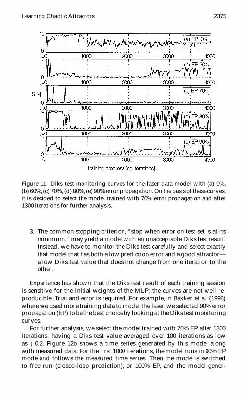1 Introduction

A time series measured from a deterministic chaotic system has the ap-pealing characteristic that its evolution is fully determined and yet its pre-dictability is limited due to exponential growth of errors in model or mea-surements A variety of data-driven analysis methods for this type of timeseries was collected in 1991 during the Santa Fe time-series competition(Weigend amp Gershenfeld 1994) The methods focused on either character-ization or prediction of the time series No attention was given to a thirdand much more appealing objective given the data and the assumptionthat it was produced by a deterministic chaotic system nd a set of modelequations that will produce a time series with identical chaotic character-istics having the same chaotic attractor The model could be based on rstprinciples if the system is well understood but here we assume knowl-edge of just the time series and use a neural networkndashbased black-boxmodel The choice for neural networks is inspired by the inherent stabilityof their iterated predictions as opposed to for example polynomial models(Aguirre amp Billings 1994) and local linear models (Farmer amp Sidorowich1987) Lapedes and Farber (1987) were among the rst who tried the neu-ral network approach In concise neural network jargon we formulate ourgoal train a network to learn the chaotic attractor A number of authorshave addressed this issue (Aguirre amp Billings 1994 Principe Rathie ampKuo 1992 Kuo amp Principe 1994 Deco amp Schurmann 1994 Rico-Martotilde nezKrischer Kevrekidis Kube amp Hudson 1992 Krischer et al 1993 AlbanoPassamente Hediger amp Farrell 1992) The common approach consists oftwo steps

1 Identify a model that makes accurate short-term predictions

2 Generate a long time series with the model by iterated prediction andcompare the nonlinear-dynamic characteristics of the generated timeseries with the original measured time series

Principe et al (1992) found that in many cases this approach fails themodel can make good short-term predictionsbut has not learned the chaoticattractor The method would be greatly improved if we could minimizedirectly the difference between the reconstructed attractors of the model-generated and measured data rather than minimizing prediction errorsHowever we cannot reconstruct the attractor without rst having a predic-tion model Therefore research is focused on how to optimize both steps

We highly reduce the chance of failure by integrating step 2 into step 1the model identication Rather than evaluating the model attractor aftertraining we monitor the attractor during training and introduce a new testdeveloped by Diks van Zwet Takens and de Goede (1996) as a stopping cri-terion It tests the null hypothesis that the reconstructed attractors of model-generated and measured data are the same The criterion directly measures





2 Data Sets









ddt

0

h

v

w

1

A D

0

v


vD

1

A (21)


3 Model Structure


ExnC1 D F(Exn) (31)



























with

Aij DmX

kD2


i1 (34)
















EzrnC1 D AEzr

n C EbynC1 (42)





or equivalently







ynC1 D CExn (46)



or
















Q DZ


2(Er ))2 (51)































7 Laser Data Model




























notation




yt D xt C mt (A3)







(A5)
















s2e D E[m2

t ] C E[2 2t C (btg)2 2 2






s2e D s2

m C s22

iexcl1 iexcl (bg)2t

1 iexcl (bg)2

cent |bg | 6D 1 (A13)


s2e D s2



iexcl1iexcl(bg)2t

1iexcl(bg)2

cent |bg | 6D 1 (A14)

and for large t

s2e D s2



iexcl1

1iexcl(gb)2

cent |gb | 6D 1 (A15)









s2e D s2


u )iexcl

1 iexcl b2t

1 iexcl b2

cent |b| 6D 1 (A16)



Acknowledgments


References




















































2 Data Sets









ddt

0

h

v

w

1

A D

0

v


vD

1

A (21)


3 Model Structure


ExnC1 D F(Exn) (31)



























with

Aij DmX

kD2


i1 (34)
















EzrnC1 D AEzr

n C EbynC1 (42)





or equivalently







ynC1 D CExn (46)



or
















Q DZ


2(Er ))2 (51)































7 Laser Data Model




























notation




yt D xt C mt (A3)







(A5)
















s2e D E[m2

t ] C E[2 2t C (btg)2 2 2






s2e D s2

m C s22

iexcl1 iexcl (bg)2t

1 iexcl (bg)2

cent |bg | 6D 1 (A13)


s2e D s2



iexcl1iexcl(bg)2t

1iexcl(bg)2

cent |bg | 6D 1 (A14)

and for large t

s2e D s2



iexcl1

1iexcl(gb)2

cent |gb | 6D 1 (A15)









s2e D s2


u )iexcl

1 iexcl b2t

1 iexcl b2

cent |b| 6D 1 (A16)



Acknowledgments


References























































ddt

0

h

v

w

1

A D

0

v


vD

1

A (21)


3 Model Structure


ExnC1 D F(Exn) (31)



























with

Aij DmX

kD2


i1 (34)
















EzrnC1 D AEzr

n C EbynC1 (42)





or equivalently







ynC1 D CExn (46)



or
















Q DZ


2(Er ))2 (51)































7 Laser Data Model




























notation




yt D xt C mt (A3)







(A5)
















s2e D E[m2

t ] C E[2 2t C (btg)2 2 2






s2e D s2

m C s22

iexcl1 iexcl (bg)2t

1 iexcl (bg)2

cent |bg | 6D 1 (A13)


s2e D s2



iexcl1iexcl(bg)2t

1iexcl(bg)2

cent |bg | 6D 1 (A14)

and for large t

s2e D s2



iexcl1

1iexcl(gb)2

cent |gb | 6D 1 (A15)









s2e D s2


u )iexcl

1 iexcl b2t

1 iexcl b2

cent |b| 6D 1 (A16)



Acknowledgments


References


















































ddt

0

h

v

w

1

A D

0

v


vD

1

A (21)


3 Model Structure


ExnC1 D F(Exn) (31)



























with

Aij DmX

kD2


i1 (34)
















EzrnC1 D AEzr

n C EbynC1 (42)





or equivalently







ynC1 D CExn (46)



or
















Q DZ


2(Er ))2 (51)































7 Laser Data Model




























notation




yt D xt C mt (A3)







(A5)
















s2e D E[m2

t ] C E[2 2t C (btg)2 2 2






s2e D s2

m C s22

iexcl1 iexcl (bg)2t

1 iexcl (bg)2

cent |bg | 6D 1 (A13)


s2e D s2



iexcl1iexcl(bg)2t

1iexcl(bg)2

cent |bg | 6D 1 (A14)

and for large t

s2e D s2



iexcl1

1iexcl(gb)2

cent |gb | 6D 1 (A15)









s2e D s2


u )iexcl

1 iexcl b2t

1 iexcl b2

cent |b| 6D 1 (A16)



Acknowledgments


References








































































with

Aij DmX

kD2


i1 (34)
















EzrnC1 D AEzr

n C EbynC1 (42)





or equivalently







ynC1 D CExn (46)



or
















Q DZ


2(Er ))2 (51)































7 Laser Data Model




























notation




yt D xt C mt (A3)







(A5)
















s2e D E[m2

t ] C E[2 2t C (btg)2 2 2






s2e D s2

m C s22

iexcl1 iexcl (bg)2t

1 iexcl (bg)2

cent |bg | 6D 1 (A13)


s2e D s2



iexcl1iexcl(bg)2t

1iexcl(bg)2

cent |bg | 6D 1 (A14)

and for large t

s2e D s2



iexcl1

1iexcl(gb)2

cent |gb | 6D 1 (A15)









s2e D s2


u )iexcl

1 iexcl b2t

1 iexcl b2

cent |b| 6D 1 (A16)



Acknowledgments


References
































































with

Aij DmX

kD2


i1 (34)
















EzrnC1 D AEzr

n C EbynC1 (42)





or equivalently







ynC1 D CExn (46)



or
















Q DZ


2(Er ))2 (51)































7 Laser Data Model




























notation




yt D xt C mt (A3)







(A5)
















s2e D E[m2

t ] C E[2 2t C (btg)2 2 2






s2e D s2

m C s22

iexcl1 iexcl (bg)2t

1 iexcl (bg)2

cent |bg | 6D 1 (A13)


s2e D s2



iexcl1iexcl(bg)2t

1iexcl(bg)2

cent |bg | 6D 1 (A14)

and for large t

s2e D s2



iexcl1

1iexcl(gb)2

cent |gb | 6D 1 (A15)









s2e D s2


u )iexcl

1 iexcl b2t

1 iexcl b2

cent |b| 6D 1 (A16)



Acknowledgments


References


























































with

Aij DmX

kD2


i1 (34)
















EzrnC1 D AEzr

n C EbynC1 (42)





or equivalently







ynC1 D CExn (46)



or
















Q DZ


2(Er ))2 (51)































7 Laser Data Model




























notation




yt D xt C mt (A3)







(A5)
















s2e D E[m2

t ] C E[2 2t C (btg)2 2 2






s2e D s2

m C s22

iexcl1 iexcl (bg)2t

1 iexcl (bg)2

cent |bg | 6D 1 (A13)


s2e D s2



iexcl1iexcl(bg)2t

1iexcl(bg)2

cent |bg | 6D 1 (A14)

and for large t

s2e D s2



iexcl1

1iexcl(gb)2

cent |gb | 6D 1 (A15)









s2e D s2


u )iexcl

1 iexcl b2t

1 iexcl b2

cent |b| 6D 1 (A16)



Acknowledgments


References






















































with

Aij DmX

kD2


i1 (34)
















EzrnC1 D AEzr

n C EbynC1 (42)





or equivalently







ynC1 D CExn (46)



or
















Q DZ


2(Er ))2 (51)































7 Laser Data Model




























notation




yt D xt C mt (A3)







(A5)
















s2e D E[m2

t ] C E[2 2t C (btg)2 2 2






s2e D s2

m C s22

iexcl1 iexcl (bg)2t

1 iexcl (bg)2

cent |bg | 6D 1 (A13)


s2e D s2



iexcl1iexcl(bg)2t

1iexcl(bg)2

cent |bg | 6D 1 (A14)

and for large t

s2e D s2



iexcl1

1iexcl(gb)2

cent |gb | 6D 1 (A15)









s2e D s2


u )iexcl

1 iexcl b2t

1 iexcl b2

cent |b| 6D 1 (A16)



Acknowledgments


References





























































EzrnC1 D AEzr

n C EbynC1 (42)





or equivalently







ynC1 D CExn (46)



or
















Q DZ


2(Er ))2 (51)































7 Laser Data Model




























notation




yt D xt C mt (A3)







(A5)
















s2e D E[m2

t ] C E[2 2t C (btg)2 2 2






s2e D s2

m C s22

iexcl1 iexcl (bg)2t

1 iexcl (bg)2

cent |bg | 6D 1 (A13)


s2e D s2



iexcl1iexcl(bg)2t

1iexcl(bg)2

cent |bg | 6D 1 (A14)

and for large t

s2e D s2



iexcl1

1iexcl(gb)2

cent |gb | 6D 1 (A15)









s2e D s2


u )iexcl

1 iexcl b2t

1 iexcl b2

cent |b| 6D 1 (A16)



Acknowledgments


References
























































EzrnC1 D AEzr

n C EbynC1 (42)





or equivalently







ynC1 D CExn (46)



or
















Q DZ


2(Er ))2 (51)































7 Laser Data Model




























notation




yt D xt C mt (A3)







(A5)
















s2e D E[m2

t ] C E[2 2t C (btg)2 2 2






s2e D s2

m C s22

iexcl1 iexcl (bg)2t

1 iexcl (bg)2

cent |bg | 6D 1 (A13)


s2e D s2



iexcl1iexcl(bg)2t

1iexcl(bg)2

cent |bg | 6D 1 (A14)

and for large t

s2e D s2



iexcl1

1iexcl(gb)2

cent |gb | 6D 1 (A15)









s2e D s2


u )iexcl

1 iexcl b2t

1 iexcl b2

cent |b| 6D 1 (A16)



Acknowledgments


References


















































EzrnC1 D AEzr

n C EbynC1 (42)





or equivalently







ynC1 D CExn (46)



or
















Q DZ


2(Er ))2 (51)































7 Laser Data Model




























notation




yt D xt C mt (A3)







(A5)
















s2e D E[m2

t ] C E[2 2t C (btg)2 2 2






s2e D s2

m C s22

iexcl1 iexcl (bg)2t

1 iexcl (bg)2

cent |bg | 6D 1 (A13)


s2e D s2



iexcl1iexcl(bg)2t

1iexcl(bg)2

cent |bg | 6D 1 (A14)

and for large t

s2e D s2



iexcl1

1iexcl(gb)2

cent |gb | 6D 1 (A15)









s2e D s2


u )iexcl

1 iexcl b2t

1 iexcl b2

cent |b| 6D 1 (A16)



Acknowledgments


References




















































ynC1 D CExn (46)



or
















Q DZ


2(Er ))2 (51)































7 Laser Data Model




























notation




yt D xt C mt (A3)







(A5)
















s2e D E[m2

t ] C E[2 2t C (btg)2 2 2






s2e D s2

m C s22

iexcl1 iexcl (bg)2t

1 iexcl (bg)2

cent |bg | 6D 1 (A13)


s2e D s2



iexcl1iexcl(bg)2t

1iexcl(bg)2

cent |bg | 6D 1 (A14)

and for large t

s2e D s2



iexcl1

1iexcl(gb)2

cent |gb | 6D 1 (A15)









s2e D s2


u )iexcl

1 iexcl b2t

1 iexcl b2

cent |b| 6D 1 (A16)



Acknowledgments


References



























































Q DZ


2(Er ))2 (51)































7 Laser Data Model




























notation




yt D xt C mt (A3)







(A5)
















s2e D E[m2

t ] C E[2 2t C (btg)2 2 2






s2e D s2

m C s22

iexcl1 iexcl (bg)2t

1 iexcl (bg)2

cent |bg | 6D 1 (A13)


s2e D s2



iexcl1iexcl(bg)2t

1iexcl(bg)2

cent |bg | 6D 1 (A14)

and for large t

s2e D s2



iexcl1

1iexcl(gb)2

cent |gb | 6D 1 (A15)









s2e D s2


u )iexcl

1 iexcl b2t

1 iexcl b2

cent |b| 6D 1 (A16)



Acknowledgments


References




















































Q DZ


2(Er ))2 (51)































7 Laser Data Model




























notation




yt D xt C mt (A3)







(A5)
















s2e D E[m2

t ] C E[2 2t C (btg)2 2 2






s2e D s2

m C s22

iexcl1 iexcl (bg)2t

1 iexcl (bg)2

cent |bg | 6D 1 (A13)


s2e D s2



iexcl1iexcl(bg)2t

1iexcl(bg)2

cent |bg | 6D 1 (A14)

and for large t

s2e D s2



iexcl1

1iexcl(gb)2

cent |gb | 6D 1 (A15)









s2e D s2


u )iexcl

1 iexcl b2t

1 iexcl b2

cent |b| 6D 1 (A16)



Acknowledgments


References








































































7 Laser Data Model




























notation




yt D xt C mt (A3)







(A5)
















s2e D E[m2

t ] C E[2 2t C (btg)2 2 2






s2e D s2

m C s22

iexcl1 iexcl (bg)2t

1 iexcl (bg)2

cent |bg | 6D 1 (A13)


s2e D s2



iexcl1iexcl(bg)2t

1iexcl(bg)2

cent |bg | 6D 1 (A14)

and for large t

s2e D s2



iexcl1

1iexcl(gb)2

cent |gb | 6D 1 (A15)









s2e D s2


u )iexcl

1 iexcl b2t

1 iexcl b2

cent |b| 6D 1 (A16)



Acknowledgments


References
































































7 Laser Data Model




























notation




yt D xt C mt (A3)







(A5)
















s2e D E[m2

t ] C E[2 2t C (btg)2 2 2






s2e D s2

m C s22

iexcl1 iexcl (bg)2t

1 iexcl (bg)2

cent |bg | 6D 1 (A13)


s2e D s2



iexcl1iexcl(bg)2t

1iexcl(bg)2

cent |bg | 6D 1 (A14)

and for large t

s2e D s2



iexcl1

1iexcl(gb)2

cent |gb | 6D 1 (A15)









s2e D s2


u )iexcl

1 iexcl b2t

1 iexcl b2

cent |b| 6D 1 (A16)



Acknowledgments


References





























































7 Laser Data Model




























notation




yt D xt C mt (A3)







(A5)
















s2e D E[m2

t ] C E[2 2t C (btg)2 2 2






s2e D s2

m C s22

iexcl1 iexcl (bg)2t

1 iexcl (bg)2

cent |bg | 6D 1 (A13)


s2e D s2



iexcl1iexcl(bg)2t

1iexcl(bg)2

cent |bg | 6D 1 (A14)

and for large t

s2e D s2



iexcl1

1iexcl(gb)2

cent |gb | 6D 1 (A15)









s2e D s2


u )iexcl

1 iexcl b2t

1 iexcl b2

cent |b| 6D 1 (A16)



Acknowledgments


References
























































7 Laser Data Model




























notation




yt D xt C mt (A3)







(A5)
















s2e D E[m2

t ] C E[2 2t C (btg)2 2 2






s2e D s2

m C s22

iexcl1 iexcl (bg)2t

1 iexcl (bg)2

cent |bg | 6D 1 (A13)


s2e D s2



iexcl1iexcl(bg)2t

1iexcl(bg)2

cent |bg | 6D 1 (A14)

and for large t

s2e D s2



iexcl1

1iexcl(gb)2

cent |gb | 6D 1 (A15)









s2e D s2


u )iexcl

1 iexcl b2t

1 iexcl b2

cent |b| 6D 1 (A16)



Acknowledgments


References


















































7 Laser Data Model




























notation




yt D xt C mt (A3)







(A5)
















s2e D E[m2

t ] C E[2 2t C (btg)2 2 2






s2e D s2

m C s22

iexcl1 iexcl (bg)2t

1 iexcl (bg)2

cent |bg | 6D 1 (A13)


s2e D s2



iexcl1iexcl(bg)2t

1iexcl(bg)2

cent |bg | 6D 1 (A14)

and for large t

s2e D s2



iexcl1

1iexcl(gb)2

cent |gb | 6D 1 (A15)









s2e D s2


u )iexcl

1 iexcl b2t

1 iexcl b2

cent |b| 6D 1 (A16)



Acknowledgments


References








































































notation




yt D xt C mt (A3)







(A5)
















s2e D E[m2

t ] C E[2 2t C (btg)2 2 2






s2e D s2

m C s22

iexcl1 iexcl (bg)2t

1 iexcl (bg)2

cent |bg | 6D 1 (A13)


s2e D s2



iexcl1iexcl(bg)2t

1iexcl(bg)2

cent |bg | 6D 1 (A14)

and for large t

s2e D s2



iexcl1

1iexcl(gb)2

cent |gb | 6D 1 (A15)









s2e D s2


u )iexcl

1 iexcl b2t

1 iexcl b2

cent |b| 6D 1 (A16)



Acknowledgments


References



































































notation




yt D xt C mt (A3)







(A5)
















s2e D E[m2

t ] C E[2 2t C (btg)2 2 2






s2e D s2

m C s22

iexcl1 iexcl (bg)2t

1 iexcl (bg)2

cent |bg | 6D 1 (A13)


s2e D s2



iexcl1iexcl(bg)2t

1iexcl(bg)2

cent |bg | 6D 1 (A14)

and for large t

s2e D s2



iexcl1

1iexcl(gb)2

cent |gb | 6D 1 (A15)









s2e D s2


u )iexcl

1 iexcl b2t

1 iexcl b2

cent |b| 6D 1 (A16)



Acknowledgments


References































































notation




yt D xt C mt (A3)







(A5)
















s2e D E[m2

t ] C E[2 2t C (btg)2 2 2






s2e D s2

m C s22

iexcl1 iexcl (bg)2t

1 iexcl (bg)2

cent |bg | 6D 1 (A13)


s2e D s2



iexcl1iexcl(bg)2t

1iexcl(bg)2

cent |bg | 6D 1 (A14)

and for large t

s2e D s2



iexcl1

1iexcl(gb)2

cent |gb | 6D 1 (A15)









s2e D s2


u )iexcl

1 iexcl b2t

1 iexcl b2

cent |b| 6D 1 (A16)



Acknowledgments


References

























































notation




yt D xt C mt (A3)







(A5)
















s2e D E[m2

t ] C E[2 2t C (btg)2 2 2






s2e D s2

m C s22

iexcl1 iexcl (bg)2t

1 iexcl (bg)2

cent |bg | 6D 1 (A13)


s2e D s2



iexcl1iexcl(bg)2t

1iexcl(bg)2

cent |bg | 6D 1 (A14)

and for large t

s2e D s2



iexcl1

1iexcl(gb)2

cent |gb | 6D 1 (A15)









s2e D s2


u )iexcl

1 iexcl b2t

1 iexcl b2

cent |b| 6D 1 (A16)



Acknowledgments


References

















































notation




yt D xt C mt (A3)







(A5)
















s2e D E[m2

t ] C E[2 2t C (btg)2 2 2






s2e D s2

m C s22

iexcl1 iexcl (bg)2t

1 iexcl (bg)2

cent |bg | 6D 1 (A13)


s2e D s2



iexcl1iexcl(bg)2t

1iexcl(bg)2

cent |bg | 6D 1 (A14)

and for large t

s2e D s2



iexcl1

1iexcl(gb)2

cent |gb | 6D 1 (A15)









s2e D s2


u )iexcl

1 iexcl b2t

1 iexcl b2

cent |b| 6D 1 (A16)



Acknowledgments


References


















































s2e D E[m2

t ] C E[2 2t C (btg)2 2 2






s2e D s2

m C s22

iexcl1 iexcl (bg)2t

1 iexcl (bg)2

cent |bg | 6D 1 (A13)


s2e D s2



iexcl1iexcl(bg)2t

1iexcl(bg)2

cent |bg | 6D 1 (A14)

and for large t

s2e D s2



iexcl1

1iexcl(gb)2

cent |gb | 6D 1 (A15)









s2e D s2


u )iexcl

1 iexcl b2t

1 iexcl b2

cent |b| 6D 1 (A16)



Acknowledgments


References




















































s2e D s2


u )iexcl

1 iexcl b2t

1 iexcl b2

cent |b| 6D 1 (A16)



Acknowledgments


References









































































































Documents

Learning Chaotic Attractors by Neural Networks Chaotic Attractors by Neural Networks Rembrandt Bakker DelftChemTech, Delft University of Technology, 2628 BL Delft, The Netherlands