Embed Size (px)
Citation preview
Lattice theory and Toeplitz determinants
Albrecht Bottcher, Lenny Fukshansky,Stephan Ramon Garcia, and Hiren Maharaj
Abstract. This is a survey of our recent joint investigations of lattices that aregenerated by finite Abelian groups. In the case of cyclic groups, the volume ofa fundamental domain of such a lattice is a perturbed Toeplitz determinantwith a simple Fisher-Hartwig symbol. For general groups, the situation ismore complicated, but it can still be tackled by pure matrix theory. Our mainresult on the lattices under consideration states that they always have a basisof minimal vectors, while our results in the other direction concern exact andasymptotic formulas for perturbed Toeplitz determinants. The survey is aslightly modified version of the talk given by the first author at the HumboldtKolleg and the IWOTA in Tbilisi in 2015. It is mainly for operator theoristsand therefore also contains an introduction to the basics of lattice theory.
MSC 2010. Primary 11H31. Secondary 15A15, 15B05, 47B35, 52C17
Keywords. Lattice packing, finite Abelian group, perturbed Toeplitz determi-nant, Fisher-Hartwig symbol
1. Introduction
The determinant of the n× n analogue An of the matrix
A6 =
6 −4 1 0 0 1−4 6 −4 1 0 0
1 −4 6 −4 1 00 1 −4 6 −4 10 0 1 −4 6 −41 0 0 1 −4 6
Fukshansky acknowledges support by Simons Foundation grant #279155 and by NSA grant#130907, Garcia acknowledges support by NSF grant DMS-1265973.
2 Bottcher, Fukshansky, Garcia, and Maharaj
is detAn = (n + 1)3 ∼ n3, whereas the determinant of the n × n analogue Tn ofthe matrix
T6 =
6 −4 1 0 0 0−4 6 −4 1 0 0
1 −4 6 −4 1 00 1 −4 6 −4 10 0 1 −4 6 −40 0 0 1 −4 6
equals
detTn =(n+ 1)(n+ 2)2(n+ 3)
12∼ n4
12.
(The notation an ∼ bn means that an/bn → 1.) The determinants detAn emergein a problem of lattice theory [6] and the formula detAn = (n+1)3 was establishedonly in [6], while the determinants detTn are special cases of the well-known Fisher-Hartwig determinants one encounters in statistical physics [11, 12]. The matricesTn are principal truncations of an infinite Toeplitz matrix. This is not true of thematrices An, but these are simple corner perturbations of Tn.
The observations made above motivated us to undertake studies into twodirections. First, the ability to compute the determinants of An, which arise whenconsidering lattices associated to cyclic groups, encouraged us to turn to latticesthat are generated by arbitrary finite Abelian groups. And secondly, intrigued bythe question why the corner perturbations lower the growth of the determinantsfrom n4 to n3, we explored the determinants of perturbed Toeplitz matrices withmore general Fisher-Hartwig symbols.
Our investigations resulted in the two papers [5, 6], and here we want togive a survey of these papers. This survey is intended for operator theorists. Weare therefore concise when dealing with Toeplitz operators and matrices, but weconsider it as useful to devote due space to some basics of lattice theory. Sections 1to 6 are dedicated to lattice theory, and in the remaining Sections 7 to 9 we embarkon Toeplitz determinants.
2. Examples of lattices
By an n-dimensional lattice we mean a discrete subgroup L of the Euclidean spaceRn. The lattice is said to have full rank if
spanRL = Rn,
where spanRL is the intersection of all linear subspaces of Rn which contain L.Unless otherwise stated, all lattices considered in this paper are of full rank andhence we omit the attribute “full-rank”. Of course, Zn is the simplest example ofan n-dimensional lattice.
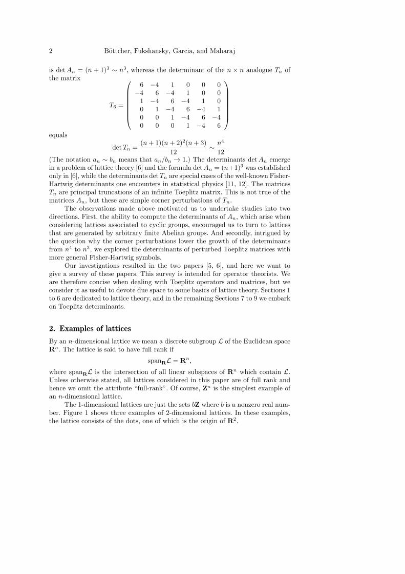
The 1-dimensional lattices are just the sets bZ where b is a nonzero real num-ber. Figure 1 shows three examples of 2-dimensional lattices. In these examples,the lattice consists of the dots, one of which is the origin of R2.
Lattice theory and Toeplitz determinants 3
Figure 1. Three 2-dimensional lattices.
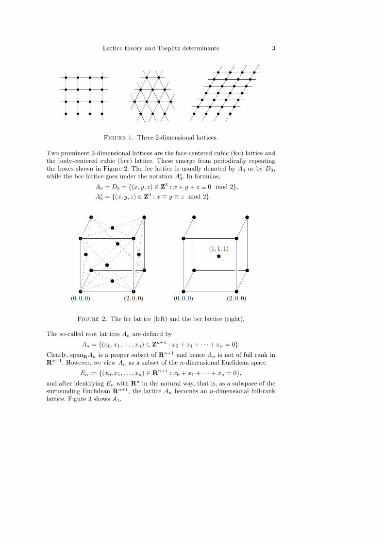
Two prominent 3-dimensional lattices are the face-centered cubic (fcc) lattice andthe body-centered cubic (bcc) lattice. These emerge from periodically repeatingthe boxes shown in Figure 2. The fcc lattice is usually denoted by A3 or by D3,while the bcc lattice goes under the notation A∗3. In formulas,
A3 = D3 = {(x, y, z) ∈ Z3 : x+ y + z ≡ 0 mod 2},A∗3 = {(x, y, z) ∈ Z3 : x ≡ y ≡ z mod 2}.
Figure 2. The fcc lattice (left) and the bcc lattice (right).
The so-called root lattices An are defined by
An = {(x0, x1, . . . , xn) ∈ Zn+1 : x0 + x1 + · · ·+ xn = 0}.Clearly, spanRAn is a proper subset of Rn+1 and hence An is not of full rank inRn+1. However, we view An as a subset of the n-dimensional Euclidean space
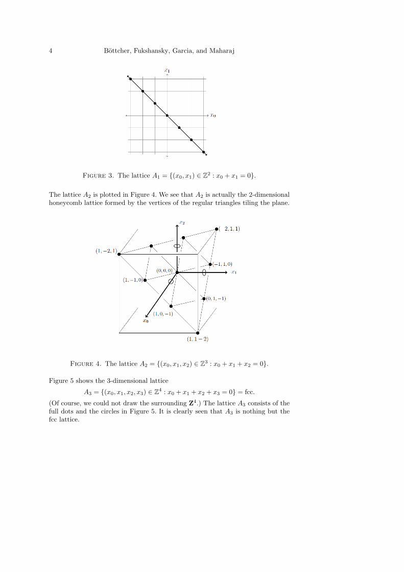
En := {(x0, x1, . . . , xn) ∈ Rn+1 : x0 + x1 + · · ·+ xn = 0},and after identifying En with Rn in the natural way, that is, as a subspace of thesurrounding Euclidean Rn+1, the lattice An becomes an n-dimensional full-ranklattice. Figure 3 shows A1.
4 Bottcher, Fukshansky, Garcia, and Maharaj
Figure 3. The lattice A1 = {(x0, x1) ∈ Z2 : x0 + x1 = 0}.
The lattice A2 is plotted in Figure 4. We see that A2 is actually the 2-dimensionalhoneycomb lattice formed by the vertices of the regular triangles tiling the plane.
Figure 4. The lattice A2 = {(x0, x1, x2) ∈ Z3 : x0 + x1 + x2 = 0}.
Figure 5 shows the 3-dimensional lattice
A3 = {(x0, x1, x2, x3) ∈ Z4 : x0 + x1 + x2 + x3 = 0} = fcc.
(Of course, we could not draw the surrounding Z4.) The lattice A3 consists of thefull dots and the circles in Figure 5. It is clearly seen that A3 is nothing but thefcc lattice.
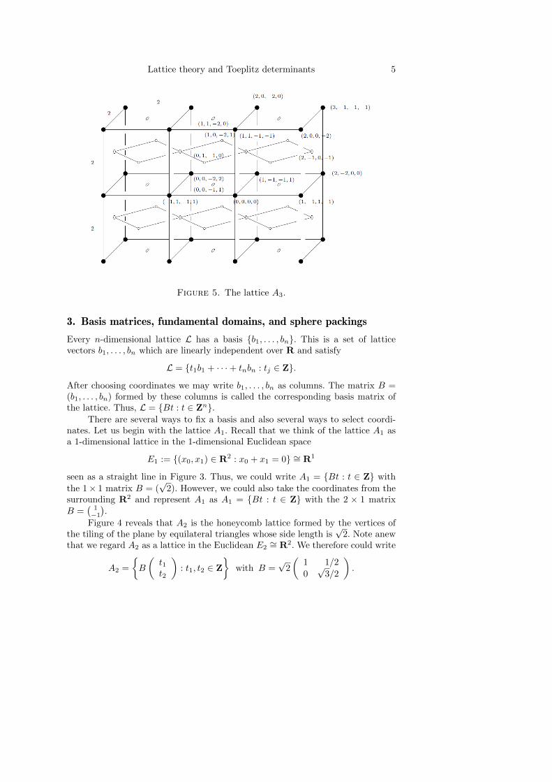
Lattice theory and Toeplitz determinants 5
Figure 5. The lattice A3.
3. Basis matrices, fundamental domains, and sphere packings
Every n-dimensional lattice L has a basis {b1, . . . , bn}. This is a set of latticevectors b1, . . . , bn which are linearly independent over R and satisfy
L = {t1b1 + · · ·+ tnbn : tj ∈ Z}.
After choosing coordinates we may write b1, . . . , bn as columns. The matrix B =(b1, . . . , bn) formed by these columns is called the corresponding basis matrix ofthe lattice. Thus, L = {Bt : t ∈ Zn}.
There are several ways to fix a basis and also several ways to select coordi-nates. Let us begin with the lattice A1. Recall that we think of the lattice A1 asa 1-dimensional lattice in the 1-dimensional Euclidean space
E1 := {(x0, x1) ∈ R2 : x0 + x1 = 0} ∼= R1
seen as a straight line in Figure 3. Thus, we could write A1 = {Bt : t ∈ Z} with
the 1× 1 matrix B = (√
2). However, we could also take the coordinates from thesurrounding R2 and represent A1 as A1 = {Bt : t ∈ Z} with the 2 × 1 matrixB =
(1−1).
Figure 4 reveals that A2 is the honeycomb lattice formed by the vertices ofthe tiling of the plane by equilateral triangles whose side length is
√2. Note anew
that we regard A2 as a lattice in the Euclidean E2∼= R2. We therefore could write
A2 =
{B
(t1t2
): t1, t2 ∈ Z
}with B =
√2
(1 1/2
0√
3/2
).
6 Bottcher, Fukshansky, Garcia, and Maharaj
Again we prefer taking the coordinates from the surrounding R2. This gives thealternative representation
A2 =
{B
(t1t2
): t1, t2 ∈ Z
}with B =
1 00 1−1 −1
.
We know that A3 is the fcc lattice. The side length of the cubes is 2.The centers of the lower, left, and front faces of the upper-right cube in Fig-ure 5 form a basis for A3. In R3, these centers could be given the coordinates(1, 1, 0), (0, 1, 1), (1, 0, 1), resulting in the representation
A3 =
B t1
t2t3
: tj ∈ Z
with B =
1 0 11 1 00 1 1
.
Figure 5 shows that in the surrounding R4 the coordinates of these centers are(1,−1, 0, 0), (1, 0,−1, 0), (1, 0, 0,−1). This leads to the description
A3 =
B t1
t2t3
: tj ∈ Z
with B =
1 1 1−1 0 0
0 −1 00 0 −1
.
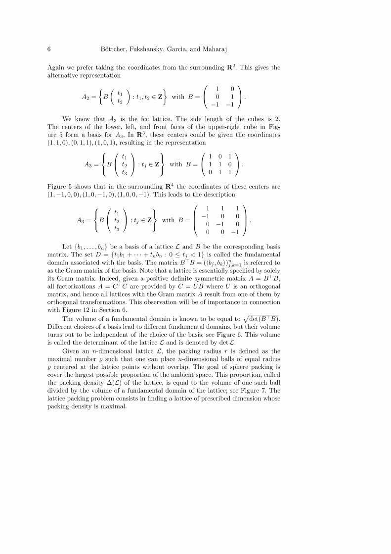
Let {b1, . . . , bn} be a basis of a lattice L and B be the corresponding basismatrix. The set D = {t1b1 + · · · + tnbn : 0 ≤ tj < 1} is called the fundamentaldomain associated with the basis. The matrix B>B = (〈bj , bk〉)nj,k=1 is referred toas the Gram matrix of the basis. Note that a lattice is essentially specified by solelyits Gram matrix. Indeed, given a positive definite symmetric matrix A = B>B,all factorizations A = C>C are provided by C = UB where U is an orthogonalmatrix, and hence all lattices with the Gram matrix A result from one of them byorthogonal transformations. This observation will be of importance in connectionwith Figure 12 in Section 6.
The volume of a fundamental domain is known to be equal to√
det(B>B).Different choices of a basis lead to different fundamental domains, but their volumeturns out to be independent of the choice of the basis; see Figure 6. This volumeis called the determinant of the lattice L and is denoted by detL.
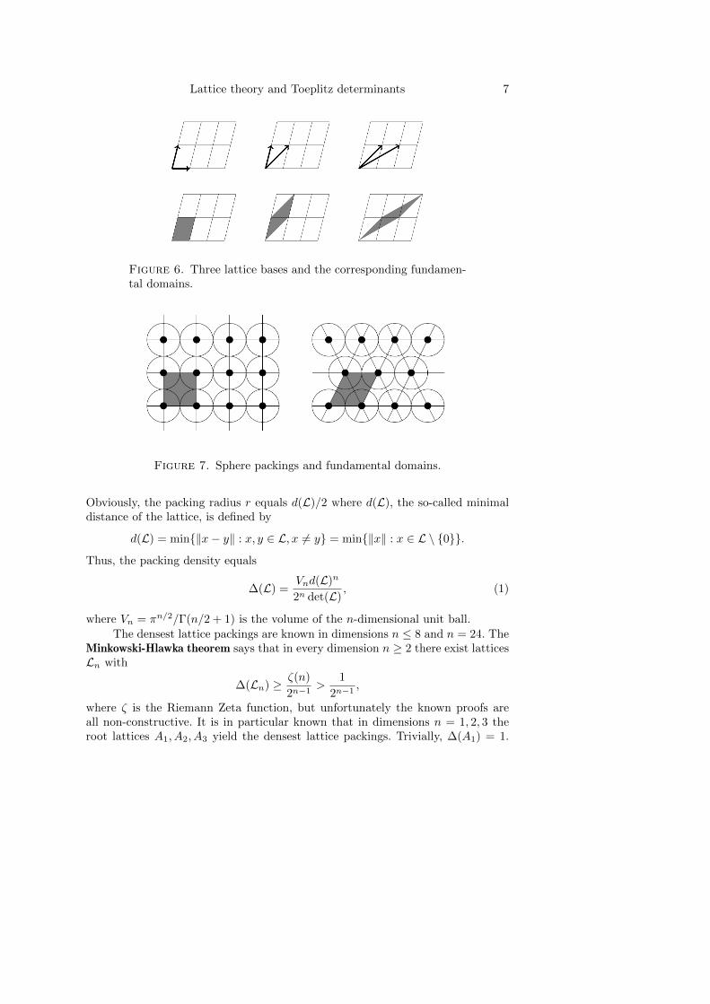
Given an n-dimensional lattice L, the packing radius r is defined as themaximal number % such that one can place n-dimensional balls of equal radius% centered at the lattice points without overlap. The goal of sphere packing iscover the largest possible proportion of the ambient space. This proportion, calledthe packing density ∆(L) of the lattice, is equal to the volume of one such balldivided by the volume of a fundamental domain of the lattice; see Figure 7. Thelattice packing problem consists in finding a lattice of prescribed dimension whosepacking density is maximal.
Lattice theory and Toeplitz determinants 7
Figure 6. Three lattice bases and the corresponding fundamen-tal domains.
Figure 7. Sphere packings and fundamental domains.
Obviously, the packing radius r equals d(L)/2 where d(L), the so-called minimaldistance of the lattice, is defined by
d(L) = min{‖x− y‖ : x, y ∈ L, x 6= y} = min{‖x‖ : x ∈ L \ {0}}.
Thus, the packing density equals
∆(L) =Vnd(L)n
2n det(L), (1)
where Vn = πn/2/Γ(n/2 + 1) is the volume of the n-dimensional unit ball.
The densest lattice packings are known in dimensions n ≤ 8 and n = 24. TheMinkowski-Hlawka theorem says that in every dimension n ≥ 2 there exist latticesLn with
∆(Ln) ≥ ζ(n)
2n−1>
1
2n−1,
where ζ is the Riemann Zeta function, but unfortunately the known proofs areall non-constructive. It is in particular known that in dimensions n = 1, 2, 3 theroot lattices A1, A2, A3 yield the densest lattice packings. Trivially, ∆(A1) = 1.
8 Bottcher, Fukshansky, Garcia, and Maharaj
For n = 2, 3, the densities and the Minkowski-Hlawka bounds are
∆(A2) =π√12≈ 0.9069, ζ(2)/2 ≈ 0.8224,
∆(A3) = ∆(fcc) = ∆(D3) =π√18≈ 0.7404, ζ(3)/22 ≈ 0.3005.
For 4 ≤ n ≤ 8, the lattices delivering the densest lattice packings are D4, D5, E6,E7, E8 with
D4 = {(x1, x2, x3, x4) ∈ Z4 : x1 + x2 + x3 + x4 ≡ 0 mod 2},D5 = {(x1, x2, x3, x4, x5) ∈ Z5 : x1 + x2 + x3 + x4 + x5 ≡ 0 mod 2},
E8 = {(x1, . . . , x8) ∈ Z8 : all xi ∈ Z or all xi ∈ Z +1
2,
x1 + · · ·+ x8 ≡ 0 mod 2},E7 = {(x1, . . . , x8) ∈ E8 : x1 + · · ·+ x8 = 0},E6 = {(x1, . . . , x8) ∈ E8 : x6 = x7 = x8},
and in dimension n = 24 the champion is the Leech lattice Λ24 with
∆(Λ24) =π12
479 001 600≈ 0.001 930.
(Note that ∆(Λ24) is about 10 000 times better than the Minkowksi-Hlawka boundζ(24)/223 ≈ 0.000 000 119.) We refer to Conway and Sloane’s book [10] for moreon this topic.
4. Lattices from finite Abelian groups
In many dimensions below around 1 000, lattices with a packing density greaterthan the Minkowski-Hlawka bound are known. However, for general dimensions n,so far no one has found lattices whose packing density reaches the Minkowski-Hlawka bound. The best known lattices come from algebraic constructions. Weconfine ourselves to referring to the books [17, 18]. One such construction useselliptic curves. An elliptic curve over R is defined by
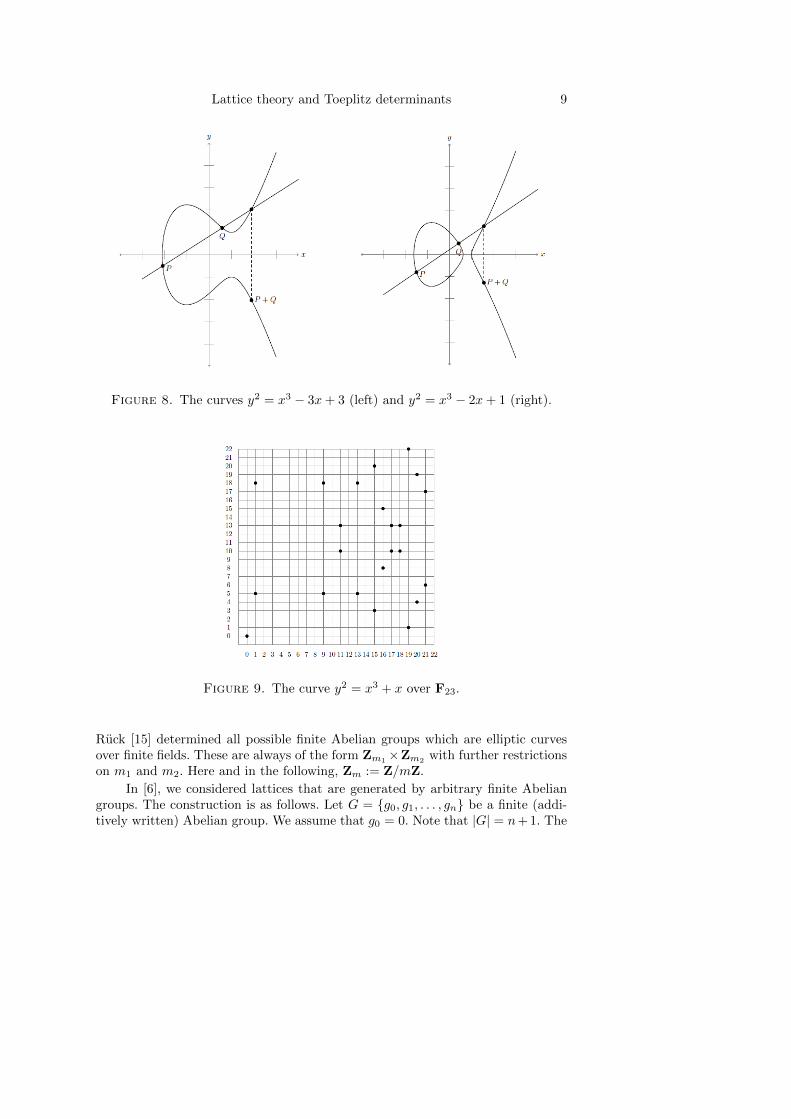
E = {(x, y) ∈ R2 : y2 = x3 + ax+ b},where a, b ∈ R satisfy 4a3 + 27b2 6= 0. Such a curve, together with a point atinfinity, is an Abelian group. Everyone has already seen pictures like those inFigure 8, which show the group operation in E.
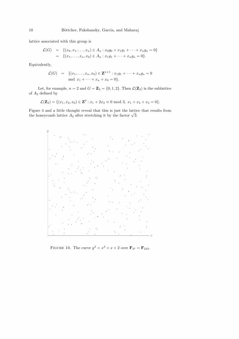
An elliptic curve over a finite field Fq, where q = pm is a prime power, is theset
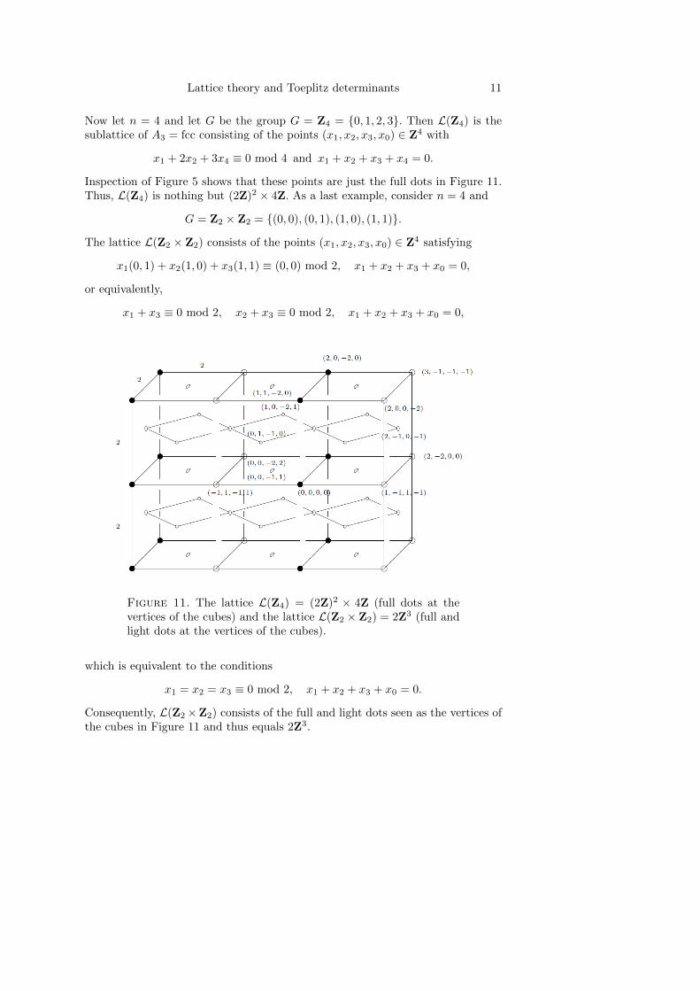
E = {(x, y) ∈ Fq : y2 = x3 + ax+ b}.Here a, b ∈ Fq and 4a3 + 27b2 6= 0. Such a curve, together with a point at infinity,is a finite Abelian group. The group operation can be given by translating thegeometric construction in Figure 8 into algebraic formulas. Figures 9 and 10 showtwo examples.
Lattice theory and Toeplitz determinants 9
Figure 8. The curves y2 = x3 − 3x+ 3 (left) and y2 = x3 − 2x+ 1 (right).
Figure 9. The curve y2 = x3 + x over F23.
Ruck [15] determined all possible finite Abelian groups which are elliptic curvesover finite fields. These are always of the form Zm1×Zm2 with further restrictionson m1 and m2. Here and in the following, Zm := Z/mZ.
In [6], we considered lattices that are generated by arbitrary finite Abeliangroups. The construction is as follows. Let G = {g0, g1, . . . , gn} be a finite (addi-tively written) Abelian group. We assume that g0 = 0. Note that |G| = n+ 1. The
10 Bottcher, Fukshansky, Garcia, and Maharaj
lattice associated with this group is
L(G) = {(x0, x1, . . . , xn) ∈ An : x0g0 + x1g1 + · · ·+ xngn = 0}= {(x1, . . . , xn, x0) ∈ An : x1g1 + · · ·+ xngn = 0}.
Equivalently,
L(G) = {(x1, . . . , xn, x0) ∈ Zn+1 : x1g1 + · · ·+ xngn = 0
and x1 + · · ·+ xn + x0 = 0}.
Let, for example, n = 2 and G = Z3 = {0, 1, 2}. Then L(Z3) is the sublatticeof A2 defined by
L(Z3) = {(x1, x2, x0) ∈ Z3 : x1 + 2x2 ≡ 0 mod 3, x1 + x2 + x3 = 0}.
Figure 4 and a little thought reveal that this is just the lattice that results fromthe honeycomb lattice A2 after stretching it by the factor
√3.
Figure 10. The curve y2 = x3 + x+ 2 over F35 = F243.
Lattice theory and Toeplitz determinants 11
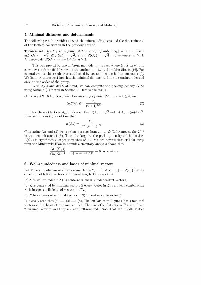
Now let n = 4 and let G be the group G = Z4 = {0, 1, 2, 3}. Then L(Z4) is thesublattice of A3 = fcc consisting of the points (x1, x2, x3, x0) ∈ Z4 with
x1 + 2x2 + 3x4 ≡ 0 mod 4 and x1 + x2 + x3 + x4 = 0.
Inspection of Figure 5 shows that these points are just the full dots in Figure 11.Thus, L(Z4) is nothing but (2Z)2 × 4Z. As a last example, consider n = 4 and
G = Z2 × Z2 = {(0, 0), (0, 1), (1, 0), (1, 1)}.
The lattice L(Z2 × Z2) consists of the points (x1, x2, x3, x0) ∈ Z4 satisfying
x1(0, 1) + x2(1, 0) + x3(1, 1) ≡ (0, 0) mod 2, x1 + x2 + x3 + x0 = 0,
or equivalently,
x1 + x3 ≡ 0 mod 2, x2 + x3 ≡ 0 mod 2, x1 + x2 + x3 + x0 = 0,
Figure 11. The lattice L(Z4) = (2Z)2 × 4Z (full dots at thevertices of the cubes) and the lattice L(Z2 × Z2) = 2Z3 (full andlight dots at the vertices of the cubes).
which is equivalent to the conditions
x1 = x2 = x3 ≡ 0 mod 2, x1 + x2 + x3 + x0 = 0.
Consequently, L(Z2×Z2) consists of the full and light dots seen as the vertices ofthe cubes in Figure 11 and thus equals 2Z3.
12 Bottcher, Fukshansky, Garcia, and Maharaj
5. Minimal distances and determinants
The following result provides us with the minimal distances and the determinantsof the lattices considered in the previous section.
Theorem 5.1. Let Gn be a finite Abelian group of order |Gn| = n + 1. Then
d(L(G2)) =√
8, d(L(G3)) =√
6, and d(L(Gn)) =√
4 = 2 whenever n ≥ 4.Moreover, detL(Gn) = (n+ 1)3 for n ≥ 2.
This was proved by two different methods in the case where Gn is an ellipticcurve over a finite field by two of the authors in [13] and by Min Sha in [16]. Forgeneral groups this result was established by yet another method in our paper [6].We find it rather surprising that the minimal distance and the determinant dependonly on the order of the group.
With d(L) and detL at hand, we can compute the packing density ∆(L)using formula (1) stated in Section 3. Here is the result.
Corollary 5.2. If Gn is a finite Abelian group of order |Gn| = n+ 1 ≥ 4, then
∆(L(Gn)) =Vn
(n+ 1)3/2. (2)
For the root lattices An, it is known that d(An) =√
2 and detAn = (n+1)1/2.Inserting this in (1) we obtain that
∆(An) =Vn
2n/2(n+ 1)1/2. (3)
Comparing (2) and (3) we see that passage from An to L(Gn) removed the 2n/2
in the denominator of (3), Thus, for large n, the packing density of the latticesL(Gn) is significantly larger than that of An. We are nevertheless still far awayfrom the Minkowski-Hlawka bound: elementary analysis shows that
∆(L(Gn))
ζ(n)/2n−1=
1
2n2 log2 n−n+O(1)
→ 0 as n→∞.
6. Well-roundedness and bases of minimal vectors
Let L be an n-dimensional lattice and let S(L) = {x ∈ L : ‖x‖ = d(L)} be thecollection of lattice vectors of minimal length. One says that
(a) L is well-rounded if S(L) contains n linearly independent vectors,
(b) L is generated by minimal vectors if every vector in L is a linear combinationwith integer coefficients of vectors in S(L),
(c) L has a basis of minimal vectors if S(L) contains a basis for L.
It is easily seen that (c) =⇒ (b) =⇒ (a). The left lattice in Figure 1 has 4 minimalvectors and a basis of minimal vectors. The two other lattices in Figure 1 have2 minimal vectors and they are not well-rounded. (Note that the middle lattice
Lattice theory and Toeplitz determinants 13
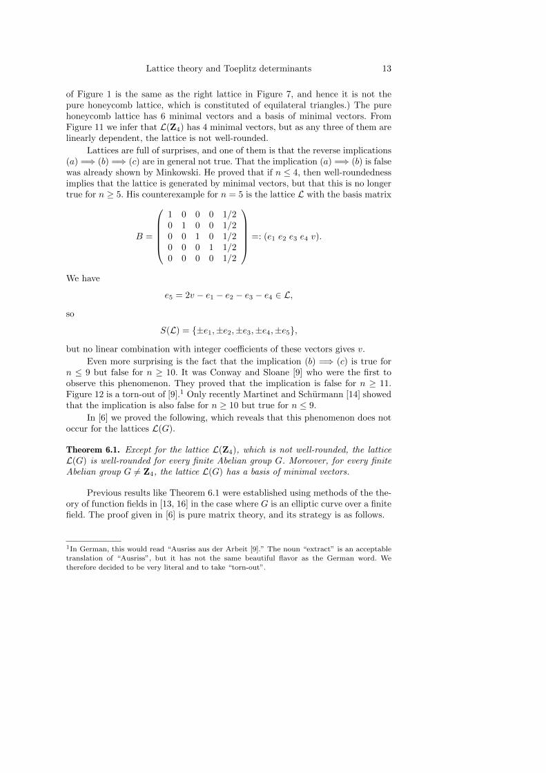
of Figure 1 is the same as the right lattice in Figure 7, and hence it is not thepure honeycomb lattice, which is constituted of equilateral triangles.) The purehoneycomb lattice has 6 minimal vectors and a basis of minimal vectors. FromFigure 11 we infer that L(Z4) has 4 minimal vectors, but as any three of them arelinearly dependent, the lattice is not well-rounded.
Lattices are full of surprises, and one of them is that the reverse implications(a) =⇒ (b) =⇒ (c) are in general not true. That the implication (a) =⇒ (b) is falsewas already shown by Minkowski. He proved that if n ≤ 4, then well-roundednessimplies that the lattice is generated by minimal vectors, but that this is no longertrue for n ≥ 5. His counterexample for n = 5 is the lattice L with the basis matrix
B =
1 0 0 0 1/20 1 0 0 1/20 0 1 0 1/20 0 0 1 1/20 0 0 0 1/2
=: (e1 e2 e3 e4 v).
We have
e5 = 2v − e1 − e2 − e3 − e4 ∈ L,
so
S(L) = {±e1,±e2,±e3,±e4,±e5},
but no linear combination with integer coefficients of these vectors gives v.
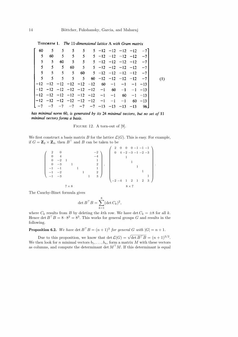
Even more surprising is the fact that the implication (b) =⇒ (c) is true forn ≤ 9 but false for n ≥ 10. It was Conway and Sloane [9] who were the first toobserve this phenomenon. They proved that the implication is false for n ≥ 11.Figure 12 is a torn-out of [9].1 Only recently Martinet and Schurmann [14] showedthat the implication is also false for n ≥ 10 but true for n ≤ 9.
In [6] we proved the following, which reveals that this phenomenon does notoccur for the lattices L(G).
Theorem 6.1. Except for the lattice L(Z4), which is not well-rounded, the latticeL(G) is well-rounded for every finite Abelian group G. Moreover, for every finiteAbelian group G 6= Z4, the lattice L(G) has a basis of minimal vectors.
Previous results like Theorem 6.1 were established using methods of the the-ory of function fields in [13, 16] in the case where G is an elliptic curve over a finitefield. The proof given in [6] is pure matrix theory, and its strategy is as follows.
1In German, this would read “Ausriss aus der Arbeit [9].” The noun “extract” is an acceptable
translation of “Ausriss”, but it has not the same beautiful flavor as the German word. Wetherefore decided to be very literal and to take “torn-out”.
14 Bottcher, Fukshansky, Garcia, and Maharaj
Figure 12. A torn-out of [9].
We first construct a basis matrix B for the lattice L(G). This is easy. For example,if G = Z2 × Z4, then B> and B can be taken to be
2 0 −2
0 4 −40 −2 1 1
0 −3 1 2
−1 −1 1 1−1 −2 1 2
−1 −3 1 3
,
2 0 0 0 −1 −1 −1
0 4 −2 −3 −1 −2 −3
1
1
1
1
1
−2 −4 1 2 1 2 3
.
7× 8 8× 7
The Cauchy-Binet formula gives
detB>B =
8∑k=1
(detCk)2,
where Ck results from B by deleting the kth row. We have detCk = ±8 for all k.Hence detB>B = 8 · 82 = 83. This works for general groups G and results in thefollowing.
Proposition 6.2. We have detB>B = (n+ 1)3 for general G with |G| = n+ 1.
Due to this proposition, we know that detL(G) =√
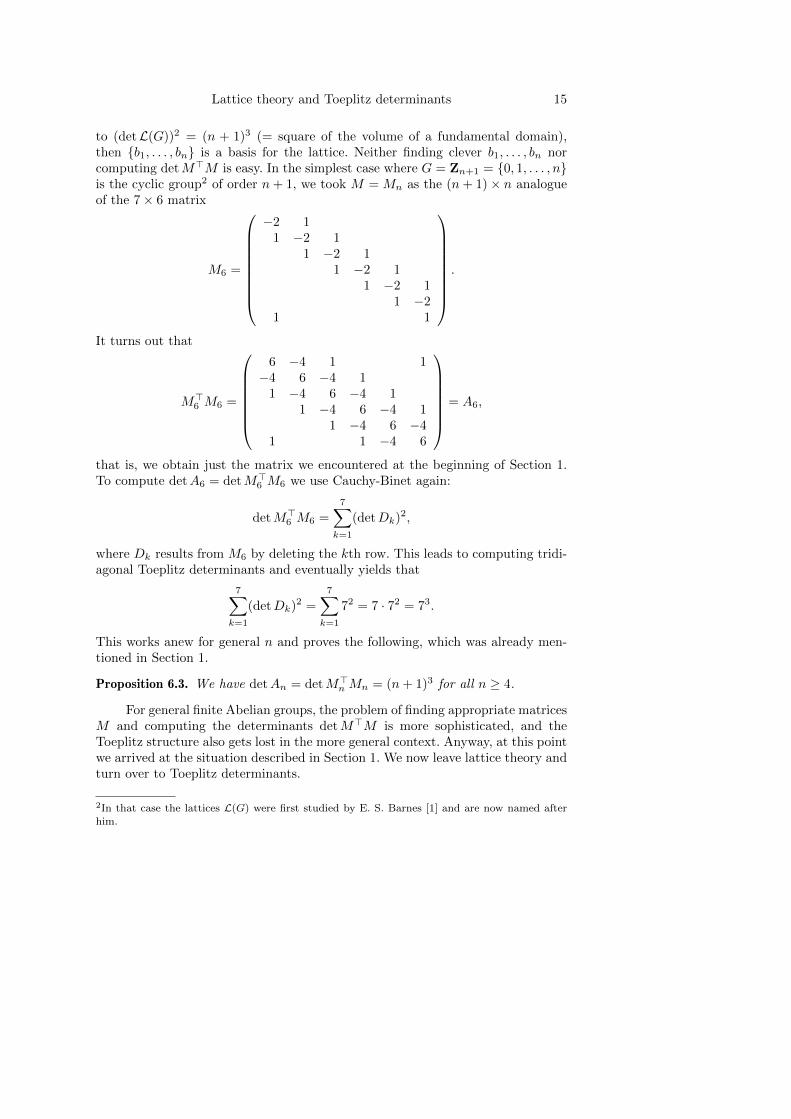
detB>B = (n + 1)3/2.We then look for n minimal vectors b1, . . . , bn, form a matrix M with these vectorsas columns, and compute the determinant detM>M . If this determinant is equal
Lattice theory and Toeplitz determinants 15
to (detL(G))2 = (n + 1)3 (= square of the volume of a fundamental domain),then {b1, . . . , bn} is a basis for the lattice. Neither finding clever b1, . . . , bn norcomputing detM>M is easy. In the simplest case where G = Zn+1 = {0, 1, . . . , n}is the cyclic group2 of order n+ 1, we took M = Mn as the (n+ 1)× n analogueof the 7× 6 matrix
M6 =
−2 11 −2 1
1 −2 11 −2 1
1 −2 11 −2
1 1
.
It turns out that
M>6 M6 =
6 −4 1 1−4 6 −4 1
1 −4 6 −4 11 −4 6 −4 1
1 −4 6 −41 1 −4 6
= A6,
that is, we obtain just the matrix we encountered at the beginning of Section 1.To compute detA6 = detM>6 M6 we use Cauchy-Binet again:
detM>6 M6 =
7∑k=1
(detDk)2,
where Dk results from M6 by deleting the kth row. This leads to computing tridi-agonal Toeplitz determinants and eventually yields that
7∑k=1
(detDk)2 =
7∑k=1
72 = 7 · 72 = 73.
This works anew for general n and proves the following, which was already men-tioned in Section 1.
Proposition 6.3. We have detAn = detM>nMn = (n+ 1)3 for all n ≥ 4.
For general finite Abelian groups, the problem of finding appropriate matricesM and computing the determinants detM>M is more sophisticated, and theToeplitz structure also gets lost in the more general context. Anyway, at this pointwe arrived at the situation described in Section 1. We now leave lattice theory andturn over to Toeplitz determinants.
2In that case the lattices L(G) were first studied by E. S. Barnes [1] and are now named afterhim.
16 Bottcher, Fukshansky, Garcia, and Maharaj
7. Toeplitz matrices
Let a be a (complex-valued) function in L1 on the complex unit circle T. TheFourier coefficients are defined by
ak =1
2π
∫ 2π
0
a(eiθ)e−ikθ dθ (k ∈ Z).
With these Fourier coefficients, we may form the infinite Toeplitz matrix T (a) andthe n× n Toeplitz matrix Tn(a) as follows:
T (a) =
a0 a−1 a−2
a1 a0 a−1. . .
a2 a1 a0. . .
. . .. . .
. . .
, Tn(a) =
a0 . . . a−(n−1)...
. . ....
an−1 . . . a0
.
The function a is referred to as the symbol of the matrix T (a) and of the sequence{Tn(a)}∞n=1 of its principal truncations. Formally we have
a(t) =∞∑
k=−∞
aktk (t = eiθ ∈ T).
A class of symbols that is of particular interest in connection with the topic of thissurvey is given by
a(t) = ωα(t) := |t− 1|2α.
These symbols are special so-called pure Fisher-Hartwig symbols because, in 1968,Fisher and Hartwig [12] raised a conjecture on the determinants of Tn(ωα). Weassume Reα > −1/2 to guarantee that ωα ∈ L1(T). The cases α = 1 and α = 2lead to the symbols
ω1(t) = |t− 1|2 = (t− 1)(t−1 − 1) = −t−1 + 2− t,
ω2(t) = |t− 1|4 = (t− 1)2(t−1 − 1)2 = t−2(t− 1)4
= t−2 − 4t−1 + 6− 4t+ t2.
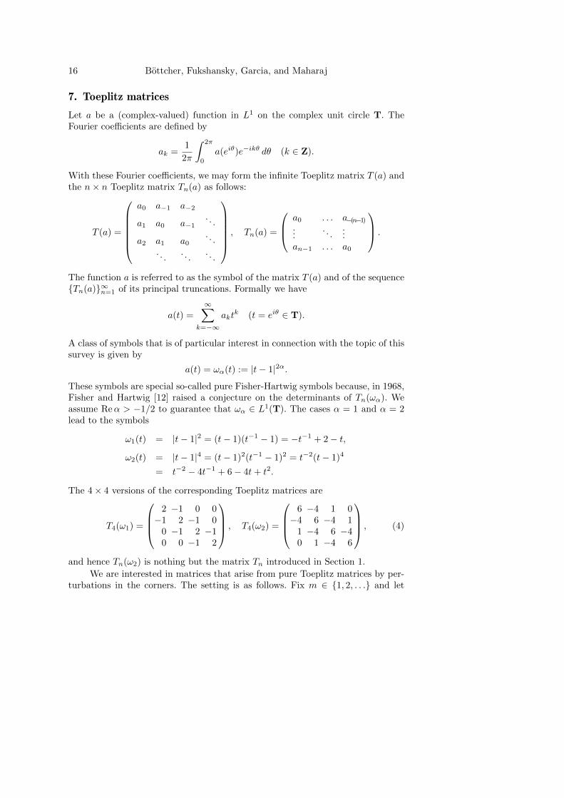
The 4× 4 versions of the corresponding Toeplitz matrices are
T4(ω1) =
2 −1 0 0−1 2 −1 0
0 −1 2 −10 0 −1 2
, T4(ω2) =
6 −4 1 0−4 6 −4 1
1 −4 6 −40 1 −4 6
, (4)
and hence Tn(ω2) is nothing but the matrix Tn introduced in Section 1.
We are interested in matrices that arise from pure Toeplitz matrices by per-turbations in the corners. The setting is as follows. Fix m ∈ {1, 2, . . .} and let
Lattice theory and Toeplitz determinants 17
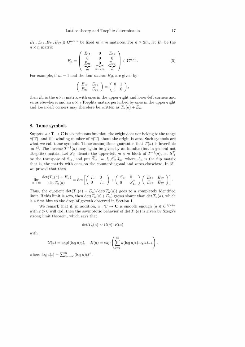
E11, E12, E21, E22 ∈ Cm×m be fixed m ×m matrices. For n ≥ 2m, let En be then× n matrix
En =
E11 0 E12
0 0 0E21︸︷︷︸m
0︸︷︷︸n−2m
E22︸︷︷︸m
∈ Cn×n. (5)
For example, if m = 1 and the four scalars Ejk are given by(E11 E12
E21 E22
)=
(0 11 0
),
then En is the n×n matrix with ones in the upper-right and lower-left corners andzeros elsewhere, and an n×n Toeplitz matrix perturbed by ones in the upper-rightand lower-left corners may therefore be written as Tn(a) + En.
8. Tame symbols
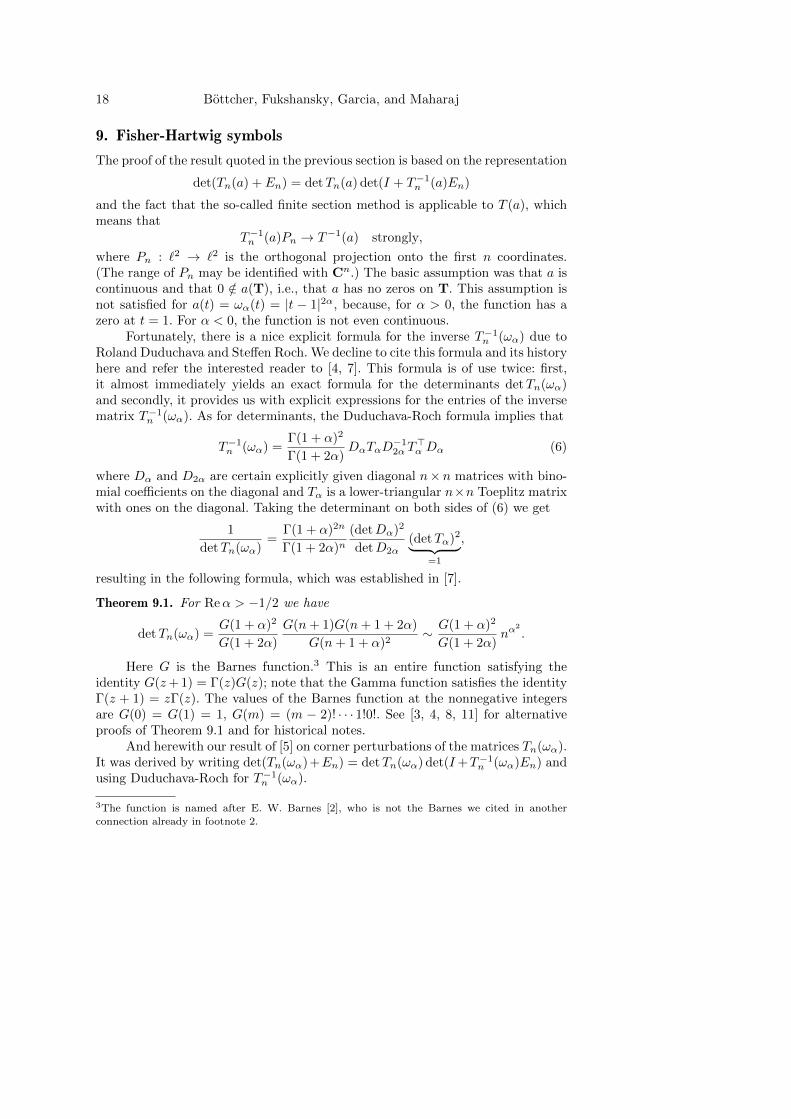
Suppose a : T→ C is a continuous function, the origin does not belong to the rangea(T), and the winding number of a(T) about the origin is zero. Such symbols arewhat we call tame symbols. These assumptions guarantee that T (a) is invertibleon `2. The inverse T−1(a) may again be given by an infinite (but in general notToeplitz) matrix. Let S11 denote the upper-left m × m block of T−1(a), let S>11be the transpose of S11, and put S>11 := JmS
>11Jm, where Jm is the flip matrix
that is, the matrix with ones on the counterdiagonal and zeros elsewhere. In [5],we proved that then
limn→∞
det(Tn(a) + En)
detTn(a)= det
[(Im 00 Im
)+
(S11 0
0 S>11
)(E11 E12
E21 E22
)].
Thus, the quotient det(Tn(a) + En)/ det(Tn(a)) goes to a completely identifiedlimit. If this limit is zero, then det(Tn(a)+En) grows slower than detTn(a), whichis a first hint to the drop of growth observed in Section 1.
We remark that if, in addition, a : T → C is smooth enough (a ∈ C1/2+ε
with ε > 0 will do), then the asymptotic behavior of detTn(a) is given by Szego’sstrong limit theorem, which says that
detTn(a) ∼ G(a)nE(a)
with
G(a) = exp((log a)0), E(a) = exp
( ∞∑k=1
k(log a)k(log a)−k
),
where log a(t) =∑∞k=−∞(log a)kt
k.
18 Bottcher, Fukshansky, Garcia, and Maharaj
9. Fisher-Hartwig symbols
The proof of the result quoted in the previous section is based on the representation
det(Tn(a) + En) = detTn(a) det(I + T−1n (a)En)
and the fact that the so-called finite section method is applicable to T (a), whichmeans that
T−1n (a)Pn → T−1(a) strongly,
where Pn : `2 → `2 is the orthogonal projection onto the first n coordinates.(The range of Pn may be identified with Cn.) The basic assumption was that a iscontinuous and that 0 /∈ a(T), i.e., that a has no zeros on T. This assumption isnot satisfied for a(t) = ωα(t) = |t − 1|2α, because, for α > 0, the function has azero at t = 1. For α < 0, the function is not even continuous.
Fortunately, there is a nice explicit formula for the inverse T−1n (ωα) due toRoland Duduchava and Steffen Roch. We decline to cite this formula and its historyhere and refer the interested reader to [4, 7]. This formula is of use twice: first,it almost immediately yields an exact formula for the determinants detTn(ωα)and secondly, it provides us with explicit expressions for the entries of the inversematrix T−1n (ωα). As for determinants, the Duduchava-Roch formula implies that
T−1n (ωα) =Γ(1 + α)2
Γ(1 + 2α)DαTαD
−12α T
>α Dα (6)
where Dα and D2α are certain explicitly given diagonal n×n matrices with bino-mial coefficients on the diagonal and Tα is a lower-triangular n×n Toeplitz matrixwith ones on the diagonal. Taking the determinant on both sides of (6) we get
1
detTn(ωα)=
Γ(1 + α)2n
Γ(1 + 2α)n(detDα)2
detD2α(detTα)2︸ ︷︷ ︸
=1
,
resulting in the following formula, which was established in [7].
Theorem 9.1. For Reα > −1/2 we have
detTn(ωα) =G(1 + α)2
G(1 + 2α)
G(n+ 1)G(n+ 1 + 2α)
G(n+ 1 + α)2∼ G(1 + α)2
G(1 + 2α)nα
2
.
Here G is the Barnes function.3 This is an entire function satisfying theidentity G(z+ 1) = Γ(z)G(z); note that the Gamma function satisfies the identityΓ(z + 1) = zΓ(z). The values of the Barnes function at the nonnegative integersare G(0) = G(1) = 1, G(m) = (m − 2)! · · · 1!0!. See [3, 4, 8, 11] for alternativeproofs of Theorem 9.1 and for historical notes.
And herewith our result of [5] on corner perturbations of the matrices Tn(ωα).It was derived by writing det(Tn(ωα)+En) = detTn(ωα) det(I+T−1n (ωα)En) andusing Duduchava-Roch for T−1n (ωα).
3The function is named after E. W. Barnes [2], who is not the Barnes we cited in anotherconnection already in footnote 2.
Lattice theory and Toeplitz determinants 19
Theorem 9.2. Let Reα > −1/2. If(E11 E12
E21 E22
)=
(0 11 0
)(7)
then
det(Tn(ωα) + En) ∼ G(1 + α)2
G(1 + 2α)2α(α+ 1)nα
2−1.
Comparing Theorems 9.1 and 9.2 we see that the corner perturbations (7) indeed
lower the growth of the determinants from nα2
to nα2−1. For α = 2, this is exactly
what we observed in Section 1.
In fact the exact expressions delivered by the Duduchava-Roch formula for theentries of T−1n (ωα) yield exact formulas for the determinants det(Tn(ωα) + En).Here are a few examples. We assume that the corner perturbations are of theform (7). Recall that Tn(ω1) and Tn(ω2) are the n×n analogues of the matrices (4).For these matrices,
detTn(ω1) = n+ 1 ∼ n, det(Tn(ω1) + En) = 4,
detTn(ω2) =(n+ 1)(n+ 2)2(n+ 3)
12∼ n4
12,
det(Tn(ω2) + En) = (n+ 1)3 ∼ n3.
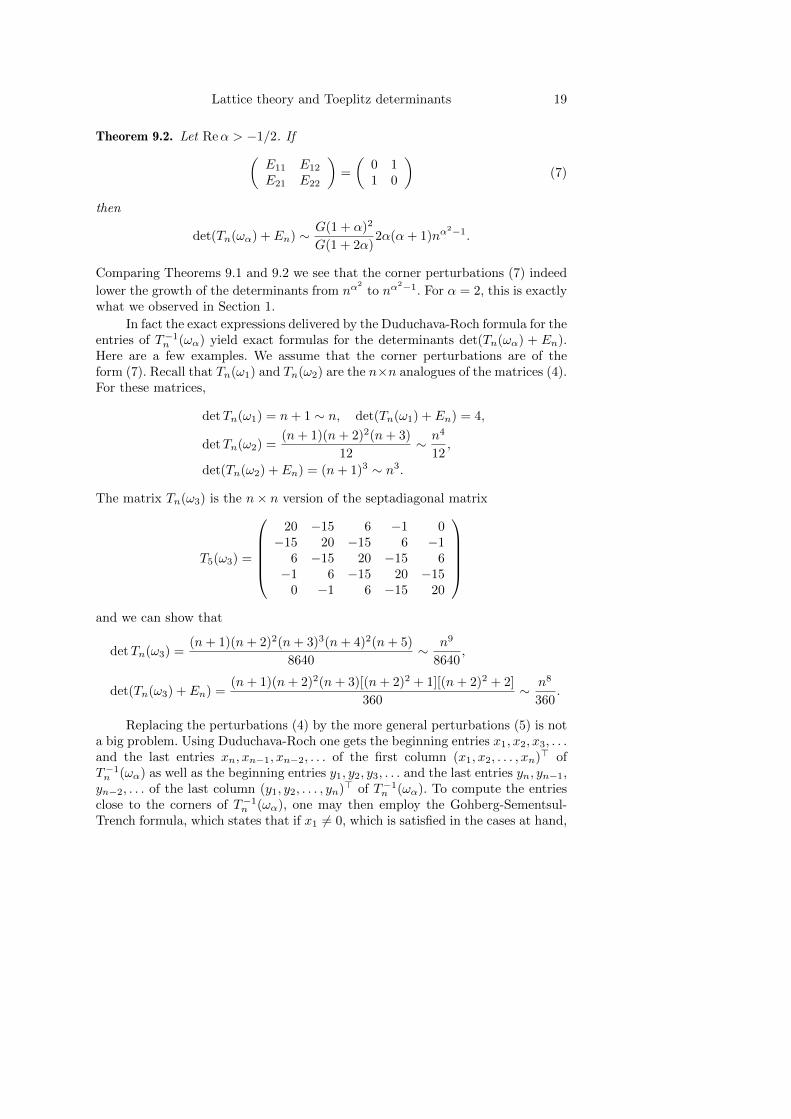
The matrix Tn(ω3) is the n× n version of the septadiagonal matrix
T5(ω3) =
20 −15 6 −1 0−15 20 −15 6 −1
6 −15 20 −15 6−1 6 −15 20 −15
0 −1 6 −15 20
and we can show that
detTn(ω3) =(n+ 1)(n+ 2)2(n+ 3)3(n+ 4)2(n+ 5)
8640∼ n9
8640,
det(Tn(ω3) + En) =(n+ 1)(n+ 2)2(n+ 3)[(n+ 2)2 + 1][(n+ 2)2 + 2]
360∼ n8
360.
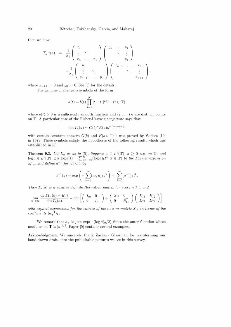
Replacing the perturbations (4) by the more general perturbations (5) is nota big problem. Using Duduchava-Roch one gets the beginning entries x1, x2, x3, . . .and the last entries xn, xn−1, xn−2, . . . of the first column (x1, x2, . . . , xn)> ofT−1n (ωα) as well as the beginning entries y1, y2, y3, . . . and the last entries yn, yn−1,yn−2, . . . of the last column (y1, y2, . . . , yn)> of T−1n (ωα). To compute the entriesclose to the corners of T−1n (ωα), one may then employ the Gohberg-Sementsul-Trench formula, which states that if x1 6= 0, which is satisfied in the cases at hand,
20 Bottcher, Fukshansky, Garcia, and Maharaj
then we have
T−1n (a) =1
x1
x1...
. . .
xn . . . x1
yn . . . y1
. . ....y1
− 1
x1
y0...
. . .
yn−1 . . . y0
xn+1 . . . x2
. . ....
xn+1
,
where xn+1 := 0 and y0 := 0. See [5] for the details.
The genuine challenge is symbols of the form
a(t) = b(t)
N∏j=1
|t− tj |2αj (t ∈ T)
where b(t) > 0 is a sufficiently smooth function and t1, . . . , tN are distinct pointson T. A particular case of the Fisher-Hartwig conjecture says that
detTn(a) ∼ G(b)nE(a)nα21+···+α
2N
with certain constant nonzero G(b) and E(a). This was proved by Widom [19]in 1973. These symbols satisfy the hypotheses of the following result, which wasestablished in [5].
Theorem 9.3. Let En be as in (5). Suppose a ∈ L1(T), a ≥ 0 a.e. on T, andlog a ∈ L1(T). Let log a(t) =
∑∞k=−∞(log a)kt
k (t ∈ T) be the Fourier expansion
of a, and define a−1+ for |z| < 1 by
a−1+ (z) = exp
(−∞∑k=1
(log a)kzk
)=:
∞∑k=0
(a−1+ )ktk.
Then Tn(a) is a positive definite Hermitian matrix for every n ≥ 1 and
limn→∞
det(Tn(a) + En)
detTn(a)= det
[(Im 00 Im
)+
(S11 0
0 S>11
)(E11 E12
E21 E22
)]with explicit expressions for the entries of the m ×m matrix S11 in terms of thecoefficients (a−1+ )k.
We remark that a+ is just exp(−(log a)0/2) times the outer function whosemodulus on T is |a|1/2. Paper [5] contains several examples.
Acknowledgment. We sincerely thank Zachary Glassman for transforming ourhand-drawn drafts into the publishable pictures we see in this survey.
Lattice theory and Toeplitz determinants 21
References
[1] E. S. Barnes, The perfect and extreme senary forms. Canad. J. Math. 9, 235–242(1957).
[2] E. W. Barnes, The theory of the G-function. The Quarterly Journal of Pure andApplied Mathematics 31, 264–314 (1900).
[3] E. Basor and Y. Chen, Toeplitz determinants from compatibility conditions. Ramanu-jan J. 16, 25–40 (2008).
[4] A. Bottcher, The Duduchava-Roch formula. Operator Theory: Advances and Appli-cations (The Roland Duduchava Anniversary Volume), to appear.
[5] A. Bottcher, L. Fukshansky, S. R. Garcia, and H. Maharaj, Toeplitz determinantswith perturbations in the corners. J. Funct. Anal. 268, 171–193 (2015).
[6] A. Bottcher, L. Fukshansky, S. R. Garcia, and H. Maharaj, On lattices generated byfinite Abelian groups. SIAM J. Discrete Math. 29, 382–404 (2015).
[7] A. Bottcher and B. Silbermann, Toeplitz matrices and determinants with Fisher-Hartwig symbols. J. Funct. Analysis 63, 178–214 (1985).
[8] A. Bottcher and H. Widom, Two elementary derivations of the pure Fisher-Hartwigdeterminant. Integral Equations Operator Theory 53, 593–596 (2005).
[9] J. H. Conway and N. J. A. Sloane, A lattice without a basis of minimal vectors.Mathematika 42, 175–177 (1995).
[10] J. H. Conway and N. J. A. Sloane, Sphere Packings, Lattices, and Groups. Thirdedition, Springer-Verlag, New York 1999.
[11] P. Deift, A. Its, and I. Krasovsky, Toeplitz matrices and Toeplitz determinants underthe impetus of the Ising model. Some history and some recent results. Commun. Pureand Appl. Math. 66, 1360–1438 (2013).
[12] M. E. Fisher and R. E. Hartwig, Toeplitz determinants - some applications, theorems,and conjectures. Adv. Chem. Phys. 15, 333–353 (1968).
[13] L. Fukshanky and H. Maharaj, Lattices from elliptic curves over finite fields. FiniteFields Appl. 28, 67–78 (2014).
[14] J. Martinet and A. Schurmann, Bases of minimal vectors in lattices, III. Int. J.Number Theory 8, 551–567 (2012).
[15] H.-G. Ruck, A note on elliptic curves over finite fields. Math. Comp. 49, 301–304(1987).
[16] M. Sha, On the lattices from ellptic curves over finite fields. Finite Fields Appl. 31,84–107 (2015).
[17] H. Stichtenoth, Algebraic Function Fields and Codes. 2nd edition, Springer-Verlag,Berlin 2009.
[18] M. A. Tsfasman and S. G. Vladut, Algebraic-Geometric Codes. Kluwer AcademicPublishers, Dordrecht 1991.
[19] H. Widom, Toeplitz determinants with singular generating functions. Amer. J. Math.95, 333–383 (1973).
22 Bottcher, Fukshansky, Garcia, and Maharaj
Albrecht BottcherFakultat fur Mathematik, Technische Universitat Chemnitz, 09107 Chemnitz, Germanye-mail: [email protected]
Lenny FukshanskyDepartment of Mathematics, Claremont McKenna College, 850 Columbia Ave, Clare-mont, CA 91711, USAe-mail: [email protected]
Stephan Ramon Garcia,Department of Mathematics, Pomona College, 610 N. College Ave, Claremont, CA 91711,USAe-mail: [email protected]
Hiren MaharajDepartment of Mathematics, Pomona College, 610 N. College Ave, Claremont, CA 91711,USAe-mail: [email protected]