Lattice Point Geometry: Pick’s Theorem andMinkowski’s Theorem

Senior Exercise in Mathematics

Jennifer GarbettKenyon College

November 18, 2010

Contents

1 Introduction 1

2 Primitive Lattice Triangles 52.1 Triangulation of a Lattice Polygon with Lattice Triangles . . . . . . . . . . 52.2 Triangulation of a Lattice Polygon with Primitive Lattice Triangles . . . . 72.3 Visible Points . . . . . . . . . . . . . . . . . . . . . . . . . . . . . . . . . . 102.4 Plane Isometry . . . . . . . . . . . . . . . . . . . . . . . . . . . . . . . . . 122.5 Primitive Parallelograms . . . . . . . . . . . . . . . . . . . . . . . . . . . . 122.6 The Area of a Primitive Lattice Triangle . . . . . . . . . . . . . . . . . . . 15

3 Pick’s Theorem 163.1 Basic Definitions From Graph Theory . . . . . . . . . . . . . . . . . . . . . 163.2 Proving Pick’s Theorem . . . . . . . . . . . . . . . . . . . . . . . . . . . . 183.3 Beyond Pick’s Theorem . . . . . . . . . . . . . . . . . . . . . . . . . . . . 22

3.3.1 Pick’s Theorem for Non-Simple Polygons . . . . . . . . . . . . . . . 223.3.2 Pick’s Theorem for Polygons kP . . . . . . . . . . . . . . . . . . . . 25

4 Convex Regions in R2 29

5 Minkowski’s Theorem 315.1 Proving Minkowski’s Theorem . . . . . . . . . . . . . . . . . . . . . . . . . 335.2 Minkowski’s Theorem in an Arbitrary Lattice . . . . . . . . . . . . . . . . 345.3 Applications of Minkowski’s Theorem . . . . . . . . . . . . . . . . . . . . . 37

5.3.1 The Two Squares Theorem . . . . . . . . . . . . . . . . . . . . . . . 385.3.2 The Orchard Problem . . . . . . . . . . . . . . . . . . . . . . . . . 40

6 Minkowski’s Theorem in Rn 416.1 Proving Minkowski’s Theorem in Rn . . . . . . . . . . . . . . . . . . . . . 416.2 Applications of Minkowski’s Theorem in Rn . . . . . . . . . . . . . . . . . 43

7 Conclusions 43

8 Acknowledgements 43

1 Introduction

Informally, a lattice is a “set of isolated points”, one of which is the origin, and this “pointset... looks the same no matter from which of its points you observe it” [8]. The study oflattices is interesting on its own and has lead to solutions to problems in other branches ofmathematics.

Our main goal here will be to discuss two theorems based in lattice point geometry,Pick’s Theorem and Minkowski’s Theorem. Both theorems allow us to describe the re-lationships between the area of a polygon in the plane and the number of lattice pointsthe polygon contains, both extend to higher dimensions, and both have important appli-cations, ranging from solutions to applied problems to proofs of important theorems innumber theory.

Let L be a lattice and let P be a polygon in the plane with its vertices at points inL. Pick’s Theorem allows us to determine the area of P based on the number of latticepoints, points in L, living inside P and the number of lattice points living on the boundaryof P . Minkowski’s Theorem allows us to go in the other direction. Let R be a regionin R2. Minkowski’s Theorem guarantees R contains a lattice point if R satisfies a set ofrequirements set forth by the theorem.

We will discuss Pick’s Theorem and Minkowski’s Theorem more after a brief introduc-tion to lattices. We will then give an overview of the steps we will need to take to provePick’s Theorem and Minkowski’s Theorem. We will follow this introductory material withthe bulk of the paper, a detailed discussion of the results required to prove Pick’s Theoremand Minkowski’s Theorem as well as a discussion of the consequences of these two theorems.

Before we get into the details of the main theorems of the paper, we need to addressthe definition of a lattice in more detail. First, we give a more formal definition of a lattice[8]:

Definition 1.1. A set, L, of points in Rn is a lattice if it satisfies the following conditions:

1. L is a group under vector addition.

2. Each point in L is the center of a ball that contains no other points of L.

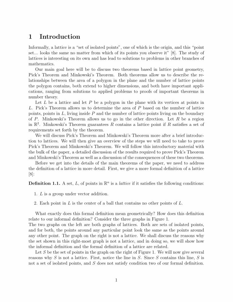
What exactly does this formal definition mean geometrically? How does this definitionrelate to our informal definition? Consider the three graphs in Figure 1.The two graphs on the left are both graphs of lattices. Both are sets of isolated points,and for both, the points around any particular point look the same as the points aroundany other point. The graph on the right is not a lattice. We shall discuss the reasons whythe set shown in this right-most graph is not a lattice, and in doing so, we will show howthe informal definition and the formal definition of a lattice are related.

Let S be the set of points in the graph on the right of Figure 1. We will now give severalreasons why S is not a lattice. First, notice the line in S. Since S contains this line, S isnot a set of isolated points, and S does not satisfy condition two of our formal definition.

1

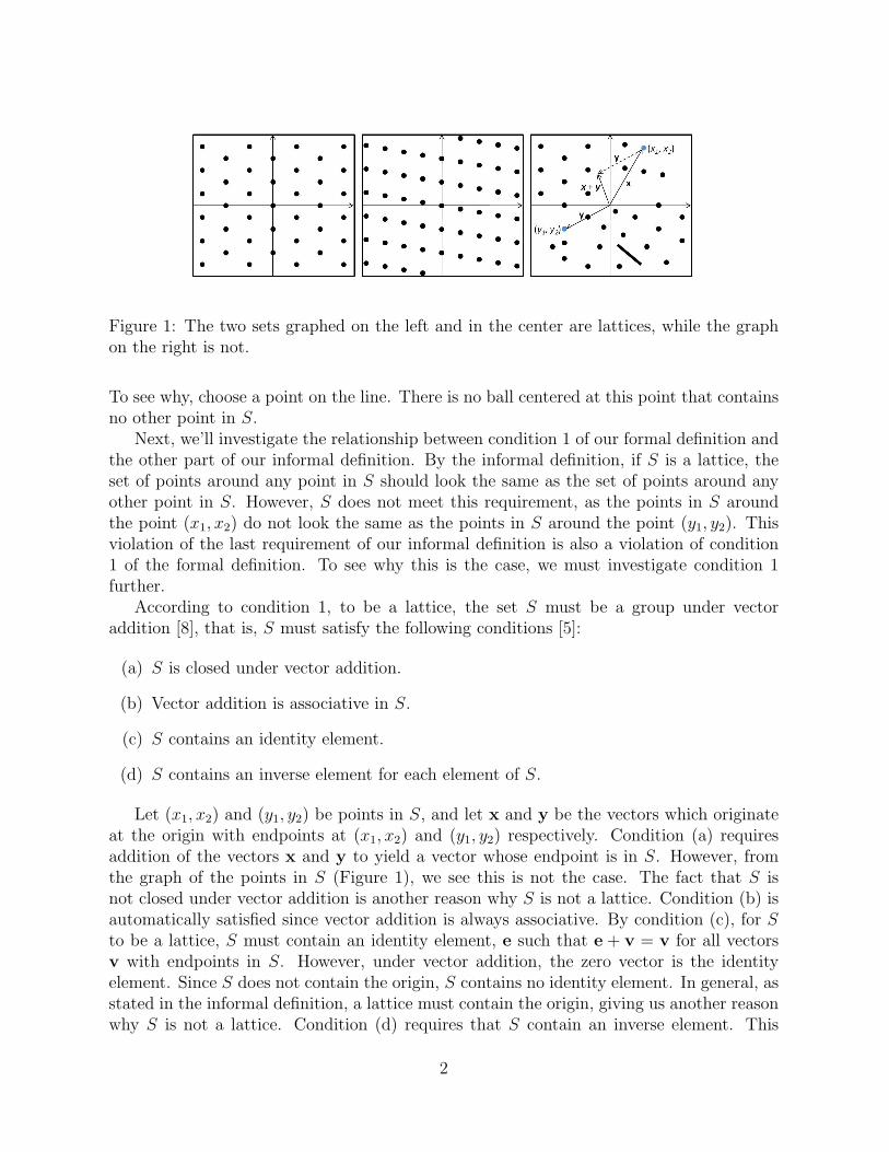
Figure 1: The two sets graphed on the left and in the center are lattices, while the graphon the right is not.

To see why, choose a point on the line. There is no ball centered at this point that containsno other point in S.

Next, we’ll investigate the relationship between condition 1 of our formal definition andthe other part of our informal definition. By the informal definition, if S is a lattice, theset of points around any point in S should look the same as the set of points around anyother point in S. However, S does not meet this requirement, as the points in S aroundthe point (x1, x2) do not look the same as the points in S around the point (y1, y2). Thisviolation of the last requirement of our informal definition is also a violation of condition1 of the formal definition. To see why this is the case, we must investigate condition 1further.

According to condition 1, to be a lattice, the set S must be a group under vectoraddition [8], that is, S must satisfy the following conditions [5]:

(a) S is closed under vector addition.

(b) Vector addition is associative in S.

(c) S contains an identity element.

(d) S contains an inverse element for each element of S.

Let (x1, x2) and (y1, y2) be points in S, and let x and y be the vectors which originateat the origin with endpoints at (x1, x2) and (y1, y2) respectively. Condition (a) requiresaddition of the vectors x and y to yield a vector whose endpoint is in S. However, fromthe graph of the points in S (Figure 1), we see this is not the case. The fact that S isnot closed under vector addition is another reason why S is not a lattice. Condition (b) isautomatically satisfied since vector addition is always associative. By condition (c), for Sto be a lattice, S must contain an identity element, e such that e + v = v for all vectorsv with endpoints in S. However, under vector addition, the zero vector is the identityelement. Since S does not contain the origin, S contains no identity element. In general, asstated in the informal definition, a lattice must contain the origin, giving us another reasonwhy S is not a lattice. Condition (d) requires that S contain an inverse element. This

2

is impossible since S contains no identity element. Had S contained an identity element,the origin, we would need to check whether for every point p in S, −p is in S. We wouldneed S to satisfy this condition because the inverse of a point p under vector addition is−p since p − p = 0 where p is the vector emanating from the origin with endpoint p.Since S doesn’t contain an inverse for every point in S, S violates all of the conditions setout in our formal definition of a lattice other than part (b) of condition one. A set is nota lattice if it violates even one of the conditions or subconditions set forth in our formaldefinition. Only a set of points that satisfies all of the conditions of our formal definitionis a lattice, and the sets plotted in the two graphs on the left of Figure 1 do satisfy all ofthese conditions and are therefore lattices.

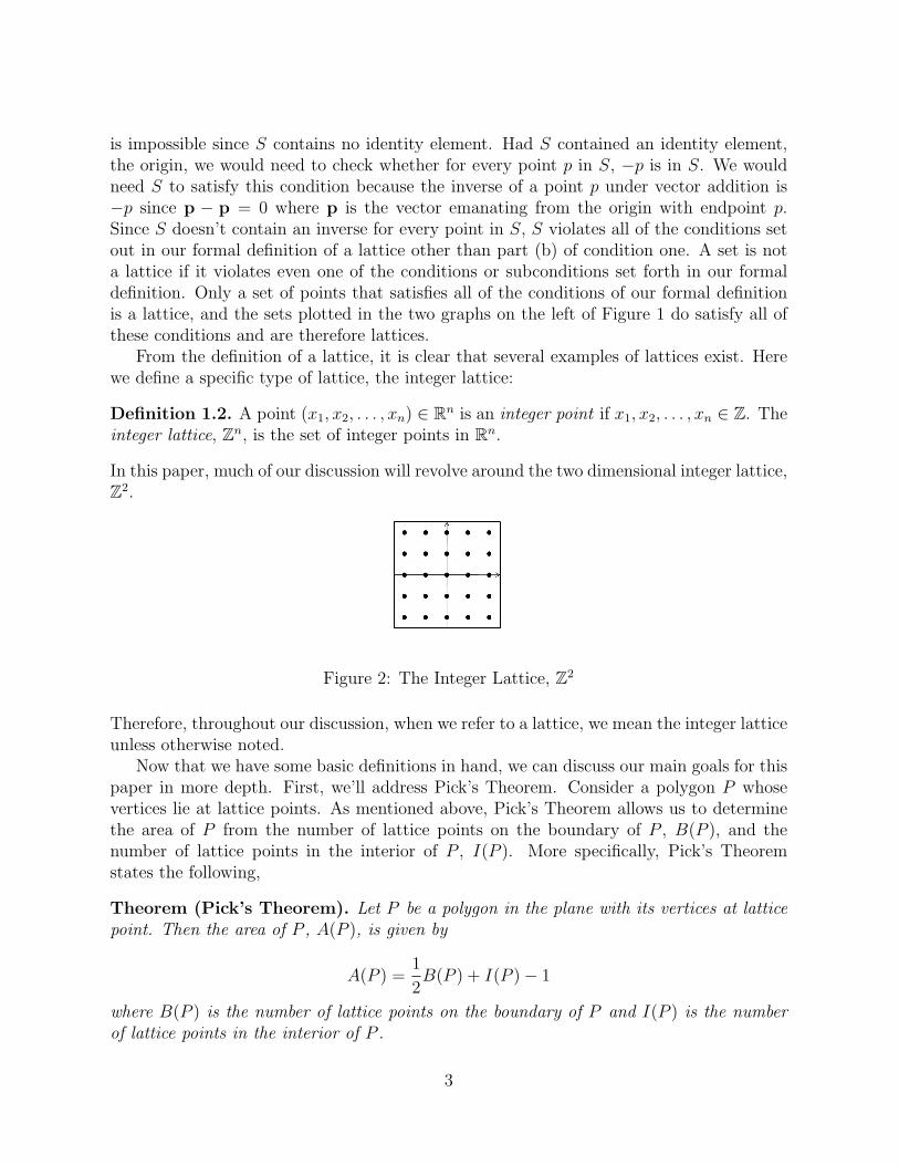
From the definition of a lattice, it is clear that several examples of lattices exist. Herewe define a specific type of lattice, the integer lattice:

Definition 1.2. A point (x1, x2, . . . , xn) ∈ Rn is an integer point if x1, x2, . . . , xn ∈ Z. Theinteger lattice, Zn, is the set of integer points in Rn.

In this paper, much of our discussion will revolve around the two dimensional integer lattice,Z2.

Figure 2: The Integer Lattice, Z2

Therefore, throughout our discussion, when we refer to a lattice, we mean the integer latticeunless otherwise noted.

Now that we have some basic definitions in hand, we can discuss our main goals for thispaper in more depth. First, we’ll address Pick’s Theorem. Consider a polygon P whosevertices lie at lattice points. As mentioned above, Pick’s Theorem allows us to determinethe area of P from the number of lattice points on the boundary of P , B(P ), and thenumber of lattice points in the interior of P , I(P ). More specifically, Pick’s Theoremstates the following,

Theorem (Pick’s Theorem). Let P be a polygon in the plane with its vertices at latticepoint. Then the area of P , A(P ), is given by

A(P ) =1

2B(P ) + I(P )− 1

where B(P ) is the number of lattice points on the boundary of P and I(P ) is the numberof lattice points in the interior of P .

3

To prove Pick’s Theorem, we’ll first divide the polygon P into triangles each with area12; proving that this is possible will complete much of the preliminary work necessary to

prove Pick’s Theorem. Then, we will introduce some basic definitions and establish a fewfacts from graph theory. This knowledge of some elementary graph theory will allow us totreat the polygon, P , which we divided into triangles of area 1

2, as a graph. Doing so will

allow us to determine how many triangles with area 12

P contains in terms of B(P ) andI(P ). After we accomplish all of these tasks, we will be able to derive the formula givenby Pick’s Theorem for the area of P .

There are several extensions of Pick’s Theorem in the plane. We will discuss a few ofthese extensions in detail. Those we will discuss in detail include the following. First, wewill discuss a version of Pick’s Theorem for polygons containing holes (we will see thatPick’s Theorem does not apply to polygons containing holes)[9]. Next, we will discuss aversion of Pick’s Theorem that allows us to determine the number of lattice points in apolygon kP = {kx|x ∈ P}, where P is a lattice polygon, for all positive integers k [6].Finally, we will discuss a version of Pick’s Theorem that allows us to find an upper boundfor the number of lattice points in a non-polygonal region in R2 [6]. To discuss this lastextension of Pick’s Theorem, we will need to discuss convexity in R2. This discussionof convexity in the plane will lead us to the next major topic of the paper, Minkowski’sTheorem.

While our final extension of Pick’s Theorem will give us an upper bound on the numberof lattice points in a region in R2, Minkowski’s Theorem will allow us to determine whetherwe are guaranteed to find more than one lattice point in a region in R2. Minkowski’sTheorem is as follows,

Theorem (Minkowski’s Theorem). Let R be a bounded, convex region in R2 havingarea greater than 4 that is symmetric about the origin. Then R contains an integer pointother than the origin.

We will discuss Minkowski’s Theorem and its requirements (convexity, symmetry, etc.)in sections 4 and 5. If Minkowski’s Theorem guarantees the existence of a lattice point ina region R besides the origin, then we have a lower bound of two for the number of latticepoints in R. Thus, both Pick’s Theorem and Minkowski’s Theorem give us informationabout regions in the plane based on numbers we can find easily, such as the number oflattice points in the interior of the region, the number of lattice points on the boundaryof the region, the area of the region, or the perimeter of the region. We now give a briefoverview of Minkowski’s Theorem.

We won’t need many new results to prove Minkowski’s Theorem. First we’ll proveBlichfeldt’s lemma which guarantees any bounded set in R2 with area greater than 1 willcontain two distinct points whose difference under vector addition is an integer point. Wewill use this result to show a larger region, a region that satisfies the requirements ofMinkowski’s Theorem, must contain an integer point.

As we will do for Pick’s Theorem, we will also discuss some of the many extensions ofMinkowski’s Theorem; we’ll also discuss a couple of applications of Minkowski’s Theorem.First, we will discuss Minkowski’s Theorem in lattices other than the integer lattice [2].

4

Next we’ll discuss two applications of Minkwoski’s Theorem. As mentioned previously,Minkowski’s Theorem can be used in the proofs of some important theorems in numbertheory. We will discuss and prove one such theorem, the Two Squares Theorem, for aparticular case. The Two Squares Theorem tells us which integers can be written as a sumof two squares and which cannot [2]. We will use Minkowski’s Theorem to show whichprimes can be written as a sum of two squares, proving the Two Squares Theorem forprime numbers. Minkowski’s Theorem can also be used in solving the Orchard Problem,an applied problem involving a circular orchard of trees planted at lattice points [3]. We willconclude our discussion of Minkowski’s Theorem with a proof of an extension of Minkowski’sTheorem to regions in Rn followed by a brief discussion of a few important applications ofMinkowski’s Theorem in Rn. Throughout the paper, all theorems, definitions, proofs, etc.are adapted from [6] unless otherwise noted.

2 Primitive Lattice Triangles

As mentioned above, our proof of Pick’s theorem will hinge on the fact that every polygonwith its vertices at lattice points can be divided into triangles. Each triangle has all threeof its vertices at lattice points and has area 1

2. Once we complete this section, we will have

shown we can divide any polygon P , with all of its vertices at lattice points, into trianglesall of the same known area, 1

2.

2.1 Triangulation of a Lattice Polygon with Lattice Triangles

Up to now, we’ve simply said Pick’s Theorem will give us a way to determine the area of apolygon with its vertices at lattice points. Before we proceed further, we clarify the specificcharacteristics a polygon must have for the formula given in Pick’s Theorem to determineits area. To use Pick’s Theorem to determine the area of a polygon, P , P must be a simplelattice polygon.

Definition 2.1. A simple polygon, P , is a polygon whose boundary is a simple closedcurve, that is, P contains no holes, and the boundary of P never intersects itself [9]. Alattice polygon is a polygon, not necessarily simple, with all its vertices at lattice points. Asimple lattice polygon is a simple polygon with all its vertices at lattice points.

These definitions give rise to a few issues regarding notation. When we refer to a latticepolygon, we assume it is a simple lattice polygon unless noted otherwise. Also, we refer toa polygon P with k vertices as a k-gon,

Our first step towards a proof of Pick’s theorem is to show we can dissect any latticepolygon into lattice triangles.

Definition 2.2. We call the dissection of a polygon P into triangles a triangulation of P .

To show we can triangulate any polygon, P , even if P is non-simple, we’ll first need toshow that P must have a diagonal.

5

Definition 2.3. Let P be a polygon which need not be simple. Let l be a line segmentcontained in P that joins two non-adjacent vertices of P . If l does not contain any vertexof P other than the two it connects, then the line segment l is a diagonal of P .

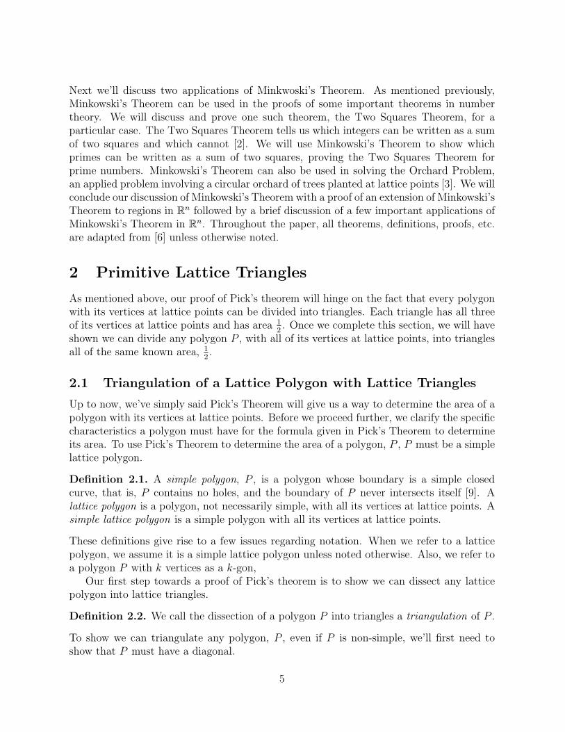
Lemma 2.4. Every polygon, P , where P need not be a simple lattice polygon, has a diag-onal.

Proof. Let P be a polygon having k vertices, and graph the polygon P in R2. Call thevertices of P (x1, y1), (x2, y2), . . . , (xk, yk). Let l be the line y = min{yi|1 ≤ i ≤ k}. Thenno vertex of P lies below l. Choose a vertex of P that lies on l, and call it A. Let B andC be the vertices of P adjacent to A. We must consider three cases (see Figure 3).

1. Assume the line segment BC is a diagonal of P . Then P has a diagonal and we’redone (see Figure 3).

2. Assume some vertex of P lies on BC, but no vertex of P lies inside 4ABC. Choosea vertex of P on BC and call it V . Then AV is a diagonal of P (see Figure 3).

3. Assume some vertex of P lies inside 4ABC. Choose a vertex of P that lies inside4ABC, and call it V . Draw a line segment, s with one endpoint at A and the otheron BC that passes through V . If V is the only vertex of P on s, then AV is a diagonalof P . If there is more than one vertex of P on s, let X be the one that lies closest toA. Then AX is a diagonal of P (see Figure 3).

Figure 3: Case 1: BC is a diagonal of P . Case 2: A vertex of P lies on BC. Case 3: Avertex of P lies inside 4ABC

Thus, every polygon, P must have a diagonal.

Given this result, proving any polygon, P , can be dissected into triangles each of whichhas vertices that are vertices of P becomes a simple exercise in mathematical induction.

Theorem 2.5. Every k-gon, Pk, can be dissected into k − 2 triangles, each of which hasvertices that are vertices of Pk, by means of nonintersecting diagonals.

Proof. We proceed by complete induction on k. Since Pk is not a polygon when k < 3, weconsider k ≥ 3. For the base case, assume k = 3. Since P3 is a triangle, the theorem is truewhen k = 3. Let k > 3 and assume all polygons with k vertices or less satisfy the theorem.We must show a polygon with k + 1 vertices satisfies the theorem.

6

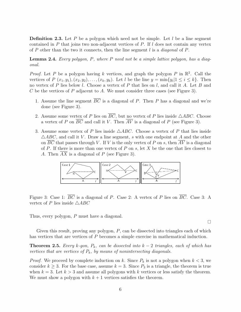
By Lemma 2.4, Pk+1 must have a diagonal, d. The diagonal d splits Pk+1 into two smallerpolygons, Pm which has m vertices and Pn which has n vertices (see figure 4). Since eachof the two smaller polygons, Pm and Pn, contains the endpoints of d as two of its vertices,m+n gives us two more than number of vertices of Pk+1, that is, m+n = (k+1)+2. Since3 ≤ m ≤ k and 3 ≤ n ≤ k, by our induction hypothesis, Pm and Pn satisfy the theorem;they can be dissected into m−2 and n−2 triangles, respectively. Each vertex of each trianglelies at a vertex of P . Since the diagonals of Pm must be inside Pm, the diagonals of Pn

must be inside Pn, and Pm and Pn are disjoint and separated by d, no diagonal of Pm or Pn

intersects d. Therefore, the nonintersecting diagonals of Pm, the nonintersecting diagonalsof Pn, and d dissect Pk+1 into (m−2)+(n−2) = (m+n)−4 = ((k+1)+2)−4 = (k+1)−2triangles as stated in the theorem. Thus, every k-gon can be dissected into k − 2 trianglesas stated by the theorem.

Figure 4: The polygon Pk+1 is divided by a diagonal, d, into two smaller polygons, Pm andPn, each of which can be triangulated (dotted lines) as in the theorem.

We’ve shown any polygon, P , can be triangulated with triangles each of which hasvertices that are vertices of P . If P is a lattice polygon, all of its vertices are at latticepoints. Since we can triangulate P with triangles whose vertices are at vertices of P , allof the vertices of the triangles with which we triangulate P are at lattice points. Thus,Corollary ?? follows directly from Theorem 2.5.

Corollary 2.6. Every lattice polygon, P can be dissected into lattice triangles whose verticesare vertices of P .

Corollary 2.6 allows us to triangulate any lattice polygon with lattice triangles. However,to prove Pick’s theorem, we’ll need a stronger result; as mentioned before, we need to showany lattice polygon can be triangulated with triangles each of which has an area of 1

2.

2.2 Triangulation of a Lattice Polygon with Primitive LatticeTriangles

In this section we will show we can triangulate a lattice polygon with a particular type oftriangle, a primitive lattice triangle.

7

Definition 2.7. A primitive lattice polygon is a lattice polygon with no lattice points inits interior and with no lattice points on its sides other than its vertices.

In this section, we are concerned with primitive lattice triangles. A primitive lattice triangleis a triangle with no lattice points in its interior and with no lattice points on its sides otherthan its vertices. We will defer showing the area of a primitive triangle must be 1

2to the

following sections. Here, we show triangulation with primitive lattice triangles is possible.

Theorem 2.8. Every lattice polygon can be dissected into primitive lattice triangles.

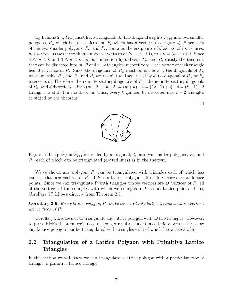
Proof. Let P be a lattice polygon. By Corollary 2.6 we can triangulate P with latticetriangles. Therefore, it is sufficient to show a lattice triangle can be triangulated withprimitive lattice triangles. Let Tr = 4ABC be a lattice triangle with a finite number,r ≥ 0, of lattice points in its interior. If Tr is primitive, then we’re done. Assume Tr is notprimitive. We proceed by complete induction on r. We have two base cases.

First, let r = 0. Since there are no lattice points inside T0 and T0 is not primitive, theremust be at least one lattice point on the boundary of T0. Without loss of generality, assumethat this lattice point, or at least one lattice point if there are multiple lattice points onthe boundary of T0, lies on AB. Call the lattice points on AB X1, X2, . . . , Xk. The linesegments CX1, CX2, . . . , CXk dissect T0 into triangles. Since there are no lattice pointsinside T0, all of the triangles formed by CX1, CX2, . . . , CXk are primitive except possibly4ACX1 and 4CBXk. Assume there are no lattice points on AC and there are no latticepoints on CB. Then 4ACX1 and 4CBXk are primitive, and we’re done. Assume thereare lattice points Y1, Y2, . . . , Ym on AC. Since T0 contains no interior lattice points, 4ACX1

contains no interior lattice points, and therefore, the line segments X1Y1, X1Y2, . . . , X1Ym

divide 4ACX1 into primitive lattice triangles. The same argument holds when there arelattice points on CB. Thus, T0 can be triangulated with primitive lattice triangles (seeFigure 5).

Figure 5: A triangulation of T0 with primitive triangles

8

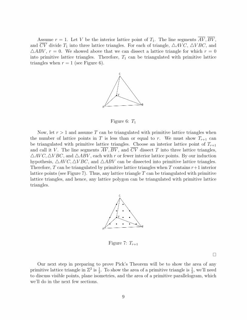
Assume r = 1. Let V be the interior lattice point of T1. The line segments AV , BV ,and CV divide T1 into three lattice triangles. For each of triangle, 4AV C, 4V BC, and4ABV , r = 0. We showed above that we can dissect a lattice triangle for which r = 0into primitive lattice triangles. Therefore, T1 can be triangulated with primitive latticetriangles when r = 1 (see Figure 6).

Figure 6: T1

Now, let r > 1 and assume T can be triangulated with primitive lattice triangles whenthe number of lattice points in T is less than or equal to r. We must show Tr+1 canbe triangulated with primitive lattice triangles. Choose an interior lattice point of Tr+1

and call it V . The line segments AV , BV , and CV dissect T into three lattice triangles,4AV C,4V BC, and 4ABV , each with r or fewer interior lattice points. By our inductionhypothesis, 4AV C,4V BC, and 4ABV can be dissected into primitive lattice triangles.Therefore, T can be triangulated by primitive lattice triangles when T contains r+1 interiorlattice points (see Figure 7). Thus, any lattice triangle T can be triangulated with primitivelattice triangles, and hence, any lattice polygon can be triangulated with primitive latticetriangles.

Figure 7: Tr+1

Our next step in preparing to prove Pick’s Theorem will be to show the area of anyprimitive lattice triangle in Z2 is 1

2. To show the area of a primitive triangle is 1

2, we’ll need

to discuss visible points, plane isometries, and the area of a primitive parallelogram, whichwe’ll do in the next few sections.

9

2.3 Visible Points

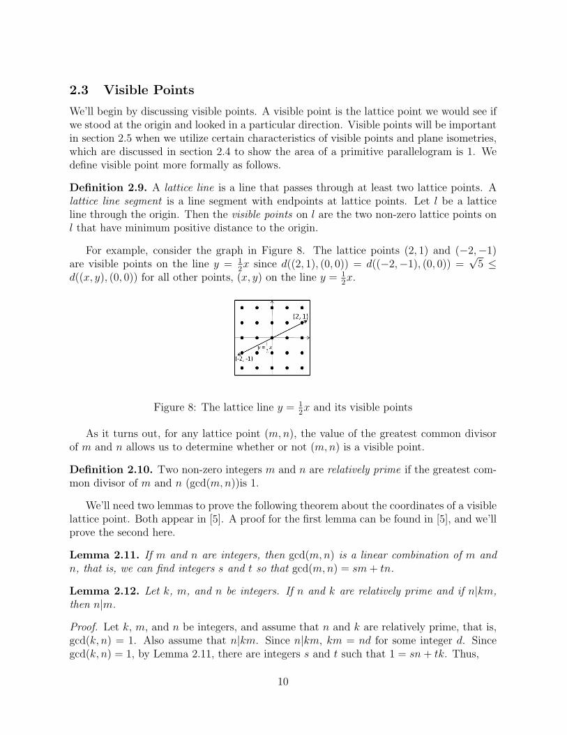
We’ll begin by discussing visible points. A visible point is the lattice point we would see ifwe stood at the origin and looked in a particular direction. Visible points will be importantin section 2.5 when we utilize certain characteristics of visible points and plane isometries,which are discussed in section 2.4 to show the area of a primitive parallelogram is 1. Wedefine visible point more formally as follows.

Definition 2.9. A lattice line is a line that passes through at least two lattice points. Alattice line segment is a line segment with endpoints at lattice points. Let l be a latticeline through the origin. Then the visible points on l are the two non-zero lattice points onl that have minimum positive distance to the origin.

For example, consider the graph in Figure 8. The lattice points (2, 1) and (−2,−1)are visible points on the line y = 1

2x since d((2, 1), (0, 0)) = d((−2,−1), (0, 0)) =

√5 ≤

d((x, y), (0, 0)) for all other points, (x, y) on the line y = 12x.

Figure 8: The lattice line y = 12x and its visible points

As it turns out, for any lattice point (m,n), the value of the greatest common divisorof m and n allows us to determine whether or not (m,n) is a visible point.

Definition 2.10. Two non-zero integers m and n are relatively prime if the greatest com-mon divisor of m and n (gcd(m, n))is 1.

We’ll need two lemmas to prove the following theorem about the coordinates of a visiblelattice point. Both appear in [5]. A proof for the first lemma can be found in [5], and we’llprove the second here.

Lemma 2.11. If m and n are integers, then gcd(m, n) is a linear combination of m andn, that is, we can find integers s and t so that gcd(m, n) = sm + tn.

Lemma 2.12. Let k, m, and n be integers. If n and k are relatively prime and if n|km,then n|m.

Proof. Let k, m, and n be integers, and assume that n and k are relatively prime, that is,gcd(k, n) = 1. Also assume that n|km. Since n|km, km = nd for some integer d. Sincegcd(k, n) = 1, by Lemma 2.11, there are integers s and t such that 1 = sn + tk. Thus,

10

m = m(sn + tk)

= smn + tkm

= smn + tnd

= n(sm + td).

Since s, m, t, and d are all integers, sm + td is an integer, so n|m.

Theorem 2.13. A lattice point p = (m, n) is visible if and only if m and n are relativelyprime.

Proof. We must show two implications.

(=⇒) Let p = (m, n) be a visible point, and let s be a the lattice line segment with endpointsat the origin and p. Then there is no lattice point on s other than its endpoints.Assume m and n are not relatively prime, that is, gcd(m,n) = k > 1. It follows thatmk

and nk

are integers, and since s is a segment of the lattice line y = nm

x, the latticepoint (m

k, n

k) lies on s. This means the point (m

k, n

k) lies between the point p and the

origin, contradicting the fact that (m,n) is a visible point. Thus, gcd(m, n) = 1, andtherefore, m and n are relatively prime.

(⇐=) Assume m and n are relatively prime, that is, gcd(m, n) = 1. Let s be the latticeline segment with endpoints at (0, 0) and p = (m, n). Let q = (m′, n′) be a non-zerolattice point on s. To show p is visible, we must show q = p. We do so by consideringthree cases.

1. Assume m′ = 0. Then s must be a vertical line. This means p = (0, n). Sincegcd(m, n) = 1, n = 1, and since q is a non-zero lattice point on s, n′ = 1. Thus,q = p.

2. Assume n′ = 0. Then s must be a horizontal line. This means p = (m, 0). Sincegcd(m, n) = 1, m = 1, and since q is a non-zero lattice point on s, m′ = 1. Thus,q = p.

3. Now assume that m′ 6= 0 and n′ 6= 0. Since p and q both lie on s, the slopeof s is n

m= n′

m′ . Since nm

= n′

m′ , mn′ = m′n, and thus, m|m′n. By Lemma2.12, since m|m′n and since m and n are relatively prime, m|m′. Similarly,mn′ = m′n =⇒ n|mn′. Also by Lemma 2.12, n|n′. Since q is on the linesegment s, it must be the case that |m′| ≤ |m| and |n′| ≤ |n|. Therefore, sincem′, n′ ∈ Z, m′ = m and n′ = n. Thus, q = p.

11

This relationship between the greatest common divisor of the coordinates of a pointand whether or not the point is a visible point will be necessary in the steps leading up toshowing the area of a primitive lattice triangle is 1

2. As mentioned above, we will combine

the result of Theorem 2.13 with characteristics of plane isometries to show the area of aprimitive lattice parallelogram is 1.

2.4 Plane Isometry

The information about plane isometries presented here is from [5]. An understanding ofplane isometries will allow us to employ functions to move lattice polygons within a latticewhile ensuring the area of the polygon does not change. This is important since we areinterested in the areas of lattice polygons, and it is often easier to calculate the area of apolygon when we know its location in the plane.

Definition 2.14. A plane isometry is a distance preserving function ϕ : R2 → R2. Thatis, for all points x = (x1, x2) and y = (y1, y2) in R2, ||ϕ(x)−ϕ(y)|| = ||x−y|| where ||x−y||is the Euclidean distance between the points x and y.

We will not prove it here, but it is also the case that plane isometries preserve angles. Sinceunder some plane isometry ϕ, the angles of a lattice polygon P will remain the same, andthe sides of P will remain the same length, the area of P is preserved under ϕ.

Translation and rotation are the two plane isometries we will utilize in this paper. Wewill need a translation to show the area of a primitive lattice parallelogram is 1 and arotation to show the area of a primitive lattice triangle is 1

2. Fortunately, the image of a

lattice polygon, P , under any translation, T , by a lattice point is also a lattice polygon.This is because, as stated in our formal definition of a lattice, a lattice is a group undervector addition. Thus, every lattice is closed under vector addition, and every lattice pointi.e. every vertex of P will be mapped to a lattice point under T .

2.5 Primitive Parallelograms

Now, we can use our result about visible points and the area preserving properties of planeisometries to show the area of a primitive parallelogram is 1. Recall that a primitive polygonis a lattice polygon with no lattice points in its interior and no lattice points on its boundaryother than its vertices. Therefore, a primitive parallelogram is simply a parallelogram withno lattice points in its interior and with no lattice points on its boundary other than itsvertices. Showing the area of any primitive parallelogram is 1 will bring us one step closerto showing the area of a primitive triangle is 1

2. The proof that follows is adapted from [1].

Proposition 2.15. A primitive parallelogram has area 1.

Proof. Let P be a primitive parallelogram. Since translation is a plane isometry, we cantranslate P to any part of the plane without changing its area. Therefore, we can assumeunder under an appropriate translation ϕ : R2 → R2, the lower left vertex of P lies at

12

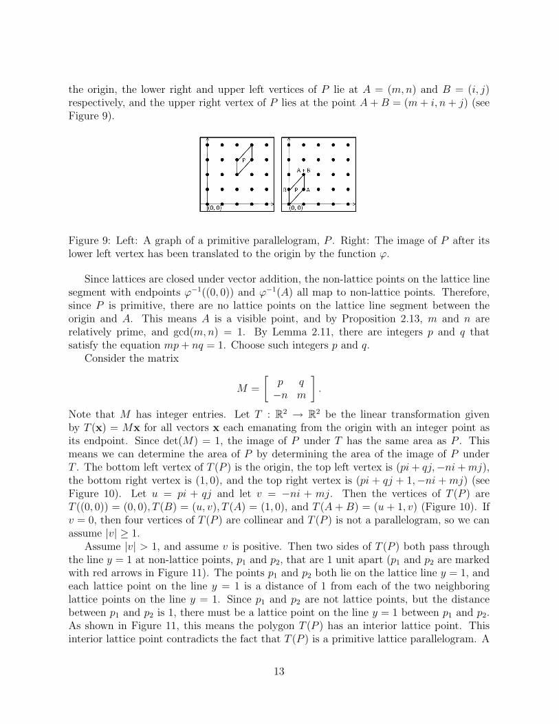
the origin, the lower right and upper left vertices of P lie at A = (m, n) and B = (i, j)respectively, and the upper right vertex of P lies at the point A + B = (m + i, n + j) (seeFigure 9).

Figure 9: Left: A graph of a primitive parallelogram, P . Right: The image of P after itslower left vertex has been translated to the origin by the function ϕ.

Since lattices are closed under vector addition, the non-lattice points on the lattice linesegment with endpoints ϕ−1((0, 0)) and ϕ−1(A) all map to non-lattice points. Therefore,since P is primitive, there are no lattice points on the lattice line segment between theorigin and A. This means A is a visible point, and by Proposition 2.13, m and n arerelatively prime, and gcd(m, n) = 1. By Lemma 2.11, there are integers p and q thatsatisfy the equation mp + nq = 1. Choose such integers p and q.

Consider the matrix

M =

[p q−n m

].

Note that M has integer entries. Let T : R2 → R2 be the linear transformation givenby T (x) = Mx for all vectors x each emanating from the origin with an integer point asits endpoint. Since det(M) = 1, the image of P under T has the same area as P . Thismeans we can determine the area of P by determining the area of the image of P underT . The bottom left vertex of T (P ) is the origin, the top left vertex is (pi + qj,−ni + mj),the bottom right vertex is (1, 0), and the top right vertex is (pi + qj + 1,−ni + mj) (seeFigure 10). Let u = pi + qj and let v = −ni + mj. Then the vertices of T (P ) areT ((0, 0)) = (0, 0), T (B) = (u, v), T (A) = (1, 0), and T (A + B) = (u + 1, v) (Figure 10). Ifv = 0, then four vertices of T (P ) are collinear and T (P ) is not a parallelogram, so we canassume |v| ≥ 1.

Assume |v| > 1, and assume v is positive. Then two sides of T (P ) both pass throughthe line y = 1 at non-lattice points, p1 and p2, that are 1 unit apart (p1 and p2 are markedwith red arrows in Figure 11). The points p1 and p2 both lie on the lattice line y = 1, andeach lattice point on the line y = 1 is a distance of 1 from each of the two neighboringlattice points on the line y = 1. Since p1 and p2 are not lattice points, but the distancebetween p1 and p2 is 1, there must be a lattice point on the line y = 1 between p1 and p2.As shown in Figure 11, this means the polygon T (P ) has an interior lattice point. Thisinterior lattice point contradicts the fact that T (P ) is a primitive lattice parallelogram. A

13

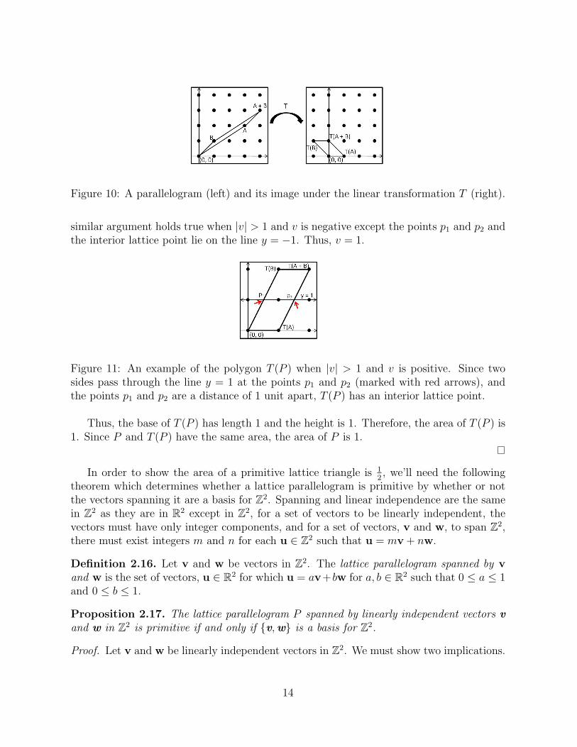
Figure 10: A parallelogram (left) and its image under the linear transformation T (right).

similar argument holds true when |v| > 1 and v is negative except the points p1 and p2 andthe interior lattice point lie on the line y = −1. Thus, v = 1.

Figure 11: An example of the polygon T (P ) when |v| > 1 and v is positive. Since twosides pass through the line y = 1 at the points p1 and p2 (marked with red arrows), andthe points p1 and p2 are a distance of 1 unit apart, T (P ) has an interior lattice point.

Thus, the base of T (P ) has length 1 and the height is 1. Therefore, the area of T (P ) is1. Since P and T (P ) have the same area, the area of P is 1.

In order to show the area of a primitive lattice triangle is 12, we’ll need the following

theorem which determines whether a lattice parallelogram is primitive by whether or notthe vectors spanning it are a basis for Z2. Spanning and linear independence are the samein Z2 as they are in R2 except in Z2, for a set of vectors to be linearly independent, thevectors must have only integer components, and for a set of vectors, v and w, to span Z2,there must exist integers m and n for each u ∈ Z2 such that u = mv + nw.

Definition 2.16. Let v and w be vectors in Z2. The lattice parallelogram spanned by vand w is the set of vectors, u ∈ R2 for which u = av+bw for a, b ∈ R2 such that 0 ≤ a ≤ 1and 0 ≤ b ≤ 1.

Proposition 2.17. The lattice parallelogram P spanned by linearly independent vectors vand w in Z2 is primitive if and only if {v,w} is a basis for Z2.

Proof. Let v and w be linearly independent vectors in Z2. We must show two implications.

14

(=⇒) Let P be the primitive parallelogram spanned by v and w. Since v and w are linearlyindependent, they form a basis for R2 over R. Let u ∈ Z2. Then u can be writtenas a linear combination of v and w. Choose a, b ∈ R such that u = av + bw. Weshow v and w span Z2 by showing that a and b must be integers. Let a = bac + a′,let b = bbc + b′, and note that 0 ≤ a′ < 1 and 0 ≤ b′ < 1. Let u0 ∈ R2 andlet u0 = a′v + b′w. Then u0 = u − bacv − bbcw. Since u,v, and w ∈ Z2 andbac, bbc ∈ Z, u0 ∈ Z2. We know a′ < 1, b′ < 1, and v and w span P . Therefore, u0 isin P . However, P is primitive, so u0 must be a vertex of P . Since a′ 6= 1 and b′ 6= 1,u0 = (0, 0). It follows that a′ = b′ = 0 since u0 = a′v + b′w, v 6= 0, and u 6= 0. Thismeans a and b are integers, and therefore, v and w span Z2. Thus, since v and ware linearly independent, {v,w} is a basis for Z2.

(⇐=) Let {v,w} be a basis for Z2. Then for any vector u ∈ Z2, u = mv + nw for someintegers m and n. Let P be the parallelogram spanned by v and w. Assume u ∈ Z2

is in P . We must show u is a vertex of P . Since P is spanned by v and w, we canwrite u = av + bw where a, b ∈ R, 0 ≤ a ≤ 1, and 0 ≤ b ≤ 1. This means m and nmust each be 0 or 1. Thus, u is a vertex of P , and P is primitive.

2.6 The Area of a Primitive Lattice Triangle

Now, we use the facts about plane isometry and visible points, together with our resultsabout primitive parallelograms to prove the area of a primitive lattice triangle is 1

2. We’ll

need to know the sides of a primitive lattice triangle form a bas is of Z2. The followinglemma shows this is the case.

Lemma 2.18. If the vectors v and w correspond to adjacent sides of a primitive latticetriangle T , then v and w form a basis of Z2.

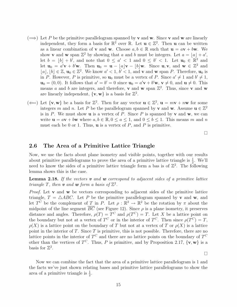
Proof. Let v and w be vectors corresponding to adjacent sides of the primitive latticetriangle, T = 4ABC. Let P be the primitive parallelogram spanned by v and w, andlet TC be the complement of T in P . Let ρ : R2 → R2 be the rotation by π about themidpoint of the line segment BC (see Figure 12). Since ρ is a plane isometry, it preservesdistance and angles. Therefore, ρ(T ) = TC and ρ(TC) = T . Let X be a lattice point onthe boundary but not at a vertex of TC or in the interior of TC . Then since ρ(TC) = T ,ρ(X) is a lattice point on the boundary of T but not at a vertex of T or ρ(X) is a latticepoint in the interior of T . Since T is primitive, this is not possible. Therefore, there are nolattice points in the interior of TC and there are no lattice points on the boundary of TC

other than the vertices of TC . Thus, P is primitive, and by Proposition 2.17, {v,w} is abasis for Z2.

Now we can combine the fact that the area of a primitive lattice parallelogram is 1 andthe facts we’ve just shown relating bases and primitive lattice parallelograms to show thearea of a primitive triangle is 1

2.

15

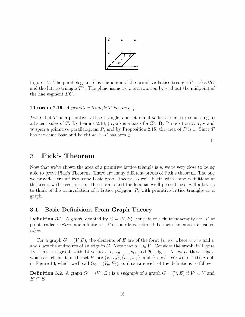
Figure 12: The parallelogram P is the union of the primitive lattice triangle T = 4ABCand the lattice triangle TC . The plane isometry ρ is a rotation by π about the midpoint ofthe line segment BC.

Theorem 2.19. A primitive triangle T has area 12.

Proof. Let T be a primitive lattice triangle, and let v and w be vectors corresponding toadjacent sides of T . By Lemma 2.18, {v,w} is a basis for Z2. By Proposition 2.17, v andw span a primitive parallelogram P , and by Proposition 2.15, the area of P is 1. Since Thas the same base and height as P , T has area 1

2.

3 Pick’s Theorem

Now that we’ve shown the area of a primitive lattice triangle is 12, we’re very close to being

able to prove Pick’s Theorem. There are many different proofs of Pick’s theorem. The onewe provide here utilizes some basic graph theory, so we’ll begin with some definitions ofthe terms we’ll need to use. These terms and the lemmas we’ll present next will allow usto think of the triangulation of a lattice polygon, P , with primitive lattice triangles as agraph.

3.1 Basic Definitions From Graph Theory

Definition 3.1. A graph, denoted by G = (V, E), consists of a finite nonempty set, V ofpoints called vertices and a finite set, E of unordered pairs of distinct elements of V , callededges.

For a graph G = (V, E), the elements of E are of the form {u, v}, where u 6= v and uand v are the endpoints of an edge in G. Note that u, v ∈ V . Consider the graph, in Figure13. This is a graph with 14 vertices, v1, v2, . . . , v14 and 20 edges. A few of these edges,which are elements of the set E, are {v1, v2}, {v11, v12}, and {v8, v9}. We will use the graphin Figure 13, which we’ll call G0 = (V0, E0), to illustrate each of the definitions to follow.

Definition 3.2. A graph G′ = (V ′, E ′) is a subgraph of a graph G = (V, E) if V ′ ⊆ V andE ′ ⊆ E.

16

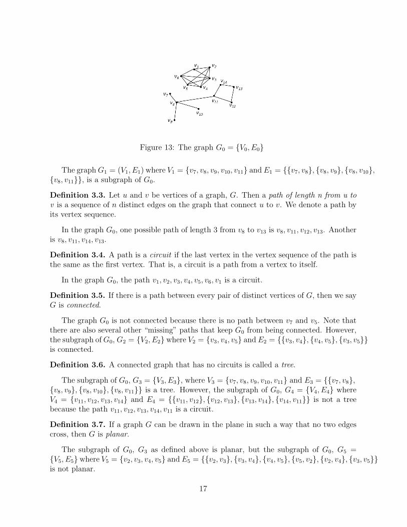
Figure 13: The graph G0 = {V0, E0}

The graph G1 = (V1, E1) where V1 = {v7, v8, v9, v10, v11} and E1 = {{v7, v8}, {v8, v9}, {v8, v10},{v8, v11}}, is a subgraph of G0.

Definition 3.3. Let u and v be vertices of a graph, G. Then a path of length n from u tov is a sequence of n distinct edges on the graph that connect u to v. We denote a path byits vertex sequence.

In the graph G0, one possible path of length 3 from v8 to v13 is v8, v11, v12, v13. Anotheris v8, v11, v14, v13.

Definition 3.4. A path is a circuit if the last vertex in the vertex sequence of the path isthe same as the first vertex. That is, a circuit is a path from a vertex to itself.

In the graph G0, the path v1, v2, v3, v4, v5, v6, v1 is a circuit.

Definition 3.5. If there is a path between every pair of distinct vertices of G, then we sayG is connected.

The graph G0 is not connected because there is no path between v7 and v5. Note thatthere are also several other “missing” paths that keep G0 from being connected. However,the subgraph of G0, G2 = {V2, E2} where V2 = {v3, v4, v5} and E2 = {{v3, v4}, {v4, v5}, {v3, v5}}is connected.

Definition 3.6. A connected graph that has no circuits is called a tree.

The subgraph of G0, G3 = {V3, E3}, where V3 = {v7, v8, v9, v10, v11} and E3 = {{v7, v8},{v8, v9}, {v8, v10}, {v8, v11}} is a tree. However, the subgraph of G0, G4 = {V4, E4} whereV4 = {v11, v12, v13, v14} and E4 = {{v11, v12}, {v12, v13}, {v13, v14}, {v14, v11}} is not a treebecause the path v11, v12, v13, v14, v11 is a circuit.

Definition 3.7. If a graph G can be drawn in the plane in such a way that no two edgescross, then G is planar.

The subgraph of G0, G3 as defined above is planar, but the subgraph of G0, G5 ={V5, E5} where V5 = {v2, v3, v4, v5} and E5 = {{v2, v3}, {v3, v4}, {v4, v5}, {v5, v2}, {v2, v4}, {v3, v5}}is not planar.

17

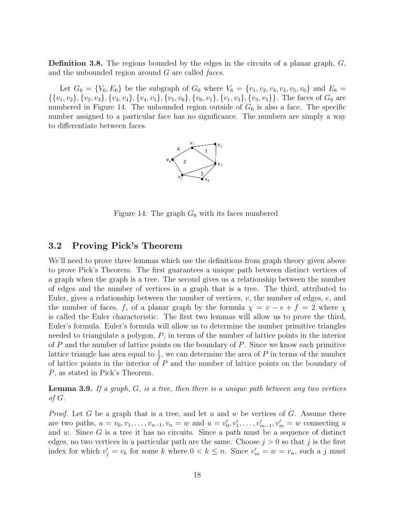
Definition 3.8. The regions bounded by the edges in the circuits of a planar graph, G,and the unbounded region around G are called faces.

Let G6 = {V6, E6} be the subgraph of G0 where V6 = {v1, v2, v3, v4, v5, v6} and E6 ={{v1, v2}, {v2, v3}, {v3, v4}, {v4, v5}, {v5, v6}, {v6, v1}, {v1, v3}, {v3, v5}}. The faces of G6 arenumbered in Figure 14. The unbounded region outside of G6 is also a face. The specificnumber assigned to a particular face has no significance. The numbers are simply a wayto differentiate between faces.

Figure 14: The graph G6 with its faces numbered

3.2 Proving Pick’s Theorem

We’ll need to prove three lemmas which use the definitions from graph theory given aboveto prove Pick’s Theorem. The first guarantees a unique path between distinct vertices ofa graph when the graph is a tree. The second gives us a relationship between the numberof edges and the number of vertices in a graph that is a tree. The third, attributed toEuler, gives a relationship between the number of vertices, v, the number of edges, e, andthe number of faces, f , of a planar graph by the formula χ = v − e + f = 2 where χis called the Euler characteristic. The first two lemmas will allow us to prove the third,Euler’s formula. Euler’s formula will allow us to determine the number primitive trianglesneeded to triangulate a polygon, P , in terms of the number of lattice points in the interiorof P and the number of lattice points on the boundary of P . Since we know each primitivelattice triangle has area equal to 1

2, we can determine the area of P in terms of the number

of lattice points in the interior of P and the number of lattice points on the boundary ofP , as stated in Pick’s Theorem.

Lemma 3.9. If a graph, G, is a tree, then there is a unique path between any two verticesof G.

Proof. Let G be a graph that is a tree, and let u and w be vertices of G. Assume thereare two paths, u = v0, v1, . . . , vn−1, vn = w and u = v′0, v

′1, . . . , v

′m−1, v

′m = w connecting u

and w. Since G is a tree it has no circuits. Since a path must be a sequence of distinctedges, no two vertices in a particular path are the same. Choose j > 0 so that j is the firstindex for which v′j = vk for some k where 0 < k ≤ n. Since v′m = w = vn, such a j must

18

exist. The path u, v1, v2, . . . , vk, v′j−1, . . . , v

′2, v

′1, u is a circuit in G. Since G is a tree, this is

a contradiction. Thus, there is a unique path between any two vertices in G.

Lemma 3.10. If a graph, G, is a tree with v vertices and e edges, then e = v − 1.

Proof. Let G = {V, E} be a graph that is a tree, and let u be a vertex in G. By Lemma3.9, for each vertex, w ∈ V \ {u}, there is a unique path from u to w. For each vertexw ∈ V \ {u}, associate the last edge in the unique path from u to w with w. Note thatevery edge in G is the last edge in the unique path from u to w for some vertex w ∈ V \{u}.Since G is a tree, there is a one to one correspondence between V \{u} and E. This meansthat V \ {u} and E have the same number of elements. Thus, e = v − 1.

Lemma 3.11. (Euler) If G is a connected, planar graph with v vertices, e edges, and ffaces, then v − e + f = 2.

Proof. Let G be a connected, planar graph with v vertices, e edges, and f faces. Weproceed by induction on e. For the base case, let e = 0. Since G is connected, v = 1 andf = 1. Thus, v − e + f = 1− 0 + 1 = 2.

Let e > 0 and assume Euler’s formula holds for all connected planar graphs with e− 1edges. We must show v − e + f = 2.

Assume G does not contain a circuit. Then G is a tree. Thus, f = 1, and by Lemma3.10, e = v − 1. Thus, v − e + f = v − (v − 1) + 1 = v − v + 1 + 1 = 2.

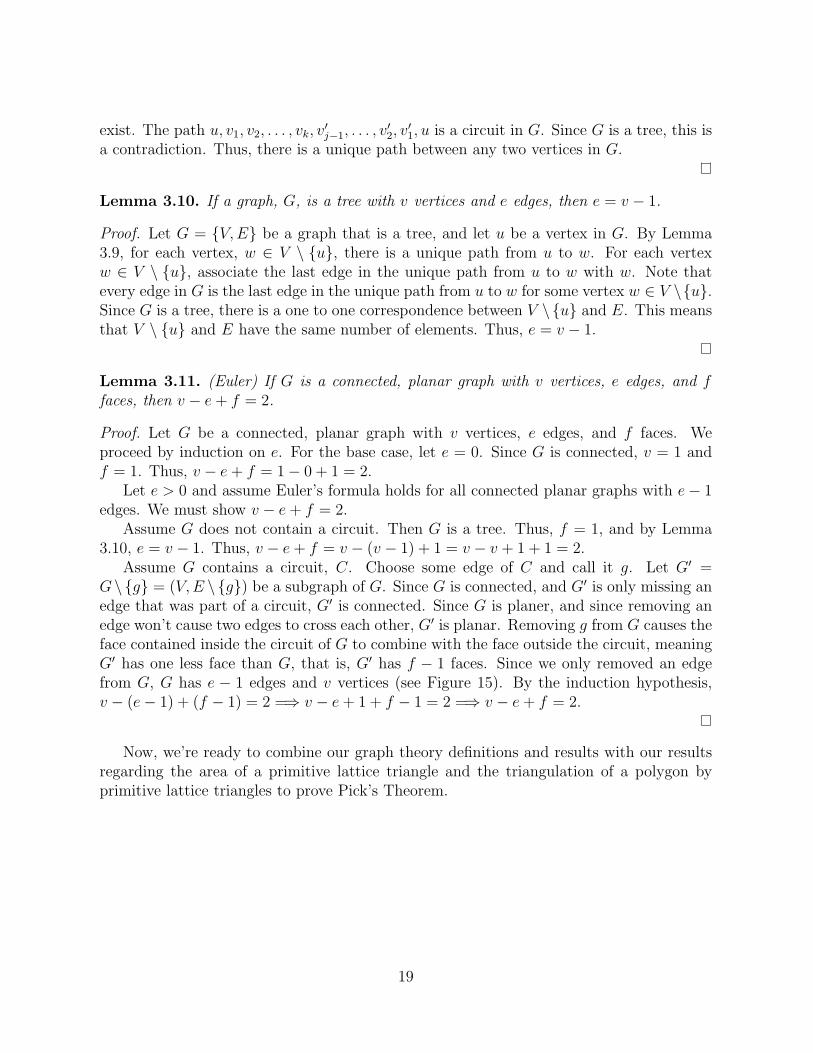
Assume G contains a circuit, C. Choose some edge of C and call it g. Let G′ =G \ {g} = (V, E \ {g}) be a subgraph of G. Since G is connected, and G′ is only missing anedge that was part of a circuit, G′ is connected. Since G is planer, and since removing anedge won’t cause two edges to cross each other, G′ is planar. Removing g from G causes theface contained inside the circuit of G to combine with the face outside the circuit, meaningG′ has one less face than G, that is, G′ has f − 1 faces. Since we only removed an edgefrom G, G has e − 1 edges and v vertices (see Figure 15). By the induction hypothesis,v − (e− 1) + (f − 1) = 2 =⇒ v − e + 1 + f − 1 = 2 =⇒ v − e + f = 2.

Now, we’re ready to combine our graph theory definitions and results with our resultsregarding the area of a primitive lattice triangle and the triangulation of a polygon byprimitive lattice triangles to prove Pick’s Theorem.

19

Figure 15: Left: The connected, planar, graph G7 which is a subgraph of the graph G0

shown in Figure 13. The faces of G7 are numbered. We will remove the edge {v12, v13}which is indicated by the arrow to obtain the subgraph of G7, G′

7. Right: The graph G′7

is connected and planar, and G′7 has one fewer region and one fewer edge, but the same

number of vertices as G7.

Theorem 3.12 (Pick’s Theorem). Let P be a polygon in the plane with its vertices atlattice points. Then the area of P , A(P ), is given by

A(P ) =1

2B(P ) + I(P )− 1.

where B(P ) is the number of lattice points on the boundary of P and I(P ) is the numberof lattice points in the interior of P .

Proof. Let P be a lattice polygon with B(P ) lattice points on its boundary and I(P ) latticepoints in its interior. By Theorem 2.8, we can dissect P into primitive lattice triangles.Note that the sides of the triangles do not intersect and since the triangles are primitive,each lattice point in P is a vertex of a triangle. This means the graph, G, whose verticesare the lattice points in P and whose edges are the sides of the primitive triangles thattriangulate P is planar and connected.

Let f be the number of faces in G, let e be the number of edges in G, and let v be thenumber of vertices in G. Then there are f − 1 primitive triangles in P . The other face inG is the unbounded space outside P . By Theorem 2.19, the area of a primitive triangle is12, so, since P contains f − 1 primitive triangles,

A(P ) =1

2(f − 1). (1)

Now let’s consider the number of edges in G. Each of the ei edges in G living insidethe polygon P is shared as a side of two primitive lattice triangles. Each of the eb edgesliving on the boundary of the polygon P is a side of one primitive triangle. Since theedges in G are the lattice line segments that form the sides of the primitive triangles in P ,ei + eb = e =⇒ ei = e− eb.

Since f − 1 primitive triangles triangulate P , the number of sides of primitive trianglesin P is given as follows,

20

3(f − 1) = 2ei + eb = 2(e− eb) + eb = 2e− 2eb + eb = 2e− eb.

Solving for f gives,

f = 2(e− f)− eb + 3. (2)

By Lemma 3.11, v − e + f = 2 =⇒ e = v + f − 2. Substituting this into equation (2), weget

f = 2(v − 2)− eb + 3. (3)

Since we can associate each of the eb edges of G lying on the boundary of P with one latticepoint on the boundary of P , and this accounts for all lattice points on the boundary of P ,there are eb lattice points on the boundary of P , so B(P ) = eb. As mentioned above, thevertices of G are the interior and boundary lattice points of P . Therefore, v = B(P )+I(P ).Substituting this, eb = B(P ), and equation (3) into equation (1) gives

A(P ) =1

2(f − 1)

=1

2(2(v − 2)− eb + 2)

=1

2(2((B(P ) + I(P ))− 2)−B(P ) + 2)

=1

2B(P ) + I(P )− 1.

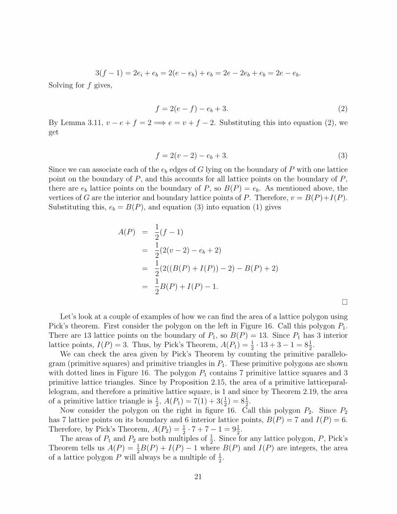
Let’s look at a couple of examples of how we can find the area of a lattice polygon usingPick’s theorem. First consider the polygon on the left in Figure 16. Call this polygon P1.There are 13 lattice points on the boundary of P1, so B(P ) = 13. Since P1 has 3 interiorlattice points, I(P ) = 3. Thus, by Pick’s Theorem, A(P1) = 1

2· 13 + 3− 1 = 81

2.

We can check the area given by Pick’s Theorem by counting the primitive parallelo-gram (primitive squares) and primitive triangles in P1. These primitive polygons are shownwith dotted lines in Figure 16. The polygon P1 contains 7 primitive lattice squares and 3primitive lattice triangles. Since by Proposition 2.15, the area of a primitive latticeparal-lelogram, and therefore a primitive lattice square, is 1 and since by Theorem 2.19, the areaof a primitive lattice triangle is 1

2, A(P1) = 7(1) + 3(1

2) = 81

2.

Now consider the polygon on the right in figure 16. Call this polygon P2. Since P2

has 7 lattice points on its boundary and 6 interior lattice points, B(P ) = 7 and I(P ) = 6.Therefore, by Pick’s Theorem, A(P2) = 1

2· 7 + 7− 1 = 91

2.

The areas of P1 and P2 are both multiples of 12. Since for any lattice polygon, P , Pick’s

Theorem tells us A(P ) = 12B(P ) + I(P ) − 1 where B(P ) and I(P ) are integers, the area

of a lattice polygon P will always be a multiple of 12.

21

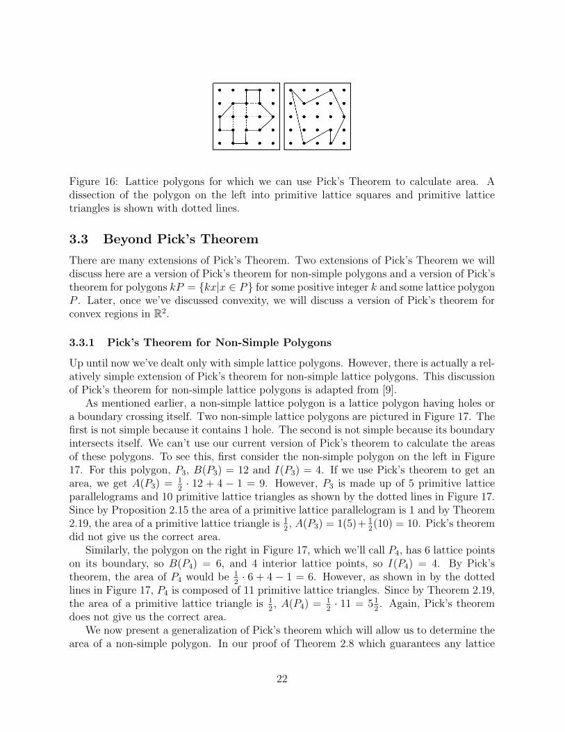
Figure 16: Lattice polygons for which we can use Pick’s Theorem to calculate area. Adissection of the polygon on the left into primitive lattice squares and primitive latticetriangles is shown with dotted lines.

3.3 Beyond Pick’s Theorem

There are many extensions of Pick’s Theorem. Two extensions of Pick’s Theorem we willdiscuss here are a version of Pick’s theorem for non-simple polygons and a version of Pick’stheorem for polygons kP = {kx|x ∈ P} for some positive integer k and some lattice polygonP . Later, once we’ve discussed convexity, we will discuss a version of Pick’s theorem forconvex regions in R2.

3.3.1 Pick’s Theorem for Non-Simple Polygons

Up until now we’ve dealt only with simple lattice polygons. However, there is actually a rel-atively simple extension of Pick’s theorem for non-simple lattice polygons. This discussionof Pick’s theorem for non-simple lattice polygons is adapted from [9].

As mentioned earlier, a non-simple lattice polygon is a lattice polygon having holes ora boundary crossing itself. Two non-simple lattice polygons are pictured in Figure 17. Thefirst is not simple because it contains 1 hole. The second is not simple because its boundaryintersects itself. We can’t use our current version of Pick’s theorem to calculate the areasof these polygons. To see this, first consider the non-simple polygon on the left in Figure17. For this polygon, P3, B(P3) = 12 and I(P3) = 4. If we use Pick’s theorem to get anarea, we get A(P3) = 1

2· 12 + 4 − 1 = 9. However, P3 is made up of 5 primitive lattice

parallelograms and 10 primitive lattice triangles as shown by the dotted lines in Figure 17.Since by Proposition 2.15 the area of a primitive lattice parallelogram is 1 and by Theorem2.19, the area of a primitive lattice triangle is 1

2, A(P3) = 1(5)+ 1

2(10) = 10. Pick’s theorem

did not give us the correct area.Similarly, the polygon on the right in Figure 17, which we’ll call P4, has 6 lattice points

on its boundary, so B(P4) = 6, and 4 interior lattice points, so I(P4) = 4. By Pick’stheorem, the area of P4 would be 1

2· 6 + 4 − 1 = 6. However, as shown in by the dotted

lines in Figure 17, P4 is composed of 11 primitive lattice triangles. Since by Theorem 2.19,the area of a primitive lattice triangle is 1

2, A(P4) = 1

2· 11 = 51

2. Again, Pick’s theorem

does not give us the correct area.We now present a generalization of Pick’s theorem which will allow us to determine the

area of a non-simple polygon. In our proof of Theorem 2.8 which guarantees any lattice

22

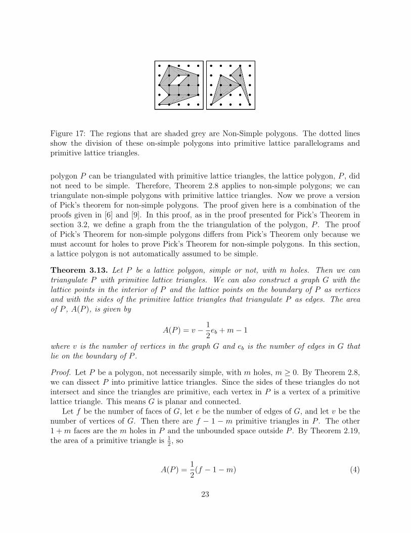
Figure 17: The regions that are shaded grey are Non-Simple polygons. The dotted linesshow the division of these on-simple polygons into primitive lattice parallelograms andprimitive lattice triangles.

polygon P can be triangulated with primitive lattice triangles, the lattice polygon, P , didnot need to be simple. Therefore, Theorem 2.8 applies to non-simple polygons; we cantriangulate non-simple polygons with primitive lattice triangles. Now we prove a versionof Pick’s theorem for non-simple polygons. The proof given here is a combination of theproofs given in [6] and [9]. In this proof, as in the proof presented for Pick’s Theorem insection 3.2, we define a graph from the the triangulation of the polygon, P . The proofof Pick’s Theorem for non-simple polygons differs from Pick’s Theorem only because wemust account for holes to prove Pick’s Theorem for non-simple polygons. In this section,a lattice polygon is not automatically assumed to be simple.

Theorem 3.13. Let P be a lattice polygon, simple or not, with m holes. Then we cantriangulate P with primitive lattice triangles. We can also construct a graph G with thelattice points in the interior of P and the lattice points on the boundary of P as verticesand with the sides of the primitive lattice triangles that triangulate P as edges. The areaof P , A(P ), is given by

A(P ) = v − 1

2eb + m− 1

where v is the number of vertices in the graph G and eb is the number of edges in G thatlie on the boundary of P .

Proof. Let P be a polygon, not necessarily simple, with m holes, m ≥ 0. By Theorem 2.8,we can dissect P into primitive lattice triangles. Since the sides of these triangles do notintersect and since the triangles are primitive, each vertex in P is a vertex of a primitivelattice triangle. This means G is planar and connected.

Let f be the number of faces of G, let e be the number of edges of G, and let v be thenumber of vertices of G. Then there are f − 1 − m primitive triangles in P . The other1 + m faces are the m holes in P and the unbounded space outside P . By Theorem 2.19,the area of a primitive triangle is 1

2, so

A(P ) =1

2(f − 1−m) (4)

23

As in our proof of Pick’s theorem, ei + eb = e =⇒ ei = e− eb where e is the total numberof edges in G, ei is the number of edges in G that lie in the interior of P , and eb is thenumber of edges in G that lie on the boundary of P . Since f − 1 −m primitive trianglestriangulate P ,

3(f − 1−m) = 2ei + eb = 2e− eb. (5)

Solving for f yields

f = 2(e− f)− eb + 3(m + 1). (6)

Since G is connected and planar, by Lemma 3.11, v − e + f = 2 =⇒ e = v + f − 2.Substituting this into equation (6), we get

f = 2(v − 2)− eb + 3(m + 1). (7)

Finally, substituting equation (7) into equation (4) gives us

A(P ) = v − 1

2eb + m− 1. (8)

With this extension of Pick’s theorem, we can now find the areas of the non-simplepolygons in Figure 3.13 without dissecting the polygons into primitive lattice triangles andprimitive lattice parallelograms. The polygon P3 has 16 lattice points on its boundary andin its interior, so v = 16, 12 edges on its boundary, so eb = 12, and 1 hole, so m = 1.Therefore, by Theorem 3.13, A(P3) = 16− 1

2· 12 + 1− 1 = 10, which is the correct area.

The polygon P4 has 10 lattice points on its boundary and in its interior, so v = 10,7 edges on its boundary, so eb = 7, and 0 holes, so m = 0. Thus, by Theorem 3.13,A(P4) = 10− 1

2· 7 + 0− 1 = 51

2. Once again, the area given by our generalization of Pick’s

theorem is the same as the area given by dissecting P4 into primitive polygons.Note that we did not express the area of P in terms of B(P ) and I(P ) for the version

of Pick’s theorem for non-simple polygons like we did for Pick’s theorem. This is becausefor some non-simple polygons, the equation eb = B(P ) is not true. For example, considerthe non-simple polygon, P5 in Figure 18. The polygon P5 has 14 edges on its boundary,but it has 13 lattice points on its boundary, so eb = 14 6= 13 = B(P5).

The area of a simple polygon, P , as given by Pick’s theorem is A(P ) = 12B(P )+I(P )−1.

However, if we don’t set eb = B(P ) and v = B(P ) + I(P ), then the area given by Pick’stheorem is v− 1

2eb− 1. From this, we see the only differences between the version of Pick’s

theorem for non-simple polygons and Pick’s theorem are first, for a non-simple polygon,we cannot write the area in terms of the numbers of boundary and interior lattice pointsin P and second, for the generalization of Pick’s theorem to non-simple polygons, we mustfactor in the number of holes in P .

24

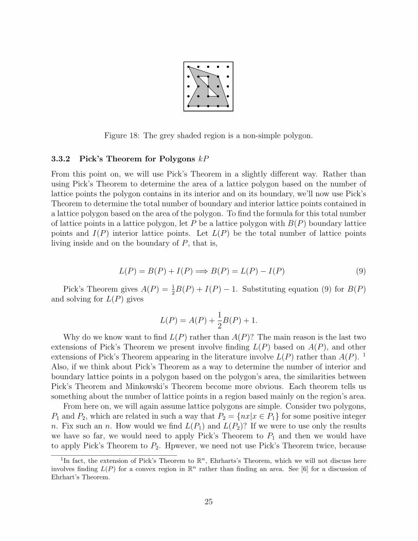
Figure 18: The grey shaded region is a non-simple polygon.

3.3.2 Pick’s Theorem for Polygons kP

From this point on, we will use Pick’s Theorem in a slightly different way. Rather thanusing Pick’s Theorem to determine the area of a lattice polygon based on the number oflattice points the polygon contains in its interior and on its boundary, we’ll now use Pick’sTheorem to determine the total number of boundary and interior lattice points contained ina lattice polygon based on the area of the polygon. To find the formula for this total numberof lattice points in a lattice polygon, let P be a lattice polygon with B(P ) boundary latticepoints and I(P ) interior lattice points. Let L(P ) be the total number of lattice pointsliving inside and on the boundary of P , that is,

L(P ) = B(P ) + I(P ) =⇒ B(P ) = L(P )− I(P ) (9)

Pick’s Theorem gives A(P ) = 12B(P ) + I(P ) − 1. Substituting equation (9) for B(P )

and solving for L(P ) gives

L(P ) = A(P ) +1

2B(P ) + 1.

Why do we know want to find L(P ) rather than A(P )? The main reason is the last twoextensions of Pick’s Theorem we present involve finding L(P ) based on A(P ), and otherextensions of Pick’s Theorem appearing in the literature involve L(P ) rather than A(P ). 1

Also, if we think about Pick’s Theorem as a way to determine the number of interior andboundary lattice points in a polygon based on the polygon’s area, the similarities betweenPick’s Theorem and Minkowski’s Theorem become more obvious. Each theorem tells ussomething about the number of lattice points in a region based mainly on the region’s area.

From here on, we will again assume lattice polygons are simple. Consider two polygons,P1 and P2, which are related in such a way that P2 = {nx|x ∈ P1} for some positive integern. Fix such an n. How would we find L(P1) and L(P2)? If we were to use only the resultswe have so far, we would need to apply Pick’s Theorem to P1 and then we would haveto apply Pick’s Theorem to P2. Hpwever, we need not use Pick’s Theorem twice, because

1In fact, the extension of Pick’s Theorem to Rn, Ehrharts’s Theorem, which we will not discuss hereinvolves finding L(P ) for a convex region in Rn rather than finding an area. See [6] for a discussion ofEhrhart’s Theorem.

25

there is an extension of Pick’s Theorem that gives a formula for L(kP ), where P is a latticepolygon, and kP = {kx|x ∈ P} for any positive integer k. We’ll call This formula Pick’sTheorem for polygons kP . To prove it, we’ll need a few lemmas.

The first two lemmas require a return to visible points. We will determine the coordi-nates of lattice points on a line l in terms of the visible points on l and we will use thisresult to determine the number of lattice points on a line between a lattice point and theorigin. Since we can translate any lattice polygon so one of its vertices lies at the originwhile ensuring lattice points remain lattice points and non-lattice points remain non-latticepoint, the edges of the polygon adjacent to the vertex that is mapped to the origin be-come lattice line segments from a lattice point to the origin. The results we’ve mentionedhere and we’ll prove next, will allow us to determine the number of lattice points on theboundary of a polygon based on the number of lattice points on each edge of the polygon.

Recall that a visible point is the point on a particular line through the origin lyingclosest to the origin.

Lemma 3.14. If p = (m, n) is a visible point on the lattice line l, then the lattice pointson l are each of the form tp for some integer t.

Proof. Let p = (j, k) be a visible point on the lattice line l. Let q = (m,n) be a latticepoint on l that is distinct from p. Since l passes through q = (m, n) and (0, 0), the equationfor l is y = n

mx. Since q is not visible, by Theorem 2.13, m and n are not relatively prime,

that is, gcd(m, n) = d > 1 for some integer d. It follows that md

and nd

are integers and(m

d, n

d) is therefore a lattice point. Since the point (m

d, n

d) satisfies y = n

mx, (m

d, n

d) is on l.

Since d = gcd(m,n), gcd(md, n

d) = 1. Therefore, by Theorem 2.13, (m

d, n

d) is visible. This

means (md, n

d) = ±p. Thus, q = ±dp.

Lemma 3.15. Let m and n be nonnegative integers. There are exactly gcd(m, n)−1 latticepoints on the lattice line segment between the origin and the point (m, n) not including theendpoints.

Proof. Let (m, n) be a lattice point, and let l be the lattice line segment with endpoints(0, 0) and (m,n). Let gcd(m, n) = d. Then gcd(m

d, n

d) = 1, and by Theorem 2.13, (m

d, n

d)

is visible. By Lemma 3.14, the lattice points on l other than (0, 0) and (m, n) must be

(md, n

d), (2m

d, 2n

d), (3m

d, 3n

d), . . . , ( (d−1)m

d, (d−1)n

d). Thus, there are d−1 points on l not including

its endpoints.

In the following lemma, we’ll use the results we just proved about visible points to givea formula for the number of points on the boundary of a lattice polygon P .

Lemma 3.16. Let P be a lattice n-gon with vertices p1 = (a1, b1), p2 = (a2, b2), . . . , pn =(an, bn). If di = gcd(ai+1 − ai, bi+1 − bi), then the number of lattice points on the boundaryof P , B(P ), is

26

B(P ) =n∑

i=1

di.

Proof. Let P be a lattice n-gon with vertices p1 = (a1, b1), p2 = (a2, b2), . . . , pn = (an, bn).Let gcd(ai+1−ai, bi+1−bi) = di, 1 ≤ i < n and let gcd(a1−ai, b1−bi) = di when i = n. Sincetranslation is a plane isometry, and a lattice must be closed under vector addition, distanceand the number of lattice points on a lattice line are preserved under translation. Therefore,we can translate each side of P with endpoints pi and pi+1 by a lattice point, pi, so oneof its endpoints, pi = (ai, bi) lies at the origin. After this translation, the other endpoint,pi+1 = (ai+1, bi+1) lies at the point (ai+1−ai, bi+1−bi). Note that we can map the side withendpoints pn and p1 to the line segment with endpoints at the origin and (a1− an, b1− bn).Since gcd(ai+1−ai, bi+1−bi) = di when 1 ≤ i < n and gcd(a1−an, b1−bn) = di, by Lemma3.15, there are di − 1 lattice points on the side of P with endpoints pi and pi+1 (or withendpoints pn and p1) not including pi and pi+1 (or pn and p1). Since di−1 gives the numberof lattice points on the side of P with pi and pi+1 as endpoints for every i < n, and di − 1gives the number of lattice points on the side of P with pn and p1 as endpoints for i = n,we know the number of lattice points that are not vertices on each side of P . Therefore,the number of lattice points on the boundary of P not counting the vertices of P , is

n∑i=1

(di − 1).

Thus, adding in the vertices of P gives

B(P ) = n +n∑

i=1

(di − 1)

= n + (d1 − 1) + (d2 − 1) + · · ·+ (dn − 1)

= n + d1 + d2 + · · ·+ dn − n

= d1 + d2 + · · ·+ dn

=n∑

i=1

di.

The last thing we need in order to prove our generalization of Pick’s theorem for poly-gons kP is the fact that multiplication of every point in a polygon by some integer k changesthe lengths of the sides of the polygon by a factor of k and changes the area of the polygonby a factor of k2. This can be shown with some simple linear algebra. Let M : R2 → R2

be the linear transformation given by Mx = kx where x is a vector in R2 emanating fromthe origin with its endpoint at a lattice point and M is the matrix

27

M =

[k 00 k

].

Under M , the vector v = 〈x, y〉 is mapped to the vector kv = 〈kx, ky〉 = k〈x, y〉 so thelength of the vector v is changed by a factor of k. Since det(M) = k2, the area of the imageunder M of any closed, bounded region, R, in R2 is different from the area of R by a factorof k2. Now we can find a formula for the number of lattice points in a polygon kP . Notethat the are of R will still change by a factor of k2 even if k is a positive real number that isnot an integer. We assume k is an integer here, becasue we will need this condition in thenext theorem so we can talk about the greatest common divisor of an integer multiplied byk. However, we will need to consider changes in area when k is not an integer later whenwe prove Minkowski’s Theorem.

Theorem 3.17. Let P be a polygon, let k be a positive integer, and define kP = {kx|x ∈P}. Then the number of boundary and interior lattice points in kP , L(kP ), is

L(kP ) = A(P )k2 +1

2B(P )k + 1

where B(P ) and A(P ) are defined as for Pick’s Theorem.

Proof. Let P be an n-gon, let k be a positive integer, and define kP = {kx|x ∈ P}.Equation (??) gives us

L(kP ) = A(kP ) +1

2B(kP ) + 1.

Lemma 3.16 and the fact that gcd(ka, kb) = k gcd(a, b) give us that

B(kP ) =n∑

i=1

di

=n∑

i=1

gcd(k(ai+1 − ai), k(bi+1 − bi))

= k

n∑i=1

gcd(ai+1 − ai, bi+1 − bi)

= B(P )k.

As we discussed above, multiplication of every point in P by k changes the area of P by afactor of k2, so A(kP ) = A(P )k2. Thus,

L(kP ) = A(P )k2 +1

2B(P )k + 1.

28

This generalization of Pick’s theorem to polygons kP allows us to determine the numberof lattice points in a polygon kP in terms of the area of P and the number of lattice pointson the boundary of P .

As mentioned above, there are many other extensions of Pick’s Theorem not discussedin this paper. There are more extensions of Pick’s Theorem than would realistically fit intoa paper of this size.

While this is the end of our discussion on Pick’s theorem specifically, we will return toPick’s theorem briefly after we discuss convex regions in R2 in order to discuss one moreextension of Pick’s theorem, this one to convex regions in R2. This last extension of Pick’sTheorem will lead us to Minkowski’s Theorem.

4 Convex Regions in R2

We will now discuss convex regions in R2. This discussion will be important in extendingPick’s theorem to convex regions in R2. We will also need the condition of convexity inMinkowski’s theorem. First, we’ll begin the formal definition of convexity. The definitionwe give here is for Rn, but our immediate discussion involving it will be in R2. We willneed this definition in Rn later when we discuss Minkowski’s Theorem in Rn in section 6.

Definition 4.1. Let R ⊆ Rn. Then R is convex if for all points x and y in R, the linesegment joining x and y is contained in R. The convex hull of R is the intersection of allof the convex sets that contain R.

Note that the intersection of a collection of convex sets is convex, and therefore, the convexhull of a set is convex.

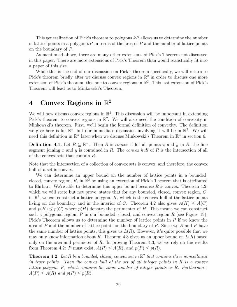
We can determine an upper bound on the number of lattice points in a bounded,closed, convex region, R, in R2 by using an extension of Pick’s Theorem that is attributedto Ehrhart. We’re able to determine this upper bound because R is convex. Theorem 4.2,which we will state but not prove, states that for any bounded, closed, convex region, C,in R2, we can construct a lattice polygon, H, which is the convex hull of the lattice pointsliving on the boundary and in the interior of C. Theorem 4.2 also gives A(H) ≤ A(C)and p(H) ≤ p(C) where p(H) denotes the perimenter of H. This means we can constructsuch a polygonal region, P in our bounded, closed, and convex region R (see Figure 19).Pick’s Theorem allows us to determine the number of lattice points in P if we know thearea of P and the number of lattice points on the boundary of P . Since we R and P havethe same number of lattice points, this gives us L(R). However, it’s quite possible that wemay only know information about R. Theorem 4.3 gives us an upper bound on L(R) basedonly on the area and perimeter of R. In proving Theorem 4.3, we we rely on the resultsfrom Theorem 4.2: P must exist, A(P ) ≤ A(R), and p(P ) ≤ p(R).

Theorem 4.2. Let R be a bounded, closed, convex set in R2 that contains three noncollinearin teger points. Then the convex hull of the set of all integer points in R is a convexlattice polygon, P , which contains the same number of integer points as R. Furthermore,A(P ) ≤ A(R) and p(P ) ≤ p(R).

29

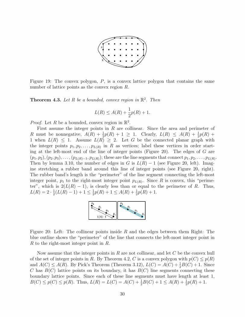
Figure 19: The convex polygon, P , is a convex lattice polygon that contains the samenumber of lattice points as the convex region R.

Theorem 4.3. Let R be a bounded, convex region in R2. Then

L(R) ≤ A(R) +1

2p(R) + 1.

Proof. Let R be a bounded, convex region in R2.First assume the integer points in R are collinear. Since the area and perimeter of

R must be nonnegative, A(R) + 12p(R) + 1 ≥ 1. Clearly, L(R) ≤ A(R) + 1

2p(R) +

1 when L(R) ≤ 1. Assume L(R) ≥ 2. Let G be the connected planar graph withthe integer points p1, p2, . . . , pL(R) in R as vertices; label these vertices in order start-ing at the left-most end of the line of integer points (Figure 20). The edges of G are(p1, p2), (p2, p3), . . . , (pL(R)−1, pL(R)); these are the line segments that connect p1, p2, . . . , pL(R).Then by lemma 3.10, the number of edges in G is L(R) − 1 (see Figure 20, left). Imag-ine stretching a rubber band around this line of integer points (see Figure 20, right).The rubber band’s length is the “perimeter” of the line segment connecting the left-mostinteger point, p1 to the right-most integer point pL(R). Since R is convex, this “perime-ter”, which is 2(L(R) − 1), is clearly less than or equal to the perimeter of R. Thus,L(R) = 2 · 1

2(L(R)− 1) + 1 ≤ 1

2p(R) + 1 ≤ A(R) + 1

2p(R) + 1.

Figure 20: Left: The collinear points inside R and the edges between them Right: Theblue outline shows the “perimeter” of the line that connects the left-most integer point inR to the right-most integer point in R.

Now assume that the integer points in R are not collinear, and let C be the convex hullof the set of integer points in R. By Theorem 4.2, C is a convex polygon with p(C) ≤ p(R)and A(C) ≤ A(R). By Pick’s Theorem (Theorem 3.12), L(C) = A(C) + 1

2B(C) + 1. Since

C has B(C) lattice points on its boundary, it has B(C) line segments connecting theseboundary lattice points. Since each of these line segments must have length at least 1,B(C) ≤ p(C) ≤ p(R). Thus, L(R) = L(C) = A(C) + 1

2B(C) + 1 ≤ A(R) + 1

2p(R) + 1.

30

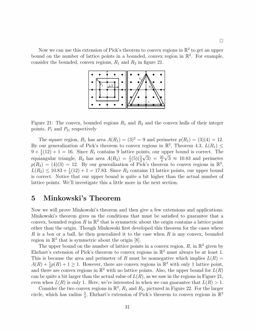
Now we can use this extension of Pick’s theorem to convex regions in R2 to get an upperbound on the number of lattice points in a bounded, convex region in R2. For example,consider the bounded, convex regions, R1 and R2 in figure 21.

Figure 21: The convex, bounded regions R1 and R2 and the convex hulls of their integerpoints, P1 and P2, respectively

The square region, R1 has area A(R1) = (3)2 = 9 and perimeter p(R1) = (3)(4) = 12.By our generalization of Pick’s theorem to convex regions in R2, Theorem 4.3, L(R1) ≤9 + 1

2(12) + 1 = 16. Since R1 contains 9 lattice points, our upper bound is correct. The

equiangular triangle, R2 has area A(R2) = 12(5)(5

2

√3) = 25

4

√3 ≈ 10.83 and perimeter

p(R2) = (4)(3) = 12. By our generalization of Pick’s theorem to convex regions in R2,L(R2) ≤ 10.83 + 1

2(12) + 1 = 17.83. Since R2 contains 13 lattice points, our upper bound

is correct. Notice that our upper bound is quite a bit higher than the actual number oflattice points. We’ll investigate this a little more in the next section.

5 Minkowski’s Theorem

Now we will prove Minkowski’s theorem and then give a few extensions and applications.Minkowski’s theorem gives us the conditions that must be satisfied to guarantee that aconvex, bounded region R in R2 that is symmetric about the origin contains a lattice pointother than the origin. Though Minkowski first developed this theorem for the cases whereR is a box or a ball, he then generalized it to the case when R is any convex, boundedregion in R2 that is symmetric about the origin [8].

The upper bound on the number of lattice points in a convex region, R, in R2 given byEhrhart’s extension of Pick’s theorem to convex regions in R2 must always be at least 1.This is because the area and perimeter of R must be nonnegative which implies L(R) =A(R) + 1

2p(R) + 1 ≥ 1. However, there are convex regions in R2 with only 1 lattice point,

and there are convex regions in R2 with no lattice points. Also, the upper bound for L(R)can be quite a bit larger than the actual value of L(R), as we saw in the regions in Figure 21,even when L(R) is only 1. Here, we’re interested in when we can guarantee that L(R) > 1.

Consider the two convex regions in R2, R1 and R2, pictured in Figure 22. For the largercircle, which has radius 5

4, Ehrhart’s extension of Pick’s theorem to convex regions in R2

31

yields L(R1) ≤ A(R1) + 12p(R1) + 1 = 25

16π + 1

2· 5

2π + 1 = 45

16π + 1 ≈ 9.84. This means there

are 9 or fewer lattice points in R1. Similarly, the same extension of Pick’s theorem yieldsL(R2) ≤ A(R2) + 1

2p(R2) + 1 = 49

64π + 1

2· 7

4π + 1 = 105

64π + 1 ≈ 6.15. This means that there

are 6 or fewer lattice points in R2. However, we can see from Figure 22 that there are 5lattice points in R1, so L(P ) = 5 and that there are no lattice points other than the originin R2, so L(P ) = 1. In both cases, the actual value of L(R) is quite a bit smaller thanour upper bound. How can we gain more information about the actual number of latticepoints in a convex region in R2? More specifically, can we at least determine when L(R)will be at least 1 based on a minimum amount of information?

Figure 22: Two convex regions in R2

Minkowski’s Theorem gives us a simple way to determine whether a given convex regionin R2 that is symmetric about the origin, as are R1 and R2, is guaranteed to contain alattice point other than the origin. This is very useful in proving theorems involving asituation where we need to be sure that there is at least one lattice point in a convexplanar region, but we don’t know everything about the region. We’ll give two examples ofthis usefulness of Minkowski’s Theorem in section 5.3 when we discuss the Two SquaresTheorem and an applied problem, the Orchard Problem. We’ll begin our discussion ofMinkowski’s Theorem with a definition and a few notes on notation. As with our definitionfor convexity, this definition is for Rn, but we will use it in R2 now and in Rn later.

Definition 5.1. A set, R in Rn is symmetric about the origin if whenever the point(x1, x2, . . . , xn) is in R, the point (−x1,−x2, . . . ,−xn) is also in R.

Minkowski’s theorem will only apply to regions that are symmetric about the origin.However, since translation is a plane isometry, we can translate any region that is symmetricabout some other lattice point to the origin while leaving its area and the number of latticepoints it contains unchanged. This allows us to apply Minkowski’s theorem to regions thatare symmetric about other lattice points.

Our proof of Minkowski’s theorem will rely on translations of points in R2, so we willdefine our notation for these translations here. Let R be a set in R2, and let p be a point inR2. We denote the image of the set R under the translation that takes the origin to p byR + p. Taking p to the origin is denoted by R− p. Now we are ready to prove Minkowski’sTheorem.

32

5.1 Proving Minkowski’s Theorem

There are many proofs of Minkowski’s theorem. The one we give here, like many others,relies on Blichfeldt’s lemma, which we prove now.

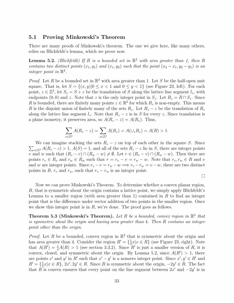
Lemma 5.2. (Blichfeldt) If R is a bounded set in R2 with area greater than 1, then Rcontains two distinct points (x1, y1) and (x1, y2) such that the point (x2 − x1, y2 − y1) is aninteger point in R2.

Proof. Let R be a bounded set in R2 with area greater than 1. Let S be the half-open unitsquare. That is, let S = {(x, y)|0 ≤ x < 1 and 0 ≤ y < 1} (see Figure 23, left). For eachpoint, z ∈ Z2, let Sz = S + z be the translation of S along the lattice line segment lz, withendpoints (0, 0) and z. Note that z is the only integer point in Sz. Let Rz = R∩ Sz. SinceR is bounded, there are finitely many points z ∈ R2 for which Rz is non-empty. This meansR is the disjoint union of finitely many of the sets Rz. Let Rz − z be the translation of Rz

along the lattice line segment lz. Note that Rz − z is in S for every z. Since translation isa plane isometry, it preserves area, so A(Rz − z) = A(Rz). Thus,∑

z∈Z2

A(Rz − z) =∑z∈Z2

A(Rz) = A(∪zRz) = A(R) > 1.

We can imagine stacking the sets Rz − z on top of each other in the square S. Since∑z∈Z2 A(Rz − z) > 1, A(S) = 1, and all of the sets Rz − z lie in S, there are integer points

v and w such that (Rv − v) ∩ (Rw −w) 6= ∅. Let r ∈ (Rv − v) ∩ (Rw −w). Then there arepoints rv ∈ Rv and rw ∈ Rw such that r = rv − v = rw − w. Note that rv, rw ∈ R and vand w are integer points. Since rv− v = rw−w =⇒ rv− rw = v−w, there are two distinctpoints in R, rv and rw, such that rv − rw is an integer point.

Now we can prove Minkowski’s Theorem. To determine whether a convex planar region,R, that is symmetric about the origin contains a lattice point, we simply apply Blichfeldt’sLemma to a smaller region (with area greater than 1) contained in R to find an integerpoint that is the difference under vector addition of two points in the smaller region. Oncewe show this integer point is in R, we’re done. The proof goes as follows.

Theorem 5.3 (Minkowski’s Theorem). Let R be a bounded, convex region in R2 thatis symmetric about the origin and having area greater than 4. Then R contains an integerpoint other than the origin.

Proof. Let R be a bounded, convex region in R2 that is symmetric about the origin andhas area greater than 4. Consider the region R′ = {1

2x|x ∈ R} (see Figure 23, right). Note

that A(R′) = 14A(R) > 1 (see section 3.3.2). Since R′ is just a smaller version of R, it is

convex, closed, and symmetric about the origin. By Lemma 5.2, since A(R′) > 1, thereare points x′ and y′ in R′ such that x′ − y′ is a nonzero integer point. Since x′, y′ ∈ R′ andR′ = {1

2x|x ∈ R}, 2x′, 2y′ ∈ R. Since R is symmetric about the origin, −2y′ ∈ R. The fact

that R is convex ensures that every point on the line segment between 2x′ and −2y′ is in

33

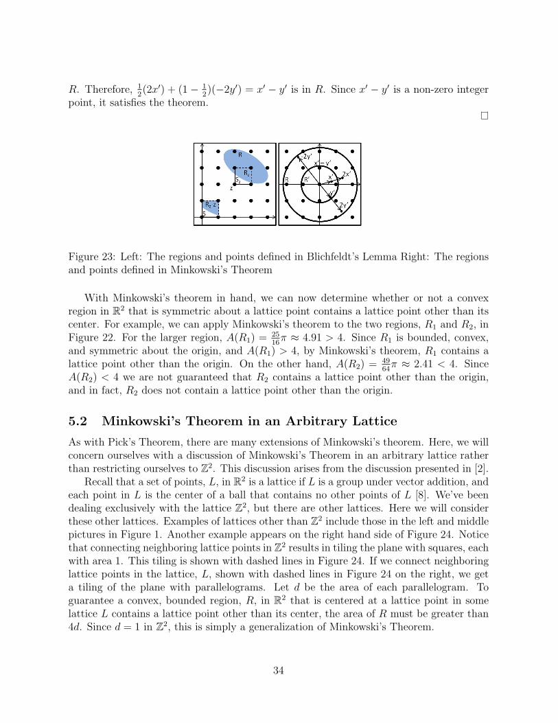
R. Therefore, 12(2x′) + (1 − 1

2)(−2y′) = x′ − y′ is in R. Since x′ − y′ is a non-zero integer

point, it satisfies the theorem.

Figure 23: Left: The regions and points defined in Blichfeldt’s Lemma Right: The regionsand points defined in Minkowski’s Theorem

With Minkowski’s theorem in hand, we can now determine whether or not a convexregion in R2 that is symmetric about a lattice point contains a lattice point other than itscenter. For example, we can apply Minkowski’s theorem to the two regions, R1 and R2, inFigure 22. For the larger region, A(R1) = 25

16π ≈ 4.91 > 4. Since R1 is bounded, convex,

and symmetric about the origin, and A(R1) > 4, by Minkowski’s theorem, R1 contains alattice point other than the origin. On the other hand, A(R2) = 49

64π ≈ 2.41 < 4. Since

A(R2) < 4 we are not guaranteed that R2 contains a lattice point other than the origin,and in fact, R2 does not contain a lattice point other than the origin.

5.2 Minkowski’s Theorem in an Arbitrary Lattice

As with Pick’s Theorem, there are many extensions of Minkowski’s theorem. Here, we willconcern ourselves with a discussion of Minkowski’s Theorem in an arbitrary lattice ratherthan restricting ourselves to Z2. This discussion arises from the discussion presented in [2].

Recall that a set of points, L, in R2 is a lattice if L is a group under vector addition, andeach point in L is the center of a ball that contains no other points of L [8]. We’ve beendealing exclusively with the lattice Z2, but there are other lattices. Here we will considerthese other lattices. Examples of lattices other than Z2 include those in the left and middlepictures in Figure 1. Another example appears on the right hand side of Figure 24. Noticethat connecting neighboring lattice points in Z2 results in tiling the plane with squares, eachwith area 1. This tiling is shown with dashed lines in Figure 24. If we connect neighboringlattice points in the lattice, L, shown with dashed lines in Figure 24 on the right, we geta tiling of the plane with parallelograms. Let d be the area of each parallelogram. Toguarantee a convex, bounded region, R, in R2 that is centered at a lattice point in somelattice L contains a lattice point other than its center, the area of R must be greater than4d. Since d = 1 in Z2, this is simply a generalization of Minkowski’s Theorem.

34

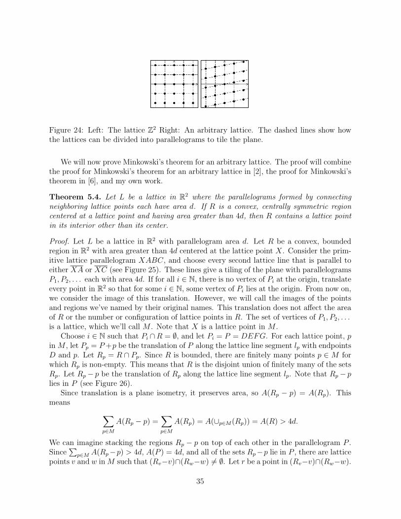
Figure 24: Left: The lattice Z2 Right: An arbitrary lattice. The dashed lines show howthe lattices can be divided into parallelograms to tile the plane.

We will now prove Minkowski’s theorem for an arbitrary lattice. The proof will combinethe proof for Minkowski’s theorem for an arbitrary lattice in [2], the proof for Minkowski’stheorem in [6], and my own work.

Theorem 5.4. Let L be a lattice in R2 where the parallelograms formed by connectingneighboring lattice points each have area d. If R is a convex, centrally symmetric regioncentered at a lattice point and having area greater than 4d, then R contains a lattice pointin its interior other than its center.

Proof. Let L be a lattice in R2 with parallelogram area d. Let R be a convex, boundedregion in R2 with area greater than 4d centered at the lattice point X. Consider the prim-itive lattice parallelogram XABC, and choose every second lattice line that is parallel toeither XA or XC (see Figure 25). These lines give a tiling of the plane with parallelogramsP1, P2, . . . each with area 4d. If for all i ∈ N, there is no vertex of Pi at the origin, translateevery point in R2 so that for some i ∈ N, some vertex of Pi lies at the origin. From now on,we consider the image of this translation. However, we will call the images of the pointsand regions we’ve named by their original names. This translation does not affect the areaof R or the number or configuration of lattice points in R. The set of vertices of P1, P2, . . .is a lattice, which we’ll call M . Note that X is a lattice point in M .

Choose i ∈ N such that Pi ∩R = ∅, and let Pi = P = DEFG. For each lattice point, pin M , let Pp = P +p be the translation of P along the lattice line segment lp with endpointsD and p. Let Rp = R ∩ Pp. Since R is bounded, there are finitely many points p ∈ M forwhich Rp is non-empty. This means that R is the disjoint union of finitely many of the setsRp. Let Rp− p be the translation of Rp along the lattice line segment lp. Note that Rp− plies in P (see Figure 26).

Since translation is a plane isometry, it preserves area, so A(Rp − p) = A(Rp). Thismeans ∑

p∈M

A(Rp − p) =∑p∈M

A(Rp) = A(∪p∈M(Rp)) = A(R) > 4d.

We can imagine stacking the regions Rp − p on top of each other in the parallelogram P .Since

∑p∈M A(Rp−p) > 4d, A(P ) = 4d, and all of the sets Rp−p lie in P , there are lattice

points v and w in M such that (Rv−v)∩(Rw−w) 6= ∅. Let r be a point in (Rv−v)∩(Rw−w).

35

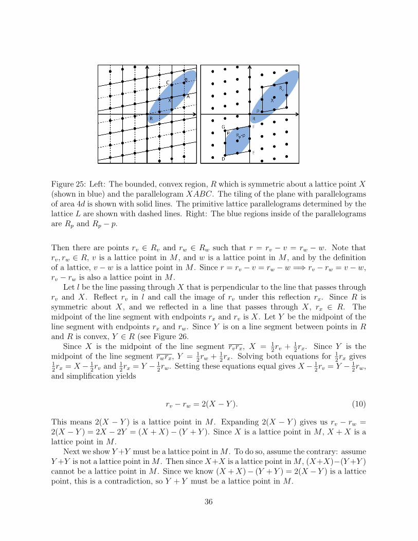
Figure 25: Left: The bounded, convex region, R which is symmetric about a lattice point X(shown in blue) and the parallelogram XABC. The tiling of the plane with parallelogramsof area 4d is shown with solid lines. The primitive lattice parallelograms determined by thelattice L are shown with dashed lines. Right: The blue regions inside of the parallelogramsare Rp and Rp − p.

Then there are points rv ∈ Rv and rw ∈ Rw such that r = rv − v = rw − w. Note thatrv, rw ∈ R, v is a lattice point in M , and w is a lattice point in M , and by the definitionof a lattice, v −w is a lattice point in M . Since r = rv − v = rw −w =⇒ rv − rw = v −w,rv − rw is also a lattice point in M .

Let l be the line passing through X that is perpendicular to the line that passes throughrv and X. Reflect rv in l and call the image of rv under this reflection rx. Since R issymmetric about X, and we reflected in a line that passes through X, rx ∈ R. Themidpoint of the line segment with endpoints rx and rv is X. Let Y be the midpoint of theline segment with endpoints rx and rw. Since Y is on a line segment between points in Rand R is convex, Y ∈ R (see Figure 26.

Since X is the midpoint of the line segment rvrx, X = 12rv + 1

2rx. Since Y is the

midpoint of the line segment rwrx, Y = 12rw + 1

2rx. Solving both equations for 1

2rx gives

12rx = X− 1

2rv and 1

2rx = Y − 1

2rw. Setting these equations equal gives X− 1

2rv = Y − 1

2rw,

and simplification yields

rv − rw = 2(X − Y ). (10)

This means 2(X − Y ) is a lattice point in M . Expanding 2(X − Y ) gives us rv − rw =2(X − Y ) = 2X − 2Y = (X + X)− (Y + Y ). Since X is a lattice point in M , X + X is alattice point in M .

Next we show Y +Y must be a lattice point in M . To do so, assume the contrary: assumeY +Y is not a lattice point in M . Then since X+X is a lattice point in M , (X+X)−(Y +Y )cannot be a lattice point in M . Since we know (X + X)− (Y + Y ) = 2(X − Y ) is a latticepoint, this is a contradiction, so Y + Y must be a lattice point in M .

36

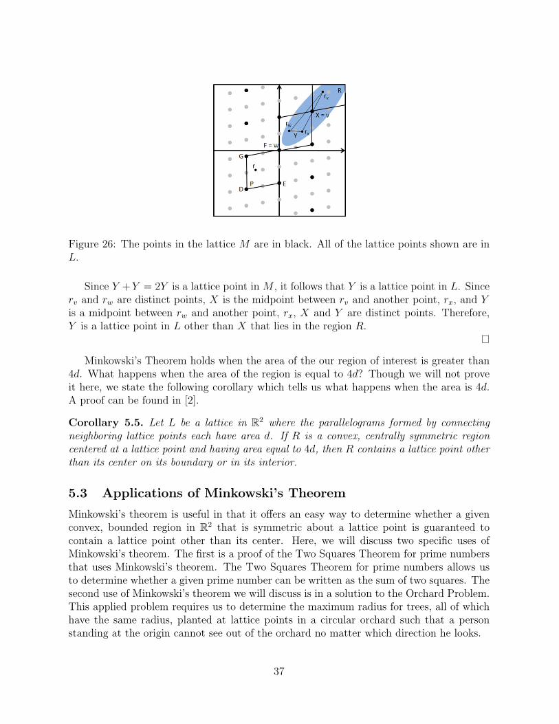
Figure 26: The points in the lattice M are in black. All of the lattice points shown are inL.

Since Y +Y = 2Y is a lattice point in M , it follows that Y is a lattice point in L. Sincerv and rw are distinct points, X is the midpoint between rv and another point, rx, and Yis a midpoint between rw and another point, rx, X and Y are distinct points. Therefore,Y is a lattice point in L other than X that lies in the region R.

Minkowski’s Theorem holds when the area of the our region of interest is greater than4d. What happens when the area of the region is equal to 4d? Though we will not proveit here, we state the following corollary which tells us what happens when the area is 4d.A proof can be found in [2].

Corollary 5.5. Let L be a lattice in R2 where the parallelograms formed by connectingneighboring lattice points each have area d. If R is a convex, centrally symmetric regioncentered at a lattice point and having area equal to 4d, then R contains a lattice point otherthan its center on its boundary or in its interior.

5.3 Applications of Minkowski’s Theorem

Minkowski’s theorem is useful in that it offers an easy way to determine whether a givenconvex, bounded region in R2 that is symmetric about a lattice point is guaranteed tocontain a lattice point other than its center. Here, we will discuss two specific uses ofMinkowski’s theorem. The first is a proof of the Two Squares Theorem for prime numbersthat uses Minkowski’s theorem. The Two Squares Theorem for prime numbers allows usto determine whether a given prime number can be written as the sum of two squares. Thesecond use of Minkowski’s theorem we will discuss is in a solution to the Orchard Problem.This applied problem requires us to determine the maximum radius for trees, all of whichhave the same radius, planted at lattice points in a circular orchard such that a personstanding at the origin cannot see out of the orchard no matter which direction he looks.

37

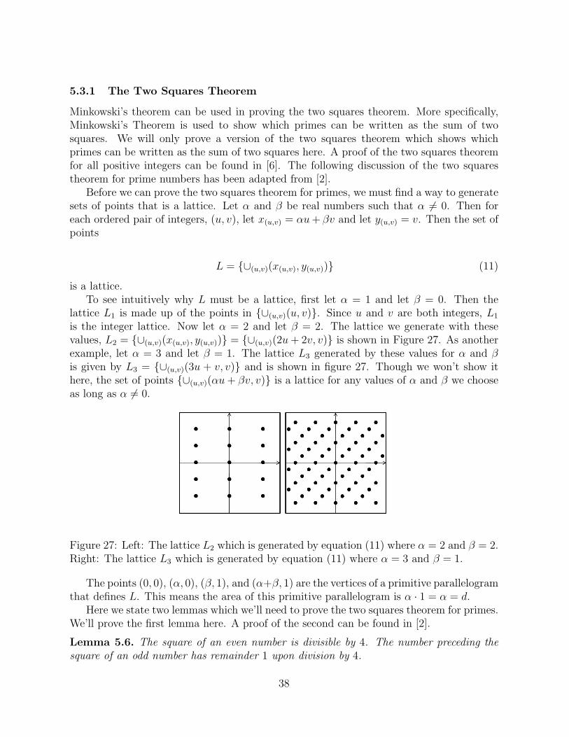
5.3.1 The Two Squares Theorem

Minkowski’s theorem can be used in proving the two squares theorem. More specifically,Minkowski’s Theorem is used to show which primes can be written as the sum of twosquares. We will only prove a version of the two squares theorem which shows whichprimes can be written as the sum of two squares here. A proof of the two squares theoremfor all positive integers can be found in [6]. The following discussion of the two squarestheorem for prime numbers has been adapted from [2].

Before we can prove the two squares theorem for primes, we must find a way to generatesets of points that is a lattice. Let α and β be real numbers such that α 6= 0. Then foreach ordered pair of integers, (u, v), let x(u,v) = αu + βv and let y(u,v) = v. Then the set ofpoints

L = {∪(u,v)(x(u,v), y(u,v))} (11)

is a lattice.To see intuitively why L must be a lattice, first let α = 1 and let β = 0. Then the

lattice L1 is made up of the points in {∪(u,v)(u, v)}. Since u and v are both integers, L1

is the integer lattice. Now let α = 2 and let β = 2. The lattice we generate with thesevalues, L2 = {∪(u,v)(x(u,v), y(u,v))} = {∪(u,v)(2u + 2v, v)} is shown in Figure 27. As anotherexample, let α = 3 and let β = 1. The lattice L3 generated by these values for α and βis given by L3 = {∪(u,v)(3u + v, v)} and is shown in figure 27. Though we won’t show ithere, the set of points {∪(u,v)(αu + βv, v)} is a lattice for any values of α and β we chooseas long as α 6= 0.

Figure 27: Left: The lattice L2 which is generated by equation (11) where α = 2 and β = 2.Right: The lattice L3 which is generated by equation (11) where α = 3 and β = 1.

The points (0, 0), (α, 0), (β, 1), and (α+β, 1) are the vertices of a primitive parallelogramthat defines L. This means the area of this primitive parallelogram is α · 1 = α = d.

Here we state two lemmas which we’ll need to prove the two squares theorem for primes.We’ll prove the first lemma here. A proof of the second can be found in [2].

Lemma 5.6. The square of an even number is divisible by 4. The number preceding thesquare of an odd number has remainder 1 upon division by 4.

38

Proof. Let n be an even number. Then for some integer k, n = 2k. This means n2 =(2k)2 = 4k2. Thus, n2 is divisible by 4.

Let n be an odd number. Then the number preceding the square of n is n2 − 1 =(n + 1)(n− 1). Since n is odd, n + 1 and n− 1 are both even, and therefore (n + 1)(n− 1)is divisible by 4.

Lemma 5.7. Let p be a prime of the form 4k +1. Then there exists an integer c for whichc2 + 1 ≡ 0(mod p).

Theorem 5.8. Let p be a prime number. If p = 2 or p is of the form 4k +1, then p can bewritten as the sum of the squares of two positive integers. If p is of the form 4k + 3, thenp cannot be written as the sum of squares of two positive integers.

Proof. Let p be a prime number such that p = 2 or p = 4k + 1 for some integer k. ByLemma 5.7, there is an integer, a, for which a2 + 1 is divisible by p. Note that when p = 2,such an a exists as well, since (1)2 + 1 = 2 is divisible by 2. Fix a such that a2 + 1 isdivisible by p.

Consider the lattice L where the lattice points (x, y), satisfy x = pu + av and y = vfor u, v ∈ Z. Let d be the area of each of the parallelograms that determine L. From thediscussion above concerning area of the primitive parallelogram that determines a lattice,L, d = p. Since x2 + y2 = p(pu2 + 2auv) + (a2 + 1)v2 and (a2 + 1) is divisible by p, x2 + y2

is divisible by p.

Consider the circle, C, that is centered at the origin with radius 2√

dπ. Since A(C) = 4d,

by Corollary 5.5, there must be a lattice point, (x, y) in the interior or on the boundary ofC that is not the origin. Fix such a lattice point, and call it (x, y). Since (x, y) is eitheron the boundary of C or in the interior of C, (x, y) must satisfy x2 + y2 ≤ 4d

π= 4p

π< 2p.

Since (x, y) is not the origin, x2 + y2 must be positive. Since x2 + y2 is divisible by p andis less than 2p, it must be the case that x2 + y2 = p. Thus, since x and y are integers, pcan be written as the sum of two squares.

For the second part of the theorem, let p be a prime number so that p = 4k + 3 forsome integer k. By Lemma 5.6, the square of an even number, n is divisible by 4, that is,n2 ≡ 0(mod 4). Also by Lemma 5.6, the number preceding the square of an odd number,m is divisible by 4, that is, m2 ≡ 1(mod 4). This means that for a sum of two squares,s, s ≡ 0(mod 4) when s is the sum of squares of two even integers, s ≡ 1(mod 4) when sis the sum of squares of an even integer and an odd integer, or s ≡ 2 (mod 4) when s isthe sum of squares of two odd integers. However, it is never the case that s ≡ 3 (mod 4).Thus, p is not a sum of two squares.

We can actually use the Two Squares Theorem to gain more information about theinteger lattice, Z2. The only numbers that can be equal to the area of a lattice square inZ2 are integers that can be written as the sum of two squares of positive integers.

39

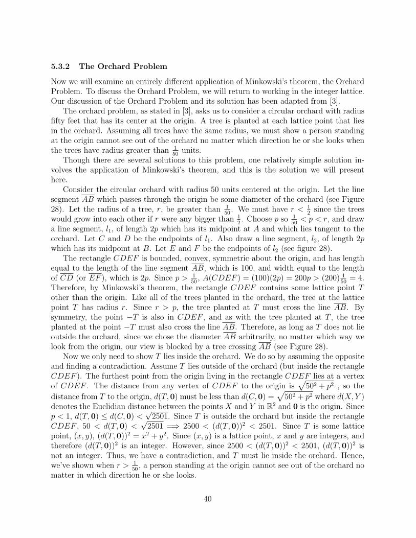
5.3.2 The Orchard Problem

Now we will examine an entirely different application of Minkowski’s theorem, the OrchardProblem. To discuss the Orchard Problem, we will return to working in the integer lattice.Our discussion of the Orchard Problem and its solution has been adapted from [3].

The orchard problem, as stated in [3], asks us to consider a circular orchard with radiusfifty feet that has its center at the origin. A tree is planted at each lattice point that liesin the orchard. Assuming all trees have the same radius, we must show a person standingat the origin cannot see out of the orchard no matter which direction he or she looks whenthe trees have radius greater than 1

50units.

Though there are several solutions to this problem, one relatively simple solution in-volves the application of Minkowski’s theorem, and this is the solution we will presenthere.

Consider the circular orchard with radius 50 units centered at the origin. Let the linesegment AB which passes through the origin be some diameter of the orchard (see Figure28). Let the radius of a tree, r, be greater than 1

50. We must have r < 1

2since the trees

would grow into each other if r were any bigger than 12. Choose p so 1

50< p < r, and draw

a line segment, l1, of length 2p which has its midpoint at A and which lies tangent to theorchard. Let C and D be the endpoints of l1. Also draw a line segment, l2, of length 2pwhich has its midpoint at B. Let E and F be the endpoints of l2 (see figure 28).

The rectangle CDEF is bounded, convex, symmetric about the origin, and has lengthequal to the length of the line segment AB, which is 100, and width equal to the lengthof CD (or EF ), which is 2p. Since p > 1

50, A(CDEF ) = (100)(2p) = 200p > (200) 1

50= 4.

Therefore, by Minkowski’s theorem, the rectangle CDEF contains some lattice point Tother than the origin. Like all of the trees planted in the orchard, the tree at the latticepoint T has radius r. Since r > p, the tree planted at T must cross the line AB. Bysymmetry, the point −T is also in CDEF , and as with the tree planted at T , the treeplanted at the point −T must also cross the line AB. Therefore, as long as T does not lieoutside the orchard, since we chose the diameter AB arbitrarily, no matter which way welook from the origin, our view is blocked by a tree crossing AB (see Figure 28).

Now we only need to show T lies inside the orchard. We do so by assuming the oppositeand finding a contradiction. Assume T lies outside of the orchard (but inside the rectangleCDEF ). The furthest point from the origin living in the rectangle CDEF lies at a vertexof CDEF . The distance from any vertex of CDEF to the origin is

√502 + p2 , so the

distance from T to the origin, d(T,0) must be less than d(C,0) =√

502 + p2 where d(X, Y )denotes the Euclidian distance between the points X and Y in R2 and 0 is the origin. Sincep < 1, d(T,0) ≤ d(C,0) <

√2501. Since T is outside the orchard but inside the rectangle

CDEF , 50 < d(T,0) <√

2501 =⇒ 2500 < (d(T,0))2 < 2501. Since T is some latticepoint, (x, y), (d(T,0))2 = x2 + y2. Since (x, y) is a lattice point, x and y are integers, andtherefore (d(T,0))2 is an integer. However, since 2500 < (d(T,0))2 < 2501, (d(T,0))2 isnot an integer. Thus, we have a contradiction, and T must lie inside the orchard. Hence,we’ve shown when r > 1

50, a person standing at the origin cannot see out of the orchard no

matter in which direction he or she looks.

40

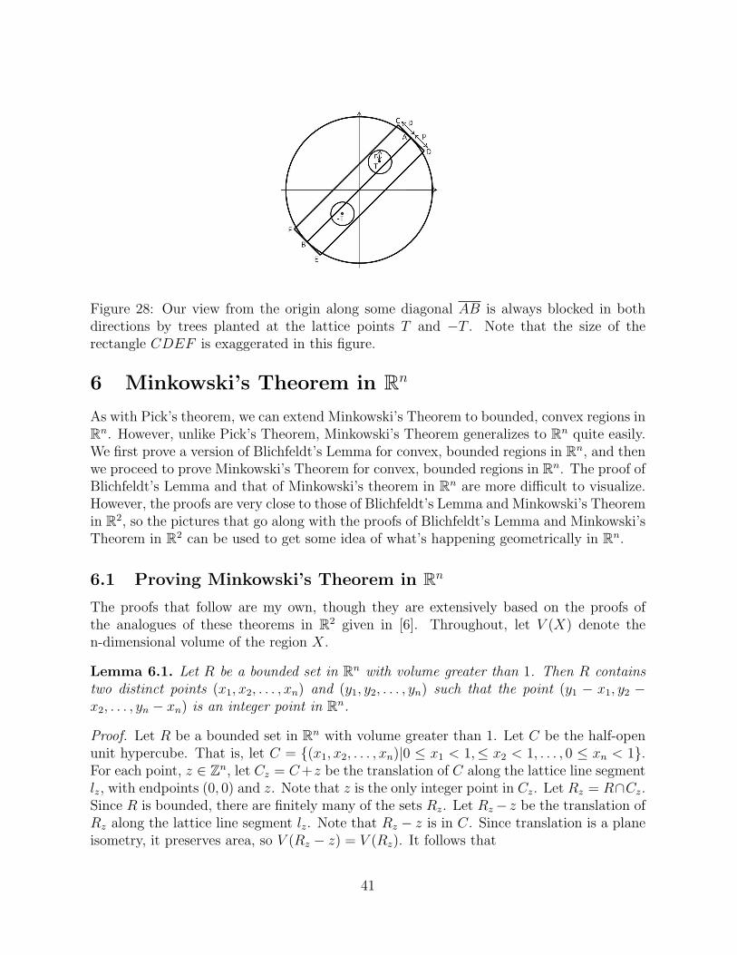
Figure 28: Our view from the origin along some diagonal AB is always blocked in bothdirections by trees planted at the lattice points T and −T . Note that the size of therectangle CDEF is exaggerated in this figure.

6 Minkowski’s Theorem in Rn

As with Pick’s theorem, we can extend Minkowski’s Theorem to bounded, convex regions inRn. However, unlike Pick’s Theorem, Minkowski’s Theorem generalizes to Rn quite easily.We first prove a version of Blichfeldt’s Lemma for convex, bounded regions in Rn, and thenwe proceed to prove Minkowski’s Theorem for convex, bounded regions in Rn. The proof ofBlichfeldt’s Lemma and that of Minkowski’s theorem in Rn are more difficult to visualize.However, the proofs are very close to those of Blichfeldt’s Lemma and Minkowski’s Theoremin R2, so the pictures that go along with the proofs of Blichfeldt’s Lemma and Minkowski’sTheorem in R2 can be used to get some idea of what’s happening geometrically in Rn.

6.1 Proving Minkowski’s Theorem in Rn

The proofs that follow are my own, though they are extensively based on the proofs ofthe analogues of these theorems in R2 given in [6]. Throughout, let V (X) denote then-dimensional volume of the region X.

Lemma 6.1. Let R be a bounded set in Rn with volume greater than 1. Then R containstwo distinct points (x1, x2, . . . , xn) and (y1, y2, . . . , yn) such that the point (y1 − x1, y2 −x2, . . . , yn − xn) is an integer point in Rn.

Proof. Let R be a bounded set in Rn with volume greater than 1. Let C be the half-openunit hypercube. That is, let C = {(x1, x2, . . . , xn)|0 ≤ x1 < 1,≤ x2 < 1, . . . , 0 ≤ xn < 1}.For each point, z ∈ Zn, let Cz = C +z be the translation of C along the lattice line segmentlz, with endpoints (0, 0) and z. Note that z is the only integer point in Cz. Let Rz = R∩Cz.Since R is bounded, there are finitely many of the sets Rz. Let Rz− z be the translation ofRz along the lattice line segment lz. Note that Rz − z is in C. Since translation is a planeisometry, it preserves area, so V (Rz − z) = V (Rz). It follows that

41

∑z∈Zn

V (Rz − z) =∑z∈Zn

V (Rz) = V (∪z∈Zn(Rz)) = V (R) > 1.

We can imagine placing all of the sets Rz−z together in C. Since∑

z∈Zn V (Rz−z) > 1,V (C) = 1, and all of the sets Rz − z are in C, there are integer points v and w such that(Rv − v) ∩ (Rw − w) 6= ∅. Let r ∈ (Rv − v) ∩ (Rw − w). Then there are points rv ∈ Rv

and rw ∈ Rw such that r = rv − v = rw −w. Note that rv, rw ∈ R and v and w are integerpoints. Since rv − v = rw − w =⇒ rv − rw = v − w, there are two distinct points in R, rv

and rw, such that rv − rw is an integer point.

We will need one additional fact to prove Minkowski’s Theorem in Rn. Recall thatwhen length in a region, R, in R2 is changed by a factor of k, the area of R is changed bya factor of k2 where k is a positive real number. Similarly, when length in a region, R inRn is changed by a factor of k, the volume of R is changed by a factor of kn. As with thecase in two dimensions, this can be shown using linear algebra. Let M : Rn → Rn be thelinear transformation given by Mx = nx where x is a vector in Rn emanating from theorigin with endpoint at a lattice point and M is the n× n matrix

M =

k 0 . . . 00 k . . . 0

. . . . . .0 0 . . . k

.

Under M , the vector v = 〈x1, x2, . . . , xn〉 is mapped to the vector kv = 〈kx1, kx2, . . . , kxn〉 =k〈x1, x2, . . . , xn〉 which results in the length of the vector v changing by a factor of k. Sincedet(M) = kn, the volume of the image of any bounded region, R, in Rn is different fromthe volume of R by a factor of kn.

Theorem 6.2. If R is a bounded, convex region in Rn having volume greater than 2n andis symmetric about the origin, then R contains an integer point other than the origin.

Proof. Let R be a bounded, convex region in Rn that is symmetric about the origin andhas volume greater than 2n. Consider the region R′ = {1

2x|x ∈ R}. Note that V (R′) =

12n V (R) > 1. Since R′ is just a smaller version of R, it is convex, closed, and symmetricabout the origin. It follows that since V (R′) > 1, by Lemma 6.1, there are points x′ and y′

in R′ such that x′ − y′ is a nonzero integer point. Since x′, y′ ∈ R′ and R′ = {12x|x ∈ R},

2x′, 2y′ ∈ R. Since R is symmetric about the origin, −2y′ ∈ R. The fact that R is convexensures that every point on the line segment between 2x′ and −2y′ is in R. Therefore,12(2x′)+ (1− 1

2)(−2y′) = x′− y′ is in R. Since x′− y′ is a non-zero integer point, it satisfies

the theorem.

Though we will not pursue it here, it is possible to prove Minkowski’s theorem for anarbitrary lattice in Rn. Those interested in the proof should see [8].

42

6.2 Applications of Minkowski’s Theorem in Rn

As with Minkowski’s theorem in R2, there are many applications of Minkowski’s theoremin Rn. Though we won’t elaborate on any of these applications here, we will list a few ofthem.

First, there are many fundamental facts in algebraic number theory which can be provedusing Minkowski’s theorem in Rn [7]. There are also some more elementary results innumber theory that can be obtained using Minkowski’s lattice point theorem in Rn. Theseinclude the Four Squares Theorem, which states that every natural number can be writtenas the sum of four squares of nonnegative integers, and a theorem from Legendre that givesthe conditions under which the equation ax2 +by2 +cz2 = 0, where a, b, and c are relativelyprime, square-free integers which do not all have the same sign, has non-trivial solutions[7].

7 Conclusions

We’ve employed some basic facts and definitions about lattices to investigate two theorems,Pick’s Theorem and Minkowski’s Theorem. Both Pick’s theorem and Minkowski’s Theoremhave a very wide range of extensions and applications reaching far beyond anything we’vediscussed here. While at first glance, the two theorems seem to address entirely differentquestions, Pick’s theorem involves finding the area of lattice polygons, while Minkowski’sTheorem involves determining when a convex region in R2 centered at a lattice pointcontains a lattice point other than its center, we find through examining extensions of boththeorems that they are more closely related than they seem at first. In the end, both giveus information about the number of lattice points in a particular region, and both haveapplications to other branches of mathematics.

8 Acknowledgements

I would like to thank my advisors Professor Marie Snipes and Professor Judy Holdener foranswering all of my questions regarding the subject matter of this paper and for offeringhelpful feedback on preliminary drafts. I would also like to thank Professor Holdener forher help in choosing a topic for the paper and Yinan Yu for reading and commenting on adraft of the paper.

References

[1] Bridger, Mark, Andrei Zelevinsky. “Visibles Revisited.” The College Mathematics Jour-nal. 36 (2005), 289-300.

[2] Erdos, Paul, Janos Suranyi. Topics in the Theory of Numbers. Translated by BaryGuiduli. New York: Springer, 2003.

43

[3] Honsberger, Ross. “The Orchard Problem.” Biscuits of Number Theory. Edited byArthur Benjamin and Ezra Brown. Washington, D.C.: Mathematical Association ofAmerica, 2009.

[4] Poole, David. Linear Algebra: A Modern Introduction. Australia: Brooks/Cole-Thomson Learning, 2006.

[5] Rotman, Joseph J. A First Course in Abstract Algebra. Upper Saddle River, N.J.:Prentice Hall, 2006.

[6] Sally, Judith D., and Paul Sally. Roots to Research: A Vertical Development of Mathe-matical Problems. Providence, RI: American Mathematical Society, 2007.

[7] Scharlau, Winfried, Hans Opolka. From Fermat to Minkowski: Lectures on the Theoryof Numbers and Its Historical Development. New York: Springer-Verlag, 1985.

[8] Stein, Sherman K., and Sandor Szabo. Algebra and Tiling: Homomorphisms in theService of Geometry. Washington D.C.: Mathematical Association of America, 1994.

[9] Varberg, Dale E. “Pick’s Theorem Revisited.” American Mathematical Monthly. 92(1985), 584-587.

44