Latency Meter: A device to measure end-to-end latency of VE systemsDorian Miller and Gary Bishop

*

University of North Carolina at Chapel Hill

ABSTRACT

The effectiveness of virtual environment systems depends critically on the end-to-end delay between the user's motion

and the update of the display. When the user moves, the graphics system must update the images on the display to reflect

the proper projection of the virtual world on their field of vision. Significant delay in this update is perceived as

swimming of the virtual world; objects in the virtual world appear to follow the user's motions. We are developing a

standalone instrument that quickly estimates end-to-end latency without requiring electrical connections or changes to

the VE software. We believe that a method for easily monitoring latency will change the way programmers and users

work. Our latency meter works by observing the user's motion and the display's response using high-speed optical

sensors. When the user rocks back and forth, the display exhibits a similar but delayed rocking of objects in the user's

field of vision. We process the signals from the optical sensors to extract the times of very slow image change

corresponding to the times when the user is nearly stopped (just before reversing direction). By correlating a sequence of

these turn-around points in the two signals we can accurately estimate the end-to-end system delay.

Keywords: End-to-end latency, System performance, Virtual environments

1. The Problem.Despite dramatic advances in virtually all the components of VE systems – renderers, displays, trackers – the overall

performance of such systems is still hard to measure. Even with careful continuous monitoring of frame rate, for

instance, a system from one day to the next “appears” to perform less well. All too often the change is some trivial detail

whose effect the system doesn’t measure and whose overall impact only the most experienced developers will

understand: a change in the buffering behavior between tracker and host computer, for instance. An experienced user

may realize that “something is wrong”, but has no way to demonstrate or confirm that some deleterious change has

occurred.

The most serious sites perform latency measurements on their systems from time to time for quality control, but these

exercises are difficult and time consuming and their validity doesn’t extend much beyond the isolated situations

measured at the time of the experiment. The following day, for example, a small change in the system –– the orientation

of the user with respect to the simulated or real environment –– may change the execution-time behavior of the system.

We have encountered this problem for years but existing methods for latency measurement were too invasive for

everyday use.

2. Our approach.It is well known that you can evaluate the transfer function of a “black-box” linear system by stimulating its input with a

known signal and examining the resulting output.1 Even more complicated systems with internal state and some non-

linearity can be evaluated in this way. Indeed, existing methods for measuring VE system latency work this way.2,3

For

example, in Mine’s method4, a pendulum provides a controlled stimulus to the system and a photo sensor watches for a

specially programmed response.

We can eliminate the pendulum and the program modifications by simultaneously observing the user’s motion and the

normal displayed response of the system. The top row of figure 1 shows a user, first, rocking toward his right and then to

his left. The bottom row shows the displayed response of the VE system with the manikin image moving relative to the

background in response to the user’s motion. We could use video cameras and well-known computer vision methods for

* {dorianm, gb}@cs.unc.edu; phone (919) 962-1700; http://www.cs.unc.edu; University of North Carolina, CB 3175, Sitterson Hall,

Chapel Hill, NC, 27599-3175

extracting the user’s motion from the first image sequence and the virtual camera motion from the second image

sequence. Then these two motion sequences could be used estimate system delay. This would require a system capable

of simultaneously acquiring and processing two video streams.

3. Simple Sensors.We replace each of the video cameras above with a pair of orthogonally mounted one-dimensional CCD sensors of 128

pixels each. This reduces the amount of data that has to be processed from about 300,000 pixels per frame to only 256

pixels per frame. As a result we can operate the CCD sensors at much higher than video frame rates using a data

acquisition board to digitize the analog output signals. Further, we reduce the 128 samples out of each CCD to a single

number representing the location of the centroid (the center of “mass” of the brightness distribution) on the sensor.

Devices such as lateral-effect photodiodes5 produce this output directly and could be used for this application but CCD

arrays are more readily available and are less expensive. The centroid calculation is given below; I(x) is the intensity for

the pixel at x.

127

0

127

0

( )

( )

x

x

xI xC

I x

=

=

=∑

∑Now we have two streams of numbers (X and Y) from the sensor observing the user and another two streams from the

sensor observing the display. Each of these streams tells us something about the observed scenes along a single

dimension. For example, as the user rocks back and forth the position of the centroid will change. The change in the

centroid will not necessarily correspond in a simple way to the user’s rocking because he may occlude background

objects as he moves. Likewise, when the VE system updates the display in response to the user’s motion the position of

the centroid on its sensor will change.

4. Signal Processing.We cannot count on a simple linear relationship between the X-Y centroid positions for the user and those for the VE

display. But, without restricting the application too much, we can assume that when the user is not moving the centroid

from his sensor will change relatively little. Further when the user is not moving, the VE display (for static VE scenes)

Figure 1: User motion results in corresponding motion in the VE display.

should not change. Thus, by detecting stops (times of little motion) in the user sequence and relating them to the

corresponding stops in the VE sequence we can estimate the system delay.

We compute the change in the centroid position from frame to frame and we combine the X and Y changes to produce

the magnitude of the centroid speed in pixels per second. Rather than finding stops by thresholding, a process that is

subject to noise and gain variations, we convert the speed to a likelihood of being stopped using the ad-hoc equation:

10

1( )

(1 )stop speed

speed=

+When speed is zero (no change since last frame) this function is one, as the speed increases this function rapidly drops to

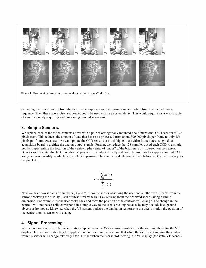
zero. Figure 2a shows the speed signals for a motion sequence and figure 2b shows the corresponding detected stops.

5. Extracting the delay.Finally we correlate a window of a few seconds of the stop signals for the user motion with those from the VE display.

Figure 2c shows the resulting correlation. Because the user motion was regular we get multiple peaks in the correlation.

The first peak corresponding to a positive delay is the one we want. This is a good estimate of the average latency of the

VE system over the window.

Figure 2: Calculating latency from sensor data. a) Speed signals of motion data b) Calculated stops c) Resulting correlation. The peak

at 78 ms is the measured system latency

0 0.5 1 1.5 2 2.50

0.2

0.4

0.6

0.8

1

seconds

spee

d

Input (solid blue) and output (magenta dashed) centroid data

0 0.5 1 1.5 2 2.50

0.2

0.4

0.6

0.8

1

seconds

stop

Input speed (solid blue) and transf orm (dashed magenta)

0 0.1 0.2 0.3 0.4 0.5 0.6 0.7 0.8 0.9 1 1.1 1.2 1.3 1.4 1.5 1.6 1.7 1.8 1.9 2

0

5

10

15

Latency correlation

latency 0.078 sec

ma

tch

0 0.5 1 1.5 2 2.50

0.2

0.4

0.6

0.8

1

seconds

spee

d

Input (solid blue) and output (magenta dashed) centroid data

0 0.5 1 1.5 2 2.50

0.2

0.4

0.6

0.8

1

seconds

spee

d

Input (solid blue) and output (magenta dashed) centroid data

0 0.5 1 1.5 2 2.50

0.2

0.4

0.6

0.8

1

seconds

stop

Input speed (solid blue) and transf orm (dashed magenta)

0 0.5 1 1.5 2 2.50

0.2

0.4

0.6

0.8

1

seconds

stop

Input speed (solid blue) and transf orm (dashed magenta)

0 0.1 0.2 0.3 0.4 0.5 0.6 0.7 0.8 0.9 1 1.1 1.2 1.3 1.4 1.5 1.6 1.7 1.8 1.9 2

0

5

10

15

Latency correlation

latency 0.078 sec

ma

tch

0 0.1 0.2 0.3 0.4 0.5 0.6 0.7 0.8 0.9 1 1.1 1.2 1.3 1.4 1.5 1.6 1.7 1.8 1.9 2

0

5

10

15

Latency correlation

latency 0.078 sec

ma

tch

a)

b)

c)

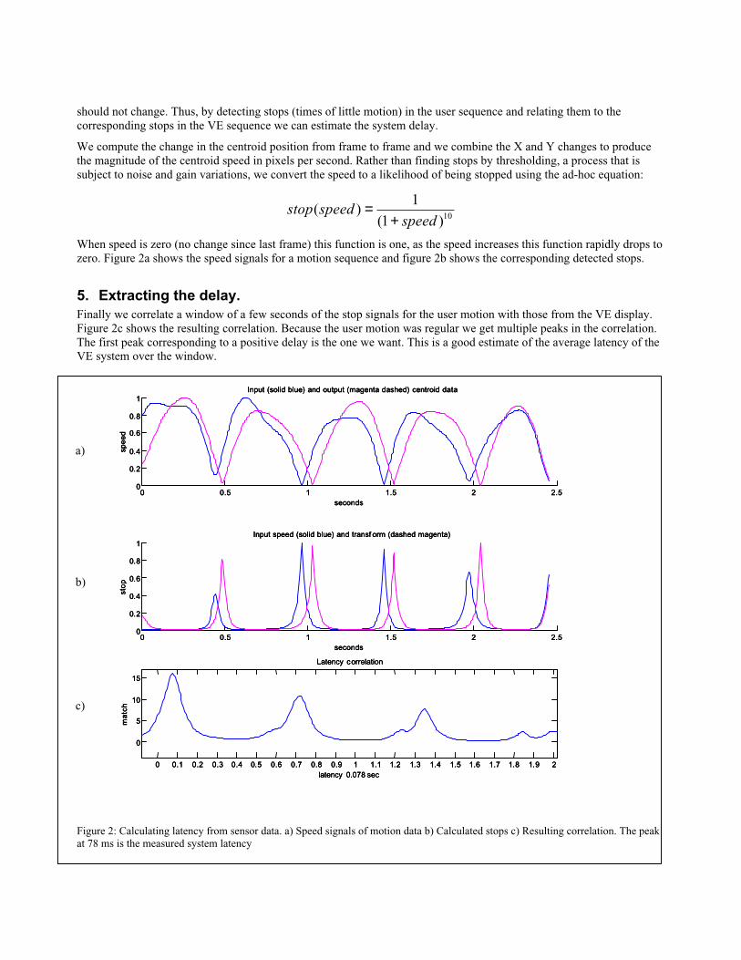
6. PrototypeOur prototype implementation is shown in figures 3 and 4. The sensors each have two TAOS TSL1401 CCD sensors

with 128 pixels each. A cylindrical lens focuses the image onto the array. A National Instruments model PCI-6052E data

acquisition board provides the clock and control signals to the CCD arrays and digitizes their analog output signals. We

use Matlab with the “Data Acquisition Toolbox” running on a 550 MHz PC compatible running Windows NT. The

system acquires data from the CCD arrays with a frame rate of 150 Hz and updates its latency estimate 10 times per

second.

Figure 3: Latency meter in use. User is on the left. Projected output is on the right. The optical sensors of the latency meter are circled.

The sensors are shown in more detail in figure 4.

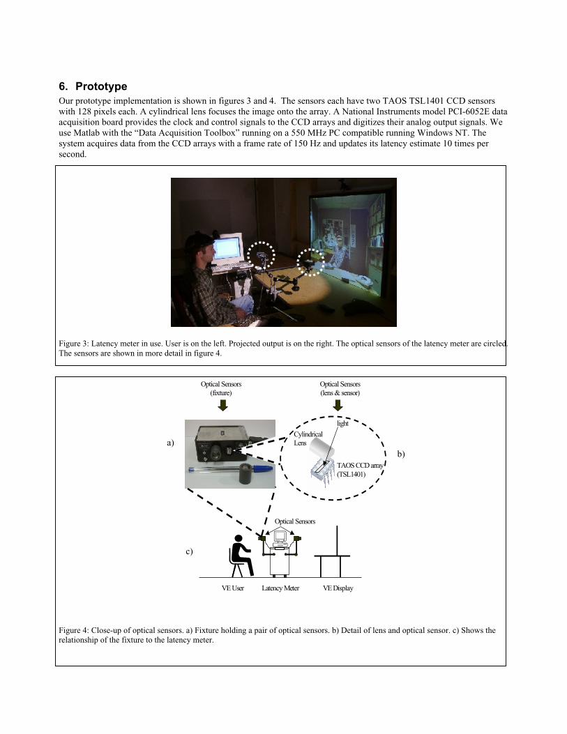
Figure 4: Close-up of optical sensors. a) Fixture holding a pair of optical sensors. b) Detail of lens and optical sensor. c) Shows the

relationship of the fixture to the latency meter.

Optical Sensors

light

TAOS CCD array

(TSL1401)

Cylindrical

Lens

Optical Sensors

(fixture)

Optical Sensors

(lens & sensor)

VE Display VE User Latency Meter

c)

b)

a)

7. Results

We have used the latency meter to measure latencies in five different virtual environment systems. Each of these systems

use an optical, magnetic, or haptic device for tracking the user. Different display technologies used by the systems are

projectors, monitors and head mounted displays (HMD). Rather than attempting to focus the latency meter sensors on

the tiny display of the HMD, we chose to display the system output on an LCD monitor in addition to the HMD. Though

the LCD monitor could conceivably have different delay characteristics than the displays in the HMD, the difference due

to the HMD and the monitor can be measured in a separate experiment. The latency meter results of two systems were

validated using Mine’s method.

The verified interactive systems are used by the Tele-immersion6 and Effective Virtual Environments

7 (EVE) projects.

The Tele-immersion project uses virtual environments for an extension to teleconferencing. In this system, the user sits

across from a projected image of an office at a remote location. Tracking the user’s head with an optical tracker and

projecting a view-dependent stereo gives the impression of looking through a window to see the other participant.

The EVE group investigates making virtual environments as convincing as possible to the user. Their virtual

environment system tracks the user’s head with an optical tracker and presents the images using a HMD. The user walks

through a virtual room and around a realistically rendered pit. For making latency measurements, we redirected the

output of the EVE system to an LCD monitor in addition to the HMD.

Both systems were measured with the latency meter and Mine method. The Mine method validates the results of the

latency meter. The Mine method measures end-to-end system latency by mounting the tracker on a swinging pendulum.

The VE is modified to display a polygon as one color when the pendulum is on one side of zero and as another color

when it is on the other side of zero. End-to-end latency is measured as the time between when the pendulum passes zero

and when the system responds by changing the color of a polygon on the display. Latency is read from an oscilloscope

that displays the output of sensors detecting the two events of the tracker moving through the known location and the

resulting change in polygon color.

The latency meter and Mine method measurements were conducted under identical conditions. Coincidently, both tested

systems use the same optical tracker. The tracking software has a controllable filter parameter, which when increased

also increases system delay. This benefits the user by providing smoother tracking. The measurements are conducted

repeatedly, each time setting the controlled delay parameter from 0 to 250 in steps of 50. The measured systems are

modified in order to perform the Mine experiment. The modifications should make negligible changes to the end-to-end

system latency.

Results for the Tele-immersion and EVE projects are shown in figure 5. The measured system delay is plotted against

the delay value set in the tracking system. The overlapping plots of the latency meter (LM) and Mine method (MM)

confirm that the two independent techniques obtain the same end-to-end latency measurement.

Figure 5: Validation results with Mine method. a) Results of Tele-immersion. b) Results of EVE

0 100 200 3000

50

100

150

200

tracker delay parameter

late

ncy

(ms)

Tele-immersion latency meter validation

LMMM

0 100 200 3000

50

100

150

200

tracker delay parameter

late

ncy

(ms)

Walkthrough latency meter validation

LMMM

a) b)

0 100 200 3000

50

100

150

200

tracker delay parameter

late

ncy

(ms)

Tele-immersion latency meter validation

LMMM

0 100 200 3000

50

100

150

200

tracker delay parameter

late

ncy

(ms)

Walkthrough latency meter validation

LMMM

a) b)

Discrepancies in the overlapping plots are due to experimental error. Measured latencies vary from 50 ms to 150 ms and

are plausible latencies for these systems. The EVE project has approximately 20 ms more latency than the Tele-

immersion project at the equivalent setting. The explanation is that the EVE system’s scene and communication

infrastructure are more complex than the Tele-immersion system.

The following three systems were measured only with the latency meter. They illustrate the variety of systems to which

the latency meter is applicable. The three systems are discussed in order of increasing delay.

The Shader Lamps8 application lets the user paint with a virtual paintbrush onto physical objects. The white-colored

object is tracked using a magnetic tracker and projectors display color images onto the objects. System latency is evident

when the physical object is moved and the projected colors lag behind and thus do not overlap the object. The latency

meter reports the latency of this application as 100 ms.

The NanoManipulator9 project lets the user see and touch an atomic scale surface. A scanning probe microscope captures

the surface elevations. The user views the surface in head-tracked stereo on a flat monitor. Holding the pen interface of a

haptic device allows the user to touch the surface; the force feedback in the pen creates the effects of different surface

elevations. We were able to measure the NanoManipulator in a mode where the pen position is used to alter the position

and orientation of the atomic surface on the monitor. The delay between moving the pen and the update of the display

ranges from 100 ms to 150 ms depending on the detail setting of the surface; a more detailed surface results in a higher

latency.

The Ultrasound Augmented Reality10

application assists doctors in performing operations with an ultrasound device. The

system augments the doctor’s view with the ultrasound scan image placed below the ultrasound probe. This system uses

a HMD to display the video captured image of the real world and augmented world. An optical tracker is used to track

the doctor’s head and instruments such as the ultrasound probe. We are able to measure the latency from when the

images of the real world are captured to when the images are displayed. As in measuring the EVE system, we redirected

the output destined for the HMD to a monitor. The amount of processing of the captured images can be varied by the

system configuration. The measured latency ranged from 135 ms to 200 ms depending on the system configuration.

8. LimitationsThe effectiveness of the latency meter for measuring latency is limited by the information gathered by its optical sensors.

The user’s motion should be in the image plane of the optical sensors (that is perpendicular to the direction in which the

sensor is looking). Other objects and people should not be moving in the field of view of the sensors. For example,

people walking by or animated objects in the VE may result in incorrect estimates.

There must be sufficient light for the sensor observing the user’s motion to work properly. An infrared LED light

attached to the user sensor would likely eliminate this issue.

The scene displayed in the virtual environment should be a scene with a variety of distinct objects; for example a scene

of a room has doors, tables, and windows. Motion of these objects will alter the light intensity that is detected by the

optical sensors. A scene of a brick wall is not appropriate as there is little change in light intensity when a texture map is

moved.

9. Conclusion

This paper describes the latency meter, which is used to measure end-to-end latency of interactive systems. The main

advantage is that system latency can be measured without making modifications to the measured virtual environment.

ACKNOWLEDGEMENTS

The MSL engineers deserve our praise for their ingenuity in providing practical solutions for the latency meter

prototype.

REFERENCES

[1] Oppenheim, A. V., R. W. Schafer, and J. R. Buck, Discrete Time Signal Processing, Ch. 2.6. Englewood Cliffs,

NJ, USA: Prentice Hall, 1999.

[2] He, D., F. Liu, D. Pape, G. Dawe, and D. Sandin, "Video-Based Measurement of System Latency,"

International Immersive Projection Technology Workshop, Ames IA, USA, 2000.

[3] Liang, J., C. Shaw, and M. Green, "On Temporal-Spatial Realism in the Virtual Reality Environment,"

Proceedings of the Symposium on User Interface Software and Technology, 1991.

[4] Mine, M., "Characterization of End-to-End Delays in Head-Mounted Display Systems," UNC Chapel Hill

Computer Science, TR93-001, 1993.

[5] Chi, V., "Noise Model and Performance Analysis Of Outward-looking Optical Trackers Using Lateral Effect

Photo Diodes," UNC Chapel Hill Computer Science, TR95-012, 1995.

[6] Raskar, R., G. Welch, M. Cutts, A. Lake, L. Stesin, and H. Fuchs, "The Office of the Future: A Unified

Approach to Image-Based Modeling and Spatially Immersive Displays," Proceedings of SIGGRAPH, ComputerGraphics Proceedings, Annual Conference Series, Orlando, 1998.

[7] Usoh, M., K. Arthur, M. C. Whitton, R. Bastos, A. Steed, M. Slater, and J. Frederick P. Brooks, "Walking >

Walking-in-Place > Flying, in Virtual Environments," Proceedings of SIGGRAPH, Computer GraphicsProceedings, Annual Conference Series, Los Angeles, CA, 1999.

[8] Bandyopadhyay, D., R. Raskar, and H. Fuchs, "Dynamic Shader Lamps: Painting on Movable Objects,"

International Symposium on Augmented Reality, New York NY, 2001.

[9] "Nanomanipulator", UNC Chapel Hill Computer Science, http://www.cs.unc.edu/Research/nano/

[10] "Augmented Ultrasound Reality", UNC Chapel Hill Computer Science, http://www.cs.unc.edu/~us/