Large-scale laboratory measurements of solitary wave inundation on a 1:20 slope

Coastal Engineering 56 (2009) 1022–1034

Contents lists available at ScienceDirect

Coastal Engineering

j ourna l homepage: www.e lsev ie r.com/ locate /coasta leng

Large-scale laboratory measurements of solitary wave inundation on a 1:20 slope

Yu-Hsuan Chang a,1, Kao-Shu Hwang a,2, Hwung-Hweng Hwung b,⁎a Tainan Hydraulics Laboratory, National Cheng Kung University, Tainan, 701, Taiwanb Department of Hydraulics and Ocean Engineering, National Cheng Kung University, No. 1 Ta-Hsueh Road, Tainan, 701, Taiwan

⁎ Corresponding author. Tel.: +886 6 2757575x50023E-mail addresses: [email protected] (Y.-H. C

[email protected] (K.-S. Hwang), hhhwung@m(H.-H. Hwung).

1 Tel.: +886 6 2371938x423; fax: +886 6 3840206.2 Tel.: +886 6 2371938x302; fax: +886 6 3840206.

0378-3839/$ – see front matter © 2009 Elsevier B.V. Adoi:10.1016/j.coastaleng.2009.06.008

a b s t r a c t
a r t i c l e i n f o
Article history:Received 27 October 2008Received in revised form 16 May 2009Accepted 16 June 2009Available online 21 July 2009

Keywords:Solitary wavesWave run-upHydraulic pressureExperimentWave tanks

The run-up flow and related pressure of solitary waves breaking on a 1:20 plane beach were investigatedexperimentally in a super tank (300 m×5 m×5.2 m). Swash flow measurements of flow velocities arecompared with an existing analytical solution. By incorporating an analytical solution, the hydrodynamicpressure for a quasi-steady flow state is determined and compared with laboratory data. Concerning theevident extra pressure exerted by the impact of swash flow, an empirical drag coefficient for a circular plate isalso suggested in the present study.

© 2009 Elsevier B.V. All rights reserved.

1. Introduction

The Sumatra–Andaman earthquake (2004) triggered a devastatingIndian Ocean tsunami that spread throughout the Indian Ocean,killing large numbers of people and inundating coastal communitiesacross South and Southeast Asia (Synolakis and Bernard, 2006; Geistet al., 2006). Subsequent to this tremendous tsunami, similar damagewas observed in the storm surge associated with Hurricane Katrina(2005), likely the most expensive natural disaster in U.S. history. Theprimary agent of both calamities is the inundation owing to tsunamior storm surge (Robertson et al., 2007). This is especially pertinent fortsunamis, which involve water heights comparable to those of swell,but often have substantially stronger impact.

At present, the estimation of impact forces and currents is still anart and far less well understood than hydrodynamic evolution andinundation computations (Synolakis, 2003). Traditionally, solitarywaves have been utilized to study the behavior of a tsunamiapproaching a shore. As for laboratory experiments on solitarywaves, most earlier work has considered with the evolution ofshoaling wave heights, breaking criterion, and run-up heights (e.g.,Synolakis, 1987; Synolakis and Skjelbreia, 1993; Grilli et al., 1997; Liand Raichlen, 2002). Laser Doppler velocimeters (LDV) and particle

; fax: +886 6 2366265.hang),ail.ncku.edu.tw

ll rights reserved.

image velocimetry systems (PIV) were utilized in solitary waveexperiments to measure particle velocities and turbulence structuresin the surf zone (e.g., Li and Raichlen, 2001; Ting, 2006). Quantitativemeasurements of fluid velocity within the swash zone are relativelyrare, as direct measurements within this thin, aerated and highlydynamic swash flow are very difficult. However, swash zonedynamics are important for sediment transport and the evolutionof beach morphology. With the careful application of non-intrusivevelocimeters, such as LDV and PIV, experiments have measured thevelocity field under periodical waves (e.g., Hwung et al., 1998; Cowenet al., 2003).

For swash flow measurements of solitary waves, Jensen et al.(2003) measured the detailed velocities and accelerations of fluidparticles in a steep run-up front using a two-camera PIV measuringsystem. Their results focus on only the early stages in the run-up ofsolitary-like waves over a 1:20 sloping glass beach. Also, O'Donoghueet al. (2006) studied bore-driven swash hydrodynamics over a 1:10sloping beach, covered with materials of different roughness. By usinga PIV measuring system, they found that the effect of roughness onswash velocity was more apparent during backwash than up-rush.

The objective of this study is to experimentally investigate thedistribution of hydrodynamic pressure and flow velocity in the run-up zone of a solitary wave. A series of large-scale experiments wasperformed on a 1:20 sloping bottom to acquire more in-depth data inthe run-up region. The run-up flow and related pressure distributionunder a breaking solitary wave were measured in a larger-scale wavetank. The associated characteristics of run-up flow are presented anddiscussed with an existing analytical solution. By incorporating ananalytical solution, the hydrodynamic pressure is determined andcompared with laboratory data. In Section 2, laboratory experiments

mailto:[email protected]



http://dx.doi.org/10.1016/j.coastaleng.2009.06.008

http://www.sciencedirect.com/science/journal/03783839

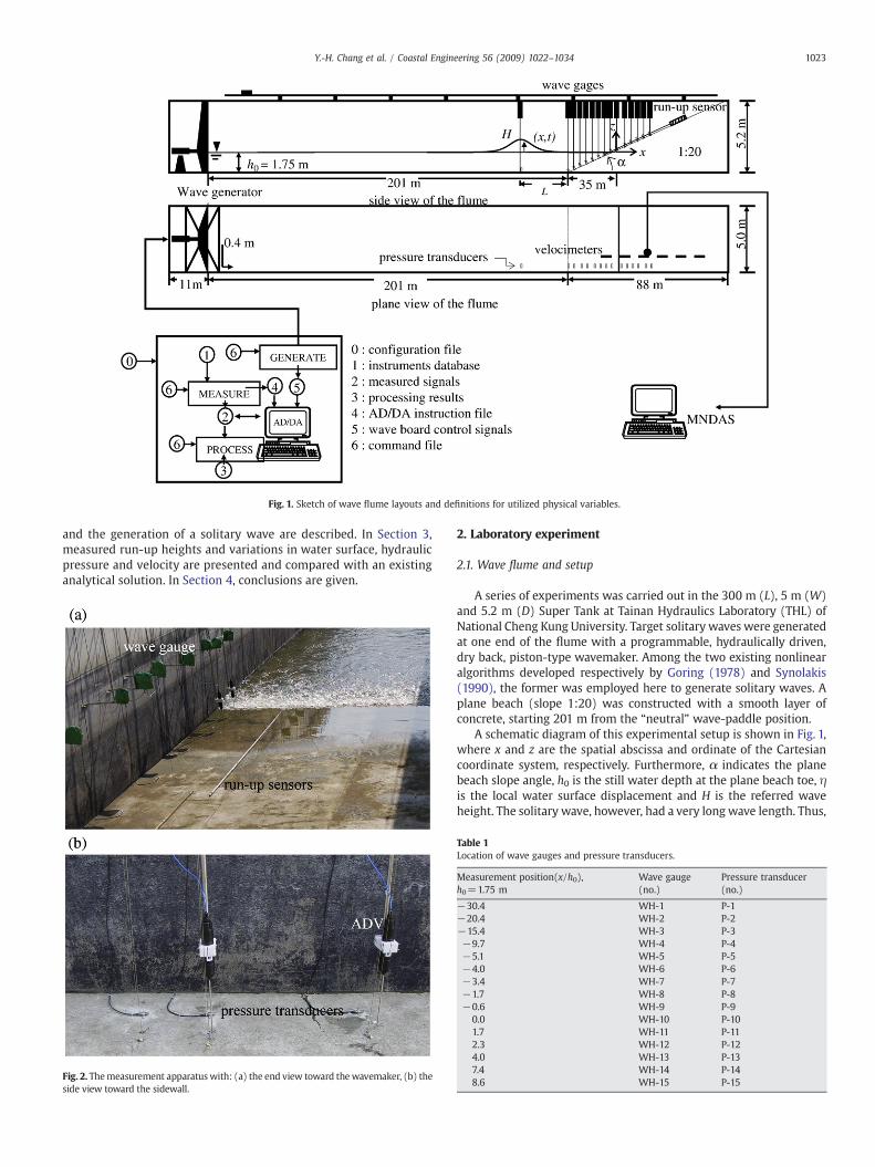
Fig. 1. Sketch of wave flume layouts and definitions for utilized physical variables.

1023Y.-H. Chang et al. / Coastal Engineering 56 (2009) 1022–1034

and the generation of a solitary wave are described. In Section 3,measured run-up heights and variations in water surface, hydraulicpressure and velocity are presented and compared with an existinganalytical solution. In Section 4, conclusions are given.

Fig. 2. Themeasurement apparatuswith: (a) the end view toward thewavemaker, (b) theside view toward the sidewall.

2. Laboratory experiment

2.1. Wave flume and setup

A series of experiments was carried out in the 300 m (L), 5 m (W)and 5.2 m (D) Super Tank at Tainan Hydraulics Laboratory (THL) ofNational Cheng Kung University. Target solitary waves were generatedat one end of the flume with a programmable, hydraulically driven,dry back, piston-type wavemaker. Among the two existing nonlinearalgorithms developed respectively by Goring (1978) and Synolakis(1990), the former was employed here to generate solitary waves. Aplane beach (slope 1:20) was constructed with a smooth layer ofconcrete, starting 201 m from the “neutral” wave-paddle position.

A schematic diagram of this experimental setup is shown in Fig. 1,where x and z are the spatial abscissa and ordinate of the Cartesiancoordinate system, respectively. Furthermore, α indicates the planebeach slope angle, h0 is the still water depth at the plane beach toe, ηis the local water surface displacement and H is the referred waveheight. The solitary wave, however, had a very long wave length. Thus,

Table 1Location of wave gauges and pressure transducers.

Measurement position(x/h0),h0=1.75 m

Wave gauge(no.)

Pressure transducer(no.)

−30.4 WH-1 P-1−20.4 WH-2 P-2−15.4 WH-3 P-3−9.7 WH-4 P-4−5.1 WH-5 P-5−4.0 WH-6 P-6−3.4 WH-7 P-7−1.7 WH-8 P-8−0.6 WH-9 P-9

0.0 WH-10 P-101.7 WH-11 P-112.3 WH-12 P-124.0 WH-13 P-137.4 WH-14 P-148.6 WH-15 P-15

Fig. 3. Set up of run-up sensors.

Table 2Location of velocimetry sensors and measurement positions.

Section Position Vertical position of velocity sensor (z/h0)(x/h0) EMV1 EMV2 EMV3 ADV1 ADV2 ADV3 ADV4

1 −4.3 −0.10 −0.15 −0.20 0.00 −0.04 – –

2 −4.0 −0.13 −0.18 – 0.00 −0.07 – –

3 −3.7 −0.08 −0.13 −0.17 0.00 −0.04 – –

4 −3.4 −0.07 −0.10 −0.13 0.13 0.00 – –

5 −2.8 −0.06 −0.09 −0.12 0.00 −0.03 – –

6 −2.2 −0.04 −0.06 −0.09 0.00 −0.02 – –

7 −0.6 – – – – – 0.02 0.008 −0.3 – – – – – 0.02 0.009 0.0 – – – – – 0.02 0.00210 0.3 – – – – – 0.04 0.0211 0.6 – – – – – 0.05 0.0312 0.9 – – – – – 0.07 0.0413 1.1 – – – – – 0.08 0.0614 1.4 – – – – – 0.10 0.0715 1.7 – – – – – 0.11 0.0816 2.0 – – – – – 0.12 0.1017 2.3 – – – – – 0.13 0.11

1024 Y.-H. Chang et al. / Coastal Engineering 56 (2009) 1022–1034

the reference gauge was installed ahead of the sloping bottom with afinite distance of L, which is the horizontal distance from solitary wavecrest to a point where the amplitude is 5% of the wave height, assuggested by Synolakis (1986).

Fig. 2 shows a photograph of the measurement facilities. Theseinclude the wave gauges, run-up sensors, pressure transducers andvelocimeters. First, elevation of the local water surface was recordedby employing 15 capacitance-type wave gauges located between182.8 m and 249.3 m downstream of the wavemaker, as detailed inTable 1. The wave gauge located at x/h0=−30.4 was the referencegauge in all tests. Each gauge was mounted 0.4 m away from thesidewall, and its response linearity was given by a high goodness-of-fitof 0.9999 (Hwung and Chiang, 2005). Among these wave gauges, fivewere located beyond the initial shoreline; these were entirely out ofthe water prior to a wave passing by, their outputs were carefullyexamined to avoid incorrect signals.

The shoreline motion was measured by run-up sensors. As the up-rush zone of this experiment stretched over 17 m, four 5 m long run-up sensors (Fig. 3) were used. The lower end of the first sensor wasinstalled at 15.2 cm under the still water level (SWL) and the otherthree were positioned lengthwise, installed at 13.5, 42.8, and 66.9 cmabove the SWL on the sloping bottom. Each run-up wire was placed ina parallel orientation, with a fixed distance of 1 cm above the bottom.With these gauges, maximum run-up height measurements can becompared to direct visual observations.

Fig. 4. Measurement positions of velocimeters.

In addition to “static” pressure, flow exerts additional dynamicpressure on surfaces perpendicular to the flow direction. Thus atransducer facing the flow direction can measure the sum of static anddynamic pressures. In the present experiments, hydraulic pressures nearthe sloping bottom were measured by using 15 pressure transducers(Druck, PDCR-1830). Each transducerhad a facediameterof 17.5mmandwas installed on the plane beach at the same horizontal locations of eachcorresponding wave gauge. All transducers were fixed with surfacesperpendicular to the sloping bottom. In the resulting sum of “static” anddynamic pressures, the static component originated from awave profilepassing by. Subtracting surface displacement from total pressure head,the remainder indicates the inherent dynamic pressure head.

For swash zone velocity measurements, in the thin, aerated andhighly dynamic environment of a swash flow, two major difficultiesare usually encountered. The first challenge is the normally very thinlayer of the run-up flow, especially with experiments at smaller scale.Another difficulty arises from entrained air bubbles produced duringthe breaking process, which always confuse velocimeters. To copewith these problems, we used a large-scale flume to enable the usageof velocimeters in thicker run-up flow. Fig. 4 shows measurementpoints of velocimeters. In surf zone, three electromagnetic veloci-meters (EMV, ALEC ACM250-A) and two down-looking probes ofacoustic Doppler velocimeters (ADV, SONTECH 16 MHz) wereemployed to measure particle velocity components at five different

Fig. 5. A generated solitary wave in the super tank.

Table 3Test conditions.

H/h0 h0 (m) cot α R (m)

0.054 1.75 20 0.3500.094 1.75 20 0.5550.164 1.75 20 0.7000.173 1.75 20 0.7400.220 1.75 20 0.8050.235 1.75 20 0.860

Fig. 7. Wave profiles of generated solitary wave with water depth h0=1.75 m. Presentexperimental data (○), the first-order theory of Grimshaw (1971) (solid line).


levels simultaneously. The EMVwas able tomeasure two components,while the ADV could measure three. The ADV can be exposed to airand was mounted transversely to the flume to minimize possiblewake effects caused by the sensor body. But for locations near or abovethe original shoreline, two side-looking probes of ADV (Nortek andVectrino) were used to measure the velocity as close to the bottom aspossible [see subplot (b) in Fig. 2]. At nine different locations withinrun-up zone (x≧0), these two ADVs were installed zb=0.5 cm andzb=5 cm above the bottom, respectively. The zb is defined here as theposition of velocimeter to the local bottom. For all tests, the accuracyof all velocimeters was 2.5 cm/s. As the velocimeters were not enoughto measure sampling points in one test run, it was necessary to repeatthe tests. Sensors were moved from one location to another andsignals were referred to the wave gauges, which were located at fixedplaces for all test runs. The measuring points are listed in Table 2.

In this large laboratory, signal synchronization from numerousparallel inputs and signal decay due to the long-distance transmissionwere two important data-acquisition problems. To cope with thesechallenges,measuring data andwave-paddlemotionwere all recordedsimultaneously with 50 Hz sampling for 400 s using a Multi-Nodes-

Fig. 6. Wave-board motion for different wave conditions with water depth h0=1.75 m.Present experimental data (○), results of Goring's (1978) method (solid line).

Data-Acquisition-System (MNDAS), developed by THL. And theanalog/digital convector used in this data-acquisition system is 12 bits.

2.2. Solitary wave generation and test conditions

Fig. 5 shows a typical solitary wave propagation in the Super Tank.The solitary wave was generated by moving the piston using Goring's(1978) method. The wavemaker was supplied designed for therequirement with a maximum stroke limit of 2 m and a maximummoving velocity limit of 1 m/s. In the present experiments, a total of 6height to depth ratios were examined as listed in Table 3, where alsolisted were their associated vertical run-up height (R). Relative waveheights (H/h0) ranged between 0.054 and 0.235,with an identicalwater

Fig. 8. Shoreline motion for a solitary wave test (H/h0=0.235, h0=1.75 m and cotα=20). The dotted line indicates time t

ffiffiffiffiffiffiffiffiffiffiffiffiffiffiffiffig = h0ð Þ

p= 1.

Fig. 9. Comparison of the normalized maximum run-up of solitary waves climbing up a1:20 beach versus normalized wave height.


depth of 1.75 m in the constant-depth region. Run-up heights were allvisually estimated of the maximum horizontal shoreline motionexcursion (ℓ) by a trigonometric expression, R=ℓ tan α. These run-up heights agreed satisfactorily with results from the run-up sensors.

Fig. 6 shows thatmeasuredwave-board trajectories of several trialsand computational results of Goring's (1978) method are in good

Fig. 10. Time histories of normalized bottom wave pressure and non-dimensional free surfpressure head (solid line); non-dimensional wave profile (-○-).

agreement, suggesting that the wavemaker is highly reliable. Themeasured offshore solitary wave profiles also agreed well with thefirst-order theory of Grimshaw (1971) as shown in Fig. 7. The abscissais a non-dimensional time variable t

ffiffiffiffiffiffiffiffiffiffiffiffiffiffiffiffig = h0ð Þp

, as adopted by Synolakis(1986). The ordinate is the wave profile, normalized with the offshoreconstant water depth, η/h0. Comparisons show that these large-scalefacilities validate the control of solitary wave generation.

3. Results and discussion

3.1. Wave run-up

Fig. 8 shows a typical shoreline motion with H/h0=0.235, ofwhich time histories were assembled from four run-up sensors. Themaximum run-up occurred at t


p e24:9, while the maximumexcursion x/h0=9.7, with x=16.9 m. This is close to the directobservation of maximum shoreline motion excursion (ℓ=17.2 m).Considering the gap between run-up wires and the sloping bottom,these visually determined maximum run-up excursions agreedreasonably well with the detected run-up motions. Using a two-point central difference, the initial run-up velocity at approximatelyt


p= 0 was found to be 1.7 m/s. However, the velocity

immediately after tffiffiffiffiffiffiffiffiffiffiffiffiffiffiffiffig = h0ð Þ

p= 1 was found to rapidly increase to

about 5.7 m/s. It appears that there was a fluid acceleration in theearly stages of run-up. This has been noted by Synolakis (1986) anddiscussed by Synolakis and Bernard (2006).

ace displacement for a solitary wave (H/h0=0.235, h0=1.75 m and cot α=20). Total

Fig. 11. The spatial distribution of maximum wave pressure for various solitary waveconditions.

Fig. 13. Flow measurements in the thin, aerated swash zone.


Fig. 9 compares the present large-scale laboratory data withexisting estimations of maximum run-up height. Synolakis (1986)proposed an empirical expression for breaking solitary wavesclimbing up a 1:20 slope. The expression was described as R/h0=1.109 (H/h0)0.582 in which the determination of run-up height wasbased on the maximum position of the shoreline. For the run-up onvarious plane bottoms of slope, Li and Raichlen (2003) developed anempirical method by employing the energy balance model (EBM).Based on the nonlinear least-square algorithm, Hsiao et al. (2008)proposed another empirical expression, R/h0=7.712(cot α)−0.632

(sin (H/h0)) 0.618. Overall, the three empirical expressions can wellcapture the run-up heights for breaking solitary waves climbingupon a 1:20 slope. Both the estimations of Synolakis (1986) andHsiao et al. (2008) are slightly smaller than present laboratory data.The empirical expression of Li and Raichlen (2003) predictsapparently lower than the present laboratory data, but it worksbetter as H/h0N0.175.

3.2. Wave propagation and pressure evolution

Fig. 10 shows a typical pressure evolution as a solitary wavepropagates onshore. It presents time histories of the bottom wavepressure and free surface fluctuations along the wave flume with H/h0=0.235. The ordinate is the total pressure head, normalized with

Fig.12. The spatial distribution of hydrodynamic pressure with respect to themaximumwave pressure.

offshore wave height, p/ρgH; and it also denotes the ratio η/H. Inaddition to a non-dimensional surface profile, the ratio η/H is thenon-dimensional “static” pressure of a wave passing by.

Fig. 11 gives the distribution of normalized maximum wavepressure distributions (pmax/ρgH) along the wave flume. Symbolsdenote experimental data under different wave conditions. In order toplot swash pressure evolutions in the same dimensionless scale, themaximum run-up excursion ℓ of each test was employed as thecharacteristic length scale for normalization. For all tests, thedimensionless run-up zone is thus ranged between x/ℓ=0 andx/ℓ=1. With the same spatial abscissa, Fig. 12 further presentsthe inherent hydrodynamic component in pd=p−ρgη, and ηpmax isvalue of the free surface at the occurrence of maximum pressure pmax.

From Figs. 11 and 12, the entire pressure evolution for the test withH/h0=0.235 (Fig. 10) can be divided into three stages by theoccurrence of wave breaking and run-up. Initially, the wave heightgradually increased as the generated solitary wave propagated ontothe sloping bottom. The front face became steeper until it reached itsmaximum at the breaking point (x/h0=−3.14), and the wave sloweddown as it propagated into the sloping bottom (Synolakis andSkjelbreia, 1993; Hwang et al., 2007). Near the breaking point, thesurface elevation exhibited a narrow peak at the leading edgefollowed by an extended, triangular wedge-shaped region. A similarprofile pattern was observed in the evolution of wave pressure.Clearly, the principal bottom wave pressure before breaking arosefrom the “static” pressure of the wave profile because if one uses somecriteria the variance of the pressure fall the “hydrostatic” value ρgη.Meanwhile, the solitary wave also increases in dynamic pressure, butits growth is not apparent as that in “hydrostatic” component.

In the second stage, the wave front turned into a turbulent boreand maintained approximately an extended wedge-shape afterbreaking. Subsequently, this bore propagated toward the shorelineand eventually climbed onto the beach. The problem of borepropagation over a sloping sea-floor was approximated using thesolutions of nonlinear shallow-water equations, as given byWhitham (1958). While approaching the shoreline, the predictedbore height tends to vanish. Also, the fluid and front velocitiesapproach their common finite value, but their acceleration becomessingular. Yeh et al. (1989) demonstrated that the acceleration inbore-collapse is caused by a ‘momentum exchange’ process ratherthan amathematical singularity, as described in shallow-water wavetheory. The ‘momentum exchange’ process is the interactionbetween a bore and the initially quiescent water along a shoreline.Overall, the “static” pressure decreased with the amplitude evolu-tion of a breaking solitary wave in the zones of rapid and gradual

Fig. 14. Snapshots of measured particle velocities and measured surface elevations for the solitary wave (H/h0=0.235, h0=1.75 m and cot α=20).


Fig. 14 (continued).

Fig. 15. Definition sketch of Peregrine and Williams (2001).


decay, as suggested by Synolakis and Skjelbreia (1993). Meanwhile,the hydrodynamic pressure was firstly attenuated at x/h0=−3.4[i.e. x/ℓ=−0.34] which is near the breaking point (x/h0=−3.14).On the contrary, the subsequent growth of total pressure indicatesthat the first gradual increase of hydrodynamic pressure was atx/h0=−1.7 [i.e. x/ℓ=−0.17]. This then rapidly increased, owing toa bore-collapse that caused the rapid conversion of potential energyinto kinetic energy.

In the third stage, the bore begins climbing onto the plane beach.The whole sheet of run-up flow becomes thinner as time increases,but the run-up tip at first keeps the previous stage state, withacceleratedmotion. Therefore, the total pressure is still growing untilx/h0=2.3, where the wave pressure reaches its maximumvalue andsimultaneous deceleration commences. When x/h0N2.3, the motionis dominated by gravity and ultimately retarded by bottom shearstress.

For the other wave conditions, the pressure evolutions are alsodisplayed in Figs. 11and12. Most importantly, Figs. 11 and 12 showthat large pressures are concentrated in the leading 1/4 run-up zone,0bx/ℓb1/4, in which hydrodynamic pressure is the principalcomponent. Among these large pressures, the ratio of hydrodynamicto total pressure reaches 75–99%, and the maximum hydrodynamicpressure head approaches five times the initial solitary wave height.

3.3. Velocity measurements of run-up flow

Fig. 13 shows the difficulty of velocity measurements encounteredin the thin, aerated swash zone, where the solid line denotes thehorizontal velocity measured at the still shoreline (x/h0=0, z/h0=0.002). The water surface at the same horizontal position is alsoplotted for comparing the two measurements. Significant spikeswere observed, originating from the highly turbulent and/or aeratedflow of the run-up tongue passing themeasuring volume. The velocitysignal fluctuated widely around a zero mean. This acoustic scatteringwas excluded from further analyses. Hence, the apparent localacceleration of the run-up tip cannot be observed in the remainingavailable data.

Despite difficulties in measuring the post-breaking and the thinaerated swash flow, the available data are helpful for studying the flowbehind the run-up tongue. Fig. 14 provides eight snapshots of the

measured velocity vector and free surface as a solitary wave propagatedonshore, where V =

ffiffiffiffiffiffiffiffiffiffiffiffigh0ð Þp

is the velocity vector with a normalizationof the shallow-water wave celerity

ffiffiffiffiffiffiffiffiffiffiffiffigh0ð Þ

ph i. Measurement positions

of velocimeters can be referred to Fig. 4 and Table 2. The testingconditions were: H/h0=0.235, h0=1.75 m and cot α=20. Fig. 14(a)shows the moment shortly after the occurrence of plunging breaker.The flow behind the wave front appears uniform, while approachingwave front it becomes more random due to plunging breaker. Fig. 14(b)shows the instant that the bore is about to be climbing up the slope.Panels (c)–(d) of Fig. 14 show the initial run-up motion stage. Twosubsequent snapshots are depicted in Fig. 14(e)–(f), where the particlevelocities decrease from the run-up front towards the still shoreline assimulated by Lin et al. (1999). An interesting phenomenawas observedin Fig. 14(g): at t


p= 14:3, the flow runs in opposite directions:

in the upper region (x/h0N1.0) the flow keeps going onshore, while inthe lower region (x/h0b1.0) the flow has begun to retreat offshore.Similar phenomena can also be seen in Fig. 14(h), and the flow inx/h0b2.3 is all retreating. However, at this moment, t


p= 19:1,

the run-up tip should be still climbing up the beach since themaximumrun-up occurs at t


p e24:9, as shown in Fig. 8 (Section 3.1).

3.4. Comparison of theoretical and experimental run-up flow

An analytical solution based on the nonlinear shallow-waterequations for uniform sloping bottoms was developed by Shen andMeyer (1963) for the run-up of an incident bore. The solutionindicates that, at the run-up tip, the water surface is tangential to thebed. In the nonlinear shallow-water equations, some real conditionssuch as bed roughness and viscosity are neglected for simplifying the

Fig. 16. Comparison of the analytical water thickness to the present laboratory data at different locations. Wave condition: H/h0=0.235, h0=1.75 m and cot α=20. PW (2001), i.e.Eq. (2) (solid line); present experimental data (-○-).


inherent complication. Nonetheless, Peregrine and Williams (2001)showed that the solution is a good approximation to wave motion inthe swash zone.

Peregrine andWilliams (2001) provided an equation for temporaland spatial variations in flow velocity. The associated definitionsketch is shown in Fig. 15, where x⁎1 is measured up the slope, h⁎1 is thewater thickness of flow, u⁎1 is the water velocity parallel to the beachand the vertical excursion of the maximum run-up height is denotedas 2A [i.e. 2A=R], t is counted from the instant the run-up frontbegins to climb up the sloping beach. These physical variables arefurther converted into dimensionless variables by x1=x⁎1 sin α/A,t1= t sin α

ffiffiffiffiffiffiffiffiffiffig = A

p, h1=h⁎1 cos α/A, and u1=u⁎1/

ffiffiffiffiffiffigA

p. As mentioned

by Shen and Meyer (1963), the flow of the run-up tip moves up anddown the beach under gravity, just like a freely moving particle. Thedimensionless shoreline motion is then described by:

xs t1ð Þ = 2t1 − 12t21 : ð1Þ

While at t1=2, the run-up tip reaches the maximum run-upheight (2A) at xs=2, and simultaneously begins to run-down thebeach. That is, the run-up tip passes the position of x1 at

t1 = 2−ffiffiffiffiffiffiffiffiffiffiffiffiffiffiffiffiffiffiffiffiffi4− 2x1ð Þp

and 2 +ffiffiffiffiffiffiffiffiffiffiffiffiffiffiffiffiffiffiffiffiffi4− 2x1ð Þp

during the run-up andrun-down, respectively. In Shen and Meyer (1963), the water depthlocal to the shoreline which was a dimensional variable defined in aCartesian coordinate system. It can be transformed into a dimensionlesswater thickness defined in the (x1, t1) plane, as given by Peregrine andWilliams (2001):

h1 x1; t1ð Þ = 19t21

xs t1ð Þ−x1ð Þ2 =1

36t214t1−t21−2x1

� �2; t1 N 0: ð2Þ

Meanwhile, the flow velocity in the run-up phasewas described byPeregrine and Williams (2001):

u1 x1; t1ð Þ = 23t1

t1 − t21 + x1� �

: ð3Þ

The analytical flow velocity at the tip (x1=xs) is equal to the tipvelocity by differentiating Eq. (1) with respect to t1. In other words,the tip velocity us is

us t1ð Þ = 2− t1: ð4Þ

Fig. 17. Comparison of the analytical flow velocity to the present laboratory data at different locations. Wave condition: H/h0=0.235, h0=1.75 m and cot α=20. PW (2001), i.e. Eq.(3) (solid line); the ADV at zb=0.5 cm (○); the ADV at zb=5.0 cm (×).


To comparewith the analytical solution of Peregrine andWilliams(2001), the present measurements of water depth and flow velocitywere all transformed into dimensionless forms in the (x1, t1) plane.Fig. 16 shows comparisons of the present laboratory water thickness

and the analytical prediction of Peregrine and Williams (2001), i.e.Eq. (2), where the computation of Peregrine and Williams (2001) isabbreviated as PW (2001). The test conditions are: H/h0=0.235,h0=1.75 m and cot α=20. From each subplot of different locations,

Fig. 18. Calibration of the drag coefficient (CD=1.2) at different locations. Wavecondition: H/h0=0.235, h0=1.75 m and cot α=20. Eq. (6) (○); present experimentaldata (solid line).


the whole sheet of run-up flow becomes thinner as time increases.Clearly, comparisons show that the analytical solution underesti-mates the actual water depth.

Fig.17 gives comparisons between the present laboratory data andthe PW (2001) flow velocity at different locations. In each subplot,symbols are two records measured at different levels: zb=0.5 cmand 5 cm above the local bottom. The valid data for the ADV installedat zb=0.5 cm was much more than that installed at zb=5 cm,because the lower the measuring point the longer it stayed in water.The flow velocities at zb=5 cm are slightly larger than thosemeasured at zb=0.5 cm. Clearly, the vertical distribution of flowvelocity in the up-rush was more uniform than during the down-rush, as discussed by Elfrink and Baldock (2002) and Cowen et al.(2003).When comparing flowvelocities between the laboratory dataand the solution of PW (2001) [i.e. Eq. (3)], the velocity equation is areasonable approximation for describing the flow evolution atdifferent locations during the run-up process.

3.5. Estimation of the maximum hydrodynamic pressure in the up-rush zone

The resultant dynamic force (i.e., drag force or the resistance tomotion) exerted on an immersed body in steady flowcan be computedby:

Fd =12ρCDBh41u4

21 ; ð5Þ

where ρ is the fluid density, B is the breadth of the immersed body inthe plane normal to the flow direction, and CD is the drag coefficient

depending on the width-to-depth ratio. The term (h⁎1 u⁎12) gives the

momentum flux per-unit-mass per-unit-breadth. Dividing through bythe frontal area normal to the run-up flow (Bh⁎1), the meanhydrodynamic pressure over the area is:

Pd =12ρCD u41

� �2: ð6Þ

The drag coefficient can be evaluated by the synchronous validsignal of velocity and pressure in the present experiment. Fig. 18shows the fit between experiment and prediction for a drag coefficientof CD=1.2. Note that the hydrodynamic pressures at different stationsare expressed in dimensional units and the present calibration onlyaims to record the onshore phase. Thus the hydrodynamic pressuresexerted on circular pressure transducers can be evaluated by Eq. (6)with CD=1.2, even for this unsteady flow.

Applying the analytical flow velocity of PW (2001), i.e. Eq. (3) toEq. (6), the simulation presented here provides reasonable hydro-dynamic pressures in comparison with laboratory data, as shown inFig. 19. Note that pd/ρgR is the hydrodynamic pressure, with anormalization of the pressure head with maximum run-up heightsover the entire flow. As a result of the gravity-governed motion inShen and Meyer (1963), the analytical solution of PW (2001) cannotdescribe the acceleration observed in the initial run-up motion stage.That is, the present simulation of hydrodynamic pressure alsounderestimates the impact of solitary wave by using the sameanalytical solution of flow velocity.

Evidently, surging is highly transient andnotwell understood. Fig. 20presents the normalized maximum hydrodynamic pressure distribu-tions (pd/ρgR)max for different solitary wave tests. The predictedmaximum hydrodynamic pressures of Eq. (6) with different dragcoefficients are alsoplotted together. Themaximumfluid velocity occursat the leading run-up tip. Using the dimensional form of the tip velocityus

ffiffiffiffiffiffiffiffiffiffigAð Þp

in Eq. (6), the maximum hydrodynamic pressure can beevaluated as:

pdð Þmax =12ρCD us

ffiffiffiffiffiffigA

p� �2: ð7Þ

A closely related quantity is stress by dividing through ρg2A andsubstituting the dimensionless tip velocity by Eq. (4), which relatesthe maximum hydrodynamic pressure (Pd)max to the dimensionlesstime, t1, via:

pdρg2A

� �max

= CDu2s

4=

CD

42−t1ð Þ2: ð8Þ

After substitution of the expression R=2A and the relationship oftime to the tip position during run-up phase, t1 = 2−

ffiffiffiffiffiffiffiffiffiffiffiffiffiffiffiffiffiffiffiffiffi4− 2x1ð Þp

,this lead to:

pdρgR

� �max

= CD 1− 0:5x1ð Þ: ð9Þ

With the previously determined drag coefficient CD=1.2, thecomputation of Eq. (9) is given as a solid line in Fig. 20. While theflow is in the upper run-up zone (x1N1.0) it becomes slow and can becharacterized as quasi-steady. Thus, the predictions agree well with thelaboratory data. In contrast, this prediction underestimates actualmaximum hydrodynamic pressures in the leading 1/4 run-up zonewith a CD=1.2. In line with the suggestion of Yeh (2007), the designhydrodynamic pressure can be estimated with a higher drag coefficient

Fig. 19. Comparison of the predicted hydrodynamic pressures to the present laboratory data at different locations. Wave condition: H/h0=0.235, h0=1.75 m and cot α=20. Eq. (6)(solid line); present experimental data (○).


for conservatism. As the dashed line indicates, the result of CD=2.4 isclose to the maximum measured hydrodynamic pressures.

4. Conclusions

In this study, a series of laboratory experiments for breakingsolitary waves on a 1:20 uniform slope was carried out with relativewave heights H/h0 ranged between 0.054 and 0.235 in a 300 m supertank. Laboratory results, including detailed particle velocities andpressures, are presented and compared to one available analytical

Fig. 20. Distribution of maximum hydrodynamic pressure in run-up zone.

solution for the run-up flow. The present laboratory data of run-upheights is also compared with the existing estimations for breakingsolitary waves climbing up a 1:20 slope.

Although themotion of a freelymoving particle and correspondingsimplified conditions do not accurately represent a real run-up flow,the analytical solution of Peregrine and Williams (2001) [i.e. Eq. (3)]provides a convenient prediction of the run-up flow velocity. Throughcalibration of the drag coefficient, the analytical flow velocity appearsreasonable for the prediction of hydrodynamic pressure.

Most importantly, large pressures were concentrated in theleading 1/4 run-up zone. The dynamic pressure is the principalcomponent of this large pressure and its maximum pressure headapproached five times the initial solitary wave height. For the extrapressure, which is evidently exerted upon impact of the leading waveedge, the design hydrodynamic pressure must be computed with itsapproximate drag coefficient. As an example of the present study, thedesign hydrodynamic pressure for a circular pressure transducer wasestimated with a CD=2.4 instead of 1.2, especially in the lead up tothe run-up zone.

Acknowledgments

The authors would like to express sincere gratitude to the “NCKUProject of Promoting Academic Excellence & Developing World ClassResearch Centers”, which was supported by the Ministry of Education,Taiwan. In addition, many thanks are due to the Senior DesignEngineer, Lambert N.G. Romijnders Development & Control of BoschRexroth B.V., and the research staff of Tainan Hydraulics Laboratory forperforming a series of experiments.


References

Cowen, E.A., Sou, I.M., Liu, P.L.-F., Raubenheimer, B., 2003. Particle image velocimetrymeasurements within a laboratory-generated swash zone. J. Engrg. Mech. 129,1119–1129.

Elfrink, B., Baldock, T., 2002. Hydrodynamics and sediment transport in the swash zone:a review and perspective. Coast. Eng. 45, 149–167.

Geist, E.L., Titov, V.V., Synolakis, C.E., 2006. Tsunami: wave of change. Sci. Am. 294,56–63.

Goring, D.G., 1978. Tsunami: the propagation of long waves on a shelf. Report KH-R-38.M. Keck Laboratory of Hydraulics and Water Resources. California Institute ofTechnology, Pasadena, CA.

Grilli, S.T., Svendsen, I.A., Subramanya, R., 1997. Breaking criterion and characteristics forsolitary waves on slopes. J. Wtrwy., Port, Coast. Oc. Engrg. 123, 102–112.

Grimshaw, R., 1971. The solitary wave in water of variable depth. J. Fluid Mech., 46,611–622.

Hsiao, S.-C., Hsu, T.-W., Lin, T.-C., Chang, Y.-H., 2008. On the evolution and run-up ofbreaking solitarywaves on amild sloping beach. Coast. Eng. 55, 975–988. doi:10.1016/j.coastaleng.2008.03.002.

Hwang, K.-S., Chang, Y.-H., Hwung, H.-H., Li, Y.-S., 2007. Large scale experiments onevolution and run-up of breaking solitary waves. J. Earthqu. Tsunami 1, 257–272.

Hwung, H.H., Hwang, K.S., Chiang, W.S., Lai, C.F., 1998. Flow structures in swash zone.26th International Conference on Coastal Engineering. ASCE, pp. 2826–2836.

Hwung, H.H., Chiang, W.S., 2005. Measurements of wave modulation and breaking.Meas. Sci. Technol. 16, 1921–1928.

Jensen, A., Pederson, G.K., Wood, D.J., 2003. An experimental study of wave run-up at asteep beach. J. Fluid Mech. 486, 161–188.

Li, Y., Raichlen, F., 2001. Solitary wave runup on plane slopes. J. Wtrwy., Port, Coast. andOc. Engrg. 127, 33–44.

Li, Y., Raichlen, F., 2002. Non-breaking and breaking solitary wave run-up. J. Fluid Mech.456, 295–318.

Li, Y., Raichlen, F., 2003. Energy balance model for breaking solitary wave run-up. J.Waterway, Port, Coastal, Ocean Eng. 129, 47–59.

Lin, P., Chang, K.A., Liu, P.L.-F., 1999. Runup and rundown of solitary waves on slopingbeaches. J. Waterway, Port, Coastal, Ocean Eng. 125, 247–255.

O'Donoghue, T., Hondebrink, L.J., Pokrajac, D., 2006. Bore-driven swash on beaches:numerical modeling and large-scale laboratory experiments. 30th InternationalConference on Coastal Engineering. ASCE, pp. 922–933.

Peregrine, D.H., Williams, S.M., 2001. Swash overtopping a truncated plane beach. J.Fluid Mech. 440, 391–399.

Robertson, I., Riggs, H.R., Yim, S.C., Young, Y.L., 2007. Lessons from Hurricane Katrinastorm surge on bridges and buildings. J. Wtrwy., Port, Coast. Oc. Engrg. 133 (6),463–483.

Shen, M.C., Meyer, R.E., 1963. Climb of a bore on a beach, Part 3, Run-up. J. FluidMech.16,113–125.

Synolakis, C.E., 1986. The runup of long waves. Ph. D. Thesis, California Institute ofTechnology, Pasadena, California, 228pp.

Synolakis, C.E., 1987. The runup of solitary waves. J. Fluid Mech. 185, 523–545.Synolakis, C.E., 1990. On the generation of long waves in the laboratory. J. Wtrwy., Port,

Coast. Oc. Engrg., ASCE 116 (2), 252–266.Synolakis, C.E., 2003. Tsunami and seiche. In: Chen, W.F., Scawthorn, C. (Eds.),

Earthquake Engineering Handbook. CRC Press, p. 9. 1 to 9-90.Synolakis, C.E., Bernard, E.N., 2006. Tsunami science before and after Boxing Day 2004.

Philos. Trans., A 364, 2231–2265. doi:10.1098/rsta.2006.1824.Synolakis, C.E., Skjelbreia, J.E., 1993. Evolution of maximum amplitude of solitary waves

on plane beaches. J. Wtrwy. Port, Coast. Oc. Engrg. 119 (3), 323–342.Ting, F.C.K., 2006. Large-scale turbulence under a solitary wave. Coast. Eng. 53, 441–462.Whitham, G.B., 1958. On the propagation of shock waves through regions of non-

uniform area of flow. J. Fluid Mech. 4, 337–360.Yeh, H., 2007. Design Tsunami forces for onshore structures. J. Disaster Res. 2, 531–536.Yeh, H., Ghazali, A., Marton, I., 1989. Experimental study of bore run-up. J. Fluid Mech.

206, 563–578.

Documents

Large-scale laboratory measurements of solitary wave inundation on a 1:20 slope