Embed Size (px)
Citation preview

Large Scale computation of Means and Clusters forPersistence Diagrams using Optimal Transport
Théo LacombeDatashape
Inria [email protected]
Marco CuturiCRESTENSAE
Steve OudotDatashape
Inria [email protected]
Abstract
Persistence diagrams (PDs) are now routinely used to summarize the underlyingtopology of sophisticated data encountered in challenging learning problems. De-spite several appealing properties, integrating PDs in learning pipelines can bechallenging because their natural geometry is not Hilbertian. In particular, algo-rithms to average a family of PDs have only been considered recently and areknown to be computationally prohibitive. We propose in this article a tractableframework to carry out fundamental tasks on PDs, namely evaluating distances,computing barycenters and carrying out clustering. This framework builds upon aformulation of PD metrics as optimal transport (OT) problems, for which recentcomputational advances, in particular entropic regularization and its convolutionalformulation on regular grids, can all be leveraged to provide efficient and (GPU)scalable computations. We demonstrate the efficiency of our approach by carryingout clustering on PDs at scales never seen before in the literature.
1 IntroductionTopological data analysis (TDA) has been used successfully in a wide array of applications, forinstance in medical (Nicolau et al., 2011) or material (Hiraoka et al., 2016) sciences, computervision (Li et al., 2014) or to classify NBA players (Lum et al., 2013). The goal of TDA is to exploitand account for the complex topology (connectivity, loops, holes, etc.) seen in modern data. Thetools developed in TDA are built upon persistent homology theory (Edelsbrunner & Harer, 2010)whose main output is a descriptor called a persistence diagram (PD) which encodes in a compactform—roughly speaking, a point cloud in the upper triangle of the square [0, 1]2—the topology of agiven space or object at all scales.
Statistics on PD. Persistence diagrams have appealing properties: in particular they have been shownto be stable with respect to perturbations of the input data (Cohen-Steiner et al., 2007; Chazal et al.,2009, 2014). This stability is measured either in the so called bottleneck metric or in the p-th diagramdistance, which are both distances that compute optimal partial matchings. While theoreticallymotivated and intuitive, these metrics are by definition very costly to compute. Furthermore, thesemetrics are not Hilbertian, preventing a faithful application of a large class of standard machinelearning tools (k-means, PCA, SVM) on PDs.
Related work. To circumvent the non-Hilbertian nature of the space of PDs, one can of course mapdiagrams onto simple feature vectors. Such features can be either finite dimensional (Carrière et al.,2015a; Adams et al., 2017), or infinite through kernel functions (Bubenik, 2015; Carrière et al., 2017).A known drawback of kernel approaches on a rich geometric space such as that formed by PDs is thatonce PDs are mapped as feature vectors, any ensuing analysis remains in the space of such features(the “inverse image” problem inherent to kernelization). They are therefore not helpful to carry outsimple tasks in the space of PDs, such as that of averaging PDs, namely computing the Fréchet mean
Preprint. Work in progress.
arX
iv:1
805.
0833
1v1
[st
at.M
L]
22
May
201
8

of a family of PDs. Such problems call for algorithms that are able to optimize directly in the space ofPDs, and were first addressed by Mileyko et al. (2011); Turner (2013). Turner et al. (2014) providedan algorithm that converges to a local minimum of the Fréchet function by successive iterations ofthe Hungarian algorithm. However, the Hungarian algorithm does not scale well with the size ofdiagrams, and non-convexity yields potentially convergence to bad local minima.
Contributions. We reformulate the computation of diagram metrics as an optimal transport problem,opening several perspectives, among them the ability to benefit from fast entropic regularization (Cu-turi, 2013). We provide a new numerical scheme to bound OT transport metrics, and therefore diagrammetrics, with additive guarantees. Unlike previous approximations of diagram metrics, ours can beparallelized and implemented efficiently on GPUs. These approximations are also differentiable,leading to an extremely efficient method to solve the barycenter problem for persistence diagrams. Inexchange for a discretized approximation of PDs, we recover a convex problem, unlike previous PDsbarycenter formulations. We demonstrate the scalability of these two advances (accurate approxi-mation of the diagram metric at scale and barycenter computation) by providing the first tractableimplementation of the k-means algorithm in the space of persistence diagrams.
2 Background on OT and TDAOT. Optimal transport is now widely seen as a central tool to compare probability measures (Villani,2003, 2008; Santambrogio, 2015). Given a space X endowed with a cost function c : X × X → R+,we consider two discrete measures µ and ν on X , namely measures that can be written as positivecombinations of diracs, µ =
∑ni=1 aiδxi , ν =
∑mj=1 bjδyj with weight vectors a ∈ Rn+, b ∈ Rm+
verifying∑i ai =
∑j bj and all xi, yj in X . The n × m cost matrix C = (c(xi, yj))ij and the
transportation polytope Π(a, b) = {P ∈ Rn×m+ |P1m = a, PT1n = b} define an optimal transportproblem whose optimum LC can be computed using either of two linear programs, dual to each other,
LC(µ, ν) := minP∈Π(a,b)
〈P,C〉 = max(α,β)∈ΨC
〈α, a〉+ 〈β, b〉 (1)
where 〈·, ·〉 is the Frobenius dot product and ΨC is the set of pairs of vectors (α, β) in Rn×Rm suchthat their tensor sum α⊕ β is smaller than C, namely ∀i, j, αi + βj ≤ Cij . Note that when n = mand all weights a and b are uniform and equal, the problem above reduces to the computation of anoptimal matching, that is a permutation σ ∈ Sn (with a resulting optimal plan P taking the formPij = 1σ(i)=j). That problem has clear connections with diagram distances, as shown in §3.
Entropic Regularization. Solving the optimal transport problem is intractable for large data.Cuturi proposes to consider a regularized formulation of that problem using entropy h(P ) :=−∑ij Pij(logPij − 1), namely:
LγC(a, b) := minP∈Π(a,b)
〈P,C〉 − γh(P ) (2)
= maxα∈Rn,β∈Rm
〈α, a〉+ 〈β, b〉 − γ∑
i,j
eαi+βj−Ci,j
γ , (3)
where γ > 0. Because the negentropy is 1-strongly convex, that problem has a unique solution P γwhich takes the form, using first order conditions,
P γ = diag(uγ)Kdiag(vγ) ∈ Rn×m (4)
where K = e−Cγ (term-wise exponentiation), and (uγ , vγ) ∈ Rn × Rm is a fixed point of the
Sinkhorn map (term-wise divisions):
S : (u, v) 7→(
a
Kv,
b
KTu
)(5)
Cuturi considers the transport cost of the optimal regularized plan, SγC(a, b) := 〈P γ , C〉 =(uγ)T (K � C)vγ , to define a Sinkhorn divergence between a, b (here � is the elementwise product).One has that SγC(a, b) → LC(a, b) as γ → 0, and more precisely P γ converges to the optimaltransport plan solution of (1) with maximal entropy. That approximation can be readily applied toany problem that involves terms in LC , notably barycenters (Cuturi & Doucet, 2014; Solomon et al.,2015; Benamou et al., 2015).
2

Persistence diagramSublevels sets of f = distPInput data: point cloud P
Figure 1: Sketch of persistent homology. X = R3 and f(x) = minp∈P ‖x− p‖ so that sublevel sets of f areunions of balls centered at the points of P . First (resp second) coordinate of points in the persistence diagramencodes appearance scale (resp disappearance) of cavities in the sublevel sets of f . The isolated red pointaccounts for the presence of a persistent hole in the sublevel sets, inferring the underlying spherical geometry ofthe input point cloud.
Eulerian setting. When the set X is finite with cardinality d, µ and ν are entirely characterizedby their probability weights a, b ∈ Rd+ and are often called histograms in a Eulerian setting. WhenX is not discrete, as when considering the plane [0, 1]2, we therefore have a choice of representingmeasures as sums of diracs, encoding their information through locations, or as discretized histogramson a planar grid of arbitrary granularity. Because the latter setting is more effective for entropicregularization (Solomon et al., 2015), this is the approach we will favor in our computations.
Persistent homology and Persistence Diagrams. Given a topological space X and a real-valuedfunction f : X → R, persistent homology provides—under mild assumptions on f , taken forgranted in the remaining of this article—a topological signature of f built on its sublevel sets(f−1((−∞, t])
)t∈R, and called a persistence diagram (PD), denoted as Dgm(f). It is of the form
Dgm(f) =∑ni=1 δxi , namely a point measure with finite support included in R2
> := {(s, t) ∈R2|s < t}. Each point (s, t) in Dgm(f) can be understood as a topological feature (connectedcomponent, loop, hole...) which appears at scale s and disappears at scale t in the sublevel setsof f . Comparing the persistence diagrams of two functions f, g measures their difference from atopological perspective: presence of some topological features, difference in appearance scales, etc.The space of PDs is naturally endowed with a partial matching metric defined as (p ≥ 1):
dp(D1, D2) :=
minζ∈Γ(D1,D2)
∑
(x,y)∈ζ‖x− y‖pp +
∑
s∈D1∪D2\ζ‖s− π∆(s)‖pp
1p
, (6)
where Γ(D1, D2) is the set of all partial matchings between points in D1 and points in D2 and π∆(s)denotes the orthogonal projection of an (unmatched) point s to the diagonal {(x, x) ∈ R2, x ∈ R}.The mathematics of OT and diagram distances share a key idea, that of matching, but differ on animportant aspect: diagram metrics can cope, using the diagonal as a sink, with measures that have avarying total number of points. We solve this gap by leveraging an unbalanced formulation for OT.
3 Fast estimation of diagram metrics using Optimal TransportIn the following, we start by explicitely formulating (6) as an optimal transport problem. Entropicsmoothing provides us a way to approximate (6) with controllable error. In order to benefit mostlyfrom that regularization (matrix parallel execution, convolution, GPU—as showcased in (Solomonet al., 2015)), implementation requires specific attention, as described in propositions 2, 3, 4.
PD metrics as Optimal Transport. The main differences between (6) and (1) are that PDs do notgenerally have the same number of points and that the diagonal plays a special role by allowingto match any point x in a given diagram with its orthogonal projection π∆(x) onto the diagonal.Guittet’s formulation for partial transport (2002) can be used to account for this by creating a “sink”bin corresponding to that diagonal and allowing for different total masses. The idea of representingthe diagonal as a single point is also present in the bipartite graph problem of Edelsbrunner & Harer(2010) (Ch.VIII). The important aspect of the following proposition is the clarification of the partialmatching problem (6) as a standard OT problem (1).
Let R2> ∪ {∆} be R2
> extended with a unique virtual point {∆} encoding the diagonal. We introducethe linear operator R which, to a measure µ inM+(R2
>), associates a dirac on ∆ with mass equal tothe total mass of µ, namely R(µ) = |µ|δ∆.
3

Proposition 1. Let D1 =∑n1
i=1 δxi and D2 =∑n2
j=1 δyj be two persistence diagrams with respec-tively n1 points x1..xn1
and n2 points y1..yn2. Let p ≥ 1. Then:
dp(D1, D2)p = LC(D1 + RD2, D2 + RD1), (7)
where C is the cost matrix with block structure
C =
(C uvT 0
)∈ R(n1+1)×(n2+1), (8)
where ui = ‖xi − π∆(xi)‖p, vj = ‖yj − π∆(yj)‖p, Cij = ‖xi − yj‖p, for i ≤ n1, j ≤ n2.
The proof seamlessly relies on the fact that, when transporting point measures with the same numberof points, the optimal transport problem is equivalent to an optimal matching problem (see §2). Forthe sake of completeness, we provide details in the supplementary material .
Entropic approximation of diagram distances. Following the correspondance established inProp 1, entropic regularization can be used to approximate the diagram distance dp(·, ·). Giventwo persistence diagrams D1, D2 with respectively n1 and n2 points, let n := n1 + n2 and P γt =diag(uγt )Kdiag(vγt ) where (uγt , v
γt ) is the output after t iterations of the Sinkhorn map (5) starting
from an arbitrary initialization. Adapting the bounds provided by Altschuler et al. (2017), we canbound the error of approximating dp(D1, D2)p by 〈P γt , C〉:
|dp(D1, D2)p − 〈P γt , C〉 | ≤2γn log (n) + dist(P γt ,Π(a, b))‖C‖∞ (9)
where dist(P,Π(a, b)) := ‖P1− a‖1 + ‖PT1− b‖1 (that is, error on marginals).
In recent work of Dvurechensky et al. (2018), authors prove that iterating the Sinkhorn map (5) givesa plan P γt verifying dist(P γt ,Π(a, b)) < ε in O
(‖C‖2∞γε + ln(n)
)iterations. Given (9), a natural
choice is thus to take γ = εn ln(n) for a desired precision ε, which lead to a total of O
(n ln(n)‖C‖2∞
ε2
)
iterations in the Sinkhorn loop. These results can be used to pre-tune parameters t and γ to controlthe approximation error due to smoothing. However, these are worst-case bounds, controlled bymax-norms, and are often too pessimistic in practice. To overcome this phenomenon, we proposeon-the-fly error control, using approximate solutions to the smoothed primal (2) and dual (3) optimaltransport problems, which provide upper and lower bounds on the optimal transport cost.
Upper and Lower Bounds. The Sinkhorn algorithm, after even but one iteration, produces feasibledual variables (αγt , β
γt ) ∈ ΨC (see below (1) for a definition). Their objective value, as measured by
〈αγt , a〉+ 〈βγt , b〉, performs poorly as a lower bound of the true optimal transport cost (see Fig. 2 and§5 below) in most of our experiments. To improve on this, we compute the so called C-transform(αγt )c of αγt , defined as:
∀j, (αγt )cj = maxi{Cij − αi}, j ≤ n2 + 1
Applying a CT -transform on (αγt )c, we recover two vectors (αγt )cc ∈ Rn1+1, (αγt )c ∈ Rn2+1. Onecan show that for any feasible α, β, we have that (see Prop 3.1 in (Peyré & Cuturi, 2017))
〈α, a〉+ 〈β, b〉 ≤ 〈αcc, a〉+ 〈αc, b〉WhenC’s top-left block is the squared Euclidean metric, this problem can be cast as that of computingthe Moreau envelope of α. In a Eulerian setting and when X is a finite regular grid which wewill consider, we can use either the linear-time Legendre transform or the Parabolic Envelopealgorithm (Lucet, 2010, §2.2.1,§2.2.2) to compute the C-transform in linear time with respect to thegrid resolution d.
Unlike dual iterations, the primal iterate P γt does not belong to the transport polytope Π(a, b) after afinite number t of iterations. We use the rounding_to_feasible algorithm provided by Altschuleret al. (2017) to compute efficiently a feasible approximation Rγt of P γt that does belong to Π(a, b).Putting these two elements together, we obtain
〈(αγt )cc, a〉+ 〈(αγt )c, b〉︸ ︷︷ ︸mγt
≤ LC(a, b) ≤ 〈Rγt , C〉︸ ︷︷ ︸Mγt
. (10)
Therefore, after iterating the Sinkhorn map (5) t times, we have that if Mγt −mγ
t is below a certaincriterion ε, then we can guarantee that 〈Rγt , C〉 is a fortiori an ε-approximation of LC(a, b). Observe
4

0 100 200 300 400 500
Nb iterations t
0
1
2
3
4
5
Tra
nsp
ort
cost
(cen
tere
d) upper cost (primal)
lower cost (dual)
true cost
0.000.020.040.060.080.10
Parameter γ
−2
0
2
4
6
Tra
nsp
ort
cost
(cen
tere
d) upper cost (primal)
lower cost (dual)
true cost
0 100 200 300 400 500
Nb iterations t
−1.75
−1.50
−1.25
−1.00
−0.75
−0.50
−0.25
0.00
Tra
nsp
ort
cost
(cen
tere
d)
sinkhorn (dual) cost
lower cost (dual)
true cost
Figure 2: (Left) Mγt := 〈Rγt , C〉 (red) and mγ
t := 〈αcct , a〉 + 〈αct , b〉 (green) as a function of t, the numberof iterations of the Sinkhorn map (t ranges from 1 to 500, with fixed γ = 10−3). (Middle) Final Mγ (red)and mγ (green) provided by Alg.1, computed for decreasing γs, ranging from 10−1 to 5.10−4. For each valueof γ, Sinkhorn loop is run until d(P γt ,Π(a, b)) < 10−3. Note that the x-axis is flipped. (Right) Influenceof cc-transform for the Sinkhorn dual cost. (orange) The dual cost 〈αγt , a〉 + 〈βγt , b〉, where (αγt , β
γt ) are
Sinkhorn dual variables (before the C-transform). (green) Dual cost after C-transform, i.e. with ((αγt )cc, (αγt )c).Experiment run with γ = 10−3 and 500 iterations.
that one can also have a relative error control: if one has Mγt −mγ
t ≤ εMγt , then (1 − ε)Mγ
t ≤LC(a, b) ≤Mγ
t . Note that mγt might be negative but can always be replaced by max(mγ
t , 0) sincewe know C has non-negative entries (and therefore LC(a, b) ≥ 0), while Mγ
t is always non-negative.
Discretization. For simplicity, we assume in the remaining that our diagrams have theirsupport in [0, 1]2 ∩ R2
>. From a numerical perspective, encoding persistence diagrams as his-tograms on the square offers numerous advantages. Given a uniform grid of size d × d on[0, 1]2, we associate to a given diagram D a matrix-shaped histogram a ∈ Rd×d such that aijis the number of points in D belonging to the cell located at position (i, j) in the grid (we tran-sition to bold-faced small letters to insist on the fact that these histograms must be stored assquare matrices). To account for the total mass, we add an extra dimension encoding mass on{∆}. We extend the operator R to histograms, associating to a histogram a ∈ Rd×d its to-tal mass on the (d2 + 1)-th coordinate. One can show that the approximation error resultingfrom that discretization is bounded above by 1
d (|D1|1p + |D2|
1p ) (see the supplementary material).
Algorithm 1 Sinkhorn divergence for persistence diagrams
Input: Pairs of PDs (Di, D′i)i, smoothing parameter γ >
0, grid step d ∈ N, stopping criterion, initial (u,v).Output: Approximation of all (dp(Di, D
′i)p)i, upper and
lower bounds if wanted.init Cast Di, D
′i as histograms ai, bi on a d× d grid
while stopping criterion not reached doIterate in parallel (5) (u,v) 7→ S(u,v) using (11).
end whileCompute all LγC(ai + Rbi,bi + Rai) using (12)if Want a upper bound then
Compute 〈Ri, C〉 in parallel using (14)end ifif Want a lower bound then
Compute 〈(αγt )cc,ai〉+〈(αγt )c,bi〉 using (Lucet, 2010)end if
Convolutions. In the Euleriansetting, where diagrams are matrix-shaped histograms of size d× d = d2,the cost matrix C has size d2 × d2.Since we will use large values of dto have low discretization error (typi-cally d = 100), instantiating C is usu-ally intractable. However, Solomonet al. (2015) showed that for regulargrids endowed with a separable cost(notably the squared Euclidean norm‖.‖22), each Sinkhorn map (as well asother key operations such as evaluat-ing Sinkhorn’s divergence) can be per-formed using Gaussian convolutions,which amounts to performing matrixmultiplications of size d× d, withouthaving to manipulate d2×d2 matrices.Our framework is slightly different due to the extra dimension {∆}, but we show that equivalentcomputational properties hold. This observation is crucial from a numerical perspective. Our ultimategoal being to efficiently evaluate (11), (12) and (14), we provide implementation details.
Let (u, u∆) be a pair where u ∈ Rd×d is a matrix-shaped histogram and u∆ ∈ R is a real numberaccounting for the mass located on the virtual point {∆}. We denote by −→u the d2 × 1 column vectorobtained when reshaping u. The (d2 + 1)× (d2 + 1) cost matrix C and corresponding kernel K aregiven by
C =
(C −→c∆−→c∆T 0
), K =
(K := e−
Cγ−→k∆ := e−
−→c∆γ
−→k∆
T 1
),
5

where C = (‖(i, i′)− (j, j′)‖p)ii′,jj′ , c∆ = (‖(i, i′)− π∆((i, i′))‖p)ii′ . C and K as defined abovewill never be instantiated, because we can rely instead on c ∈ Rd×d defined as cij = |i− j|p andk = e−
cγ .
Proposition 2 (Iteration of Sinkhorn map). The application of K to (u, u∆) can be performed as:
(u, u∆) 7→ (k(kuT )T + u∆k∆, 〈u,k∆〉+ u∆) (11)
where 〈·, ·〉 denotes the Froebenius dot-product in Rd×d.
We now introduce m := k� c and m∆ := k∆ � c∆.Proposition 3 (Computation of LγC). Let (u, u∆), (v, v∆) ∈ Rd×d+1. The transport cost of P =diag(−→u , u∆)Kdiag(−→v , v∆) can be computed as:
〈diag(−→u , u∆)Kdiag(−→v , v∆), C〉 = 〈diag(−→u )Kdiag(−→v ), C〉+u∆ 〈v,m∆〉+ v∆ 〈u,m∆〉 (12)
where the first term can be computed as:
〈diag(−→u )Kdiag(−→v ), C〉 = ‖u�(m(kvT )T + k(mvT )T
)‖1 (13)
Finally, consider two histograms (a, a∆), (b, b∆) ∈ Rd×d+1, let R ∈ Π((a, a∆), (b, b∆)) be therounded matrix of P (see the supplementary material or (Altschuler et al., 2017)). Let r(P ), c(P ) ∈Rd×d+1 denote the first and second marginal of P respectively. We introduce (using term-wise minand divisions):
X = min
((a, a∆)
r(P ),1
), Y = min
((b, b∆)
c(diag(X)P ),1
),
along with P ′ = diag(X)Pdiag(Y ) and the marginal errors:
(er, (er)∆) = (a, a∆)− r(P ′), (ec, (ec)∆) = (b, b∆)− c(P ′),Proposition 4 (Computation of upper bound 〈R,C〉). The transport cost induced by R can becomputed as:〈R,C〉 = 〈diag(X � (u, u∆))Kdiag(Y � (v, v∆)), C〉
+1
‖ec‖1 + (ec)∆
(‖eTr cec‖1 + ‖erceTc ‖1 + (ec)∆ 〈er, c∆〉+ (er)∆ 〈ec, c∆〉
) (14)
Note that the first term can be computed using (12)
Parallelization and GPU. Using a Eulerian representation is particularly beneficial when applyingSinkhorn’s algorithm, as shown by Cuturi (2013). Indeed, the Sinkhorn map (5) only involvesmatrix-vector operations. When dealing with a large number of histograms, concatenating thesehistograms and running Sinkhorn’s iterations in parallel as matrix-matrix product results in significantspeedup that can exploit GPGPU to compare a large number of pairs simultaneously. This makes ourapproach especially well-suited for large sets of persistence diagrams.
We can now estimate distances between persistence diagrams with Alg. 1 in parallel by performingonly (d × d)-sized matrix multiplications, leading to a computational scaling in d3 where d is thegrid resolution parameter. Note that a standard stopping criterion is to check the error to marginalsdist(P,Π(a,b)).
4 Smoothed barycenters for persistence diagramsOT formulation for barycenters. We show in this section that the benefits of entropic regularizationalso apply to the computation of barycenters of PDs. As the space of PD is not Hilbertian but only ametric space, the natural definition of barycenters is to formulate them as Fréchet means for the dpmetric, as first introduced (for PDs) in (Mileyko et al., 2011). Using Prop 1, we thus consider:Definition. Given a set of persistence diagrams D1, . . . , DN , a barycenter of D1 . . . DN is anyminimizer of the following problem:
minimizeµ∈M+(R2
>)E(µ) :=
N∑
i=1
LC(µ+ RDi, Di + Rµ) (15)
where C is defined as in (8) with p = 2 (but our approach adapts easily to finite p ≥ 1).
6

γ = 0.02 γ = 0.01 γ = 0.001 0.00250.00500.00750.01000.01250.01500.01750.0200
Parameter γ0.0
0.2
0.4
0.6
0.8
1.0
1.2
1.4
En
ergy
reac
hed
Figure 3: Barycenter estimation for different γs with a simple set of 3 PDs (red, blue and green). The smallerthe γ, the better the estimation (E decreases, note the x-axis is flipped on the right plot), at the cost of moreiterations in Alg. 2. The mass appearing along the diagonal is a consequence of entropic smoothing: it does notcost much to delete while it increases the entropy of transport plans.
Let E denotes the restriction of E to the space of persistence diagrams (finite point measures). Turneret al. proved the existence of barycenters and proposed an algorithm that converges to a localminimum of E , using the Hungarian algorithm as a subroutine. Their algorithm will be referredto as the B-Munkres Algorithm. The non-convexity of E can be a real limitation in practice sinceE can have arbitrarily bad local minima (see Lemma 1 in the supplementary material). Note thatminimizing E instead of E will not give strictly better minimizers (see Thm. 1 in the supplementarymaterial). We then apply entropic smoothing to this problem. This relaxation offers differentiabilityand circumvents both non-convexity and numerical scalability.
Entropic smoothing for PD barycenters. In addition to numerical efficiency, an advantage ofsmoothed optimal transport is that a 7→ LγC(a, b) is differentiable. In the Eulerian setting, its gradientis given by centering the vector γ log(uγ) where uγ is a fixed point of the Sinkhorn map (5), see(Cuturi & Doucet, 2014). This result can be adapted to our framework, namely:Proposition 5. Let D1..DN be PDs, and (ai)i the corresponding histograms on a d× d grid. Thegradient of the functional Eγ : z 7→∑N
i=1 LγC(z + Rai,ai + Rz) is given by
∇zEγ = γ
(N∑
i=1
log(uγi ) + RT log(vγi )
)(16)
where RT denotes the adjoint operator R and (uγi , vγi ) is a fixed point of the Sinkhorn map obtained
while transporting z + Rai onto ai + Rz.
As in (Cuturi & Doucet, 2014), this result follows from the enveloppe theorem, withthe added subtlety that z appears in both terms depending on u and v. This for-mula can be exploited to compute barycenters via gradient descent, yielding Algorithm 2.
Algorithm 2 Smoothed approximation of PD barycenter
Input: PDs D1, . . . , DN , learning rate λ, smoothing pa-rameter γ > 0, grid step d ∈ N.Output: Estimated barycenter zInit: z uniform measure above the diagonal.Cast each Di as an histogram ai on a d× d gridwhile z changes do
Iterate S defined in (5) in parallel between all the pairs(z + Rai)i and (ai + Rz)i.∇ := γ(
∑i log(uγi ) + RT log(vγi ))
z := z� exp(−λ∇)end whileReturn z
As it can be seen in Fig. 3 and 6, thebarycentric persistence diagrams aresmeared. If one wishes to recovermore spiked diagrams, quantizationand/or entropic sharpening (Solomonet al., 2015, §6.1) can be applied, aswell as smaller values for γ that im-pact computational speed or numeri-cal stability. We will consider theseextensions in future work.
5 ExperimentsA large scale approximation. It-erations of Sinkhorn map (5) yield atransport cost whose value convergesto the true transport cost as γ goes to 0 and the number of iterations t goes to∞ (Cuturi, 2013). Wequantify in Fig. 2 this convergence experimentally using the upper and lower bounds provided in (10)through t and for decreasing γ. We consider a set of N = 100 pairs of diagrams randomly generatedwith 100 to 150 points in each diagrams, and discretized on a 100 × 100 grid. We run Alg. 1 fordifferent γ ranging from 10−1 to 5.10−4 along with corresponding upper and lower bounds describedin (10). For each pair of diagrams, we center our estimates by removing the true distance, so that thetarget cost is 0 across all pairs. We plot median, top 90% and bottom 10% percentiles for both bounds.
7

0 5 10 15 20
Nb Iteration in k-means
0.125
0.130
0.135
0.140
0.145
0.150
0.155
0.160
0.165
En
ergy
ofk-
mea
ns
Figure 6: Illustration of our k-means algorithm. From left to right: 20 diagrams extracted from horses andcamels plot together (one color for each diagram); the centroid they are matched with provided by our algorithm;20 diagrams of head and faces; along with their centroid; decrease of the objective function. Running timedepends on many parameters along with the random initialization of k-means. As an order of magnitude, it takesfrom 40 to 80 minutes with this 5000 PD dataset on a P100 GPU.
Using the C-transform provides a much better lower bound in our experiments. This is howevercostly in practice: despite theoretical complexity linear in the grid size, the sequential structure of thealgorithms described in (Lucet, 2010) makes them unsuited for GPGPU to our knowledge.
101 102 103
Nb points in diag. n (log-scale)
100
101
102
103
Sca
lingt n/t
10(l
og-s
cale
) Hera
Sinkhorn
Figure 4: Comparison of scalings of Hera andSinkhorn (Alg. 1) as the number of points indiagram increases. log-log scale.
We then compare the scalability of Alg. 1 with respect tothe number of points in diagrams with that of Kerber et al.(2017) which provides a state-of-the-art algorithm withpublicly available code—referred to as Hera—to estimatedistances between diagrams. For both algorithms, we com-pute the average time tn to estimate a distance betweentwo random diagrams having from n to 2n points where nranges from 10 to 5000. In order to compare their scalabil-ity, we plot in Fig. 4 the ratio tn/t10 of both algorithms. Itappears that our Alg. 1 scales better (heuristically linearly)as the number of points in the diagrams increases.
Fast barycenters and k-means on large PD sets. Wecompare our Alg. 2 to the combinatorial algorithm ofTurner et al. (2014). We use the script munkres.py pro-vided on the website of K.Turner for their implementation. Algorithms are referred to as Sinkhornand B-Munkres respectively. We record in Fig. 5 running times of both algorithms on a set of 10diagrams having from n to 2n points, n ranging from 1 to 500, on Intel Xeon 2.3 GHz (CPU) andP100 (GPU, Sinkhorn only). Our experiment shows that Alg. 2 drastically outperforms B-Munkres asthe number of points n increases. We interrupt B-Munkres at n = 30, after which computational timebecomes an issue.
100 101 102
Nb points in diagrams n (log-scale)
10−1
100
101
102
103
Tim
eto
conv
erge
(s)
(log
-sca
le)
Sinkhorn (cpu)Sinkhorn (gpu)B-Munkres
Figure 5: Average running times for B-Munkres (blue) and Sinkhorn (red) barycen-ter algorithms (log-log scale) to average 10PDs. Sinkhorn parameters: gradient descentis performed until |E(zt+1)/E(zt) − 1| <0.01, γ = 10−1/n, d = 50, init λ = 5 andprogressively decreased.
We now merge Alg. 1 and Alg. 2 in order to perform unsu-pervised clustering via k-means on PDs. We work with the3D-shape database provided by Sumner & Popovic andgenerate diagrams in the same way as in (Carrière et al.,2015b), working in practice with 5000 diagrams with 50 to100 points each. The database contains 6 classes: camel,cat, elephant, horse, head and face. In practice, thisunsupervised clustering algorithm detects two main clus-ters: faces and heads on one hand, camels and horses onthe other hand are systematically grouped together. Fig. 6illustrates the convergence of our algorithm and the com-puted centroids for the aforementioned clusters.
6 ConclusionIn this work, we took advantage of a link between PD met-rics and optimal transport to leverage and adapt entropicregularization for persistence diagrams. Our approach relies on matrix manipulations rather thancombinatorial computations, providing parallelization and efficient use of GPUs. We provide boundsto control approximation errors. We use these differentiable approximations to estimate barycentersof persistence diagrams significantly faster than existing algorithm, and showcase their application byclustering thousand diagrams built from real data. We believe this first step will open the way for newstatistical tools for TDA and ambitious data analysis applications of persistence diagrams.
8
ReferencesAdams, H., Emerson, T., Kirby, M., Neville, R., Peterson, C., Shipman, P., Chepushtanova, S.,
Hanson, E., Motta, F., and Ziegelmeier, L. Persistence images: a stable vector representation ofpersistent homology. Journal of Machine Learning Research, 18(8):1–35, 2017.
Altschuler, J., Weed, J., and Rigollet, P. Near-linear time approximation algorithms for optimaltransport via sinkhorn iteration. In Advances in Neural Information Processing Systems, pp.1961–1971, 2017.
Anderes, E., Borgwardt, S., and Miller, J. Discrete wasserstein barycenters: optimal transport fordiscrete data. Mathematical Methods of Operations Research, 84(2):389–409, 2016.
Benamou, J.-D., Carlier, G., Cuturi, M., Nenna, L., and Peyré, G. Iterative bregman projections forregularized transportation problems. SIAM Journal on Scientific Computing, 37(2):A1111–A1138,2015.
Bubenik, P. Statistical topological data analysis using persistence landscapes. The Journal of MachineLearning Research, 16(1):77–102, 2015.
Carlier, G., Oberman, A., and Oudet, E. Numerical methods for matching for teams and wassersteinbarycenters. ESAIM: Mathematical Modelling and Numerical Analysis, 49(6):1621–1642, 2015.
Carrière, M., Oudot, S. Y., and Ovsjanikov, M. Stable topological signatures for points on 3d shapes.In Computer Graphics Forum, volume 34, pp. 1–12. Wiley Online Library, 2015a.
Carrière, M., Oudot, S. Y., and Ovsjanikov, M. Stable topological signatures for points on 3d shapes.In Computer Graphics Forum, volume 34, pp. 1–12. Wiley Online Library, 2015b.
Carrière, M., Cuturi, M., and Oudot, S. Sliced wasserstein kernel for persistence diagrams. In 34thInternational Conference on Machine Learning, 2017.
Chazal, F., Cohen-Steiner, D., Glisse, M., Guibas, L. J., and Oudot, S. Y. Proximity of persistencemodules and their diagrams. In Proceedings of the twenty-fifth annual symposium on Computationalgeometry, pp. 237–246. ACM, 2009.
Chazal, F., De Silva, V., and Oudot, S. Persistence stability for geometric complexes. GeometriaeDedicata, 173(1):193–214, 2014.
Cohen-Steiner, D., Edelsbrunner, H., and Harer, J. Stability of persistence diagrams. Discrete &Computational Geometry, 37(1):103–120, 2007.
Cuturi, M. Sinkhorn distances: Lightspeed computation of optimal transport. In Advances in NeuralInformation Processing Systems, pp. 2292–2300, 2013.
Cuturi, M. and Doucet, A. Fast computation of wasserstein barycenters. In International Conferenceon Machine Learning, pp. 685–693, 2014.
Dvurechensky, P., Gasnikov, A., and Kroshnin, A. Computational optimal transport: Complex-ity by accelerated gradient descent is better than by sinkhorn’s algorithm. arXiv preprintarXiv:1802.04367, 2018.
Edelsbrunner, H. and Harer, J. Computational topology: an introduction. American MathematicalSoc., 2010.
Fréchet, M. Les éléments aléatoires de nature quelconque dans un espace distancié. In Annales del’institut Henri Poincaré, volume 10, pp. 215–310. Presses universitaires de France, 1948.
Guittet, K. Extended Kantorovich norms: a tool for optimization. PhD thesis, INRIA, 2002.
Hiraoka, Y., Nakamura, T., Hirata, A., Escolar, E. G., Matsue, K., and Nishiura, Y. Hierarchicalstructures of amorphous solids characterized by persistent homology. Proceedings of the NationalAcademy of Sciences, 113(26):7035–7040, 2016.
Kerber, M., Morozov, D., and Nigmetov, A. Geometry helps to compare persistence diagrams.Journal of Experimental Algorithmics (JEA), 22(1):1–4, 2017.
Li, C., Ovsjanikov, M., and Chazal, F. Persistence-based structural recognition. In Proceedings of theIEEE Conference on Computer Vision and Pattern Recognition, pp. 1995–2002, 2014.
Lucet, Y. What shape is your conjugate? a survey of computational convex analysis and itsapplications. SIAM review, 52(3):505–542, 2010.
9

Lum, P., Singh, G., Lehman, A., Ishkanov, T., Vejdemo-Johansson, M., Alagappan, M., Carlsson, J.,and Carlsson, G. Extracting insights from the shape of complex data using topology. Scientificreports, 3:1236, 2013.
Mileyko, Y., Mukherjee, S., and Harer, J. Probability measures on the space of persistence diagrams.Inverse Problems, 27(12):124007, 2011.
Nicolau, M., Levine, A. J., and Carlsson, G. Topology based data analysis identifies a subgroup ofbreast cancers with a unique mutational profile and excellent survival. Proceedings of the NationalAcademy of Sciences, 108(17):7265–7270, 2011.
Peyré, G. and Cuturi, M. Computational Optimal Transport. Number 2017-86. December 2017.URL https://ideas.repec.org/p/crs/wpaper/2017-86.html.
Santambrogio, F. Optimal transport for applied mathematicians. Birkäuser, NY, 2015.Schrijver, A. Theory of linear and integer programming. John Wiley & Sons, 1998.Solomon, J., De Goes, F., Peyré, G., Cuturi, M., Butscher, A., Nguyen, A., Du, T., and Guibas, L.
Convolutional wasserstein distances: Efficient optimal transportation on geometric domains. ACMTransactions on Graphics (TOG), 34(4):66, 2015.
Sumner, R. W. and Popovic, J. Deformation transfer for triangle meshes. In ACM Transactions onGraphics (TOG), volume 23, pp. 399–405. ACM, 2004.
Turner, K. Means and medians of sets of persistence diagrams. arXiv preprint arXiv:1307.8300,2013.
Turner, K., Mileyko, Y., Mukherjee, S., and Harer, J. Fréchet means for distributions of persistencediagrams. Discrete & Computational Geometry, 52(1):44–70, 2014.
Villani, C. Topics in optimal transportation. Number 58. American Mathematical Soc., 2003.Villani, C. Optimal transport: old and new, volume 338. Springer Science & Business Media, 2008.
10

7 Supplementary material
7.1 Omitted proofs from Section 3
Diagram metrics as optimal transport: We recall that we consider D1 =∑n1
i=1 δxi and D2 =∑n2
j=1 δyj two persistence diagrams with respectively n1 points x1 . . . xn1 and n2 points y1 . . . yn2 ,p ≥ 1, and C is the cost matrix with block structure
C =
(C uvT 0
)∈ R(n1+1)×(n2+1),
Proof of Prop. 1. Let n = n1 + n2 and µ = D1 + RD2, ν = D2 + RD1. Since µ, ν are pointmeasures, that is discrete measures of same mass n with integer weights at each point of theirsupport, finding infP∈Π(µ,ν) 〈P,C〉 is an assignment problem of size n as introduced in §2. It isequivalent to finding an optimal matching P ∈ Σn representing some permutation σ ∈ Sn forthe cost matrix C ∈ Rn×n built from C by repeating the last line u in total n1 times, the lastcolumn v in total n2 times, and replacing the lower right corner 0 by a n1 × n2 matrix of zeros. Theoptimal σ defines a partial matching ζ between D1 and D2, defined by (xi, yj) ∈ ζ iff j = σ(i),1 ≤ i ≤ n1, 1 ≤ j ≤ n2. Such pairs of points induce a cost ‖xi − yj‖p, while other pointss ∈ D1 ∪D2 (referred to as unmatched) induce a cost ‖s− π∆(s)‖p. Then:
LC(µ, ν) = minP∈Σn
〈C, P 〉
= minσ∈Sn
n∑
i=1
Ciσ(i)
= minζ∈Γ(D1,D2)
∑
(xi,yj)∈ζ‖xi − yj‖p +
∑
s∈D1∪D2s unmatched by ζ
‖s− π∆(s)‖p
= minζ∈Γ(D1,D2)
cp(ζ)
= dp(D1, D2)p.
Error control due to discretization: Let D1, D2 be two diagrams and a,b their respective repre-sentations as d× d histograms. For two histograms, LC(a + Rb,b + Ra) = dp(D
′1 + RD′2, D
′2 +
RD′1) where D′1, D′2 are diagrams deduced from D1, D2 respectively by moving any mass located at
(x, y) ∈ R2> ∩ [0, 1]2 to
(bxdcd , bydcd
), inducing at most an error of 1
d for each point. We thus identifya,b and D′1, D
′2 in the following. We recall that dp(·, ·) is a distance over persistence diagrams and
thus verify triangle inequality, leading to:
|dp(D1, D2)− LC(a + Rb,b + Ra)1p | ≤ dp(D1, D
′1) + dp(D2, D
′2)
Thus, the error made is upper bounded by 1d (|D1|
1p + |D2|
1p ).
Propositions 2, 3, 4: We keep the same notations as in the core of the article and give detailsregarding the iteration schemes provided in the paper.
Proof of prop 2. Given an histogram u ∈ Rd×d and a mass u∆ ∈ R+, one can observe that (seebelow):
Ku = k(kuT )T (17)
In particular, the operation u 7→ Ku can be perform by only manipulating matrices in Rd×d. Indeed,observe that:
Kij,kl = e−(i−k)2/γe−(j−l)2/γ = kikkjl
11
So we have:
(Ku)i,j =∑
k,l
Kij,kluk,l
=∑
k,l
kikkjluk,l
=∑
k
kik∑
l
kjlukl
=∑
k
kik(kuT )jk
= (k(kuT )T )i,j
And thus we have in our case:
K(u, u∆) = (Ku + u∆k∆, 〈u,k∆〉+ u∆) (18)
where 〈a, b〉 designs the Froebenius dot product between two histograms a, b ∈ Rd×d. Note thatthese computations only involves matrix product of size d× d.
Proof of prop 3.
〈diag(−→u )Kdiag(−→v ), C〉 =∑
ijkl
uijkikkjl[cik + cjl]vkl
=∑
ijkl
uij ([kikcik]kjlvkl + kik[kjlcjl]vkl)
=∑
ij
uij∑
kl
(mikkjlvkl + kikmjlvkl)
Thus, we finally have:
〈diag(−→u )Kdiag(−→v ), C〉 = ‖u�(m(kvT )T + kmvT ]T
)‖1
And finally, taking the {∆} bin into considerations,
〈diag(−→u , u∆)Kdiag(−→v , v∆), C〉 = 〈(
diag(−→u )Kdiag(−→v ) v∆(−→u �−→k ∆)
u∆(−→v T �−→k T∆) u∆v∆
),
(C −→c ∆−→c T∆ 0
)〉
= 〈diag(−→u )Kdiag(−→v ), C〉+ u∆ 〈v,k∆ � c∆〉+ v∆ 〈u,k∆ � c∆〉Remark: First term correspond to the cost of effective mapping (point to point) and the two others tothe mass mapped to the diagonal.
To address the proof of the last proposition, we recall below the rounding_to_feasible algorithmintroduced by Altschuler et al.; r(P ) and c(P ) denotes respectively the first and second marginal of amatrix P .
Proof of prop 4. Start by observing that c(P γt ) and r(P γt ) can be computed in expected complexity.Indeed, we have by definition (and straightforward computations): The first marginal of P γt =diag(−→u )Kdiag(−→v ) is: (∑
kl
uijKij,klvkl
)
ij
= u� (Kv)
And the second marginal is:∑
ij
uijKij,klvkl
kl
= (uK)� v
12

Algorithm 3 Rounding algorithm of Altschuler et al. (2017)
1: Input: P ∈ Rd×d, desired marginals r, c.2: Output: F (P ) ∈ Π(r, c) close to P .3: X = min
(r
r(P ) , 1)∈ Rd
4: P ′ = diag(X)P
5: Y = min(
cc(P ′) , 1
)∈ Rd
6: P ′′ = P ′diag(Y )7: er = r − r(P ′′), ec = c− c(P ′′)8: return F (P ) = P ′′ + ere
Tc /‖ec‖1
We know that Kv and uK can be computed using previous propositions.
Now we look at the transport cost computation:
〈F (P γt ), C〉 = 〈diag(X)P γt diag(Y ), C〉+ 〈ereTc /‖ec‖1, C〉
= 〈diag(X � u)Kdiag(Y � v), C〉+1
‖ec‖1∑
ijkl
(er)ij(ec)kl[cik + cjl]
The first term is the transport cost induced by a rescaling of u,v and can be computed with Prop 3.
Look at the second term. Without considering the additional bin {∆}, we have:∑
ijkl
(er)ij(ec)kl[cik + cjl] =∑
ijl
(er)ij∑
k
cik(ec)kl +∑
ijk
(er)ij∑
l
cjl(ec)kl
=∑
ijl
(er)ij(cec)il +∑
ijk
(er)ij(ceTc )jk
= ‖eTr cec‖1 + ‖erceTc ‖1
So when we consider our framework (with {∆}):
〈(
er(er)∆
)· (ec (ec)∆) , C〉 = 〈
(ere
Tc (ec)∆er
(er)∆eTc (er)∆(ec)∆
),
(C −→c ∆−→c T∆ 0
)〉
= 〈ereTc , C〉+ (ec)∆ 〈er, c∆〉+ (er)∆ 〈ec, c∆〉
Putting things together finally proves the claim.
7.2 Omitted proofs from Section 4
We start to observe that E does not have local minimum (while E does). For x ∈ R2> ∪ {∆}, we
extend the euclidean norm by ‖x − ∆‖ the distance from x to its orthogonal projection onto thediagonal π∆(x). In particular, ‖∆ − ∆‖ = 0. We denote by c the corresponding cost function(continuous analogue of the matrix C defined in (8)).1
Proposition (Convexity of E). For any two measures µ, µ′ ∈M+(R2>) and t ∈ (0, 1), we have:
E((1− t)µ+ tµ′) ≤ (1− t)E(µ) + tE(µ′) (19)
Proof. We denote by αi, βi the dual variables involved when computing the optimal transport planbetween (1− t)µ+ tµ′ +RDi and Di +R((1− t)µ+ tµ′). Note that maximum are taken over the
1Optimal transport between non-discrete measures was not introduced in the core of this article for thesake of concision. It is a natural extension of notions introduced in §2 (distances, primal and dual problems,barycenters). We refer the reader to (Santambrogio, 2015; Villani, 2008) for more details.
13

set αi, βi|αi ⊕ βi ≤ c (with α⊕ β : (x, y) 7→ α(x) + β(y)):
E((1− t)µ+ tµ′) =1
n
n∑
i=1
Lc((1− t)µ+ tµ′ + RDi, Di + (1− t)Rµ+ tRµ′)
=1
n
n∑
i=1
max{〈αi, (1− t)µ+ tµ′ + RDi〉+ 〈βi, Di + (1− t)Rµ+ tRµ′〉}
=1
n
n∑
i=1
max{(1− t) (〈αi, µ+ RDi〉+ 〈βi, Di + Rµ〉) +
t (〈αi, µ′ + RDi〉+ 〈βi, Di + Rµ′〉)}
≤ 1
n
n∑
i=1
(1− t) max {〈αi, µ+ RDi〉+ 〈βi, Di + Rµ〉}
+ tmax {〈αi, µ′ + RDi〉+ 〈βi, Di + Rµ′〉}
= (1− t) 1
n
n∑
i=1
Lc(µ+ RDi, Di + Rµ) + t1
n
n∑
i=1
Lc(µ′ + RDi, Di + Rµ′)
= (1− t)E(µ) + tE(µ′)
Tightness of the relaxation. The following result states that the minimization problem (15) is atight relaxation of the problem considered by Turner et al. in sense that global minimizers of E (whichare, by definition, persistence diagrams) are (global) minimizers of E .Theorem 1. Let D1, . . . , DN be a set of persistence diagrams. Diagram Di has mass mi ∈ N, whilemtot =
∑mi denotes the total mass of the dataset. Consider the normalized dataset D1, . . . , DN
defined by Di := Di + (mtot −mi)δ∆. Then the functional
G : µ 7→ 1
N
N∑
i=1
Lc(µ+ (mtot − |µ|)δ∆, Di) (20)
where µ ∈ {M+(R2>) : maximi ≤ |µ| ≤ mtot} has the same minimizers as (15).
This allows to apply known results from OT theory, linear programming, and integrality of solutionsof LPs with totally unimodular constraint matrices and integral constraint vectors (Schrijver, 1998),which provides results on the tightness of our relaxation.Corollary (Properties of barycenters for PDs). Let µ∗ be a minimizer of (15). Then µ∗ verifies:
(i) (Carlier et al., 2015) Localization: x ∈ supp(µ∗) ⇒ x minimizes z 7→ ∑ni=1 ‖xi − z‖22
for some xi ∈ supp(Di). This function admit a unique minimizer in R2> ∪ {∆}, thus the
support of µ∗ is discrete.
(ii) (Schrijver, 1998) G admits persistence diagrams (that is point measures) as minimizers (sodoes E). More precisely, minimizers of E are exactly given by measures in the convex hull ofglobal minimizers of E .
We now focus on proof of Theorem 1. It involves intermediates results.Lemma (Adding mass on diagonal trick). For t > 0, we have:
Lc(µ+ RDi, Di + Rµ) = Lc(µ+ RDi + tδ∆, Di + Rµ+ tδ∆) (21)
i.e. we can add the same mass onto the virtual point {∆} to both measures without changing thetransport cost.
Proof. First of all, since ‖∆ −∆‖ = 0, adding same mass onto {∆} cannot increase the optimaltransport cost: keep previous optimal transport plan and extend it by mapping the additional mass
14
Di |µ|δ∆ tδ∆
µ
miδ∆
tδ∆
at most mi
at most |µ|
at least t
total mass of the two rows:mi + t
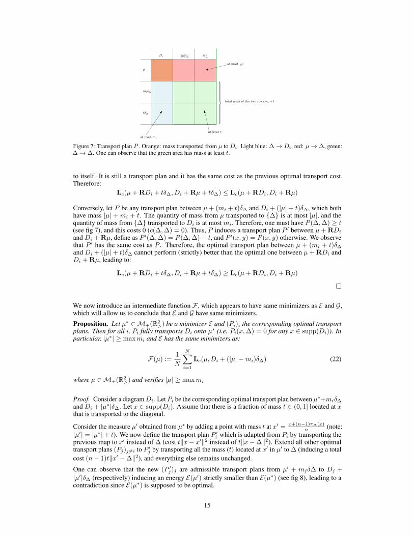
Figure 7: Transport plan P . Orange: mass transported from µ to Di. Light blue: ∆→ Di, red: µ→ ∆, green:∆→ ∆. One can observe that the green area has mass at least t.
to itself. It is still a transport plan and it has the same cost as the previous optimal transport cost.Therefore:
Lc(µ+ RDi + tδ∆, Di + Rµ+ tδ∆) ≤ Lc(µ+ RDi, Di + Rµ)
Conversely, let P be any transport plan between µ+ (mi + t)δ∆ and Di + (|µ|+ t)δ∆, which bothhave mass |µ| + mi + t. The quantity of mass from µ transported to {∆} is at most |µ|, and thequantity of mass from {∆} transported to Di is at most mi. Therefore, one must have P (∆,∆) ≥ t(see fig 7), and this costs 0 (c(∆,∆) = 0). Thus, P induces a transport plan P ′ between µ+ RDi
and Di + Rµ, define as P ′(∆,∆) = P (∆,∆)− t, and P ′(x, y) = P (x, y) otherwise. We observethat P ′ has the same cost as P . Therefore, the optimal transport plan between µ + (mi + t)δ∆and Di + (|µ|+ t)δ∆ cannot perform (strictly) better than the optimal one between µ+ RDi andDi + Rµ, leading to:
Lc(µ+ RDi + tδ∆, Di + Rµ+ tδ∆) ≥ Lc(µ+ RDi, Di + Rµ)
We now introduce an intermediate function F , which appears to have same minimizers as E and G,which will allow us to conclude that E and G have same minimizers.
Proposition. Let µ∗ ∈M+(R2>) be a minimizer E and (Pi)i the corresponding optimal transport
plans. Then for all i, Pi fully transports Di onto µ∗ (i.e. Pi(x,∆) = 0 for any x ∈ supp(Di)). Inparticular, |µ∗| ≥ maxmi and E has the same minimizers as:
F(µ) :=1
N
N∑
i=1
Lc(µ,Di + (|µ| −mi)δ∆) (22)
where µ ∈M+(R2>) and verifies |µ| ≥ maxmi
Proof. Consider a diagramDi. LetPi be the corresponding optimal transport plan between µ∗+miδ∆and Di + |µ∗|δ∆. Let x ∈ supp(Di). Assume that there is a fraction of mass t ∈ (0, 1] located at xthat is transported to the diagonal.
Consider the measure µ′ obtained from µ∗ by adding a point with mass t at x′ = x+(n−1)π∆(x)n (note:
|µ′| = |µ∗|+ t). We now define the transport plan P ′i which is adapted from Pi by transporting theprevious map to x′ instead of ∆ (cost t‖x− x′‖2 instead of t‖x−∆‖2). Extend all other optimaltransport plans (Pj)j 6=i to P ′j by transporting all the mass (t) located at x′ in µ′ to ∆ (inducing a totalcost (n− 1)t‖x′ −∆‖2), and everything else remains unchanged.
One can observe that the new (P ′j)j are admissible transport plans from µ′ + mjδ∆ to Dj +|µ′|δ∆ (respectively) inducing an energy E(µ′) strictly smaller than E(µ∗) (see fig 8), leading to acontradiction since E(µ∗) is supposed to be optimal.
15

tδx
π∆(x)
t
tδx′
BeforeAfter
t
t
Figure 8: Illustration of the proof. The cost induced by the green matching is strictly better than the red one.
To prove equivalence between the two problems considered (in the sense that they have the sameminimizers), we introduce µ∗E and µ∗F which are minimizers of E and F respectively. We first observethat F(µ) ≤ E(µ) for all µ (adding the same amount of mass on ∆ can only decrease the optimaltransport cost).
This allows us to write:
F(µ∗E) = E(µ∗E) We can remove miδ∆ from both sides≤ E(µ∗F ) since µ∗E is a minimizer of E≤ F(µ∗F ) since E(µ) ≤ F(µ)
≤ F(µ∗E) since µ∗F is a minimizer of FHence, all these inequalities are actually equalities, thus minimizers of E are minimizers of F andvice-versa.
We can now prove that F as the same minimizers as G which will finally prove Theorem 1.
Proof. Let µ∗G be a minimizer of G. Consider µ∆ := (mtot − |µ∗G |)δ∆. We observe that µ∆ isalways transported on {∆} (inducing a cost of 0) for each of the transport plan Pi ∈ Π(µ∗G +µ∆, Di)for minimality considerations (as in previous proof). Observe also (as in previous proof) thatG(µ) ≤ F(µ) for any measure µ.
G(µ∗G) = F(µ∗G) remove µ∆ from both sides≥ F(µ∗F ) since µ∗F is a minimizer of F≥ G(µ∗F ) since G(µ) ≤ F(µ)
≥ G(µ∗G) since µ∗G is a minimizer of GThis implies that minimizers of G are minimizers of F (and thus of E) and conversely.
We now give details about the Corollary of Theorem 1.
Proof of Corollary.
(i) Given N diagrams D1 . . . DN and (x1 . . . xN ) ∈ supp(D1) × · · · × supp(DN ), amongwhich k of them are equals to ∆, on can easily observe (this is mentioned in Turner et al.(2014)) that z 7→∑N
i=1 ‖z − xi‖22 admits a unique minimizer x∗ = (N−k)x+kπ∆(x)N , where
x is the arithmetic mean of the (N − k) non-diagonal points in x1 . . . xN .
The localization property (see §2.2 of Carlier et al. (2015)) states that the support of anybarycenter is included in the set S of such x∗s which is finite, proving in particular thatbarycenters of D1 . . . DN have a discrete support included in some known set. Note that asimilar result is also mentioned in (Anderes et al., 2016).
16

(ii) As a consequence of previous point, one can describe a barycenter of D1 . . . DN as a vectorof weight w ∈ Rs+, where s is the cardinality of S and cast the barycenter problem as aLinear Programming (LP) one (see for example §3.2 in (Anderes et al., 2016) or §2.3 and2.4 in (Carlier et al., 2015)). More precisely, the problem is equivalent to:
minimizew∈Rs+
wT c
s.t.∀i = 1 . . . N,Aiw = bi
Here, c ∈ Rs is defined as cj =∑Nk=1 ‖x∗j − xk,j‖22, where x∗j is the mean (as defined
above) associated to (xk,j)Nk=1. The constraints correspond to marginals constraints: bi
is the weight vector associated to Di on each point of its support. Note that each bi hasinteger coordinates and that Ai is totally unimodular (see (Schrijver, 1998)), and thus amongoptimal w, some of them have integer coordinate.
Bad local minima of E . The following lemma illustrate specific situation which lead algorithmsproposed by Turner et al. to get stuck in bad local minima.
Lemma 1. For any κ ≥ 1, there exists a set of diagrams such that E admits a local minimizer Dloc
verifying:E(Dloc) ≥ κE(Dopt)
where Dopt is a global minimizer. Furthermore, there exist sets of diagrams so that the B-Munkresalgorithm always converges to such a local minimum when initialized with one of the input diagram.
births
deaths
2√ε
1
(a) Example of arbitrary bad local minima of E .Blue point and green point represent our two dia-grams of interest. Red point is a global minimizerof E . The two orange points give a diagram whichis a local minimizer of E achieving an energy ar-bitrary higher (relatively) than the one of the reddiagram (as ε goes to 0).
births
deaths
(b) Failing configuration for B-Munkres algorithm.Three diagrams (red, blue, green) along with theoutput of Turner et al algorithm (purple) wheninitialized on the green diagram (we have similarresult by symmetry when initialized on any otherdiagram).
Figure 9: Example of simple configurations in which the B-Munkres algorithm will converge to arbitrarily badlocal minima
Proof. We consider the configuration of Fig. 9a where we consider two diagrams with 1 point (blueand green diagram) and their correct barycenter (red diagram) along with the orange diagram (2points). It is easy to observe that when restricted to the space of persistence diagram, the orangediagram is a minimizer of the function E (in which the algorithm could get stuck if initialized poorly).It achieves an energy of 1
2 (( 12 + 1
2 )2 + ( 12 + 1
2 )2) = 1 while the red diagram achieves an energy of12 (√ε2
+√ε2) = ε. This example proves that there exist configurations of diagrams so that E has
arbitrary bad local minima.
17

One could argue that when initialized to one of the input diagram (as suggested in (Turner et al.,2014)), the algorithm will not get stuck to the orange diagram. Fig. 9b provide a configurationinvolving three diagrams with two points each where the algorithm will always get stuck in a badlocal minimum when initialized with any of the three diagrams. The analysis is similar to previousstatement.
18