Embed Size (px)
Citation preview
Laplacian Matrices of Graphs:Algorithms and Applications
ICML, June 21, 2016
Daniel A. Spielman
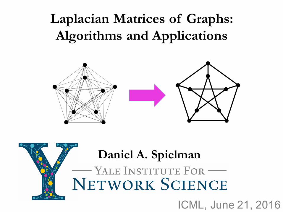
LaplaciansInterpolation on graphsSpring networksClusteringIsotonic regression
Sparsification
Solving Laplacian EquationsBest resultsThe simplest algorithm
Outline
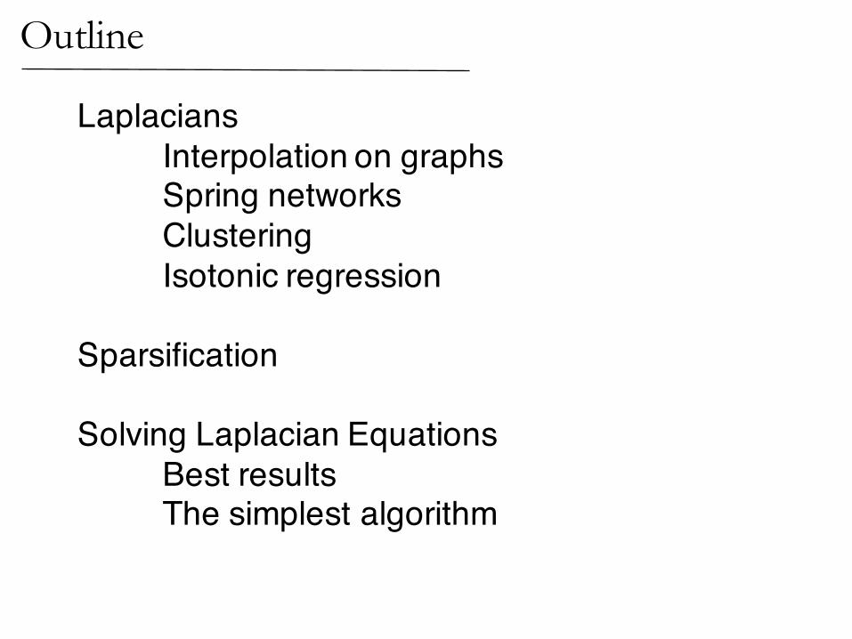
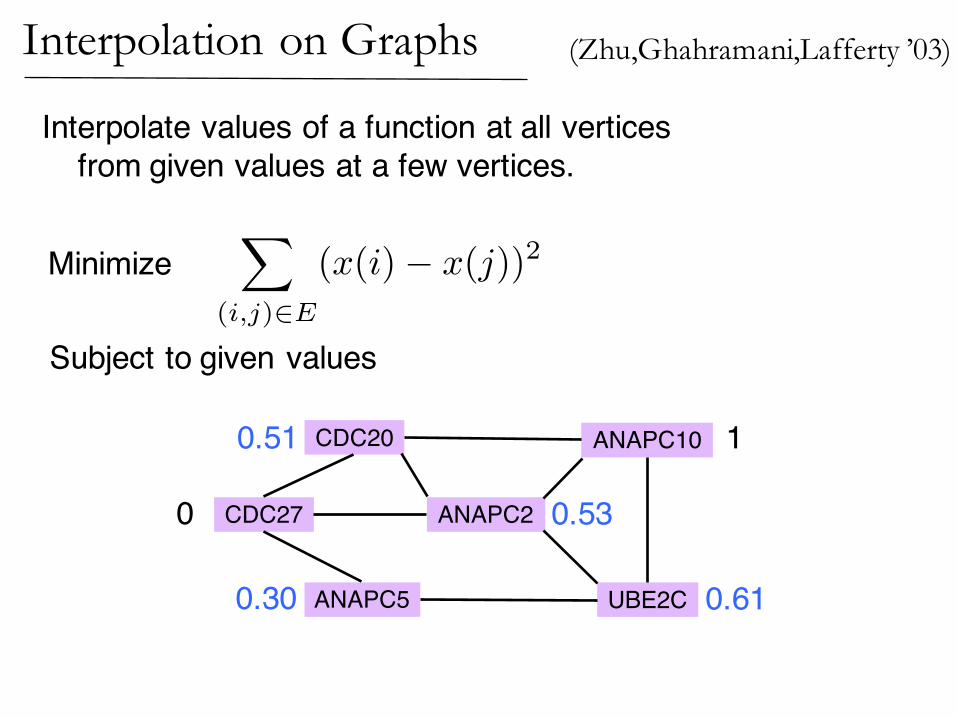
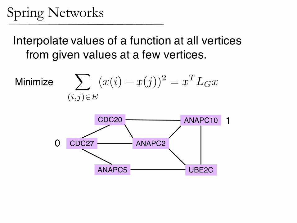
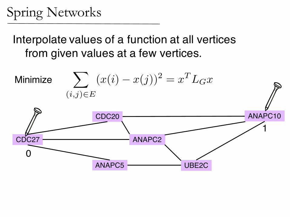
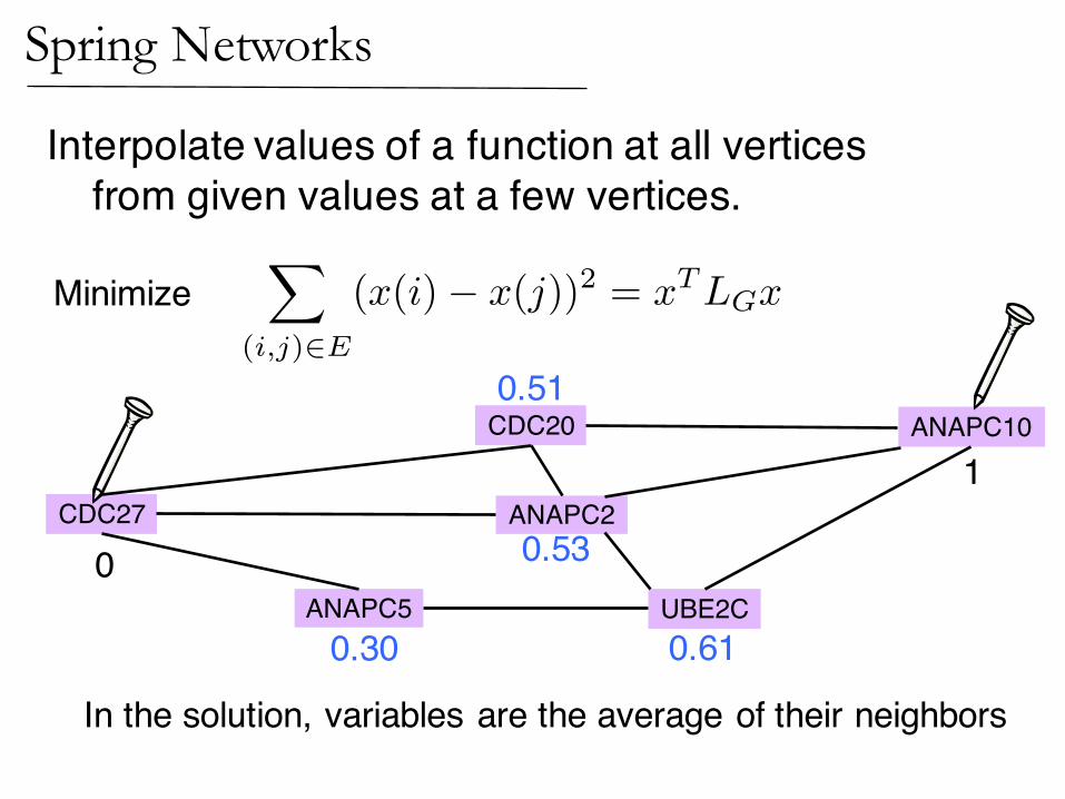
Interpolate values of a function at all verticesfrom given values at a few vertices.
Minimize
Subject to given values
1
0
ANAPC10
CDC27
ANAPC5 UBE2C
ANAPC2
CDC20
(Zhu,Ghahramani,Lafferty ’03)Interpolation on Graphs
X
(i,j)2E
(x(i)� x(j))2
Interpolate values of a function at all verticesfrom given values at a few vertices.
Minimize
Subject to given values
1
0
0.51
0.61
0.53
0.30
ANAPC10
CDC27
ANAPC5 UBE2C
ANAPC2
CDC20
(Zhu,Ghahramani,Lafferty ’03)Interpolation on Graphs
X
(i,j)2E
(x(i)� x(j))2
X
(i,j)2E
(x(i)� x(j))2 = x
TLGx
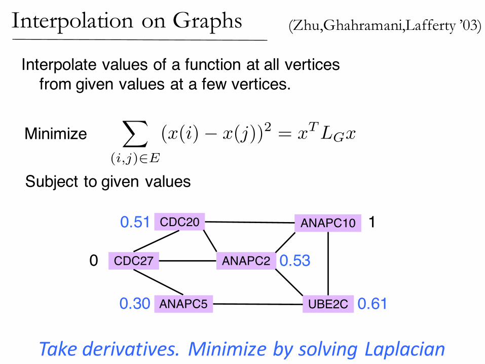
Interpolate values of a function at all verticesfrom given values at a few vertices.
Minimize
Subject to given values
Takederivatives.MinimizebysolvingLaplacian
1
0
0.51
0.61
0.53
0.30
ANAPC10
CDC27
ANAPC5 UBE2C
ANAPC2
CDC20
(Zhu,Ghahramani,Lafferty ’03)Interpolation on Graphs
X
(i,j)2E
(x(i)� x(j))2 = x
TLGx
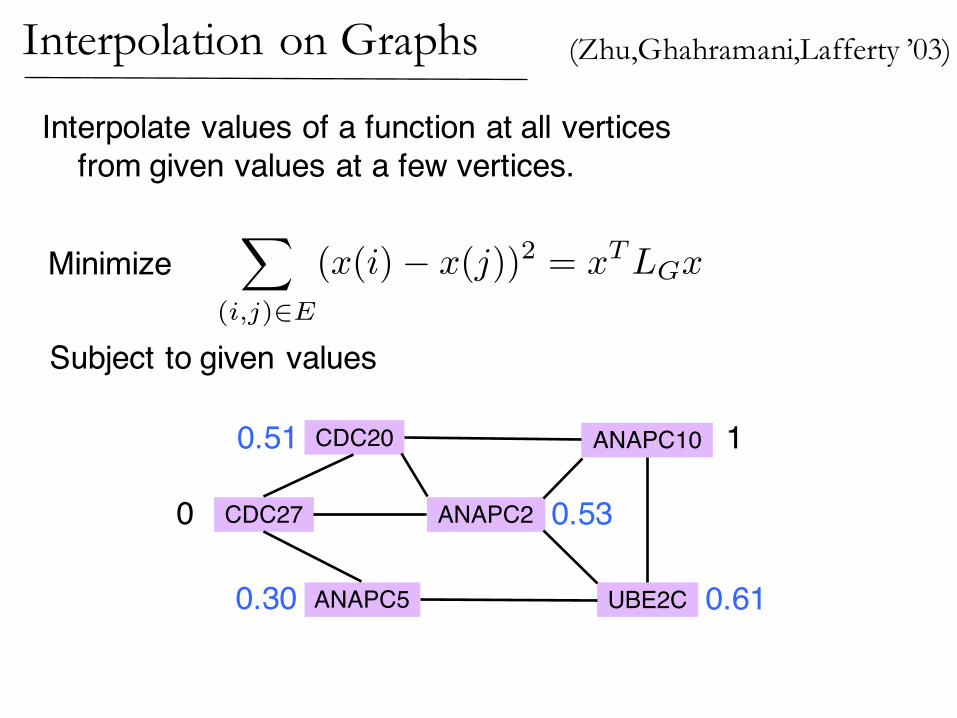
Interpolate values of a function at all verticesfrom given values at a few vertices.
Minimize
Subject to given values
1
0
0.51
0.61
0.53
0.30
ANAPC10
CDC27
ANAPC5 UBE2C
ANAPC2
CDC20
(Zhu,Ghahramani,Lafferty ’03)Interpolation on Graphs
X
(i,j)2E
(x(i)� x(j))2
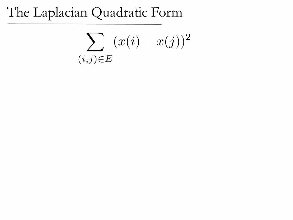
The Laplacian Quadratic Form

x
TLGx =
X
(i,j)2E
(x(i)� x(j))2
The Laplacian Matrix of a Graph
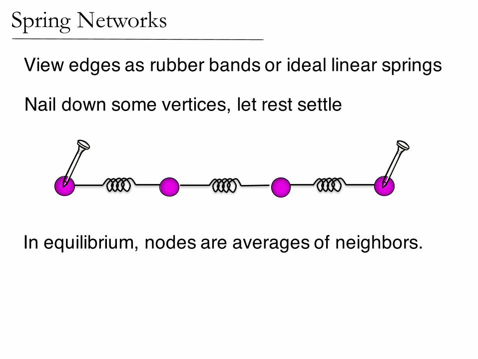
Nail down some vertices, let rest settle
View edges as rubber bands or ideal linear springs
In equilibrium, nodes are averages of neighbors.
Spring Networks
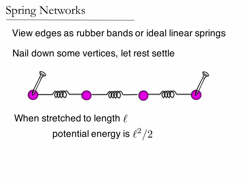
Nail down some vertices, let rest settle
View edges as rubber bands or ideal linear springs
Spring Networks
When stretched to length potential energy is
`
�2/2
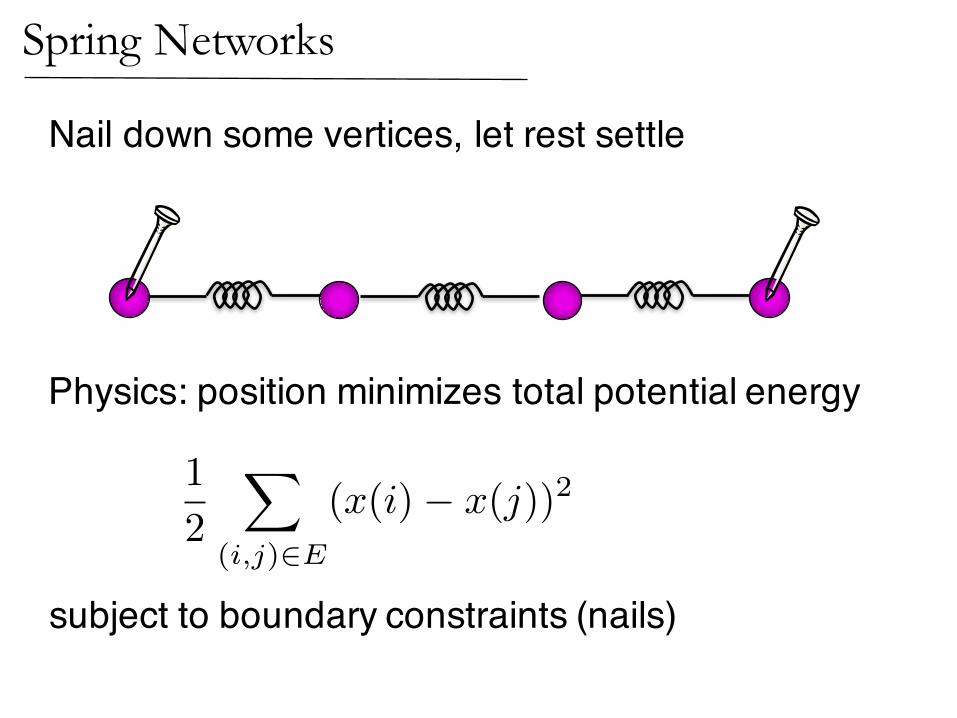
Nail down some vertices, let rest settle
Physics: position minimizes total potential energy
subject to boundary constraints (nails)
Spring Networks
1
2
X
(i,j)2E
(x(i)� x(j))2
X
(i,j)2E
(x(i)� x(j))2 = x
TLGx
0
ANAPC10
CDC27
ANAPC5 UBE2C
ANAPC2
CDC20
Spring Networks
Interpolate values of a function at all verticesfrom given values at a few vertices.
Minimize
1
1
0
ANAPC10
CDC27
ANAPC5 UBE2C
ANAPC2
CDC20
Spring Networks
Interpolate values of a function at all verticesfrom given values at a few vertices.
MinimizeX
(i,j)2E
(x(i)� x(j))2 = x
TLGx
X
(i,j)2E
(x(i)� x(j))2 = x
TLGx
Interpolate values of a function at all verticesfrom given values at a few vertices.
Minimize
1
0
0.51
0.61
0.53
0.30
ANAPC10
CDC27
ANAPC5 UBE2C
ANAPC2
CDC20
Spring Networks
In the solution, variables are the average of their neighbors
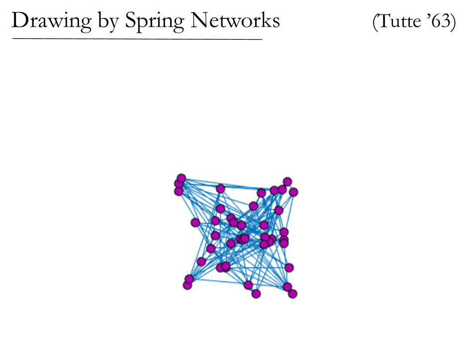
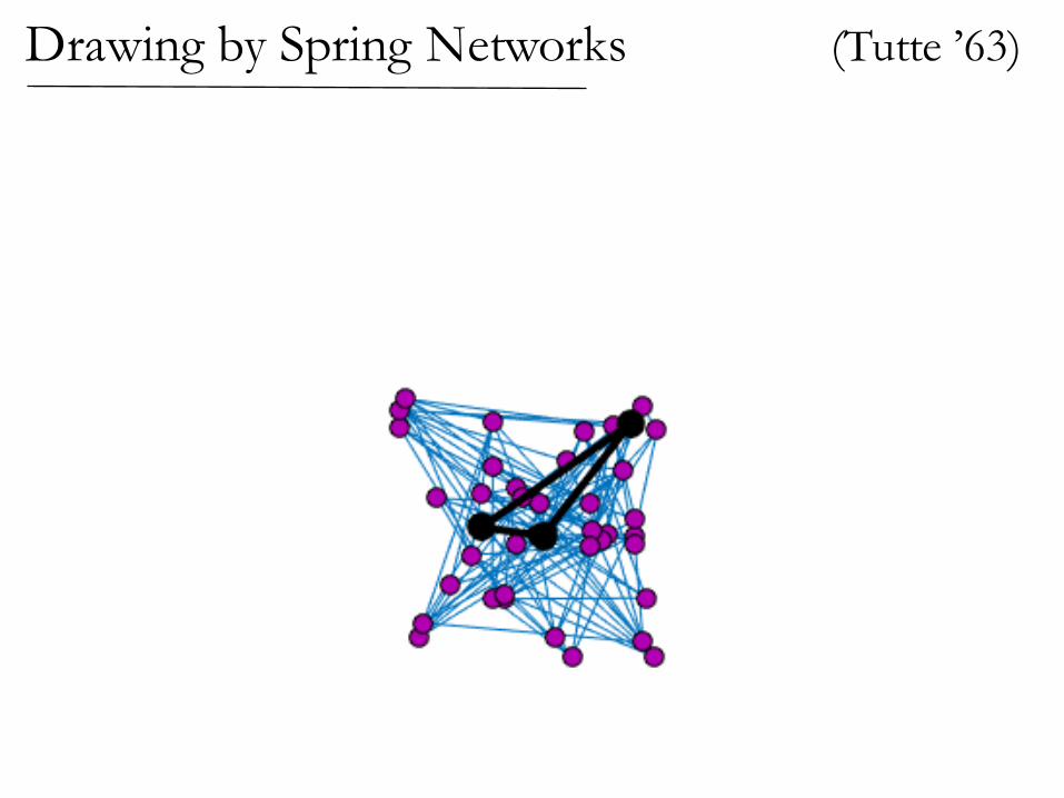
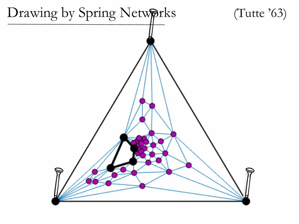
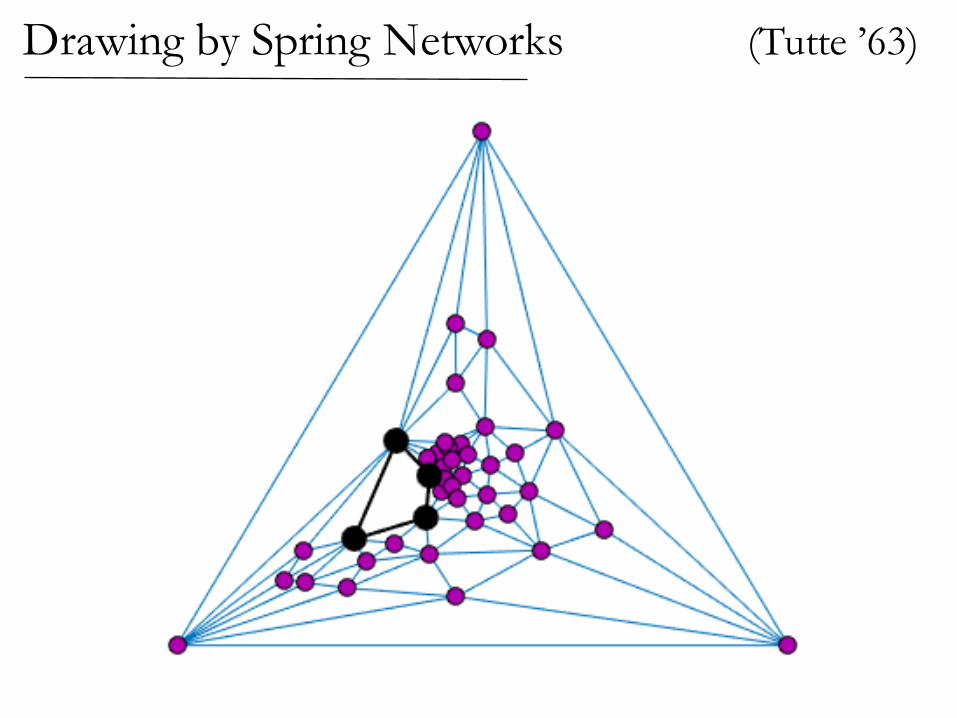
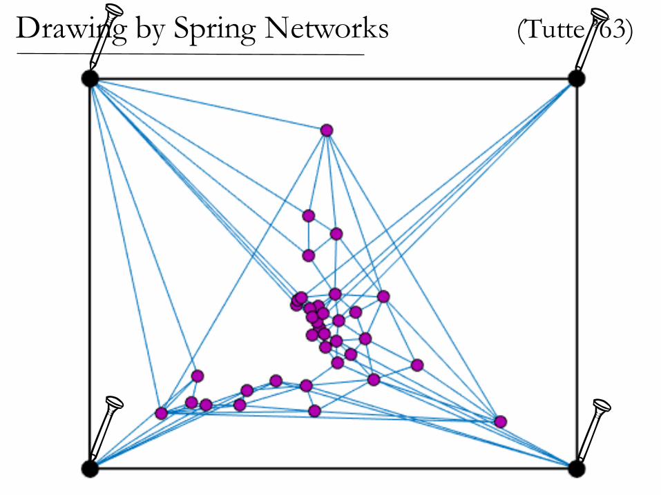
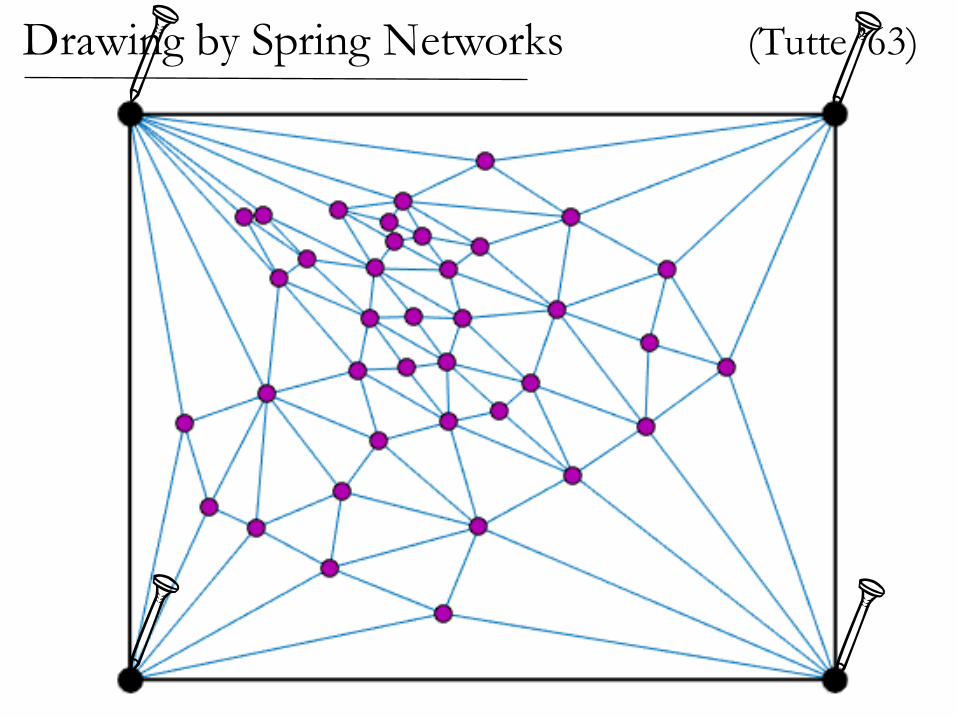
(Tutte ’63)Drawing by Spring Networks
Drawing by Spring Networks (Tutte ’63)
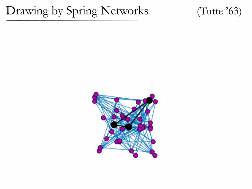
Drawing by Spring Networks (Tutte ’63)
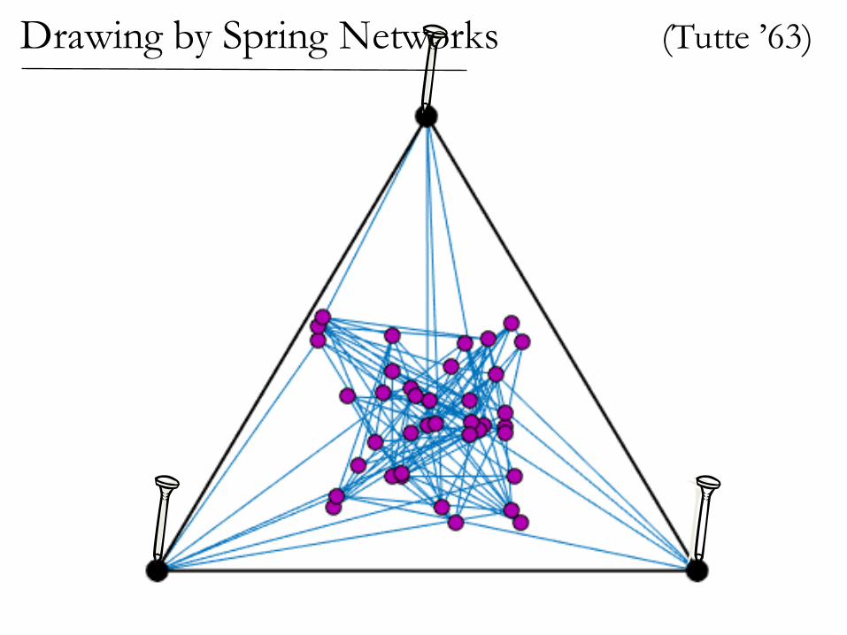
Drawing by Spring Networks (Tutte ’63)
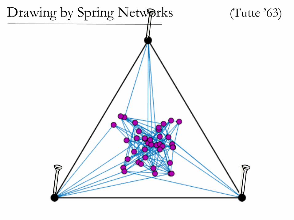
Drawing by Spring Networks (Tutte ’63)

If the graph is planar,then the spring drawinghas no crossing edges!
Drawing by Spring Networks (Tutte ’63)
Drawing by Spring Networks (Tutte ’63)
Drawing by Spring Networks (Tutte ’63)

Drawing by Spring Networks (Tutte ’63)
Drawing by Spring Networks (Tutte ’63)
Drawing by Spring Networks (Tutte ’63)
SS
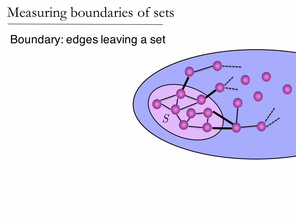
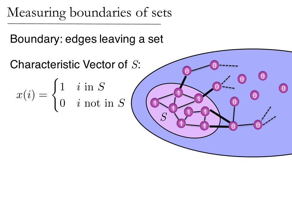
Measuring boundaries of sets
Boundary: edges leaving a set
Boundary: edges leaving a set
S
00
00
00
1
1 0
11
11 1
0
00
1
S
Characteristic Vector of S:
x(i) =
(1 i in S
0 i not in S
Measuring boundaries of sets
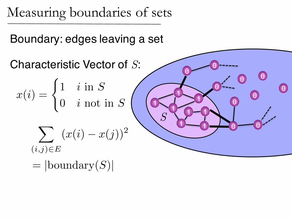
Boundary: edges leaving a set
S
00
00
00
1
1 0
11
11 1
0
00
1
S
Characteristic Vector of S:
x(i) =
(1 i in S
0 i not in S
Measuring boundaries of sets
X
(i,j)2E
(x(i)� x(j))
2
= |boundary(S)|
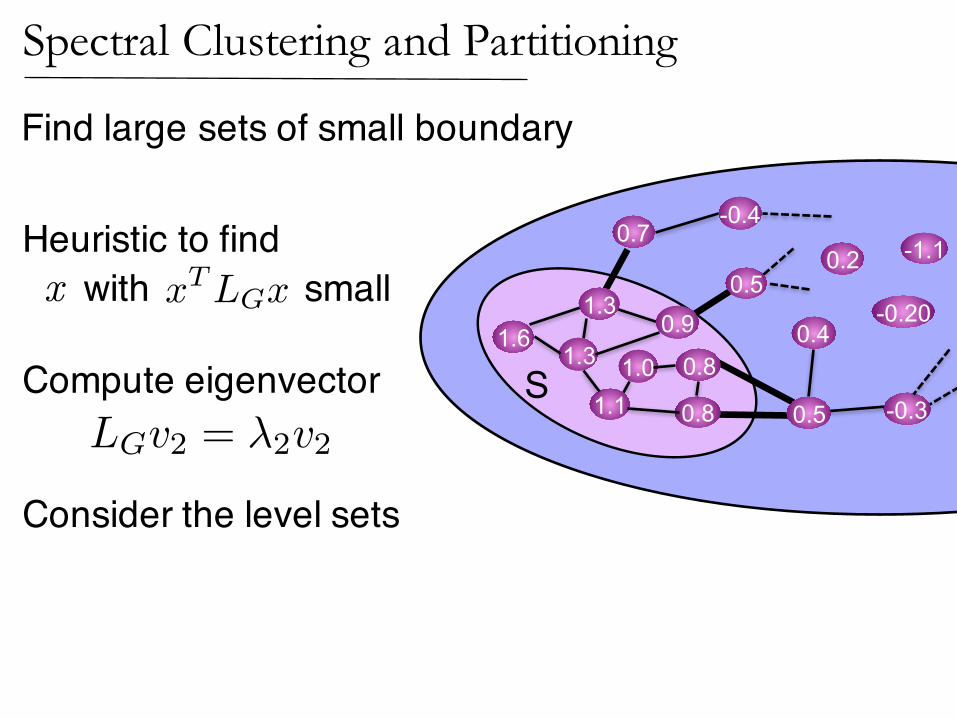
Find large sets of small boundary
S
0.2
-0.200.4
-1.10.5
0.8
0.81.11.0
1.61.3
0.9
0.7-0.4
-0.3
1.3
S0.5
Heuristic to findx with small
Compute eigenvector
Consider the level sets
LGv2 = �2v2
x
TLGx
Spectral Clustering and Partitioning
2
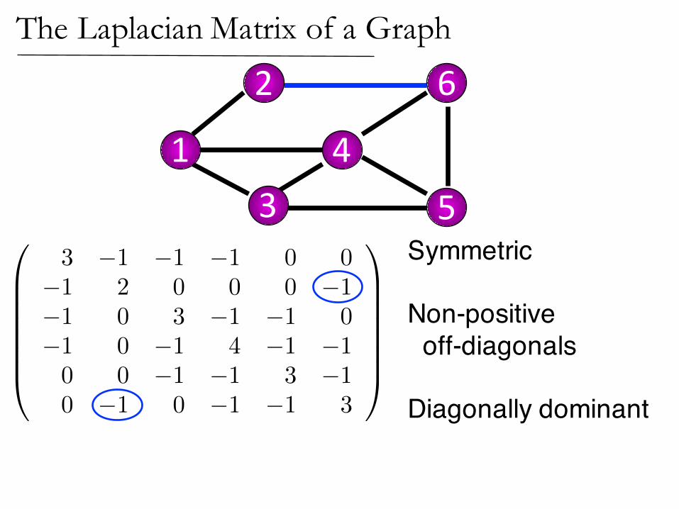
1 43 5
6
0
BBBBBB@
3 �1 �1 �1 0 0�1 2 0 0 0 �1�1 0 3 �1 �1 0�1 0 �1 4 �1 �10 0 �1 �1 3 �10 �1 0 �1 �1 3
1
CCCCCCA
Symmetric
Non-positive off-diagonals
Diagonally dominant
The Laplacian Matrix of a Graph
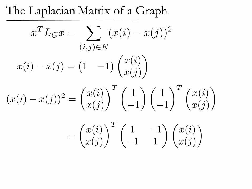
x
TLGx =
X
(i,j)2E
(x(i)� x(j))2
x(i)� x(j) =�1 �1
�✓x(i)x(j)
◆
=
✓x(i)x(j)
◆T ✓1 �1�1 1
◆✓x(i)x(j)
◆
The Laplacian Matrix of a Graph
(x(i)� x(j))2 =
✓x(i)x(j)
◆T ✓1�1
◆✓1�1
◆T ✓x(i)x(j)
◆
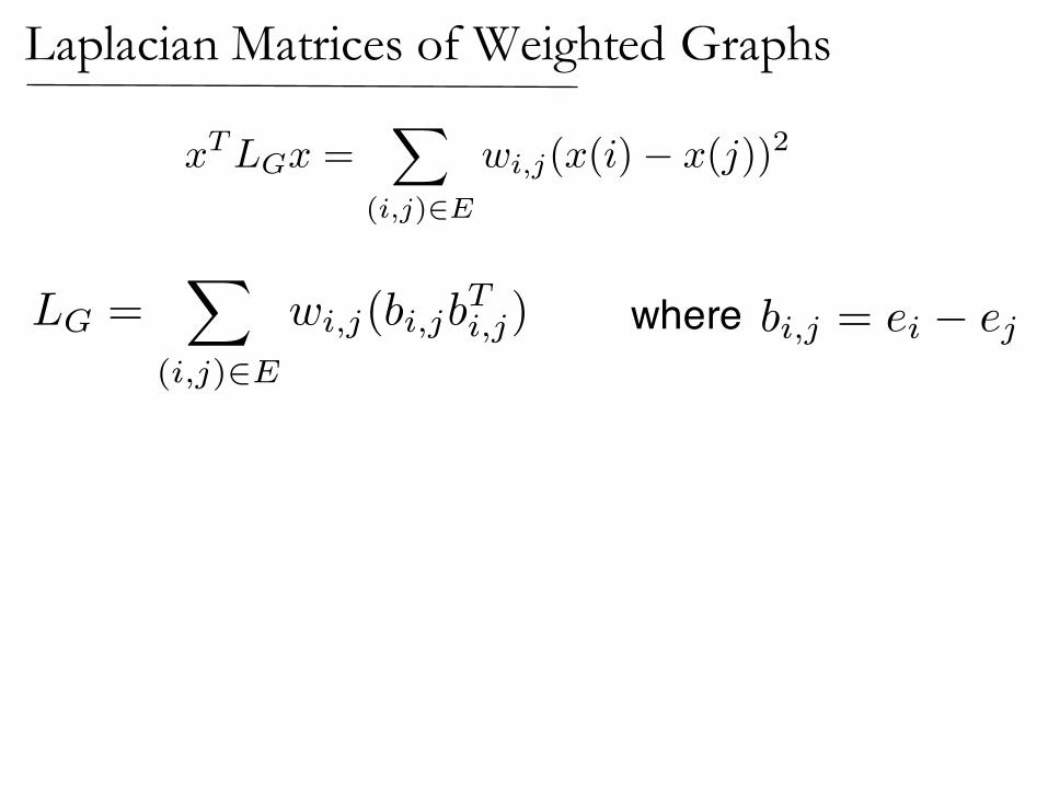
x
TLGx =
X
(i,j)2E
wi,j(x(i)� x(j))2
Laplacian Matrices of Weighted Graphs
LG =X
(i,j)2E
wi,j(bi,jbTi,j) where bi,j = ei � ej
B is the signed edge-vertex adjacency matrixwith one row for each
W is the diagonal matrix of weights
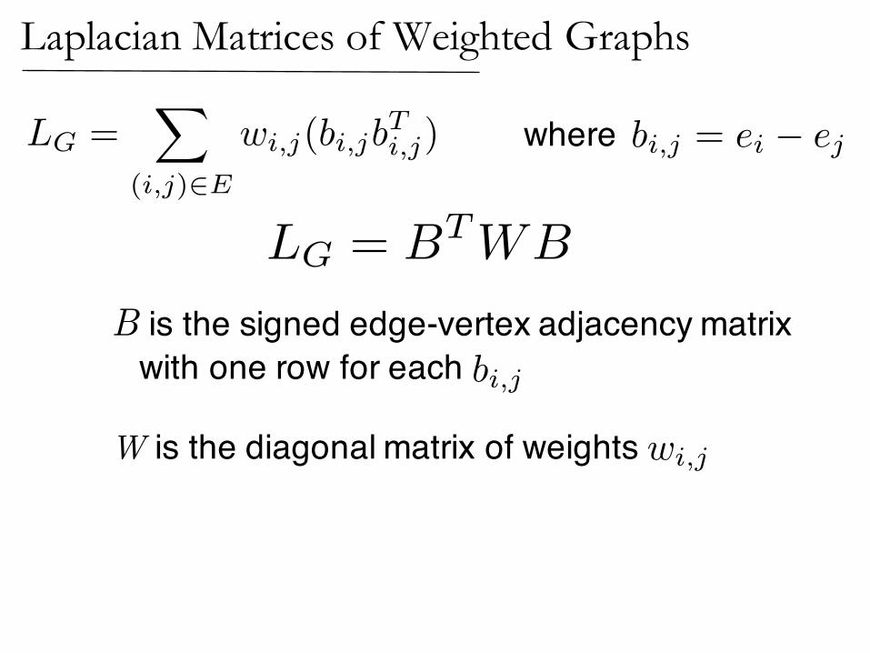
LG =X
(i,j)2E
wi,j(bi,jbTi,j)
bi,j
wi,j
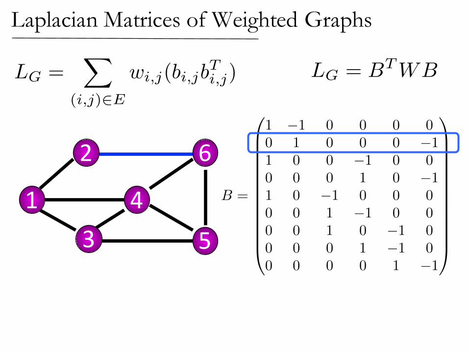
LG = BTWB
Laplacian Matrices of Weighted Graphs
where bi,j = ei � ej
LG = BTWB
Laplacian Matrices of Weighted Graphs
B =
0
BBBBBBBBBBBB@
1 �1 0 0 0 00 1 0 0 0 �11 0 0 �1 0 00 0 0 1 0 �11 0 �1 0 0 00 0 1 �1 0 00 0 1 0 �1 00 0 0 1 �1 00 0 0 0 1 �1
1
CCCCCCCCCCCCA
2
1 43 5
6
LG =X
(i,j)2E
wi,j(bi,jbTi,j)
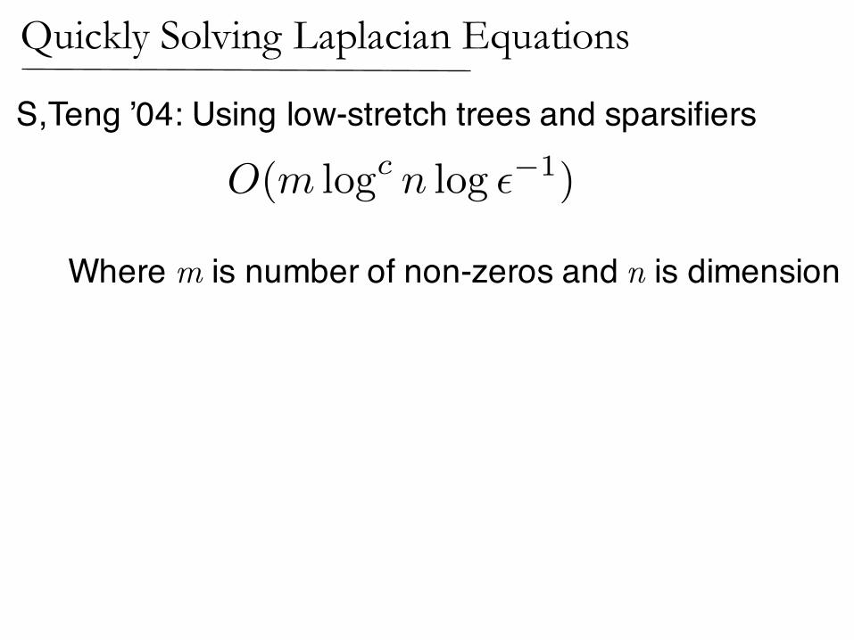
Quickly Solving Laplacian Equations
Where m is number of non-zeros and n is dimension
O(m log
c n log ✏�1)
S,Teng ’04: Using low-stretch trees and sparsifiers
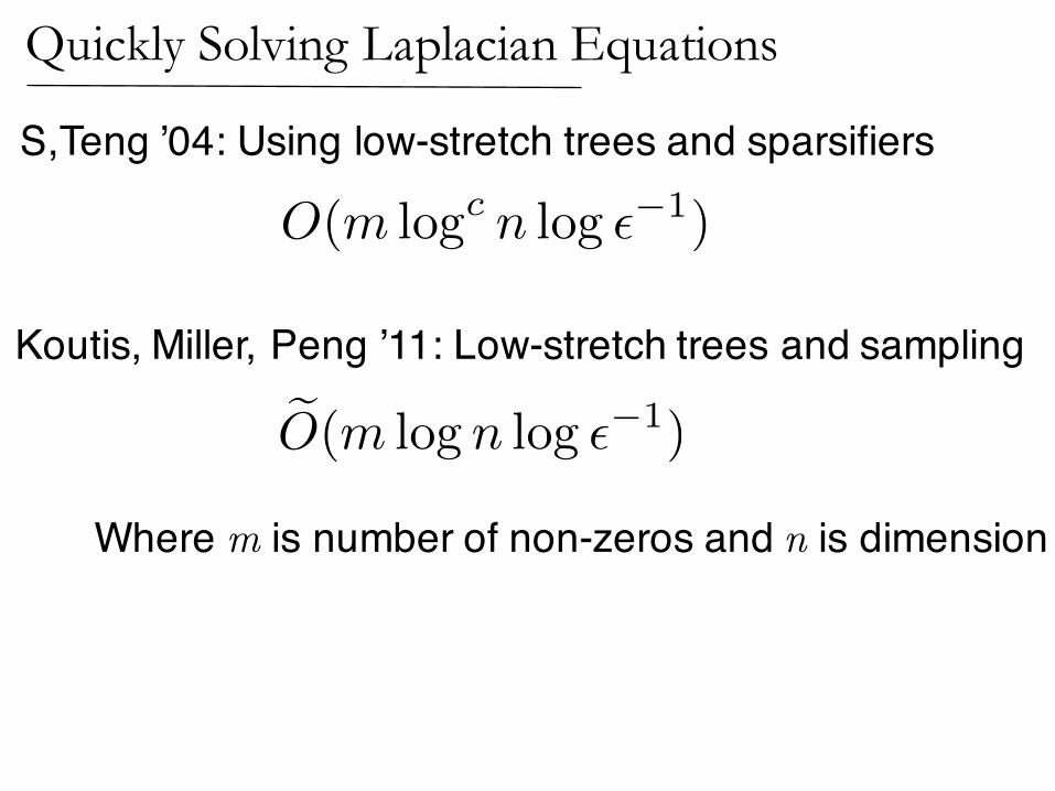
Where m is number of non-zeros and n is dimension
O(m log
c n log ✏�1)
eO(m log n log ✏�1)
Koutis, Miller, Peng ’11: Low-stretch trees and sampling
S,Teng ’04: Using low-stretch trees and sparsifiers
Quickly Solving Laplacian Equations
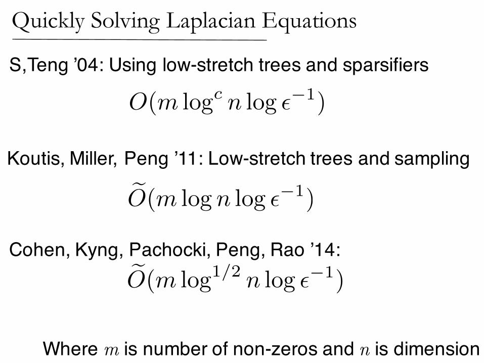
Where m is number of non-zeros and n is dimension
Cohen, Kyng, Pachocki, Peng, Rao ’14:
O(m log
c n log ✏�1)
eO(m log n log ✏�1)
eO(m log
1/2 n log ✏�1)
Koutis, Miller, Peng ’11: Low-stretch trees and sampling
S,Teng ’04: Using low-stretch trees and sparsifiers
Quickly Solving Laplacian Equations
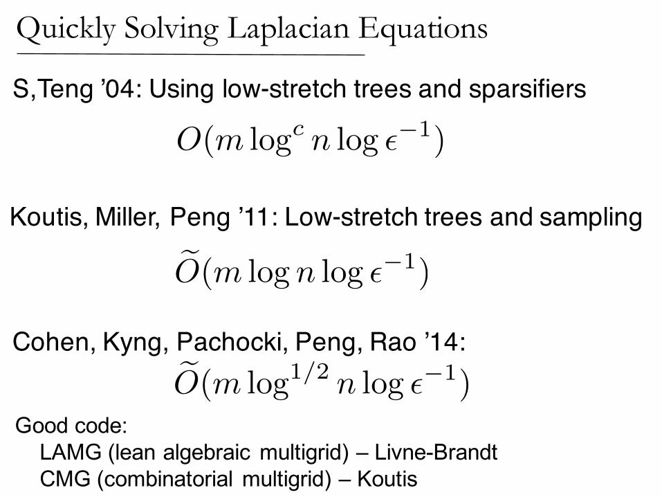
Cohen, Kyng, Pachocki, Peng, Rao ’14:
O(m log
c n log ✏�1)
eO(m log n log ✏�1)
eO(m log
1/2 n log ✏�1)
Koutis, Miller, Peng ’11: Low-stretch trees and sampling
S,Teng ’04: Using low-stretch trees and sparsifiers
Quickly Solving Laplacian Equations
Good code:LAMG (lean algebraic multigrid) – Livne-BrandtCMG (combinatorial multigrid) – Koutis
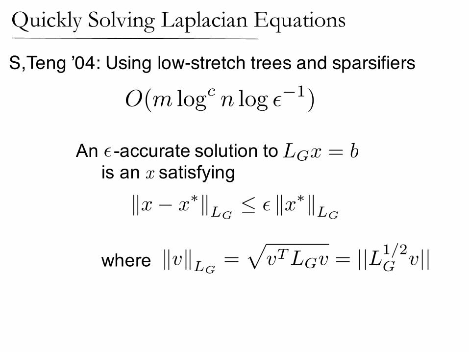
An -accurate solution to is an x satisfying
where
LGx = b
✏
kvkLG=
pvTLGv = ||L1/2
G v||
Quickly Solving Laplacian Equations
O(m log
c n log ✏�1)
S,Teng ’04: Using low-stretch trees and sparsifiers
kx� x
⇤kLG ✏ kx⇤kLG
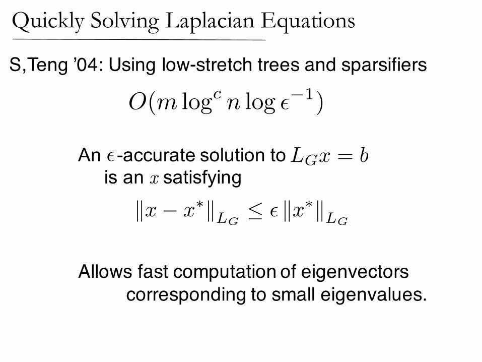
An -accurate solution to is an x satisfying
LGx = b
✏
Quickly Solving Laplacian Equations
O(m log
c n log ✏�1)
S,Teng ’04: Using low-stretch trees and sparsifiers
kx� x
⇤kLG ✏ kx⇤kLG
Allows fast computation of eigenvectorscorresponding to small eigenvalues.
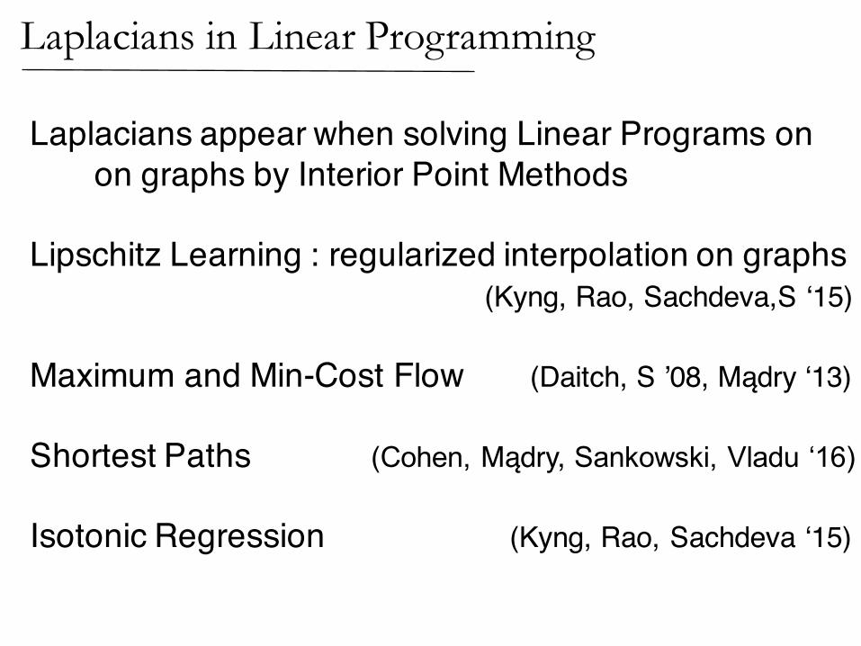
Laplacians appear when solving Linear Programs onon graphs by Interior Point Methods
Lipschitz Learning : regularized interpolation on graphs(Kyng, Rao, Sachdeva,S ‘15)
Maximum and Min-Cost Flow (Daitch, S ’08, Mądry ‘13)
Shortest Paths (Cohen, Mądry, Sankowski, Vladu ‘16)
Isotonic Regression (Kyng, Rao, Sachdeva ‘15)
Laplacians in Linear Programming
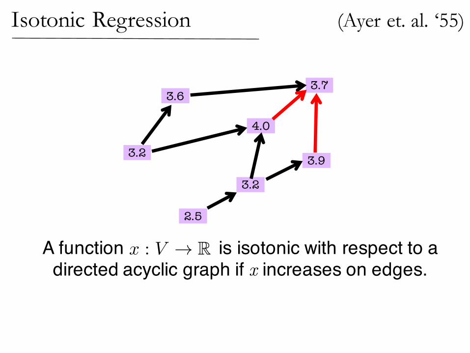
(Ayer et. al. ‘55)Isotonic Regression
2.5
3.2
3.2
4.0
3.73.6
3.9
A function is isotonic with respect to a directed acyclic graph if x increases on edges.
x : V ! R
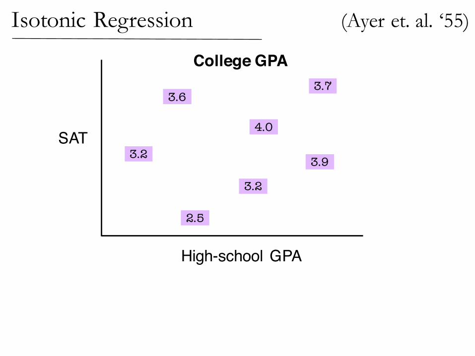
Isotonic Regression
2.5
3.2
3.2
4.0
3.73.6
3.9
College GPA
High-school GPA
SAT
(Ayer et. al. ‘55)
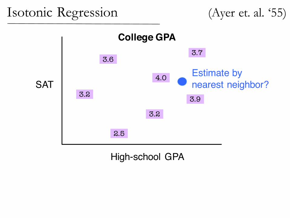
Isotonic Regression
2.5
3.2
3.2
4.0
3.73.6
3.9
College GPA
High-school GPA
SATEstimate bynearest neighbor?
(Ayer et. al. ‘55)
Isotonic Regression
2.5
3.2
3.2
4.0
3.73.6
3.9
College GPA
High-school GPA
SATEstimate bynearest neighbor?
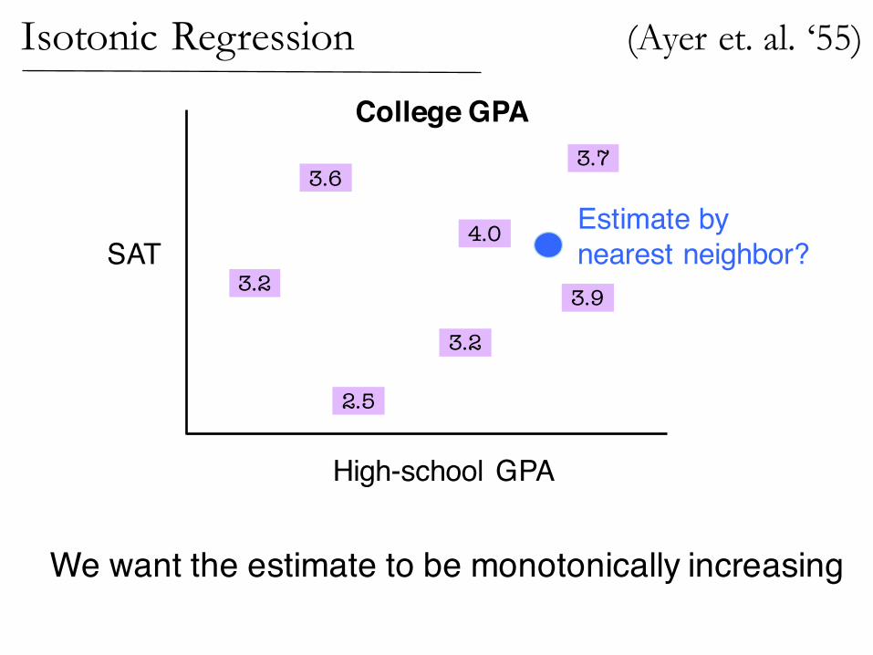
We want the estimate to be monotonically increasing
(Ayer et. al. ‘55)
Isotonic Regression
2.5
3.2
3.2
4.0
3.73.6
3.9
College GPA
High-school GPA
SAT
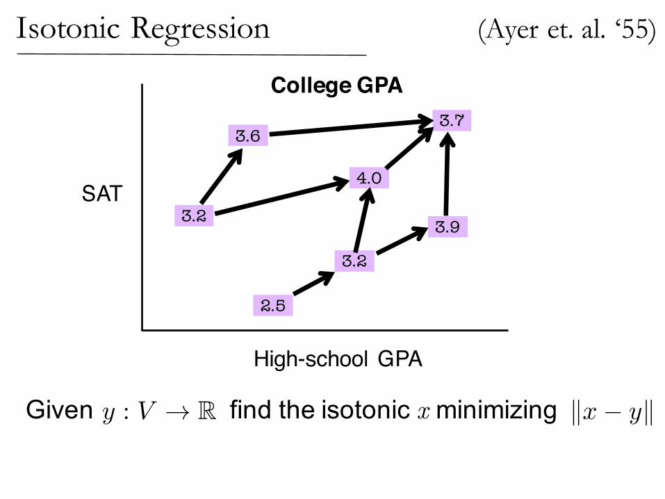
Given find the isotonic x minimizingy : V ! R kx� yk
(Ayer et. al. ‘55)
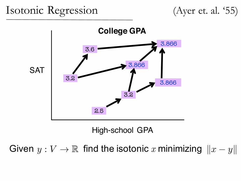
Isotonic Regression
2.5
3.2
3.2
3.866
3.8663.6
3.866
College GPA
High-school GPA
SAT
(Ayer et. al. ‘55)
Given find the isotonic x minimizingy : V ! R kx� yk
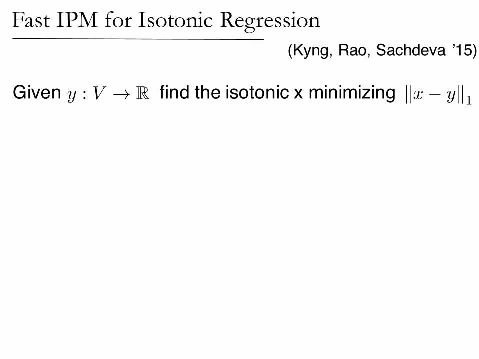
Given find the isotonic x minimizingy : V ! R kx� yk1
(Kyng, Rao, Sachdeva ’15)Fast IPM for Isotonic Regression
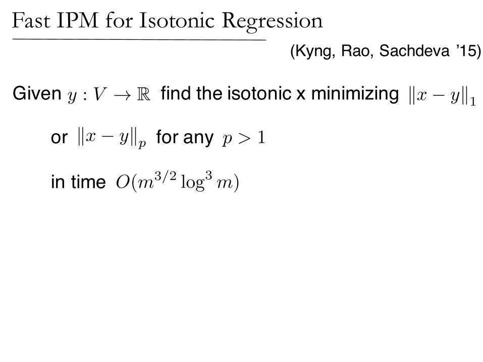
Given find the isotonic x minimizingy : V ! R kx� yk1
or for any
in time
kx� ykp p > 1
O(m3/2log
3 m)
(Kyng, Rao, Sachdeva ’15)Fast IPM for Isotonic Regression
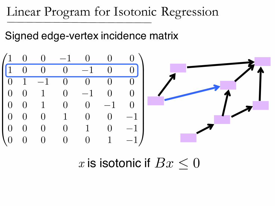
Signed edge-vertex incidence matrix
x is isotonic if Bx 0
B =
0
BBBBBBBBBB@
1 0 0 �1 0 0 01 0 0 0 �1 0 00 1 �1 0 0 0 00 0 1 0 �1 0 00 0 1 0 0 �1 00 0 0 1 0 0 �10 0 0 0 1 0 �10 0 0 0 0 1 �1
1
CCCCCCCCCCA
Linear Program for Isotonic Regression
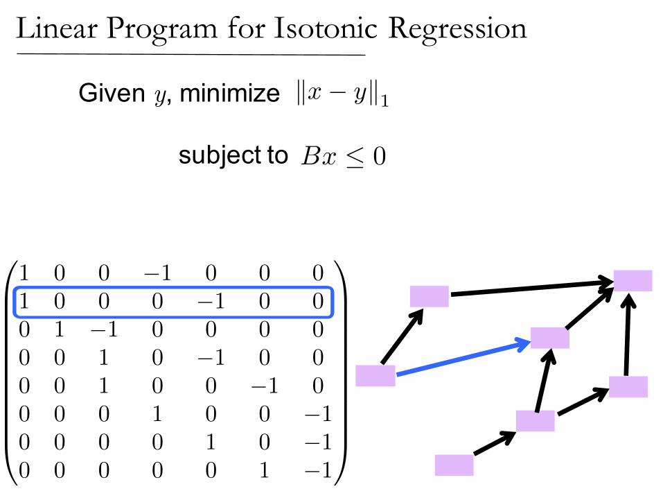
Given y, minimize
subject to
kx� yk1
Bx 0
B =
0
BBBBBBBBBB@
1 0 0 �1 0 0 01 0 0 0 �1 0 00 1 �1 0 0 0 00 0 1 0 �1 0 00 0 1 0 0 �1 00 0 0 1 0 0 �10 0 0 0 1 0 �10 0 0 0 0 1 �1
1
CCCCCCCCCCA
Linear Program for Isotonic Regression
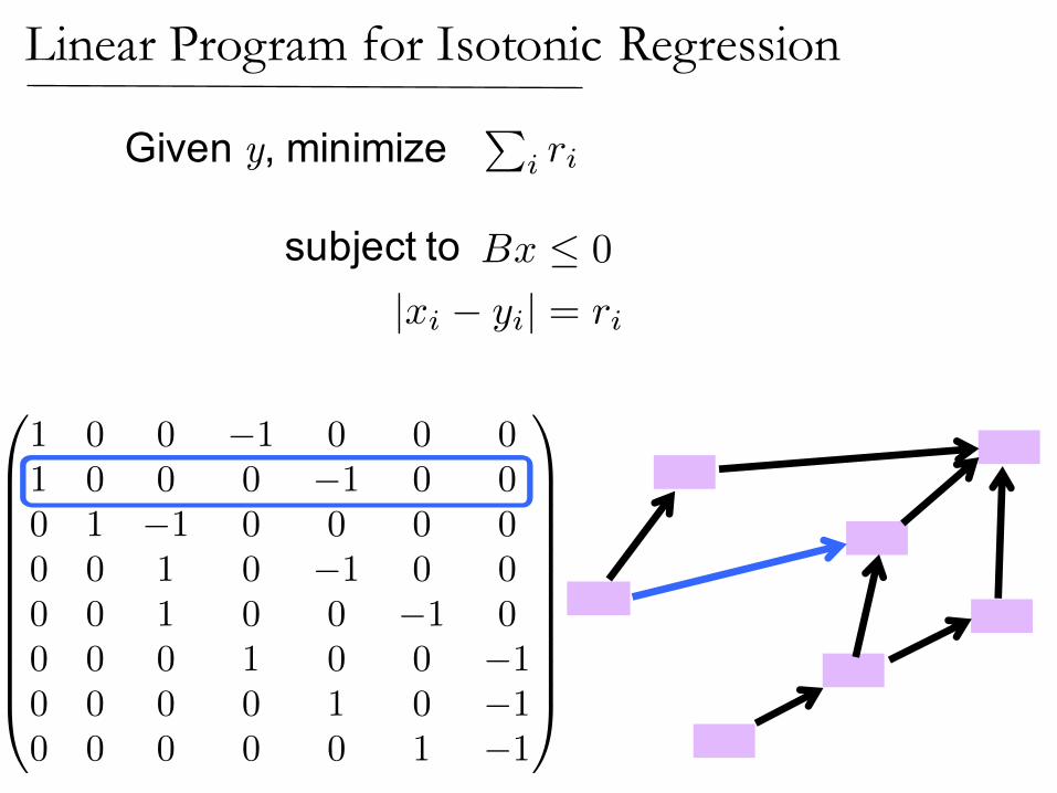
Bx 0
|xi � yi| = ri
Given y, minimize
subject to
Pi ri
B =
0
BBBBBBBBBB@
1 0 0 �1 0 0 01 0 0 0 �1 0 00 1 �1 0 0 0 00 0 1 0 �1 0 00 0 1 0 0 �1 00 0 0 1 0 0 �10 0 0 0 1 0 �10 0 0 0 0 1 �1
1
CCCCCCCCCCA
Linear Program for Isotonic Regression
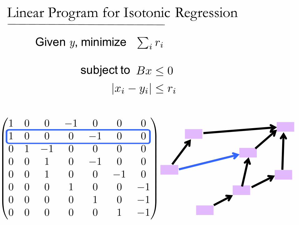
Given y, minimize
subject to
Pi ri
Bx 0
|xi � yi| ri
B =
0
BBBBBBBBBB@
1 0 0 �1 0 0 01 0 0 0 �1 0 00 1 �1 0 0 0 00 0 1 0 �1 0 00 0 1 0 0 �1 00 0 0 1 0 0 �10 0 0 0 1 0 �10 0 0 0 0 1 �1
1
CCCCCCCCCCA
Linear Program for Isotonic Regression
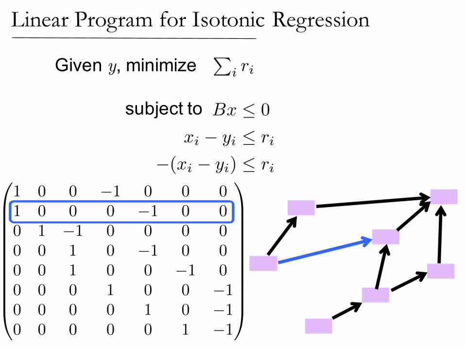
Bx 0
xi � yi ri
�(xi � yi) ri
Given y, minimize
subject to
Pi ri
B =
0
BBBBBBBBBB@
1 0 0 �1 0 0 01 0 0 0 �1 0 00 1 �1 0 0 0 00 0 1 0 �1 0 00 0 1 0 0 �1 00 0 0 1 0 0 �10 0 0 0 1 0 �10 0 0 0 0 1 �1
1
CCCCCCCCCCA
Linear Program for Isotonic Regression
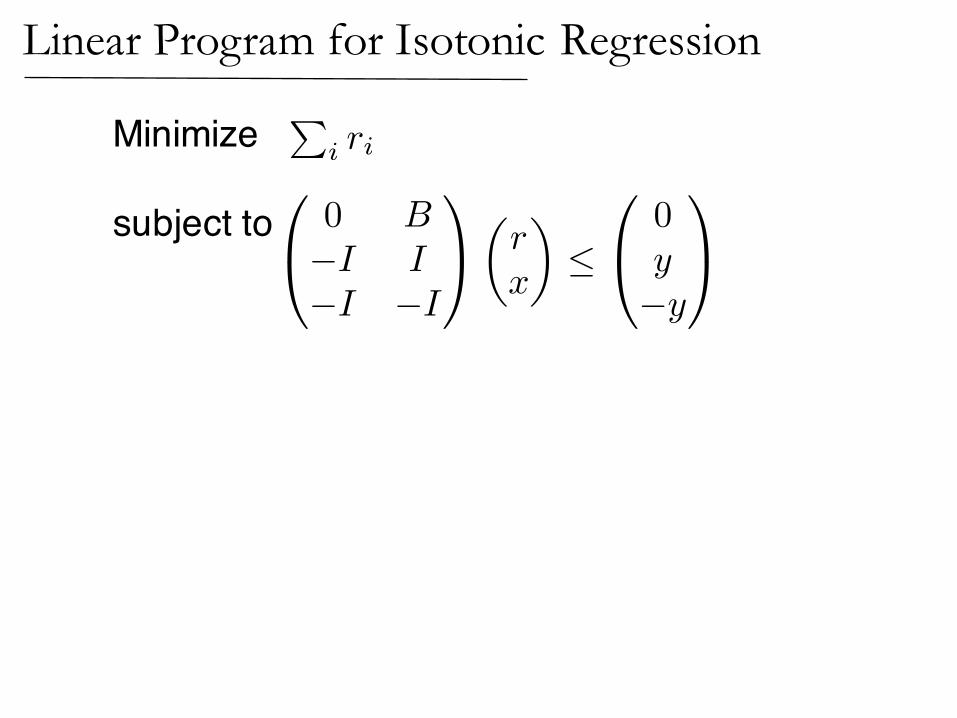
Minimize
subject to
Pi ri
0
@0 B
�I I
�I �I
1
A✓r
x
◆
0
@0y
�y
1
A
Linear Program for Isotonic Regression
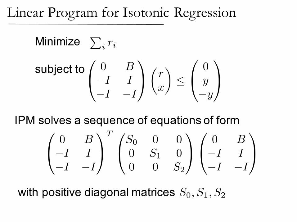
Minimize
subject to
Pi ri
0
@0 B
�I I
�I �I
1
A✓r
x
◆
0
@0y
�y
1
A
IPM solves a sequence of equations of form0
@0 B�I I�I �I
1
AT 0
@S0 0 00 S1 00 0 S2
1
A
0
@0 B�I I�I �I
1
A
with positive diagonal matrices S0, S1, S2
Linear Program for Isotonic Regression
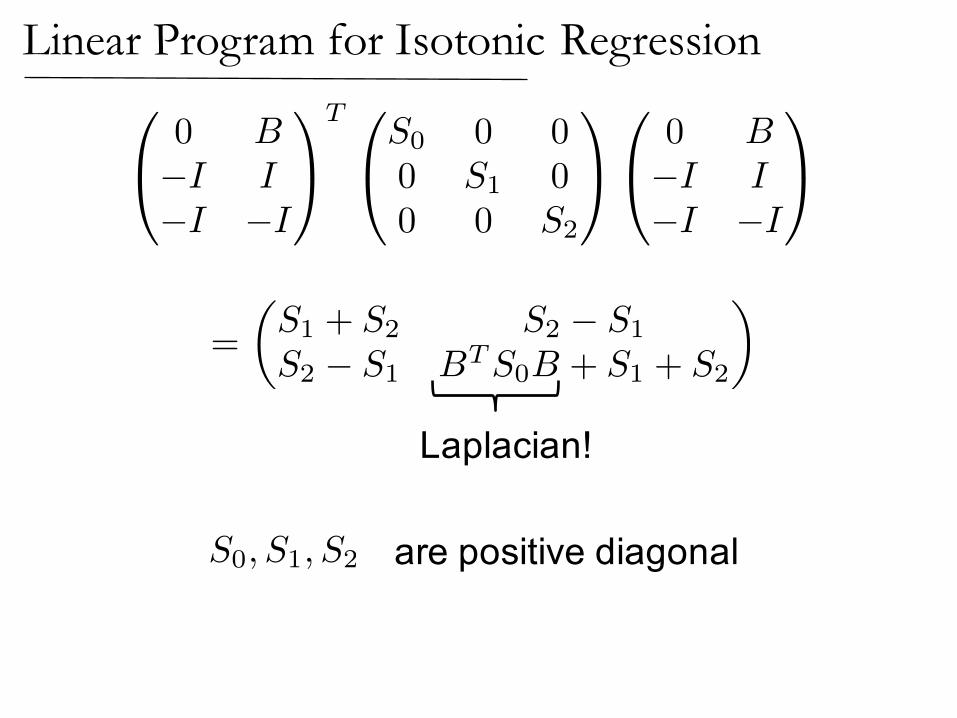
0
@0 B�I I�I �I
1
AT 0
@S0 0 00 S1 00 0 S2
1
A
0
@0 B�I I�I �I
1
A
=
✓S1 + S2 S2 � S1
S2 � S1 BTS0B + S1 + S2
◆
S0, S1, S2 are positive diagonal
Laplacian!
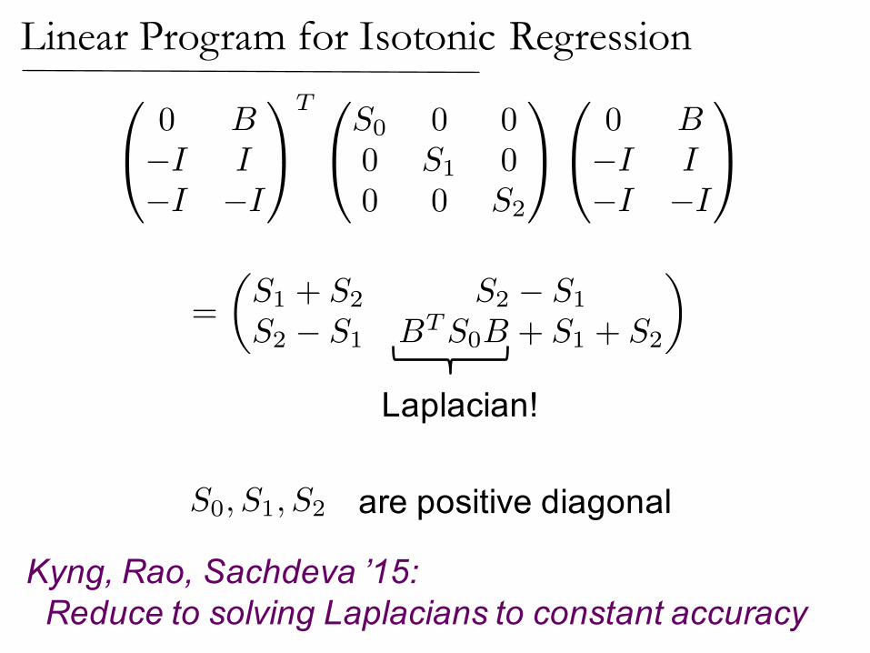
Linear Program for Isotonic Regression
0
@0 B�I I�I �I
1
AT 0
@S0 0 00 S1 00 0 S2
1
A
0
@0 B�I I�I �I
1
A
=
✓S1 + S2 S2 � S1
S2 � S1 BTS0B + S1 + S2
◆
S0, S1, S2 are positive diagonal
Laplacian!
Kyng, Rao, Sachdeva ’15: Reduce to solving Laplacians to constant accuracy
Linear Program for Isotonic Regression
Spectral Sparsification
Every graph can be approximated by a sparse graph with a similar Laplacian
for all x
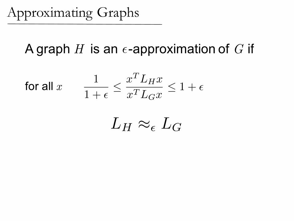
A graph H is an -approximation of G if ✏
1
1 + � xTLHx
xTLGx 1 + �
Approximating Graphs
LH ⇡✏ LG
for all x
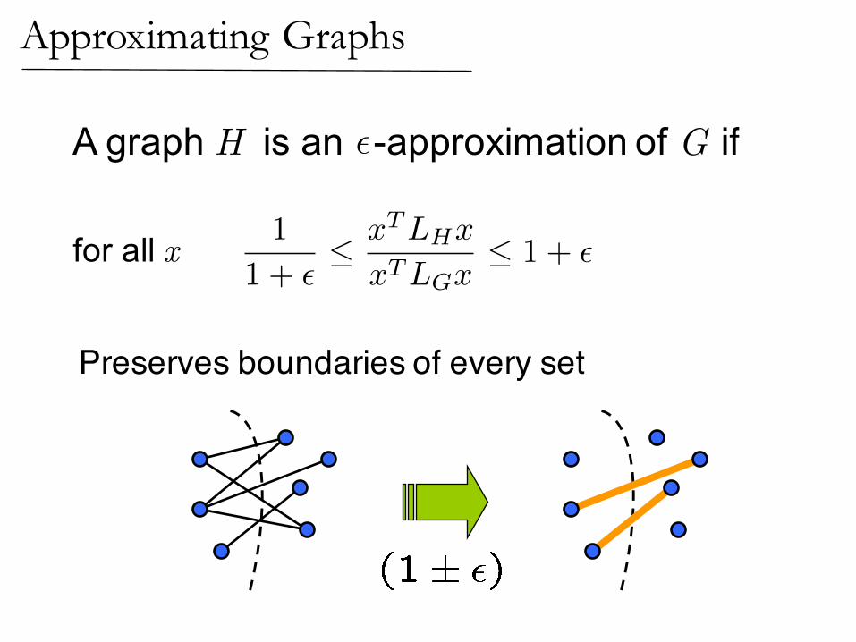
A graph H is an -approximation of G if ✏
1
1 + � xTLHx
xTLGx 1 + �
Approximating Graphs
Preserves boundaries of every set
Solutions to linear equations are similiar
for all x
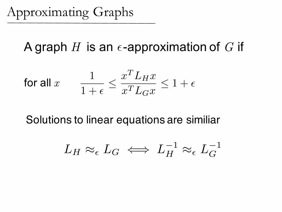
A graph H is an -approximation of G if ✏
1
1 + � xTLHx
xTLGx 1 + �
Approximating Graphs
LH ⇡✏ LG () L�1H ⇡✏ L
�1G
Spectral Sparsification
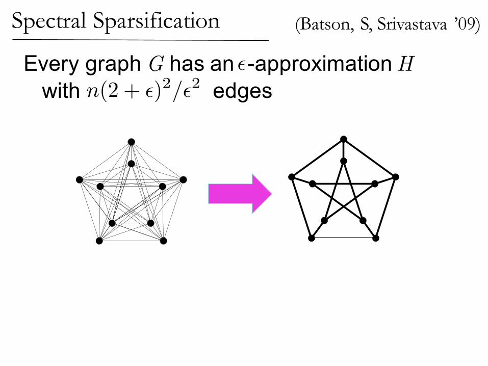
Every graph G has an -approximation Hwith edges n(2 + ✏)2/✏2
✏
(Batson, S, Srivastava ’09)

Spectral Sparsification
Every graph G has an -approximation Hwith edges n(2 + ✏)2/✏2
✏
(Batson, S, Srivastava ’09)
Random regular graphs approximate complete graphs
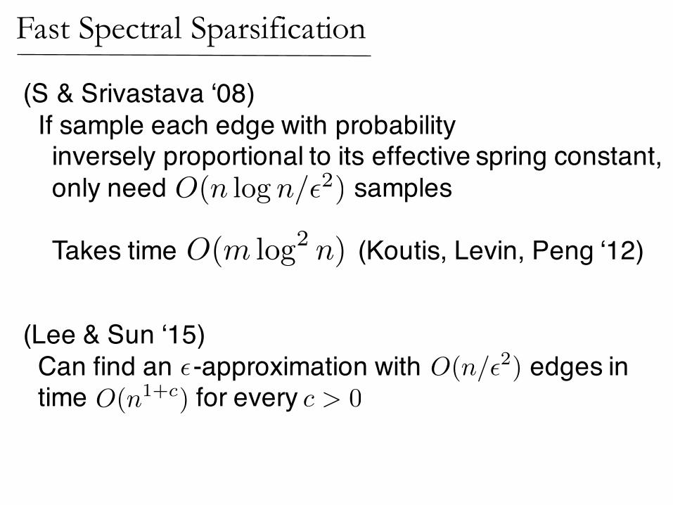
Fast Spectral Sparsification
(S & Srivastava ‘08) If sample each edge with probability inversely proportional to its effective spring constant,only need samples
Takes time (Koutis, Levin, Peng ‘12)
O(n log n/✏2)
(Lee & Sun ‘15) Can find an -approximation with edges in time for every
O(n/✏2)✏O(n1+c) c > 0
O(m log
2 n)
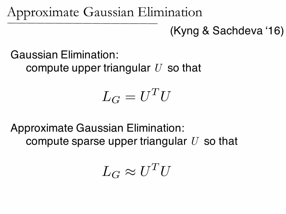
(Kyng & Sachdeva ‘16)Approximate Gaussian Elimination
Gaussian Elimination:compute upper triangular U so that
LG = UTU
Approximate Gaussian Elimination:compute sparse upper triangular U so that
LG ⇡ UTU

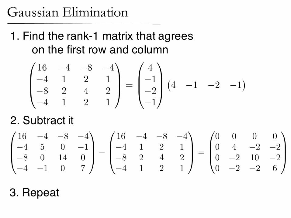
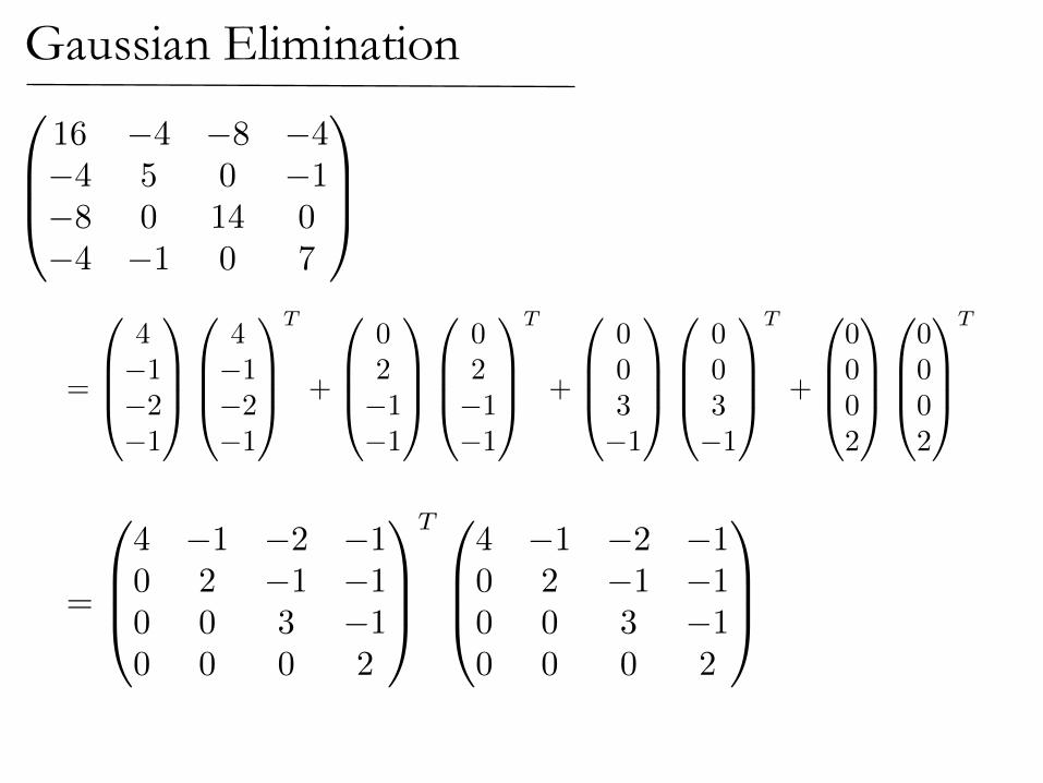
Gaussian Elimination
1. Find the rank-1 matrix that agrees on the first row and column
2. Subtract it
0
BB@
16 �4 �8 �4�4 5 0 �1�8 0 14 0�4 �1 0 7
1
CCA
0
BB@
16 �4 �8 �4�4 1 2 1�8 2 4 2�4 1 2 1
1
CCA =
0
BB@
4�1�2�1
1
CCA�4 �1 �2 �1
�
Gaussian Elimination1. Find the rank-1 matrix that agrees
on the first row and column
2. Subtract it
0
BB@
16 �4 �8 �4�4 1 2 1�8 2 4 2�4 1 2 1
1
CCA =
0
BB@
4�1�2�1
1
CCA�4 �1 �2 �1
�
0
BB@
16 �4 �8 �4�4 5 0 �1�8 0 14 0�4 �1 0 7
1
CCA�
0
BB@
16 �4 �8 �4�4 1 2 1�8 2 4 2�4 1 2 1
1
CCA =
0
BB@
0 0 0 00 4 �2 �20 �2 10 �20 �2 �2 6
1
CCA
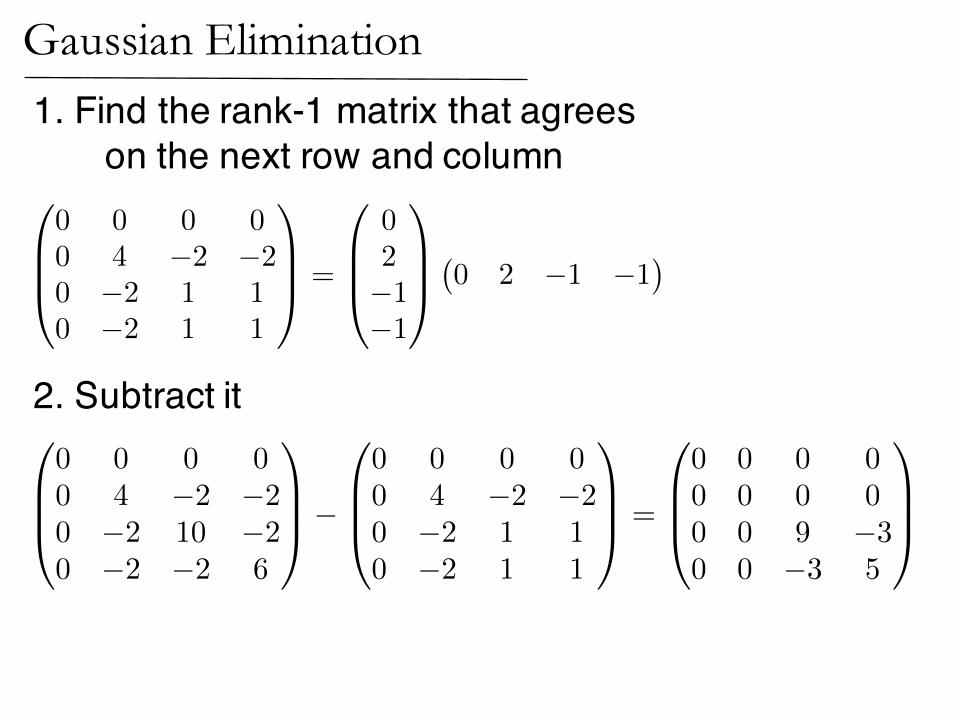
3. Repeat
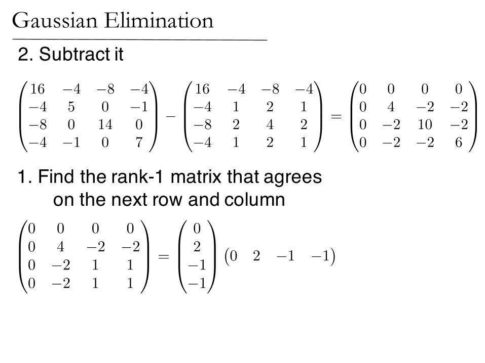
Gaussian Elimination
1. Find the rank-1 matrix that agrees on the next row and column
2. Subtract it0
BB@
16 �4 �8 �4�4 5 0 �1�8 0 14 0�4 �1 0 7
1
CCA�
0
BB@
16 �4 �8 �4�4 1 2 1�8 2 4 2�4 1 2 1
1
CCA =
0
BB@
0 0 0 00 4 �2 �20 �2 10 �20 �2 �2 6
1
CCA
0
BB@
0 0 0 00 4 �2 �20 �2 1 10 �2 1 1
1
CCA =
0
BB@
02�1�1
1
CCA�0 2 �1 �1
�
Gaussian Elimination1. Find the rank-1 matrix that agrees
on the next row and column
2. Subtract it
0
BB@
0 0 0 00 4 �2 �20 �2 1 10 �2 1 1
1
CCA =
0
BB@
02�1�1
1
CCA�0 2 �1 �1
�
0
BB@
0 0 0 00 4 �2 �20 �2 10 �20 �2 �2 6
1
CCA�
0
BB@
0 0 0 00 4 �2 �20 �2 1 10 �2 1 1
1
CCA =
0
BB@
0 0 0 00 0 0 00 0 9 �30 0 �3 5
1
CCA
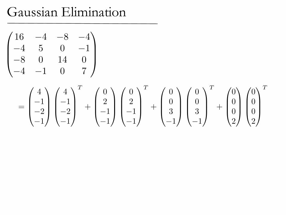
Gaussian Elimination
=
0
BB@
4�1�2�1
1
CCA
0
BB@
4�1�2�1
1
CCA
T
+
0
BB@
02�1�1
1
CCA
0
BB@
02�1�1
1
CCA
T
+
0
BB@
003�1
1
CCA
0
BB@
003�1
1
CCA
T
+
0
BB@
0002
1
CCA
0
BB@
0002
1
CCA
T
0
BB@
16 �4 �8 �4�4 5 0 �1�8 0 14 0�4 �1 0 7
1
CCA
Gaussian Elimination
=
0
BB@
4�1�2�1
1
CCA
0
BB@
4�1�2�1
1
CCA
T
+
0
BB@
02�1�1
1
CCA
0
BB@
02�1�1
1
CCA
T
+
0
BB@
003�1
1
CCA
0
BB@
003�1
1
CCA
T
+
0
BB@
0002
1
CCA
0
BB@
0002
1
CCA
T
0
BB@
16 �4 �8 �4�4 5 0 �1�8 0 14 0�4 �1 0 7
1
CCA
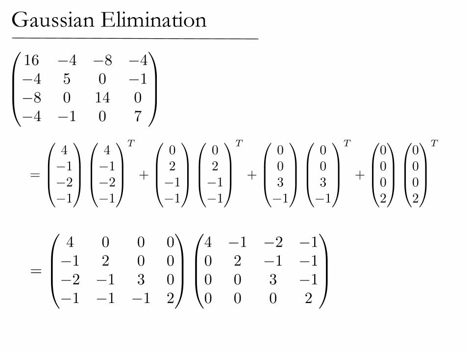
=
0
BB@
4 0 0 0�1 2 0 0�2 �1 3 0�1 �1 �1 2
1
CCA
0
BB@
4 �1 �2 �10 2 �1 �10 0 3 �10 0 0 2
1
CCA
Gaussian Elimination
=
0
BB@
4�1�2�1
1
CCA
0
BB@
4�1�2�1
1
CCA
T
+
0
BB@
02�1�1
1
CCA
0
BB@
02�1�1
1
CCA
T
+
0
BB@
003�1
1
CCA
0
BB@
003�1
1
CCA
T
+
0
BB@
0002
1
CCA
0
BB@
0002
1
CCA
T
0
BB@
16 �4 �8 �4�4 5 0 �1�8 0 14 0�4 �1 0 7
1
CCA
=
0
BB@
4 �1 �2 �10 2 �1 �10 0 3 �10 0 0 2
1
CCA
T 0
BB@
4 �1 �2 �10 2 �1 �10 0 3 �10 0 0 2
1
CCA
Gaussian Elimination
=
0
BB@
4�1�2�1
1
CCA
0
BB@
4�1�2�1
1
CCA
T
+
0
BB@
02�1�1
1
CCA
0
BB@
02�1�1
1
CCA
T
+
0
BB@
003�1
1
CCA
0
BB@
003�1
1
CCA
T
+
0
BB@
0002
1
CCA
0
BB@
0002
1
CCA
T
0
BB@
16 �4 �8 �4�4 5 0 �1�8 0 14 0�4 �1 0 7
1
CCA
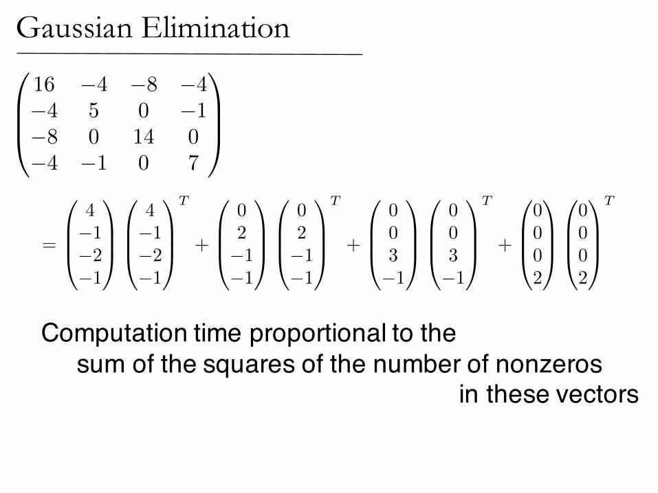
Computation time proportional to the sum of the squares of the number of nonzeros
in these vectors
Gaussian Elimination of Laplacians
0
BB@
16 �4 �8 �4�4 5 0 �1�8 0 14 0�4 �1 0 7
1
CCA�
0
BB@
4�1�2�1
1
CCA
0
BB@
4�1�2�1
1
CCA
T
=
0
BB@
0 0 0 00 4 �2 �20 �2 10 �20 �2 �2 6
1
CCA
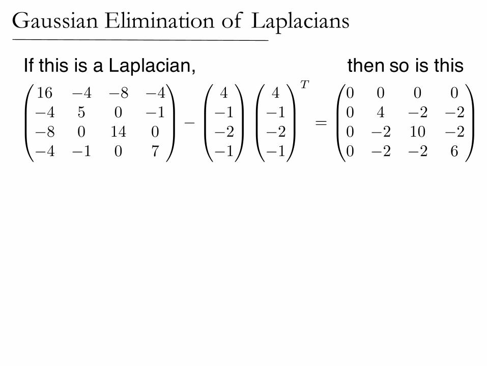
If this is a Laplacian, then so is this
0
BB@
16 �4 �8 �4�4 5 0 �1�8 0 14 0�4 �1 0 7
1
CCA�
0
BB@
4�1�2�1
1
CCA
0
BB@
4�1�2�1
1
CCA
T
=
0
BB@
0 0 0 00 4 �2 �20 �2 10 �20 �2 �2 6
1
CCA
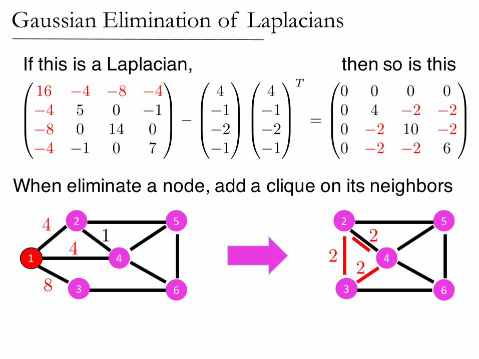
Gaussian Elimination of Laplacians
If this is a Laplacian, then so is this
2
1 4
3 6
54
8
4 12
4
3 6
5
222
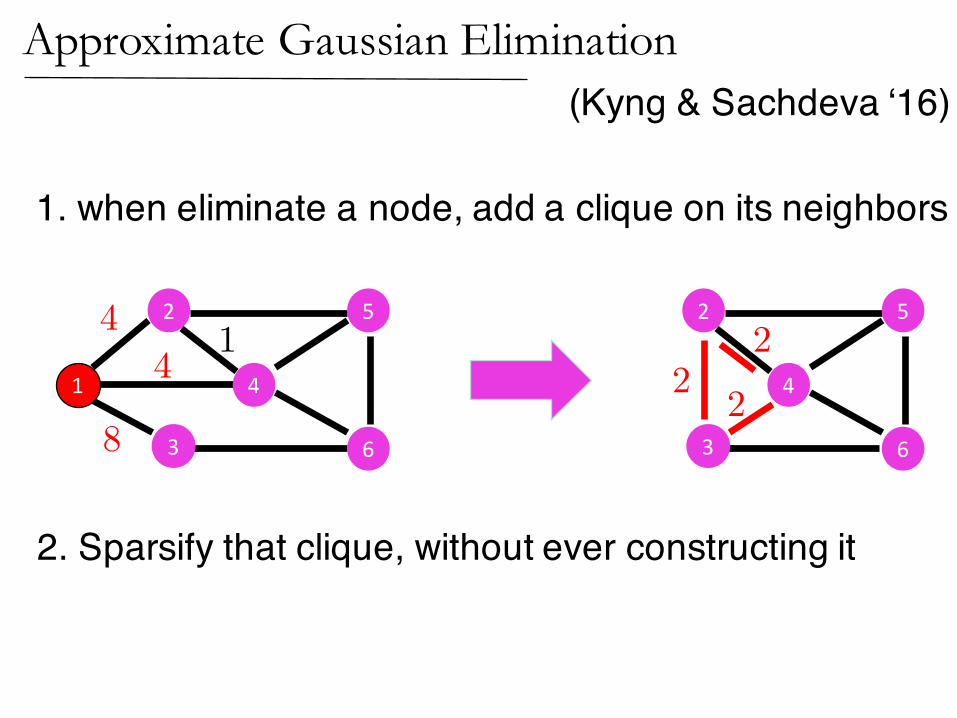
When eliminate a node, add a clique on its neighbors
Approximate Gaussian Elimination
2
1 4
3 6
54
8
4 12
4
3 6
5
222
1. when eliminate a node, add a clique on its neighbors
2. Sparsify that clique, without ever constructing it
(Kyng & Sachdeva ‘16)
(Kyng & Sachdeva ‘16)Approximate Gaussian Elimination
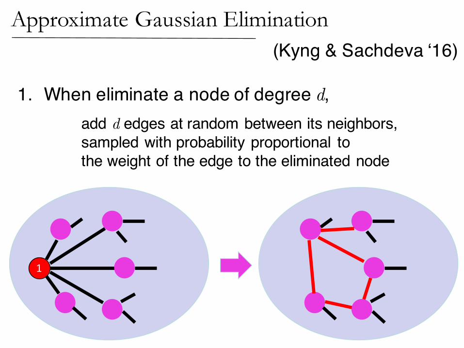
1. When eliminate a node of degree d,add d edges at random between its neighbors, sampled with probability proportional to the weight of the edge to the eliminated node
1
(Kyng & Sachdeva ‘16)Approximate Gaussian Elimination
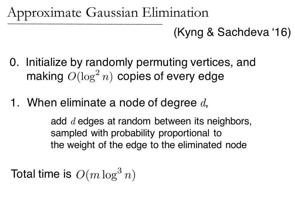
0. Initialize by randomly permuting vertices, and making copies of every edgeO(log
2 n)
1. When eliminate a node of degree d,add d edges at random between its neighbors, sampled with probability proportional to the weight of the edge to the eliminated node
Total time is O(m log
3 n)
(Kyng & Sachdeva ‘16)Approximate Gaussian Elimination
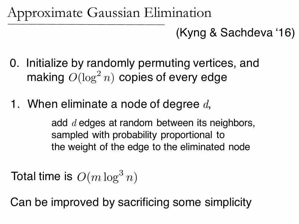
0. Initialize by randomly permuting vertices, and making copies of every edgeO(log
2 n)
Total time is O(m log
3 n)
1. When eliminate a node of degree d,add d edges at random between its neighbors, sampled with probability proportional to the weight of the edge to the eliminated node
Can be improved by sacrificing some simplicity
(Kyng & Sachdeva ‘16)Approximate Gaussian Elimination
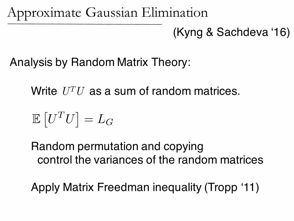
Analysis by Random Matrix Theory:
Write UTU as a sum of random matrices.
Random permutation and copying control the variances of the random matrices
Apply Matrix Freedman inequality (Tropp ‘11)
E⇥UTU
⇤= LG
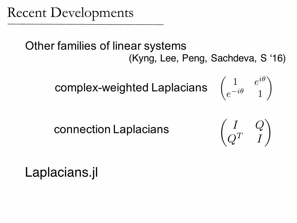
Other families of linear systems
complex-weighted Laplacians
connection Laplacians
✓1 ei✓
e�i✓ 1
◆
✓I QQT I
◆
Recent Developments
(Kyng, Lee, Peng, Sachdeva, S ‘16)
Laplacians.jl
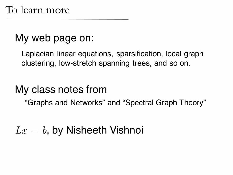
To learn more
My web page on:Laplacian linear equations, sparsification, local graph clustering, low-stretch spanning trees, and so on.
My class notes from “Graphs and Networks” and “Spectral Graph Theory”
Lx = b, by Nisheeth Vishnoi


![Spectral distributions of adjacency and Laplacian matrices ...users.stat.umn.edu/~jiang040/papers/Adj_Markov5.pdf · routing in graphs, one can see [15]. Although there are many matrices](https://img.dokumen.tips/doc/110x75/5fc5c36ad951d42aad3d1c2f/spectral-distributions-of-adjacency-and-laplacian-matrices-usersstatumnedujiang040papersadj.jpg)