Knot Theory For Spatial Graphs Attached To A Surfacekawauchi/KnotTheoryforSpatial...Knot Theory For Spatial Graphs Attached To A Surface Akio Kawauchi Abstract. Beside a survey on

Knot Theory For Spatial Graphs Attached To A Surface

Akio Kawauchi

Abstract. Beside a survey on several unknotting notions of a spatial graphdone earlier by the author, unknotting notions on a spatial graph with degreeone vertices attached to a surface are introduced.

1. Introduction

In the ICTS program KNOT-2013 given at the Indian Institute of ScienceEducation and Research (IISER) Mohali, the author delivered the following threelectures:

[Lecture 1] Topology for spatial graphs without degree one vertices

[Lecture 2] Unknotting notions on the spatial graphs

[Lecture 3] Spatial graphs with degree one vertices attaching to a surface

Topics on the first two lectures come from the author’s earlier papers [17, 18]whose overview is also explained in this article. Topics on the third lecture aremotivated to know knotting structures of a model tying two objects with differentscales, or more concretely to understand knotting structures on a spatial graphwhose degree one vertices are attached to a surface. For example, one asks thefollowing question:

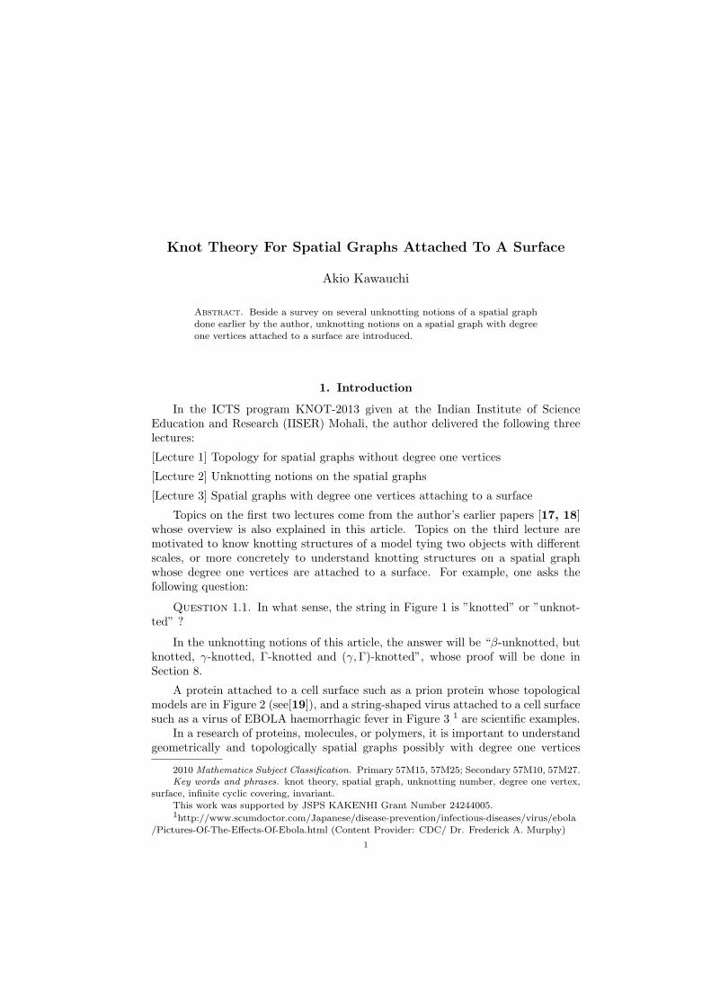
Question 1.1. In what sense, the string in Figure 1 is ”knotted” or ”unknot-ted” ?

In the unknotting notions of this article, the answer will be “β-unknotted, butknotted, γ-knotted, Γ-knotted and (γ,Γ)-knotted”, whose proof will be done inSection 8.

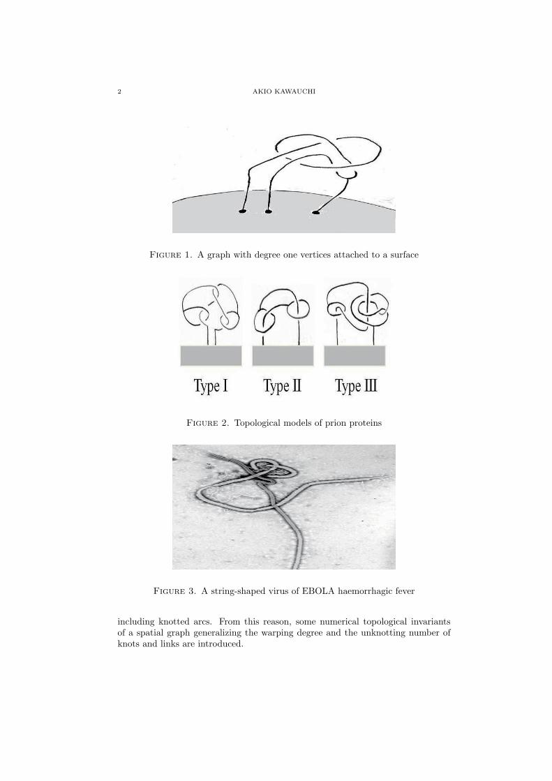
A protein attached to a cell surface such as a prion protein whose topologicalmodels are in Figure 2 (see[19]), and a string-shaped virus attached to a cell surfacesuch as a virus of EBOLA haemorrhagic fever in Figure 3 1 are scientific examples.

In a research of proteins, molecules, or polymers, it is important to understandgeometrically and topologically spatial graphs possibly with degree one vertices

2010 Mathematics Subject Classification. Primary 57M15, 57M25; Secondary 57M10, 57M27.Key words and phrases. knot theory, spatial graph, unknotting number, degree one vertex,

surface, infinite cyclic covering, invariant.This work was supported by JSPS KAKENHI Grant Number 24244005.1http://www.scumdoctor.com/Japanese/disease-prevention/infectious-diseases/virus/ebola

/Pictures-Of-The-Effects-Of-Ebola.html (Content Provider: CDC/ Dr. Frederick A. Murphy)

1

2 AKIO KAWAUCHI

Figure 1. A graph with degree one vertices attached to a surface

Figure 2. Topological models of prion proteins

Figure 3. A string-shaped virus of EBOLA haemorrhagic fever

including knotted arcs. From this reason, some numerical topological invariantsof a spatial graph generalizing the warping degree and the unknotting number ofknots and links are introduced.

SPATIAL GRAPHS ATTACHED TO A SURFACE 3

In Section 2, the equivalence of a spatial graph without degree one vertices isexplained. In Section 3, a monotone diagram, the warping degree, the complexityand the cross-index for a spatial graph without degree one vertices are explained.In Section 4, an unknotted graph and the induced unknotting number are explainedfor a spatial graph without degree one vertices and for a spatial graph with degreeone vertices attaching to a surface. In Section 5, a β-unknotted graph and theinduced unknotting number are explained for a spatial graph without degree onevertices and for a spatial graph with degree one vertices attaching to a surface. InSection 6, a homological invariant of an infinite cyclic covering of a spatial graphis discussed to estimate the β-unknotting number. In Section 7, a γ-unknottedgraph and the induced unknotting number are explained for a spatial graph withoutdegree one vertices and for a spatial graph with degree one vertices attaching to asurface. In Section 8, a Γ-unknotted graph and the induced unknotting number areexplained for a spatial graph without degree one vertices and for a spatial graphwith degree one vertices attaching to a surface. In Section 9, the values taken bythese unknotting numbers are investigated. In Section 10, a notion of the knottingprobability of a spatial graph with degree one free vertices is explained.

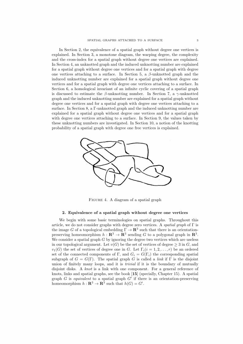
Figure 4. A diagram of a spatial graph

2. Equivalence of a spatial graph without degree one vertices

We begin with some basic terminologies on spatial graphs. Throughout thisarticle, we do not consider graphs with degree zero vertices. A spatial graph of Γ isthe image G of a topological embedding Γ → R3 such that there is an orientation-preserving homeomorphism h : R3 → R3 sending G to a polygonal graph in R3.We consider a spatial graph G by ignoring the degree two vertices which are uselessin our topological argument. Let v(G) be the set of vertices of degree ≥ 3 in G, andv1(G) the set of vertices of degree one in G. Let Γi(i = 1, 2, . . . , r) be an orderedset of the connected components of Γ, and Gi = G(Γi) the corresponding spatialsubgraph of G = G(Γ). The spatial graph G is called a link if Γ is the disjointunion of finitely many loops, and it is trivial if it is the boundary of mutuallydisjoint disks. A knot is a link with one component. For a general reference ofknots, links and spatial graphs, see the book [15] (specially, Chapter 15). A spatialgraph G is equivalent to a spatial graph G′ if there is an orientation-preservinghomeomorphism h : R3 → R3 such that h(G) = G′.

4 AKIO KAWAUCHI

For a spatial graph G with v1(G) = ∅, let [G] be the class of spatial graphs G′

which are equivalent to G. A diagram DG of a spatial graph G with v1(G) = ∅ inR3 is an the image of G into a plane P under an orthogonal projection

proj : R3 → P

with only double point singularities on edges of G together with the upper-lowercrossing information (see Figure 4).

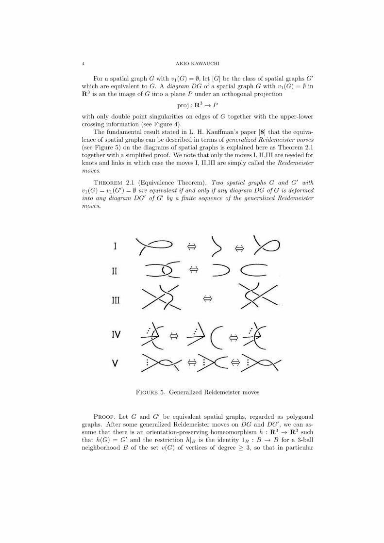
The fundamental result stated in L. H. Kauffman’s paper [8] that the equiva-lence of spatial graphs can be described in terms of generalized Reidemeister moves(see Figure 5) on the diagrams of spatial graphs is explained here as Theorem 2.1together with a simplified proof. We note that only the moves I, II,III are needed forknots and links in which case the moves I, II,III are simply called the Reidemeistermoves.

Theorem 2.1 (Equivalence Theorem). Two spatial graphs G and G′ withv1(G) = v1(G

′) = ∅ are equivalent if and only if any diagram DG of G is deformedinto any diagram DG′ of G′ by a finite sequence of the generalized Reidemeistermoves.　　

　

Figure 5. Generalized Reidemeister moves

Proof. Let G and G′ be equivalent spatial graphs, regarded as polygonalgraphs. After some generalized Reidemeister moves on DG and DG′, we can as-sume that there is an orientation-preserving homeomorphism h : R3 → R3 suchthat h(G) = G′ and the restriction h|B is the identity 1B : B → B for a 3-ballneighborhood B of the set v(G) of vertices of degree ≥ 3, so that in particular


we have v(G) = v(G′). Thus, there is a one-parameter family of piecewise-linearhomeomorphisms

ht : R3 → R3 (0 ≤ t ≤ 1)

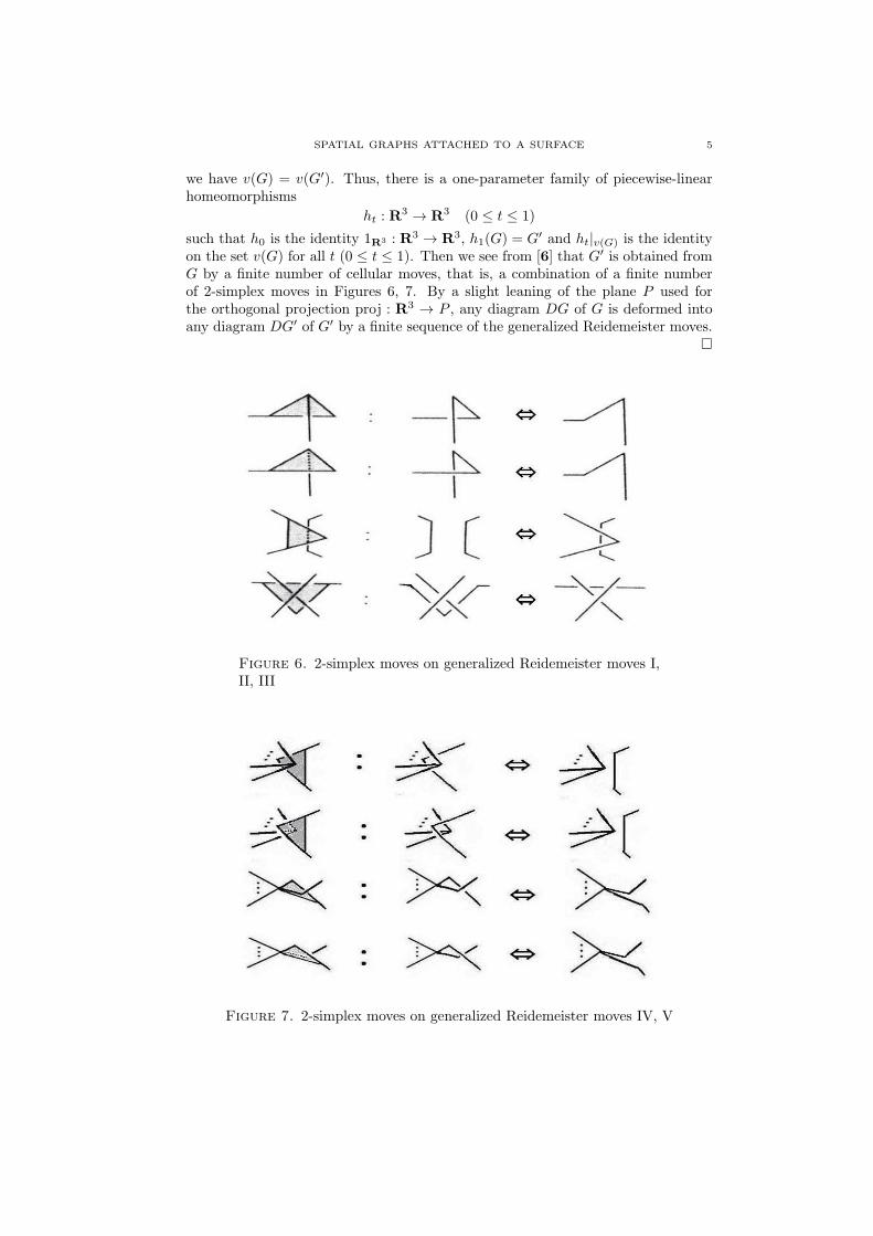
such that h0 is the identity 1R3 : R3 → R3, h1(G) = G′ and ht|v(G) is the identityon the set v(G) for all t (0 ≤ t ≤ 1). Then we see from [6] that G′ is obtained fromG by a finite number of cellular moves, that is, a combination of a finite numberof 2-simplex moves in Figures 6, 7. By a slight leaning of the plane P used forthe orthogonal projection proj : R3 → P , any diagram DG of G is deformed intoany diagram DG′ of G′ by a finite sequence of the generalized Reidemeister moves.　 □

Figure 6. 2-simplex moves on generalized Reidemeister moves I,II, III

Figure 7. 2-simplex moves on generalized Reidemeister moves IV, V

6 AKIO KAWAUCHI

Let [DG] be the class of diagrams obtained from a diagram DG of a spatialgraph G with v1(G) = ∅ by the generalized Reidemeister moves, which is identifiedwith the class [G] by the equivalence theorem. The fundamental topological prob-lems on spatial graphs are stated as follows, which are natural generalizations ofthe fundamental problems of knot theory:

(1) Study what kinds of spatial graphs there are. List them up to equivalences.

(2) Determine whether two given spatial graphs of a graph Γ are equivalent or not.

A basic question on the relationship between a spatial graph and knot theoryis to ask how a spatial graph is related to knot theory. A constituent knot (or aconstituent link, resp.) of a spatial graph G is a knot (or link, resp.) contained inG. The following proposition is direct from the definition of equivalence.

Proposition 2.2. If two spatial graphs G∗ and G are equivalent, then thereis a graph-isomorphism f : G∗ → G such that every constituent knot or link L∗ ofG∗ is equivalent to the corresponding constituent knot or link f(L∗) of G.

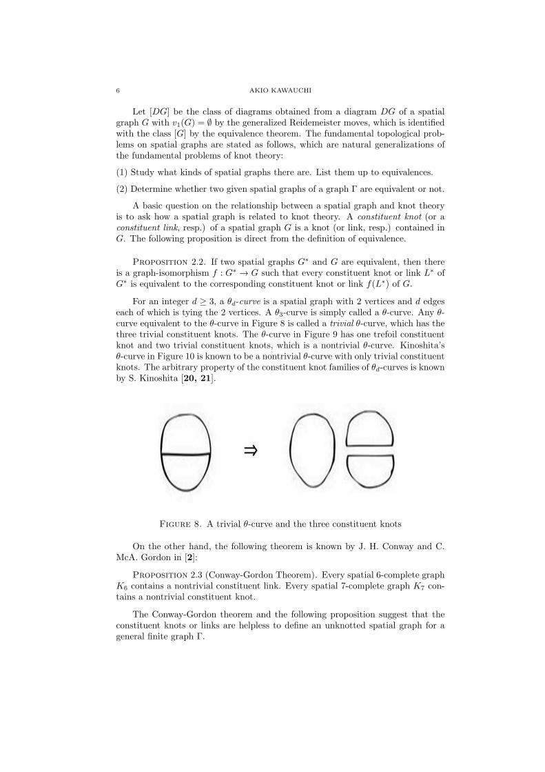
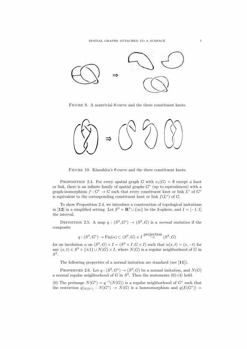
For an integer d ≥ 3, a θd-curve is a spatial graph with 2 vertices and d edgeseach of which is tying the 2 vertices. A θ3-curve is simply called a θ-curve. Any θ-curve equivalent to the θ-curve in Figure 8 is called a trivial θ-curve, which has thethree trivial constituent knots. The θ-curve in Figure 9 has one trefoil constituentknot and two trivial constituent knots, which is a nontrivial θ-curve. Kinoshita’sθ-curve in Figure 10 is known to be a nontrivial θ-curve with only trivial constituentknots. The arbitrary property of the constituent knot families of θd-curves is knownby S. Kinoshita [20, 21].

Figure 8. A trivial θ-curve and the three constituent knots

On the other hand, the following theorem is known by J. H. Conway and C.McA. Gordon in [2]:

Proposition 2.3 (Conway-Gordon Theorem). Every spatial 6-complete graphK6 contains a nontrivial constituent link. Every spatial 7-complete graph K7 con-tains a nontrivial constituent knot.

The Conway-Gordon theorem and the following proposition suggest that theconstituent knots or links are helpless to define an unknotted spatial graph for ageneral finite graph Γ.


Figure 9. A nontrivial θ-curve and the three constituent knots

Figure 10. Kinoshita’s θ-curve and the three constituent knots

Proposition 2.4. For every spatial graph G with v1(G) = ∅ except a knotor link, there is an infinite family of spatial graphs G∗ (up to equivalences) with agraph-isomorphism f : G∗ → G such that every constituent knot or link L∗ of G∗

is equivalent to the corresponding constituent knot or link f(L∗) of G.

To show Proposition 2.4, we introduce a construction of topological imitationsin [12] in a simplified setting. Let S3 = R3 ∪ {∞} be the 3-sphere, and I = [−1, 1]the interval.

Definition 2.5. A map q : (S3, G∗) → (S3, G) is a normal imitation if thecomposite

q : (S3, G∗) → Fix(α) ⊂ (S3, G)× Iprojection→ (S3, G)

for an involution α on (S3, G)× I = (S3 × I,G× I) such that α(x, t) = (x,−t) forany (x, t) ∈ S3 × {±1} ∪N(G)× I, where N(G) is a regular neighborhood of G inS3.

The following properties of a normal imitation are standard (see [11]).

Properties 2.6. Let q : (S3, G∗) → (S3, G) be a normal imitation, and N(G)a normal regular neighborhood of G in S3. Then the statements (0)-(4) hold.

(0) The preimage N(G∗) = q−1(N(G)) is a regular neighborhood of G∗ such thatthe restriction q|N(G∗) : N(G∗) → N(G) is a homeomorphism and q(E(G∗)) =

8 AKIO KAWAUCHI

E(G) for the exteriors E(G∗) = cl(S3\N(G∗)) and E(G) = cl(S3\N(G)) of thespatial graphs G∗ and G, respectively.

(1) The map q1 : (S3, G∗1) → (S3, G1) defined by q for any spatial graph G1 in

N(G) and G∗1 = q−1(G1) is a normal imitation.

(2) We have the same linking number LinkS3(L∗) = LinkS3(L) for any oriented2-component links L in N(G) and L∗ = q−1(L).

(3) The homomorphism q# : π1(S3\G∗) → π1(S

3\G) on fundamental group is anepimorphism whose kernel Ker(q#) is a perfact group, i.e.,

Ker(q#) = [Ker(q#),Ker(q#)].

(4) For normal imitations q : (S3, G∗) → (S3, G) and q∗ : (S3, G∗∗) → (S3, G∗),there is a normal imitation q∗∗ : (S3, G∗∗) → (S3, G).

The Kinoshita-Terasaka knot is an example of a normal imitation of a triv-ial knot (see [11]). We say that a normal imitation q : (S3, G∗) → (S3, G) ishomotopy-trivial if there is a 1-parameter family {qs}0≤s≤1 of normal imitationsqs : (S3, G∗) → (S3, G) such that q0 = q and q1 is a homeomorphism. The fol-lowing notion is useful in constructing several nontrivial knots, links and spatialgraphs.

Definition 2.7. A normal imitation q : (S3, G∗) → (S3, G) is an AID imitationif the restriction

q|(S3,cl(G∗\α∗)) : (S

3, cl(G∗\α∗)) → (S3, cl(G\α))

is homotopy-trivial for every pair of an edge α of G and an edge α∗ of G∗ withq(α∗) = α.

The following proposition is a main result on the existence of AID imitationsin [12].

Proposition 2.8. For any spatial graph G with v1(G) = ∅, there is an infinitefamily of AID imitations q : (S3, G∗) → (S3, G) such that the fundamental groupsπ1(E(G∗)) of the exteriors E(G∗) of the spatial graphs G∗ with v1(G

∗) = ∅ aremutually non-isomorphic.

Proposition 2.4 is a direct consequence of Proposition 2.8. Further, combiningProposition 2.8 with a result in [13], we can add an additional property that everyspatial graph G∗ is obtained from G by one crossing change.

3. A monotone diagram, the warping degree, the complexity and thecross-index for a spatial graph without degree one vertices

Let Gi (i = 1, 2, . . . , r) be the connected components of a spatial graph Gwith v1(G) = ∅. Let Ti be a maximal tree of Gi. By definition, Ti = ∅ if Gi isa knot, and Ti is one vertex if Gi has just one vertex of degree ≥ 3. The unionT = ∪r

i=1Ti is called a basis of G, and the pair (G,T ) a based spatial graph. Thespatial graph G is obtained from a basis T by adding edges (consisting of arcs orloops) αk (k = 1, 2, . . . ,m). Let D be a diagram of G. Let DT and Dαk be thesubdiagrams of D corresponding to the basis T and the edge αk, respectively. Thediagram D is a based diagram on a basis T and denoted by (D;T ) if there are no


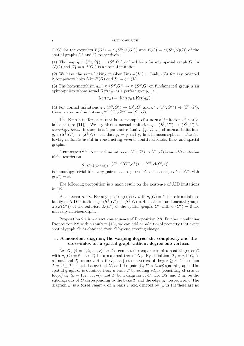
Figure 11. Deforming the diagram of Figure 4 into a based diagram

crossing points of D belonging to DT . Every diagram can be deformed into a baseddiagram by a finite sequence of the generalized Reidemeister moves (see Figure 11).

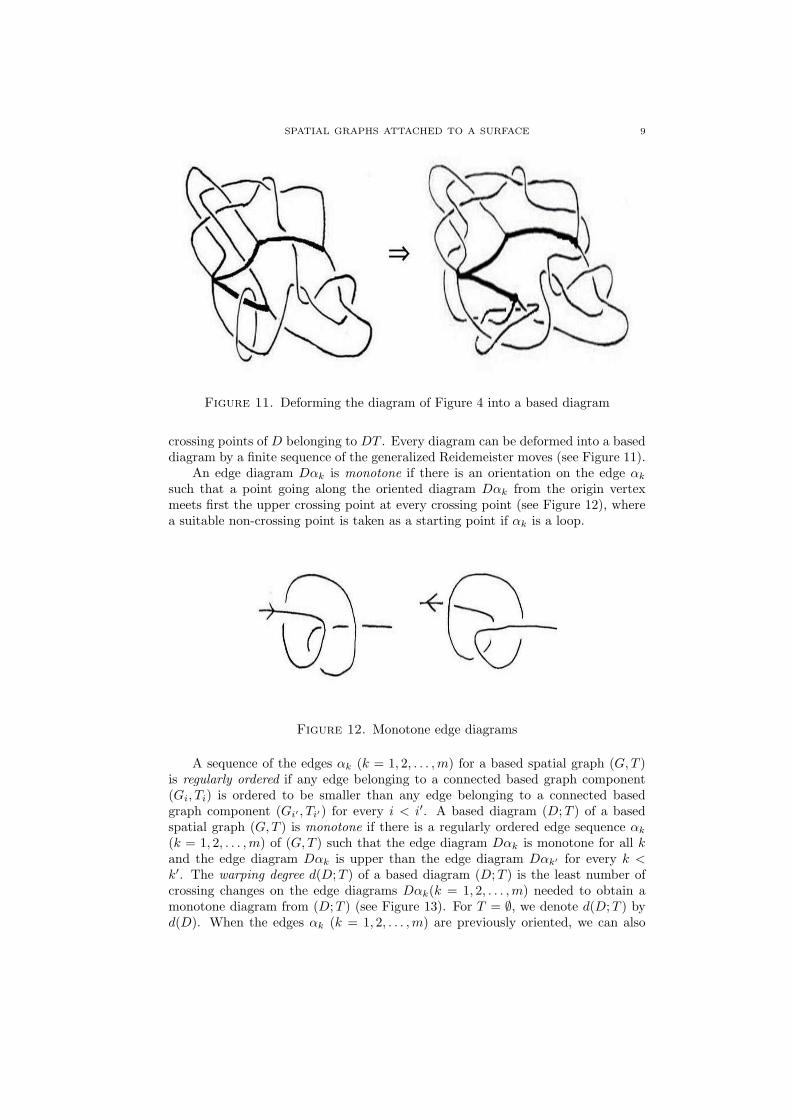
An edge diagram Dαk is monotone if there is an orientation on the edge αk

such that a point going along the oriented diagram Dαk from the origin vertexmeets first the upper crossing point at every crossing point (see Figure 12), wherea suitable non-crossing point is taken as a starting point if αk is a loop.

Figure 12. Monotone edge diagrams

A sequence of the edges αk (k = 1, 2, . . . ,m) for a based spatial graph (G,T )is regularly ordered if any edge belonging to a connected based graph component(Gi, Ti) is ordered to be smaller than any edge belonging to a connected basedgraph component (Gi′ , Ti′) for every i < i′. A based diagram (D;T ) of a basedspatial graph (G,T ) is monotone if there is a regularly ordered edge sequence αk

(k = 1, 2, . . . ,m) of (G,T ) such that the edge diagram Dαk is monotone for all kand the edge diagram Dαk is upper than the edge diagram Dαk′ for every k <k′. The warping degree d(D;T ) of a based diagram (D;T ) is the least number ofcrossing changes on the edge diagrams Dαk(k = 1, 2, . . . ,m) needed to obtain amonotone diagram from (D;T ) (see Figure 13). For T = ∅, we denote d(D;T ) byd(D). When the edges αk (k = 1, 2, . . . ,m) are previously oriented, we can also

10 AKIO KAWAUCHI

define the oriented warping degree d(D;T ) (or d(D) for T = ∅) of a based diagram(D;T ) by considering only the crossing changes on the edge or loop diagrams Dαk

(k = 1, 2, . . . ,m) along the specified orientations. Similar notions on links havebeen discussed by W. B. R. Lickorish and K. C. Millett [22], S. Fujimura [4], T. S.Fung [5], M. Okuda [26] and M. Ozawa [27] considering the ascending number ofan oriented link. A. Shimizu [29, 30] also established a relationship between thewarping degrees and the crossing number of a knot or link diagram. In particular, A.Shimizu characterized the alternating knot diagrams by establishing the inequality

d(D) + d(−D) ≤ c(D)− 1

for every knot diagram D with crossing number c(D) > 0, where the equality holdsif and only if D is an alternating diagram. For the present applications, we notethe following relationships

d(Dα) + d(−Dα) = c(Dα), d(Dα) = min{d(Dα), d(−Dα)}for an oriented edge diagram Dα and the oppositely oriented edge diagram −Dα,where c(Dα) denotes the crossing number of D(α). For example,

d

( )= 1,

for

d

( )= 1 and d

( )= 3.

The warping degree d(G) of a spatial graph G with v1(G) = ∅ is the minimum ofthe warping degrees d(D;T ) for all based diagrams (D;T ) ∈ [DG]. The complexityof a based diagram (D,T ) is the pair cd(D;T ) = (c(D;T ), d(D;T )) together withthe dictionary order. This notion was introduced in [16] for an oriented ordered linkdiagram. A. Shimizu observed that the dictionary order on cd(D;T ) is equivalent tothe numerical order on c(D;T )2+d(D;T ) by using the inequality d(D;T ) ≤ c(D;T ).

The complexity of a spatial graph G with v1(G) = ∅ is the minimum γ(G) =(cγ(G), dγ(G)) (in the dictionary order) of the complexities cd(D;T ) for all baseddiagrams (D;T ) ∈ [DG], where the topological invariants cγ(G) and dγ(G) arecalled the γ-crossing number and the γ-warping degree of G, respectively.

The crossing number of a spatial graph G with v1(G) = ∅ is a non-negativeinteger given by c(G) = minD∈[DG] c(D). By definition, we have the inequality

c(G) ≤ cγ(G).

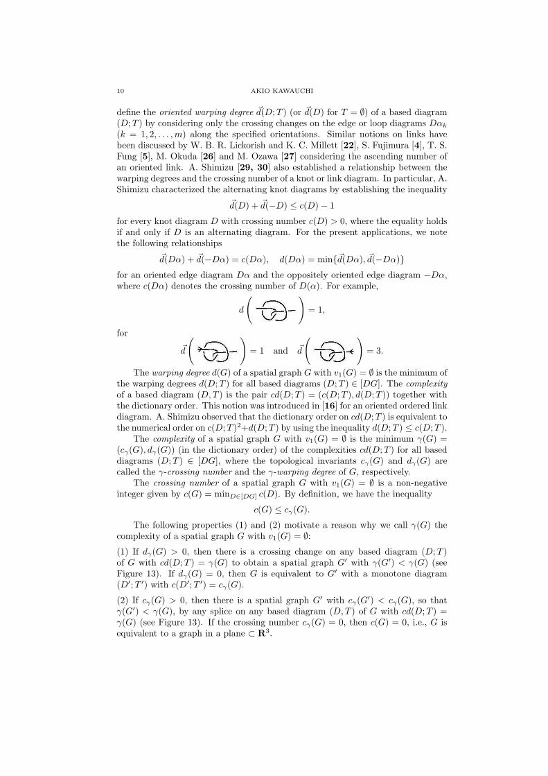
The following properties (1) and (2) motivate a reason why we call γ(G) thecomplexity of a spatial graph G with v1(G) = ∅:(1) If dγ(G) > 0, then there is a crossing change on any based diagram (D;T )of G with cd(D;T ) = γ(G) to obtain a spatial graph G′ with γ(G′) < γ(G) (seeFigure 13). If dγ(G) = 0, then G is equivalent to G′ with a monotone diagram(D′;T ′) with c(D′;T ′) = cγ(G).

(2) If cγ(G) > 0, then there is a spatial graph G′ with cγ(G′) < cγ(G), so that

γ(G′) < γ(G), by any splice on any based diagram (D,T ) of G with cd(D;T ) =γ(G) (see Figure 13). If the crossing number cγ(G) = 0, then c(G) = 0, i.e., G isequivalent to a graph in a plane ⊂ R3.


Figure 13. A crossing change in the left hand side and a splicein the right hand side

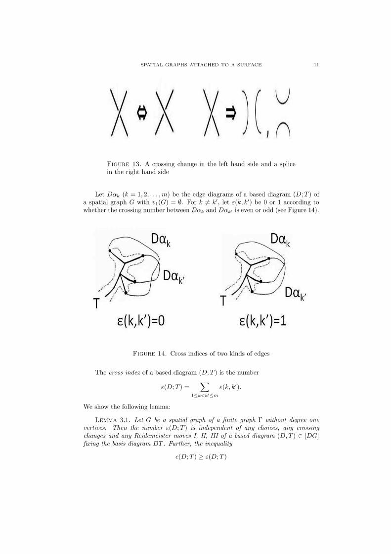
Let Dαk (k = 1, 2, . . . ,m) be the edge diagrams of a based diagram (D;T ) ofa spatial graph G with v1(G) = ∅. For k = k′, let ε(k, k′) be 0 or 1 according towhether the crossing number between Dαk and Dαk′ is even or odd (see Figure 14).

Figure 14. Cross indices of two kinds of edges

The cross index of a based diagram (D;T ) is the number

ε(D;T ) =∑

1≤k<k′≤m

ε(k, k′).

We show the following lemma:

Lemma 3.1. Let G be a spatial graph of a finite graph Γ without degree onevertices. Then the number ε(D;T ) is independent of any choices, any crossingchanges and any Reidemeister moves I, II, III of a based diagram (D,T ) ∈ [DG]fixing the basis diagram DT . Further, the inequality

c(D;T ) ≥ ε(D;T )

12 AKIO KAWAUCHI

holds and there is a spatial graph G∗ of the finite graph Γ with a based diagram(D∗;T ) ∈ [DG∗] with the same basis T such that

c(D∗;T ) = ε(D∗;T ) = ε(D;T ).

Proof. By definition, we have c(D;T ) ≥ ε(D;T ). By crossing changes andReidemeister moves, we can reduce the number c(D;T ) to attain the numberε(D;T ). □

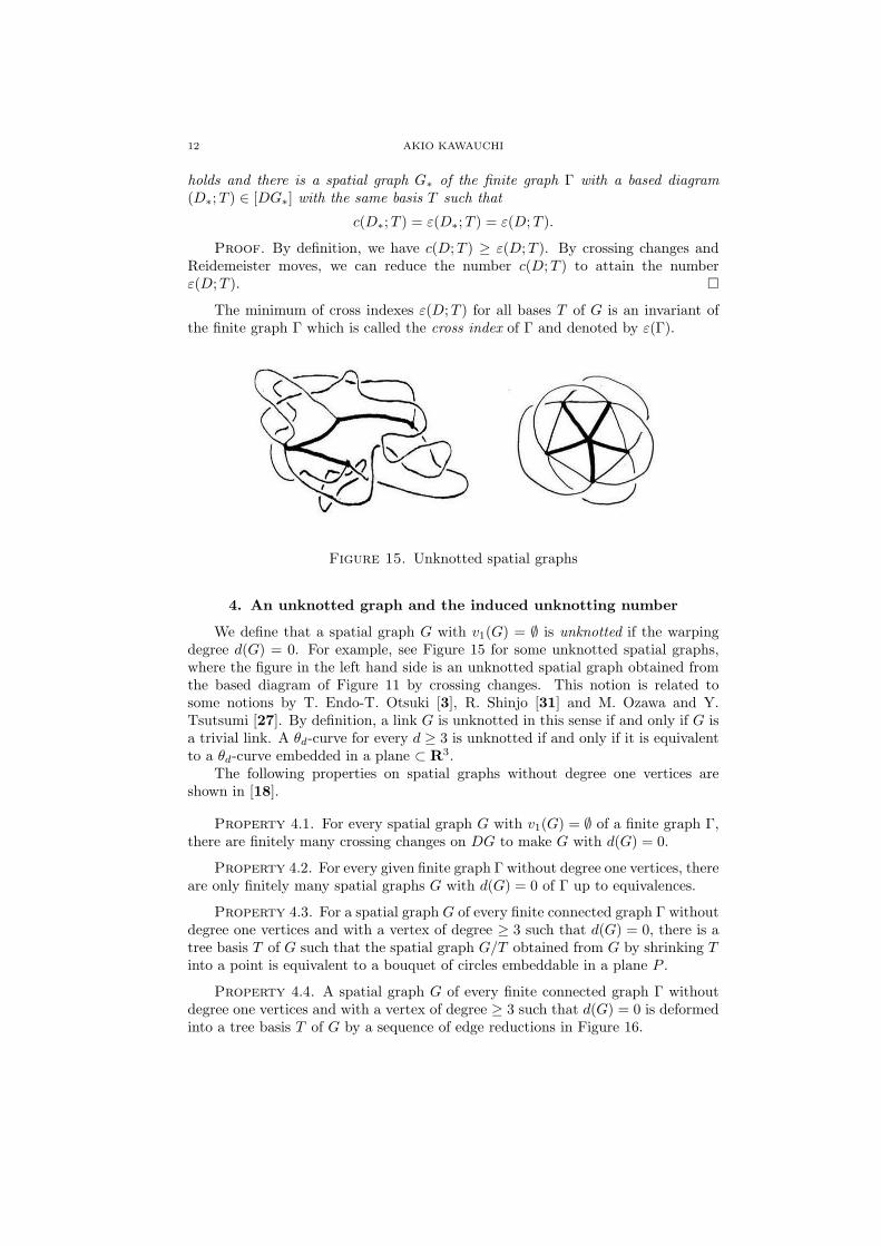
The minimum of cross indexes ε(D;T ) for all bases T of G is an invariant ofthe finite graph Γ which is called the cross index of Γ and denoted by ε(Γ).

Figure 15. Unknotted spatial graphs

4. An unknotted graph and the induced unknotting number

We define that a spatial graph G with v1(G) = ∅ is unknotted if the warpingdegree d(G) = 0. For example, see Figure 15 for some unknotted spatial graphs,where the figure in the left hand side is an unknotted spatial graph obtained fromthe based diagram of Figure 11 by crossing changes. This notion is related tosome notions by T. Endo-T. Otsuki [3], R. Shinjo [31] and M. Ozawa and Y.Tsutsumi [27]. By definition, a link G is unknotted in this sense if and only if G isa trivial link. A θd-curve for every d ≥ 3 is unknotted if and only if it is equivalentto a θd-curve embedded in a plane ⊂ R3.

The following properties on spatial graphs without degree one vertices areshown in [18].

Property 4.1. For every spatial graph G with v1(G) = ∅ of a finite graph Γ,there are finitely many crossing changes on DG to make G with d(G) = 0.

Property 4.2. For every given finite graph Γ without degree one vertices, thereare only finitely many spatial graphs G with d(G) = 0 of Γ up to equivalences.

Property 4.3. For a spatial graph G of every finite connected graph Γ withoutdegree one vertices and with a vertex of degree ≥ 3 such that d(G) = 0, there is atree basis T of G such that the spatial graph G/T obtained from G by shrinking Tinto a point is equivalent to a bouquet of circles embeddable in a plane P .

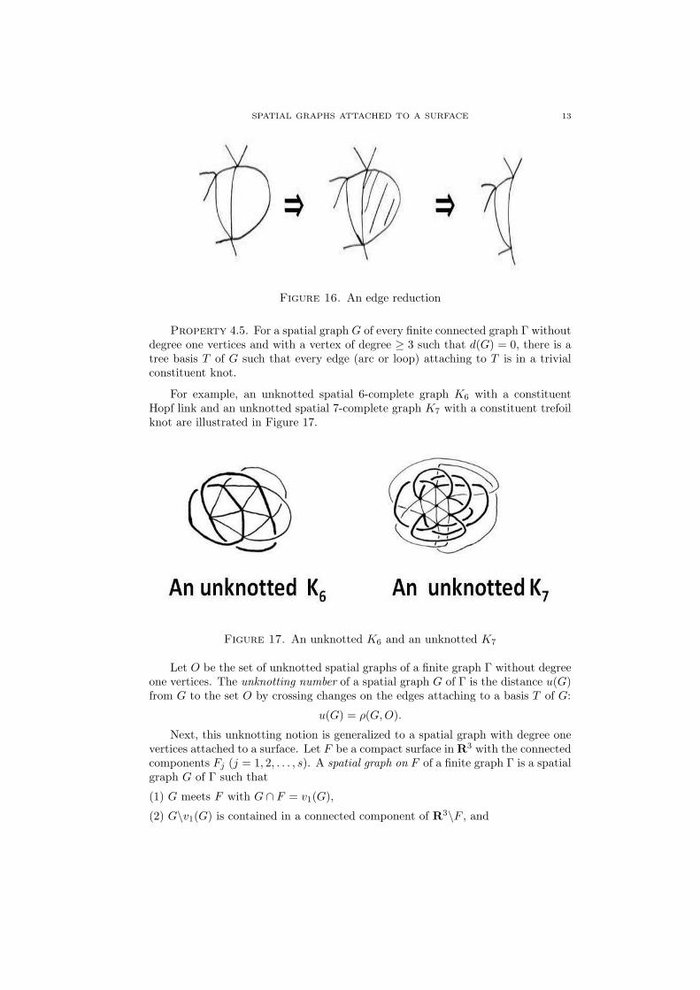
Property 4.4. A spatial graph G of every finite connected graph Γ withoutdegree one vertices and with a vertex of degree ≥ 3 such that d(G) = 0 is deformedinto a tree basis T of G by a sequence of edge reductions in Figure 16.


Figure 16. An edge reduction

Property 4.5. For a spatial graph G of every finite connected graph Γ withoutdegree one vertices and with a vertex of degree ≥ 3 such that d(G) = 0, there is atree basis T of G such that every edge (arc or loop) attaching to T is in a trivialconstituent knot.

For example, an unknotted spatial 6-complete graph K6 with a constituentHopf link and an unknotted spatial 7-complete graph K7 with a constituent trefoilknot are illustrated in Figure 17.

Figure 17. An unknotted K6 and an unknotted K7

Let O be the set of unknotted spatial graphs of a finite graph Γ without degreeone vertices. The unknotting number of a spatial graph G of Γ is the distance u(G)from G to the set O by crossing changes on the edges attaching to a basis T of G:

u(G) = ρ(G,O).

Next, this unknotting notion is generalized to a spatial graph with degree onevertices attached to a surface. Let F be a compact surface in R3 with the connectedcomponents Fj (j = 1, 2, . . . , s). A spatial graph on F of a finite graph Γ is a spatialgraph G of Γ such that

(1) G meets F with G ∩ F = v1(G),

(2) G\v1(G) is contained in a connected component of R3\F , and

14 AKIO KAWAUCHI

(3) there is a homeomorphism h : R3 → R3 such that h(G ∪ F ) is a compactpolyhedron in R3.

Further, we impose the following mild conditions (4)-(5) on the spatial graphG and the surface F :

(4) F does not need ∂F = ∅.

(5) Although we grant that Γ, G or F are disconnected, assume that |Fj∩v1(G)| ≥ 2for every j.

A spatial graph G on a surface F is equivalent to a spatial graph G′ on asurface F ′ if there is an orientation-preserving homeomorphism h : R3 → R3 suchthat h(F ∪G) = F ′∪G′. A shrinked spatial graph of a spatial graph G on a surface

F is a spatial graph G with v1(G) = ∅ in R3 obtained from G by shrinking a 2-cell∆j with

Fj ⊃ ∆j ⊃ Fj ∩ V1(G)

into a point for every j. We put the following definition.

Definition 4.6. A spatial graph G on a surface F is unknotted if there is anunknotted shrinked spatial graph G of G.

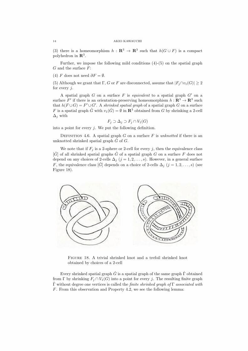
We note that if Fj is a 2-sphere or 2-cell for every j, then the equivalence class

[G] of all shrinked spatial graphs G of a spatial graph G on a surface F does notdepend on any choices of 2-cells ∆j (j = 1, 2, . . . , s). However, in a general surface

F , the equivalence class [G] depends on a choice of 2-cells ∆j (j = 1, 2, . . . , s) (seeFigure 18).

Figure 18. A trivial shrinked knot and a trefoil shrinked knotobtained by choices of a 2-cell

Every shrinked spatial graph G is a spatial graph of the same graph Γ obtainedfrom Γ by shrinking Fj ∩ V1(G) into a point for every j. The resulting finite graph

Γ without degree one vertices is called the finite shrinked graph of Γ associated withF . From this observation and Property 4.2, we see the following lemma:


Lemma 4.7. For any given finite graph Γ with degree one vertices and any givensurface F in R3, there are only finitely many unknotted spatial graphs G of Γ onthe surface F up to equivalences.

Let OF be the set of unknotted spatial graphs of a finite graph Γ on a surfaceF . The unknotting number of a spatial graph G of a finite graph Γ on a surface Fis the distance u(G) from the set {G} of all shrinked spatial graphs G to the setOF by crossing changes on the edges attaching to a basis:

u(G) = ρ({G}, OF ).

5. A β-unknotted graph and the induced unknotting number

Let G be a spatial graph G with v1(G) = ∅, and T a basis of G with Ti

(i = 1, 2, . . . , r) the connected components. Let B be the disjoint union of mutuallydisjoint 3-ball regular neighborhoods Bi of Ti in S3 (i = 1, 2, . . . , r). Let Bc =cl(S3\B) be the complement domain of B, and L = Bc ∩G be an m-string tanglein Bc consisting of mutually disjoint m arcs which is called the complementarytangle of the based graph (G,T ). We put the following definition.

Definition 5.1. A spatial graph G with v1(G) = ∅ is β-unknotted if there is abasis T of G whose complementary tangle (Bc, L) is trivial, meaning that L is in acompact punctured 2-sphere properly embedded in Bc.

Here are some observations on β-unknotted spatial graphs.

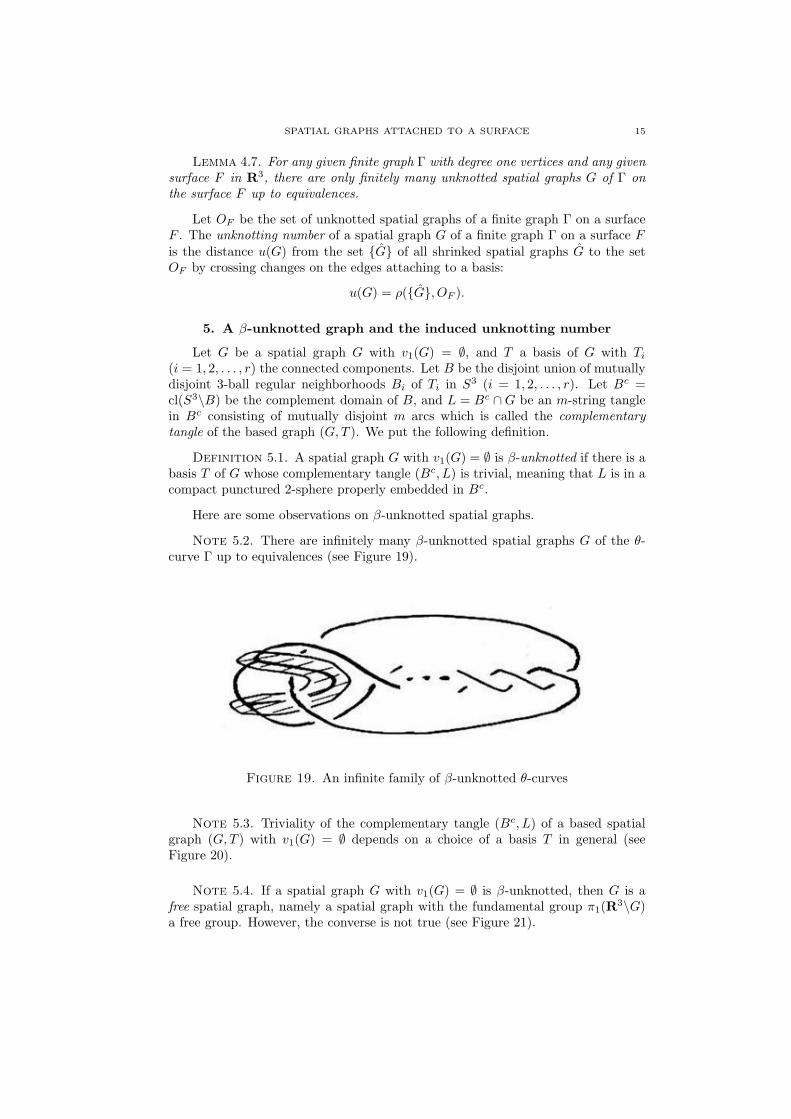
Note 5.2. There are infinitely many β-unknotted spatial graphs G of the θ-curve Γ up to equivalences (see Figure 19).

Figure 19. An infinite family of β-unknotted θ-curves

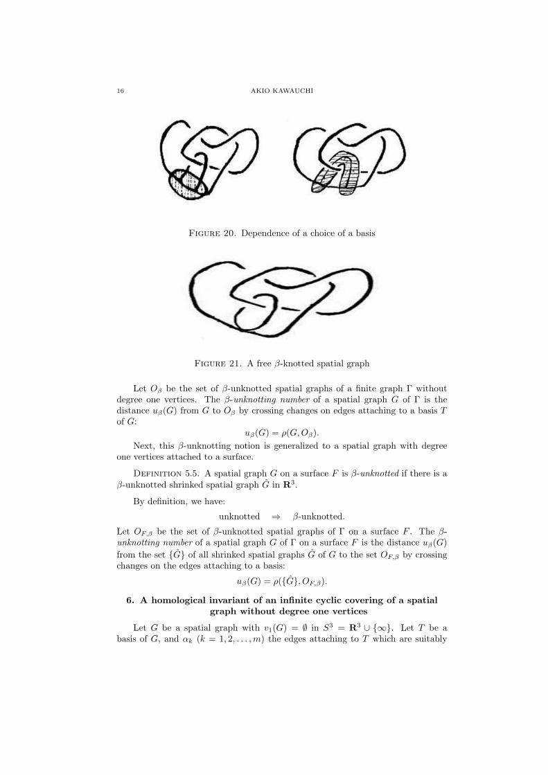
Note 5.3. Triviality of the complementary tangle (Bc, L) of a based spatialgraph (G,T ) with v1(G) = ∅ depends on a choice of a basis T in general (seeFigure 20).

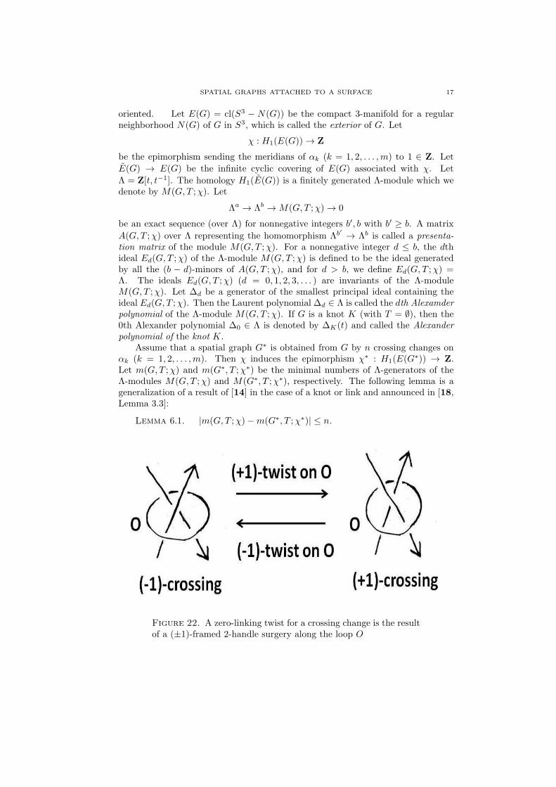
Note 5.4. If a spatial graph G with v1(G) = ∅ is β-unknotted, then G is afree spatial graph, namely a spatial graph with the fundamental group π1(R

3\G)a free group. However, the converse is not true (see Figure 21).

16 AKIO KAWAUCHI

Figure 20. Dependence of a choice of a basis

Figure 21. A free β-knotted spatial graph

Let Oβ be the set of β-unknotted spatial graphs of a finite graph Γ withoutdegree one vertices. The β-unknotting number of a spatial graph G of Γ is thedistance uβ(G) from G to Oβ by crossing changes on edges attaching to a basis Tof G:

uβ(G) = ρ(G,Oβ).

Next, this β-unknotting notion is generalized to a spatial graph with degreeone vertices attached to a surface.

Definition 5.5. A spatial graph G on a surface F is β-unknotted if there is aβ-unknotted shrinked spatial graph G in R3.

By definition, we have:

unknotted ⇒ β-unknotted.

Let OF,β be the set of β-unknotted spatial graphs of Γ on a surface F . The β-unknotting number of a spatial graph G of Γ on a surface F is the distance uβ(G)

from the set {G} of all shrinked spatial graphs G of G to the set OF,β by crossingchanges on the edges attaching to a basis:

uβ(G) = ρ({G}, OF,β).

6. A homological invariant of an infinite cyclic covering of a spatialgraph without degree one vertices

Let G be a spatial graph with v1(G) = ∅ in S3 = R3 ∪ {∞}. Let T be abasis of G, and αk (k = 1, 2, . . . ,m) the edges attaching to T which are suitably


oriented. 　 Let E(G) = cl(S3 − N(G)) be the compact 3-manifold for a regularneighborhood N(G) of G in S3, which is called the exterior of G. Let

χ : H1(E(G)) → Z

be the epimorphism sending the meridians of αk (k = 1, 2, . . . ,m) to 1 ∈ Z. Let

E(G) → E(G) be the infinite cyclic covering of E(G) associated with χ. Let

Λ = Z[t, t−1]. The homology H1(E(G)) is a finitely generated Λ-module which wedenote by M(G,T ;χ). Let

Λa → Λb → M(G,T ;χ) → 0

be an exact sequence (over Λ) for nonnegative integers b′, b with b′ ≥ b. A matrix

A(G,T ;χ) over Λ representing the homomorphism Λb′ → Λb is called a presenta-tion matrix of the module M(G,T ;χ). For a nonnegative integer d ≤ b, the dthideal Ed(G,T ;χ) of the Λ-module M(G,T ;χ) is defined to be the ideal generatedby all the (b − d)-minors of A(G,T ;χ), and for d > b, we define Ed(G,T ;χ) =Λ. The ideals Ed(G,T ;χ) (d = 0, 1, 2, 3, . . . ) are invariants of the Λ-moduleM(G,T ;χ). Let ∆d be a generator of the smallest principal ideal containing theideal Ed(G,T ;χ). Then the Laurent polynomial ∆d ∈ Λ is called the dth Alexamderpolynomial of the Λ-module M(G,T ;χ). If G is a knot K (with T = ∅), then the0th Alexander polynomial ∆0 ∈ Λ is denoted by ∆K(t) and called the Alexanderpolynomial of the knot K.

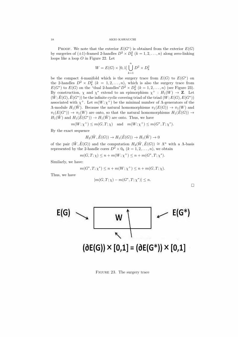
Assume that a spatial graph G∗ is obtained from G by n crossing changes onαk (k = 1, 2, . . . ,m). Then χ induces the epimorphism χ∗ : H1(E(G∗)) → Z.Let m(G,T ;χ) and m(G∗, T ;χ∗) be the minimal numbers of Λ-generators of theΛ-modules M(G,T ;χ) and M(G∗, T ;χ∗), respectively. The following lemma is ageneralization of a result of [14] in the case of a knot or link and announced in [18,Lemma 3.3]:

Lemma 6.1. |m(G,T ;χ)−m(G∗, T ;χ∗)| ≤ n.

Figure 22. A zero-linking twist for a crossing change is the resultof a (±1)-framed 2-handle surgery along the loop O

18 AKIO KAWAUCHI

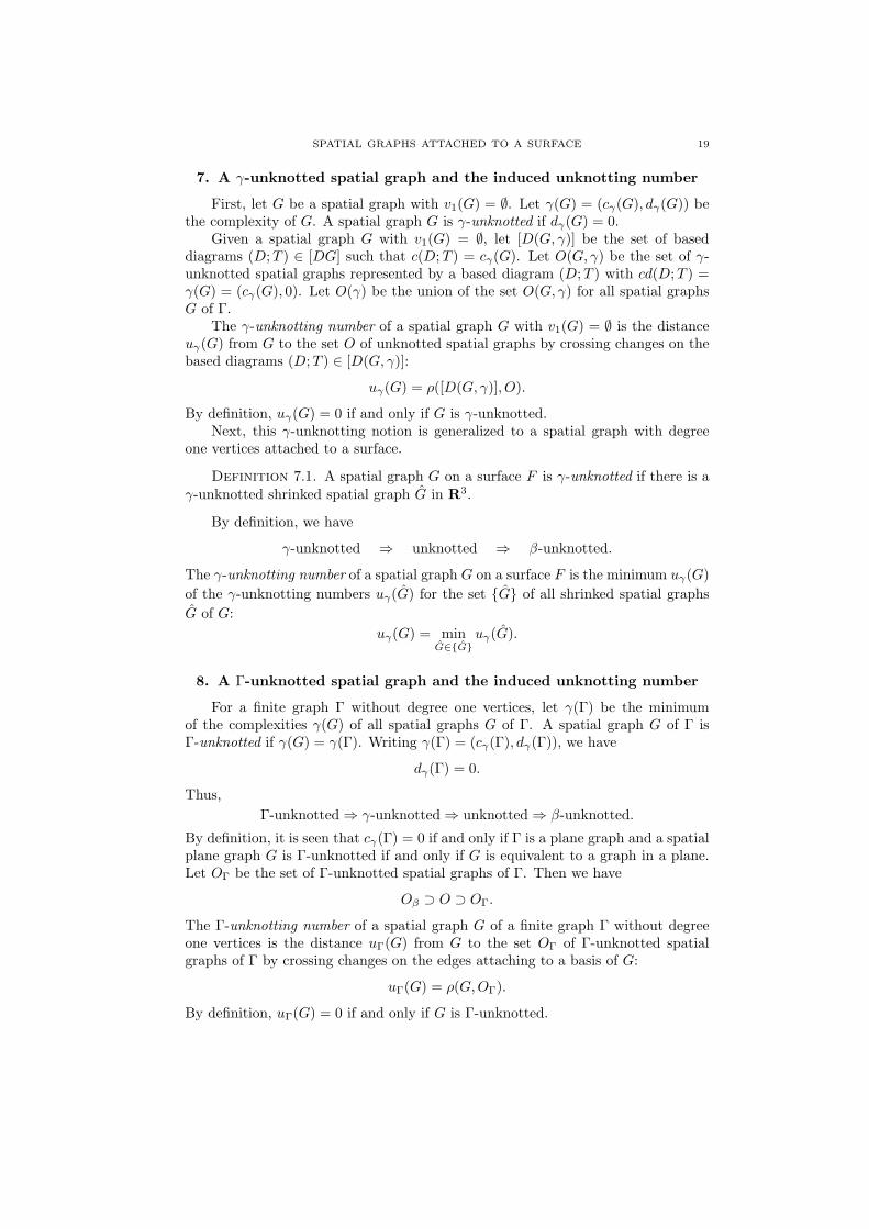
Proof. We note that the exterior E(G∗) is obtained from the exterior E(G)by surgeries of (±1)-framed 2-handles D2 ×D2

k (k = 1, 2, . . . , n) along zero-linkingloops like a loop O in Figure 22. Let

W = E(G)× [0, 1]

n∪k=1

D2 ×D2k

be the compact 4-manifold which is the surgery trace from E(G) to E(G∗) onthe 2-handles D2 × D2

k (k = 1, 2, . . . , n), which is also the surgery trace fromE(G∗) to E(G) on the “dual 2-handles”D2 ×D2

k (k = 1, 2, . . . , n) (see Figure 23).By construction, χ and χ∗ extend to an epimorphism χ+ : H1(W ) → Z. Let

(W ; E(G), E(G∗)) be the infinite cyclic covering triad of the triad (W ;E(G), E(G∗))associated with χ+. Let m(W ;χ+) be the minimal number of Λ-generators of the

Λ-module H1(W ). Because the natural homomorphisms π1(E(G)) → π1(W ) and

π1(E(G∗)) → π1(W ) are onto, so that the natural homomorphisms H1(E(G)) →H1(W ) and H1(E(G∗)) → H1(W ) are onto. Thus, we have　

m(W ;χ+) ≤ m(G,T ;χ) and m(W ;χ+) ≤ m(G∗, T ;χ∗).

By the exact sequence

H2(W , E(G)) → H1(E(G)) → H1(W ) → 0

of the pair (W , E(G)) and the computation H2(W , E(G)) ∼= Λn with a Λ-basisrepresented by the 2-handle cores D2 × 0k (k = 1, 2, . . . , n), we obtain

m(G,T ;χ) ≤ n+m(W ;χ+) ≤ n+m(G∗, T ;χ∗).

Similarly, we have:

m(G∗, T ;χ∗) ≤ n+m(W ;χ+) ≤ n+m(G,T ;χ).

Thus, we have|m(G,T ;χ)−m(G∗, T ;χ∗)| ≤ n.

□

Figure 23. The surgery trace


7. A γ-unknotted spatial graph and the induced unknotting number

First, let G be a spatial graph with v1(G) = ∅. Let γ(G) = (cγ(G), dγ(G)) bethe complexity of G. A spatial graph G is γ-unknotted if dγ(G) = 0.

Given a spatial graph G with v1(G) = ∅, let [D(G, γ)] be the set of baseddiagrams (D;T ) ∈ [DG] such that c(D;T ) = cγ(G). Let O(G, γ) be the set of γ-unknotted spatial graphs represented by a based diagram (D;T ) with cd(D;T ) =γ(G) = (cγ(G), 0). Let O(γ) be the union of the set O(G, γ) for all spatial graphsG of Γ.

The γ-unknotting number of a spatial graph G with v1(G) = ∅ is the distanceuγ(G) from G to the set O of unknotted spatial graphs by crossing changes on thebased diagrams (D;T ) ∈ [D(G, γ)]:

uγ(G) = ρ([D(G, γ)], O).

By definition, uγ(G) = 0 if and only if G is γ-unknotted.Next, this γ-unknotting notion is generalized to a spatial graph with degree

one vertices attached to a surface.

Definition 7.1. A spatial graph G on a surface F is γ-unknotted if there is aγ-unknotted shrinked spatial graph G in R3.

By definition, we have

γ-unknotted ⇒ unknotted ⇒ β-unknotted.

The γ-unknotting number of a spatial graph G on a surface F is the minimum uγ(G)

of the γ-unknotting numbers uγ(G) for the set {G} of all shrinked spatial graphs

G of G:

uγ(G) = minG∈{G}

uγ(G).

8. A Γ-unknotted spatial graph and the induced unknotting number

For a finite graph Γ without degree one vertices, let γ(Γ) be the minimumof the complexities γ(G) of all spatial graphs G of Γ. A spatial graph G of Γ isΓ-unknotted if γ(G) = γ(Γ). Writing γ(Γ) = (cγ(Γ), dγ(Γ)), we have

dγ(Γ) = 0.

Thus,

Γ-unknotted ⇒ γ-unknotted ⇒ unknotted ⇒ β-unknotted.

By definition, it is seen that cγ(Γ) = 0 if and only if Γ is a plane graph and a spatialplane graph G is Γ-unknotted if and only if G is equivalent to a graph in a plane.Let OΓ be the set of Γ-unknotted spatial graphs of Γ. Then we have

Oβ ⊃ O ⊃ OΓ.

The Γ-unknotting number of a spatial graph G of a finite graph Γ without degreeone vertices is the distance uΓ(G) from G to the set OΓ of Γ-unknotted spatialgraphs of Γ by crossing changes on the edges attaching to a basis of G:

uΓ(G) = ρ(G,OΓ).

By definition, uΓ(G) = 0 if and only if G is Γ-unknotted.

20 AKIO KAWAUCHI

The (γ,Γ)-unknotting number uγ,Γ(G) of a spatial graph G of a finite graph Γwithout degree one vertices is the distance from the set [D(G, γ)] to OΓ by crossingchanges on the edges attaching to a basis:

uγ,Γ(G) = ρ([D(G, γ)], OΓ).

By definition, uγ,Γ(G) = 0 if and only if G is (γ,Γ)-unknotted, and

(γ,Γ)-unknotted ⇒ Γ-unknotted

⇒ γ-unknotted ⇒ unknotted ⇒ β-unknotted.

Next, the Γ-unknotting and (γ,Γ)-unknotting notions are generalized to a spa-tial graph with degree one vertices attached to a surface. Let Γ be a finite graphwith degree one vertices.

Definition 8.1. A spatial graph G of Γ on a surface F is Γ-unknotted if thereis a Γ-unknotted shrinked spatial graph G in R3 for the finite shrinked graph Γ ofΓ associated with F .

The Γ-unknotting number of a spatial graph G on a surface F is the minimumuΓ(G) among the Γ-unknotting numbers uΓ(G) for the set {G} of all shrinked

spatial graphs G of the finite shrinked graph Γ of Γ associated with F :

uΓ(G) = minG∈{G}

uΓ(G).

The (γ,Γ)-unknotting number of a spatial graph G on a surface F is the mini-

mum uγ,Γ(G) among the (γ, Γ)-unknotting numbers uγ,Γ(G) for the set {G} of all

shrinked spatial graphs G of the finite shrinked graph Γ of Γ associated with F :

uΓ(G) = minG∈{G}

u(γ,Γ)(G).

Since the introduction of all the unknotting notions is finished, we answer hereQuestion 1.1 in the introduction.

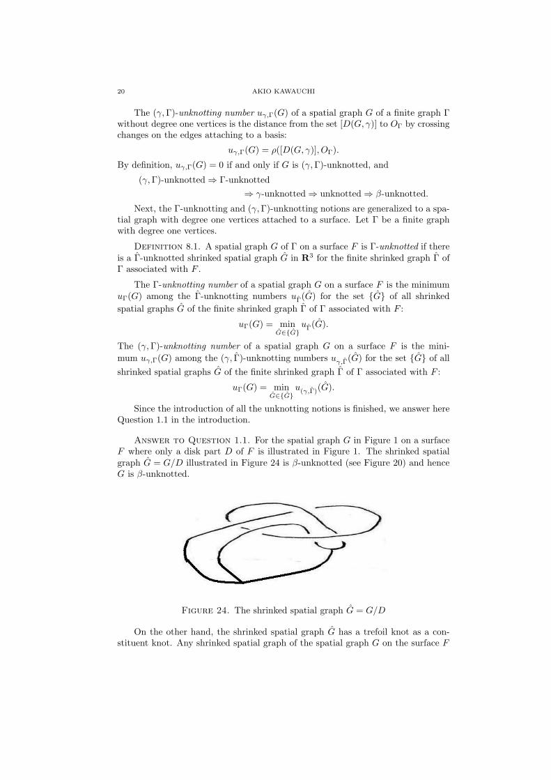
Answer to Question 1.1. For the spatial graph G in Figure 1 on a surfaceF where only a disk part D of F is illustrated in Figure 1. The shrinked spatialgraph G = G/D illustrated in Figure 24 is β-unknotted (see Figure 20) and henceG is β-unknotted.

Figure 24. The shrinked spatial graph G = G/D

On the other hand, the shrinked spatial graph G has a trefoil knot as a con-stituent knot. Any shrinked spatial graph of the spatial graph G on the surface F


is a degree 3 vertex connected sum G(θ) of G and a θ-curve (see Moriuchi [23]),

which has the trefoil knot as a connected direct summand. Hence G(θ) is knotted,so that the spatial graph G on the surface F is (γ,Γ)-knotted, Γ-knotted, γ-knottedand knotted. □

9. The values taken by these unknotting numbers

We show the following two theorems on the values taken by the unknottingnumbers defined in Sections 4-8:

Theorem 9.1. The unknotting numbers

uβ(G), u(G), uγ(G), uΓ(G), uγ,Γ(G)

of any spatial graph G on any surface F satisfy the following inequalities:

uβ(G) ≤ u(G) ≤ {uγ(G), uΓ(G)} ≤ uγ,Γ(G).

Further, these unknotting numbers are distinct for some spatial graphs G on the 2-sphere F = S2. In particular, the large-small relation on uγ(G) and uΓ(G) dependson a choice of spatial graphs G on F = S2.

Theorem 9.2. For any given finite graph Γ, any surface F in R3 and anyinteger n ≥ 1, there are infinitely many spatial graphs G of Γ on F such that

uβ(G) = u(G) = uγ(G) = uΓ(G) = uγ,Γ(G) = n.

We show Theorem 9.1.

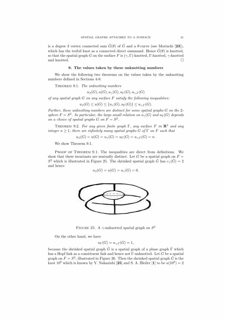
Proof of Theorem 9.1. The inequalities are direct from definitions. Weshow that these invariants are mutually distinct. Let G be a spatial graph on F =S2 which is illustrated in Figure 25. The shrinked spatial graph G has cγ(G) = 2and hence

uβ(G) = u(G) = uγ(G) = 0.

Figure 25. A γ-unknotted spatial graph on S2

On the other hand, we have

uΓ(G) = uγ,Γ(G) = 1,

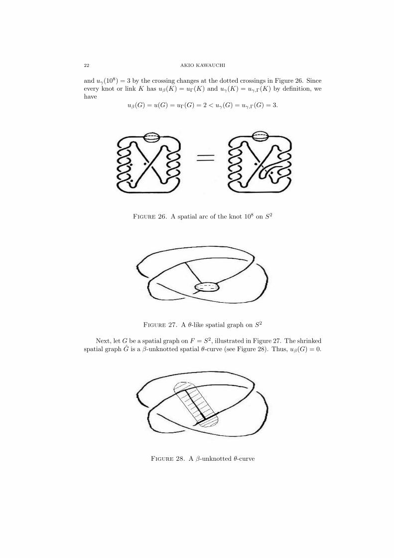
because the shrinked spatial graph G is a spatial graph of a plane graph Γ whichhas a Hopf link as a constituent link and hence not Γ-unknotted. Let G be a spatialgraph on F = S2, illustrated in Figure 26. Then the shrinked spatial graph G is theknot 108 which is known by Y. Nakanishi [25] and S. A. Bleiler [1] to be u(108) = 2

22 AKIO KAWAUCHI

and uγ(108) = 3 by the crossing changes at the dotted crossings in Figure 26. Since

every knot or link K has uβ(K) = uΓ(K) and uγ(K) = uγ,Γ(K) by definition, wehave

uβ(G) = u(G) = uΓ(G) = 2 < uγ(G) = uγ,Γ(G) = 3.

Figure 26. A spatial arc of the knot 108 on S2

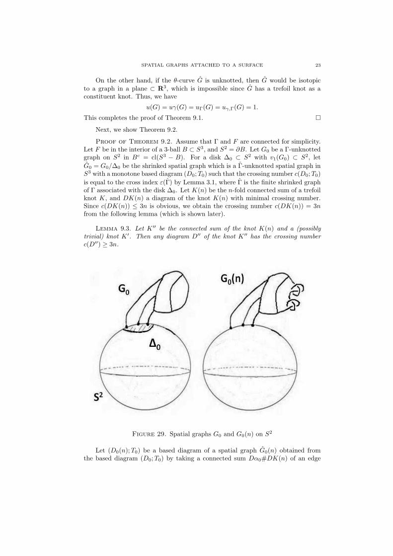
Figure 27. A θ-like spatial graph on S2

Next, let G be a spatial graph on F = S2, illustrated in Figure 27. The shrinkedspatial graph G is a β-unknotted spatial θ-curve (see Figure 28). Thus, uβ(G) = 0.

Figure 28. A β-unknotted θ-curve


On the other hand, if the θ-curve G is unknotted, then G would be isotopicto a graph in a plane ⊂ R3, which is impossible since G has a trefoil knot as aconstituent knot. Thus, we have

u(G) = uγ(G) = uΓ(G) = uγ,Γ(G) = 1.

This completes the proof of Theorem 9.1. □Next, we show Theorem 9.2.

Proof of Theorem 9.2. Assume that Γ and F are connected for simplicity.Let F be in the interior of a 3-ball B ⊂ S3, and S2 = ∂B. Let G0 be a Γ-unknottedgraph on S2 in Bc = cl(S3 − B). For a disk ∆0 ⊂ S2 with v1(G0) ⊂ S2, let

G0 = G0/∆0 be the shrinked spatial graph which is a Γ-unknotted spatial graph inS3 with a monotone based diagram (D0;T0) such that the crossing number c(D0;T0)

is equal to the cross index ε(Γ) by Lemma 3.1, where Γ is the finite shrinked graphof Γ associated with the disk ∆0. Let K(n) be the n-fold connected sum of a trefoilknot K, and DK(n) a diagram of the knot K(n) with minimal crossing number.Since c(DK(n)) ≤ 3n is obvious, we obtain the crossing number c(DK(n)) = 3nfrom the following lemma (which is shown later).

Lemma 9.3. Let K ′′ be the connected sum of the knot K(n) and a (possiblytrivial) knot K ′. Then any diagram D′′ of the knot K ′′ has the crossing numberc(D′′) ≥ 3n.

Figure 29. Spatial graphs G0 and G0(n) on S2

Let (D0(n);T0) be a based diagram of a spatial graph G0(n) obtained fromthe based diagram (D0;T0) by taking a connected sum Dα0#DK(n) of an edge

24 AKIO KAWAUCHI

diagram Dα0 of (D0;T0) and the knot diagram DK(n) so that we have the crossingnumber

c(D0(n);T0) = c(D0;T0) + c(DK(n) = ε(Γ) + 3n

(see Figure 29). Then we show that (D0(n);T0) ∈ [D(G0(n), γ)]. In fact, every

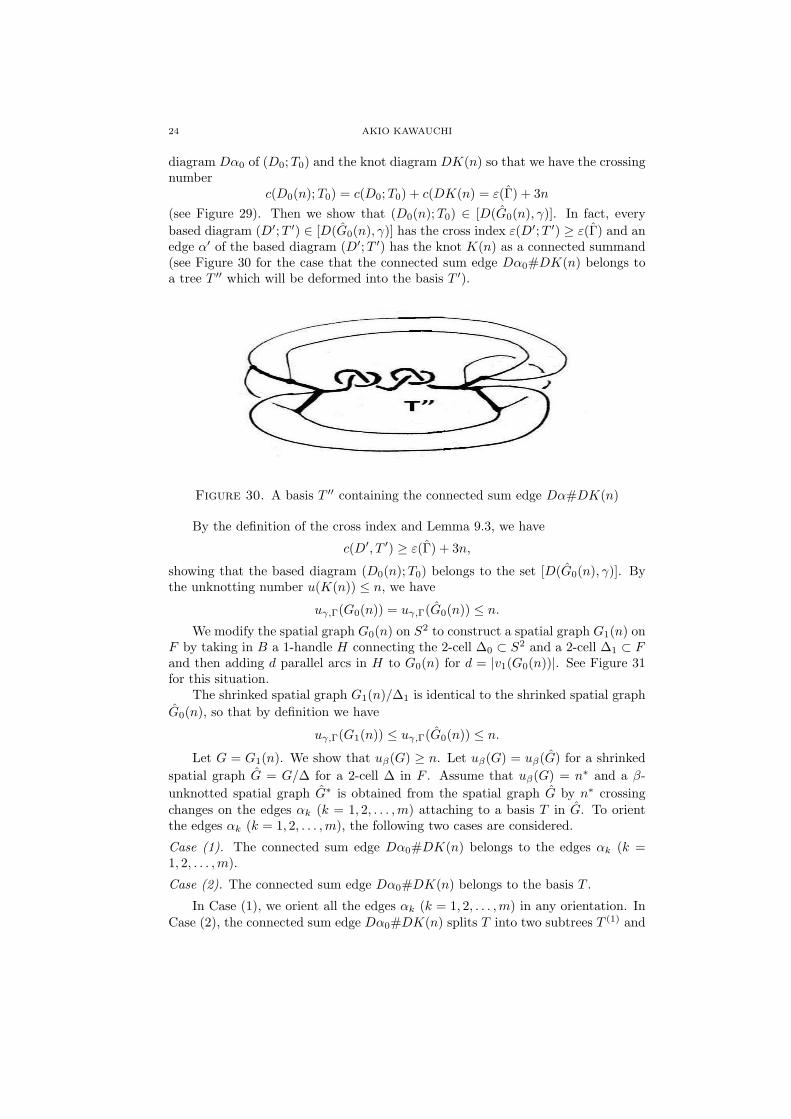
based diagram (D′;T ′) ∈ [D(G0(n), γ)] has the cross index ε(D′;T ′) ≥ ε(Γ) and anedge α′ of the based diagram (D′;T ′) has the knot K(n) as a connected summand(see Figure 30 for the case that the connected sum edge Dα0#DK(n) belongs toa tree T ′′ which will be deformed into the basis T ′).

Figure 30. A basis T ′′ containing the connected sum edge Dα#DK(n)

By the definition of the cross index and Lemma 9.3, we have

c(D′, T ′) ≥ ε(Γ) + 3n,

showing that the based diagram (D0(n);T0) belongs to the set [D(G0(n), γ)]. Bythe unknotting number u(K(n)) ≤ n, we have

uγ,Γ(G0(n)) = uγ,Γ(G0(n)) ≤ n.

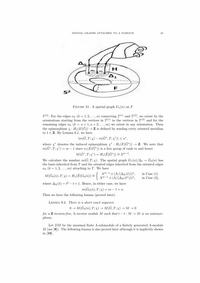
We modify the spatial graph G0(n) on S2 to construct a spatial graph G1(n) onF by taking in B a 1-handle H connecting the 2-cell ∆0 ⊂ S2 and a 2-cell ∆1 ⊂ Fand then adding d parallel arcs in H to G0(n) for d = |v1(G0(n))|. See Figure 31for this situation.

The shrinked spatial graph G1(n)/∆1 is identical to the shrinked spatial graph

G0(n), so that by definition we have

uγ,Γ(G1(n)) ≤ uγ,Γ(G0(n)) ≤ n.

Let G = G1(n). We show that uβ(G) ≥ n. Let uβ(G) = uβ(G) for a shrinked

spatial graph G = G/∆ for a 2-cell ∆ in F . Assume that uβ(G) = n∗ and a β-

unknotted spatial graph G∗ is obtained from the spatial graph G by n∗ crossingchanges on the edges αk (k = 1, 2, . . . ,m) attaching to a basis T in G. To orientthe edges αk (k = 1, 2, . . . ,m), the following two cases are considered.

Case (1). The connected sum edge Dα0#DK(n) belongs to the edges αk (k =1, 2, . . . ,m).

Case (2). The connected sum edge Dα0#DK(n) belongs to the basis T .

In Case (1), we orient all the edges αk (k = 1, 2, . . . ,m) in any orientation. InCase (2), the connected sum edge Dα0#DK(n) splits T into two subtrees T (1) and


Figure 31. A spatial graph G1(n) on F

T (2). For the edges αk (k = 1, 2, . . . , u) connecting T (1) and T (2), we orient by theorientations starting from the vertices in T (1) to the vertices in T (2) and for theremaining edges αk (k = u + 1, u + 2, . . . ,m) we orient in any orientation. Then

the epimorphism χ : H1(E(G)) → Z is defined by sending every oriented meridianto 1 ∈ Z. By Lemma 6.1, we have

|m(G, T ;χ)−m(G∗, T ;χ∗)| ≤ n∗,

where χ∗ denotes the induced epimorphism χ∗ : H1(E(G∗)) → Z. We note that

m(G∗, T ;χ∗) = m− 1 since π1(E(G∗)) is a free group of rank m and hence

M(G∗, T ;χ∗) = H1(E(G∗)) ∼= Λm−1.

We calculate the number m(G, T ;χ). The spatial graph G1(n)/∆1 = G0(n) hasthe basis inherited from T and the oriented edges inherited from the oriented edgesαk (k = 1, 2, . . . ,m) attaching to T . We have

M(G0(n), T ;χ) = H1(E(G0(n)) ∼={

Λm−1 ⊕ (Λ/(∆K(t)))n, in Case (1)Λm−1 ⊕ (Λ/(∆K(tu)))n, in Case (2),

where ∆K(t) = t2 − t+ 1. Hence, in either case, we have

m(G0(n), T ;χ) = m− 1 + n.

Then we have the following lemma (proved later).

Lemma 9.4. There is a short exact sequence

0 → M(G0(n), T ;χ) → M(G, T ;χ) → M → 0

for a Z-torsion-free, Λ-torsion module M such that t− 1 : M → M is an automor-phism.

Let DM be the maximal finite Λ-submodule of a finitely generated Λ-moduleM (see [9]). The following lemma is also proved later although it is implicitly shownin [10].

26 AKIO KAWAUCHI

Lemma 9.5. Let M ′ be a Λ-submodule of a finitely generated Λ-module M . Letb′ and b be the minimal numbers of Λ-generators of M ′ and M , respectively. If themaximal finite Λ-submodule D(M/M ′) of M/M ′ is 0, then we have b′ ≤ b.

By Lemmas 9.4 and 9.5, we have

m(G0(n), T ;χ) ≤ m(G, T ;χ),

because DM = 0, so that

n = (m− 1 + n)− (m− 1)

= m(G0(n), T ;χ)−m(G∗, T ;χ∗)

≤ m(G, T ;χ)−m(G∗, T ;χ∗)

≤ n∗.

Hence uβ(G) ≥ n and

uβ(G) = u(G) = uγ(G) = uΓ(G) = uγ,Γ(G) = n.

This completes the proof of Theorem 9.2 except the proofs of Lemmas 9.3, 9.4 and9.5. □

The proofs of Lemmas 9.3, 9.4 and 9.5 are given as follows.

Proof of Lemma 9.3. It is well-known that the span of the Jones polyno-mial VK′′(t) of the knot K ′′ is smaller than or equal to c(D′′) (see Murasugi [24],Kauffman [7]). Since

VK′′(t) = VK(t)n · VK′(t), VK(t) = t+ t3 − t4

by taking a positive trefoil knot as K, we see that c(D′′) ≥ 3n. □

Proof of Lemma 9.4. The spatial graph G is a degree d vertex connectedsum of the spatial graph G0(n) and a θd-curve Θ relative to the vertex v1 obtained

from v1(G0(n)) and a vertex v2 of Θ (see [23]). In precise, G is the union of

G0(n)′ = cl(G0(n)\B1 ∩ G0(n)) ⊂ Bc

1 and Θ′ = cl(Θ\B2 ∩ Θ) ⊂ Bc2 where Bi is

a 3-ball regular neighborhood of vi in S3 for i = 1, 2. Then the exterior E(G)

is the union of the exteriors E(G0(n)) and E(Θ) with as the intersection part a

compact dth punctured 2-sphere S(d) in the boundaries ∂E(G0(n)) and ∂E(Θ). Let

S(d)c = cl(∂E(Θ)\S(d)). Let E(G0(n)), E(Θ), S(d) and S(d)c be the connected

lifts of E(G0(n)), E(Θ), S(d) and S(d)c to the infinite cyclic covering E(G) of

E(G), respectively. By excision, there is a natural isomorphism

Hd(E(G), E(G0(n)) ∼= Hd(E(Θ), S(d)).

Since H1(E(Θ), S(d)) = H1(E(Θ), S(d)c) = 0, we see from the Wang exact se-

quence that M = H1(E(Θ), S(d)) and M c = H1(E(Θ), S(d)c) are finitely gener-ated Λ-modules such that t−1 : M → M and t−1 : M c → M c are automorphisms,implying that M and M c are Λ-torsion modules whose Z-torision parts τ(M) andτ(M c) are equal to the maximal finite Λ-modules DM and DM c, respectively (see[9]). By the second duality theorem in [9],

τ(M) = DM ∼= Ext1Λ(Mc/TorΛ(M

c); Λ) = 0.


(Note: Though we have also τ(M c) = DM c = 0, we do not use this fact.) Then

the homology exact sequence of the pair (E(G), E(G0(n)) induces a desired exactsequence. □

Proof of Lemma 9.5. For a Λ-epimorphism f : Λb → M , let

B′ = f−1(M ′) ⊂ Λb,

which is a finitely generated Λ-module mapped onto M ′ by f . Since the quotientΛ-module Λb/B′ is isomorphic to M/M ′, which has a Λ-projective dimension ≤ 1since the maximal finite Λ-submodule D(M/M ′) of M/M ′ is 0 (see [9]). Hence

B′ ∼= Λc′ for some nonnegative integer c′, implying that b′ ≤ c′ ≤ b. □

10. Knotting dynamics of a spatial graph with degree one free vertices

In this section, we consider a spatial graph G with degree one vertices v1, v2, . . . ,vd(d ≥ 1) neither of which is not attached to any surface. These degree one verticesare referred to as free vertices. We explain here knotting dynamics of a spatial graphG with degree one free vertices by applying the knotting notions on the spatialgraphs without degree one vertices associated with G. This notion is introduced in[17, 18]. We need to impose a mild restriction on a spatial graph with degree onefree vertices. A spatial graph G with degree one free vertices is normal if G has thefollowing properties (1) and (2) where V = {v1, v2, . . . , vd}:(1) There is a set X = {x1, x2, . . . , vd} of mutually distinct d points in G\V suchthat the line segments |vixi| (i = 1, 2, . . . , d) are mutually disjoint and intersect Gonly in the set V ∪X. (We call the set X a coupling with V .)

(2) There are only finitely many equivalence classes of the spatial graphs (withoutdegree one vertices)

GX = G

d∪i=1

|vixi|

for all couplings X with V .

Every polygonal spatial graph G with degree one free vertices which is notin a plane is normal and if G is normal in a plane ⊂ R3, then the spatial graphGX without degree one vertices is always a Γ-unknotted spatial graph for everycoupling X with V . For every normal spatial graph G with degree one free verticesand every coupling X with V , the unknotting number u(GX) of the spatial graphGX without degree one vertices is defined in Section 4. An analysis on the dynamicsof the invariant u(GX) for every coupling X with V will be useful in studying aknotted structure of the normal spatial graph G with degree one free vertices. Theunknotting number u(G) of a normal spatial graph G with degree one free verticesis defined to be

u(G) = max{u(GX)|X is a coupling withV }.Let nG be the number of distinct equivalence classes on the spatial graphs GX forall couplings X with V , and nG the number of distinct equivalence classes of spatialgraphs GX with u(GX) > 0 for all couplings X with V . The knotting probability ofa normal spatial graph G with degree one free vertices is defined by the fraction

p(G) =nG

nG,

28 AKIO KAWAUCHI

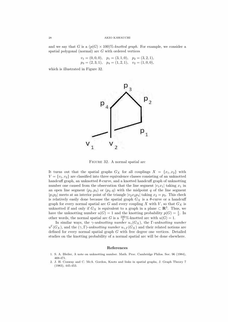
and we say that G is a (p(G) × 100)%-knotted graph. For example, we consider aspatial polygonal (normal) arc G with ordered vertices

v1 = (0, 0, 0), p1 = (3, 1, 0), p2 = (3, 2, 1),p3 = (2, 3, 1), p4 = (1, 2, 1), v2 = (1, 0, 0),

which is illustrated in Figure 32.

Figure 32. A normal spatial arc

It turns out that the spatial graphs GX for all couplings X = {x1, x2} withV = {v1, v2} are classified into three equivalence classes consisting of an unknottedhandcuff graph, an unknotted θ-curve, and a knotted handcuff graph of unknottingnumber one caused from the observation that the line segment |v1x1| taking x1 inan open line segment (p2, p3) or (p2, q) with the midpoint q of the line segment|p1p2| meets at an interior point of the triangle |v2x2p4| taking x2 = p3. This checkis relatively easily done because the spatial graph GX is a θ-curve or a handcuffgraph for every normal spatial arc G and every coupling X with V , so that GX isunknotted if and only if GX is equivalent to a graph in a plane ⊂ R3. Thus, wehave the unknotting number u(G) = 1 and the knotting probability p(G) = 1

3 . In

other words, the normal spatial arc G is a 1003 %-knotted arc with u(G) = 1.

In similar ways, the γ-unknotting number uγ(GX), the Γ-unknotting numberuΓ(GX), and the (γ,Γ)-unknotting number uγ,Γ(GX) and their related notions aredefined for every normal spatial graph G with free degree one vertices. Detailedstudies on the knotting probability of a normal spatial arc will be done elsewhere.

References

1. S. A. Bleiler, A note on unknotting number. Math. Proc. Cambridge Philos. Soc. 96 (1984),469-471.

2. J. H. Conway and C. McA. Gordon, Knots and links in spatial graphs, J. Graph Theory 7(1983), 445-453.


3. T. Endo and T. Otsuki, Notes on spatial representations of graphs, Hokkaido Math. J. 23

(1994) 383-398.4. S. Fujimura, On the ascending number of knots, thesis, Hiroshima University (1988).5. T. S. Fung, Immersions in knot theory, a dissertation, Columbia University (1996).6. S. Kamada, A. Kawauchi and T. Matumoto, Combinatorial moves on ambient isotopic sub-

manifolds in a manifold, J. Math. Soc. Japan 53 (2001),321-331.7. L. H. Kauffman, State models and the Jones polynomial, Topology 26 (1987), 395407.8. L. H. Kauffman, Invariants of graphs in three space, Trans. Amer. Math. Soc. 311 (1989),

697-710.

9. A. Kawauchi, Three dualities on the integral homology of infinite cyclic coverings of manifolds,Osaka J. Math. 23 (1986), 633-651.

10. A. Kawauchi, On the integral homology of infinite cyclic coverings of links, Kobe J. Math. 4(1987),31-41.

11. A. Kawauchi, An imitation theory of manifolds, Osaka J. Math. 26 (1989), 447-464.12. A. Kawauchi, Almost identical imitations of (3,1)-dimensional manifold pairs, Osaka J. Math.

26 (1989), 743-758.13. A. Kawauchi, Almost identical link imitations and the skein polynomial, Knots 90, Walter de

Gruyter (1992), 465-476.14. A. Kawauchi, Distance between links by zero-linking twists, Kobe J. Math. 13(1996), 183-190.15. A. Kawauchi, A survey of knot theory, Birkhauser (1996).

16. A. Kawauchi, Lectures on knot theory (in Japanese), Kyoritu Shuppan (2007).17. A. Kawauchi, On a complexity of a spatial graph, in: Knots and soft-matter physics, Topology

of polymers and related topics in physics, mathematics and biology, Bussei Kenkyu 92-1 (2009-4), 16-19.

18. A. Kawauchi, On transforming a spatial graph into a plane graph, in: Statistical Physics andTopology of Polymers with Ramifications to Structure and Function of DNA and Proteins,Progress of Theoretical Physics Supplement, No. 191 (2011), 235-244.

19. A. Kawauchi and K. Yoshida, Topology of prion proteins, Journal of Mathematics and System

Science 2 (2012), 237-248.20. S. Kinoshita, On θn-curves in R3 and their constituent knots, in:Topology and Computer

Science , Kinokuniya Co. Ltd. (1987), 211-216.21. S. Kinoshita, On spatial bipartite Km,n’s and their constituent K2,n’s, Kobe J. Math. 8

(1991), 41-46.22. W. B. R. Lickorish and K. C. Millett, A polynomial invariant of oriented links, Topology 26

(1987), 107-141.23. H. Moriuchi, Enumeration of algebraic tangles with applications to theta-curves and handcuff

graphs, Kyungpook Math. J. 48 (2008), 337-357.24. K. Murasugi, Jones polynomials and classical conjectures in knot theory, Topology 26 (1987),

187194.

25. Y. Nakanishi, Unknotting numbers and knot diagrams with the minimum crossings. Math.Sem. Notes Kobe Univ. 11 (1983), no. 2, 257-258.

26. M. Okuda, A determination of the ascending number of some knots, thesis, Hiroshima Uni-versity, 1998.

27. M. Ozawa, Ascending number of knots and links. J. Knot Theory Ramifications 19 (2010),15-25.

28. M. Ozawa and Y. Tsutsumi, Primitive spatial graphs and graph minors. Rev. Mat. Complut.20 (2007), 391-406.

29. A. Shimizu, The warping degree of a knot diagram, J. Knot Theory Ramifications 19 (2010),849-857.

30. A. Shimizu, The warping degree of a link diagram, Osaka J. Math. 48 (2011), 209-231.31. R. Shinjo, Bounding disks to a spatial graph. J. Knot Theory Ramifications 15 (2006), 1225-

1230.

Osaka City University Advanced Mathematical Institute, Sugimoto, Sumiyoshi-ku,Osaka 558-8585, Japan

E-mail address: [email protected]

Documents

Knot Theory For Spatial Graphs Attached To A Surfacekawauchi/KnotTheoryforSpatial...Knot Theory For Spatial Graphs Attached To A Surface Akio Kawauchi Abstract. Beside a survey on