Joint Model I

Kinetics and Muscle Modeling of a Single Degree of Freedom Joint Part I: Mechanics

Rick Wells

July 28, 2003

I. Introduction This will be a two-part tech brief on dynamical modeling of the skeletomuscle system of a single jointed limb comprised of a fixed-position bone, a movable bone, and two muscles arranged as an agonist-antagonist pair. Part I will deal with modeling the mechanics of the system. Part II will deal with the modeling of the sensory neurons. My intent in this tech brief is to provide the mathematical foundation for more advanced systems comprised of multiple joints and multiple degrees of freedom. At the outset it seems necessary to make a brief comment on why I have chosen this particular model for our bipedal locomotion work. In particular, why go into such detail in modeling the behavioral characteristics of muscles when it is obvious that any mechanical system we might eventually build will not be made out of biological material. As I see it, there are two motivating factors for this approach. In the first place, the biologically-based model presents us with a number of nonlinearities in the dynamical equations describing the system. To my way of thinking, the application of neural networks to the control of linear systems is a rather pointless endeavor because the linear system can be controlled less expensively, and with a much greater mathematical foundation, by the well-established methods of modern control theory. On the other hand, the control of nonlinear systems is much less well understood by standard theory and usually requires nonlinear elements in its controller. One example of this is the application of variable-structure switching control systems. Another is the use of fuzzy or neurofuzzy control methods. I have already mentioned, in a previous tech brief, that the spinal sensorimotor control system appears to implement a sophisticated form of VSSC. In the second place, developing methods capable of dealing with the nasty and sometimes harsh realities of the nonlinear skeletomuscle system model presented here seems to me a fruitful path for later dealing with some sometimes nasty nonlinear factors in man-made electro-mechanical systems. For example, a mobile robot must be made lightweight if it is to operate for any appreciable length of time using battery power. Achieving light weight in a robotic platform implies several things. It implies the use of low-density materials in the construction of the chassis, and although low-density materials with high tensile strength do exist, inexpensive low-density materials tend to depart rather noticeably from “rigid body” behavior. For example, it is nice if the teeth of a plastic gear are rigid, but unless a very hard plastic is used they won’t be. Stepper motors are widely available, but lightweight stepper motors are small, have highly variable speed-torque characteristics, and exhibit a number of nasty nonideal departures from the rather simplified motor models presented in a junior-level electric motor course. The use of cables (strings, really) to actuate limb movement is a lightweight alternative to installing rotary actuator motors at joints, but when cables are introduced as the actuator means we take a big step toward the biological method since muscles and tendons are really nothing more than meat cables. Cables stretch, go slack, and otherwise exhibit a number of similarities to the type of non-linearities the model presented here discusses.

1

Joint Model I

�

�

�

L4

L1L3

mg

l1l2 L2

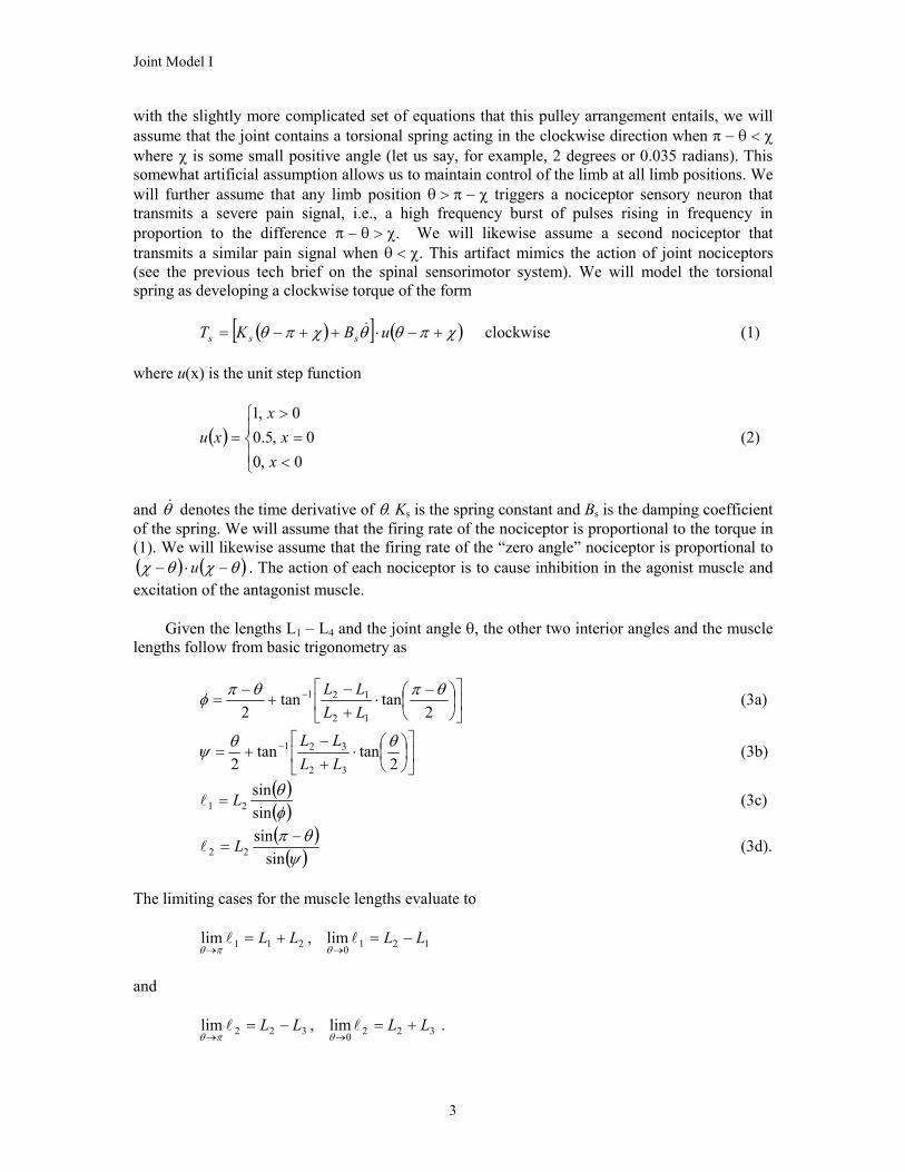
Figure 1: Simplified single-joint limb model. The system has two idealized bones, each modeled as a

rigid body, and two muscles, l1 and l2, modeled as contractible cables. � is the joint angle, taken as positive in the counterclockwise direction. ����� corresponds to the limb handing straight down. m is the mass of

the movable limb, in kilograms, and g is the acceleration due to gravity (9.807 meters per second per second). The weight of the limb is mg and acts at the center of gravity of the limb as shown in the figure.

The limb is modeled, rather ideally, as a homogeneous cylinder of radius r and length L1 + L3 + L4.

Taken together, these two considerations justify, in my mind at least, targeting the bio-mimetic model presented here. Put another way, if we can develop design methods and pulse coded neural networks to control the system presented here, it seems to me very likely that we will be able to do the same for the far-less-sophisticated types of systems man might construct. That, at least, is the justification in my mind for the model presented here.

II. Kinematics and Mechanics of the Movable Limb The model of the limb mechanical system is illustrated in figure 1. The movable limb is approximated as a homogeneous cylinder of radius r, mass m, and length as shown in the figure. It is connected to the fixed bone at a pivot, assumed to be free of friction (another idealization). This figure is a departure from a real skeletomuscle system in two important ways. First, in a real bone-muscle system there would not be the protrusion L3 at the back side of the limb. Instead, muscle l2 would go around a pulley at the joint and attach to the movable bone on the underside. By representing the system as shown in figure 1, I have merely constructed a representation that gives an equivalent mechanical leverage to the movable bone. In the second place, the system shown above suffers loss of muscle control at ����� because at this position the force from either muscle passes directly through the pivot point and center of mass (and therefore can develop no torque). In a real skeletomuscle system, both muscles would wrap around a pulley at the joint and attach to the muscle at some angle that still permits the development of a torque. Rather than deal

2

Joint Model I

with the slightly more complicated set of equations that this pulley arrangement entails, we will assume that the joint contains a torsional spring acting in the clockwise direction when ��������� where � is some small positive angle (let us say, for example, 2 degrees or 0.035 radians). This somewhat artificial assumption allows us to maintain control of the limb at all limb positions. We will further assume that any limb position ��������� triggers a nociceptor sensory neuron that transmits a severe pain signal, i.e., a high frequency burst of pulses rising in frequency in proportion to the difference ���������. We will likewise assume a second nociceptor that transmits a similar pain signal when �����. This artifact mimics the action of joint nociceptors (see the previous tech brief on the spinal sensorimotor system). We will model the torsional spring as developing a clockwise torque of the form � �� � � �������� ������� uBK sss

�T clockwise (1) where u(x) is the unit step function

u (2) � ���

��

�

�

�

�

�

0,00,5.0

0,1

xx

xx

and � denotes the time derivative of �. K�

s is the spring constant and Bs is the damping coefficient of the spring. We will assume that the firing rate of the nociceptor is proportional to the torque in (1). We will likewise assume that the firing rate of the “zero angle” nociceptor is proportional to � � � ���� ��u�� . The action of each nociceptor is to cause inhibition in the agonist muscle and excitation of the antagonist muscle. Given the lengths L1 – L4 and the joint angle �, the other two interior angles and the muscle lengths follow from basic trigonometry as

��

���

���

�

� �

�

�

� �

2tantan

2 12

121 ����

LLLL

� (3a)

��

���

���

�

�

�

��� �

2tantan

2 32

321 ��

LLLL

� (3b)

� �� ���

sinsin

21 L�� (3c)

� �� ��

��

sinsin

22�

� L� (3d).

The limiting cases for the muscle lengths evaluate to 1210211 lim,lim LLLL ���

��

�����

and . 3220322 lim,lim LLLL ���

��

�����

3

Joint Model I

If the tension in muscle 1 produces a force F1 and that of muscle 2 produces force F2 , then the torque produced on the limb by each muscle is given by � ��sin111 ��� FLT clockwise (4a) � ��sin232 ��� FLT counterclockwise (4b). Modeling the limb as a homogeneous cylinder of radius r, the center of mass of the limb is located at

2

341 LLLLcom

��

�

with respect to the axis running down the center of the cylinder and taking the pivot point as the origin of the coordinate system. The torque produced by the weight of the limb is therefore

� ��sin2

341��

��

� mgLLL

wT clockwise (4c).

The net torque acting on the limb, including the contribution by the torsional joint spring (1), is then T counterclockwise (5). swL TTTT ���� 12

In order to find the dynamical equation of motion for the limb we must have the moment of inertia of the limb referenced to the pivot point. For a homogeneous cylinder, the moment of inertia referenced to the center of mass is given by

� �� �2431

2312

LLLrmI com ����� .

To translate the moment of inertia to the pivot point we apply the parallel axis theorem . � �2xmII comj ���

In this case, the displacement �x is equal to the distance of the center of mass from the pivot point. Therefore, after a minor bit of algebra, the moment of inertia about the joint is given as

� � � �

���

�

���

��

����

43

2314

24

231 rLLLLLL

mI j (6).

We next apply Newton’s law for rotational systems and obtain the differential equation describing the motion of the limb as

Lj

TI

��

1��� (7).

4

Joint Model I

For numerical solution of the model equations it is convenient to express (7) in state variable format. We will define � and two state variables, s�� ��� 0 1 and s2 as (8a) ���1s and (8b). �� �� ���2s Applying these to (7) yields the coupled system of equations

� �12

211 sTI

s

ss

Lj��

�

�

�

(9)

where we have explicitly denoted that TL is a function of s1 in (9). The dynamical equation (9) is a coupled set of nonlinear differential equations for which there exists no general closed form solution (so far as I know). Thus we will require a numerical solution. Note also that (9) is a function of muscle forces F1 and F2 , which we must obtain from the model equations for the set of extrafusal muscle fibers making up muscles 1 and 2. Consequently, (9) is also coupled to the muscle model equations presented in section IV.

III. The Hill Model and the Muscle Element Laws Were it possible to write a complete set of equations describing a muscle, which no one has yet accomplished, it is certain that this set of equations would consist of coupled partial differential equations. This is because the muscle is a distributed electro-mechanical-chemical system, and all distributed systems are described by partial differential equations. Equations such as these, even when they are linear, are notoriously difficult to solve because it proves difficult to adequately describe their boundary conditions (which in partial differential equations play the same role that initial conditions play in ordinary differential equations). No one has ever seriously proposed to approach muscle system modeling in this way. What is done instead is that the system is approximated by a set of lumped elements, in much the same way that electric circuit elements are lumped element approximations of Maxwell’s equations. In 1949 A.V. Hill proposed such a lumped-parameter model for the muscle.1 Hill’s model is still in use today, and it remains the most popular form of lumped-element model for the muscle. In point of fact, there are actually two canonical forms of Hill’s model, but these forms are mathematically equivalent under a suitable change of variables.2 The canonical form we employ here is the easier one to apply to a muscle when it is regarded as composed of multiple motor units acting in parallel with one another. Figure 2 illustrates the Hill model. Although this model is typically applied to the whole muscle, for our purposes we will regard the area shown in the yellow background as representing

1 A.V. Hill, “The abrupt transition from rest to activity in muscle”, Proc. Roy. Soc. London B, vol. 136, issue 884 (Oct. 19, 1949), pp. 399-420. 2 T.A. McMahon, Muscles, Reflexes, and Locomotion, Princeton, NJ: Princeton University Press, 1984, pp. 23-25.

5

Joint Model I

TSEC

TC

TBC

B

PEC

SEC

T

TPEC

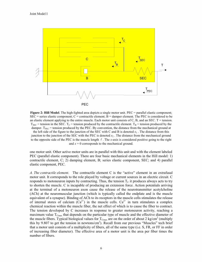
Figure 2: Hill Model. The high-lighted area depicts a single motor unit. PEC = parallel elastic component; SEC = series elastic component; C = contractile element; B = damper element. The PEC is considered to be an elastic element applying to the entire muscle. Each motor unit consists of C, B, and an SEC. T = tension. TSEC = tension in the SEC. TC = tension produced by the contractile element. TB = tension produced by the damper. TPEC = tension produced by the PEC. By convention, the distance from the mechanical ground at

the left side of the figure to the junction of the SEC with C and B is denoted x1 . The distance from this junction to the junction of the SEC with the PEC is denoted x2 . The distance from the mechanical ground to the opposite side of the PEC is the muscle length . The x-axis is considered positive going to the right

and x = 0 corresponds to the mechanical ground. �

one motor unit. Other active motor units are in parallel with this unit and with the element labeled PEC (parallel elastic component). There are four basic mechanical elements in the Hill model: 1) contractile element, C; 2) damping element, B; series elastic component, SEC; and 4) parallel elastic component, PEC. A. The contractile element. The contractile element C is the “active” element in an extrafusal motor unit. It corresponds to the role played by voltage or current sources in an electric circuit. C responds to motoneuron inputs by contracting. Thus, the tension TC it produces always acts to try to shorten the muscle. C is incapable of producing an extension force. Action potentials arriving at the terminal of a motoneuron axon cause the release of the neurotransmitter acetylcholine (ACh) at the neuromuscular junction (which is typically called the endplate and is the muscle equivalent of a synapse). Binding of ACh to its receptors in the muscle cells stimulates the release of internal stores of calcium (Ca2+) in the muscle cells. Ca2+ in turn stimulates a complex chemical reaction within the muscle fiber, the net effect of which is to cause the fiber to contract. The tension developed by C increases in response to greater motoneuron activity, reaching a maximum value TCmax that depends on the particular type of muscle and the effective diameter of the muscle fibers. Typical biological values for TCmax are on the order of about 2 kg/cm2 (multiply this by 9.807 to get the tension in newtons/cm2). Recall from our previous “Muscles” tech brief that a motor unit consists of a multiplicity of fibers, all of the same type (i.e. S, FR, or FF in order of increasing fiber diameter). The effective area of a motor unit is the area per fiber times the number of fibers.

6

Joint Model I

The tension that can be produced for a given level of motoneuron excitation is a function of the ratio of fiber length to its “resting length” . If Q0� C is the tension that would be produced when the contractile unit length is x1 = (see the caption under figure 2), then the tension produced at length x

0�

1 = is given by �

� �01 �xAQCC ��T , T (10a) maxCC T�

where the function A is the tension vs. fiber length characteristic depicted in figure 4 of the “Muscles” tech brief. A reasonable approximation for A within biological limits imposed on the range of muscle lengths possible is given by

� �

� �

� �

� ����

�

���

�

�

����

��

�

�

0101

010

01001

0101

01

05.1,50.27

1005.195.0,1

95.08.0,75.31

34

8.0,40.24

��

��

���

��

�

xx

x

xx

xx

xA (10b).

The function A is always non-negative; separation of the muscle from the bone occurs at values for x1 within the positive-valued range of A given in (10b). The complex dynamics of contraction can be approximated as a leaky integrator. The dynamical equation of the contractile element can therefore be approximated by a single state variable obeying the equation

� �tpC

QCC ����

��

01�Q (11)

where � is the leaky integrator time constant and p(t) is the action potential pulse train. Referring to figure 2 of the “Muscles” tech brief, the time constant for a fast fiber (FR or FF) is on the order of about 10 msec, while for slow S-type fibers the time constant is about 3 to 3.5 times longer. The force constant C0 = TCmax for the motor unit. As noted in the “Muscles” tech brief, FR fibers develop about 4 times more maximum tension than S fibers, and FF-type fibers develop about 2 times more maximum tension than FR-type fibers. There is one additional complication to consider in modeling the contractile element. Under sustained high-frequency bombardment by motoneuron action potentials, a motor unit exhibits desensitization, which is a loss of responsiveness by the muscle fibers to continued AP stimulation. We will postpone discussion of this factor to a later point in this tech brief. For now, it is sufficient to say that desensitization can be modeled as a reduction in C0 due to excess stimulation. This effect is important, in my opinion, because it affects the motoneuron recruitment characteristics that our evolved spinal cord neural networks must employ. B. The Elastic Elements. A muscle when passively stretched exhibits an elastic restoring force that tends to return the muscle to its original length. In part this force is due to stretching the connective tissue that surrounds the muscle fibers. In part it may be due to stretching the tendons which terminate muscle tissue and attach it to the bone. There is reason to believe that the muscle fibers themselves are at least partly elastic. It is this elastic restoring force that is represented by

7

Joint Model I

the elastic elements (springs) in the Hill model. It is not completely correct to assign these elements to any one particular physical source, but for our purposes we may regard the PEC as being mostly due to the connective tissues and the SEC as being primarily dominated by tendon fibers terminating specific motor units. Muscle and tendon fiber stiffness follows a remarkably simple empirical stress-strain relationship. Stress is defined as force per unit cross sectional area of a fiber. Strain is defined as the deformation in length due to an applied stress. The empirical relationship is given by

� ����

����

dd

� (12)

where � is the stress, 0���� is the ratio of length to resting length (sometimes called the slack length), and � and � are empirical constants. Ballpark values for these constants are � = 12 (a dimensionless quantity) and � = 8.3 grams/cm2 (when the stress is expressed in gram-force units). This gives the stress in (12) units of grams/cm2, which can be converted to newtons/cm2 by multiplying it by 9.807�10-3. Evaluating (12) gives us � (13). �� ��

��� e where � is the integrating factor (in units of grams/cm2). We can apply (13) to the PEC by assuming that at the resting length (or slack point) where � = 1 the stress is zero. This gives us � ���� ��� exp . The total force is stress multiplied by the cross sectional area so that the elastic tension produced by the PEC is � �� � � �0

1 1 �� ������� ueAPEC

���T (14) where A is the cross sectional area in cm2. Because muscle density is about 1.0 grams/cm3, the effective cross sectional area of the whole muscle can be estimated from

cminlength

gramsinweightA � .

By defining �� we can re-express (14) in the standard form 0��� �

� �0��� ����� uK PECPECT (15a) where

� �10 ���

��� ��

�

�� eAK PEC (15b)

with

000

lim PECPEC KAK ��

�� ��

�� (15c).

8

Joint Model I

Applying (15c) to (15b) and substituting into (15a) gives us the element law for the PEC as

� 001

��� ������

���

��

ueK PECPEC��

��

�T (16)

where 0������ . The element law for the SEC is similar but does have a slightly different form. This is due to an ambiguity in defining what exactly constitutes the length x2 of the SEC in figure 2. The ambiguity arises because it is not clear what exactly is the physical correspondent to the SEC. It will be mathematically convenient for us to think about the SEC as representing strain in the tendon fibers to which the motor unit attaches, and therefore to regard x2 as representing the length by which the tendon is stretched beyond its resting length. We take x2 = 0 as the relaxed state of the tendon, and therefore x2 < 0 indicates that the tendon is slack. This convention requires us to represent the total muscle length as � (17) � 221 xuxx ��� � where x1 is the length of the contractile element. Under this convention the constant � in (12) is no longer a dimensionless quantity, but rather has units of "per cm". We denote this by �s and write the element law for the SEC in standard form as

� � � � � 22222

0 12 xuxKxuxex

KSEC

x

s

SECSEC

s�������

�

�

�T (18a)

where (18b) sSECK �� ��0

and � is a dimensionless tension constant. Since both terms in (18b) are empirical values, it is probably simplest to simply regard KSEC0 as simply some empirical constant in its own right. (18b) merely ties KSEC0 to the stress-strain law. KPEC and KSEC are known as the stiffnesses of the two elastic elements. We should note that according to equations (15b) and (18a) both these factors are functions of lengths, and therefore the PEC and SEC are nonlinear springs. Because we are associating the SEC with tendon fibers, and tendon fibers are generally more "stiff" than the connective muscle tissue, we can generally assume that KSEC0 > KPEC0. C. The Damper Element. It is an empirical fact that muscle tension during contraction and the speed of the contraction are coupled to each other. Hill found that the relation between them follows a characteristic hyperbolic equation, now known as Hill’s equation. For and total contractile muscle tension T

01 �x�AB = TC + TB (see figure 2), Hill’s equation is

� �� � � � baTxbaT CAB ����� 1� (19)

9

Joint Model I

where a and b are empirically determined constants. Hill’s equation fits the experimental data for ; for muscle stretch ( ) the muscle departs from the behavior predicted by the

equation. We will discuss the modeling of the stretch case in a little while. Substituting T01 �x� 01 �x�

AB = TC + TB into (19) and solving in terms of TB gives us

111

xBxxbaTC

B ���

���

�

�

�T (20)

where B is the damping coefficient. Note that B is a function of both velocity and the tension produced by the contractile element. Although Hill’s equation is deduced only for the whole-muscle case, we will make the assumption that it applies to individual motor units. Ballpark values for a and b (derived from Hill’s studies of toad legs1) are: grams (gram-force) and

(0.2 � muscle length) per second, where muscle length is taken as � in cm. 4�a0�b

There is a maximum speed at which active shortening of the muscle can occur. Solving (19) for the total tension we get

� �

axb

aTb CAB �

�

��

�

1�T .

Since TAB can never be negative (because active muscle force can only contract, it cannot extend), we find the maximum speed of contraction when TAB = 0. Letting contraction speed be defined as

, we get 1xv ���

a

bTv C

�max (21).

It is convenient to define the dimensionless factor

vb

Ta

C��k (22).

At the maximum tension that can be developed by the contractile element, k typically lies in the range . Biological values for per unit area of muscle are on the order of about 2.0 kg/cm

25.015.0 min �� k maxCT2, as noted earlier. At k = 0.25 and T = 2 kg./cmmaxC

2, (22) implies an effective total fiber area of about 8�105 �m2, and the anatomical range of muscle fiber diameters runs from 10 �m to 100 �m per fiber3. The number of fibers depends on the distribution of S-, FR-, and FF-type muscle fibers in the muscle, and we should recall that each motor unit is made up of only one type of muscle fiber. We can use this to develop numerical values for individual motor units as follows.4 Using the whole-muscle range for kmin as given above, the effective area of the muscle is 3 A. Vander, J. Sherman, and D. Luciano, Human Physiology, 7th ed., Boston, MA: McGraw-Hill, 1998, pg. 288. 4 Bear in mind that Hill’s model was developed from whole-muscle experiments. Therefore, parameters such as k as measured by Hill and others reflect whole-muscle characteristics, which we must subdivide to find the appropriate numbers for individual motor units.

10

Joint Model I

2

min

52

min

3

min

1021022000

mk

cmkk

aAeff ��

�

�

�

�

�

�

(23a).

The typical distribution of S-, FR-, and FF-type fibers in a muscle has been characterized by Henneman.5 Letting NS , NFR , and NFF denote the number of S-, FR-, and FF-type fibers, respectively, in the whole muscle, then from Henneman’s distribution I calculate the approximate formula for Aeff based on average fiber diameters5 as (23b). FFFRSeff NNNA ������ 69401963227 where Aeff

is expressed in �m2. These fibers are distributed over the various motor units, subject to the constraint placed upon their total number by (23b). Average fiber diameters for each type of fiber are approximately dS = 17 �m, dFR = 50 �m, dFF = 94 �m and so if a motor unit has nMU fibers (all of the same type with diameter d), then the effective area of the motor unit in �m2 is given by

22

4mdnA MUMU �

� �

��

and the kmin for that motor unit is

2

5

min108

dnk

MU ��

�

�

�

(24a).

The maximum tension in grams that can be developed by that motor unit’s contractile element is then

minmin

0max4

kkaCC ���T grams (24b)

where C0 is the force constant in (10a).

For example, a motor unit consisting of 100 S-type fibers would have a kmin of 8.81 and a C0 of 0.454 grams (86.4�10-3 newtons). Its maximum contraction velocity would be

023.081.82.0

minmax ���

kbv muscle length/sec (= 0.43 cm/sec for = 20 cm). 0�

In comparison, a motor unit with 100 FF-type fibers would have kmin = 0.288, C0 = 13.9 grams, and vmax = 0.694 muscle lengths/sec (= 13.9 cm/sec for a 20 cm muscle).

5 V.B. Brooks, The Neural Basis of Motor Control, NY: Oxford University Press, 1986, pp. 58-60.

11

Joint Model I

In order to be consistent with the maximum tensions illustrated in Figure 2 of the “Muscles” tech brief, the average FF-type motor unit compares to the average S-type motor unit as (25a) � � �SMUFFMU nn �� 26.0 �

�

and the average FR-type motor unit compares to the average S-type motor unit as (25b) � � � �SMUFRMU nn �� 46.0 from which we get n (25c). � � �FRMUFFMU n�� 565.0 These relations give us relative C0 ratios that are self-consistent with measured data. Bear in mind that NS in (23b) is nMU(S) times the number of S-type motor units, and similarly for NFR and NFF. In order to avoid notational confusion later on, let us agree to denote the whole-muscle kmin with the special symbol kw (0.15 < kw < 0.25). Given a kw describing the whole muscle, let us denote the number of motor units in the muscle as GS , GFR , and GFF for the S-, FR-, and FF-type motor units, respectively. From kw we calculate the muscles effective area from (23a). The (23b) can be expressed in terms of the “mix” of motor units and nMU(S) as

� � �SMUFFFRSw

nGGGk

�������

� 1804903227102 5

�

(26).

This constraint equation puts restrictions on the number of different motor units that must be included in the overall model. For example, if we were to simply pick 5 S-type, 2 FR-type and 1 FF-type motor units as comprising a muscle, then with kw = 0.25 equation (26) tells us nMU(S) must be 169 (rounding up to an integer number of fibers). Equations (25) then specify the number of FF- and FR-type fibers per motor unit as 44 and 78, respectively (again rounding to an integer number of fibers). From this and the average fiber diameters given earlier we find kmin and C0 for each motor unit using equations (24). For the example numbers just given, this would be S-type: kmin = 5.21, C0 = 0.767 grams FR-type: kmin = 1.31, C0 = 3.053 grams FF-type: kmin = 0.655. C0 = 6.11 grams for each individual motor unit. The maximum total force the muscle could exert with all motor units active and at their maximum tensions would then be 16 grams (0.157 newtons = 0.035 lbs.), which is consistent with the choice of kw and equation (22).6

6 You may find this maximum force value to be surprisingly small. It is a consequence of our using the “toad value” of a = 4 grams in this derivation. Altering the number of motor units in (26) does not change the maximum force since this is a/kw . Large animals would have either a larger value of a (which affects equation (23a) and our other numbers) or else each “muscle” would actually be made up of parallel combinations of large numbers of “sub-muscles”, giving a greater Aeff for “the muscle”. Judging from anatomical sketches I’ve seen, both strategies seem to be employed together in real animals. Since such “parallel sub-muscles” would be close synergists, for our purposes it is probably sufficient to calculate the “per sub-muscle tension” using the equations given here and apply a “whole muscle force multiplier”.

12

Joint Model I

Hill’s equation has thus allowed us to specify a number of muscle properties. Now, recall that the total tension for a motor unit is determined from (10a) and k is a function of this tension, as per (22). In general, as TC is reduced, k increases and vmax decreases. All this is for active muscle contraction. When the muscle is stretched, the damping properties no longer follow Hill’s equation. There is a slope change in TAB vs. at = 0 and T1x� 1x� AB reaches a saturation value � � 0,1 1max ���� xTm CAB �T (27) where 0.2 < m � 0.8, with 0.8 being a fairly typical value for m. The increase in TAB is due to the damper opposing the stretching of the muscle. From experimental curves the saturation of muscle tension is reached at velocity7

� � maxmax1 1.01.0 vaTb

x C��

��� (28).

Also judging from reported data, we do not appear to introduce very much error if we ignore the aforementioned slope change and simply employ Hill’s equation up to the saturation point. To enforce continuity with Hill’s equation at the maximum stretch velocity we require

� �

� �max1max1

xxb

aTmT C

CB �

��

�

�

��T .

With a minor amount of algebraic manipulation, this gives us

� �� �max11,

1.011.0 xxT

kk

CB �� ��

�

���T .

Combining this with our previous results, we obtain the complete model of the damping

element as

� �

���

�

���

�

�

���

���

�

������

�

vxT

vxTk

k

vxvxxbaT

C

C

C

B

1

1

111

,

1.0,1.0

11.0

1.0,

�

�

���

T (29).

The first term in (29) is in the form of a nonlinear viscous damper with damping coefficient B depending on velocity and contractile force TC . We will call this region of operation the “Hill region”. The middle term is reminiscent of sliding friction while the bottom term cancels the force produced by the contractile element when the muscle is contracting faster than vmax for that motor unit (as could happen when other motor units are dominating the muscle’s overall response). Note that (29) requires kmin to be greater than or equal to 0.1 (which should be no problem). k is calculated from (22) and v = b/k. Note that when the motor unit is inactive (TC = 0) we have k = � and v = 0 such that TB = 0. 7 op. cit. McMahon, pg. 15.

13

Joint Model I

IV. The System Dynamical Equations

The job of the muscle model is to calculate the total muscle tension T given the state of excitation of each motor unit and the initial muscle length . Let us suppose we have � motor units. The tension produced by a motor unit is always equal to the tension produced by its SEC. Therefore,

�

T (30) � �PECSEC TT �� �

�

�1�

�

where the superscript � denotes the �th motor unit. Provided that is not negative, the SEC tension always equals the sum of tensions from the contractile element and the damper. Otherwise the motor unit tension is zero when < 0 (i.e. the motor unit fibers are slack). Therefore,

� ��2x

� ��2x

T (31). � � � � � �� � � �� ����

2xuTT BCSEC ��� �

�

For each motor unit, . The lengths and � are initial conditions for the solution of the dynamical equations for each motor unit. We assume that the equations will be solved on the computer using a sampling interval of t. We have three cases we must consider. In all cases we first calculate the contractile force Q

� � � � � �� ���

221 xuxx ���� ��1x ��

2x

C from equations (10) for each motor unit. I will describe this calculation after developing the other system equations. A. Operation in the Hill Region. For simplicity of notation, I am going to omit the superscript � in the following expressions. It is to be understood that we are calculating quantities for a particular motor unit in what follows. We assume initial values for x1 and are available from the previous iteration of our calculation. We further assume that an initial value of is available from the previous iteration. We first calculate

1x��

� � 12 xtux ��� � and from this determine the SEC spring constant as

� ���

��

�

�

���

0,0

0,1

2

22

0 2

x

xex

KK

x

s

SECSEC

s�

�

noting that KSEC = KSEC0 when x2 = 0. Because we are assuming operation in the Hill region, we set

1xbaT

B C

��

��

and equate the SEC tension with TAB

14

Joint Model I

� � 11 xBTxK CSEC �� ���� . Substituting for TC and re-arranging terms gives us the motor unit dynamical equation

� �

BAQ

BK

xB

Kx CSECSEC 0

11��

���

���� (32).

At this point we must check and verify that it lies within the Hill region. If it does not, we must use one of the solutions in the following section rather than solve (32) for x

1x�1. Otherwise (32)

provides the initial value for the velocity during the next calculation iteration. The quantity

SEC

B KB

�� (33)

is the time constant of the motor unit in the Hill region. Biologically realistic values for � for an S-type motor unit at rest in response to a single twitch are around 150 msec.

B8 (A single twitch in

the relaxed initial state generates about 1/16 of the maximum tension for the contractile unit9). Under the same conditions and assuming that time constants scale with twitch time in proportion to figure 2 of the “Muscles” tech brief, the time constant for an FR-type motor unit is about 85 msec, and that of an FF-type motor unit is about 64 msec. (This implies that a t of 10 msec should be adequate for calculation purposes). These representative values allow us to obtain an estimate for KSEC0 from the relationship

16

161 0min0

Cb

kK

BSEC �

�

���

�

grams/cm (34)

where b = 0.2� , expressed in cm, C0�

0�

0� 0 expressed in grams. Using the example from before (page 12) and = 20 cm we get the following values for KSEC0 for the time constants stated above: S-type: 6.74; FR-type: 12.32; FF-type: 17.12. This compares to KPEC0 given by (15c) and (23a) as 0.04 (kw = 0.25). The solution for (32) using the criterion of step-invariance (which is essentially an Euler’s method solution), we have the solution at time t given as

� � � � � � � � � � � �� � � �BB tC

Bt ettAtQB

ttettxtx ��� ���� ��

�

���

��������� 1011 ��� (35).

B. Operation Outside the Hill Region. If (32) indicates operation outside the Hill region we have two possible cases to consider. The first is where . This is the simplest case and gives vx �1�

8 op. cit. McMahon, pg. 19, fig. 1.14. 9 E. Kandel, J. Schwartz, and T. Jessell, Principles of Neural Science, 4th ed., NY: McGraw-Hill, 2000, pg. 680, fig. 34-4.

15

Joint Model I

� � � �tttx ��� �1 (36a). The other case is where . In this case, vx �� 1.01�

� �� � � �� � � � � �� �001.0

11.0���� ttAtQttAtQ

kk

CCB �������

�� �T

from which we obtain � � � � � � � � � �� � SECC KttAtQtttx 01 1 ��� ������� � (36b). The force produced by this motor unit is then calculated from an updated value of x2 as � � � �� � � �11 xutxttKSECSEC ������ ��T (37). C. Calculation of the Contractile Force. The neuromuscular junction, where axons from the motoneurons invade the muscle, is called the end plate. It is the neuromuscular equivalent of a synapse. A number of factors go into the evaluation of equations (10a)-(11). First, the end plate undergoes a longer refractory period (during which it does not respond to follow-on action potentials) than is the case for a typical synapse. An AP bombardment at a rate of about 100 APs per second produces a fused tetanus (refer to the “Muscles” tech brief), whereas a 50 AP/sec. volley produces only an unfused tetanus. This argues for a refractory period of about 10 msec. At a numerical sampling rate of �t = 10 msec, this implies we can define p(t) in (11) as follows. If no APs are received within the previous interval [t - �t, t], p(t) = 0. Otherwise, no matter how many APs arrive in that interval p(t) = 1. This accounts for the refractory time of the end plate. Next, the end plate potentials observed at the neuromuscular junction have a time constant � on the order of 7 to 10 msec.10 For convenience we may take � = 10 msec. as a convenient value. Applying this to (11) and using the step-invariant (Euler) approximation we get � � � � � � � �� tt

CC eCtpettQt ������������ 10 �

Q (38). There is one additional complication in computing TC. Prolonged action potential volleys desensitize the end plate response. This is a mechanism similar to short-term depression in pre-synaptic terminals in neurons. Desensitization is evoked following bombardment in the range of from 10 to 20 APs at a maximal rate on the order of about 100 APs/sec.11 I have so far found little quantitative data on end plate desensitization, nor is the precise mechanism for it well understood. One possible mechanism for it is the following. An AP evokes secretion of acetylcholine (ACh) from the motoneuron’s presynaptic terminal. ACh binding to nicotinic receptors in the end plate causes the release of Ca2+ from internal stores within the muscle. It is known that Ca2+ is the agent that produces muscle contraction. However, it is also possible that rising Ca2+ concentrations in the muscle might shut down (desensitize) the ACh receptors in the end plate via a cycle of phosphorylation/dephosphorylation. Ca2+ would act as a second messenger in this metabotropic reaction, but it probably does not itself play a direct role in receptor desensitization.

10 op. cit. Kandel et al., pg. 190, fig. 11-4. 11 B. Katz, Nerve, Muscle, and Synapse, NY: McGraw-Hill, 1966, pg. 156.

16

Joint Model I

While a roughly 0.2 sec. AP volley is required to evoke the desensitization, the loss of ACh receptor sensitivity builds up over the course of a few seconds, and desensitization lasts for another few seconds after removal of the AP tetanus. It is numerically ill-conditioned to attempt to compute such a long-time-course event at the basic system sampling interval of 10 msec. Instead it is better to employ a dual-sampling-rate system in modeling the effect. This is done by placing two discrete-time equivalent systems in cascade with a down-sampler between them. The first system runs at a basic sampling interval of 10 msec. It takes p(t) as its input and produces an intermediate discrete-time variable yt as its output (where t is here taken as an integer sample number index). The variable y represents the state of the phosphorylation/dephosphorylation process. To model the threshold effect of desensitization we define an action variable zt. The system of equations describing this first block is

(39) tt

ttt

yzypy

���

�����

�205.0 11

where � is a threshold variable that determines the number of consecutive non-zero values of p required to evoke desensitization. For a volley of 20 high frequency APs, � = 2�10-6; for a volley of 15 APs, � = 6�10-5; for a volley of 10 APs, � = 0.06. The output z is downsampled to a sampling period of 100 msec (i.e. it is decimated by a factor of 10) and applied to a threshold detector. Denote the downsamples of zt as hj where j is the integer sampling index of the second system. We model the thresholding device as

� (40a). � ����

�

�

0,00,1

j

jj h

hf

The dynamical equations of the second block are given by

� �

min0

405.0

95.0

k

h

j

jjj

���

���

�

���

C (40b)

where TCmax is the maximum value of tension in the contractile element. As you might suspect, the effect of desensitization is modeled as a reduction in C0. TCmax in (40b) denotes the nominal value of C0 as given in (24b). In using this model, it is vital to keep in mind that the system (40b) is running at only one tenth the rate of the rest of the system and that it samples only every 10th value of zt coming out of the system of (39). It may seem as if accounting for desensitization is an unnecessary complication for our application. However, it does serve to provide a defense against one of the common problems often encountered in “optimizing” control system designs. When a control system is optimized without any sort of power constraint on the control signal, it usually turns out that the optimizer will simply choose to “bash” the plant it is controlling with very large control signals. Naturally enough, such an “optimum” mathematical control law runs into many problems if it is applied to a real system. Not the least of these is damage inflicted on the thing being controlled.

17

Joint Model I

Neural systems avoid this by recruitment of motoneurons activating additional motor units. The desensitization phenomenon in effect should force our genetic algorithms to evolve motor control networks that properly implement a recruitment strategy. Thus, in effect desensitization is a biological mechanism for introducing a power constraint in the operation of the spinal sensori-motor control system. D. The Force Multiplier. It was pointed out on page 12 that the muscle tensions produced from the typical parameters we are using is rather small. This is a consequence of the fact that our experimental data is taken from small animals, e.g. frogs and toads. Larger animals can exert a larger muscle force because they have larger muscles. The easiest and most convenient way to model larger muscles, capable of exerting greater muscle force, is through a force multiplier, f. Applying f to (30), we obtain the total muscle force as

(41). � ����

����

��� �

�

�

PECSEC TTfF1�

�

V. Solution of the Mechanical Equations

After finding the muscle forces F1 and F2 from the equations in the previous section, we must solve the dynamical equations (9) of the mechanical system. In equations (8) we defined two state variables in what may have seemed a peculiar way. The motivation behind these definitions is that we require a numerical solution for the nonlinear coupled set of equations (9). Let �0 represent the solution for � at time t - �t, i.e. � �tt ��� �0� . We will denote the solution for time t as � � �� ��� 0t� . In this expression �0 is regarded as a constant, and so all

time derivatives of � are equal to the time derivatives of ��, which we denote as , etc. We will define the quantity D(�) as

���

� � � ��DTTTTI

TI sw

jL

j������ 12

11��� (42)

where the torques and moment of inertia were defined in section II. D(�) is a nonlinear function of � and can be expanded in a Taylor series about the point �0. Let � ��D� denote the derivative of D with respect to �. Provided that �� is small enough, (42) can then be approximated as � � � � � � � � 100002 sDDDDs ���������� ��������� (43) where s1 and s2 are as defined in equations (8). A. Approximate Solution of (43) by Euler’s Method. Provided that the sampling interval is small enough, an approximate solution to (43) can be obtained step-by-step using Euler’s method. This solution method is in effect the same as step-invariant discretization of the dynamical system. We hold D and D’ constant over the interval and, of course, D’ must exist at �

t�

t� 0. This latter condition can be satisfied for all angles with the exception of , where the damping term in the joint torsional spring term T

��� ��0

s causes a problem.

18

Joint Model I

Naturally, D and D’ must first be evaluated before (43) can be solved. In the case of D we simply use the various expressions given earlier to evaluate each component in (42) and sum them up. Expressions for the various terms in D’ are given later. For now we will assume these calculations have been carried out. The state vector and dynamical equations (9) are then

(44a) ��

���

��

2

1

ss

S

and

(44b) ��

���

����

�

���

�

� DS

DS n

0010

1�

where Sn-1 is the state vector from the previous iteration. The eigenvalues of the state matrix are equal to D�� and we will define the pole frequency D��� (44c). There are three possible solutions to (44b), depending on the sign of D’. Case 1: D’ > 0. For this case one of the eigenvalues is positive real and the system is not BIBO (bounded input – bounded output) stable. The solution over interval is t�

� � � �

� � � �

� �� �

� �D

t

tS

tt

ttS nn ����

�

�

�

���

�����

��

�

�

�

�����

�����

�

��

��

���

��

�

sinh1

1cosh1

coshsinh

sinh1cosh 21 (45a).

Case 2: D’ < 0. For this case the eigenvalues are pure imaginary and the system is oscillatory. The solution over interval is t�

� � � �

� � � �

� �� �

� �D

t

tS

tt

ttS nn ����

�

�

���

�

�

��

���

��

�

�

��

�

�

�����

�����

�

�

�

�

�

���

�

�

�

sin1

cos11

cossin

sin1cos 21 (45b).

Case 3: D’ = 0. This is the degenerate case, having two eigenvalues equal to zero. The solution over interval is t�

� � Dt

tSt

S nn ���

���

�

�

���

�

���

� �

�

2

15.0

101

(45c).

In all three cases, the new angle � is given by � . 10 s�� �

B. The General Expression for D’. D’ is the derivative of D with respect to � . In evaluating this derivative, it is essential that we keep in mind that the muscle lengths, and therefore the

19

Joint Model I

muscle forces, are coupled to the joint angle. In this subsection we will give the general equation for D’. As we are about to see, this expression involves a number of other derivatives. We will develop expressions for those derivatives in the following subsections. In evaluation of the general expression given here, these subsidiary derivatives must be evaluated first. Straightforward differentiation of the torque terms in (42) gives us

� ���

cos2

341��

����� mg

LLLDI

ddDI jj

� � � ��

��

��

dd

ddFL

ddFL 2

2

2323 sincos �

���

� � � ��

��

��

dd

ddFL

ddFL 1

1

1111 sincos �

���

� � � ��������� ���������

ss BuK where � ��� is the Dirac delta function and the other terms were defined in the earlier sections. This expression is evaluated at the initial point � when used in the solutions (45). However, the delta function will give us problems if � . Fortunately, Taylor’s theorem allows us to use whatever expansion point we wish so long as remains small. Therefore, in evaluating our solutions we can test for � and if it occurs we can perturb � away from this point by some small amount. Letting a “0” subscript denote evaluation at � , the expression above becomes

0

��

�

��0

�

�� ��0 0

0

� �0341 cos

2�

���

����� mg

LLLDI

ddDI jj

� � � ��

��

��

dd

ddFL

dd

FL 2

2

203

0023 sincos �

���

� � � ��

��

��

dd

ddFL

dd

FL 1

1

101

0011 sincos �

���

� ���� ���� 0uK s (46). Dividing both sides of (46) by Ij gives us D’. We should take especial note of the derivatives of the muscle force terms in (46). As we saw earlier, the muscle forces are functions of the muscle length, and the muscle length is a function of joint angle. It would therefore be a great error to neglect these force derivatives in carrying out the Euler’s method evaluation of the dynamical equation (43). Doing so would be tantamount to inserting a fictitious zero-order hold on the muscle forces. However, we have seen earlier that the system described by the dynamical equation has inherently unstable roots. Case 1 is BIBO unstable, and case 2 is pendulum-like. This implies that sources of error in evaluating D’ could potentially lead to serious numerical errors. C. The Geometric Derivatives. The four derivatives for the geometry terms in (46) are very straightforward. Define

20

Joint Model I

32

323

12

121

LLLLLLLL

�

�

�

�

�

�

�

�

.

Then

� � � ��

��

����

�

������

����

�

�

�

cos1121

21

21

21

1

dd (47a)

� � � ��

��

����

�

����

���

�

�

�

cos112

121

23

23

3

dd (47b)

� �� �

� � � �� � ��

�

����

���

�

�

�

��

�

�

� ddL

dd

221

sincossin

sincos� (47c)

� �� �

� � � �� � ��

�

����

� ��

��

�

�

�

���

�

��

� ddL

dd

222

sincossin

sincos� (47d).

There is an obvious numerical issue in (47c) and (47d) when � or � approach 0 or � . However, these occur only for the extreme joint positions � = 0 or � . At these positions, the muscle lengths are either a maximum or a minimum, and therefore the derivatives are zero in these cases. D. The Muscle Force Derivatives. Each muscle produces its force in accordance with equation (41). Therefore

� �

�

� �

�� �

�

�1�

�

��� ddT

ddT

fddF PECSEC (48).

(48) is applied to each muscle and here I omit the muscle subscripts. We apply the derivatives term by term according to the earlier equations that defined the tensions in (48). For the PEC this gives us

� ����

�

���

�

�

����

�

��

�

�

�

000

0

00

0

,

,21,0

�����

��

��

�

�

PECPEC

PECPEC

KK

Kd

dT (49).

The analysis of the SEC terms is more involved since this tension is coupled with those of the contractile element and the damper. We have one term for each motor unit, and in the following I omit the motor unit superscript in order to simplify notation. We begin with

21

Joint Model I

� �22 xuxKSECSEC �T from which we obtain

� �� �� ���� d

xuxdKxuxd

dKd

dTSEC

SECSEC 2222 �� (50).

For the latter term we take advantage of the relation � � 122 xxux �� � and apply a simple chain rule trick to obtain

� �� �

���

���

�

��

���

0,1

0,1

1

1

22

dtd

ddx

dtd

dtddtdx

dxuxd

�

�

�

�

� (51).

1x� is a by product of the muscle calculations. Although the second expression in (51) is valid

regardless of the rate of change of muscle length, the first expression given might sometimes have some computational advantage when the muscle length is changing. As for the time derivatives of muscle lengths, these are given by

� �� �

� � � �� �

� �� �

� � � �� �

dtd

dtd

dtdL

dtdL

dtd

dtd

dtd

dtdL

dtdL

dtd

�

���

��

�

�

����

�

��

�

�����

��

�

�

���

�

�

����

�

�

����

�

�

��

���

���

���

��

��

�

����

�

�

����

�

�

��

���

� ��

���

� �

��

�

2cos

1

2tan1

121

sincossin

sincos

2cos

1

2tan1

121

sincossin

sincos

2223

3

2222

2221

1

2221

�

�

(52).

with

� �

� � ��

����

�����

�

���

���

����

����

���

����

�����

�����

����

���

��

��

330

110

1121lim1

21lim

121lim11

21lim

.

Both length derivatives go to zero at these extrema of � . The derivative for KSEC evaluates to

22

Joint Model I

��

��

�

�

���

�

� ���

�

�

��

�

0,0

0,1

2

21

2

0

2

2

x

xddxe

xK

xK

ddK xSECSEC

SECs

��

�

(53).

As we see, we require the evaluation of the derivative �ddx1 to obtain the solution to (51) and (53). There are four cases that must be considered in this evaluation. Case 1: Operation outside the Hill region with . vx 1.01 ��

For this case, x1 is given by (36b) and the related equation (22). From this

� �� � �� d

dAAk

aQddx

C ���

����

�

���� 2

1

1.011.011 � (54a)

where A is given by (10b) and

� �

� �

� �� �

���

�

���

�

�

��

��

��

�

�

�

�

00

00

00

00

000

00

05.1,71005.1,75

05.195.0,095.0,32

95.08.0,348.0,4

���

���

���

���

����

���

�ddA (54b).

Case 2: Operation outside the Hill region with . vx ��1�

For this case, �x and �1

11�

�ddx .

Case 3: . 02 �x For this case, �x and the result is the same as for case 2. �1

Case 4: All other cases. This is the most difficult case to analyze. We begin by differentiating (35), followed by some minor calculus and a long bout of algebra. We use the damper terms from (20) and define the following series of intermediate variables:

� �SECx

SEC KeKx

K s��

20

20

1�

� �

1

020 xb

ddAQKKx CSEC

�

�

�

��

��

23

Joint Model I

� �1

21 1

xbBAQxK

B CSEC

��

�

��

� �t

etK

AQttx BtB

SEC

C

���

���

�

����

����

��� �� 12

1�

�

�V

SEC

B

SEC KK

BK0

1

01

�����

� � SEC

B

SEC

SEC

KK

xbBKKKx 0

11

022

�

��

���

�

Btec ����� 11

� � �d

dAKQ

KAKQ

SEC

C

SEC

C�� 2

02c

� �2

03

SEC

C

KAKQ

��c .

Then

� �

312

2111 1ccV

ccVddx

��

����

� (55).

The expressions in this subsection must be evaluated for all motor units of each muscle.

VI. Closing Remarks This concludes part I of this tech brief. Here we have covered the details of the muscle model and the numerical solution of its dynamical equations given input signals from �-moto-neurons. What remains to be covered in part II are the intrafusal muscle fibers and the sensory neurons that provide input to the spinal cord system via the dorsal root. The intrafusal fibers have no significant effect on the mechanical force applied to the limb, and so it was not necessary to include them in the “plant model” presented here in part I. It is not necessary to wait for part II before we can begin preliminary examination of network evolution for controlling this limb. The intrafusal muscle spindles and their sensory neurons provide necessary feedback signals, but these are related to quantities modeled here. Group Ia afferents primarily sense muscle velocity, dtd�

�

, with some admixture of muscle stretch, . Group Ib afferents (Golgi tendon organs) sense muscle tension, hence muscle force. Group II afferents sense muscle stretch (but not muscle velocity). Group III muscle sensors are thought to respond to painful stimuli but it is also believed that they are pressure sensors, detecting pressure acting on the muscle fibers. Because muscles in contraction “bulge” and are restrained by the skin, a not unreasonable hypothesis for the action of group III afferents would be to assume they signal in proportion to the amount by which x

0�� �

1 < . Joint receptors of types I and II sense velocity, hence could be expected to measure � . Finally, we mentioned two joint nociceptors at the beginning of this brief that respond to extreme joint angles and whose action would be to inhibit further movement in the “painful” direction.

0�

24

Joint Model I

25

One of the curious things that strikes me about the dynamical solutions (45) and the eigenvalues for the natural response of this system is how much they resemble the type of control system dynamics one encounters in variable structure switching control systems. None of the natural modes of the system are stable in the sense of settling to a relaxed state under zero control signal input conditions. In part this is because inactive motor units supply no significant damping in the Hill model, leaving the joint torsional spring as the only source of damping. The result is a system that acts like a nearly ideal pendulum, which in the absence of damping would not settle to a zero-motion state. Consequently, feedback control is essential for this system. No purely open-loop input signaling would suffice to accurately position the limb or even bring it to a stationary state. I have commented in a previous tech brief how much the organization of the spinal sensorimotor control system seems to be organized in a manner reminiscent of a variable structure switching control system. The model equations presented here seem to strongly support this earlier and rather intuitive observation of mine. The dynamical complexity of even such a simple joint system as presented here would also seem to be likely to have something to do with the great interconnectivity exhibited in the spinal cord neural network system. With so much going on in so many motor units, and with so many sensory feedback signals to process, it seems likely that such a rich network of lateral connections among the controlling neurons would be required to obtain swift and precise execution of movements and reflexes. One thing we have not mentioned yet is the battery of skin sensors found in the body. We briefly discussed these receptors in part I of the SSMS tech brief. Inclusion of a number of idealized skin sensors distributed over the moveable limb would provide us with a means of “touch detection” for cases where the moving limb encounters an obstacle. It seems to me worthwhile in our early investigations to include some such cutaneous sensors so our evolved network can exhibit the ability to withdraw the limb on contact with an obstacle. Most industrial robots do not have such an ability at all (which makes them dangerous to be around), or have it in only a very limited degree (e.g. the bumper sensor on robot carts, intended to defend against the robot plowing through any and all pedestrians in its path).