Embed Size (px)
Citation preview
Keysight TechnologiesSpectrum and Signal AnalyzerMeasurements and Noise
Application Note
Measuring Noise and Noise-Like Digital Communications Signals with Spectrum and Signal Analyzers
Table of Contents
Part I: Noise Measurements .................................................................................................................................................................3Introduction .......................................................................................................................................................................................3Simple noise—Baseband, Real, Gaussian .......................................................................................................................................3Bandpassed noise—I and Q .............................................................................................................................................................3Measuring the power of noise with an envelope detector ............................................................................................................6Logarithmic processing ...................................................................................................................................................................7Measuring the power of noise with a log-envelope scale ............................................................................................................8Equivalent noise bandwidth ............................................................................................................................................................8The noise marker ..............................................................................................................................................................................9Spectrum analyzers and envelope detectors ..............................................................................................................................10Cautions when measuring noise with spectrum and signal analyzers ......................................................................................12
Part II: Measurements of Noise-like Signals .......................................................................................................................................14The noise-like nature of digital signals .........................................................................................................................................14Channel-power measurements .....................................................................................................................................................14Adjacent-Channel Power (ACP) ....................................................................................................................................................16Carrier power ..................................................................................................................................................................................16Peak-detected noise and TDMA ACP measurements ................................................................................................................17Peak-detected noise in continuous and sampled measurements .......................................................................................18
Part III: Averaging and the Noisiness of Noise Measurements .............................................................................................................19Variance and averaging .................................................................................................................................................................19Averaging a number of computed results ................................................................................................................................... 20Swept versus FFT analysis ............................................................................................................................................................ 20Zero span ..................................................................................................................................................................................... 20Averaging with an average detector ............................................................................................................................................ 20Measuring the power of noise with a power envelope scale ..................................................................................................... 20The standard deviation of measurement noise ...........................................................................................................................21Examples ........................................................................................................................................................................................ 22The standard deviation of CW measurements ........................................................................................................................... 23
Part IV: Compensation for Instrumentation Noise ...............................................................................................................................24CW signals and log versus power detection ................................................................................................................................24Power-detection measurements and noise subtraction .............................................................................................................25Noise Floor Extension (NFE) for noise compensation ..........................................................................................................25Log scale ideal for CW measurements ........................................................................................................................................ 26
Bibliography ......................................................................................................................................................................................28
Glossary of Terms ............................................................................................................................................................................. 29
2
IntroductionNoise. It is the classical limitation of electronics. In measurements, noise and distortion limit the dynamic range of test results.
In this four-part paper, the characteristics of noise and its direct measurement are discussed in Part I. Part II contains a discussion of the measurement of noise-like signals exemplified by digital CDMA and TDMA signals. Part III discusses using averaging techniques to reduce noise. Part IV is about compensating for the noise in instrumentation while measuring CW (sinusoidal) and noise-like signals.
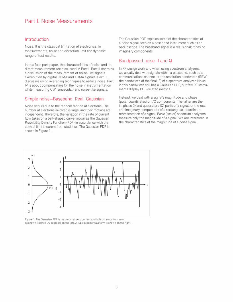
Simple noise—Baseband, Real, GaussianNoise occurs due to the random motion of electrons. The number of electrons involved is large, and their motions are independent. Therefore, the variation in the rate of current flow takes on a bell-shaped curve known as the Gaussian Probability Density Function (PDF) in accordance with the central limit theorem from statistics. The Gaussian PDF is shown in Figure 1.
The Gaussian PDF explains some of the characteristics of a noise signal seen on a baseband instrument such as an oscilloscope. The baseband signal is a real signal; it has no imaginary components.
Bandpassed noise—I and Q
In RF design work and when using spectrum analyzers, we usually deal with signals within a passband, such as a communications channel or the resolution bandwidth (RBW, the bandwidth of the final IF) of a spectrum analyzer. Noise in this bandwidth still has a Gaussian PDF, but few RF instru-ments display PDF-related metrics.
Instead, we deal with a signal’s magnitude and phase (polar coordinates) or I/Q components. The latter are the in-phase (I) and quadrature (Q) parts of a signal, or the real and imaginary components of a rectangular-coordinate representation of a signal. Basic (scalar) spectrum analyzers measure only the magnitude of a signal. We are interested in the characteristics of the magnitude of a noise signal.
Part I: Noise Measurements
3
Figure 1. The Gaussian PDF is maximum at zero current and falls off away from zero, as shown (rotated 90 degrees) on the left. A typical noise waveform is shown on the right.
3
2
1
0
–1
–2
–3
t
3
2
1
0
–1
–2
–3
PDF (i)
ii
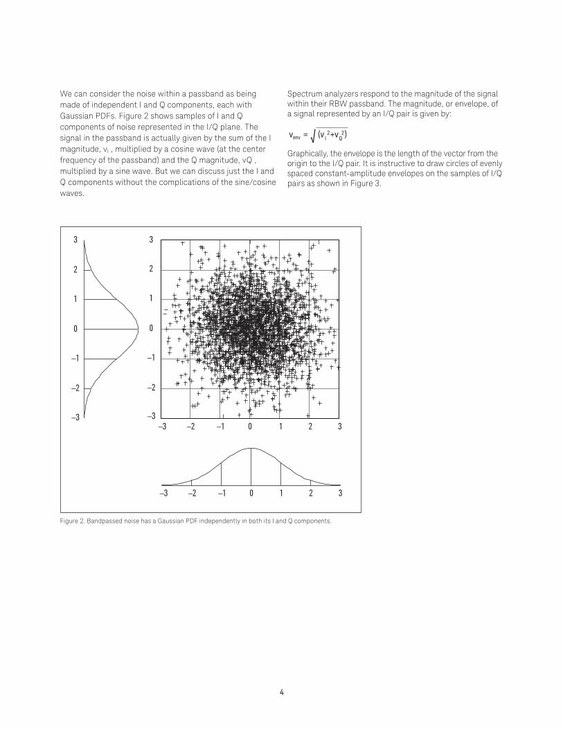
We can consider the noise within a passband as being made of independent I and Q components, each with Gaussian PDFs. Figure 2 shows samples of I and Q components of noise represented in the I/Q plane. The signal in the passband is actually given by the sum of the I magnitude, vI , multiplied by a cosine wave (at the center frequency of the passband) and the Q magnitude, vQ , multiplied by a sine wave. But we can discuss just the I and Q components without the complications of the sine/cosine waves.
Spectrum analyzers respond to the magnitude of the signal within their RBW passband. The magnitude, or envelope, of a signal represented by an I/Q pair is given by:
venv = √ (vI2+vQ
2)
Graphically, the envelope is the length of the vector from the origin to the I/Q pair. It is instructive to draw circles of evenly spaced constant-amplitude envelopes on the samples of I/Q pairs as shown in Figure 3.
Figure 2. Bandpassed noise has a Gaussian PDF independently in both its I and Q components.
–3
–2
–1
0
1
2
3
–3 –2 –1 0 1 2 3
–3 –2 –1 0 1 2 3
–3
–2
–1
0
1
2
3
4
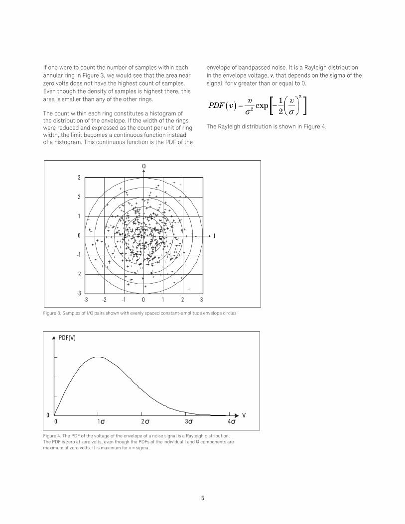
If one were to count the number of samples within each annular ring in Figure 3, we would see that the area near zero volts does not have the highest count of samples. Even though the density of samples is highest there, this area is smaller than any of the other rings.
The count within each ring constitutes a histogram of the distribution of the envelope. If the width of the rings were reduced and expressed as the count per unit of ring width, the limit becomes a continuous function instead of a histogram. This continuous function is the PDF of the
Figure 3. Samples of I/Q pairs shown with evenly spaced constant-amplitude envelope circles
3 2 1 0 1 2 33
2
1
0
1
2
3
Q
I
Figure 4. The PDF of the voltage of the envelope of a noise signal is a Rayleigh distribution. The PDF is zero at zero volts, even though the PDFs of the individual I and Q components are maximum at zero volts. It is maximum for v = sigma.
0 1 2 3 40
PDF(V)
Vσ σ σσ
5
envelope of bandpassed noise. It is a Rayleigh distribution in the envelope voltage, v, that depends on the sigma of the signal; for v greater than or equal to 0.
The Rayleigh distribution is shown in Figure 4.
Measuring the power of noise with an envelope detector
The power of the noise is the parameter we usually want to measure with a spectrum analyzer. The power is the heating value of the signal. Mathematically, it is the time-average of v2(t)/R, where R is the impedance and v(t) is the voltage at time t.
At first glance, we might like to find the average envelope voltage and square it, then divide by R. But finding the square of the average is not the same as finding the average of the square. In fact, there is a consistent under-measurement of noise from squaring the average instead of averaging the square; this under-measurement is 1.05 dB
6
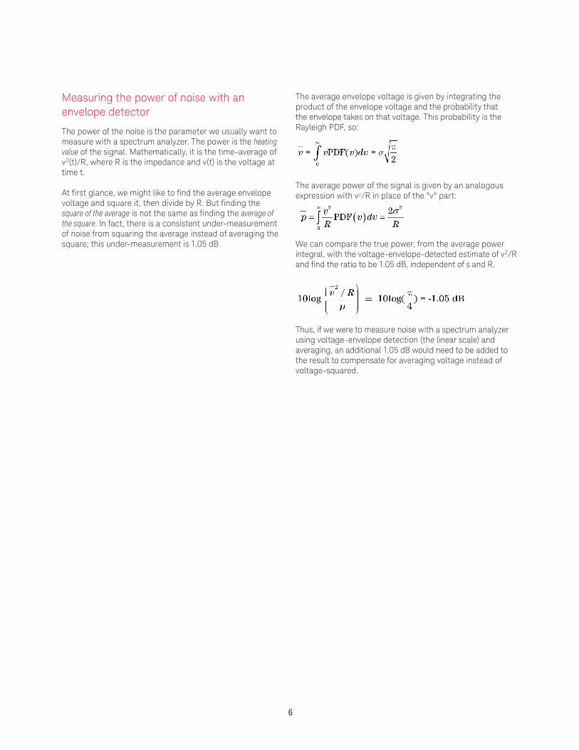
The average envelope voltage is given by integrating the product of the envelope voltage and the probability that the envelope takes on that voltage. This probability is the Rayleigh PDF, so:
The average power of the signal is given by an analogous expression with v2/R in place of the "v" part:
We can compare the true power, from the average power integral, with the voltage-envelope-detected estimate of v2/R and find the ratio to be 1.05 dB, independent of s and R.
Thus, if we were to measure noise with a spectrum analyzer using voltage-envelope detection (the linear scale) and averaging, an additional 1.05 dB would need to be added to the result to compensate for averaging voltage instead of voltage-squared.
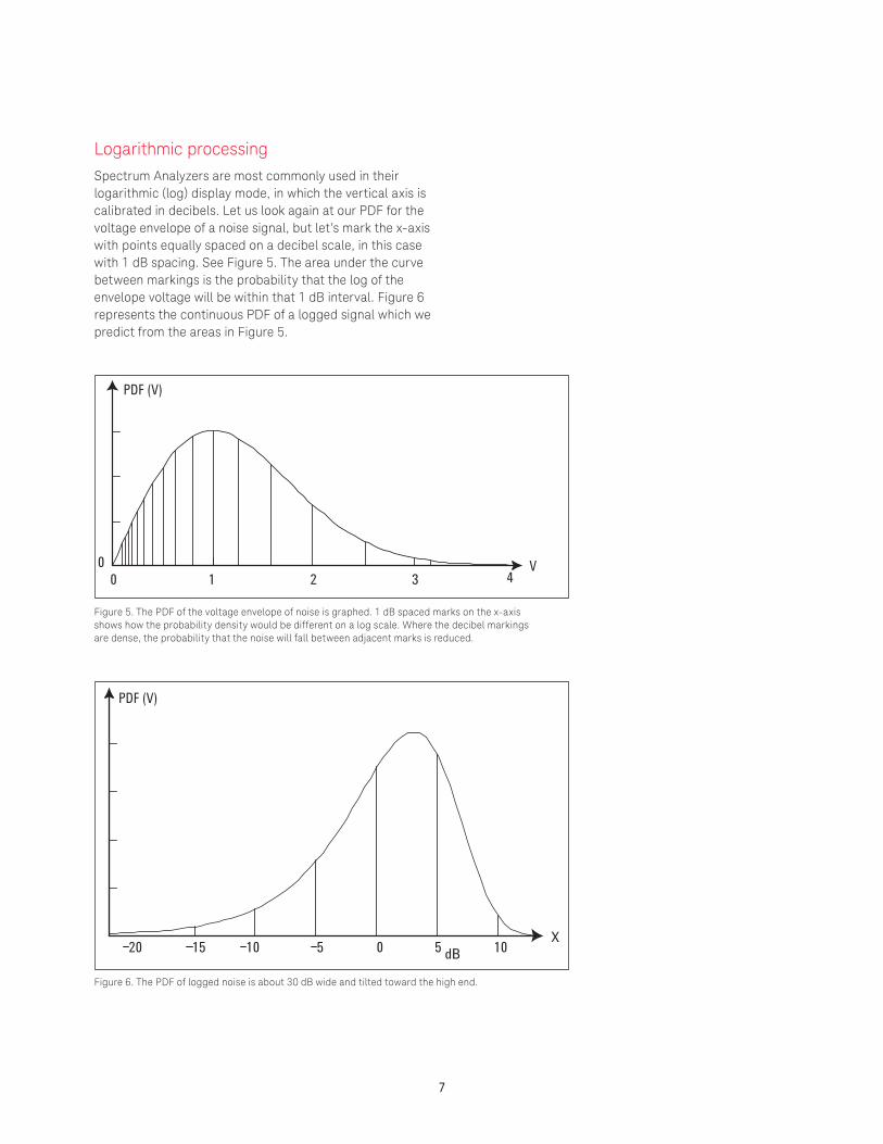
Logarithmic processingSpectrum Analyzers are most commonly used in their logarithmic (log) display mode, in which the vertical axis is calibrated in decibels. Let us look again at our PDF for the voltage envelope of a noise signal, but let’s mark the x-axis with points equally spaced on a decibel scale, in this case with 1 dB spacing. See Figure 5. The area under the curve between markings is the probability that the log of the envelope voltage will be within that 1 dB interval. Figure 6 represents the continuous PDF of a logged signal which we predict from the areas in Figure 5.
Figure 5. The PDF of the voltage envelope of noise is graphed. 1 dB spaced marks on the x-axis shows how the probability density would be different on a log scale. Where the decibel markings are dense, the probability that the noise will fall between adjacent marks is reduced.
Figure 6. The PDF of logged noise is about 30 dB wide and tilted toward the high end.
7
20 15 10 5 0 5 10
PDF (V)
XdB
0 1 2 3 40 V
PDF (V)
Measuring the power of noise with a log-envelope scaleWhen a spectrum analyzer is in a log (dB) display mode, averaging of the results can occur in numerous ways. Multiple traces can be averaged, the envelope can be aver-aged by the action of the video filter, or the noise marker (more on this below) averages results across the x-axis. Some recently introduced analyzers also have a detector that averages the signal amplitude for the duration of a measurement cell.
When we express the average power of the noise in decibels, we compute a logarithm of that average power. When we average the output of the log scale of a spectrum analyzer, we compute the average of the log. The log of the average is not equal to the average of the log. If we go through the same kinds of computations that we did comparing average voltage envelopes with average power envelopes, we find that log processing causes an under-response to noise of 2.51 dB, rather than 1.05 dB.1
The log amplification acts as a compressor for large noise peaks; a peak of ten times the average level is only 10 dB higher. Instantaneous near-zero envelopes, on the other hand, contain no power but are expanded toward negative infinity decibels. The combination of these two aspects of the logarithmic curve causes noise power to measure lower than the true noise power.
Equivalent noise bandwidth
Before discussing the measurement of noise with a spectrum analyzer noise marker, it is necessary to understand the RBW filter of a spectrum analyzer.
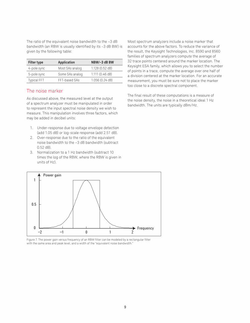
The ideal RBW has a flat passband and infinite attenuation outside that passband. But it must also have good time domain performance so that it behaves well when signals sweep through the passband. Most spectrum analyzers use four-pole synchronously tuned filters for their RBW filters. We can plot the power gain (the square of the voltage gain) of the RBW filter versus frequency as shown in Figure 7. The response of the filter to noise of flat power spectral density will be the same as the response of a rectangular filter with the same maximum gain and the same area under their curves. The width of such a rectangular filter is the equivalent noise bandwidth of the RBW filter. The noise density at the input to the RBW filter is given by the output power divided by the equivalent noise bandwidth.
1. Mostauthorsonthissubjectartificiallystatethatthisfactorisdueto1.05dBfromenvelopedetectionandanother1.45dBfromlogarithmicamplification,reasoningthatthesignalisfirstvoltage-envelopedetected,thenlogarithmicallyamplified.Butifweweretomeasurethevoltage-squaredenvelope(inotherwords,thepowerenvelope,whichwouldcausezeroerrorinsteadof1.05dB)andthenlogit,wewouldstillfinda2.51dBunder-response.Therefore,thereisnorealpointinseparatingthe2.51dBintotwopieces.
8
The ratio of the equivalent noise bandwidth to the –3 dB bandwidth (an RBW is usually identified by its –3 dB BW) is given by the following table:
Filter type Application NBW/–3 dB BW
4-polesync MostSAsanalog 1.128(0.52dB)
5-polesync SomeSAsanalog 1.111(0.46dB)
TypicalFFT FFT-basedSAs 1.056(0.24dB)
The noise markerAs discussed above, the measured level at the output of a spectrum analyzer must be manipulated in order to represent the input spectral noise density we wish to measure. This manipulation involves three factors, which may be added in decibel units:
1. Under-response due to voltage envelope detection (add 1.05 dB) or log-scale response (add 2.51 dB).
2. Over-response due to the ratio of the equivalent noise bandwidth to the –3 dB bandwidth (subtract 0.52 dB).
3. Normalization to a 1 Hz bandwidth (subtract 10 times the log of the RBW, where the RBW is given in units of Hz).
Most spectrum analyzers include a noise marker that accounts for the above factors. To reduce the variance of the result, the Keysight Technologies, Inc. 8590 and 8560 families of spectrum analyzers compute the average of 32 trace points centered around the marker location. The Keysight ESA family, which allows you to select the number of points in a trace, compute the average over one half of a division centered at the marker location. For an accurate measurement, you must be sure not to place the marker too close to a discrete spectral component.
The final result of these computations is a measure of the noise density, the noise in a theoretical ideal 1 Hz bandwidth. The units are typically dBm/Hz.
Figure 7. The power gain versus frequency of an RBW filter can be modeled by a rectangular filter with the same area and peak level, and a width of the “equivalent noise bandwidth.”
2 1 0 1 20
0.5
1Power gain
Frequency
9
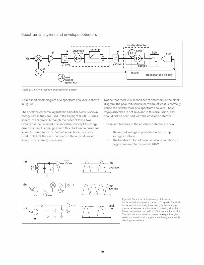
A simplified block diagram of a spectrum analyzer is shown in Figure 8.
The envelope detector/logarithmic amplifier block is shown configured as they are used in the Keysight 8560 E-Series spectrum analyzers. Although the order of these two circuits can be reversed, the important concept to recog-nize is that an IF signal goes into this block and a baseband signal (referred to as the “video” signal because it was used to deflect the electron beam in the original analog spectrum analyzers) comes out.
Notice that there is a second set of detectors in the block diagram: the peak/pit/sample hardware of what is normally called the detector mode of a spectrum analyzer. These display detectors are not relevant to this discussion, and should not be confused with the envelope detector.
The salient features of the envelope detector are two:
1. The output voltage is proportional to the input voltage envelope.
2. The bandwidth for following envelope variations is large compared to the widest RBW.
Figure 8. Simplified spectrum analyzer block diagram
Figure 9. Detectors: a) half-wave, b) full-wave implemented as a “product detector,” c) peak. Practical implementations usually have their gain terms imple-mented elsewhere, and implement buffering after the filters that remove the residual IF carrier and harmonics. The peak detector must be cleared; leakage through a resistor or a switch with appropriate timing are possible clearing mechanisms.
rmspeak
rmsaverage
rmsaverage
(a)
RVinR
(b)Vin
limiter
(c)
x p2
x p22
x21
Vin
processor and display
A/D
sample
log ampenvelopedetector
Vin
LORBW VBW
display detector
peak
sweep generator
S&H
resets
10
Spectrum analyzers and envelope detectors
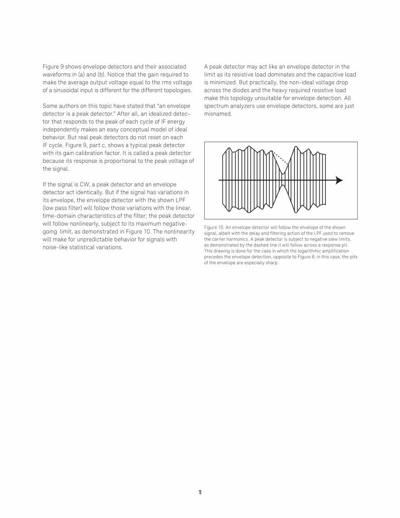
Figure 9 shows envelope detectors and their associated waveforms in (a) and (b). Notice that the gain required to make the average output voltage equal to the rms voltage of a sinusoidal input is different for the different topologies.
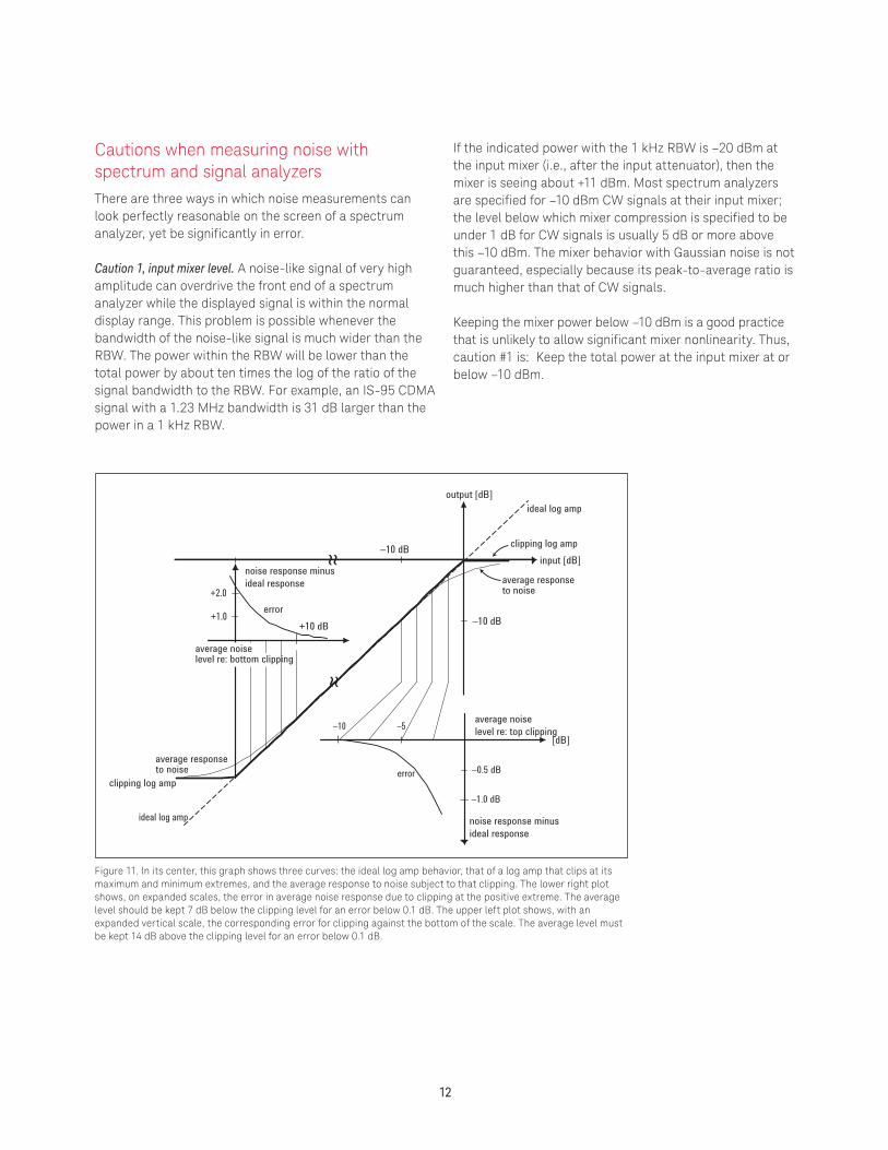
Some authors on this topic have stated that “an envelope detector is a peak detector.” After all, an idealized detec-tor that responds to the peak of each cycle of IF energy independently makes an easy conceptual model of ideal behavior. But real peak detectors do not reset on each IF cycle. Figure 9, part c, shows a typical peak detector with its gain calibration factor. It is called a peak detector because its response is proportional to the peak voltage of the signal. If the signal is CW, a peak detector and an envelope detector act identically. But if the signal has variations in its envelope, the envelope detector with the shown LPF (low pass filter) will follow those variations with the linear, time-domain characteristics of the filter; the peak detector will follow nonlinearly, subject to its maximum negative-going limit, as demonstrated in Figure 10. The nonlinearity will make for unpredictable behavior for signals with noise-like statistical variations.
A peak detector may act like an envelope detector in the limit as its resistive load dominates and the capacitive load is minimized. But practically, the non-ideal voltage drop across the diodes and the heavy required resistive load make this topology unsuitable for envelope detection. All spectrum analyzers use envelope detectors, some are just misnamed.
Figure 10. An envelope detector will follow the envelope of the shown signal, albeit with the delay and filtering action of the LPF used to remove the carrier harmonics. A peak detector is subject to negative slew limits, as demonstrated by the dashed line it will follow across a response pit. This drawing is done for the case in which the logarithmic amplification precedes the envelope detection, opposite to Figure 8; in this case, the pits of the envelope are especially sharp.
11
Cautions when measuring noise with spectrum and signal analyzersThere are three ways in which noise measurements can look perfectly reasonable on the screen of a spectrum analyzer, yet be significantly in error.
Caution 1, input mixer level. A noise-like signal of very high amplitude can overdrive the front end of a spectrum analyzer while the displayed signal is within the normal display range. This problem is possible whenever the bandwidth of the noise-like signal is much wider than the RBW. The power within the RBW will be lower than the total power by about ten times the log of the ratio of the signal bandwidth to the RBW. For example, an IS-95 CDMA signal with a 1.23 MHz bandwidth is 31 dB larger than the power in a 1 kHz RBW.
If the indicated power with the 1 kHz RBW is –20 dBm at the input mixer (i.e., after the input attenuator), then the mixer is seeing about +11 dBm. Most spectrum analyzers are specified for –10 dBm CW signals at their input mixer; the level below which mixer compression is specified to be under 1 dB for CW signals is usually 5 dB or more above this –10 dBm. The mixer behavior with Gaussian noise is not guaranteed, especially because its peak-to-average ratio is much higher than that of CW signals.
Keeping the mixer power below –10 dBm is a good practice that is unlikely to allow significant mixer nonlinearity. Thus, caution #1 is: Keep the total power at the input mixer at or below –10 dBm.
Figure 11. In its center, this graph shows three curves: the ideal log amp behavior, that of a log amp that clips at its maximum and minimum extremes, and the average response to noise subject to that clipping. The lower right plot shows, on expanded scales, the error in average noise response due to clipping at the positive extreme. The average level should be kept 7 dB below the clipping level for an error below 0.1 dB. The upper left plot shows, with an expanded vertical scale, the corresponding error for clipping against the bottom of the scale. The average level must be kept 14 dB above the clipping level for an error below 0.1 dB.
+2.0
+1.0+10 dB
noise response minusideal response
average noiselevel re: bottom clipping
average responseto noise
clipping log amp
ideal log amp
≈ input [dB]
average response to noise
clipping log amp
ideal log amp
error
–10 –5
–0.5 dB
–10 dB
–1.0 dB
average noiselevel re: top clipping
[dB]
noise response minusideal response
error
output [dB]
–10 dB
≈
12
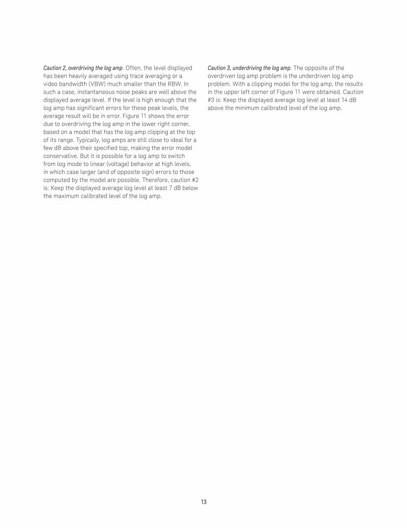
Caution 2, overdriving the log amp. Often, the level displayed has been heavily averaged using trace averaging or a video bandwidth (VBW) much smaller than the RBW. In such a case, instantaneous noise peaks are well above the displayed average level. If the level is high enough that the log amp has significant errors for these peak levels, the average result will be in error. Figure 11 shows the error due to overdriving the log amp in the lower right corner, based on a model that has the log amp clipping at the top of its range. Typically, log amps are still close to ideal for a few dB above their specified top, making the error model conservative. But it is possible for a log amp to switch from log mode to linear (voltage) behavior at high levels, in which case larger (and of opposite sign) errors to those computed by the model are possible. Therefore, caution #2 is: Keep the displayed average log level at least 7 dB below the maximum calibrated level of the log amp.
Caution 3, underdriving the log amp. The opposite of the overdriven log amp problem is the underdriven log amp problem. With a clipping model for the log amp, the results in the upper left corner of Figure 11 were obtained. Caution #3 is: Keep the displayed average log level at least 14 dB above the minimum calibrated level of the log amp.
13
In Part I, we discussed the characteristics of noise and its measurement. In this part, we will discuss three different measurements of digitally modulated signals, after showing why they are very much like noise.
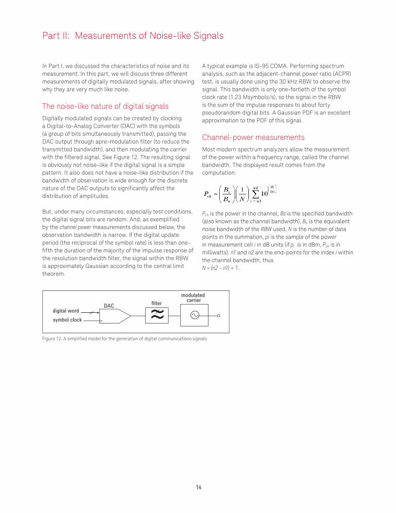
The noise-like nature of digital signalsDigitally modulated signals can be created by clocking a Digital-to-Analog Converter (DAC) with the symbols (a group of bits simultaneously transmitted), passing the DAC output through apre-modulation filter (to reduce the transmitted bandwidth), and then modulating the carrier with the filtered signal. See Figure 12. The resulting signal is obviously not noise-like if the digital signal is a simple pattern. It also does not have a noise-like distribution if the bandwidth of observation is wide enough for the discrete nature of the DAC outputs to significantly affect the distribution of amplitudes.
But, under many circumstances, especially test conditions, the digital signal bits are random. And, as exemplified by the channel power measurements discussed below, the observation bandwidth is narrow. If the digital update period (the reciprocal of the symbol rate) is less than one-fifth the duration of the majority of the impulse response of the resolution bandwidth filter, the signal within the RBW is approximately Gaussian according to the central limit theorem.
A typical example is IS-95 CDMA. Performing spectrum analysis, such as the adjacent-channel power ratio (ACPR) test, is usually done using the 30 kHz RBW to observe the signal. This bandwidth is only one-fortieth of the symbol clock rate (1.23 Msymbols/s), so the signal in the RBW is the sum of the impulse responses to about forty pseudorandom digital bits. A Gaussian PDF is an excellent approximation to the PDF of this signal.
Channel-power measurements Most modern spectrum analyzers allow the measurement of the power within a frequency range, called the channel bandwidth. The displayed result comes from the computation:
Pch is the power in the channel, Bs is the specified bandwidth (also known as the channel bandwidth), Bn is the equivalent noise bandwidth of the RBW used, N is the number of data points in the summation, pi is the sample of the power in measurement cell i in dB units (if pi is in dBm, Pch is in milliwatts). n1 and n2 are the end-points for the index i within the channel bandwidth, thus N = (n2 – n1) + 1.
Part II: Measurements of Noise-like Signals
Figure 12. A simplified model for the generation of digital communications signals.
14
DAC filtermodulated
carrier
≈digital wordsymbol clock
The computation works well for CW signals, such as from sinusoidal modulation. The computation is a power-summing computation. Because the computation changes the input data points to a power scale before summing, there is no need to compensate for the difference between the log of the average and the average of the log as explained in Part I, even if the signal has a noise-like PDF (probability density function). But, if the signal starts with noise-like statistics and is averaged in decibel form (typically with a VBW filter on the log scale) before the power summation, some 2.51 dB under-response, as explained in Part I, will be incurred. If we are certain that the signal is of noise-like statistics, and we fully average the signal before performing the summation, we can add 2.51 dB to the result and have an accurate measurement. Furthermore, the averaging reduces the variance of the result.
But if we don’t know the statistics of the signal, the best measurement technique is to do no averaging before power summation. Using a VBW ≥ 3RBW is required for insignificant averaging, and is thus recommended. But the bandwidth of the video signal is not as obvious as it appears. In order to not peak-bias the measurement, the sample detector must be used. Spectrum analyzers have lower
effective video bandwidths in sample detection than they do in peak detection mode, because of the limitations of the sample-and-hold circuit that precedes the A/D converter. Examples include the Keysight 8560E-Series spectrum analyzer family with 450 kHz effective sample-mode video bandwidth, and a substantially wider bandwidth (over 2 MHz) in the Keysight ESA-E Series spectrum analyzer family.
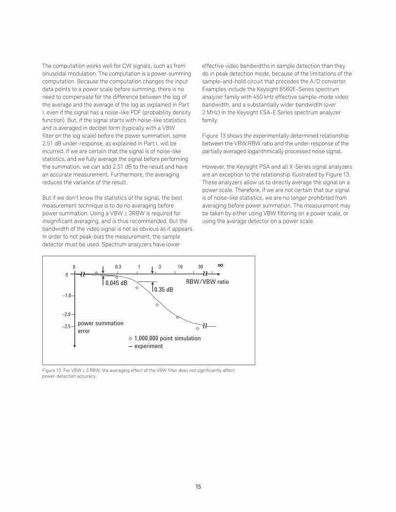
Figure 13 shows the experimentally determined relationship between the VBW:RBW ratio and the under-response of the partially averaged logarithmically processed noise signal.
However, the Keysight PSA and all X-Series signal analyzers are an exception to the relationship illustrated by Figure 13. These analyzers allow us to directly average the signal on a power scale. Therefore, if we are not certain that our signal is of noise-like statistics, we are no longer prohibited from averaging before power summation. The measurement may be taken by either using VBW filtering on a power scale, or using the average detector on a power scale.
Figure 13. For VBW ≥ 3 RBW, the averaging effect of the VBW filter does not significantly affect power-detection accuracy.
15
00
0.3 1 3 10 30 ∞
≈
≈≈
–1.0
–2.0
–2.5 power summationerror
0.045 dB
1,000,000 point simulation experiment
RBW/VBW ratio0.35 dB
Adjacent-Channel Power (ACP)There are many standards for the measurement of ACP with a spectrum analyzer. The issues involved in most ACP measurements are covered in detail in an article in Microwaves & RF, May, 1992, "Make Adjacent-Channel Power Measurements." A survey of other standards is available in "Adjacent Channel Power Measurements in the Digital Wireless Era" in Microwave Journal, July, 1994.
For digitally modulated signals, ACP and channel-power measurements are similar, except ACP is easier. ACP is usually the ratio of the power in the main channel to the power in an adjacent channel. If the modulation is digital, the main channel will have noise-like statistics. Whether the signals in the adjacent channel are due to broadband noise, phase noise, or intermodulation of noise-like signals in the main channel, the adjacent channel will have noise-like statistics. A spurious signal in the adjacent channel is most likely modulated to appear noise-like, too, but a CW-like tone is a possibility.
If the main and adjacent channels are both noise-like, then their ratio will be accurately measured regardless of whether their true power or log-averaged power (or any partially averaged result between these extremes) is measured. Thus, unless discrete CW tones are found in the signals, ACP is not subject to the cautions regarding VBW and other averaging noted in the section on channel power above.
But some ACP standards call for the measurement of absolute power, rather than a power ratio. In such cases, the cautions about VBW and other averaging do apply.
Carrier powerBurst carriers, such as those used in TDMA mobile stations, are measured differently than continuous carriers. The power of the transmitter during the time it is on is called the "carrier power."
Carrier power is measured with the spectrum analyzer in zero span. In this mode, the LO of the analyzer does not sweep, thus the span swept is zero. The display then shows amplitude normally on the y axis, and time on the x axis. If we set the RBW large compared to the bandwidth of the burst signal, then all of the display points include all of the power in the channel. The carrier power is computed simply by averaging the power of all the display points that represent the times when the burst is on. Depending on the modulation type, this is often considered to be any point within 20 dB of the highest registered amplitude. (A trigger and gated spectrum analysis may be used if the carrier power is to be measured over a specified portion of a burst-RF signal.)
Using a wide RBW for the carrier-power measurement means that the signal will not have noise-like statistics. It will not have CW-like statistics, either, so it is still wise to set the VBW as wide as possible. But let’s consider some examples to see if the sample-mode bandwidths of spectrum analyzers are a problem.
For PDC, NADC and TETRA, the symbol rates are under 25 kb/s, so a VBW set to maximum will work well. It will also work well for PHS and GSM, with symbol rates of 380 and 270 kb/s. For IS-95 CDMA, with a modulation rate of 1.23 MHz, we could anticipate a problem with the 450 kHz effective video bandwidth discussed in the section on channel power above. Experimentally, an instrument with 450 kHz BW experienced a 0.6 dB error with an OQPSK (mobile) burst signal.
16
17
Peak-detected noise and TDMA ACP measurementsTDMA (time-division multiple access, or burst-RF) systems are usually measured with peak detectors, in order that the burst "off" events are not shown on the screen of the spectrum analyzer, potentially distracting the user. Examples include ACP measurements for PDC (Personal Digital Cel-lular) by two different methods, PHS (Personal Handiphone System) and NADC (North American Dual-mode Cellular). Noise is also often peak detected in the measurement of rotating media, such as hard disk drives and VCRs.
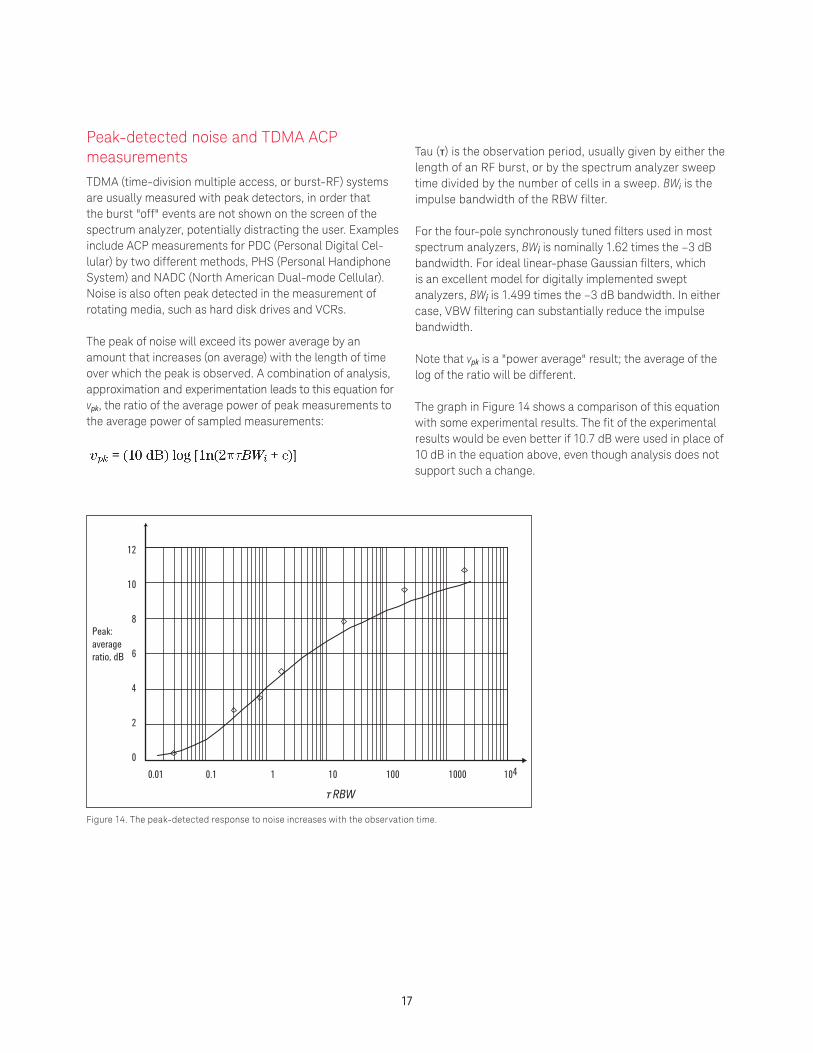
The peak of noise will exceed its power average by an amount that increases (on average) with the length of time over which the peak is observed. A combination of analysis, approximation and experimentation leads to this equation for vpk, the ratio of the average power of peak measurements to the average power of sampled measurements:
Tau (т) is the observation period, usually given by either the length of an RF burst, or by the spectrum analyzer sweep time divided by the number of cells in a sweep. BWi is the impulse bandwidth of the RBW filter.
For the four-pole synchronously tuned filters used in most spectrum analyzers, BWi is nominally 1.62 times the –3 dB bandwidth. For ideal linear-phase Gaussian filters, which is an excellent model for digitally implemented swept analyzers, BWi is 1.499 times the –3 dB bandwidth. In either case, VBW filtering can substantially reduce the impulse bandwidth.
Note that vpk is a "power average" result; the average of the log of the ratio will be different.
The graph in Figure 14 shows a comparison of this equation with some experimental results. The fit of the experimental results would be even better if 10.7 dB were used in place of 10 dB in the equation above, even though analysis does not support such a change.
Figure 14. The peak-detected response to noise increases with the observation time.
0.01 0.1 1 10 100 1000 104
12
10
8
6
4
2
0
Peak: average ratio, dB
τ RBWт RBW
18
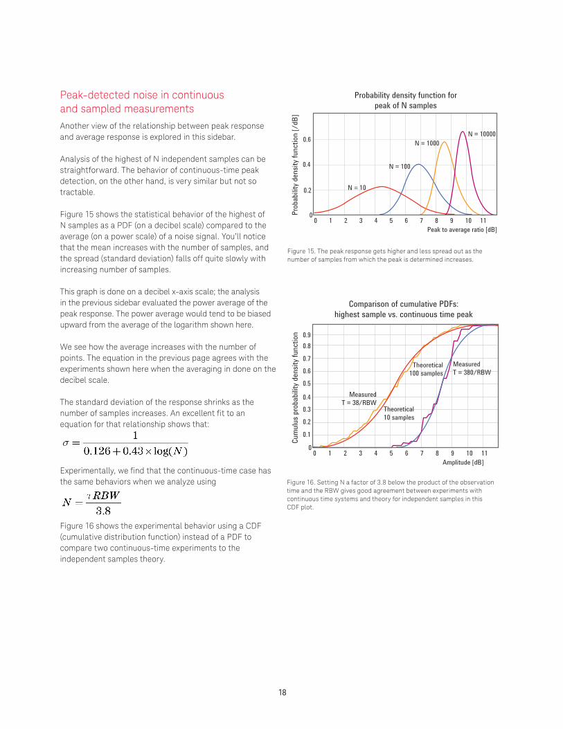
Peak-detected noise in continuous and sampled measurementsAnother view of the relationship between peak response and average response is explored in this sidebar.
Analysis of the highest of N independent samples can be straightforward. The behavior of continuous-time peak detection, on the other hand, is very similar but not so tractable.
Figure 15 shows the statistical behavior of the highest of N samples as a PDF (on a decibel scale) compared to the average (on a power scale) of a noise signal. You’ll notice that the mean increases with the number of samples, and the spread (standard deviation) falls off quite slowly with increasing number of samples.
This graph is done on a decibel x-axis scale; the analysis in the previous sidebar evaluated the power average of the peak response. The power average would tend to be biased upward from the average of the logarithm shown here.
We see how the average increases with the number of points. The equation in the previous page agrees with the experiments shown here when the averaging in done on the decibel scale.
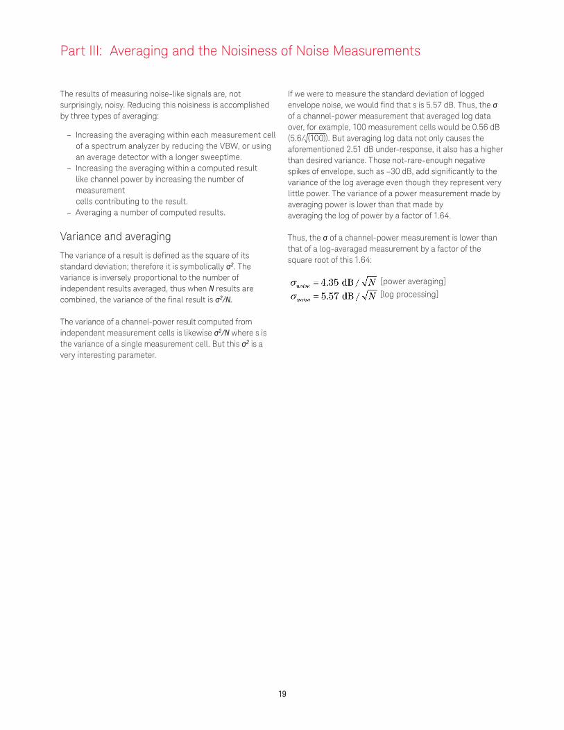
The standard deviation of the response shrinks as the number of samples increases. An excellent fit to an equation for that relationship shows that:
Experimentally, we find that the continuous-time case has the same behaviors when we analyze using
Figure 16 shows the experimental behavior using a CDF (cumulative distribution function) instead of a PDF to compare two continuous-time experiments to the independent samples theory.
Figure 15. The peak response gets higher and less spread out as the number of samples from which the peak is determined increases.
Probability density function for peak of N samples
Peak to average ratio [dB]0 1 2 3 4 5 6 7 8 9 10 11
0.6
0.4
0.2
0Prob
abilit
y den
sity f
unct
ion
[/dB
]
N = 10000N = 1000
N = 100
N = 10
Comparison of cumulative PDFs: highest sample vs. continuous time peak
Amplitude [dB]0 1 2 3 4 5 6 7 8 9 10 11
0.6
0.4
0.2
0.3
0.5
0.7
0.80.9
0.1
0
Cum
ulus
pro
babi
lity d
ensit
y fun
ctio
n
Measured T = 38/RBW
Theoretical10 samples
MeasuredT = 380/RBW
Theoretical100 samples
Figure 16. Setting N a factor of 3.8 below the product of the observation time and the RBW gives good agreement between experiments with continuous time systems and theory for independent samples in this CDF plot.
19
The results of measuring noise-like signals are, not surprisingly, noisy. Reducing this noisiness is accomplished by three types of averaging:
– Increasing the averaging within each measurement cell of a spectrum analyzer by reducing the VBW, or using an average detector with a longer sweeptime.
– Increasing the averaging within a computed result like channel power by increasing the number of measurement cells contributing to the result.
– Averaging a number of computed results.
Variance and averaging
The variance of a result is defined as the square of its standard deviation; therefore it is symbolically σ2. The variance is inversely proportional to the number of independent results averaged, thus when N results are combined, the variance of the final result is σ2/N.
The variance of a channel-power result computed from independent measurement cells is likewise σ2/N where s is the variance of a single measurement cell. But this σ2 is a very interesting parameter.
Part III: Averaging and the Noisiness of Noise Measurements
If we were to measure the standard deviation of logged envelope noise, we would find that s is 5.57 dB. Thus, the σ of a channel-power measurement that averaged log data over, for example, 100 measurement cells would be 0.56 dB (5.6/√(100)). But averaging log data not only causes the aforementioned 2.51 dB under-response, it also has a higher than desired variance. Those not-rare-enough negative spikes of envelope, such as –30 dB, add significantly to the variance of the log average even though they represent very little power. The variance of a power measurement made by averaging power is lower than that made by averaging the log of power by a factor of 1.64.
Thus, the σ of a channel-power measurement is lower than that of a log-averaged measurement by a factor of the square root of this 1.64:
[power averaging]
[log processing]
20
Averaging a number of computed resultsIf we average individual channel-power measurements to get a lower-variance final estimate, we do not have to convert dB-format answers to absolute power to get the advantages of avoiding log averaging. The individual measurements, being the results of many measurement cells summed together, no longer have a distribution like the "logged Rayleigh" but rather look Gaussian. Also, their distribution is sufficiently narrow that the log (dB) scale is linear enough to be a good approximation of the power scale. Thus, we can dB-average our intermediate results.
Swept versus FFT analysisIn the above discussion, we have assumed that the variance reduced by a factor of N was of independent results. This independence is typically the case in swept-spectrum analyzers, due to the time required to sweep from one measurement cell to the next under typical conditions of span, RBW and sweep time. FFT analyzers will usually have many fewer independent points in a measurement across a channel bandwidth, reducing, but not eliminating, their theoretical speed advantage for true noise signals.
For digital communications signals, FFT analyzers have an even greater speed advantage than their throughput predicts. Consider a constant-envelope modulation, such as used in GSM cellular phones. The constant-envelope modulation means that the measured power will be constant when that power is measured over a bandwidth wide enough to include all the power. FFT analysis made in a wide span will allow channel power measurements with very low variance.
But swept analysis will typically be performed with an RBW much narrower than the symbol rate. In this case, the spectrum looks noise-like, and channel power measure-ments will have a higher variance that is not influenced by the constant amplitude nature of the modulation.
Zero spanA zero-span measurement of carrier power is made with a wide RBW, so the independence of data points is determined by the symbol rate of the digital modulation. Data points spaced by a time greater than the symbol rate will be almost completely independent.
Zero span is sometimes used for other noise and noise-like measurements where the noise bandwidth is much greater than the RBW, such as in the measurement of power spectral
density. For example, some companies specify IS-95 CDMA ACPR measurements that are spot-frequency power spectral density specifications; zero span can be used to speed this kind of measurement.
Averaging with an average detectorWith an averaging detector the amplitude of the signal envelope is averaged during the time and frequency interval of a measurement cell. An improvement over using sample detection for summation, the average detector changes the summation over a range of cells into integration over the time interval representing a range of frequencies. The integration thereby captures all power information, not just that sampled by the sample detector.
The primary application of average detection may be seen in the channel power and ACP measurements, discussed in Part II.
Measuring the power of noise with a power envelope scale
The averaging detector is valuable in making integrated power measurements. The averaging scale, when au-tocoupled, is determined by such parameters as the marker function, detection mode and display scale. We have discussed circumstances that may require the use of the log-envelope and voltage envelope scales, now we may consider the power scale.
When making a power measurement, we must remember that traditional swept spectrum analyzers average the log of the envelope when the display is in log mode. As previously mentioned, the log of the average is not equal to the average of the log. Therefore, when making power measurements, it is important to average the power of the signal, or equivalently, to report the root of the mean of the square (rms) number of the signal. With the Keysight PSA analyzer, an "Avg/VBW Type" key allows for manual selection, as well as automatic selection, of the averaging scale (log scale, voltage scale, or power scale; on Keysight X-Series analyzers, the key is named "Average Type. The averaging scale and display scale may be completely independent of each other.
21
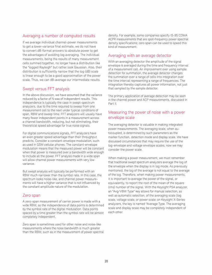
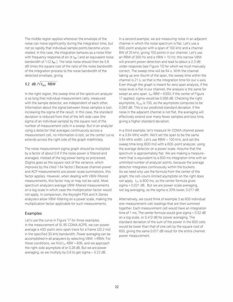
The standard deviation of measurement noiseFigure 17 summarizes the standard deviation of the measurement of noise. The figure represents the standard deviation of the measurement of a noise-like signal using a spectrum analyzer in zero span, averaging the results across the entire screen width, using the log scale. is the integration time (sweep time). The curve is also useful for swept spectrum measurements, such as channel-power measurements. There are three regions to the curve.
The left region applies whenever the integration time is short compared to the rate of change of the noise envelope.
As discussed above, without VBW filtering, the σ is 5.6 dB. When video filtering is applied, the standard deviation is im-proved by a factor. That factor is the square root of the ratio of the two noise bandwidths: that of the video bandwidth, to that of the detected envelope of the noise. The detected envelope of the noise has half the noise bandwidth of the undetected noise. For the four-pole synchronously tuned filters typical of most spectrum analyzers, the detected envelope has a noise bandwidth of (1/2) x 1.128 times the RBW. The noise bandwidth of a single-pole VBW filter is π/2 times its bandwidth. Gathering terms together yields the equation:
Figure 17. Noise measurement standard deviation for log-response (see text for power-response) spectrum analysis depends on the product of the sweep time and RBW, the ratio of the VBW to RBW, and the number of display cells.
1.0 10 100 1k 10k
center curve:5.2 dB
tINT . RBW
5.6 dB
1.0 dB
0.1 dB
≈
≈
[left asymptote]Ncells
N=400N=600
VBW = ∞
VBW = 0.03 . RBW
left asymptote: for VBW >1/3 RBW: 5.6 dB for VBW ≤ 1/3 RBW: 9.3 dB VBW
RBW
tINT . RBW
N=600,VBW=0.03 . RBW
Average detector, any N
σ
right asymptote:
22
The middle region applies whenever the envelope of the noise can move significantly during the integration time, but not so rapidly that individual sample points become uncor-related. In this case, the integration behaves as a noise filter with frequency response of sin (π tINT ) and an equivalent noise bandwidth of 1/(2 tINT ). The total noise should then be 5.6 dB times the square root of the ratio of the noise bandwidth of the integration process to the noise bandwidth of the detected envelope, giving
5.2 dB /√tINT RBW
In the right region, the sweep time of the spectrum analyzer is so long that individual measurement cells, measured with the sample detector, are independent of each other. Information about the signal between these samples is lost, increasing the sigma of the result. In this case, the standard deviation is reduced from that of the left-side case (the sigma of an individual sample) by the square root of the number of measurement cells in a sweep. But in an analyzer using a detector that averages continuously across a measurement cell, no information is lost, so the center curve extends across the right side of the graph indefinitely.
The noise measurement sigma graph should be multiplied by a factor of about 0.8 if the noise power is filtered and averaged, instead of the log power being so processed. (Sigma goes as the square root of the variance, which improves by the cited 1.64 factor.) Because channel-power and ACP measurements are power-scale summations, this factor applies. However, when dealing with VBW-filtered measurements, this factor may or may not be valid. Most spectrum analyzers average VBW-filtered measurements on a log scale in which case the multiplication factor would not apply. In comparison, the Keysight PSA and X-Series analyzers allow VBW-filtering on a power scale, making the multiplication factor applicable for such measurements.
Examples
Let’s use the curve in Figure 17 for three examples. In the measurement of IS-95 CDMA ACPR, we can power-average a 400-point zero-span trace for a frame (20.2 ms) in the specified 30 kHz bandwidth. Power averaging can be accomplished in all analyzers by selecting VBW >>RBW. For these conditions, we find tINT RBW = 606, and we approach the right-side asymptote of or 0.28 dB. But we are power averaging, so we multiply by 0.8 to get sigma = 0.22 dB.
In a second example, we are measuring noise in an adjacent channel in which the noise spectrum is flat. Let’s use a 600-point analyzer with a span of 100 kHz and a channel BW of 25 kHz, giving 150 points in our channel. Let’s use an RBW of 300 Hz and a VBW = 10 Hz; this narrow VBW will prevent power detection and lead to about a 2.3 dB under-response (see Figure 13) for which we must manually correct. The sweep time will be 84 s. With the channel taking up one-fourth of the span, the sweep time within the channel is 21 s, so that is the integration time for our x-axis. Even though the graph is meant for zero span analysis, if the noise level is flat in our channel, the analysis is the same for swept as zero span. tINT RBW = 6300; if the center of Figure 17 applied, sigma would be 0.066 dB. Checking the right asymptote, Ncells is 150, so the asymptote computes to be 0.083 dB. This is our predicted standard deviation. If the noise in the adjacent channel is not flat, the averaging will effectively extend over many fewer samples and less time, giving a higher standard deviation.
In a third example, let’s measure W-CDMA channel power in a 3.84 MHz width. We’ll set the span to be the same 3.84 MHz width. Let’s use RBW = 100 kHz, and set the sweep time long (600 ms) with a 600-point analyzer, using the average detector on a power scale. Assume that the spectrum is approximately flat. We are making a measure-ment that is equivalent to a 600 ms integration time with an unlimited number of analyzer points, because the average detector integrates continuously within the buckets. So we need only use the formula from the center of the graph; the cell-count-limited asymptote on the right does not apply. tINT is 600 ms, so the center formula gives sigma = 0.021 dB. But we are power-scale averaging, not log averaging, so the sigma is 20% lower, 0.017 dB.
Alternatively, we could think of example 3 as 600 individual one-measurement-cell readings that are then summed together. Each measurement cell would have an integration time of 1 ms. The center formula would give sigma = 0.52 dB on a log scale, or 0.412 dB for power averaging. The standard deviation of the sum of the power in the 600 cells would be lower than that of one cell by the square root of 600, giving the same 0.017 dB result for the entire channel power measurement.
23
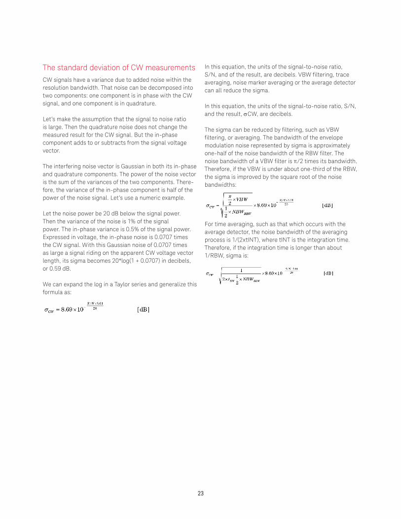
The standard deviation of CW measurementsCW signals have a variance due to added noise within the resolution bandwidth. That noise can be decomposed into two components: one component is in phase with the CW signal, and one component is in quadrature.
Let’s make the assumption that the signal to noise ratio is large. Then the quadrature noise does not change the measured result for the CW signal. But the in-phase component adds to or subtracts from the signal voltage vector.
The interfering noise vector is Gaussian in both its in-phase and quadrature components. The power of the noise vector is the sum of the variances of the two components. There-fore, the variance of the in-phase component is half of the power of the noise signal. Let’s use a numeric example.
Let the noise power be 20 dB below the signal power. Then the variance of the noise is 1% of the signal power. The in-phase variance is 0.5% of the signal power. Expressed in voltage, the in-phase noise is 0.0707 times the CW signal. With this Gaussian noise of 0.0707 times as large a signal riding on the apparent CW voltage vector length, its sigma becomes 20*log(1 + 0.0707) in decibels, or 0.59 dB.
We can expand the log in a Taylor series and generalize this formula as:
In this equation, the units of the signal-to-noise ratio, S/N, and of the result, are decibels. VBW filtering, trace averaging, noise marker averaging or the average detector can all reduce the sigma.
In this equation, the units of the signal-to-noise ratio, S/N, and the result, σCW, are decibels.
The sigma can be reduced by filtering, such as VBW filtering, or averaging. The bandwidth of the envelope modulation noise represented by sigma is approximately one-half of the noise bandwidth of the RBW filter. The noise bandwidth of a VBW filter is π/2 times its bandwidth. Therefore, if the VBW is under about one-third of the RBW, the sigma is improved by the square root of the noise bandwidths:
For time averaging, such as that which occurs with the average detector, the noise bandwidth of the averaging process is 1/(2xtINT), where tINT is the integration time. Therefore, if the integration time is longer than about 1/RBW, sigma is:
24
Part IV: Compensation for Instrumentation Noise
In Parts I, II and III, we discussed the measurement of noise and noise-like signals respectively. In this part, we’ll discuss measuring CW and noise-like signals in the presence of instrumentation noise. We’ll see why averaging the output of a logarithmic amplifier is optimum for CW measurements, and we’ll review compensation formulas for removing known noise levels from noise-plus-signal measurements.
CW signals and log versus power detection
When measuring a single CW tone in the presence of noise, and using power detection, the level measured is equal to the sum of the power of the CW tone and the power of the noise within the RBW filter. Thus, we could improve the accuracy of a measurement by measuring the CW tone first (let’s call this the "S+N" or signal-plus-noise), then disconnect the signal to make the "N" measurement. The difference between the two, with both measurements in power units (for example, milliwatts, not dBm) would be the signal power.
But measuring with a log scale and video filtering or video averaging results in unexpectedly good results. As described in Part I, the noise will be measured lower than a CW signal with equal power within the RBW by 2.5 dB. But to the first order, the noise doesn’t even affect the S+N measurement! See "Log Scale Ideal for CW Measurements" later in this section.
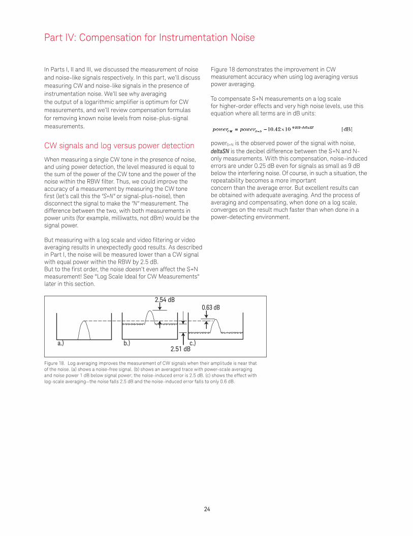
Figure 18 demonstrates the improvement in CW measurement accuracy when using log averaging versus power averaging.
To compensate S+N measurements on a log scale for higher-order effects and very high noise levels, use this equation where all terms are in dB units:
powerS+N is the observed power of the signal with noise, deltaSN is the decibel difference between the S+N and N-only measurements. With this compensation, noise-induced errors are under 0.25 dB even for signals as small as 9 dB below the interfering noise. Of course, in such a situation, the repeatability becomes a more important concern than the average error. But excellent results can be obtained with adequate averaging. And the process of averaging and compensating, when done on a log scale, converges on the result much faster than when done in a power-detecting environment.
Figure 18. Log averaging improves the measurement of CW signals when their amplitude is near that of the noise. (a) shows a noise-free signal. (b) shows an averaged trace with power-scale averaging and noise power 1 dB below signal power; the noise-induced error is 2.5 dB. (c) shows the effect with log-scale averaging—the noise falls 2.5 dB and the noise-induced error falls to only 0.6 dB.
a.) b.) c.)
2.54 dB0.63 dB
2.51 dB
25
Power-detection measurements and noise subtractionIf the signal to be measured has the same statistical distribution as the instrumentation noise— in other words, if the signal is noise-like—then the sum of the signal and instrumentation noise will be a simple power sum:
Note that the units of all variables must be power units such as milliwatts and not log units like dBm, nor voltage units like mV. Note also that this equation applies even if powerS and powerN are measured with log averaging.
The power equation also applies when the signal and the noise have different statistics (CW and Gaussian respectively) but power detection is used. The power equation would never apply if the signal and the noise were correlated, either in-phase adding or subtracting. But that will never be the case with noise.
Therefore, simply enough, we can subtract the measured noise power from any power-detected result to get improved accuracy. Results of interest are the channel-power, ACP, and carrier-power measurements described in Part II. The equation would be:
Care should be exercised that the measurement setups for powerN and powerS+N are as similar as possible. When the input attenuation is at or near 0 dB, it will be important to terminate the input for the powerN case.
Noise subtraction can be done inside the analyzer in the most modern spectrum analyzers from Keysight. They have the “Power Diff” trace math function available.
Noise Floor Extension (NFE) for noise compensation A very convenient form of noise compensation is now built-in to some advanced spectrum analyzers: NFE. It goes beyond the power subtraction we just discussed.
NFE creates a model of the noise of the spectrum analyzer as a function of its state. This model works for all RBWs, all attenuation settings, all paths (such as preamp on and off), even all detectors (such as peak and average) and VBW settings. The user does not need to characterize his analyzer before turning NFE on, because the models are already in the analyzer.
NFE is most effective with noise-like signals, but it also works on CW and impulsive signals. It greatly reduces the errors caused by noise, replacing them with a smaller uncertainty. See the reference “Using Noise Floor Extension in the PXA Signal Analyzer” for more information on this topic.
NFE can often allow the user to see signals below the theoretical noise floor of a room-temperature termination impedance. See the reference for discussion on that topic, too.
26
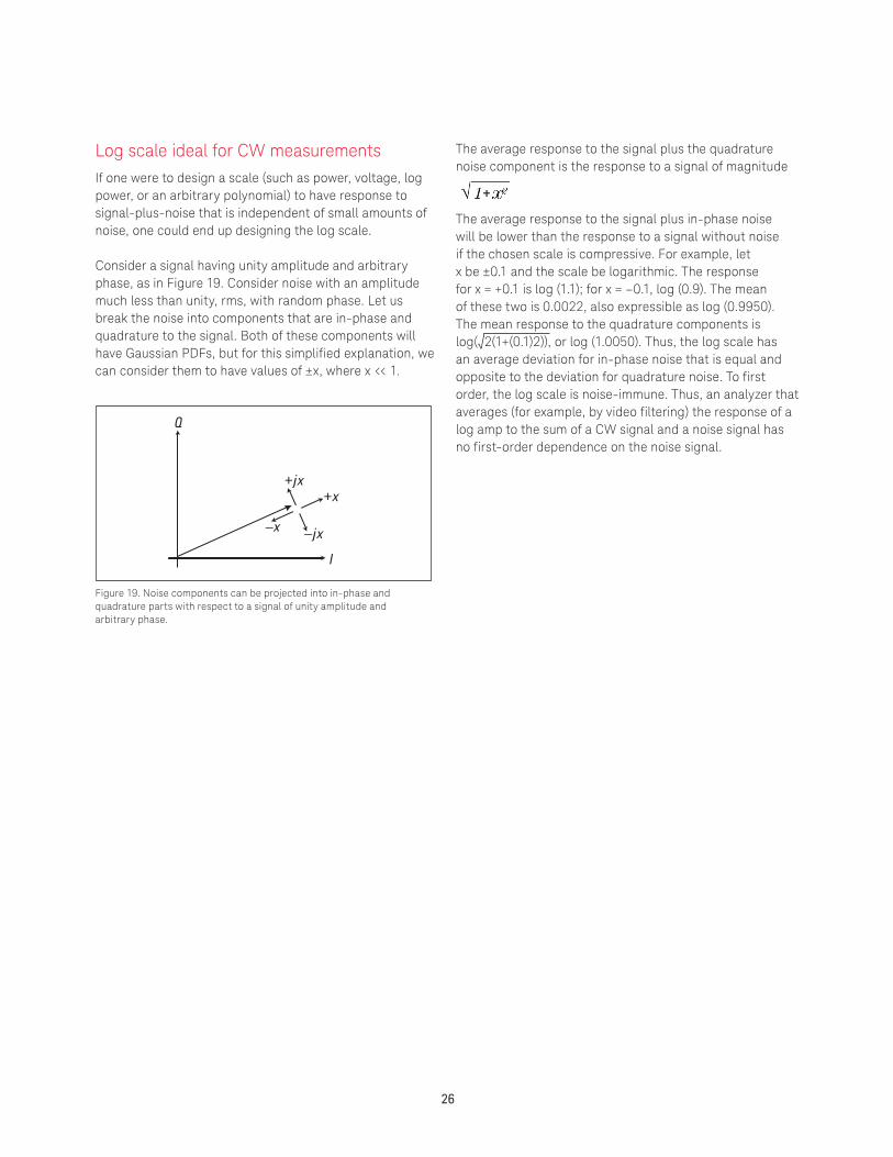
Log scale ideal for CW measurementsIf one were to design a scale (such as power, voltage, log power, or an arbitrary polynomial) to have response to signal-plus-noise that is independent of small amounts of noise, one could end up designing the log scale.
Consider a signal having unity amplitude and arbitrary phase, as in Figure 19. Consider noise with an amplitude much less than unity, rms, with random phase. Let us break the noise into components that are in-phase and quadrature to the signal. Both of these components will have Gaussian PDFs, but for this simplified explanation, we can consider them to have values of ±x, where x << 1.
Figure 19. Noise components can be projected into in-phase and quadrature parts with respect to a signal of unity amplitude and arbitrary phase.
The average response to the signal plus the quadrature noise component is the response to a signal of magnitude
The average response to the signal plus in-phase noise will be lower than the response to a signal without noise if the chosen scale is compressive. For example, let x be ±0.1 and the scale be logarithmic. The response for x = +0.1 is log (1.1); for x = –0.1, log (0.9). The mean of these two is 0.0022, also expressible as log (0.9950). The mean response to the quadrature components is log(√2(1+(0.1)2)), or log (1.0050). Thus, the log scale has an average deviation for in-phase noise that is equal and opposite to the deviation for quadrature noise. To first order, the log scale is noise-immune. Thus, an analyzer that averages (for example, by video filtering) the response of a log amp to the sum of a CW signal and a noise signal has no first-order dependence on the noise signal.
Q
–jx
+x
–x
+jx
I
27
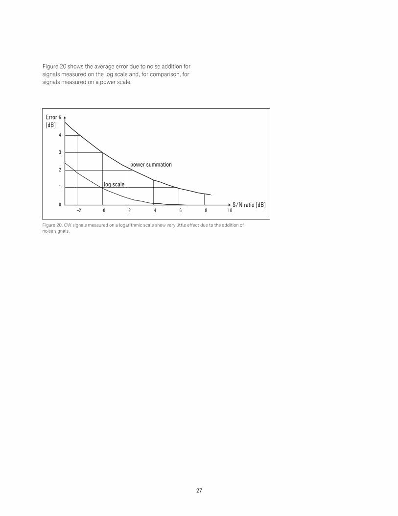
Figure 20 shows the average error due to noise addition for signals measured on the log scale and, for comparison, for signals measured on a power scale.
Figure 20. CW signals measured on a logarithmic scale show very little effect due to the addition of noise signals.
2 0 2 4 6 8 100
1
2
3
4
5Error[dB]
power summation
log scale
S/N ratio [dB]
28
1. Nutting, Larry. Cellular and PCS TDMA Transmitter Testing with a Spectrum Analyzer. Keysight Wireless Symposium, February, 1992.
2. Gorin, Joe. Make Adjacent Channel Power Measure-ments, Microwaves & RF, May 1992, pp 137-143.
3. Cutler, Robert. Power Measurements on Digitally Modulated Signals. Hewlett-Packard Wireless Communications Symposium, 1994.
4. Ballo, David and Gorin, Joe. Adjacent Channel Power Measurements in the Digital Wireless Era, Microwave Journal, July 1994, pp 74-89.
5. Peterson, Blake. Spectrum Analysis Basics. Keysight Application Note 150, literature part number 5952-0292, November 1, 1989.
6. Moulthrop, Andrew A. and Muha, Michael S. Ac-curate Measurement of Signals Close to the Noise Floor on a Spectrum Analyzer, IEEE Transactions on Microwave Theory and Techniques, November 1991, pp. 1182-1885.
7. Gorin, Joe and Zarlingo, Ben. Using Noise Floor Extension in the PXA Signal Analyzer, Keysight Application Note, literature number 5990-5340EN, February 2010.
Bibliography
29
ACP: See Adjacent Channel Power.ACPR: Adjacent Channel Power Ratio. See Adjacent-Channel Power; ACPR is always a ratio, whereas ACP may be an absolute power.Adjacent Channel Power: The power from a modulated communications channel that leaks into an adjacent channel. This leakage is usually specified as a ratio to the power in the main channel, but is sometimes an absolute power.Averaging: A mathematical process to reduce the variation in a measurement by summing the data points from multiple measurements and dividing by the number of points summed.Burst: A signal that has been turned on and off. Typically, the on time is long enough for many communications bits to be transmitted, and the on/off cycle time is short enough that the associated delay is not distracting to telephone users.Carrier Power: The average power in a burst carrier during the time it is on.CDMA: Code Division Multiple Access or a communications standard (such as cdmaOne) that uses CDMA. In CDMA modulation, data bits are xored with a code sequence, increasing their bandwidth. But multiple users can share a carrier when they use different codes, and a receiver can separate them using those codes.Channel Bandwidth: The bandwidth over which power is measured. This is usually the bandwidth in which almost all of the power of a signal is contained.Channel Power: The power contained within a channel bandwidth.Clipping: Limiting a signal such that it never exceeds some threshold.CW: Carrier Wave or Continuous Wave. A sinusoidal signal without modulation.DAC: Digital to Analog Converter.Digital: Signals that can take on only a prescribed list of values, such as 0 and 1.Display detector: That circuit in a spectrum analyzer that converts a continuous-time signal into sampled data points for displaying. The bandwidth of the continuous-time signal often exceeds the sample rate of the display, so display detectors implement rules, such as peak detection, for sampling.Envelope Detector: The circuit that derives an instantaneous estimate of the magnitude (in volts) of the IF (intermediate frequency) signal. The magnitude is often called the envelope.Equivalent Noise Bandwidth: The width of an ideal filter with the same average gain to a white noise signal as the described filter. The ideal filter has the same gain as the maximum gain of the described filter across the equivalent
noise bandwidth, and zero gain outside that bandwidth.Gaussian and Gaussian PDF: A bell-shaped PDF which is typical of complex random processes. It is characterized by its mean (center) and sigma (width).I and Q: In-phase and Quadrature parts of a complex signal. I and Q, like x and y, are rectangular coordinates; alternatively, a complex signal can be described by its magnitude and phase, also known as polar coordinates.Linear scale: The vertical display of a spectrum analyzer in which the y axis is linearly proportional to the voltage envelope of the signal. NADC: North American Dual mode (or Digital) Cellular. A communications system standard, designed for North American use, characterized by TDMA digital modulation.Near-noise Correction: The action of subtracting the measured amount of instrumentation noise power from the total system noise power to calculate that part from the device under test.Noise Bandwidth: See Equivalent Noise Bandwidth.Noise Density: The amount of noise within a defined band-width, usually normalized to 1 Hz.Noise Marker: A feature of spectrum analyzers that allows the user to read out the results in one region of a trace based on the assumption that the signal is noise-like. The marker reads out the noise density that would cause the indicated level.OQPSK: Offset Quadrature-Phase Shift Keying. A digital modulation technique in which symbols (two bits) are represented by one of four phases. In OQPSK, the I and Q transitions are offset by half a symbol period.PDC: Personal Digital Cellular (originally called Japanese Digital Cellular). A cellular radio standard much like NADC, originally designed for use in Japan.
Glossary of Terms
30
PDF: See Probability Density Function.Peak Detect: Measure the highest response within an observation period.PHS: Personal Handy-Phone. A communications standard for cordless phones.Power Detection: A measurement technique in which the response is proportional to the power in the signal, or proportional to the square of the voltage.Power Spectral Density: The power within each unit of frequency, usually normalized to 1 Hz.Probability Density Function: A mathematical function that describes the probability that a variable can take on any particular x-axis value. The PDF is a continuous version of a histogram.Q: See I and Q.Rayleigh: A well-known PDF which is zero at x = 0 and approaches zero as x approaches infinity.RBW filter: The resolution bandwidth filter of a spectrum analyzer. This is the filter whose selectivity determines the analyzer’s ability to resolve (indicate separately) closely spaced signals.Reference Bandwidth: See Specified Bandwidth.RF: Radio Frequency. Frequencies that are used for radio communications.Sigma: The symbol and name for standard deviation.Sinc: A mathematical function. Sinc(x) = (sin(x))/x.Specified Bandwidth: The channel bandwidth specified in a standard measurement technique.Standard Deviation: A measure of the width of the distribution of a random variable.Symbol: A combination of bits (often two) that are transmitted simultaneously.
Symbol Rate: The rate at which symbols are transmitted.Synchronously Tuned Filter: The filter alignment most commonly used in analog spectrum analyzers. A sync-tuned filter has all its poles in the same place. It has an excellent trade off between selectivity and time-domain performance (delay and step-response settling).TDMA: Time Division Multiple Access. A method of sharing a communications carrier by assigning separate time slots to individual users. A channel is defined by a carrier frequency and time slot.TETRA: Trans-European Trunked Radio. A communications system standard.Variance: A measure of the width of a distribution, equal to the square of the standard deviation.VBW Filter: The Video Bandwidth filter, a low-pass filter that smooths the output of the detected IF signal, or the log of that detected signal.Zero Span: A mode of a spectrum analyzer in which the local oscillator does not sweep. Thus, the display represents amplitude versus time, instead of amplitude versus frequency. This is sometimes called fixed-tuned mode.
This information is subject to change without notice.© Keysight Technologies, 2017Published in USA, December 2, 20175966-4008Ewww.keysight.com
31 | Keysight | Spectrum and Signal Analyzer Measurements and Noise – Application Note
www.keysight.com/find/SA
For more information on Keysight Technologies’ products, applications or services, please contact your local Keysight office. The complete list is available at:www.keysight.com/find/contactus
Americas Canada (877) 894 4414Brazil 55 11 3351 7010Mexico 001 800 254 2440United States (800) 829 4444
Asia PacificAustralia 1 800 629 485China 800 810 0189Hong Kong 800 938 693India 1 800 11 2626Japan 0120 (421) 345Korea 080 769 0800Malaysia 1 800 888 848Singapore 1 800 375 8100Taiwan 0800 047 866Other AP Countries (65) 6375 8100
Europe & Middle EastAustria 0800 001122Belgium 0800 58580Finland 0800 523252France 0805 980333Germany 0800 6270999Ireland 1800 832700Israel 1 809 343051Italy 800 599100Luxembourg +32 800 58580Netherlands 0800 0233200Russia 8800 5009286Spain 800 000154Sweden 0200 882255Switzerland 0800 805353
Opt. 1 (DE)Opt. 2 (FR)Opt. 3 (IT)
United Kingdom 0800 0260637
For other unlisted countries:www.keysight.com/find/contactus(BP-9-7-17)
DEKRA CertifiedISO9001 Quality Management System
www.keysight.com/go/qualityKeysight Technologies, Inc.DEKRA Certified ISO 9001:2015Quality Management System
Evolving Since 1939Our unique combination of hardware, software, services, and people can help you reach your next breakthrough. We are unlocking the future of technology. From Hewlett-Packard to Agilent to Keysight.
myKeysightwww.keysight.com/find/mykeysightA personalized view into the information most relevant to you.
http://www.keysight.com/find/emt_product_registrationRegister your products to get up-to-date product information and find warranty information.
Keysight Serviceswww.keysight.com/find/serviceKeysight Services can help from acquisition to renewal across your instrument’s lifecycle. Our comprehensive service offerings—one-stop calibration, repair, asset management, technology refresh, consulting, training and more—helps you improve product quality and lower costs.
Keysight Assurance Planswww.keysight.com/find/AssurancePlansUp to ten years of protection and no budgetary surprises to ensure your instruments are operating to specification, so you can rely on accurate measurements.
Keysight Channel Partnerswww.keysight.com/find/channelpartnersGet the best of both worlds: Keysight’s measurement expertise and product breadth, combined with channel partner convenience.