Keysight Technologies Precision Jitter Analysis Using the Keysight 86100C DCA-J

Application Note

The measurement approach is new and hence a very detailed analysis is provided describing the technique. However, the process of performing a signal quality measurement is extremely simple and in most cases can be performed in a single button press. To begin making measurements immediately, go directly to page 13.

Jitter measurements require an 86100C mainframe with Option 001 trigger hardware and Option 200 jitter analysis software.

Advanced signal analysis in the amplitude domain requires an 86100C mainframe with Option 001 trigger hardware, option 200 jitter analysis software, and Option 300 amplitude analysis/RIN/Q-factor software. Option 300 software must have Option 200 installed to function.

2

Introduction

The extremely wide bandwidth of equivalent-time sampling oscilloscopes makes them the tool of choice for precision analysis of very high-speed waveforms. Historically, low sampling rates have limited their ability to perform in-depth jitter analysis. A revolutionary new sampling/acquisition system in the Keysight Technologies, Inc. 86100C has transformed the sampling oscilloscope into a precision jitter analysis tool. Complete jitter characterization is available including:

– Jitter analysis from 50 Mb/s to over 40 Gb/s – Extremely high sensitivity through low intrinsic jitter (“jitter noise floor”, as low as 200 femtoseconds) – Very simple setup and measurements, typically achieved with a single button press – Separation into random and several deterministic jitter classes – Both histogram and tabular displays of all jitter elements – Jitter analysis linked with precision waveform displays for deeper insight into signal behavior

Signal analysis in the amplitude domain is also available to complement jitter analysis. Mechanisms that cause signal levels to deviate from their ideal amplitude positions can also be separated into random and several deterministic categories. Measurements and displays are similar to those available for jitter analysis.

This product note will review the advanced signal quality measurement capabilities of the 86100C as well as the architectural changes (both hardware and algorithmic) that enable them. A review of the measurement procedures will be presented to allow users to quickly get accurate results. The measurement results will then be reviewed and interpreted. Frequently asked questions and answers are presented.

3

Table of Contents

Introduction .......................................................................... 2

Table of Contents ................................................................. 3

Jitter Analysis Using the Keysight 86100C DCA-J ............. 4

The Case for Jitter Separation ............................................. 4

The 5 Gb/s Measurement Barrier ........................................ 6

Historical Limitations of Legacy Sampling Oscilloscopes for Jitter Analysis....................................... 6

Architectural changes yield fast and accurate measurements ........................................... 8

Deriving a pattern trigger within the oscilloscope ........................................................ 8

Increasing measurement speed through optimized sampling ................................................... 9

Using the New Architecture to Separate Jitter ................. 10

Correlated jitter ........................................................... 10

Uncorrelated jitter ....................................................... 11

Aggregate deterministic jitter (DJ) ............................. 12

Aggregate total jitter (TJ) ........................................... 12

Basic Procedure For Making Jitter Measurements With the 86100C DCA-J ....................... 13

Interpreting Measurement Results .................................... 15

Procedure for Making Amplitude Interference Measurements ........................................... 21

Amplitude Interference Measurement Results .................. 22

Basic Procedure for Making Amplitude Interference Measurements with the 86100C DCA-J ........................ 23

MJSQ: Fibre Channel – Methodologies for Jitter and Signal Quality Specification........................... 24

Understanding the Accuracy of Jitter Measurements Performed with the 86100C DCA-J ............................... 25

Frequently Asked Questions (FAQ’s) .................................. 27

4

Jitter/Amplitude Analysis Using the Keysight 86100C DCA-J

Virtually every high-speed communications design must deal with the issue of jitter. Definitions of jitter as well as its impact on system performance have been well documented but can be generally summarized as follows: When data are misplaced from their expected positions in time, receiver circuits can make mistakes in trying to interpret logic levels. Bit error ratio (BER) is degraded.

As data rates increase, jitter problems tend to be magnified. What might have been considered a small and tolerable time deviation at a lower data rate appears to be large and intolerable at high data rates. Consider that the bit period of a 10 Gb/s signal is only 100 picoseconds. When combined with signal impairments such as at-tenuation, dispersion, and noise, just a few picoseconds of timing instability can mean the difference between achieving or failing to reach BER objectives. The problem is further aggravatedby the difficulty presented in making accurate measurements of jitter. A variety of measurement approaches exist. While the various methods are well thought out and are based upon sound architectures, there has been frustration within the industry around the complexity of setting up a measurement, getting repeatable results, and perhaps more important, getting the various techniques to agree with each other. The measurement problem is severely compounded when the 5 Gb/s data rate threshold is crossed. Above this rate, the list of solutions for jitter measurements is short. The “equivalent time” sampling oscilloscope, with configura-tions having over 80 GHz of bandwidth and extremely low levels of intrinsic jitter, is an obvious candidate for jitter measurements at very high data rates. However, some fundamental limitations of the wide-bandwidth oscillo-scope have historically prevented it from being more than just a coarse jitter measurement tool. These limitations have now been overcome with the new Keysight 86100C DCA-J. Patented architectural changes have resulted in a flexible and easy to use jitter solution based upon a familiar laboratory instrument. Perhaps most important is that this tool provides thorough and accurate jitter analysis at rates from 50 Mb/s to over 40 Gb/s. The combination of highly accurate jitter analysis with the most accurate oscilloscope make this an essential tool for any high-speed digital communications test system.

With the improved hardware of the 86100C, jitter analysis concepts are easily extended into the amplitude domain. This allows an in-depth view into impairments that are related to signal levels, either logic ones or logic zeroes, deviating from their ideal positions.

The Case for Jitter Separation

In many communications systems and standards, specify-ing jitter involves determining how much jitter can be on transmitted signals. Jitter is analyzed from the approach that for a system to operate with very low BER’s (1 error per trillion bits being common), it must be accurately characterized at corresponding levels of precision. This is facilitated through separating the underlying mecha-nisms of jitter into classes that represent root causes. Specifically, jitter is broken apart into its random and deterministic components. The deterministic elements are further broken down into a variety of subclasses. With the constituent elements of jitter identified and quantified, the impact of jitter on BER is more clearly understood. This then leads to straightforward system budget allocations and subsequent device/component specifications.

Breaking jitter into its constituent elements allows a precision measurement of the total jitter on a signal, even to extremely low probabilities. In addition to accuracy, the extensive measurement times often required to assess rare phenomenon can be dramatically reduced. To understand the approach, it is helpful to review the various types of jitter that can exist on a signal.

The first classification is between jitter that is random and that which is not. Jitter that is not random is bounded. That is, its magnitude is finite. In contrast, random jitter is unbounded and within physical limits, can theoretically reach any magnitude. Random jitter (RJ) is often described as having a Gaussian distribution with ‘tails’ that extend indefinitely. Random jitter mechanisms are often due to oscillator phase noise, where the clock used to set data rates cannot produce a pure frequency and exhibits a random deviation from the ideal.

Deterministic jitter (DJ) can be broken into several subclasses. The first division is between that which is correlated to the data sequence or pattern and that which occurs independent of the data. This can be referred to as correlated and uncorrelated DJ. (Note that RJ is also a class of uncorrelated jitter, but is unbounded and not deterministic).

Uncorrelated DJ is most often observed as some form of periodic phase modulation of clocks used to set data rates. This DJ is uncorrelated because its magnitude is indepen-dent of where it is observed in the pattern. Because this jitter is periodic, it is often referred to as periodic jitter or PJ. Uncorrelated jitter can also be due to bounded, but non-periodic sources. Any one-time transient event that causes edge misplacement would be a non-periodic uncorrelated jitter. Its effects would be bounded. This type of jitter is likely not observed, except by coincidence, unless the measurement system were synchronized to the mechanism in some way. For a sampling scope measurement system, this type of jitter would have to systematically repeat to be observed, and would then in effect become a periodic jitter element.

5

Jitter that is correlated to the data pattern can be broken into three categories: Inter-symbol interference (ISI), duty-cycle distortion (DCD), and subrate jitter (SRJ). Measurement of these jitter sources requires each edge in the data pattern be observed.

ISI mechanisms are well known for their impact on digital communications. Reduced or insufficient bandwidth results in reduced edgespeeds. Thus as a transition takes place from a 1 to a 0 or a 0 to a 1, the signal may not reach its intended amplitude before it is required to switch logic levels again. Obviously this will result in vertical eye closure. However, this will also result in both retarded and advanced edges relative to their ideal positions. The level of misplacement is typically a function of the data pattern preceding the edge being observed. (An example of this is discussed on pages 16–19.)

DCD is observed when the durations of logic 1 pulses are different than the duration of logic 0 pulses. It is easily observed in the eye diagram as the nominal eye crossing (where rising edges intersect falling edges) occurring somewhere other than the 50% amplitude point. In that jitter is typically characterized at the 50% amplitude level, rising and falling edges intersecting at a level other than the 50% amplitude implies that edges are misplaced from their ideal positions.

In that ISI and DCD are pattern dependent, they are part of a jitter class called data dependent jitter or DDJ.

Figure 1. Total jitter is composed of several types of jitter Figure 2. Interference is composed of several types of amplitude impairment

SRJ jitter can be viewed as a form of uncorrelated PJ or a form of DDJ, depending upon how it is manifested in the data pattern. Consider a multiplexing scheme where one leg of a data serializer is physically longer than intended. Any bit on this leg is possibly retarded compared to others on different legs. See page 10 for more details on subrate jitter measurements and interpretation.

It is important to reiterate what can be achieved when the various components of jitter can be isolated. Obviously it helps in troubleshooting jitter problems, as the nature/type of the jitter is often a key indicator of the source. A less obvious reason is that it provides a method to accurately assess the aggregate jitter magnitude to very low probabilities without the time required for a direct measurement. The key to the approach is to be able to segregate the RJ from all other sources. This allows a precision assessment of the distribution of the jitter. The extreme jitter magnitudes are effectively the low probability tails due to RJ. Thus determining these values is achieved once the RJ standard deviation is known, in addition to knowing how the deterministic elements interact with the RJ. This is discussed in the remainder of the paper.

For most jitter mechanisms in the time domain, there is a dual mechanism in the amplitude domain. Some excep-tions are that impairments occur at both the one level and the zero level in contrast to jitter which is assessed at the eye-diagram crossing point. Generally, amplitude impair-ment is referred to as “interference”. The aggregate or total interference is the dual to total jitter. Random noise is the dual to random jitter. Deterministic interference is the dual to deterministic jitter. There is no amplitude impair-ment dual to duty cycle distortion, but there is periodic and inter-symbol interference in the amplitude domain.

SRJ

DDJ

DJ

ISI

DCD

PJ

RJ

TJ

DI

ISI

PI

RN

TI

The 5 Gb/s Measurement Barrier

There are a number of well-established tools for jitter analysis. For most, the hardware used to acquire information allows measurements at data rates up to 5 Gb/s and slightly beyond. Thus as systems are being developed requiring transmission rates of 8 and 10 Gb/s, different measurement technologies are required. The wide-bandwidth oscilloscope has a bandwidth in excess of 80 GHz, thus these instruments’ operating ranges are more than sufficient for general waveform analysis to 40 Gb/s and beyond. For the wide-bandwidth oscilloscope, rates that can be measured are dependent on channel bandwidth. Typically, the bandwidth should be at least double the data rate, with bandwidths ranging from 20 to 50, 70 and 80 GHz depending upon the oscilloscope plug-in configuration. As the oscilloscope is DC coupled, low data rates are also within its measurement range.

Historical Limitations of Legacy Sampling Oscilloscopes for Jitter Analysis

Where does the wide-bandwidth sampling oscilloscope fit into the jitter analysis picture? At a first glance, this instrument looks very attractive due to its very low jitter noise floor and the previously mentioned wide bandwidth. Historically, several barriers have existed for efficient and accurate measurements of jitter. Fortunately, the Keysight 86100 DCA has undergone significant architectural changes to overcome these issues. The new Keysight 86100C is referred to as the DCA-J, indicating its function-ality as a digital communications analyzer with extensive jitter analysis capability. The three key historical limitations of equivalent time sampling oscilloscopes, when they are used for jitter analysis are:

– Excessive measurement times due to a relatively slow data acquisition rate

– Requirement of a pattern trigger – Timing measurement errors introduced when – large ranges of timebase delay are used

While the bandwidth of these oscilloscopes is extremely high, the rate at which data is obtained is relatively slow, in contrast with “real-time” oscilloscopes, that have bandwidths > 10 GHz, but which acquire data at rates of up to 40 Gsamples/s. The sampling oscilloscope then has special requirements for the data it can analyze. The signals must be repetitive, as it will take several passes to acquire enough samples to accurately reconstruct a waveform. (An exception to the repetitive signal require-ment is the eye diagram. In this case, samples are acquired at essentially random, but synchronous locations in a bitstream. The common eye diagram is then a composite of samples acquired throughout the stream of data.)

The simplest jitter analysis performed on sampling oscilloscopes consists of projecting a pixel high slice of the eye diagram at the crossing point along the time axis (Fig. 3). This approximates the probability distribution function of the signal’s jitter.

6

The crossing point histogram can be post-processed to provide rudimentary jitter analysis: RJ and DJ can be separated by fitting Gaussian tails to the histogram and TJ can be extrapolated. However, because of the low sampling rate and fluctuations in the histogram population over time, this simple analysis tends to be coarse.

The sampling scope still has the potential to do an accurate jitter measurement. The DDJ can be found by providing a pattern or frame trigger to the oscilloscope. The pattern trigger provides a timing edge that occurs at most once per repetition of the data pattern. Thus, a requirement for the DDJ measurement is a repeating data pattern. RJ, and DJ that is not correlated to the data pattern can be eliminated from the measurement by enabling trace averaging. The location of each edge can be compared to its ideal location through comparison to the clock edge position (if also displayed on the scope) or by comparison of its position relative to the subsequent position measurement of all the other bits in the pattern.

The RJ and uncorrelated PJ can be measured by disabling any trace averaging and measuring a single data edge in the pattern. (Thus the pattern trigger requirement is still in place). Since all the samples are acquired on a single edge, there will be no DDJ component in these data. A data slice at the edge midpoint can be used to generate a time axis histogram that will contain the RJ and uncorrelated PJ. The histogram can then be analyzed and fitted to a curve to determine the critical statistics of these two jitter elements.

While this process is superior to a simple histogram of the eye crossing point in terms of precision and the separating out of the jitter elements, it still has some serious flaws. Perhaps the most important is the amount of time required to acquire a sufficient population for an accurate measurement. Consider that an oscilloscope trace of a data edge is composed of perhaps 100 to 1000 samples. The time between samples is several microseconds (25 microseconds for the Keysight 86100). Thus it can take 25 milliseconds to produce one edge from which a single jitter value can be obtained. Several jitter values are required to obtain sufficient data to produce a significant population from which the RJ and uncorrelated PJ values might be obtained. The time required for this analysis can easily approach several minutes. Amplitude interference analysis is also performed using similar approach, and with similar measurement times.

The situation is more severe when attempting to determine the DDJ, as each edge in the pattern must be analyzed. For an accurate measurement, only a few edges are acquired for any section of the waveform pattern being examined rather than attempting to measure a large number of edges at a reduced resolution. To remove the uncorrelated jitter elements, trace averaging is used. Thus the number of points that must be acquired is multiplied by the averaging factor, perhaps 16. While the time required for a short pattern is manageable and might take a minute or two, patterns such as a 215–1 PRBS (32767 bits) can take many hours to measure.

A second problem with this sampling oscilloscope method is the requirement of a pattern trigger. That is, a trigger coincident with the repetition of the pattern (sometimes also called a frame trigger). While this may be easy to obtain in a test system using an instrumentation pattern generator, many test scenarios will not have this signal readily available. Additionally, the pattern trigger from a pattern generator instrument will typically have some data dependent jitter associated with it. This can corrupt the measurement, particularly when measuring low levels of jitter.

A third limitation associated with legacy equivalent time sampling oscilloscope architectures is a time error that is introduced by using large ranges of timebase delay (required to observe events that occur significant amounts of time after the reference trigger event). In traditional applications of these oscilloscopes, this has not typically been a problem. However, in order to characterize jitter through a pattern (primarily for DDJ), large ranges of timebase delay are typically required. This can introduce significant error into the jitter measurement.

Thus, long test times, the requirement of a pattern trigger, and measurement error from large ranges of timebase delay present significant obstacles for the sampling oscilloscope jitter solution.

7

Figure 3. Jitter observed through the histogram of the eye diagram crossing point

8

Re-timer

High-speed counter(25 to 725 MHz)

Programmable divider(2, 4, 8, 16, 32)

Clock in

50 MHz to 13+ GHz

Count Pulse(1, 2, 3, ..., 223)

Trigger

Figure 4: 86100C conceptual diagram for internally deriving a pattern trigger

Architectural changes yield fast and accurate measurementsTo overcome these historical limitations, fundamental changes to the sampling oscilloscope architecture are required. Once the architecture is improved, the door opens for new measurement algorithms, which can dramatically reduce the time required and significantly improve the accuracy for jitter measurements.

Deriving a pattern trigger within the oscilloscopeA pattern trigger can be derived from a system clock signal. One must know the length of the pattern and the ratio of the data rate to the system clock rate. For example, in the case of the full rate clock, if the pattern length is N, a strobe signal should be generated every time that N clock cycles have been counted. While the concept is very simple, a successful implementation is far from trivial. Consider that any timing imperfections or asynchronism in generating the trigger are manifested directly in jitter measurement error. It is also important for the sampling oscilloscope to have control of the pattern trigger and where it fires in relationship to the pattern. This control enables the oscilloscope to target the sampling at specific locations in the data pattern and to force the data acquisi-tion to be performed over a small range of the timebase. Thus, the internally generated pattern trigger architecture has eliminated both the requirement for a pattern trigger as well as measurement errors induced by large ranges of timebase delay.

With the internally generated and controlled pattern trigger, the oscilloscope can now systematically ‘walk’ through the pattern and determine the nominal location of each edge or signal amplitude in the sequence. When executing this function, averaging is used to remove any uncorrelated jitter/interference mechanisms in order to best determine the average location of each edge/level. The next significant change in this new approach to signal measurement requires a method for dramatically increas-ing the measurement speed.

Figure 5. The edge model yields the amplitude to jitter transfer function

9

Increasing measurement speed through optimized sampling Given that the sampling rates of equivalent time oscil-loscopes are slow, improving the speed of jitter/interference measurements requires that data be collected and processed in a fashion where as many samples as possible contribute directly to the measurement. The main candidate for improvement stems from the fact that, historically, a single jitter/interference value is derived from hundreds of waveform samples. This is because the oscilloscope is fundamentally an amplitude measuring instrument. To determine the position of an edge for a jitter measurement, many samples were required to reconstruct the waveform edge, and from that only a single jitter value was derived.

To improve the jitter measurement efficiency of the oscil-loscope, two important changes are made to how samples are collected. First, rather than collecting samples from all portions of the waveform including where amplitude is somewhat constant (and hence there is no direct jitter information), samples are acquired only from edges. However, this alone would not solve the problem, as many amplitude samples from the edge would still be required to yield a single edge time position and thus a single jitter measurement data point. The key enabler to measurement efficiency is to develop a transfer function that allows the amplitude of any single sample taken from an edge to be directly translated to a jitter measurement value. This is achieved by generating models of the edges.

Consider the edge of figure 5. If the time of the sampling is set up to take place at the 50% amplitude or middle of the ideal, jitter free edge (this is enabled by theinternally generated and controlled pattern trigger), an early arriving signal will have an amplitude above the middle, while a late arriving edge will have an amplitude below the middle level. To determine the amount of jitter on the edge from which the sample was taken, one must know the amplitude versus time shape of the edge. This is effectively an amplitude-to-jitter transfer function - an edge model. Once the edge is modeled, every sample that is taken along the edge yields a jitter measurement.

Two types of edge models are presented - single-edge models and composite-edge models. (The single edge models are used in uncorrelated jitter measurements while the composite edge models are used for data dependent jitter measurements. This is discussed later). A single-edge model is constructed by taking 1024 samples across the entire span of one edge. A mathematical function is constructed that delivers the best fit, in a least squares sense, to the sampled data. A composite-edge model is very similar, except the samples used to construct the model are taken from multiple edges.

A single-edge model is used to describe the amplitude-to-jitter characteristics of a specific edge of a pattern. Composite-edge models are composed of 4096 points and are used to describe the amplitude-to-jitter characteristics of a class of edges. The shape of an edge can be depen-dent upon the preceding bits. The ‘memory’ generally lasts for three or four bits, thus there are several classes or groups of edge shapes possible. A class is defined by two factors - rising versus falling and the preceding bits. For example, ‘00001’ is one class of rising edge, and ‘00101’ is another. Similarly, ‘11110’ is one class of falling edge, and ‘11010’ is another. Consequently, 16 edge classes are defined – 8 rising and 8 falling.

There is some measurement time overhead associated with generating edge models for the several edge classes. However, consider that once the models have been generated, from that point forward almost every sample obtained provides a jitter value. The time required to generate the models is on the order of one or two seconds. This small investment results in orders of magnitude improvement in measurement efficiency. In some recent trials, complete jitter measurements performed on patterns greater than 7600 bits in length were performed in less than 15 seconds. Similar measurements took over 6 hours with the conventional equivalent time sampling oscilloscope.

10

Using the New Architecture to Separate Jitter

The process to determine TJ, RJ and DJ is now described along with the process for determining the subcomponents of DJ - DDJ (ISI, DCD) and PJ.

As described earlier, the oscilloscope will examine the signal to automatically determine the triggering clock rate, bit rate and pattern length (alternatively, the values can be entered manually). Once these values are determined, hardware within the instrument will generate a pattern trigger. The pattern trigger is manipulated to execute the edge modeling process within the pattern. Samples are acquired only on the edges and converted directly to jitter values.

The jitter separation method approaches the task by independently targeting the jitter that is correlated to the data pattern and the jitter that is uncorrelated from the data pattern. The correlated jitter is by definition the DDJ. The uncorrelated jitter is made up of RJ and uncorrelated periodic jitter (PJ).

Correlated jitterAveraging is used to isolate the DDJ. Averaging eliminates the uncorrelated elements. The edge time deviation effects (jitter) that remain are those that are correlated to the data pattern - the DDJ. Composite-edge modeling is used in order to maintain maximum sampling efficiency, as each edge in the pattern must be measured in order to fully characterize the DDJ. The pattern trigger is “walked” through the pattern and samples are taken from every edge. The composite-edge model associated with each edge’s class is used to translate each amplitude measure-ment into a jitter measurement.

The jitter on edges is segregated for the rising edges and the falling edges. A probability distribution function (PDF) histogram is created for both the jitter of the rising edges and the jitter of the falling edges as well as a jitter histogram of all edges. The DDJ is given by the peak-to-peak spread of the histogram of all edges. It is the arrival time difference between the earliest arriving edge and the latest arriving edge. The jitter induced by inter-symbol interference (ISI) is given by the peak-to-peak spread of the rising edges or the falling edges, whichever is greater. Duty cycle distortion (DCD) is given by the difference between the mean of the rising edge positions and the mean of the falling edge positions.

Sub-rate jitter (SRJ) is a term used for jitter which is periodic, correlated to the data, and whose frequency is an integer sub-rate of the data rate. This form of jitter is often associated with multiplexing data structures. For example, if one leg of a parallel data structure systematically results in an edge being late, the jitter will be periodic in nature. If the parallel data structure is eight bits wide, and the length of the data pattern is a multiple of eight, then every eighth bit of the pattern will always be retarded. This would be a form of DDJ. In a similar scenario, if the pattern length is not a multiple of eight, again, every eighth bit will be retarded. However, unlike the pattern which is a multiple of eight in length, as this pattern is repeated the location of the jittered bits within the pattern will con-stantly be changing position. Thus the jitter is not DDJ, but rather uncorrelated PJ. It is correlated to the data stream, but may not be seen systematically on the same bits in a given pattern depending on the relationship between the pattern length and MUX size. Another common source of SRJ is coupling of a sub-rate reference clock onto the full-rate data stream.

Extraction of SRJ is somewhat complex. The fact that SRJ shows up as DDJ when the pattern length is a multiple of any clock divisor used to trigger the oscilloscope is used to segregate the SRJ component and display it as a unique quantity. (It otherwise shows up as PJ). Subrate jitter is correctly reported as a contributor to periodic jitter when it is not correlated to the pattern length, and is correctly reported as a contributor to DDJ when it is correlated to the pattern length. The relative rates of SRJ components will also be reported.

Figure 6. DDJ, RJ/PJ, and TJ histograms with DDJ versus bit - split display

11

Uncorrelated jitterThe approach for determining the uncorrelated jitter (RJ and PJ) takes advantage of the fact that any edge ob-served in isolation will yield uncorrelated jitter information regardless of the pattern dependent elements that effect it. Its deviation about its mean position is dictated solely by the uncorrelated elements. For each data acquisition cycle targeted at uncorrelated jitter, the oscilloscope will acquire all of its samples on a specific edge within the pat-tern, thus all pattern dependent jitter is removed from this data. A single-edge model is used, and samples are taken specifically at the edge. The edge model technique is used to efficiently convert amplitude samples to jitter values. Once a sufficient population is obtained for an edge, subsequent acquisitions are taken from other edges in the pattern, but each individual acquisition record (population) uses data from a single edge. Data from all acquisitions is aggregated into a common histogram.

The internally generated pattern trigger is controlled such that the sampling interval is both precise and consistent sample-to-sample. Thus samples are taken in a highly periodic fashion. This allows the jitter values to be tranformed into the frequency domain using a fast Fourier transform (FFT). This yields the spectrum of the jitter that is uncorrelated with the data pattern, which includes the RJ and uncorrelated PJ. The RJ makes up the noise floor of the spectrum and the PJ shows up as discrete frequency components or line spectra. The RJ is obtained by integrating the noise floor of this spectrum. Prior to the integration, the PJ line spectra are removed, and interpolation is used to fill the ‘gaps’ left behind by the missing lines. The remaining spectrum is due to the random components of jitter. This is integrated to determine the root mean squared (RMS) RJ, that is, the standard deviation of the random jitter distribution.

The line spectra are not used to determine the PJ. The maximum periodic sampling rate of the 86100C is 40 KHz. Any jitter spectral content that is above 20 KHz will be aliased (the frequency of the jitter cannot be determined without additional analysis). This limits the analysis of the jitter spectrum to that of the noise floor described above. The PJ is determined by returning to the accumulated histogram of the jitter values obtained for the targeted edges. This includes the ability to identify the frequencies of the spectra that make up the periodic jitter. Advanced sampling techniques allow accurate identification of periodic jitter amplitudes and frequencies to data rate/4.

A dual-Dirac delta model is used to determine the PJ. The standard deviation of the RJ distribution is given by the measured RMS RJ described above. A dual-Dirac delta model is constructed with two identical Gaussian distribu-tions each defined by the measured RMS RJ value. The separation of the two Gaussian distributions is adjusted in order to match the model to the histogram. The match is made where the peak-to-peak separation representing 99.9% of the area of the model (corresponding to a 10–3 probability) matches the corresponding width containing 99.9% of the area of the measured histogram. (See figure 7.) The PJ value is given by the resultant separation between the means of the two Gaussian distributions. The effective PJ value, independent of the PJ shape is also computed by performing a root-sum-of squares analysis with the standard deviation of the RJ from the RJ/PJ histogram yielding the RMS PJ.

A common question is how valid such an approach is without knowing in advance that the RJ/PJ histogram fits the dual-Dirac model. The RJ, PJ histogram need not have a pure dual Dirac-delta shape in order to be modeled by one. The key intent of the model is to determine the impact of the PJ on the TJ, which in turn must be characterized to extremely low probabilities. In most applications the PJ will typically have a complex distribution that isn’t completely described by any given, well-known model. However, the dual Dirac-delta model is an effective tool to assess and describe the impact of the PJ on the low probability RJ and eventually the TJ. Efficient and accurate evaluation of TJ to low probabilities is one of the fundamental reasons for separating jitter. Interpretation of the PJ magnitudes reported by the 86100C is discussed in more detail in “Interpreting Measurement Results”, page 20.

PJ

RMSRJ

Peak-peak

0.1% ofthe area

0.1% ofthe area

Figure 7. The dual-Dirac delta jitter model

12

Extending the measurement technique to determine the nature of amplitude interferenceTo determine the nature of amplitude interference, whether it is random, periodic, data dependent or a combination of several mechanisms, a similar measurement approach to that used for jitter is used. The oscilloscope timing is configured to take samples in the time center of every bit (the time position is also user definable). Correlated interference is determined by enabling trace averaging and determining the nominal amplitude of each bit. A popula-tion of all the nominal one amplitudes and a population for all the nominal zero amplitudes are collected. The differ-ence between the highest and lowest one levels yields the ISI value for the 1 levels. A similar analysis yields the ISI for the 0 levels.

With averaging disabled, the uncorrelated interference can be determined. Again, the oscilloscope takes samples at the center or user-defined position of the bit period. Data are acquired in a highly periodic fashion. The sample population is converted to the frequency domain. Extrac-tion of periodic interference and random noise is achieved in virtually the same way as uncorrelated jitter. Aggregate deterministic interference is derived similar to aggregate DJ, and aggregate total interference is derived similar to aggregate TJ. Note however, that there are two sets of results: one for logic zeroes and one for logic ones. (For interference analysis, sampling efficiency is achieved by acquiring amplitude samples only in the center of the bit period rather than acquiring the waveform of the entire bit. No edge model is required, as the amplitude results are yielded directly.)

Separating jitter/interference into its constituent com-ponents and then systematically re-combining them to provide an accurate assessment of total jitter/interference is an extensive procedure. However, the measurement process, from the perspective of the user, consists of simply selecting the jitter mode, a single keystroke.

Aggregate deterministic jitter (DJ)The above analysis has resulted in specific values for RJ, PJ, ISI, DCD, SRJ, and DDJ. These contain all the elements of jitter observable with the 86100C. The task now is to accurately combine these elements to produce an aggregate deterministic jitter (DJ) value and finally a total jitter (TJ) value. So far, PDF’s have been determined for the uncorrelated jitter (RJ and PJ) and for the correlated jitter (DDJ). The DJ value is composed of both the DDJ and the PJ, but it is not a simple sum of the values, as each is defined by a unique independent statistical distribution. To determine the aggregate DJ, a method similar to that used to determine the PJ from the RJ,PJ PDF is used. Here the fit is performed at a point where the probability corresponds to 10–3/N, where N is the number of edges in the pattern. The RJ,PJ and DDJ PDF’s are convolved together. The aggregate histogram becomes the total jitter histogram, as it is the PDF of all of the measured jitter - both correlated and uncorrelated - combined in a single histogram. The dual-Dirac delta model method described above for extracting PJ from the RJ,PJ histogram is now applied to the total jitter histogram. Once again, the measured RMS RJ value accurately describes the two Gaussian distributions of the model. The same fitting technique is used, where in this case the model is adjusted to determine the impact of DJ on the total jitter PDF. As the total jitter histogram is the PDF of all jitter elements, the resultant separation of the two Gaussian distributions yields the effective aggregate DJ.

Aggregate total jitter (TJ)The ultimate measure of jitter generation performance of a device under test (DUT) is TJ. The aggregate TJ histogram must then be further analyzed to provide a numerical value that can be used to assess the quality of the DUT. Note that the tails of the aggregate PDF extend indefinitely, so a peak-to-peak value has mean-ing only when associated with a specific probability. A typical approach is to determine the jitter level such that the probability of exceeding it is less than 10–12. The dual-Dirac delta model associated with the total jitter PDF is used to determine this value. TJ is determined by extending the dual-Dirac delta model down to the point where the probability of occurrence is less than one part per trillion of the whole. The width of the model at this threshold is the total jitter. TJ values at other levels of probability are user-definable.

Figure 8. Combined histograms and tabular results

13

Basic Procedure for Making Jitter Measurements with the 86100C DCA-J

The procedure for making a jitter measurement using the 86100C is simple and straightforward.

The signal to be measured is connected to the input channel appropriate for the speed of the signal. As a simple rule, the bandwidth should be at least double that of the data rate. For NRZ signals the fundamental frequency is at half the data rate, so a bandwidth of double the data rate will easily pass the third harmonic of the fundamental frequency. For example, the 54754A, the lowest bandwidth electrical channel for the 86100C has a specified bandwidth of over 18 GHz. Thus it can be used for data rates up to 10 Gb/s (third harmonic being 15 GHz) and slightly beyond. A variety of other plug-ins are avail-able with optical or electrical channels with up to 65 and 80 GHz bandwidths respectively. Channel bandwidths are adjustable. Verify that the channel bandwidth setting is set correctly. Select Setup, Channels, Channel #, Advanced >>, and set the desired bandwidth. The tradeoff for increased bandwidth is increased noise.

The second requirement is to provide a timing reference as a trigger signal. This must be a clock signal at the data rate, or a divided clock. The allowable clock divisors are 2N, 5, 10, 20, and 25. Thus for a 10 Gb/s signal, the allowable clock frequencies are 10 GHz, 5 GHz, 2.5 GHz, 1.25 GHz and so on as well as 2 GHz, 1 GHz, 500 MHz and 400 MHz. Whether full rate or divided, this clock must be synchronous with the data signal. Note that the oscil-loscope sampling process is synchronized by the trigger signal. If the trigger has jitter, the signal under test will be compared to a ‘moving’ reference. This may or may not be desirable. For example, if a recovered clock (a trigger derived from the data signal) is used as a trigger, the jitter that is within the loop bandwidth of the clock recovery system will be present on the trigger. This jitter can be common to both the signal under test as well as the trigger and can be removed from the measurement results. This is a common technique to remove slow, low frequency jitter from the analysis.

Although not required, it is often a good practice to verify that the signal is visible on the instrument display in the form of an eye diagram. This provides a quick check to see that the signal amplitudes and trigger signal are valid

for the instrument. Press the Eye/Mask mode key and the Autoscale key. In one or two seconds, an eye diagram should be visible on the screen. (If very short patterns or large clock divisors are used, a complete eye may not be observed, but the signal amplitudes and triggering can still be confirmed).

Once the signals have been verified, jitter measurements are activated through pressing the Jitter Mode key on the front panel. (Note that the autoscale and Eye/mask steps mentioned above are not required, but are only signal quality verifications. If the signal and trigger are known to be good, the entire measurement setup is achieved by simply pressing the Jitter Mode key).

Figure 9. Pattern Lock trigger setup

Figure 10. Jitter setup menu for customizing the measurement process

14

At this point the instrument will automatically perform all the necessary steps to complete the jitter measurement process. The instrument will not display results for two to three seconds as it collects data to detect the required signal parameters. After this, the jitter results page will appear on the display. This page will display graphical as well as tabular jitter results.

If the pattern length of the input signal is not in the list of pattern lengths to automatically detect, it must be input manually via the Trigger, Pattern Lock Setup dialog (see below). Any pattern length can be added to the auto-detect list by selecting ‘Edit list’ in the pattern length pull-down in the same dialog (see below). For jitter mode operation, the pattern length must be less than 65536 bits. (The instrument can lock to patterns of lengths as high as 223 or 8388607 bits for waveform analysis, but jitter analysis is limited to lengths of 216 or lower).

There is a jitter setup menu available as one of the selec-tions on the left side toolbar in jitter mode. This allows the user to reconfigure a variety of parameters including how data is presented as well as how data is acquired. In most cases, the default state of the instrument is valid, and jitter measurements are performed by selecting the jitter mode key alone.To alter the measurement configuration in Jitter Mode, press Measure, Configure Jitter Measurements, JitterMeasurements.

1 Setup

2 Trigger

3 Pattern Lock Setup for Pattern Length

4 Uncheck Auto Detect

5 Select from list, scroll to bottom, edit pattern

4

1

2 3

5

4

15

In order to interpret the PJ δ-δ value it is important to understand the different impact of different shapes of periodic jitter. Consider the case where the periodic jitter is due to a square wave type signal compared to a triangle wave signal. If the magnitude of the square wave jitter is the same as the magnitude of the triangle jitter, the resulting RJ, PJ population density will not be identical. In the square wave case, the combined RJ PJ distribution can be viewed as the random population being shifted back and forth to the two extremes of the square wave jitter excursion with virtually no ‘dwell time’ between. In the triangle cases, the random population can be viewed as linearly transitioning between the extremes. Clearly the square wave case effectively moves the 10–12 probability events further away from the ideal edge point than does the triangle case. The result is that PJ δ-δ will be larger for a square wave jitter source than for a triangle wave jitter source. This indicates a greater likelihood that the PJ would cause a bit error.

Deterministic jitter (DJ): Similar to periodic jitter, DJ is also expressed with respect to a dual Dirac-delta model. The DJ δ-δ parameter indicates the jitter magnitude required to separate the RJ PDFs to match the dual Dirac-delta model with the TJ histogram population (see Page 15 for a detailed description of the DJ method).

Total jitter (TJ): The TJ value is interpreted as the total effective eye diagram closure in the time axis at a specified BER level (default is 10–12, also a user definable threshold). The closure is expressed in time or unit intervals. The probability that an edge will be misplaced beyond the TJ value is less than the user-defined probability threshold. Thus if the user defined closure threshold is 10–9, and the TJ value provided by the 86100C is 50 ps, the likelihood that an edge will be more than 25 ps late or 25 ps early is less than 1 in 109. If for the same signal the threshold is set to a lower probability, such as 10–12, the reported jitter value will increase significantly, as a much wider population of the distribution function is included in the assessment of TJ. The tabular results include DCD, ISI, DDJ, PJ, RJ, DJ, and TJ.

Interpreting Measurement Results

The methods the 86100C uses to extract the various elements of jitter are described in detail in earlier sections of this paper. Certain jitter components are easy to interpret while others require some further explanation. The following is a brief summary of the measurements and what each is intended to describe.

Intersymbol interference (ISI): This value is determined from measuring the average position of each bit in the pattern with all uncorrelated effects removed. It is the difference between the earliest falling edge and latest falling edge, or the difference between the earliest rising edge and the latest rising edge, whichever is larger.

Duty cycle distortion (DCD): Also determined from the same data set as ISI, this is the difference in the mean position of all falling edges and the mean position of all the rising edges, with uncorrelated effects removed.

Data dependent jitter (DDJ): Also determined from the same data set as ISI, it is the difference in the position of the earliest edge (rising or falling) and the latest edge (rising or falling). Thus the measurement result is dictated by the worst-case bits in the pattern, but does not include the effects of any uncorrelated jitter. Note that as DCD goes to zero, DDJ is equivalent to ISI. As ISI goes to zero, DDJ is equivalent to DCD. DDJ is not necessarily the sum of ISI and DCD. For example, the DDJ can be completely dominated by the ISI component.

Random jitter (RJ): This value quantifies the jitter that is due only to random mechanisms. In that it is Gauss-ian in nature with a magnitude that extends to extreme values (at low probabilities), a root mean square (RMS) value is reported.

Periodic jitter (PJ): This value represents all of the periodic jitter that is uncorrelated from the data pattern. The PJ value is reported in two ways. The PJ δ-δ parameter indicates the jitter magnitude required to separate the RJ PDFs to match the dual Dirac-delta model with the acquired RJ, PJ population (see Page 11 for a detailed de-scription of the PJ method). The PJ value is also expressed as an RMS value in order to help quickly relate to known amounts of injected jitter. For example, if a sine wave jitter source is injected, its RMS value is known, and one should expect the measured RMS value to be very similar to the known injected amount value.

16

DDJ histogram and Composite DDJ histogram: The DDJ histogram is the PDF of the correlated (to the data pattern)jitter including ISI and DCD. The DDJ histogram display shows the DDJ data associated with all of the edges. In the Composite DDJ histogram display the different colors represent the rising edge data, falling edge data, and the composite data for all edges.

Total Jitter histogram: This is the computed histogram derived from all the jitter data. The Total Jitter histogram is constructed by convolving the two directly measured histograms – the RJ, PJ histogram with the DDJ histogram. Note that the 86100C also provides a BERTscan or ‘bathtub’ curve display of the aggregate jitter.

The reported TJ value from the bathtub curve depends on the probability at which TJ is assessed. The default value is at a 1E-12 probability, but this threshold is also user defin-able. The probability threshold is adjusted under Measure/Configure Jitter/Advanced/TJ-TI measurement BER.

Figure 12. DDJ histograms

Figure 13. Total jitter histogram

Figure 14. Bathtub curve for total jitter

Figure 11. RJ, PJ histogram display

Graphical Presentations of JitterOne, two or four graphical displays of jitter are provided depending upon the user-defined configuration (available on the toolbar on the left side of the screen or the jitter setup page of the configure measurements menu). The following graphical displays are available:

RJ, PJ histogram: This is the PDF of random and uncorrelated periodic jitter. The histogram represents all jitter that is not correlated to the data pattern.

17

Composite Jitter histogram: This combines the RJ, PJ, DDJ, and TJ histograms on a common X-axis. In order to provide a single histogram view that provides an overall view of the jitter present in the signal.

All the histogram graphs have no absolute Y-axis scale. The Y-axis magnitude represents the relative population magni-tude for X-axis position, but only for that specific histogram. When several histograms are displayed on a common graph, there is no relative magnitude from graph to graph. This is due to the different histograms being composed of significantly different sample sizes which would typically cause the histogram graphs to have dramatically different sizes and subsequently become difficult to view. Thus when viewing composite displays, the relative spreads are useful to compare, but not the histogram heights.

In some cases, the total number of jitter samples acquired is indicated on the graph.

Figure 16. Composite jitter histogram Figure 17. DDJ versus bit display

Figure 18. Increased resolution for DDJ versus bit

DDJ versus bit: This display shows the data dependent jitter (DDJ) for each edge in the entire pattern. The Y-axis is the jitter magnitude while the X-axis is the relative bit number. The data is plotted on top of an ideal representation of the data pattern. This enables quick reference of DDJ data to its position in the pattern. In order to optimize data visualiza-tion, the ideal data pattern background is not shown when the screen space-to-data ratio is less than 2 pixels per bit.

It is also possible to adjust the span of the DDJ versus bit display. Using a mouse or the touchscreen, a box can be created by clicking (or touching) and dragging. The box width will set the new span of the graph. Also, the oscil-loscope’s horizontal span and position knobs are reassigned in Jitter Mode to control the span and position of the DDJ versus bit display. If the span of the DDJ vs. Bit includes the earliest or latest edge of the pattern (noted with a blue or red dot respectively), selecting (mouse or touchscreen) the [Earliest Edge] or [Latest Edge] screen labels will position that edge at the center of the screen.

Figure 15. Setup for total jitter bathtub

18

The ability to find the worst-case bits for DDJ leads to important jitter analysis techniques unique to the 86100C. Recall that the native measurement capability of the instrument is as an oscilloscope. Thus it is a simple process to examine the waveforms of identified bits with the oscilloscope. This data can easily be assessed with respect to the input signal, as the actual waveform can be precisely viewed by switching to oscilloscope mode. The relative trigger bit can be adjusted in order to view specific sections of the pattern. While the 86100C has locked on to the pattern (using Pattern Lock triggering), the trigger level adjustment knob is reassigned to control the relative bit position of the oscilloscope’s trigger in the pattern. The relative trigger bit can also be set directly to a given value in the Trigger Setup dialog.

Consider the DDJ versus bit display of figure 20. The latest edge is indicated by the red dot, the earliest by the blue dot.

The resolution of the DDJ versus bit display is increased (either by clicking and zooming in, or using the timebase span and delay knobs) to focus in on the latest edge as seen in figure 21.

Pressing the [Latest Edge] label will position the graph so that this bit is at center screen. Note that this is position 680 for the current pattern lock configuration. (Remember, the pattern lock 0 bit position is uniquely determined each time the jitter mode is activated, a pattern lock is executed, or an autoscale is performed while in jitter mode. Thus the numerical position assignment for any specific bit in a pattern may change from setup to setup.)

At this higher resolution setting, the logical pattern is shown in addition to the time deviation for each edge. From this, one can conclude that the worst-case deviation position occurs at the end of a long run of logical 1’s. It may be useful to now examine the actual waveform of this bit sequence. Again, this is found at trigger bit position 680. The trigger bit location, and what the 680 value represents, is best understood by examining how samples are taken for the jitter measurements. This can be viewed by raising up the graphical panel, achieved by selecting the ‘Graphs’ label located on the lower right area of the DDJ versus bit panel (also just above the ‘Div Ratio’ label of the jitter numerical results panel). When this is selected, the graphical panel is raised to display the eye diagram of figure 22.

Figure 20. Troubleshooting DDJ

Figure 21. Worst case DDJ

Figure 19. Zooming in on the DDJ versus bit display

LatestEarliest

Latest

Bit #

Long sequence of 1’s

19

This display shows the actual time or display position where the edge samples are being acquired (the right side crossing point). This also represents where on the oscil-loscope timebase a specific edge number will be located when the trigger bit is adjusted to a specific value. This can be seen by going to oscilloscope mode, selecting the “Trig Bit” display button (lower right area of the display), and changing the trigger bit to a value of 680. Note that when going to oscilloscope mode from jitter mode, the pattern lock settings are maintained. Thus even though a clock signal is triggering the oscilloscope, the signal will be observed as if a pattern trigger were being supplied to the oscilloscope. See figure 23.

With a wider view of the pattern, the specific waveform behavior leading up to the latest edge can be observed. In this case, an ISI type problem causes the trajectory of a 1 to a 0 to start at a relatively high amplitude when preceded by several consecutive 1’s. Starting from this higher amplitude, a longer time is required to reach the edge threshold, resulting in the effective edge delay.

As was observed in the DDJ versus bit display, the latest edge occurs after a run of logical 1’s and is confirmed with the waveform above. The timebase of the oscilloscope can be adjusted to get a broader view of the pattern. Note that the delay adjustment knobs shift the waveform position, and will alter the relationship between the trigger bit number and its screen position. Before changing the timebase span, a good practice is to place a marker on the bit edge so as to not lose track of the specific edge being examined. Timebase adjustments are achieved as in conventional oscilloscope usage, through the time span and delay controls or knobs. Note that once outside of jitter mode, the trigger level knob and the time span (and delay if required) controls are returned to their normal operational modes.

Figure 22. Time position of triggered bit

Figure 23. Worst case Late edge view

Figure 24. Worst case Late edge within pattern

20

In a similar analysis, the earliest edge can be zoomed in on in the DDJ versus bit display and determined to be at edge position 243. Going to oscilloscope mode and setting the trigger bit to position 243, the earliest edge can now be observed. See figure 25.

A marker is placed on the edge and the time span is increased to observe the patterns leading to the earliest edge, as seen in figure 26.

In this case, the root cause is again due to an ISI effect, but the result is essentially the opposite of the latest edge and is observed at the center of the display. After a long run of 1’s, the transition from a 1 to a 0 is retarded. The transition to the 0 level never reaches down to its intended amplitude before a transition back to a 1 begins. Thus the transition begins from a much higher amplitude than intended and the threshold level is crossed earlier than any other edge.

To observe the overall waveform and the relative edge positions of the entire pattern, the eye diagram display is used. The instrument can be switched to eye/mask mode. Again, the pattern lock configuration produced in jitter mode is maintained. Thus an effective pattern trigger is synchronizing the sampling process. Rather than display-ing a pattern sequence as in oscilloscope mode, an eye diagram is displayed. However, rather than the common eye diagram, this eye diagram is produced one continuous trajectory at a time. This is referred to as eyeline mode. The eyeline view shows the earliest and latest edges, as well as those in between. (As DDJ is reduced, or the pattern length is increased, the displayed edges tend to blend together.) The default condition for eyeline mode employs trace averaging to allow clearer viewing of the individual traces with uncorrelated impairments such as RJ, PJ, and noise removed. See figure 27. Note the Trig/Bit button shows the ‘eye’ symbol, indicating eyeline operation.

Figure 26. Worst case Early edge within pattern

Figure 25. Worst case Early edge

Figure 27. Eyeline view of eye diagram

Eyeline mode indicator

21

Isolating individual periodic jitter elementsPeriodic jitter can be either correlated or uncorrelated to the data rate of the signal being observed. Jitter that is at rates that are integer divisors of the data rate is referred to as subrate jitter (SRJ). Jitter that is at a rate that is not an integer divisor of the data rate is referred to as periodic jitter. The 86100C has the ability to isolate either periodic or subrate jitter signals and display them as individual entities. When in jitter mode, selecting the “Frequency” tab on the left side of the instrument screen enables the jitter frequency measurements. Selecting the PJ frequency results tab will allow the display of both subrate and periodic components.

The RMS value of subrate jitter frequencies are available for data signals at datarate/128 to datarate/4. When clocks are measured the upper limit is clockrate/2. The three largest (in magnitude) components are displayed. Asynchronous periodic jitter is derived from the FFT spectrum of uncor-related jitter that is also used to determine RJ. Pressing the “Resolve” button allows the individual periodic jitter frequencies and magnitudes to be determined. Although the sample rate of the 86100C is slow, automatic adjust-ment of the sample rate allows frequencies well beyond the sample rate to be uniquely identified. The allowable frequency range that can be isolated is from under 100 Hz to datarate/4.

Periodic jitter is often due to complex waveforms rather than simple sinusoids. Selecting the PJ waveform button allows the overall periodic jitter waveform to be observed, typically composed of a fundamental and harmonic tones. For example, if spread spectrum clocking is used, the periodic jitter waveform can be observed as a triangle signal.

Procedure for Making Amplitude Interference Measurements

In the default configuration, only jitter measurements are made when the Jitter Mode key is pressed. Amplitude interfer-ence results are obtained by either selecting the amplitude tab (left side of the screen), or, while in Jitter Mode selecting the Setup and Info button (lower right screen), Config Meas, Amplitude Meas and checking the “perform Am-plitude Meas box, or selecting Measure/Config Jitter Meas/ Amplitude/ and checking the “Perform Amplitude Meas” box. Note that there is a small penalty in measurement time to have both jitter and amplitude measurements available compared to jitter measurements alone. Thus the amplitude analysis should be deactivated when measurement time is important and only jitter results are required.

Similar to jitter analysis, amplitude analysis yields total interference (TI), random noise (RN), deterministic interfer-ence (DI), inter-symbol interference (ISI), and periodic interference (PI, rms and δ-δ). There is flexibility in how the interference measurements are setup. Press Measure/Config Jitter Meas/Amplitude.

Measurement location: Nominally at 50%, this determines the point in time within a bit period where the amplitude analysis will take place on the one and zero levels of the signal

Ones, zeroes, or both: “Graph level setting” determines which logic levels will be included in the interference analysis. The analysis can be for only one levels, only zero levels, or both (the default condition).

Units: The interference values can displayed in absolute units of Volts or Watts, or as a percentage of a unit amplitude (UA). Unit amplitude is analogous to the time unit interval (UI), where one UA is the difference between the nominal one level and the nominal zero level.

Figure 29: Setup page for amplitude interference measurements

Figure 28: Isolating periodic jitter components

22

One/Zero level definition: Interference analysis results can be displayed relative to a Unit Amplitude. What defines a unit amplitude (UA) can be controlled by the user. UA can be limited to special data pattern cases. For example, it can be desirable to define UA using bits that are not influenced by the transition from the opposite logic level. If the instrument is placed in Minimum Consecutive Identical Digits (CID) mode, the instrument can be configured to define UA using only bits that have been preceded by a specific number of similar bits and followed by a specific number of similar bits. For example, if Minimum Leading CID is set to 3 and Minimum Lagging CID is set to 2, the only ones that will contribute to the UA value are those that have been preceded by at least 3 ones and are followed by at least 2 ones (with a similar segregation for zeroes). If Average One/Zero Level is selected, all bits will contribute to the computation of UA

Amplitude Interference Measurement Results

The results obtained from the amplitude analysis are analogous to the time domain jitter results. In general, the instrument works essentially the same way for inference analysis as it does for jitter analysis. The advanced trigger-ing techniques allow each bit to be examined to determine correlated effects, as well as make multiple measurements on individual bits to determine uncorrelated effects. Frequency domain analysis through FFT’s is used to extract random components. Dual-Dirac modeling techniques are also carried from the jitter domain and used in the interference domain. The details of these approaches are not repeated here.

As in the jitter domain, the key to making an accurate assessment of the aggregate or total interference is to separate out the individual components of the amplitude fluctuation and build a model that allows an accurate assessment of the total. The various elements of interference are related as follows: Data dependent (Correlated) Interference: In the amplitude domain,

interference that is correlated to the data pattern is observed as Inter-symbol Interference (ISI). With averaging applied to remove uncorrelated interference, the nominal amplitude of each bit in the pattern is determined. ISI for logic ones will be the difference between the highest one level of the entire pattern and the lowest one level of the entire pattern. ISI for logic zeroes will be the difference between the highest zero level and the lowest zero level (also over the entire pattern).

Uncorrelated Interference: There are two types of interference that are measured and are uncorrelated to the data pattern. One is Periodic Interference (PI) and the other is Random Noise (RN). Random noise is unbounded (within the physical limits of the system). It is determined by collecting a population of samples on a given bit in a highly periodic fashion. The population is converted to the frequency domain and the random component is extracted. Periodic elements are also derived from a single bit (See uncorrelated jitter on page 11). Individual results are obtained for both logic ones and also for logic zeroes.

The total Deterministic Interference is obtained through combining the periodic and inter-symbol interference. Total Interference is obtained by combining the deterministic interference and the random noise. (See page 12).

Figure 30: Total interference is composed of several types of interference

23

Basic Procedure for Making Amplitude Interference Measure-ments with the 86100C DCA-J

Once the instrument has been configured as described above, the procedure for making the measurements is identical to that used for making jitter measurements. For the vast majority of cases requires the user simply presses the jitter mode button.

Interpreting amplitude measurement resultsThe definitions for the various interference parameters parallel those in the jitter domain (see page 15)

Inter-symbol Interference (ISI): ISI for logic ones will be the difference between the highest one level of the entire pattern and the lowest one level of the entire pattern. ISI for logic zeroes will be the difference between the highest zero level and the lowest zero level (also over the entire pattern)

Random Noise (RN): This value quantifies the interference that is due only to random mechanisms. In that it has a Gaussian distribution, it is reported as a root mean square (RMS) value.

Periodic Interference (PI): This represents all uncorrelated interference that is not measured as random interference. It is considered to have bounded distributions. It is reported as both an RMS and PI δ-δ value (derived from a dual-Dirac model of the total uncorrelated interference, which includes both the periodic and random interference).

Deterministic Interference (DI): This is reported as a DI δ-δ value and is derived from the TI histogram population, analogous to deterministic jitter (see page 15). It represents the effect that all deterministic interference has on the overall vertical eye closure exclusive of the random interference.

Total Interference (TI): The TI value is interpreted as the total effective eye closure in the amplitude axis at a specified BER level (default at 10–12, but also user definable). The likelihood that a bit level will exceed the TI level is given by the TI BER threshold.

Signal Amplitude: This is the difference between the nominal one and nominal zero level. Note that the bits used for this analysis are those configured in the “One/Zero Definition” as part of the Amplitude Analysis setup. This value also is used to define one amplitude unit or UA.

Eye Opening: This is the height or vertical opening of the eye in the amplitude axis at the TI threshold. It is effectively the height of the amplitude bathtub curve. The probability that a bit level will fall within the region of the eye height opening is less than the TI threshold level.

Q: This represents the signal to noise ratio of the eye diagram. It is given by:

Mean 1 level - Mean 0 level ————— 1 level noise + 0 level noise

Where the mean signal levels are defined by the “One/Zero Definition” in the setup menu and the noise values are the RMS RN values for the one and zero values. BER for a noise limited system can be estimated from Q.

Combining jitter and amplitude resultsPerforming both jitter and amplitude analysis provides important insight into whether a signal BER performance is limited by timing problems or interference problems. Two additional parameters are provided:

BER Floor: This is a measure of the best BER performance that can be achieved for the measured signal, due to either amplitude or timing closure of the eye. It is the BER level at which the sides of the bathtub curve (either jitter or amplitude) intersect. The value displayed will be the worst of the two results. If the intersection occurs at an estimated value that is lower than 10–18, the value is listed as being less than 10–18 without attempting to report what the actual value is.

BER Limit: The domain in which the worst case eye closure occurs, either jitter or amplitude, is listed. If the eye closure in both domains is similar (the ratio of the two estimated BERs is within a factor of two), the signal will be noted as being “balanced”.

24

MJSQ: Methodologies for Jitter and Signal Quality Specification

The 86100C is capable of performing measurements according to the T11 Fibre Channel MJSQ standard . Within the standard document this type of measurement capability is generically referred to as the “enhanced equivalent time sampling oscilloscope”. The MJSQ technique specifies instruments produce the cumulative distribution function (CDF) of the aggregate jitter, and from this a generic formula is used to extract RJ and DJ, independent of what type of instrument is used to collect the jitter data. The 86100C will produce the CDF for this purpose. In that the jitter separation techniques used within the 86100C have been optimized specifically for a sampling oscilloscope architecture, there may be some cases where the RJ and DJ values provided automatically by the instrument may vary to some degree from those derived from the CDF and post processed by the generic MJSQ algorithm. See “Understanding the accuracy of jitter measurements performed with the 86100C DCA-J” on page 25.

Measurement requirements and limitations of the DCA-J in jitter modeThe basic requirements for the 86100C to perform jitter and interference measurements are specific to the signal used to trigger the instrument and the data sequence of the signal being measured. The trigger signal must be synchronous to the data. If there is no trigger signal, the measurement cannot be made. Allowable divide ratios (the ratio of the data bit rate to the trigger clock rate) are 1, 5, 10, 15, 20, 25, 30, 35, 40, 45, 50, 66, 100, and 2N, where N is an integer between 1 and 7. If no clock is available, a clock recovery system such as the 83496 Series of plug-in modules, can be used to provide a clock.

The data pattern must be continuously repeating, with no idle states. The pattern length must not exceed 216 (65538 bits) while operating in Jitter Mode. The instrument will au-tomatically determine the pattern length if it is available in its lookup table. The lookup table includes 2N and 2N–1 for N=1 through 23, as well as the common jitter test patterns (K28.5,CJPAT, CRPAT, SCPAT, JTPAT, SPAT). Other pattern lengths can be added to the lookup table. Once added, the instrument will then be able to automatically detect and lock to that sequence. Note that while Jitter mode allows pattern lengths up to 216, Pattern Lock can function for pattern lengths up to 223 in Oscillscope or Eye/Mask modes (The lookup table can be edited by selecting the “Pattern Lock Setup” tab of the trigger setup dialog, pressing the “Select From List” button next to the Pattern Length, and choosing “Edit List” from the displayed selections.)

The instrument itself will contribute to the jitter. However, this can be as low as 800 femtoseconds in a standard 86100 configuration and below 200 femtoseconds when using the 86107A precision timebase module. Thus the effective jitter noise floor or measurement sensitivity level is extremely low, making the 86100C one of the most sensitive jitter analysis tools available.

As the jitter values are obtained through the edge model transfer function, this places some limits on the magnitudes of jitter that can be measured. As edge speeds become very fast relative to the bit period, the magnitude of jitter that can be accurately measured is reduced. The risetime or falltime of the signal should exceed the sum of the peak-to-peak PJ and double the RMS RJ. The DDJ magnitude is not restricted by the edgespeed provided the edgespeed exceeds the peak PJ and double the RMS RJ. A good guideline for the allowable measurement range is:

Risetime or Falltime > (2 RJ rms + PJ pp)

25

Thus the RJ and PJ jitter magnitudes that can be observed must be less than half of a bit period. Another quick ‘rule of thumb’ analysis for allowable jitter and edge speed is to observe the eye diagram display. Typically, if there is an open region between the crossing point and the 1 rail or the 0 rail, jitter measurements can be made.

Figure 31: Allowable jitter (PJ, RJ)

It is interesting that large amounts of ISI tend to increase the levels of RJ and PJ that can be observed. This is because the ISI mechanisms tend to increase rise and falltimes. Thus as impaired signals are constructed for receiver stress testing, larger values of RJ and PJ can be observed after ISI jitter is included, but not before.

An essential aspect of an instrument’s ability to provide accurate measurements is its ability to recognize when the results are questionable. Rather than generating erroneous results, the 86100C will indicate suspect measurement con-ditions to the user, or in some cases abort the measurement process. If the data rate or pattern length changes, the 86100C will no longer be locked to the signal and be able to make accurate jitter measurements. When this occurs, the instrument will halt measurements and indicate that the synchronization to the pattern has been lost. Instructions to re-acquire the pattern are presented.

If the synchronization to the pattern is stable, but the signal quality is such that the measurement process is incapable of providing good results, the instrument will flag the results with question marks. This may occur when the jitter magnitude exceeds the allowable measurement range based upon the edge model.

Understanding the Accuracy of Jitter Measurements Performed with the 86100C DCA-J

Although the 86100C should provide accurate jitter measurements based upon its wide bandwidth and low intrinsic RJ and DJ, the measurement technique must still be proven. A common technique to verify measurement accuracy is to make comparisons to TJ measurements made with a BERT. The BERT measurements are performed directly to low probability levels without any extrapolation. While this comparison technique provides some level of measurement confidence, it is not ideal. It is not traceable to internationally recognized standards. A more valid approach is to have a jitter signal source with known values of jitter. This is not a trivial engineering problem, as jitter can be comprised of many different signal types. Thus the ideal jitter source must be capable of simultaneously producing several types of jitter, each with adjustable magnitudes, and for PJ, the shape of the jitter should also be adjustable. Again, this must all be done in such a way that the jitter of the signal is known with a high degree of accuracy, and ideally the values are traceable.

To verify the performance of the 86100C DCA-J, a transmitter with adjustable jitter, traceable to NIST, was constructed. The verification of its jitter was performed as follows:

PJ is verified through spectral analysis and a Bessel null technique providing jitter levels known within 1%. Range of adjustment in the trial: ~0 to 0.068 UIRMS

ISI is produced using various lengths of copper traces on common backplane material. ISI quantities are determined through S-parameter analysis using precision network analyzers. ISI values are known to 1%. Range of adjustment in the trial:

~0 to 140 ps

DCD is provided through an adjustable pattern generator and verified through oscilloscope amplitude measurement. DCD values are known to 1%. Range of adjustment in the trial:

~0 to 14 ps

RJ is produced through an arbitrary waveform generator using random number generators. Number lengths allow statistical variation to below 1 in a trillion values, thus providing truly random jitter beyond the typical 10–12 total jitter values generally measured. RJ values are known to < 1.5%. Range of adjustment in the trial:

0.685 to 5.62 psRMS

Open region

26

The verification of 86100C measurement accuracy is performed by subjecting it to a large variety of jitter combinations. Specifically, RJ, ISI, DCD, and PJ are systematically adjusted to low, medium, and high levels (as well as ‘off’). In addition, PJ waveform types are also adjusted. Thus an extensive matrix of jitter conditions are presented to the instrument under test. For example, one signal configuration would be to have high RJ, low ISI, no DCD, and medium amplitude triangle wave PJ. Another configuration might be to have low RJ, high ISI, medium DCD, and large sinusoidal PJ. Again, the validity of the analysis is based upon the jitter being of known quantities as well as being adjustable. In addition to testing the accuracy of the 86100C, the trial also included the common measurement tools found in the MJSQ document (real-time oscilloscopes, time interval analyzers, and BERTs).

Several amplitude levels for several types of jitter resulted in 37 unique test conditions. The data set is significantly large. However, the following conclusions were quickly apparent. Within its designed range of operation there is currently no instrument available that is more accurate than the 86100C for making jitter measurements. This can be shown with results from two of the most difficult measurements: RJ assessments in the presence of other jitter elements, and accurate TJ measurements over a wide range of jitter conditions. The results for all measurement tools are displayed relative to the known values. The measurement error is displayed in picoseconds for each

of the 37 test configurations. Results from the three other instrument types are also included, but are intentionally not individually identified. The data rate was 2.5 Gb/s with a 127 bit PRBS pattern.

ResultsThe results for the 86100C exceed expectations, but in retrospect should not be surprising. Given the low intrinsic RJ and DJ of the instrument and its very wide bandwidth, critical sources of measurement error are reduced to small levels. At the time of the trial, use of the 86107 precision timebase had not been enabled. The small measurement errors in the 86100C are likely to be reduced to negligible levels, particularly for the measurement of RJ with the 86107 in the measurement system. A complete report on the measurement experiment can be found at http://literature.cdn.keysight.com/litweb/pdf/5989-3205EN.pdf. The 86100C results in almost every case actually fell within the range of uncertainty to which the actual jitter values were known. Thus the actual measure-ment errors may be smaller than indicated in the results tables. It is important to realize that the instrument with the highest accuracy is also the least expensive, the easiest to use, and has the widest data rate range in addition to its ability to operate as a high performance oscilloscope.

Jitter Conditons (1-37)

Erro

r (ps

)

60

50

40

30

20

10

00 10 20 30

TJ @ 1E-12

MJSQ 1

MJSQ 2

MJSQ 3

86100C

Figure 33. Error in measured TJ versus DCD/ISI/PJ/RJ condition

Jitter Conditons (1-37)

Erro

r (ps

)

4.00

3.50

3.00

2.50

2.00

1.50

1.00

0.50

0.000 10 20 30

MJSQ 1

MJSQ 2

MJSQ 3

86100C

Figure 32. Error in measured RJ versus DCD/ISI/PJ/RJ condition

27

Q: What happens when the RJ PJ histogram is not a Dual Dirac?A: The RJ, PJ histogram need not have a pure dual Dirac-delta shape in order to be modeled by one. The key intent of the model is to determine the impact of the periodic jitter at very low bit error ratio (BER) levels. In most applications the PJ will typically have a complex distribution that isn’t completely described by any given, well known model. However, the dual Dirac-delta model is a great tool to assess and describe the impact of the PJ on the low probability jitter.

Q: Why do the jitter measurements from Eye Mask Mode (Jitter ρ-ρ and Jitter RMS) differ from the results obtained in Jitter Mode?A: The Jitter ρ-ρ measurement of Eye Mask Mode is simply the time difference between the earliest waveform sample and latest waveform sample from a vertically thin histogram at the eye diagram crossing point. Jitter RMS from Eye Mask Mode is simply the standard deviation of that histogram. (This histogram is composed of all jitter elements present).

In Jitter Mode, jitter components are distinctly identified. Random jitter is presented as an RMS value. This represents the standard deviation of the random jitter. (This is in contrast to the Jitter RMS value of Eye Mask Mode, which includes all jitter components). Total jitter from Jitter Mode is derived from all jitter components. However, unlike Jitter ρ-ρ from Eye Mask Mode, Total Jitter is extrapolated to very low probabilities (10–12 typically). In theory, if samples were collected for many hours, Eye Mask Mode Jitter ρ-ρ would converge to a value similar to Total Jitter. Total Jitter from Jitter Mode should be used as the precision measurement for all components of jitter combined.

Q: Can I Use the 86107 precision timebase module with the 86100C? Will it improve jitter mode measurements?A: The 86107 precision timebase can be used with the 86100C in every application it was used for with the 86100 A and B mainframes, such as eye diagram analysis on ultra high-speed data rate signals or signals with extremely low jitter. No special options are required. The 86107 can also be used with the 86100C in jitter mode to reduce the jitter measurement floor below 200 femtoseconds.

Frequently Asked Questions (FAQ’s)

Q:Is this functionality available on an 86100A or 86100B?

A: No. This functionality is only available on the 86100C. There is significantly different hardware in the 86100C as compared to the 86100A and B, so it’s only available on the C. But all of the modules that you own for an 86100A or B will work in the 86100C.

Q: What instrument options are required to perform jitter measurements?A: Option 001 (mainframe pattern lock hardware) and Option 200 are required.

Q: What instrument options are required to perform amplitude interference measurements?A: Option 001 (mainframe pattern lock hardware), Option 200 Advanced Jitter Analysis software, and Option 300 Amplitude Analysis/RIN/Q-factor software.

Q: How long does it take to measure all the jitter components?A: It does depend on the pattern length. For very short patterns such as a PRBS-7, it’s just a few seconds. In the case of a PRBS-15 pattern, it’s on the order of about 45 seconds to a minute, depending on the amount and makeup of the jitter. Typically on the order of a minute for a PRBS-15.

Q: Is all the uncorrelated data collected from the same edge or bit?A: Technically the uncorrelated results should not really depend on which edge or bit the data came from. In theory you should be able to collect all the necessary data from a single edge or bit. In practice, as data is continually acquired the instrument will collect data from several edges and bits and combine the results.

Q: Are you able to do bathtub curves?A: Yes. BERTscan displays, commonly known as bathtub curves are available with 86100C Options 200 and 300.

Q: Have you done any correlation data using your BERT instruments?A: Rather than simply compare results to a BERT, we have constructed a jitter source with known jitter parameters. This then allows us to know what the ‘right’ answer is rather than comparing it to another measurement. The 86100C performs with the highest precision within its allowable measurement range.

28

Q: How many edge transfer function models do you have?A: There can be up to as many single-edge models as there are edges in the pattern, and there are 16 composite-edge models. Two types of edge models are used: single-edge models and composite-edge models. A single-edge model is constructed by taking samples across the entire span of one edge. A composite-edge model is very similar, except the samples used to construct the model are taken from multiple edges. A single-edge model is used to describe the amplitude-to-jitter characteristics of a specific edge of a pattern. Composite-edge models are used to describe the amplitude-to-jitter characteristics of a class of edges. A class is defined by two factors - rising versus falling and the four preceding bits. For example, ‘00001’ is one class of rising edge, and ‘00101’ is another. Similarly, ‘11110’ is one class of falling edge, and ‘11010’ is another. Consequently, 16 edge classes are defined - 8 rising and 8 falling.

Q: Why doesn’t your PJ, DCD, and ISI add up to the total DJ?A: While PJ, DDJ, ISI, and DCD are all forms of deterministic jitter, DJ is not a simple arithmetic sum of these constituent components. Rather, the DJ distribution is a result of the convolution of the constituent distributions. The DJ value that is combined impact of all of the constituent components at low bit error ratio (BER).

Q: What causes the 86100C to not be able to lock on to a pattern and perform jitter measurements?A: There are a few possibilities for not being able to lock to a pattern. If the pattern length is not one in the instruments lookup table, it will not lock to it. This is solved by simply editing the table to include the new pattern length. (Note, the length, and not the pattern need to be entered). Another possibility is that the data pattern is not stable. That is, one or more of the bits in the pattern are changing states. This can be verified through overriding the pattern autodetect feature (see page 14) and forcing the pattern length to the expected value. A pattern trigger will be generated at this pattern length, whether the pattern is this length or not. The waveform can then be viewed in oscilloscope mode. If the pattern is changing, one or more locations in the waveform will have two logic levels. (If the unstable bit changes rarely, the alternate trace level may be only faintly visible). The timebase delay should be continually adjusted to ensure the entire pattern has been observed for unstable bits. Finally, if the jitter is too severe, the instrument may not be able to make an accurate jitter measurement. See page 22.

Q: If the 86100C is not able to lock on to a pattern automatically can I perform a manual locking procedure?A: See the question above.

Q: Are there any limits to the amount or type of jitter that can be measured by the 86100C?A: There are limits to the magnitude of RJ and PJ that can be accurately observed. See page 22. The edge model technique relies on rise and fall times being of sufficient duration to have a useful amplitude to jitter transfer function.

Q: Can I perform jitter measurements on differential signals?A: Jitter measurements are allowed on differential signals. Each leg of the differential signal is fed to an input channel of the oscilloscope. A math function (subtract) is configured to create the difference between the two signals. Jitter analysis is then performed on the signal created by the math function.

Q: Can the 86100C measure cycle to cycle jitter?A: The sampling rate of the 86100C does not allow the cycle of two contiguous bits to be measured in realtime. However, the mechanisms that cause cycle to cycle jitter may be observable with the 86100C method.

Q: Can I set the corner frequency for the jitter measurements similar to a golden PLL?A:The 86100C employs hardware clock recovery when a clock trigger is not available. The corner frequency is set within the clock recovery hardware. The 83486 clock recovery module has an adjustable loop bandwidth.

Q: What is the fastest data rate that the 86100C can measure?A: The fastest data rate is determined by the bandwidth of the instrument, which in turn is set by the plug-in channel. As the fastest channel available has over 80 GHz of bandwidth, the instrument can easily measure data rates at 40 Gb/s and above.

Q: To what error ratio or probability level can the 86100C measure total jitter?A: The default setting provides a total jitter value to 10–12. The threshold is also user-definable from 10–3 to 10–18.

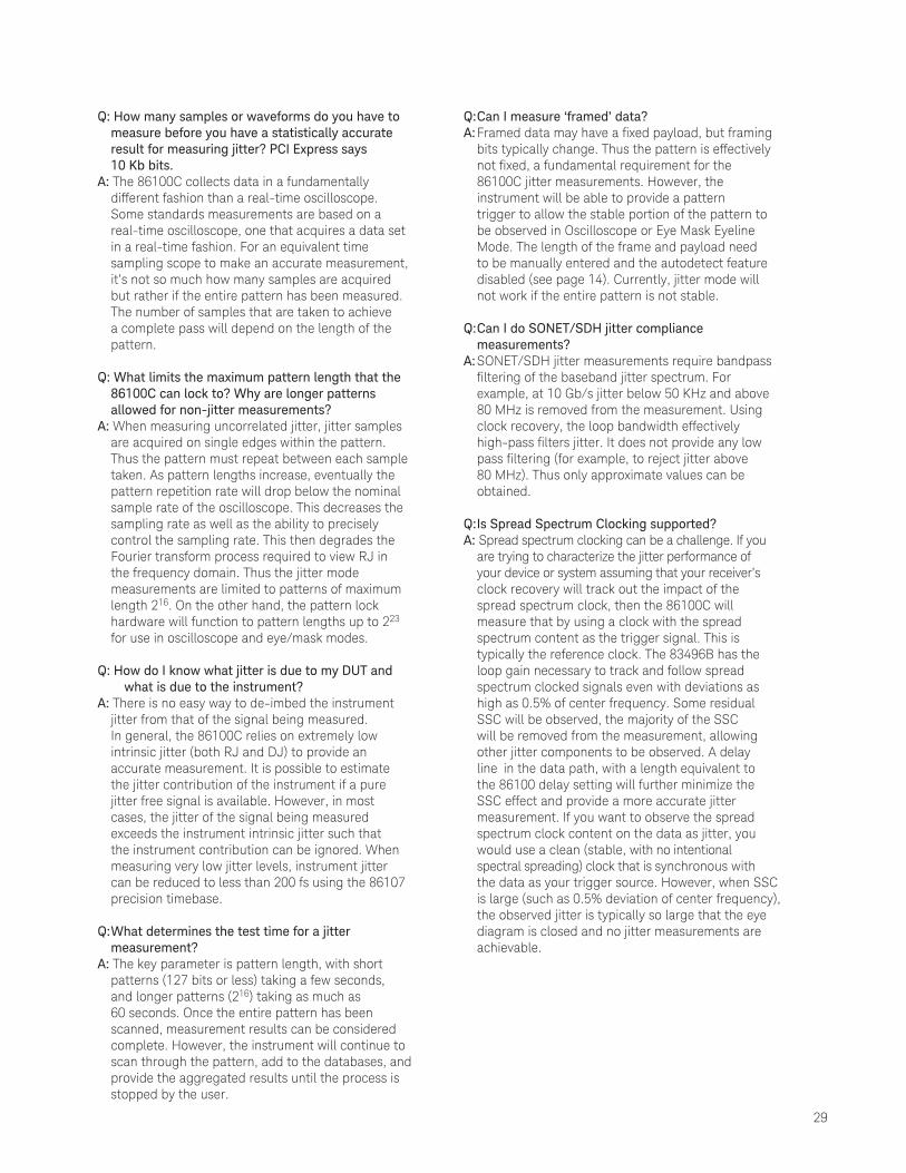
29

Q: Can I measure ‘framed’ data?A: Framed data may have a fixed payload, but framing bits typically change. Thus the pattern is effectively not fixed, a fundamental requirement for the 86100C jitter measurements. However, the instrument will be able to provide a pattern trigger to allow the stable portion of the pattern to be observed in Oscilloscope or Eye Mask Eyeline Mode. The length of the frame and payload need to be manually entered and the autodetect feature disabled (see page 14). Currently, jitter mode will not work if the entire pattern is not stable.

Q: Can I do SONET/SDH jitter compliance measurements?A: SONET/SDH jitter measurements require bandpass filtering of the baseband jitter spectrum. For example, at 10 Gb/s jitter below 50 KHz and above 80 MHz is removed from the measurement. Using clock recovery, the loop bandwidth effectively high-pass filters jitter. It does not provide any low pass filtering (for example, to reject jitter above 80 MHz). Thus only approximate values can be obtained.

Q: Is Spread Spectrum Clocking supported?A: Spread spectrum clocking can be a challenge. If you are trying to characterize the jitter performance of your device or system assuming that your receiver’s clock recovery will track out the impact of the spread spectrum clock, then the 86100C will measure that by using a clock with the spread spectrum content as the trigger signal. This is typically the reference clock. The 83496B has the loop gain necessary to track and follow spread spectrum clocked signals even with deviations as high as 0.5% of center frequency. Some residual SSC will be observed, the majority of the SSC will be removed from the measurement, allowing other jitter components to be observed. A delay line in the data path, with a length equivalent to the 86100 delay setting will further minimize the SSC effect and provide a more accurate jitter measurement. If you want to observe the spread spectrum clock content on the data as jitter, you would use a clean (stable, with no intentional spectral spreading) clock that is synchronous with the data as your trigger source. However, when SSC is large (such as 0.5% deviation of center frequency), the observed jitter is typically so large that the eye diagram is closed and no jitter measurements are achievable.

Q: How many samples or waveforms do you have to measure before you have a statistically accurate result for measuring jitter? PCI Express says 10 Kb bits.A: The 86100C collects data in a fundamentally different fashion than a real-time oscilloscope. Some standards measurements are based on a real-time oscilloscope, one that acquires a data set in a real-time fashion. For an equivalent time sampling scope to make an accurate measurement, it’s not so much how many samples are acquired but rather if the entire pattern has been measured. The number of samples that are taken to achieve a complete pass will depend on the length of the pattern.

Q: What limits the maximum pattern length that the 86100C can lock to? Why are longer patterns allowed for non-jitter measurements?A: When measuring uncorrelated jitter, jitter samples are acquired on single edges within the pattern. Thus the pattern must repeat between each sample taken. As pattern lengths increase, eventually the pattern repetition rate will drop below the nominal sample rate of the oscilloscope. This decreases the sampling rate as well as the ability to precisely control the sampling rate. This then degrades the Fourier transform process required to view RJ in the frequency domain. Thus the jitter mode measurements are limited to patterns of maximum length 216. On the other hand, the pattern lock hardware will function to pattern lengths up to 223 for use in oscilloscope and eye/mask modes.

Q: How do I know what jitter is due to my DUT and what is due to the instrument?A: There is no easy way to de-imbed the instrument jitter from that of the signal being measured. In general, the 86100C relies on extremely low intrinsic jitter (both RJ and DJ) to provide an accurate measurement. It is possible to estimate the jitter contribution of the instrument if a pure jitter free signal is available. However, in most cases, the jitter of the signal being measured exceeds the instrument intrinsic jitter such that the instrument contribution can be ignored. When measuring very low jitter levels, instrument jitter can be reduced to less than 200 fs using the 86107 precision timebase.

Q: What determines the test time for a jitter measurement?A: The key parameter is pattern length, with short patterns (127 bits or less) taking a few seconds, and longer patterns (216) taking as much as 60 seconds. Once the entire pattern has been scanned, measurement results can be considered complete. However, the instrument will continue to scan through the pattern, add to the databases, and provide the aggregated results until the process is stopped by the user.

30

Q. Will using a clock recovery module in the DCA affect my jitter measurements?A: Triggering with a recovered clock will affect the measurements. The loop bandwidth of the clock recovery system effectively high-pass filters the jitter, as jitter within the loop bandwidth is common to the trigger and the data and is not observed. This is often desirable and required in some test standards.

Q. How do I determine how much bandwidth (which DCA module) I need in order to make accurate jitter measurements?A: Insufficient bandwidth can lead to additional ISI jitter and edge distortion, degrading jitter measurements. In general, the channel bandwidth should be approximately double the data rate of the signal (assumes NRZ data). Channel noise increases with bandwidth, which can also affect jitter measurement accuracy, so the bandwidth should not be blindly set to the largest value available. Channel bandwidth depends on what plug-in module is used. Also, the bandwidth is adjustable in the channel menu.

Q. Can I determine the frequency of the measured periodic jitter?A: While in jitter mode select the “frequency” tab to display the spectral components of periodic and subrate jitter.

Q. Why is the skew feature disabled in jitter mode?A: The jitter measurement technique requires precision control and location of when and where amplitude samples are taken to allow an accurate amplitude to jitter transfer function. Electronic skew adjust degrades jitter measurement accuracy. However, external skew (hardware cable adjustments) are allowable.

31 | Keysight | Precision Jitter Analysis Using the Keysight 86100C DCA-J - Application Note

This information is subject to change without notice.© Keysight Technologies, 2017Published in USA, December 2, 20175989-1146ENwww.keysight.com

For more information on Keysight Technologies’ products, applications or services, please contact your local Keysight office. The complete list is available at:www.keysight.com/find/contactus

Americas Canada (877) 894 4414Brazil 55 11 3351 7010Mexico 001 800 254 2440United States (800) 829 4444

Asia PacificAustralia 1 800 629 485China 800 810 0189Hong Kong 800 938 693India 1 800 11 2626Japan 0120 (421) 345Korea 080 769 0800Malaysia 1 800 888 848Singapore 1 800 375 8100Taiwan 0800 047 866Other AP Countries (65) 6375 8100

Europe & Middle EastAustria 0800 001122Belgium 0800 58580Finland 0800 523252France 0805 980333Germany 0800 6270999Ireland 1800 832700Israel 1 809 343051Italy 800 599100Luxembourg +32 800 58580Netherlands 0800 0233200Russia 8800 5009286Spain 800 000154Sweden 0200 882255Switzerland 0800 805353

Opt. 1 (DE)Opt. 2 (FR)Opt. 3 (IT)

United Kingdom 0800 0260637

For other unlisted countries:www.keysight.com/find/contactus(BP-9-7-17)

DEKRA CertifiedISO9001 Quality Management System

www.keysight.com/go/qualityKeysight Technologies, Inc.DEKRA Certified ISO 9001:2015Quality Management System

Evolving Since 1939Our unique combination of hardware, software, services, and people can help you reach your next breakthrough. We are unlocking the future of technology. From Hewlett-Packard to Agilent to Keysight.

myKeysightwww.keysight.com/find/mykeysightA personalized view into the information most relevant to you.

http://www.keysight.com/find/emt_product_registrationRegister your products to get up-to-date product information and find warranty information.

Keysight Serviceswww.keysight.com/find/serviceKeysight Services can help from acquisition to renewal across your instrument’s lifecycle. Our comprehensive service offerings—one-stop calibration, repair, asset management, technology refresh, consulting, training and more—helps you improve product quality and lower costs.

Keysight Assurance Planswww.keysight.com/find/AssurancePlansUp to ten years of protection and no budgetary surprises to ensure your instruments are operating to specification, so you can rely on accurate measurements.

Keysight Channel Partnerswww.keysight.com/find/channelpartnersGet the best of both worlds: Keysight’s measurement expertise and product breadth, combined with channel partner convenience.