Embed Size (px)
Citation preview

Kernel Interpolation for Scalable StructuredGaussian Processes (KISS-GP)
Andrew Gordon WilsonCarnegie Mellon University
Hannes NickischPhilips Research Hamburg
Abstract
We introduce a new structured kernel interpolation (SKI) framework, whichgeneralises and unifies inducing point methods for scalable Gaussian processes(GPs). SKI methods produce kernel approximations for fast computationsthrough kernel interpolation. The SKI framework clarifies how the quality ofan inducing point approach depends on the number of inducing (aka interpola-tion) points, interpolation strategy, and GP covariance kernel. SKI also providesa mechanism to create new scalable kernel methods, through choosing differentkernel interpolation strategies. Using SKI, with local cubic kernel interpolation,we introduce KISS-GP, which is 1) more scalable than inducing point alterna-tives, 2) naturally enables Kronecker and Toeplitz algebra for substantial addi-tional gains in scalability, without requiring any grid data, and 3) can be usedfor fast and expressive kernel learning. KISS-GP costs O(n) time and storagefor GP inference. We evaluate KISS-GP for kernel matrix approximation, kernellearning, and natural sound modelling.
1 Introduction
Gaussian processes (GPs) are exactly the types of models we want to apply to big data:flexible function approximators, capable of using the information in large datasetsto learn intricate structure through interpretable and expressive covariance kernels.However, O(n3) and O(n2) computation and storage requirements limit GPs to allbut the smallest datasets, containing at most a few thousand training points n. Theirimpressive empirical successes thus far are only a glimpse of what might be possible,if only we could overcome these computational limitations (Rasmussen, 1996).
Inducing point methods (Snelson and Ghahramani, 2006; Hensman et al., 2013;Quinonero-Candela and Rasmussen, 2005; Seeger, 2005; Smola and Bartlett, 2001;
1
arX
iv:1
503.
0105
7v1
[cs
.LG
] 3
Mar
201
5
Silverman, 1985) have been introduced to scale up Gaussian processes to larger data-sizes. These methods cost O(m2n + m3) computations and O(mn + m2) storage, form inducing points, and n training data points. Inducing methods are popular for theirgeneral purpose “out of the box” applicability, without requiring any special structurein the data. However, these methods are limited by requiring a small m� n numberof inducing inputs, which can cause a deterioration in predictive performance, and theinability to perform expressive kernel learning (Wilson et al., 2014).
Structure exploiting approaches for scalability, such as Kronecker (Saatchi, 2011) orToeplitz (Cunningham et al., 2008) methods, have orthogonal advantages to inducingpoint methods. These methods exploit the existing structure in the covariance kernelfor highly accurate and scalable inference, and can be used for flexible kernel learningon large datasets (Wilson et al., 2014). However, Kronecker methods require that in-puts (predictors) are on a multidimensional lattice (a Cartesian product grid), whichmakes them inapplicable to most datasets. Although Wilson et al. (2014) has extendedKronecker methods for partial grid structure, these extensions do not apply to arbitrar-ily located inputs. Likewise, the Kronecker based approach in Luo and Duraiswami(2013) involves costly rank-1 updates and is not generally applicable for arbitrarilylocated inputs. Toeplitz methods are similarly restrictive, requiring that the data areon a regularly spaced 1D grid.
It is tempting to assume we could place inducing points on a grid, and then take advan-tage of Kronecker or Toeplitz structure for further gains in scalability. However, thisnaive approach only helps reduce the m3 complexity term in inducing point methods,and not the more critical m2n term, which arises from a matrix of cross covariancesbetween training and inducing inputs.
In this paper, we introduce a new unifying framework for inducing point methods,called structured kernel interpolation (SKI). This framework allows us to improve thescalability and accuracy of fast kernel methods, and to naturally combine the advan-tages of inducing point and structure exploiting approaches. In particular,
• We show how current inducing point methods can be interpreted as performinga global GP interpolation on a true underlying kernel to create an approximatekernel for scalable computations, as part of a more general family of structuredkernel interpolation methods.
• The SKI framework helps us understand how the accuracy and efficiency of aninducing point method is affected by the number of inducing points m, the choiceof kernel, and the choice of interpolation method. Moreover, by choosing differentinterpolation strategies for SKI, we can create new inducing point methods.
• We introduce a new inducing point method, KISS-GP, which uses local cubicand inverse distance weighting interpolation strategies to create a sparse approx-imation to the cross covariance matrix between the inducing points and originaltraining points. This method can naturally be combined with Kronecker and
2
Toeplitz algebra to allow for m � n inducing points, and further gains in scal-ability. When exploiting Toeplitz structure KISS-GP requires O(n + m logm)computations and O(n + m) storage. When exploiting Kronecker structure,KISS-GP requires O(n + Pm1+1/P ) computations and O(n + Pm2/P ) storage,for P > 1 dimensional inputs.
• KISS-GP can be viewed as lifting the grid restrictions in Toeplitz and Kroneckermethods, so that one can use arbitrarily located inputs.
• We show that the ability for KISS-GP to efficiently use a large number of induc-ing points enables expressive kernel learning, and orders of magnitude greateraccuracy and efficiency over popular alternatives such as FITC (Snelson andGhahramani, 2006).
• We have implemented code as an extension to the GPML toolbox (Rasmussenand Nickisch, 2010).
• Overall, the simplicity and generality of the SKI framework makes it easy todesign scalable Gaussian process methods with high accuracy and low computa-tional costs.
We start in section 2 with background on Gaussian processes (section 2.1), induc-ing point methods (section 2.2), and structure exploiting methods (section 2.3). Wethen introduce the structured kernel interpolation (SKI) framework, and the KISS-GPmethod, in section 3. In section 4 we conduct experiments on kernel matrix recon-struction, kernel learning, and natural sound modelling. We conclude in section 5.
2 Background
2.1 Gaussian Processes
We provide a brief review of Gaussian processes (Rasmussen and Williams, 2006), andthe associated computational requirements for inference and learning. Throughout weassume we have a dataset D of n input (predictor) vectors X = {x1, . . . ,xn}, each ofdimension D, corresponding to a n× 1 vector of targets y = (y(x1), . . . , y(xn))>.
A Gaussian process (GP) is a collection of random variables, any finite number ofwhich have a joint Gaussian distribution. Using a GP, we can define a distributionover functions f(x) ∼ GP(µ, k), meaning that any collection of function values f hasa joint Gaussian distribution:
f = f(X) = [f(x1), . . . , f(xn)]> ∼ N (µ, K) . (1)
The n × 1 mean vector µi = µ(xi), and n × n covariance matrix Kij = k(xi,xj),are defined by the user specified mean function µ(x) = E[f(x)] and covariance kernel
3

k(x,x′) = cov(f(x), f(x′)) of the Gaussian process. The smoothness and generalisationproperties of the GP are encoded by the covariance kernel and its hyperparameters θ.For example, the popular RBF covariance function, with length-scale hyperparameter`, has the form
kRBF(x,x′) = exp(−0.5||x− x′||2/`2) . (2)
If the targets y(x) are modelled by a GP with additive Gaussian noise, e.g., y(x)|f(x) ∼N (y(x); f(x), σ2), the predictive distribution at n∗ test points X∗ is given by
f∗|X∗,X,y,θ, σ2 ∼ N (f∗, cov(f∗)) , (3)
f∗ = µX∗ +KX∗,X [KX,X + σ2I]−1y ,
cov(f∗) = KX∗,X∗ −KX∗,X [KX,X + σ2I]−1KX,X∗ .
KX∗,X , for example, denotes the n∗×n matrix of covariances between the GP evaluatedat X∗ and X. µX∗ is the n∗× 1 mean vector, and KX,X is the n×n covariance matrixevaluated at training inputs X. All covariance matrices implicitly depend on the kernelhyperparameters θ.
We can analytically marginalise the Gaussian process f(x) to obtain the marginallikelihood of the data, conditioned only on the covariance hyperparameters θ:
log p(y|θ) ∝ −[
model fit︷ ︸︸ ︷y>(Kθ + σ2I)−1y+
complexity penalty︷ ︸︸ ︷log |Kθ + σ2I|] . (4)
Eq. (4) nicely separates into automatically calibrated model fit and complexity terms(Rasmussen and Ghahramani, 2001), and can be optimized to learn the kernel hyper-parameters θ, or used to integrate out θ via MCMC (Rasmussen, 1996).
The computational bottleneck in using Gaussian processes is solving a linear system(K+σ2I)−1y (for inference), and log |K+σ2I| (for hyperparameter learning). For thispurpose, standard procedure is to compute the Cholesky decomposition of K, requiringO(n3) operations and O(n2) storage. Afterwards, the predictive mean and variancerespectively cost O(n) and O(n2) for a single test point x∗.
2.2 Inducing Point Based Sparse Approximations
Many popular approaches to scaling up GP inference belong to a family of induc-ing point methods (Quinonero-Candela and Rasmussen, 2005). These methods canbe viewed as replacing the exact kernel k(x, z) by an approximation k(x, z) for fastcomputations.
For example, the prominent subset of regressors (SoR) (Silverman, 1985) and fullyindependent training conditional (FITC) (Snelson and Ghahramani, 2006) methods
4
use the approximate kernels
kSoR(x, z) = Kx,UK−1U,UKU,z , (5)
kFITC(x, z) = kSoR(x, z) + δxz
(k(x, z)− kSoR(x, z)
), (6)
for a set of m inducing points U = [ui]i=1...m. Kx,U , K−1U,U , and KU,z are generated
from the exact kernel k(x, z). While SoR yields an n × n covariance matrix KSoR ofrank at most m, corresponding to a degenerate (finite basis) Gaussian process, FITCleads to a full rank covariance matrix KFITC due to its diagonal correction. As a result,FITC is a more faithful approximation and is preferred in practice. Note that the exactuser-specified kernel, k(x, z), will be parametrized by θ, and therefore kernel learningin an inducing point method takes place by, e.g., optimizing the SoR or FITC marginallikelihoods with respect to θ.
These approximate kernels give rise to O(m2n + m3) computations and O(mn + m2)storage for GP inference and learning (Quinonero-Candela and Rasmussen, 2005), afterwhich the GP predictive mean and variance cost O(m) and O(m2) per test case. Tosee practical efficiency gains over standard inference procedures, one is constrained tochoose m � n, which often leads to a severe deterioration in predictive performance,and an inability to perform expressive kernel learning (Wilson et al., 2014).
2.3 Fast Structure Exploiting Inference
Kronecker and Toeplitz methods exploit the existing structure of the GP covariancematrix K to scale up inference and learning without approximations.
2.3.1 Kronecker Methods
We briefly review Kronecker methods. A full introduction is provided in chapter 5 ofSaatchi (2011).
If we have multidimensional inputs on a Cartesian grid, x ∈ X1 × · · · × XP , and aproduct kernel across grid dimensions, k(xi,xj) =
∏Pp=1 k(x
(p)i ,x
(p)j ), then the m ×m
covariance matrix K can be expressed as a Kronecker product K = K1 ⊗ · · · ⊗ KP
(the number of grid points m =∏P
i=1 np is a product of the number of points np
per grid dimension). It follows that we can efficiently find the eigendecomposition ofK = QV Q> by separately computing the eigendecomposition of each of K1, . . . , KP .One can similarly exploit Kronecker structure for fast matrix vector products (Wilsonet al., 2014).
Fast eigendecompositions and matrix vector products of Kronecker matrices allow us toefficiently evaluate (K+σ2I)−1y and log |K+σ2I| for scalable and exact inference and
5
learning with GPs. Specifically, given an eigendecomposition of K as QV Q>, we canwrite (K + σ2I)−1y = (QV Q> + σ2I)−1y = Q(V + σ2I)−1Q>y, and log |K + σ2I| =∑
i log(Vii + σ2). V is a diagonal matrix of eigenvalues, so inversion is trivial. Q,an orthogonal matrix of eigenvectors, also decomposes as a Kronecker product, whichenables fast matrix vector products. Overall, inference and learning cost O(Pm1+1/P )
operations (for P > 1) and O(Pm2P ) storage (Saatchi, 2011; Wilson et al., 2014).
While product kernels can be easily constructed, and popular kernels such as the RBFkernel of Eq. (2) already have product structure, requiring a multidimensional inputgrid can be a severe constraint.
Wilson et al. (2014) extend Kronecker methods to datasets with only partial grid struc-ture – e.g., images with random missing pixels, or spatiotemporal grids with missingdata due to water. They complete a partial grid with virtual observations, and use adiagonal noise covariance matrix A which ignores the effects of these virtual observa-tions: K(n) + σ2I → K(m) +A, where K(n) is an n× n covariance matrix formed fromthe original dataset with n datapoints, and K(m) is the covariance matrix after augmen-tation from virtual inputs. Although we cannot efficiently eigendecompose K(m) + A,we can take matrix vector products (K(m) +A)y(m) efficiently, since K(m) is Kroneckerand A is diagonal. We can thus compute (K(m) + A)−1y(m) = (K(n) + σ2I)−1y(n) towithin machine precision, and perform efficient inference, using iterative methods suchas linear conjugate gradients, which only involve matrix vector products.
To evaluate the marginal likelihood in Eq. (4), for kernel learning, we must also com-pute log |K(n) +σ2I|, where K(n) is an n×n covariance matrix formed from the originaldataset with n datapoints. Wilson et al. (2014) propose to approximate the eigenval-
ues λ(n)i of K(n) using the largest n eigenvalues λi of K(m), the Kronecker covariance
matrix formed from the completed grid, which can be eigendecomposed efficiently. Inparticular,
log |K(n) + σ2I| =n∑
i=1
log(λ(n)i + σ2) ≈
n∑i=1
log(n
mλi + σ2) .
Theorem 3.4 of Baker (1977) proves this eigenvalue approximation is asymptoticallyconsistent (e.g., converges in the limit of large n), so long as the observed inputs arebounded by the complete grid. Williams and Shawe-Taylor (2003) also show that onecan bound the true eigenvalues by their approximation using PCA. Notably, only thelog determinant (complexity penalty) term in the marginal likelihood undergoes a smallapproximation. Wilson et al. (2014) show that, in practice, this approximation can behighly effective for fast and expressive kernel learning.
However, the extensions in Wilson et al. (2014) are only efficient if the input space haspartial grid structure, and do not apply in general settings.
6
2.3.2 Toeplitz Methods
Toeplitz and Kronecker methods are complementary. K is a Toeplitz covariance matrixif it is generated from a stationary covariance kernel, k(x,x′) = k(x− x′), with inputsx on a regularly spaced one dimensional grid. Toeplitz matrices are constant alongtheir diagonals: Ki,j = Ki+1,j+1 = k(xi − xj).
One can embed Toeplitz matrices into circulant matrices, to perform fast matrix vectorproducts using fast Fourier transforms, e.g., Wilson (2014). One can then use linearconjugate gradients to solve linear systems (K+σ2I)−1y in O(m logm) operations andO(m) storage, for m grid datapoints. Turner (2010) and Cunningham et al. (2008)contain examples of Toeplitz methods applied to GPs.
3 Structured Kernel Interpolation
We wish to ease the large O(n3) computations and O(n2) storage associated withGaussian processes, while retaining model flexibility and general applicability.
Inducing point approaches (section 2.2) to scalability are popular because they can beapplied “out of the box”, without requiring special structure in the data. However,with a small number of inducing points, these methods suffer from a major deterio-ration in predictive accuracy, and the inability to perform expressive kernel learning(Wilson et al., 2014), which will be most valuable on large datasets. On the other hand,structure exploiting approaches (section 2.3) are compelling because they provide in-credible gains in scalability, with essentially no losses in predictive accuracy. But therequirement of an input grid makes these methods inapplicable to most problems.
Looking at equations (5) and (6), it is tempting to try placing the locations of theinducing points U on a grid, in the SoR or FITC methods, and then exploit eitherKronecker or Toeplitz algebra to efficiently solve linear systems involving K−1
U,U . While
this naive approach would reduce the O(m3) complexity associated with K−1U,U , that is
not the dominant term for computations with inducing point methods – rather, it isthe O(m2n) computations associated with the product KX,UK
−1U,U .
We observe, however, that we can approximate the n × m matrix KX,U of cross co-variances for the kernel evaluated at the training and inducing inputs X and U , byinterpolating on the m ×m covariance matrix KU,U . For example, if we wish to esti-mate k(xi,uj), for input point xi and inducing point uj, we can start by finding thetwo inducing points ua and ub which most closely bound xi: ua ≤ xi ≤ ub (initiallyassuming D = 1 and a Toeplitz KU,U from a regular grid U , for simplicity). We canthen form k(xi,uj) = wik(ua,uj) + (1−wi)k(ub,uj), with linear interpolation weightswi and (1 − wi), which represent the relative distances from xi to points ua and ub.
7

More generally, we form
KX,U ≈ WKU,U , (7)
where W is an n × m matrix of interpolation weights. We observe that W can beextremely sparse. For local linear interpolation, W contains only c = 2 non-zeroentries per row – the interpolation weights – which sum to 1. For greater accuracy, wecan use local cubic interpolation (Keys, 1981) on equispaced grids, in which case Whas c = 4 non-zero entries per row. For general rectilinear grids U (without regularspacing), we can use inverse distance weighting (Shepard, 1968) with c = 2 non-zeroweights per row of W .
Substituting our expression for KX,U in Eq. (7) into the SoR approximation for KX,X ,we find:
KX,XSoR≈ KX,UK
−1U,UKU,X
Eq. (7)≈ WKU,UK
−1U,UKU,UW
>
= WKU,UW> = KSKI . (8)
We name this general approach to approximating GP kernel functions structured kernelinterpolation (SKI). Although we have made use of the SoR approximation as anexample, SKI can be applied to essentially any inducing point method, such as FITC.1,2
We can compute fast matrix vector products KSKIy. If we do not exploit Toeplitz orKronecker structure in KU,U , a matrix vector product costs O(n + m2) computationsand O(n+m2) storage (matrix vector products with KU,U cost O(m2) computations,and with sparse W cost O(n), with the same storage requirements). If we exploit
Kronecker structure, we only require O(Pm1+1/P ) computations and O(n + Pm2P )
storage (matrix vector products with KU,U now cost O(Pm1+1/P ) computations and
O(Pm2P ) storage). If we exploit Toeplitz structure, we only require O(n + m logm)
computations and O(n + m) storage (a matrix vector product with KU,U now costsO(m logm) computations and O(m) storage).
Inference proceeds by solving K−1SKIy through linear conjugate gradients, which only
requires matrix vector products and a small number j � n of iterations for conver-gence to within machine precision. To compute log |KSKI|, for the marginal likelihoodevaluations used in kernel learning, one can follow the approximation of Wilson et al.(2014), described in section 2.3.1, where KU,U takes the role of K(m), and virtual ob-servations are not required. Alternatively, we can use the ability to take fast matrixvector products with KSKI in standard eigenvalue solvers to efficiently compute the logdeterminant exactly. We can also form an accurate approximation by selectively com-puting the largest and smallest eigenvalues. This alternative approach is not possible in
1Combining with the SoR approximate k(x, z), one can naively use kSKI(x, z) = w>xKU,Uwz, where
wx,wz ∈ Rm are interpolation vectors for points x and z; however, when wx 6= wz, it makes mostsense to perform local interpolation on KU,z directly.
2Later we discuss the logistics of combining with FITC.
8
Wilson et al. (2014) since in that case one cannot take fast matrix vector products withK(n). In either fast approach, the computional complexity for learning is no greaterthan for inference.
In short, even if we choose not to exploit potential Kronecker or Toeplitz structurein KU,U , inference and learning in SKI are accelerated over standard inducing pointapproaches. However, unlike with the data inputs, X, which are fixed, we are free tochoose the locations of the latent inducing points U , and therefore we can easily create(e.g., Toeplitz or Kronecker) structure in KU,U which might not exist in KX,X . In theSKI formalism, we can uniquely exploit this structure for substantial additional gainsin efficiency, and the ability to use an unprecedented number of inducing points, whilelifting any grid requirements for the training inputs X.
Although here we have made use of the SoR approximation in Eq. (8), we could triviallyapply the FITC diagonal correction (section 2.2), or combine with other approaches.However, within the SKI framework, the diagonal correction of FITC does not have asmuch value: KSKI can easily be full rank and still have major computational benefits,using m > n. In conventional inducing approximations, one would never set m > n,since this would be less efficient than exact Gaussian process inference.
Finally, we can understand all of these inducing approaches as part of a general struc-tured kernel interpolation (SKI) framework. The predictive mean f∗ in Eq. (3) of anoise-free, zero mean GP (σ = 0, µ(x) ≡ 0) is linear in two ways: on the one hand, asa wX(x∗) = K−1
X,XKX,x∗ weighted sum of the observations y, and on the other hand as
an α = K−1X,Xy weighted sum of training-test cross-covariances KX,x∗ :
f∗ = y>wX(x∗) = α>KX,x∗ . (9)
If we are to perform a noise free zero-mean GP regression on the kernel itself, such thatwe have data D = (ui, k(ui,x))mi=1, then we recover the SoR kernel kSoR(x, z) of equa-tion (5) as the predictive mean of the GP at test point x∗ = z. This finding providesa new unifying perspective on inducing point approaches: all conventional inducingpoint methods, such as SoR and FITC, can be re-derived as performing a zero-meanGaussian process interpolation on the true kernel. Indeed, we could write interpolationpoints instead of inducing points. The n × m interpolation weight matrix W , in allconventional cases, will have all non-zero entries, which incurs great computationalexpenses. And, computional considerations aside, it is not ideal for inducing pointmethods to perform a zero-mean GP regression on a covariance kernel. For example,since popular kernels are often strictly positive – neither zero-mean, nor accuratelycharacterized by a Gaussian distribution – conventional inducing point methods willtend to underestimate covariances.
The SKI interpretation of inducing point methods provides a mechanism to createnew inducing point approaches. By replacing global GP kernel interpolation withlocal inverse distance weighting or cubic interpolation, as part of our SKI framework,
9
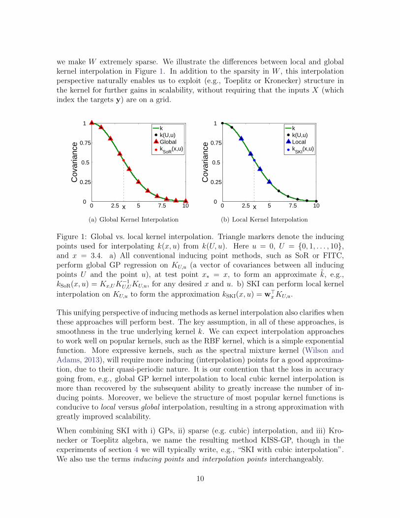
we make W extremely sparse. We illustrate the differences between local and globalkernel interpolation in Figure 1. In addition to the sparsity in W , this interpolationperspective naturally enables us to exploit (e.g., Toeplitz or Kronecker) structure inthe kernel for further gains in scalability, without requiring that the inputs X (whichindex the targets y) are on a grid.
0 2.5 5 7.5 100
0.25
0.5
0.75
1
Cov
aria
nce
kk(U,u)Globalk
SoR(x,u)
x
(a) Global Kernel Interpolation
0 2.5 5 7.5 100
0.25
0.5
0.75
1
Cov
aria
nce
kk(U,u)Localk
SKI(x,u)
x
(b) Local Kernel Interpolation
Figure 1: Global vs. local kernel interpolation. Triangle markers denote the inducingpoints used for interpolating k(x, u) from k(U, u). Here u = 0, U = {0, 1, . . . , 10},and x = 3.4. a) All conventional inducing point methods, such as SoR or FITC,perform global GP regression on KU,u (a vector of covariances between all inducingpoints U and the point u), at test point x∗ = x, to form an approximate k, e.g.,kSoR(x, u) = Kx,UK
−1U,UKU,u, for any desired x and u. b) SKI can perform local kernel
interpolation on KU,u to form the approximation kSKI(x, u) = w>xKU,u.
This unifying perspective of inducing methods as kernel interpolation also clarifies whenthese approaches will perform best. The key assumption, in all of these approaches, issmoothness in the true underlying kernel k. We can expect interpolation approachesto work well on popular kernels, such as the RBF kernel, which is a simple exponentialfunction. More expressive kernels, such as the spectral mixture kernel (Wilson andAdams, 2013), will require more inducing (interpolation) points for a good approxima-tion, due to their quasi-periodic nature. It is our contention that the loss in accuracygoing from, e.g., global GP kernel interpolation to local cubic kernel interpolation ismore than recovered by the subsequent ability to greatly increase the number of in-ducing points. Moreover, we believe the structure of most popular kernel functions isconducive to local versus global interpolation, resulting in a strong approximation withgreatly improved scalability.
When combining SKI with i) GPs, ii) sparse (e.g. cubic) interpolation, and iii) Kro-necker or Toeplitz algebra, we name the resulting method KISS-GP, though in theexperiments of section 4 we will typically write, e.g., “SKI with cubic interpolation”.We also use the terms inducing points and interpolation points interchangeably.
10
4 Experiments
We evaluate SKI for kernel matrix approximation (section 4.1), kernel learning (section4.2), and natural sound modelling (section 4.3).
We particularly compare with FITC (Snelson and Ghahramani, 2006), because 1)FITC is the most popular inducing point approach, 2) FITC has been shown to havesuperior predictive performance and similar efficiency to other inducing methods, andis generally recommended (Naish-Guzman and Holden, 2007; Quinonero-Candela et al.,2007), and 3) FITC is well understood, and thus FITC comparisons help elucidate thefundamental properties of SKI, which is our primary goal. However, we also providecomparisons with SoR, and SSGPR (Lazaro-Gredilla et al., 2010), a recent state of theart scalable GP method based on random projections with O(m2n) computations andO(m2) storage for m basis functions and n training points (see also Rahimi and Recht,2007; Le et al., 2013; Yang et al., 2015; Lu et al., 2014).
Furthermore, we focus on the ability for SKI to allow a relaxation of Kronecker andToeplitz methods to arbitrarily located inputs. Since Toeplitz methods are restrictedto 1D inputs, and Kronecker methods can only be used for low dimensional (D < 5)input spaces (Saatchi, 2011), we consider lower dimensional problems.
All experiments were performed on a 2011 MacBook Pro, with an Intel i5 2.3 GHzprocessor and 4 GB of RAM.
4.1 Covariance Matrix Reconstruction
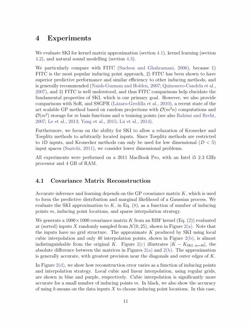
Accurate inference and learning depends on the GP covariance matrix K, which is usedto form the predictive distribution and marginal likelihood of a Gaussian process. Weevaluate the SKI approximation to K, in Eq. (8), as a function of number of inducingpoints m, inducing point locations, and sparse interpolation strategy.
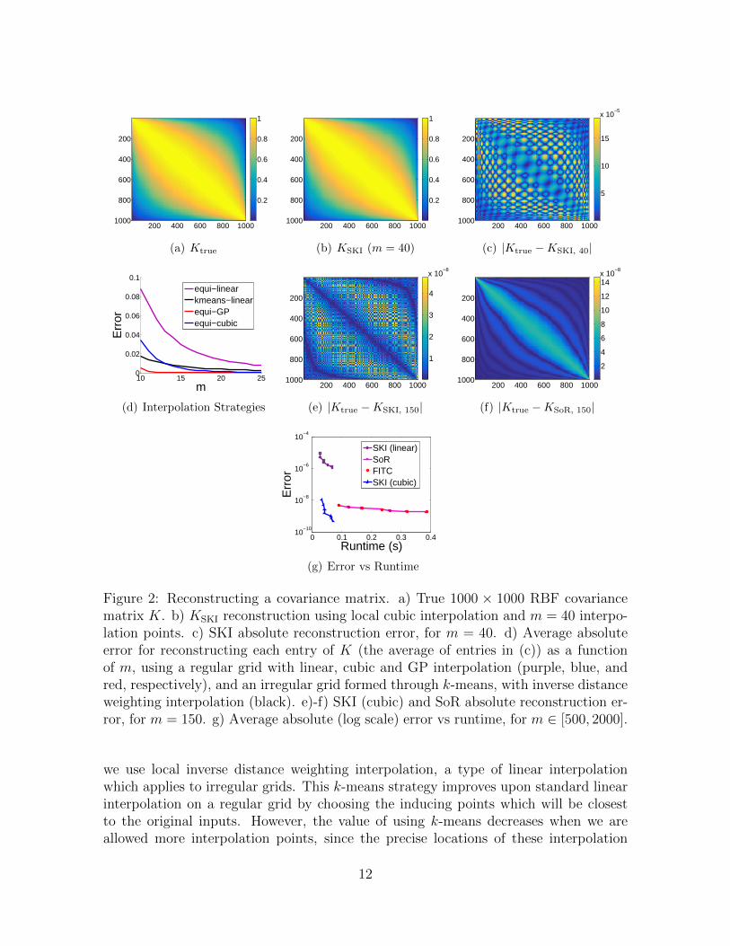
We generate a 1000×1000 covariance matrix K from an RBF kernel (Eq. (2)) evaluatedat (sorted) inputs X randomly sampled from N (0, 25), shown in Figure 2(a). Note thatthe inputs have no grid structure. The approximate K produced by SKI using localcubic interpolation and only 40 interpolation points, shown in Figure 2(b), is almostindistinguishable from the original K. Figure 2(c) illustrates |K − KSKI, m=40|, theabsolute difference between the matrices in Figures 2(a) and 2(b). The approximationis generally accurate, with greatest precision near the diagonals and outer edges of K.
In Figure 2(d), we show how reconstruction error varies as a function of inducing pointsand interpolation strategy. Local cubic and linear interpolation, using regular grids,are shown in blue and purple, respectively. Cubic interpolation is significantly moreaccurate for a small number of inducing points m. In black, we also show the accuracyof using k-means on the data inputs X to choose inducing point locations. In this case,
11
200 400 600 800 1000
200
400
600
800
1000
0.2
0.4
0.6
0.8
1
(a) Ktrue
200 400 600 800 1000
200
400
600
800
1000
0.2
0.4
0.6
0.8
1
(b) KSKI (m = 40)
200 400 600 800 1000
200
400
600
800
1000
5
10
15
x 10−5
(c) |Ktrue −KSKI, 40|
10 15 20 250
0.02
0.04
0.06
0.08
0.1
m
Err
or
equi−linearkmeans−linearequi−GPequi−cubic
(d) Interpolation Strategies
200 400 600 800 1000
200
400
600
800
1000
1
2
3
4
x 10−8
(e) |Ktrue −KSKI, 150|
200 400 600 800 1000
200
400
600
800
1000
2
4
6
8
10
12
14x 10
−8
(f) |Ktrue −KSoR, 150|
0 0.1 0.2 0.3 0.410
−10
10−8
10−6
10−4
Runtime (s)
Err
or
SKI (linear)SoRFITCSKI (cubic)
(g) Error vs Runtime
Figure 2: Reconstructing a covariance matrix. a) True 1000 × 1000 RBF covariancematrix K. b) KSKI reconstruction using local cubic interpolation and m = 40 interpo-lation points. c) SKI absolute reconstruction error, for m = 40. d) Average absoluteerror for reconstructing each entry of K (the average of entries in (c)) as a functionof m, using a regular grid with linear, cubic and GP interpolation (purple, blue, andred, respectively), and an irregular grid formed through k-means, with inverse distanceweighting interpolation (black). e)-f) SKI (cubic) and SoR absolute reconstruction er-ror, for m = 150. g) Average absolute (log scale) error vs runtime, for m ∈ [500, 2000].
we use local inverse distance weighting interpolation, a type of linear interpolationwhich applies to irregular grids. This k-means strategy improves upon standard linearinterpolation on a regular grid by choosing the inducing points which will be closestto the original inputs. However, the value of using k-means decreases when we areallowed more interpolation points, since the precise locations of these interpolation
12
points then becomes less critical, so long as we have general coverage of the inputdomain. Indeed, except for small m, cubic interpolation on a regular grid generallyoutperforms inverse distance weighting with k-means. Unsurprisingly, SKI with globalGP kernel interpolation (shown in red), which corresponds to the SoR approximation,is much more accurate than the other interpolation strategies for very small m� n.
However, global GP kernel interpolation is much less efficient than local cubic kernelinterpolation, and these accuracy differences quickly shrink with increases in m. Indeedin Figures 2(e) and 2(f) we see both reconstruction errors are similarly small for m =150, but qualitatively different. The error in the SoR reconstruction is concentratednear the diagonal, whereas the error in SKI with cubic interpolation never reaches thetop errors in SoR, and is more accurate than SoR near the diagonal, but is also morediffuse. This finding suggests that combining cubic interpolation with GP interpolationcould improve accuracy, if we account for the regions where each is strongest.
Ultimately, however, the important question is not which approximation is most ac-curate for a given m, but which approximation is most accurate for a given runtime(Chalupka et al., 2013). In Figure 2(g) we compare the accuracies and runtimes forSoR, FITC, and SKI with local linear and local cubic interpolation, for m ∈ [500, 2000]at m = 150 unit increments. m is sufficiently large that the differences in accuracybetween SoR and FITC are negligible. In general, the difference in going from SKIwith global GP interpolation (e.g., SoR or FITC) to SKI with local cubic interpola-tion (KISS-GP) is much more profound than the differences between SoR and FITC.Moreover, moving from local linear interpolation to local cubic interpolation providesa great boost in accuracy without noticeably affecting runtime. We also see that SKIwith local interpolation quickly picks up accuracy with increases in m, with local cubicinterpolation actually surpassing SoR and FITC in accuracy for a given m. Most im-portantly, for any given runtime, SKI with cubic interpolation is more accurate thanthe alternatives.
In this experiment we are testing the error and runtime for constructing an approximatecovariance matrix, but we are not yet performing inference with that covariance matrix,which is typically much more expensive, and where SKI will help the most. Moreover,we are not yet using Kronecker or Toeplitz structure to accelerate SKI.
4.2 Kernel Learning
We now test the ability for SKI to learn kernels from data using Gaussian processes. In-deed, SKI is intended to scale Gaussian processes to large datasets – and large datasetsprovide a distinct opportunity to discover rich statistical representations through kernellearning.
Popular inducing point methods, such as FITC, improve the scalability of Gaussianprocesses. However, Wilson et al. (2014) showed that these methods cannot typically
13
be used for expressive kernel learning, and are most suited to simple smoothing kernels.In other words, these scalable GP methods often miss out on structure learning, one ofthe greatest motivations for considering large datasets in the first place. This limitationarises because popular inducing methods require that the number of inducing pointsm� n, for computational tractability, which deprives us of the necessary informationto learn intricate kernels. SKI does not suffer from this problem, since we are free tochoose large m; in fact, m can be greater than n, while retaining significant efficiencygains over standard GPs.
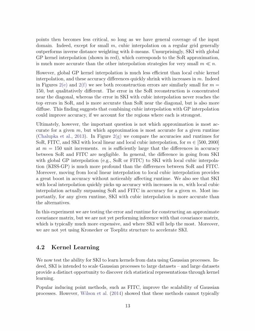
To test SKI and FITC for kernel learning, we sample data from a GP which usesa known ground truth kernel, and then attempt to learn this kernel from the data.In particular, we sample n = 10, 000 datapoints y from a Gaussian process with anintricate product kernel ktrue = k1k2 queried at inputs x ∈ R2 drawn from N (0, 4I) (theinputs have no grid structure). Each component kernel in the product operates on aseparate input dimension, as shown in green in Figure 3. Incidentally, n = 104 points isabout the upper limit of what we can sample from a multivariate Gaussian distributionwith a non-trivial covariance matrix. Even a single sample from a GP with this manydatapoints together with this sophisticated kernel is computationally intensive, taking1030 seconds in this instance. On the other hand, SKI can enable one to efficientlysample from extremely high dimensional (n > 1010) non-trivial multivariate Gaussiandistributions, which could be generally useful.3
To learn the kernel underlying the data, we optimize the SKI and FITC marginallikelihoods of a Gaussian process p(y|θ) with respect to the hyperparameters θ of aspectral mixture kernel, using non-linear conjugate gradients. In other words, the SKIand FITC kernels approximate a user specified (e.g., spectral mixture) kernel which isparametrized by θ, and to perform kernel learning we wish to learn θ from the data.Spectral mixture kernels (Wilson and Adams, 2013) form a basis for all stationarycovariance kernels, and are well-equipped for kernel learning. For SKI, we use cubicinterpolation and a 100×100 inducing point grid, equispaced in each input dimension.That is, we have as many inducing points m = 10, 000 as we have training datapoints.We use the same hyperparameter initialisation for each approach.
The results are shown in Figures 3(a) and 3(b). The true kernels are in green, the SKIreconstructions in blue, and the FITC reconstructions in red. SKI provides a strongapproximation, whereas FITC is unable to come near to reconstructing the true kernel.In this multidimensional example, SKI leverages Kronecker structure for efficiency, andhas a runtime of 2400 seconds (0.67 hours), using m = 10, 000 inducing points. FITC,on the other hand, has a runtime of 2.6× 10⁴ seconds (7.2 hours), with only m = 100inducing points. More inducing points with FITC breaks computational tractibility.
Even though the locations of the training points are randomly sampled, in SKI weexploited the Kronecker structure in the covariance matrix KU,U over the inducing
3Sampling would proceed, e.g., via WSKI[chol(K1)⊗ · · · ⊗ chol(Kp)]ν, ν ∼ N (0, I).
14
0 0.5 1−0.5
0
0.5
1
τ
Cor
rela
tion
TrueFITCSKI
0 0.5 1−0.2
0
0.2
0.4
0.6
0.8
τ
Cor
rela
tion
Figure 3: Kernel Learning. A product of two kernels (shown in green) was used tosample 10, 000 datapoints from a GP. From this data, we performed kernel learningusing SKI (cubic) and FITC, with the results shown in blue and red, respectively. Allkernels are a function of τ = x− x′ and are scaled by k(0).
points U , to reduce the cost of using 10, 000 inducing points to less than the cost ofusing 100 inducing points with FITC. FITC, and alternative inducing point methods,cannot effectively exploit Kronecker structure, because the non-sparse cross-covariancematrices KX,U and KU,X limit scaling to at best O(m2n), as per section 3.
4.3 Natural Sound Modelling
In section 4.2 we exploited multidimensional Kronecker structure in the SKI covariancematrix KU,U for scalability. For targets indexed by a set of 1D inputs, such as timeseries, we cannot exploit Kronecker structure for computational savings. However, byplacing the inducing points on a regular grid, we can create Toeplitz structure (section2.3.2) in KU,U which can be effectively exploited by SKI for additional scalability, butnot by popular alternatives.
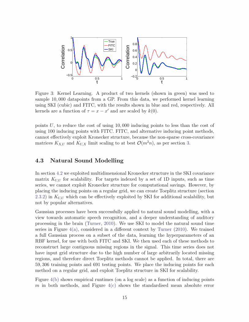
Gaussian processes have been successfully applied to natural sound modelling, with aview towards automatic speech recognition, and a deeper understanding of auditoryprocessing in the brain (Turner, 2010). We use SKI to model the natural sound timeseries in Figure 4(a), considered in a different context by Turner (2010). We traineda full Gaussian process on a subset of the data, learning the hyperparameters of anRBF kernel, for use with both FITC and SKI. We then used each of these methods toreconstruct large contiguous missing regions in the signal. This time series does nothave input grid structure due to the high number of large arbitrarily located missingregions, and therefore direct Toeplitz methods cannot be applied. In total, there are59, 306 training points and 691 testing points. We place the inducing points for eachmethod on a regular grid, and exploit Toeplitz structure in SKI for scalability.
Figure 4(b) shows empirical runtimes (on a log scale) as a function of inducing pointsm in both methods, and Figure 4(c) shows the standardised mean absolute error
15

0 1 2 3
−0.2
−0.1
0
0.1
0.2
Time (s)
Inte
nsity
(a) Natural Sound
2500 3000 3500 4000 4500 500010
0
101
102
103
m
Run
time
(s)
FITCSKI (cubic)
(b) Runtime vs m
100
101
102
103
0.2
0.3
0.4
0.5
0.6
0.7
0.8
Runtime (s)
SM
AE
(c) Error vs Runtime
Figure 4: Natural Sound Modelling. We reconstruct contiguous missing regions of anatural sound from n = 59, 306 observations. a) The observed data. b) Runtime forSKI and FITC (log scale) as a function of the number of inducing points m. c) TestingSMAE error as a function of (log scale) runtime.
(SMAE) on test points as a function of runtime (log scale) for each method.4 Form ∈ [2500, 5000] the runtime for SKI is essentially unaffected by increases in m, andhundreds of times faster than FITC, which does noticeably increase in runtime withm. Moreover, Figure 4(c) confirms our intuition that, for a given runtime, accuracylosses in going from GP kernel interpolation in FITC to the more simple cubic kernelinterpolation in the KISS-GP variant of SKI can be more than recovered by the gainin accuracy enabled through more inducing points. SKI has less than half of the errorat less than 1% the runtime cost of FITC. SKI is generally able to infer the correctcurvature in the function, while FITC, unable to use as many inducing points for anygiven runtime, tends to over-smooth the data. Eventually, however, adding more in-ducing points increases runtime without increasing accuracy. We also made predictionswith SSGPR (Lazaro-Gredilla et al., 2010), a recent state of the art approach to scal-able GP modelling, which requires O(m2n) computations and O(m2) storage, for mbasis functions and n training points. For a range of m ∈ [250, 1250], SSGPR hadSMAE ∈ [1.12, 1.23] and runtimes ∈ [310, 8400] seconds. Overall, SKI provides thebest reconstruction of the signal at the lowest runtime.
5 Discussion
We introduced a new structured kernel interpolation (SKI) framework, which gen-eralises and unifies inducing point methods for scalable Gaussian process inference.In particular, we showed how standard inducing point methods correspond to ker-nel approximations formed through global Gaussian process kernel interpolation. Bychanging to local cubic kernel interpolation, we introduced KISS-GP, a highly scalable
4SMAEmethod = MAEmethod / MAEempirical mean, so that the trivial solution of predicting with theempirical mean gives an SMAE of 1, and lower values correspond to better fits of the data.
16

inducing point method, which naturally combines with Kronecker and Toeplitz alge-bra for additional gains in scalability. Indeed we can view KISS-GP as relaxing thestringent grid assumptions in Kronecker and Toeplitz methods to arbitrarily locatedinputs. We showed that the ability for KISS-GP to efficiently handle a large number ofinducing points enabled expressive kernel learning and improved predictive accuracy,in addition to improved runtimes, over popular alternatives. In particular, for anygiven runtime, KISS-GP is orders of magnitude more accurate than the alternatives.Overall, simplicity and generality are major strengths of the SKI framework.
We have only begun to explore what could be done with this new framework. Struc-tured kernel interpolation opens the doors to a multitude of substantial new researchdirections. For example, one can create entirely new scalable Gaussian process modelsby changing interpolation strategies. These models could have remarkably differentproperties and applications. And we can use the perspective given by structured ker-nel interpolation to better understand the properties of any inducing point approach –e.g., which kernels are best approximated by a given approach, and how many inducingpoints will be needed for good performance. We can also combine new models gener-ated from SKI with the orthogonal benefits of recent stochastic variational inferencefor Gaussian processes. Moreover, the decomposition of the SKI covariance matrixinto a Kronecker product of Toeplitz matrices provides motivation to unify scalableKronecker and Toeplitz approaches. We hope that SKI will inspire many new modelsand unifying perspectives, and an improved understanding of scalable Gaussian processmethods.
References
Baker, C. T. (1977). The numerical treatment of integral equations. Clarendon Press.
Chalupka, K., Williams, C. K., and Murray, I. (2013). A framework for evaluatingapproximation methods for Gaussian process regression. The Journal of MachineLearning Research, 14(1):333–350.
Cunningham, J. P., Shenoy, K. V., and Sahani, M. (2008). Fast Gaussian process meth-ods for point process intensity estimation. In International Conference on MachineLearning.
Hensman, J., Fusi, N., and Lawrence, N. (2013). Gaussian processes for big data. InUncertainty in Artificial Intelligence (UAI). AUAI Press.
Keys, R. G. (1981). Cubic convolution interpolation for digital image processing. IEEETransactions on Acoustics, Speech and Signal Processing, 29(6):1153–1160.
Lazaro-Gredilla, M., Quinonero-Candela, J., Rasmussen, C., and Figueiras-Vidal, A.
17
(2010). Sparse spectrum Gaussian process regression. The Journal of MachineLearning Research, 11:1865–1881.
Le, Q., Sarlos, T., and Smola, A. (2013). Fastfood-computing Hilbert space expansionsin loglinear time. In Proceedings of the 30th International Conference on MachineLearning, pages 244–252.
Lu, Z., May, M., Liu, K., Garakani, A., D., G., Bellet, A., Fan, L., Collins, M.,Kingsbury, B., Picheny, M., and Sha, F. (2014). How to scale up kernel methods tobe as good as deep neural nets. Technical Report 1411.4000, arXiv. http://arxiv.
org/abs/1411.4000.
Luo, Y. and Duraiswami, R. (2013). Fast near-GRID Gaussian process regression. InProceedings of the Sixteenth International Conference on Artificial Intelligence andStatistics, pages 424–432.
Naish-Guzman, A. and Holden, S. (2007). The generalized fitc approximation. InAdvances in Neural Information Processing Systems, pages 1057–1064.
Quinonero-Candela, J. and Rasmussen, C. E. (2005). A unifying view of sparse approx-imate Gaussian process regression. Journal of Machine Learning Research (JMLR),6:1939–1959.
Quinonero-Candela, J., Rasmussen, C. E., and Williams, C. K. (2007). Approximationmethods for gaussian process regression. Large-scale kernel machines, pages 203–223.
Rahimi, A. and Recht, B. (2007). Random features for large-scale kernel machines. InNeural Information Processing Systems.
Rasmussen, C. E. (1996). Evaluation of Gaussian Processes and Other Methods forNon-linear Regression. PhD thesis, University of Toronto.
Rasmussen, C. E. and Ghahramani, Z. (2001). Occam’s razor. In Neural InformationProcessing Systems (NIPS).
Rasmussen, C. E. and Nickisch, H. (2010). Gaussian processes for machine learning(GPML) toolbox. Journal of Machine Learning Research (JMLR), 11:3011–3015.
Rasmussen, C. E. and Williams, C. K. I. (2006). Gaussian processes for MachineLearning. The MIT Press.
Saatchi, Y. (2011). Scalable Inference for Structured Gaussian Process Models. PhDthesis, University of Cambridge.
Seeger, M. (2005). Bayesian Gaussian process models: PAC-Bayesian generalisationerror bounds and sparse approximations. PhD thesis, University of Edinburgh.
18
Shepard, D. (1968). A two-dimensional interpolation function for irregularly-spaceddata. In Proceedings of the 1968 ACM National Conference, pages 517–524.
Silverman, B. W. (1985). Some aspects of the spline smoothing approach to non-parametric regression curve fitting. Journal of the Royal Statistical SocietyB, 47(1):1–52.
Smola, A. J. and Bartlett, P. (2001). Sparse greedy Gaussian process regression. InAdvances in Neural Information Processing Systems 13.
Snelson, E. and Ghahramani, Z. (2006). Sparse Gaussian processes using pseudo-inputs. In Advances in neural information processing systems (NIPS), volume 18,page 1257. MIT Press.
Turner, R. E. (2010). Statistical Models for Natural Sounds. PhD thesis, UniversityCollege London.
Williams, C. and Shawe-Taylor, J. (2003). The stability of kernel principal compo-nents analysis and its relation to the process eigenspectrum. Advances in neuralinformation processing systems, 15:383.
Wilson, A. G. (2014). Covariance kernels for fast automatic pattern discovery andextrapolation with Gaussian processes. PhD thesis, University of Cambridge.
Wilson, A. G. and Adams, R. P. (2013). Gaussian process kernels for pattern discoveryand extrapolation. International Conference on Machine Learning (ICML).
Wilson, A. G., Gilboa, E., Nehorai, A., and Cunningham, J. P. (2014). Fast kernellearning for multidimensional pattern extrapolation. In Advances in Neural Infor-mation Processing Systems.
Yang, Z., Smola, A. J., Song, L., and Wilson, A. G. (2015). A la carte - learning fastkernels. Artificial Intelligence and Statistics.
19