Max–Planck–Institut f ur biologische KybernetikMax Planck Institute for Biological Cybernetics

Technical Report No. 109

Kernel Hebbian Algorithm forIterative Kernel Principal

Component Analysis

Kwang In Kim,1 Matthias O. Franz,1 BernhardScholkopf1

June 2003

1 Department Scholkopf, email: kimki;mof;bs@tuebingen.mpg.de

This report is available in PDF–format via anonymous ftp at ftp://ftp.kyb.tuebingen.mpg.de/pub/mpi-memos/pdf/kha.pdf. The com-plete series of Technical Reports is documented at: http://www.kyb.tuebingen.mpg.de/techreports.html

Kernel Hebbian Algorithm for Iterative KernelPrincipal Component Analysis

Kwang In Kim, Matthias O. Franz, Bernhard Scholkopf

Abstract. A new method for performing a kernel principal component analysis is proposed. By kernelizingthe generalized Hebbian algorithm, one can iteratively estimate the principal components in a reproducing kernelHilbert space with only linear order memory complexity. The derivation of the method and preliminary applicationsin image hyperresolution are presented. In addition, we discuss the extension of the method to the online learningof kernel principal components.

1 Introduction

Kernel Principal Component Analysis (KPCA), a non-linear extension of PCA, is a powerful technique for extract-ing non-linear structure from data [1]. The basic idea is to map the input data into aReproducing Kernel HilbertSpace(RKHS) and then, to perform PCA in that space. While the direct computation of PCA in a RKHS is ingeneral infeasible due to the high dimensionality of that space, KPCA enables this by using kernel methods [2]and formulating PCA as the equivalentkernel eigenvalue problem. A problem of this approach is that it requiresto store and manipulate thekernel matrixthe size of which is square of the number of examples. This becomescomputationally expensive when the number of samples is large.

In this work, we adapt the Generalized Hebbian Algorithm (GHA), which was introduced as online algorithm forlinear PCA [3, 4], to perform PCA in RKHSs. Expanding the solution of GHA only in inner products of the samplesenables us to kernelize the GHA. The resultingKernel Hebbian Algorithm(KHA) estimates the eigenvectors ofthe kernel matrix with linear order memory complexity.

The capability of the KHA to handle large and high-dimensional datasets will be demonstrated in the contextof image hyperresolution where we project the images to be restored (i.e., the low resolution ones) into a spacespanned by the kernel principal components of a database of high-resolution images. The hyperresolution imageis then constructed from the projections by preimage techniques [5]. The resulting images show a considerablyricher structure than those obtained from linear PCA, since higher-order image statistics are taken into account.

This paper is organized as follows. Section 2 briefly introduces PCA, GHA, and KPCA. Section 3 formulatesthe KHA. Application results for image hyperresolution are presented in Section 4, while conclusions are drawnin Section 5.

2 Background

Principal component analysis. Given a set of centered observationsxk = RN , k = 1, . . . , l, and∑

lk=1xk = 0,

PCA diagonalizes the covariance matrix

C =1l

∑l

j=1xjxj

>.1

This is readily performed by solving the eigenvalue equation

λv = Cv

for eigenvaluesλ ≥ 0 and eigenvectorsvi ∈ RN \ 0.

1More precisely, the covariance matrix is defined as theE[xx>]; C is an estimate based on a finite set of examples.

1

Generalized Hebbian algorithm. From a computational point of view, it can be advantageous to solve theeigenvalue problem by iterative methods which do not need to compute and storeC directly. This is particularyuseful when the size ofC is large such that the memory complexity becomes prohibitive. Among the existingiterative methods for PCA, the generalized Hebbian algorithm (GHA) is of particular interest, since it does notonly provide a memory-efficient implementation but also has the inherent capability to adapt to time-varyingdistributions.

Let us define a matrixW(t) = (w1(t)>, . . . ,wr(t)>)>, wherer is the number of eigenvectors considered andwi(t) ∈ RN . Given a random initialization ofW(0), the GHA applies the following recursive rule

W(t + 1) = W(t) + η(t)(y(t)x(t)> − LT[y(t)y(t)>]W(t)), (1)

wherex(t) is a randomly selected pattern froml input examples, presented at timet, y(t) = W(t)x(t), and LT[·]sets all elements above the diagonal of its matrix argument to zero, thereby making it lower triangular. It wasshown in [3] fori = 1 and in [4] for i > 1 thatW(t) → Vi ast → ∞.2 For a detailed discussion of the GHA,readers are referred to [4].

Kernel principal component analysis. When the data of interest are highly nonlinear, linear PCA fails to capturethe underlying structure. As a nonlinear extension of PCA, KPCA computes the principal components in a possiblyhigh-dimensionalReproducing Kernel Hilbert Space(RKHS)F which is related to the input space by a nonlinearmapΦ : RN → F [2]. An important property of a RKHS is that the inner product of two points mapped byΦ canbe evaluated usingkernel functions

k(x,y) = Φ(x) · Φ(y), (2)

which allows us to compute the value of the inner product without having to carry out the mapΦ explicitly. SincePCA can be formulated in terms of inner products, we can compute it also implicitly in a RKHS. Assuming thatthe data are centered inF (i.e.,

∑lk=1 Φ(xk) = 0)3 the covariance matrix takes the form

C =1lΦ>Φ, (3)

whereΦ =(Φ(x1)>, . . . ,Φ(xl)>

)>. We now have to find the eigenvaluesλ ≥ 0 and eigenvectorsv ∈ F \ 0

satisfyingλv = Cv. (4)

Since all solutionsv with λ 6= 0 lie within the span of{Φ(x1), . . . ,Φ(xl)} [1], we may consider the followingequivalent problem

λΦv = ΦCv, (5)

and we may representv in terms of anl-dimensional vectorq asv = Φ>q. Combining this with (3) and (5) anddefining anl × l kernel matrixK by K = ΦΦ> leads tolλKq = K2q. The solution can be obtained by solvingthekernel eigenvalue problem[1]

lλq = Kq. (6)

It should be noted that the size of the kernel matrix scales with the square of the number of examples. Thus, itbecomes computationally infeasible to solve directly the kernel eigenvalue problem for large number of examples.This motivates the introduction of the Kernel Hebbian Algorithm presented in the next section. For more detaileddiscussions on PCA and KPCA, including the issue of computational complexity, readers are referred to [2].

3 Kernel Hebbian algorithm

3.1 GHA in RKHSs and its kernelization

The GHA update rule of Eq. (1) is represented in the RKHSF as

W(t + 1) = W(t) + η(t)(y(t)Φ(x(t))> − LT[y(t)y(t)>]W(t)

), (7)

2Originally it has been shown thatwi converges to thei-th eigenvector ofE[xx>], given an infinite sequence of examples.By replacing eachx(t) with a random selectionxi from a finite training set, we obtain the above statement.

3The centering issue will be dealt with later.

2

where the rows ofW(t) are now vectors inF andy(t) = W(t)Φ(x(t)). Φ(x(t)) is a pattern presented at timet which is randomly selected from the mapped data points{Φ(x1), . . . ,Φ(xl)}. For notational convenience weassume that there is a functionJ(t) which mapst to i ∈ {1, . . . , l} ensuringΦ(x(t)) = Φ(xi). From the directKPCA solution, it is known thatw(t) can be expanded in the mapped data pointsΦ(xi). This restricts the searchspace to linear combinations of theΦ(xi) such thatW(t) can be expressed as

W(t) = A(t)Φ (8)

with anr × l matrixA(t) = (a1(t)>, . . . ,ar(t)>)> of expansion coefficients. Theith rowai = (ai1, . . . , ail) ofA(t) corresponds to the expansion coefficients of theith eigenvector ofK in theΦ(xi), i.e.,wi(t) = Φ>ai(t).Using this representation, the update rule becomes

A(t + 1)Φ = A(t)Φ + η(t)(y(t)Φ(x(t))> − LT[y(t)y(t)>]A(t)Φ

). (9)

The mapped data pointsΦ(x(t)) can be represented asΦ(x(t)) = Φ>b(t) with a canonical unit vectorb(t) =(0, . . . , 1, . . . , 0)> in Rl (only theJ(t)-th element is 1). Using this notation, the update rule can be written solelyin terms of the expansion coefficients as

A(t + 1) = A(t) + η(t)(y(t)b(t)> − LT[y(t)y(t)>]A(t)

). (10)

Representing (10) in component-wise form gives

aij(t + 1) ={

aij(t) + ηyi(t)− ηyi(t)∑i

k=1 akj(t)yk(t) if J(t) = j

aij(t)− ηyi(t)∑i

k=1 akj(t)yk(t) otherwise,(11)

where

yi(t) =l∑

k=1

aik(t)Φ(xk) · Φ(x(t)) =l∑

k=1

aik(t)k(xk,x(t)), . (12)

This does not requireΦ(x) in explicit form and accordingly provides a practical implementation of the GHA inF .During the derivation of (10), it was assumed that the data are centered inF which is not true in general

unless explicit centering is performed. Centering can be done by subtracting the mean of the data from eachpattern. Then each patternΦ(x(t)) is replaced byΦ(x(t)) .= Φ(x(t)) − Φ(x), whereΦ(x) is the sample meanΦ(x) = 1

l

∑lk=1 Φ(xk). The centered algorithm remains the same as in (11) except that Eq. (12) has to be replaced

by the more complicated expression

yi(t) =l∑

k=1

aik(t)(k(x(t),xk)− k(xk))− ai(t)l∑

k=1

(k(x(t),xk) + k(xk)). (13)

with k(xk) = 1l

∑lm=1 k(xm,xk) andai(t) = 1

l

∑lm=1 aim(t). It should be noted that not only in training but

also in testing, each pattern should be centered, using the training mean.Now we state the convergence properties of the KHA (Eq. 7) as a theorem:

Theorem 1 For a finite set of centered data (presented infinitely often) andA initially in general position,4 (7)(and equivalently (10)) will converge with probability 1,5 and the rows ofW will approach the first r normalizedeigenvectors of the correlation matrixC in the RKHS, ordered by decreasing eigenvalue.

The proof of theorem 1 is straightforward if we note that for a finite set of data{x1, . . . ,xl}, we can inducefrom a given kernelk, ankernel PCA map[2])

Φl : x → K− 12 (k(x,x1), . . . , k(x,xl))

satisfyingΦl(xi) · Φl(xj) = k(xi,xj).

By applying the GHA in the space spanned by the kernel PCA map, (i.e., replacing each occurrence ofΦ(x)with Φl(x) in Eq. 7, and noting that this time,W lies inRl rather than inF ), we obtain an algorithm inRl whichis exactly equivalent to the KHA inF . The convergence of the KHA then follows from the convergence of theGHA in Rl. It should be noted that, in practice, this approach cannot be taken to construct an iterative algorithmsince it involves the computation ofK− 1

2 .4i.e.,A is neither the zero vector nor orthogonal to the eigenvectors.5Assuming that the input data is not always orthogonal to the initialization ofA.

3

Figure 1: Two dimensional examples, with data generated in the following way:x-values have uniform distribution in[−1, 1],y-values are generated fromyi = −x2

i + ξ, whereξ is normal noise with standard deviation 0.2. From left to right, contourlines of constant value of the first three PCs obtained from KPCA and KHA with degree-2 polynomial kernel.

4 Experiments

4.1 Toy example

Figure 1 shows the first three PCs of a toy data set, extracted by KPCA and KHA with a polynomial kernel. Visualsimilarity of PCs from both algorithms show the approximation capability of KHA to KPCA.

4.2 Image hyperresolution

The problem of image hyperresolution is to reconstruct a high resolution image based on one or several lowresolution images. The former case, which we are interested in, requires prior knowledge about the image classto be reconstructed. In our case, we encode the prior knowledge in the kernel principal components of a largeimage database. In contrast to linear PCA, KPCA is capable of capturing part of the higher-order statistics whichare particularly important for encoding image structure [8]. Capturing these higher-order statistics, however, canrequire a large number of training examples, particularly for larger image sizes and complex image classes such aspatches taken from natural images. This causes problems for KPCA, since KPCA requires to store and manipulatethe kernel matrix the size of which is the square of the number of examples, and necessitates the KHA.

To reconstruct a hyperresolution image from a low-resolution image which wasnotcontained in the training set,we first scale up the image to the same size as the training images, then map the image (call itx) into the RKHSF usingΦ, and project it into the KPCA subspace corresponding to a limited number of principal componentsto getPΦ(x). Via the projectionP , the image is mapped to an image which is consistent with the statistics ofthe high-resolution training images. However, at that point, the projection still lives inF , which can be infinite-dimensional. We thus need to find a corresponding point inRN — this is a preimage problem. To solve it, weminimize‖PΦ(x) − Φ(z)‖2 overz ∈ RN . Note that this objective function can be computed in terms of innerproducts and thus in terms of the kernel (2). For the minimization, we use gradient descent [9] with startingpoints obtained using the method of [10]. There is a large number of surveys and detailed treatments of imagehyperresolution; we exemplarily refer the reader to [11].

Hyperresolution of face images. Here we consider a large database of detailed face images. The direct compu-tation of KPCA for this dataset is not practical on standard hardware. The Yale Face Database B contains 5760images of 10 persons [12]. 5,000 images were used for training while 10 randomly selected images which are dis-joint from the training set were used to test the method (note, however, as there are only 10 persons in the database,the same person, in different views, is likely to occur in training and test set). For training, (60 × 60)-sized faceimages were fed into linear PCA and KHA. Then, the test images were subsampled to a20 × 20 grid and scaled

4

Original

256

64

KHA r =4

Reduced

256

64

PCA r =4

3600

Figure 2: Face reconstruction based on PCA and KHA using a Gaussian kernel(k(x,y) = exp(−‖x− y‖2/(2σ2)))with σ = 1 for varying numbers of principal components. The images can be examined in detail athttp://www.kyb.tuebingen.mpg.de/∼kimki

up to the original scale (60 × 60) by turning each pixel into a3 × 3 square of identical pixels, before doing thereconstruction. Figure 2 shows reconstruction examples obtained using different numbers of components. Whilethe images obtained from linear PCA look like somewhat uncontrolled superpositions of different face images, theimages obtained from its nonlinear counterpart (KHA) are more face-like. In spite of its less realistic results, linearPCA was slightly better than the KHA in terms of the mean squared error (average 9.20 and 8.48 for KHA andPCA, respectively for 100 principal components). This stems from the characteristics of PCA which is constructedto minimize the MSE, while KHA is not concerned with MSE in the input space. Instead, it seems to force theimages to be contained in the manifold of face images. Similar observations have been reported by [13].

Interestingly, when the number of examples is small and the sampling of this manifold is sparse, this can havethe consequence that the optimal KPCA (or KHA) reconstruction is an image that looks like the face of a wrongperson. In a sense, this means that the errors performed by KPCA are errorsalong the manifold of faces. Figure3 demonstrates this effect by comparing results from KPCA on 1000 example images (corresponding to a sparsesampling of the face manifold) and KHA on 5000 training images (denser sampling). As the examples shows,some of the misreconstructions that are made by KPCA due to the lack of training examples were corrected by theKHA using a large training set.

Hyperresolution of natural images. Figure 4 shows the first 40 principal components of 40,000 natural imagepatches obtained from the KHA using a Gaussian kernel. The image database was obtained from [14]. Again,

5

Figure 3: Face reconstruction examples (from30× 30 resolution) obtained from KPCA and KHA trained on 1,000 and 5,000examples, respectively. Occasional erroneous reconstruction of images indicates that KPCA requires a large amount of data toproperly sample the underlying structure.

Figure 4: The first 40 kernel principal components of 40,000 (14×14)-sized patches of natural images obtained from the KHAusing a Gaussian kernel withσ = 40.

a direct application of KPCA is not feasible for this large dataset. The plausibility of the obtained principalcomponents can be demonstrated by increasing the size of the Gaussian kernel such that the distance metric ofthe corresponding RKHS becomes more and more similar to that of input space [2]. As can be seen in Fig. 4, theprincipal components approach those of linear PCA [4] as expected.

To hyperresolution for larger images, 7,000(14× 14)-sized image patches are used for training the KHA. Thistime, theσ parameter is set to a rather small value (0.5) to capture the nonlinear structure of the images. The lowresolution input image is then divided into a set of (14× 14)-sized windows each of which is reconstructed basedon 300 principal components. The problem of this approach is that the resulting image as a whole shows a blockstructure since each window is reconstructed independent of its neighborhood (Fig. 5.f). To reduce this effect, thewindows are configured to slightly overlap into their neighboring windows (Fig. 5.e). In the final reconstruction,the overlapping regions are averaged. PCA completely fails to get a hyperresolution image (Fig. 5.c). With alarger number of principal components, it reconstructs the original low resolution image, while a smaller numberof components simply resulted in a smoothed image. Bilinear interpolation (Fig. 5.d) produces better results but,of course, fails to recover the complex local structure, especially in the leaves. In this respect, the reconstructionfrom KHA appears to be much better than the other two methods. This becomes apparent in the simple block-wisereconstruction (Fig. 5.f) where each block, although not consistent with other blocks, shows a natural representationof a patch of a natural scene.

6

a b

c d

e f

Figure 5: Example of natural image hyperresolution: a. original image of resolution400 × 400 , b. low resolution image(100×100) stretched to400×400, c. PCA reconstruction, d. bilinear interpolation, e. KPCA reconstruction with overlappingwindows, and f. block-wise KPCA reconstruction.

7

5 Discussion

This paper formulates the KHA, a method for the efficient estimation of the principal components in an RKHS.As a kernelization of the GHA, the KHA allows for performing KPCA without storing the kernel matrix, suchthat large datasets of high dimensionality can be processed. This property makes the KHA particularly suitablefor applications in statistical image hyperresolution. The images reconstructed by the KHA appear to be morerealistic than those obtained by using linear PCA since the nonlinear principal components capture also part of thehigher-order statistics of the input.

The time and memory complexity for each iteration of KHA isO(r× l×N) andO(r× l+ l×N), respectively,wherer, l, andN are the number of principal components to be computed, the number of examples, and thedimensionality of input space, respectively.6 This rather high time complexity can be lowered by precomputingand storing the whole or part of the kernel matrix. When we store the entire kernel matrix, as KPCA does, the timecomplexity reduces toO(r× l). The number of iterations for the convergence of KHA depends on the number andcharacteristic of data. For superresolution experiments, iteration finishes when the squared distance between twosolutions from consecutive iterations is larger than a given threshold. It took around 40 and 120 iterations for faceand natural image hyperresolution experiments, respectively.

Since KHA assumes a finite number of examples, it is not a true online algorithm. However, many practicalproblems can be processed in batch mode (i.e., all the patterns are known in advance and the number of themis finite), but, it might be still useful to have an algorithm for applications where the patterns are not known inadvance and are time-varying such that KPCA cannot be applied. Some issues regarding online applications arediscussed in appendix.

A Appendix: online kernel Hebbian algorithm

The proof in Section 3.2 does not draw any conclusion on the convergence properties of KHA when the numberof independent samples inF is infinite. Naturally, this property depends not only on the characteristics of theunderlying data but also on the RKHS concerned. A representative example of these spaces is the one induced bya Gaussian kernel where all different patterns are independent. Convergence of an algorithm in this true onlineproblem might be of more theoretical interest, however, it is simply computationally infeasible as in this casethe solutions are represented only based on an infinite number of samples. Still, much practical concern lies inapplications where the sample set is not known in advance or the environment is not stationary.

This section present a modification of the batch type algorithm for thissemi-onlineproblem where the numberof data points are finite but they are not known in advance or nonstationary. Two issues arise from this onlinesetting: 1. To guarantee the nonorthogonality ofa(0) andq (Section. 3.3.3); 2. To estimate the center of data inonline;

A.1 On the nonorthogonality condition of the initial solution

It should be noted from the original formulation of GHA in RKHS (7) that when the pattern presented at timetis orthogonal to the solutionwi(t), the outputyi becomes zero, and accordinglywi will not change. In general,according to the rule (7),wi(t) cannot move into the direction orthogonal to itself. This implies that if the eigen-vectorvi happens to be orthogonal towi(t) at t, wi(t) will not be updated in the direction ofvi . If this is true forall time t, (i.e., all patterns contained in the training set are orthogonal either to thevi or to thewi), then clearlywi(t) will not converge tovi. As a consequence, it is a prerequisite for the convergence thatwi(t) should not beorthogonal tovi for all timest. Actually, this condition is equivalent to the nonorthogonality ofqi andai(t) in thedual space since

wi · vi = a>i ΦΦ>qi

= a>i Kqi

= (l∑

k=1

λkχkqi)>qi

= λiχi,

where the third equality comes from (23). This is exactly why it is assumed thatχi 6= 0 during the stability analysisof (20). From this dual representation, it is evident that for the batch problem, this condition can be satisfied with

6k(xk) andai(t) in (13) for eachk, i = 1, . . . , l are calculated only once at the beginning of each iteration.

8

probability 1 by simply initializingai(0) randomly. However, this cannot be guaranteed for online learning sincethe examples are not known in advance and accordingly,ai(0) will in general not be contained in the span of thetraining sample. Furthermore we do not have any method to directly manipulatewi(0) in F . Accordingly, wecannot guarantee this condition in general RKHSs.

Instead we will provide a practical way to satisfy the condition for the most commonly used three kernels(Gaussian kernels, polynomial kernels, and tangent hyperbolic kernels). If we randomly choose a vectorxi(0) inRN and initializewi(0) with Φ(xi(0)), then

wi(0) · vi = Φ(xi(0)) · vi

= Φ(xi(0))Φ>qi

=∑k=1

qikk(xi(0),xk).

Accordingly, in this case the orthogonality depends on the type of the kernel and is not always satisfied. However,for the Gaussian, polynomial, and tangent hyperbolic kernels, this initialization method is enough to ensure thatwi(0) · vi 6= 0 since

1. The output of an even polynomial kernel (k(x,y) = (x · y)p) is zero if and only if the inner product of twoinputx andy in the input space is zero. For odd polynomial kernels (k(x,y) = (x ·y + c)p), the zero outputoccurs only ifx · y = −c;

2. The output of a Gaussian kernel (k(x,y) = exp(− 12σ2 ‖x − y‖2)) is not zero for a fixedσ and boundedx

andy in the input space;

3. Similar to the case of odd polynomial kernel, the output of a tangent hyperbolic kernel (k(x,y) = tanh(x ·y − b)) is zero if and only ifx · y = b.

For the case of 1 and 3, random selection ofx(0) in the input space yieldsk(x(0),xk) 6= 0 in F with probability1. Restricting the input data in a bounded domain guarantees this for the second case. Furthermore for eachkernel type, ifx(0) is chosen at random, eachk(x(0),xl) is also random. this assures the nonorthogonality withprobability 1.

Actually, for Gaussian kernels with very smallσ, this initialization method does not guarantee the nonorthogo-nality in the real world (e.g., digital computers with limited precision). In this case, two arbitrary mapped patternsin F , which are far from each other in the input space would be regarded as orthogonal. This implies that thereis a possibility thatk(xi(0),xk) = 0, for all k (Figure 6). Furthermore, since all patterns are independent, theeigenvector generally has to be expanded in all the examples. This implies thatwi(0) should be nonorthogonal toall the data points in order to guarantee convergence. However, if all the patterns in input space are bounded in aball S which is the case in many practical applications, we can still satisfy this condition by constructingwi(0) asa linear combination of the mapped patterns, e,g., sampled inS at a small enough interval (Figure 7).

It should be noted that the above discussion is still valid for non-stationary environments, i.e.,vi is a time-varying vector. In this case, the orthogonality condition ensures not the convergence but the tracking capability ofthe algorithm with the additional condition that the presentation of the patterns is fast enough to keep track of thechange in the environment. In this case,η(t) should not tend to zero but to a small constant.

A.2 Kernelized update rule

The basic algorithm is the same as in (11), except thatwi(0) = Φ(xi(0)) with randomly chosenxi(0) (i.e.,a(0)i0 = 1 anda(0)ij = 0 for j > 0) anda(t)ij = 0 for all j > t. Then, we get the component-wise update rule:

aij(t + 1) ={

ηyi(t) if J(t) = j

aij(t)− ηyi(t)∑i

k=1 akj(t)yk(t) otherwise,

where

yi(t) =t−1∑k=1

ai(t)Φ(x(k))>Φ(x(t)) =t−1∑k=1

aik(t)k(x(k),x(t)).

It should be noted that for online caseJ(t) = t and accordingly, the dimensionality of solution vectora increasesproportionally tot.

9

Figure 6: Example of non-convergence of the online algorithm for a Gaussian kernel: Small black circles represent the locationsof patterns in the input space while the large circles around them show the non-orthogonal regions. Gray circles show the regioncovered byvi. The white circle is the region covered bywi(0). If two regions covered bywi(0) andvi do not overlap eachother, then they are orthogonal.

A.3 Centering data

Centering can be done by subtracting the sample mean from all patterns. Since this sample mean is not availablefor the online problem, we estimate at each time step the mean based only on the available data. In this case apattern presented at timet (Φ(x(t))) is replaced by

Φ(x(t)) .= Φ(x(t))− Φ(x(t)), (14)

whereΦ(x(t)) is the estimated mean at timet − 1: Φ(x(t)) = 1t

∑t−1k=1 Φ(x(k)). Now, w andy are represented

based on the new centered expansions as7

wi(t) =t−1∑k=1

aik(t)Φ(x(k))

=t−1∑k=1

aik(t)

(Φ(x(k))− 1

t

t−1∑l=0

Φ(x(l)))

),

7All the patternsΦ(x(k)) (k < t) in w andy have to be re-centered based on the new estimation of the mean.

10

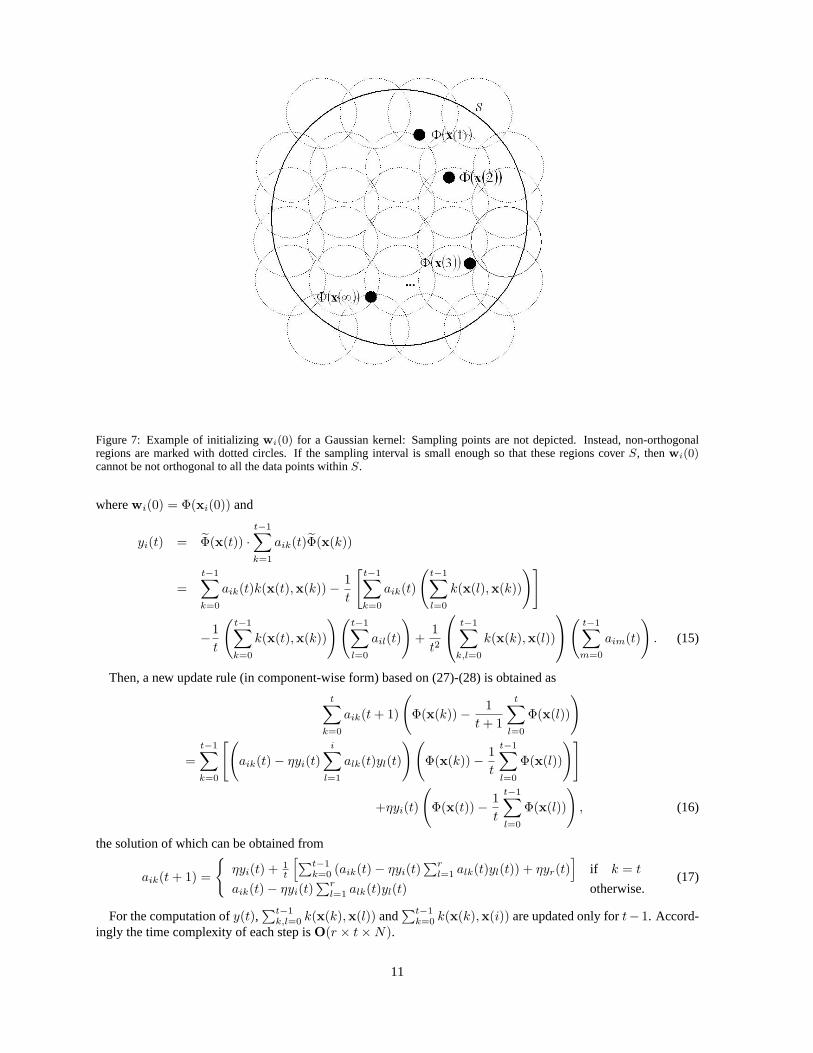
Figure 7: Example of initializingwi(0) for a Gaussian kernel: Sampling points are not depicted. Instead, non-orthogonalregions are marked with dotted circles. If the sampling interval is small enough so that these regions coverS, thenwi(0)cannot be not orthogonal to all the data points withinS.

wherewi(0) = Φ(xi(0)) and

yi(t) = Φ(x(t)) ·t−1∑k=1

aik(t)Φ(x(k))

=t−1∑k=0

aik(t)k(x(t),x(k))− 1t

[t−1∑k=0

aik(t)

(t−1∑l=0

k(x(l),x(k))

)]

−1t

(t−1∑k=0

k(x(t),x(k))

)(t−1∑l=0

ail(t)

)+

1t2

t−1∑k,l=0

k(x(k),x(l))

( t−1∑m=0

aim(t)

). (15)

Then, a new update rule (in component-wise form) based on (27)-(28) is obtained as

t∑k=0

aik(t + 1)

(Φ(x(k))− 1

t + 1

t∑l=0

Φ(x(l))

)

=t−1∑k=0

[(aik(t)− ηyi(t)

i∑l=1

alk(t)yl(t)

)(Φ(x(k))− 1

t

t−1∑l=0

Φ(x(l))

)]

+ηyi(t)

(Φ(x(t))− 1

t

t−1∑l=0

Φ(x(l))

), (16)

the solution of which can be obtained from

aik(t + 1) =

{ηyi(t) + 1

t

[∑t−1k=0 (aik(t)− ηyi(t)

∑rl=1 alk(t)yl(t)) + ηyr(t)

]if k = t

aik(t)− ηyi(t)∑r

l=1 alk(t)yl(t) otherwise.(17)

For the computation ofy(t),∑t−1

k,l=0 k(x(k),x(l)) and∑t−1

k=0 k(x(k),x(i)) are updated only fort− 1. Accord-ingly the time complexity of each step isO(r × t×N).

11

Acknowledgments. The authors greatly profited from discussions with A. Gretton, M. Hein, and G. Bakır.

References[1] B. Scholkopf, A. Smola, and K. Muller. Nonlinear component analysis as a kernel eigenvalue problem.Neural Compu-

tation, 10(5):1299–1319, 1998.

[2] B. Scholkopf and A. Smola.Learning with Kernels. MIT Press, Cambridge, MA, 2002.

[3] E. Oja. A simplified neuron model as a principal component analyzer.Journal of Mathematical Biology, 15:267–273,1982.

[4] T. D. Sanger. Optimal unsupervised learning in a single-layer linear feedforward neural netowork.Neural Networks,12:459–473, 1989.

[5] S. Mika, B. Scholkopf, A. J. Smola, K.-R. Muller, M. Scholz, and G. Ratsch. Kernel PCA and de-noising in featurespaces. In M. S. Kearns, S. A. Solla, and D. A. Cohn, editors,Advances in Neural Information Processing Systems 11,pages 536–542, Cambridge, MA, 1999. MIT Press.

[6] L. Ljung. Analysis of recursive stochastic algorithms.IEEE Trans. Automatic Control, 22(4):551–575, 1977.

[7] S. Haykin.Neural Networks: A Comprehensive Foundation. Prentice Hall, New Jersey, 2nd edition, 1999.

[8] D. J. Field. What is the goal of sensory coding?Neural Computation, 6:559–601, 1994.

[9] C. J. C. Burges. Simplified support vector decision rules. In L. Saitta, editor,Proceedings of the 13th InternationalConference on Machine Learning, pages 71–77, San Mateo, CA, 1996. Morgan Kaufmann.

[10] J. T. Kwok and I. W. Tsang. Finding the pre-images in kernel principal component analysis.6th Annual Workshop OnKernel Machines, Whistler, Canada, 2002, poster available at http://www.cs.ust.hk/∼jamesk/kernels.html.

[11] F. M. Candocia.A unified superresolution approach for optical and synthetic aperture radar images. PhD thesis, Univ.of Florida, Grainesville, 1998.

[12] A. S. Georghiades, P. N. Belhumeur, and D. J. Kriegman. From few to many: illumination cone models for face recogni-tion under variable lighting and pose.IEEE Trans. Pattern Analalysis and Machine Intelligence, 23(6):643–660, 2001.

[13] S. Mika, G. Ratsch, J. Weston, B. Scholkopf, and K.-R. Muller. Fisher discriminant analysis with kernels. In Y.-H. Hu,J. Larsen, E. Wilson, and S. Douglas, editors,Neural Networks for Signal Processing IX, pages 41–48. IEEE, 1999.

[14] J. H. van Hateren and A. van der Schaaf. Independent component filters of natural images compared with simple cells inprimary visual cortex.Proc. R. Soc. Lond. B, 265:359–366, 1997.

12