Kernel-based Collocation Methods versus Galerkin Finite ...mypages.iit.edu/~qye3/Kernel_vs_Galerkin_SPDE_FasshauerYe.pdf · Galerkin Finite Element Methods for Approximating Elliptic

Kernel-based Collocation Methods versusGalerkin Finite Element Methods forApproximating Elliptic Stochastic PartialDifferential Equations

Gregory E. Fasshauer and Qi Ye∗

Department of Applied Mathematics, Illinois Institute of Technology, Chicago,Illinois 60616 USA, [email protected] and [email protected]

Summary. We compare a kernel-based collocation method (meshfree approxima-tion method) with a Galerkin finite element method for solving elliptic stochasticpartial differential equations driven by Gaussian noise. The kernel-based collocationsolution is a linear combination of reproducing kernels obtained from related dif-ferential and boundary operators centered at chosen collocation points. Its randomcoefficients are obtained by solving a system of linear equations with multiple ran-dom right-hand sides. The finite element solution is given as a tensor product oftriangular finite elements and Lagrange polynomials defined on a finite-dimensionalprobability space. Its coefficients are obtained by solving several deterministic finiteelement problems. For the kernel-based collocation method, we directly simulate the(infinite-dimensional) Gaussian noise at the collocation points. For the finite elementmethod, however, we need to truncate the Gaussian noise into finite-dimensionalnoises. According to our numerical experiments, the finite element method has thesame convergence rate as the kernel-based collocation method provided the Gaussiannoise is truncated using a suitable number terms.

Key words: Kernel-based collocation, meshfree approximation, Galerkin fi-nite element, elliptic stochastic partial differential equations, Gaussian fields,reproducing kernel.

1 Introduction

Stochastic partial differential equations (SPDEs) form the basis of a recent,fast growing research area with many applications in physics, engineering andfinance. However, it is often difficult to obtain an explicit form of the solution.Moreover, current numerical methods usually show limited success for high-dimensional problems and in complex domains. In our recent papers [4, 11],

∗ Corresponding Author

2 G. E. Fasshauer and Q. Ye

we use a kernel-based collocation method to approximate the solution of high-dimensional SPDE problems. Since parabolic SPDEs can be transformed intoelliptic SPDEs using, e.g., an implicit time stepping scheme, solution of thelatter represents a particularly important aspect of SPDE problems.

In this paper, we compare the use of a kernel-based collocation method [4,11] (meshfree approximation method) and a Galerkin finite element method [1,2] to approximate the solution of elliptic SPDEs. For kernel-based colloca-tion, we directly simulate the Gaussian noise at a set of collocation points.For the Galerkin finite element method, on the other hand, we use a trun-cated Karhunen-Loeve expansion of the Gaussian noise in order to satisfy afinite-dimensional noise condition. For kernel-based collocation the same collo-cation locations are used to construct the deterministic basis and the randompart. For the Galerkin finite element method one needs to separately set upthe finite element basis on the spatial domain and the polynomials on theprobability space. For a given kernel function, the convergence rate of thecollocation solution depends only on the fill distance of the collocation points.The convergence rate of the finite element solution depends on the maximummesh spacing parameter and the degrees of the polynomials defined on thefinite-dimensional probability space. According to our numerical experiments,the truncation length of the Gaussian noise also affects the convergence resultsof the finite element method.

1.1 Problem Setting

Assume that D is a regular open bounded domain in Rd. Let the stochasticprocess ξ : D × Ωξ → R be Gaussian with mean zero and covariance kernelΦ : D×D → R defined on a probability space (Ωξ,Fξ,Pξ) (see Definition A.1).We consider an elliptic SPDE driven by the Gaussian noise ξ with Dirichletboundary conditions

∆u = f + ξ, in D,u = 0, on ∂D,

(1)

where ∆ is the Laplacian and f : D → R is a deterministic function. We cansolve the SPDE (1) by either of the following two numerical methods.Kernel-based collocation method (KC): We simulate the Gaussian noiseξ with covariance structure Φ(x,y) at a finite collection of predeterminedcollocation points

XD := x1, · · · ,xN ⊂ D, X∂D := xN+1, · · · ,xN+M ⊂ ∂D

and approximate u using a kernel-based collocation method written as

u(x) ≈ u(x) :=

N∑k=1

ck∆2

∗K(x,xk) +

M∑k=1

cN+k

∗K(x,xN+k), x ∈ D,

Kernel-based Collocation vs. Galerkin Finite Element for SPDEs 3

where∗K is an integral-type kernel associated with a reproducing kernel K (see

Equation (5) in Appendix Appendix A.). Here ∆2 means that we differentiate

with respect to the second argument, i.e., ∆2

∗K(x,xk) = ∆y

∗K(x,y)|y=xk .

The unknown random coefficients c := (c1, · · · , cN+M )T

are obtained by solv-ing a random system of linear equations (with constant deterministic systemmatrix and random right-hand side that varies with each realization of thenoise). Details are provided in Section 2.Galerkin finite element method (FE): Since the Galerkin finite elementmethod is based on a finite-dimensional noise assumption (see [1, 2]), assumingΦ ∈ L2(D × D), we truncate the Gaussian noise ξ by a Karhunen-Loeveexpansion, i.e.,

ξ ≈ ξn :=

n∑k=1

ζk√qkφk, and ζk ∼ i.i.d. N (0, 1), k = 1, · · · , n,

where qk and φk are eigenvalues and eigenfunctions of the covariance kernelΦ, i.e.,

∫D Φ(x,y)φk(y)dy = qkφk(x). We approximate the original SPDE (1)

by another elliptic SPDE driven by the truncated Gaussian noise ξn∆un = f + ξn, in D,un = 0, on ∂D.

(2)

Next we combine the finite element method in spatial domain D := D ∪ ∂Dand the collocation in the zeros of suitable tensor product orthogonal polyno-mials (Gaussian points) in the finite-dimensional probability space. We obtainthe approximation as a tensor product of the finite element solutions definedon the spatial domain and the Lagrange polynomials defined on the finite-dimensional probability space, i.e., uh,p ≈ un ≈ u, where h is the maximummesh spacing parameter and p = (p1, · · · , pn) is the degree of the Lagrangepolynomials. Details are provided in Section 3.

Remark 1.1. Because Φ is always positive semi-definite Mercer’s theorem en-sures that its eigenvalues q1 ≥ q2 ≥ · · · ≥ 0 and its eigenfunctions φk∞k=1

form an orthonormal base of L2(D) so that Φ(x,y) =∑∞k=1 qkφk(x)φk(y).

Therefore E ‖ξ − ξn‖2L2(D) =∑∞k=n+1 qk → 0 when n → ∞, and we can

accurately represent the infinite-dimensional noise ξ by a (potentially long)truncated Karhunen-Loeve expansion.

2 Kernel-based Collocation Method

In the papers [4, 11] we use the Gaussian fields ∆S, S with means ∆µ, µ

and covariance kernels ∆1∆2

∗K,

∗K (see Theorem A.1), respectively, to con-

struct the collocation approximation u of the solution u of SPDE (1). Here

∆1∆2

∗K(xj ,xk) = ∆x∆y

∗K(x,y)|x=xj ,y=xk .


Because of the order O(∆) = 2, we suppose that the reproducing kernelHilbert space HK(D) is embedded into the L2-based Sobolev space Hm(D)where m > 2 + d/2.

Remark 2.1. Since we want to interpolate the values of the differential equa-tion at the collocation points, ∆ω(x) needs to be well-defined pointwise foreach available solution ω ∈ HK(D) ⊆ Hm(D) ⊂ C2(D). This requires theSobolev space Hm(D) to be smooth enough. If we just need a weak solutionas for the finite element method, then the order needs to satisfy m ≥ 2 only.

Since ξ is Gaussian with a known correlation structure, we can simulatethe values of ξ at the collocation points x1, · · · ,xN , i.e.,

ξ := (ξx1 , · · · , ξxN )T ∼ N (0,Φ), where Φ := (Φ(xj ,xk))N,Nj,k=1.

Consequently, we assume that the values yjNj=1 and yN+jMj=1 defined by

yj := f(xj) + ξxj , j = 1, · · · , N, yN+j := 0, j = 1, · · · ,M,

are known. Moreover we can also obtain the joint probability density functionpy of the random vector yξ := (y1, · · · , yN+M )T .

We define the product space

ΩKξ := ΩK ×Ωξ, FKξ := FK ⊗Fξ, Pµξ := Pµ ⊗ Pξ,

where the probability measure Pµ is defined on (HK(D),B(HK(D))) =(ΩK ,FK) as in Theorem A.1, and the probability space (Ωξ,Fξ,Pξ) is givenin the SPDE (1). We assume that the random variables defined on the originalprobability spaces are extended to random variables on the new probabilityspace in the natural way: if random variables V1 : ΩK → R and V2 : Ωξ → Rare defined on (ΩK ,FK ,Pµ) and (Ωξ,Fξ,Pξ), respectively, then

V1(ω1, ω2) := V1(ω1), V2(ω1, ω2) := V2(ω2), for each ω1 ∈ ΩK and ω2 ∈ Ωξ.

Note that in this case the random variables have the same probability distri-butional properties, and they are independent on (ΩKξ,FKξ,Pµξ ). This impliesthat the stochastic processes ∆S, S and ξ can be extended to the productspace (ΩKξ,FKξ,Pµξ ) while preserving the original probability distributionalproperties, and that (∆S,S) and ξ are independent.

2.1 Approximation of SPDEs

Fix any x ∈ D. Let Ax(v) := ω1 × ω2 ∈ ΩKξ : ω1(x) = v for each v ∈ R,

andAyξPB := ω1 × ω2 ∈ ΩKξ : ∆ω1(x1) = y1(ω2), . . . , ω1(xN+M ) = yN+M (ω2).Using the methods in [4] and Theorem A.1, we obtain

Pµξ (Ax(v)|AyξPB) = Pµξ (Sx = v|SPB = yξ) = pµx(v|yξ),


where pµx(·|·) is the conditional probability density function of the random vari-able Sx given the random vector SPB := (∆Sx1

, · · · , ∆SxN , SxN+1, · · · , SxN+M

)T .(Here yξ is viewed as given values.) According to the natural extension rule,pµx is consistent with the formula (6). Then the approximation u(x) is solvedby the maximization problem

u(x) = argmaxv∈R

supµ∈HK(D)

pµx(v|yξ).

If the covariance matrix

∗KPB :=

(∆1∆2

∗K(xj ,xk))N,Nj,k=1, (∆1

∗K(xj ,xN+k))N,Mj,k=1

(∆2

∗K(xN+j ,xk))M,N

j,k=1, (∗K(xN+j ,xN+k))M,M

j,k=1

∈ R(N+M)×(N+M)

is nonsingular, then one solution of the above maximum problem has the form

u(x) :=

N∑k=1

ck∆2

∗K(x,xk)+

M∑k=1

cN+k

∗K(x,xN+k) = kPB(x)T

∗KPB

−1yξ, (3)

where kPB(x) := (∆2

∗K(x,x1), · · · , ∆2

∗K(x,xN ),

∗K(x,xN+1), · · · ,

∗K(x,xN+M ))T .

This means that its random coefficients are obtained from the linear equation

system∗KPBc = yξ.

The estimator u also satisfies the interpolation condition, i.e., ∆u(x1) =y1, . . . ,∆u(xN ) = yN and u(xN+1) = yN+1, . . . , u(xN+M ) = yN+M . It is ob-vious that u(·, ω2) ∈ HK(D) for each ω2 ∈ Ωξ. Since the random part of u(x)is only related to yξ, we can formally rewrite u(x, ω2) as u(x,yξ) and u(x) canbe transferred to a random variable defined on the finite-dimensional probabil-ity space (RN+M ,B(RN+M ), µy), where the probability measure µy is definedby µy(dv) := py(v)dv. Moreover, the probability distributional properties ofu(x) do not change when (Ωξ,Fξ,Pξ) is replaced by (RN+M ,B(RN+M ), µy).

Remark 2.2. The random coefficients are obtained solving by system of lin-ear equations that is slightly different from [4]. However the main ideas andtechniques are the same as in [4]. For this estimator it is easier to derive errorbounds and compare with Galerkin finite element method. A lot more detailsof the relationship between the two different estimators are provided in [11,Chapter 7].

2.2 Convergence Analysis

We assume that u(·, ω2) belongs to HK(D) almost surely for ω2 ∈ Ωξ. There-fore u can be seen as a map from Ωξ into HK(D). So we have u ∈ ΩKξ =ΩK ×Ωξ.

We fix any x ∈ D and any ε > 0. Let the subset


Eεx :=ω1 × ω2 ∈ ΩKξ : |ω1(x)− u(x, ω2)| ≥ ε,

such that ∆ω1(x1) = y1(ω2), . . . , ω1(xN+M ) = yN+M (ω2).

Because ∆Sx(ω1, ω2) = ∆Sx(ω1) = ∆ω1(x), Sx(ω1, ω2) = Sx(ω1) = ω1(x)and yξ(ω1, ω2) = yξ(ω2) for each ω1 ∈ ΩK and ω2 ∈ Ωξ (see Theorem A.1)we can deduce that

Pµξ (Eεx) = Pµξ(|Sx − u(x)| ≥ ε such that SPB = yξ

)=

∫RN+M

∫|v−u(x,v)|≥ε

pµx(v|v)py(v)dvdv

=

∫RN+M

erfc

(ε√

2σ(x)

)py(v)dv = erfc

(ε√

2σ(x)

),

where the variance of pµx is σ(x)2 =∗K(x,x) − kPB(x)T

∗KPB

−1kPB(x) (seeEquation (6) given in Appendix Appendix A.).

The reader may note that the form of the expression for the variance σ(x)2

is analogous to that of the power function [5, 10], and we can therefore usethe same techniques as in the proofs from [4, 5, 10, 11] to obtain a formulafor the order of σ(x), i.e.,

σ(x) = O(hm−2−d/2X ),

where hX = supx∈Dminxj∈XD∪X∂D ‖x− xj‖2 is the fill distance of X :=XD ∪X∂D. This implies that

supµ∈HK(D)

Pµξ (Eεx) = O

(hm−2−d/2X

ε

).

Because |u(x, ω2)− u(x, ω2)| ≥ ε if and only if u ∈ Eεx we conclude that

supµ∈HK(D)

Pµξ(‖u− u‖L∞(D) ≥ ε

)≤ supµ∈HK(D),x∈D

Pµξ (Eεx)→ 0, when hX → 0.

Therefore we say that the estimator u converges to the exact solution u ofthe SPDE (1) in all probabilities Pµξ when hX goes to 0.

Sometimes we know only that the solution u ∈ Hm(D). In this case, aslong as the reproducing kernel Hilbert space is dense in the Sobolev spaceHm(D) with respect to its Sobolev norm, we can still say that u converges tou in probability.

3 Galerkin Finite Element Method

The right hand side of the SPDE (2)


fξn(x, ζ) := f(x) + ξnx = f(x) +

n∑k=1

ζk√qkφk(x), x ∈ D,

and the random vector ζ := (ζ1, · · · , ζn)T has the joint standard normaldensity function

ρn(z) :=

n∏k=1

ρ(zk), z ∈ Rn, where ρ(z) :=1√2πe−z

2/2.

Therefore we can replace the probability space (Ωξ,Fξ,Pξ) by a finite-dimensional probability space (Rn,B(Rn), µζ) such that un and ξn have thesame probability distributional properties on both probability spaces, wherethe probability measure µζ is defined by µζ(dz) := ρn(z)dz.

In the paper [1] the numerical approximation uh,p of the solution un of theSPDE (2) is sought in a finite-dimensional subspace Vh,p based on a tensorproduct, Vh,p := Hh(D)⊗ Pp(Rn), where the following hold:

C1) Hh(D) ⊂ H10(D) is a standard finite element space, which contains con-

tinuous piecewise polynomials defined on regular triangulations with amaximum mesh spacing parameter h.

C2) Pp(Rn) := ⊗nk=1Ppk(R) ⊂ L2,ρn(Rn) is the span of the tensor productof polynomials with degree at most p = (p1, · · · , pn), where Ppk(R) is aspace of univariate polynomials of degree pk for each k = 1, . . . , n.

Thus the approximation uh,p ∈ Vh,p and uh,p(x) is a random variabledefined on the finite-dimensional probability space (Rn,B(Rn), µζ).

Next we construct the Gaussian points

zj := (z1,j1 , · · · , zn,jn)T , j ∈ Np := j ∈ Nn : 1 ≤ jk ≤ pk + 1, k = 1, . . . , n ,

where zk,1, . . . , zk,pk+1 are the roots of the Hermite polynomials ηpk+1 of de-gree pk + 1 for each dimension k = 1, . . . , n. The ηpk+1 are also orthogonalpolynomials on the space Ppk(R) with respect to a standard normal weight ρ.Here these Hermite polynomials are only used to set up the Gaussian pointsfor approximating the Gaussian fields.

Let a polynomial base of Pp(Rn) be

lj(z) :=

n∏k=1

lk,jk(zk), j ∈ Np,

where lk,jpk+1j=1 is the Lagrange basis of Ppk(R) for each k = 1, . . . , n, i.e.,

lk,j ∈ Ppk(R), lk,j(zk,i) = δij , i, j = 1, . . . , pk + 1,

and δij is the Kronecker symbol.For each Gaussian point zj ∈ Np, we compute the finite element solution

uh(·, zj) ∈ Hh(D) of the equation


−∫D∇uh(x, zj)∇γ(x)dx =

∫Dfξn(x, zj)γ(x)dx, for any γ ∈ Hh(D).

The approximation uh,p is the tensor product of the finite element solutionsand the Lagrange polynomials, i.e.,

uh,p(x, ζ) :=∑j∈Np

uh(x, zj)lj(ζ), x ∈ D. (4)

This indicates that uh,p is interpolating at all Gaussian points zj ∈ Np.We assume that un belongs to L2,ρn(Rn)⊗H1

0(D). According to [1, The-orem 4.1] and [1, Lemma 4.7] we get the error bound

‖Eρn(un − uh,p)‖H10(D)

≤C1 infw∈L2,ρn (Rn)⊗Hh(D)

(∫DEρn |∇un(x)−∇w(x)|2 dx

)1/2

+ C2

n∑k=1

p3/2k e−rkp

1/2k

with positive constants r1, . . . , rn and C1, C2 independent of h and p.

4 Side-by-Side Comparison of Both Methods

4.1 Differences

• Probability spaces: For kernel-based collocation (KC) we transfer theprobability space (Ωξ,Fξ,Pξ) to the tensor product probability space(ΩKξ,FKξ,Pµξ ) such that the Gaussian noise ξ has the same probabil-ity distributional properties defined on both probability spaces, while forGalerkin finite elements (FE) we approximate the Gaussian noise ξ by thetruncated Gaussian noise ξn such that limn→∞E ‖ξ − ξn‖L2(D) = 0 and ξn

has the same probability distributional properties on the probability space(Ωξ,Fξ,Pξ) and the finite-dimensional probability space (Rn,B(Rn), µζ)

• Basis functions: The bases of the KC solution u are the kernel functions

∆2

∗K and

∗K centered at the collocation points XD ⊂ D and X∂D ⊂ ∂D,

while the bases of the FE solution uh,p are the tensor products of thetriangular finite element bases defined on D and the Lagrange polynomialsdefined on (Rn,B(Rn), µζ).

• Simulation: For KC we can simulate the Gaussian noise ξ at the col-location points XD because we know its covariance kernel Φ, i.e., ξ =(ξx1 , · · · , ξxN )T ∼ N (0,Φ) and Φ = (Φ(xj ,xk))N,Nj,k=1. For FE we can sim-

ulate the random vector ζ = (ζ1, · · · , ζ2)T ∼ N (0, In) in order to introducerandom variables on (Rn,B(Rn), µζ).

• Interpolation: In KC ∆u and u are interpolating at the collocation pointsXD ∪ X∂D ⊂ D in the domain space, respectively, while in FE uh,p isinterpolating at the Gaussian points Np ⊂ Rn in the probability space.


• Function spaces: For KC, u ∈ span∆2

∗K(·,xj),

∗K(·,xN+k)N,Mj,k=1 ⊗

P1(RN+M ) ⊂ HK(D) ⊗ L2,py (RN+M ), while for FE we have uh,p ∈Hh(D)⊗ Pp(Rn) ⊂ H1

0(D)⊗ L2,ρn(Rn).• Approximation properties: The KC result u approximates the solution

u of the SPDE (1) and its convergence rate depends on the fill distance hXof the collocation points, while the FE result uh,p approximates the trun-cated solution un of the SPDE (2) with a convergence rate that dependson the maximum mesh spacing parameter h of the triangulation and thedegree p of the Lagrange polynomials.

4.2 Relationship Between the Two Methods

Roughly speaking, the random parts of u and uh,p are simulated by the normalrandom vectors ξ and ζ, respectively.

For the following we assume that Φ is positive definite on D and thedimensions of ξ and ζ are the same, i.e., N = n.

We firstly show the relationship between ξ and ζ. Since Φ is positivedefinite, we have the decomposition Φ = VDVT , where D and V are theeigenvalues and eigenvector matrices of Φ, respectively. Therefore

ξ ∼ VD1/2ζ ∼ N (0,Φ), ζ ∼ D−1/2VT ξ ∼ N (0, IN ).

We can also use ξ and ζ to approximate the Gaussian noise ξx for anyfixed x ∈ D. Using simple kriging, we let

ξx := c(x)T ξ = b(x)TΦ−1ξ ∼ N (0, b(x)TΦ−1b(x)),

where b(x) := (Φ(x,x1), · · · , Φ(x,xN ))T . According to [9],

E∣∣∣ξx − ξx∣∣∣2 = Φ(x,x)− b(x)TΦ−1b(x) = O(hkXD

),

when Φ ∈ C2k(D ×D) and hXD is the fill distance of XD. For the Karhunen-Loeve expansion,

ξNx =

N∑j=1

√qjφj(x)ζj = φ(x)TQ1/2ζ ∼ N (0,φ(x)TQφ(x)),

where φ(x) := (φ1(x), · · · , φN (x))T and Q = diag(q1, · · · , qN ). We also have

E

∫D

∣∣ξx − ξNx ∣∣2 dx =

∞∑j=N+1

qj .

This shows that the kernel-based method and the finite element method, re-spectively, use a kernel basis and a spectral basis to approximate Gaussian


fields. It also shows that we should suitably choose collocation points suchthat

limN→∞

hXD = 0 =⇒ limN→∞

ξ = limN→∞

ξN = ξ.

Usually, the smoothness of Φ is related to its eigenvalues in the sense that theorder k of continuous differentiability becomes large when the eigenvalues qjdecrease fast, e.g., Φ(x, y) =

∑∞j=1(2πj)−2k sin(2πjx) sin(2πjy).

Following these discussions, when the eigenvalues of the covariance kernelΦ decrease fast, then the Galerkin finite element method seems to be preferableto the kernel-based collocation method because we can truncate the Gaussiannoise ξ at a low dimension. However, when the eigenvalues change slowly,then we may use the kernel-based collocation method because we are able todirectly simulate ξ by its covariance structure.

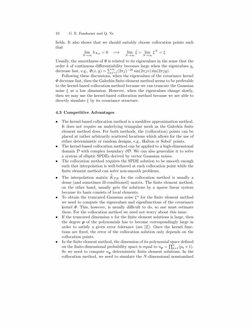
4.3 Competitive Advantages

• The kernel-based collocation method is a meshfree approximation method.It does not require an underlying triangular mesh as the Galerkin finiteelement method does. For both methods, the (collocation) points can beplaced at rather arbitrarily scattered locations which allows for the use ofeither deterministic or random designs, e.g., Halton or Sobol’ points.

• The kernel-based collocation method can be applied to a high-dimensionaldomain D with complex boundary ∂D. We can also generalize it to solvea system of elliptic SPDEs derived by vector Gaussian noises.

• The collocation method requires the SPDE solution to be smooth enoughsuch that interpolation is well-behaved at each collocation point while thefinite element method can solve non-smooth problems.

• The interpolation matrix∗KPB for the collocation method is usually a

dense (and sometimes ill-conditioned) matrix. The finite element method,on the other hand, usually gets the solutions by a sparse linear systembecause its basis consists of local elements.

• To obtain the truncated Gaussian noise ξn for the finite element methodwe need to compute the eigenvalues and eigenfunctions of the covariancekernel Φ. This, however, is usually difficult to do, so one must estimatethem. For the collocation method we need not worry about this issue.

• If the truncated dimension n for the finite element solutions is large, thenthe degree p of the polynomials has to become correspondingly large inorder to satisfy a given error tolerance (see [2]). Once the kernel func-tions are fixed, the error of the collocation solution only depends on thecollocation points.

• In the finite element method, the dimension of its polynomial space definedon the finite-dimensional probability space is equal to np =

∏nk=1(pk + 1).

So we need to compute np deterministic finite element solutions. In thecollocation method, we need to simulate the N -dimensional nonstandard


normal vector. Therefore, when n N we may choose the finite elementmethod, while vice versa the collocation method may be preferable.

• For various covariance kernels Φ for the Gaussian noise ξ, the choice ofreproducing kernels can affect the kernel-based collocation solution. Howto choose the “best” kernels is still an open question. Polynomials areused to construct the approximations for the finite element method, andwe only need to determine the appropriate polynomial degree.

• The paper [1] also discusses any other tensor-product finite dimensionalnoise. In the papers [4, 11] we only consider Gaussian noises. However, onemay generalize the kernel-based collocation idea to other problems withcolored noise.

• The finite element method works for any elliptic SPDE whose differentialoperator contains stochastic coefficients defined on a finite dimensionalprobability space. For the collocation method this idea requires furtherstudy.

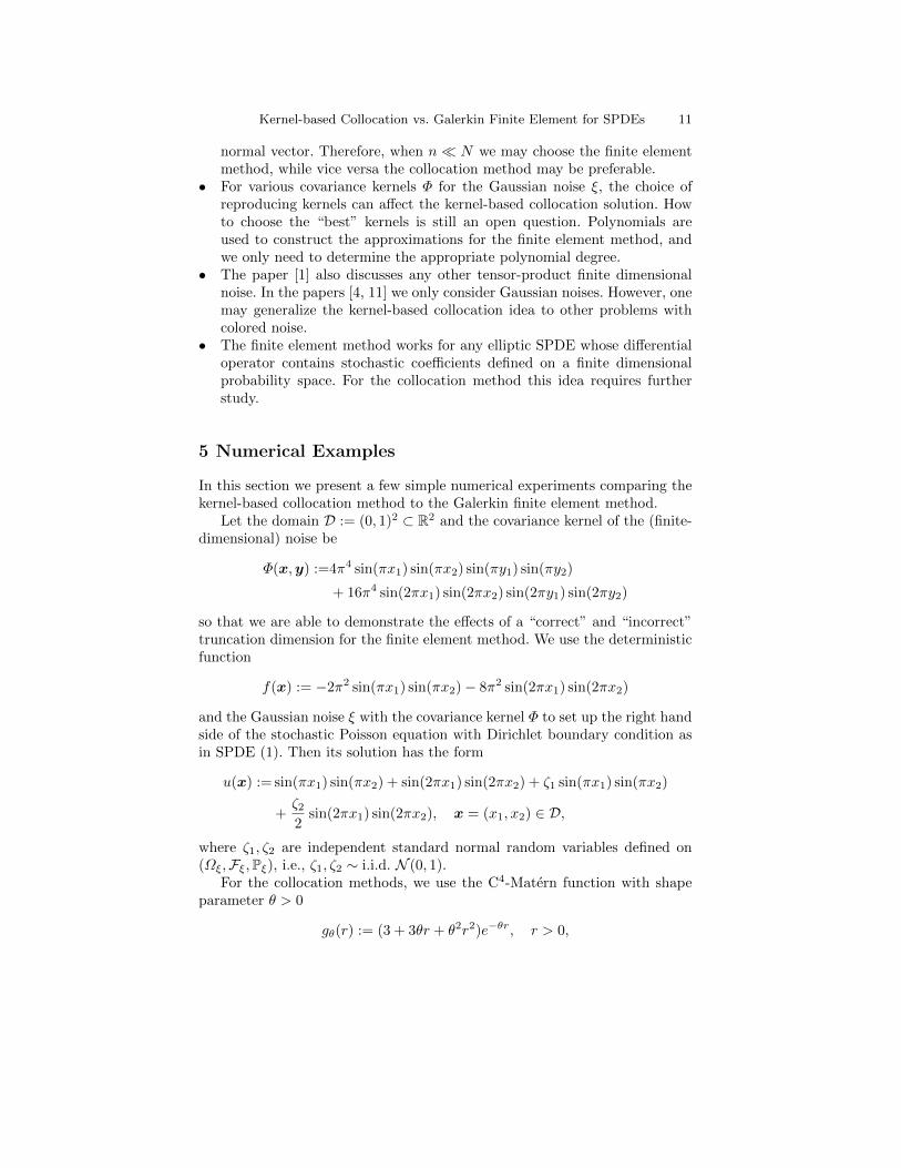
5 Numerical Examples

In this section we present a few simple numerical experiments comparing thekernel-based collocation method to the Galerkin finite element method.

Let the domain D := (0, 1)2 ⊂ R2 and the covariance kernel of the (finite-dimensional) noise be

Φ(x,y) :=4π4 sin(πx1) sin(πx2) sin(πy1) sin(πy2)

+ 16π4 sin(2πx1) sin(2πx2) sin(2πy1) sin(2πy2)

so that we are able to demonstrate the effects of a “correct” and “incorrect”truncation dimension for the finite element method. We use the deterministicfunction

f(x) := −2π2 sin(πx1) sin(πx2)− 8π2 sin(2πx1) sin(2πx2)

and the Gaussian noise ξ with the covariance kernel Φ to set up the right handside of the stochastic Poisson equation with Dirichlet boundary condition asin SPDE (1). Then its solution has the form

u(x) := sin(πx1) sin(πx2) + sin(2πx1) sin(2πx2) + ζ1 sin(πx1) sin(πx2)

+ζ22

sin(2πx1) sin(2πx2), x = (x1, x2) ∈ D,

where ζ1, ζ2 are independent standard normal random variables defined on(Ωξ,Fξ,Pξ), i.e., ζ1, ζ2 ∼ i.i.d. N (0, 1).

For the collocation methods, we use the C4-Matern function with shapeparameter θ > 0

gθ(r) := (3 + 3θr + θ2r2)e−θr, r > 0,


to construct the reproducing kernel (Sobolev-spline kernel)

Kθ(x,y) := gθ(‖x− y‖2), x,y ∈ D.

According to [6], we can deduce that its reproducing kernel Hilbert spaceHK(D) is equivalent to the L2-based Sobolev spaceH3+1/2(D) ⊂ C2(D). Then

we can compute the integral-type∗Kθ(x,y) =

∫ 1

0

∫ 1

0Kθ(x, z)Kθ(y, z)dz1dz2.

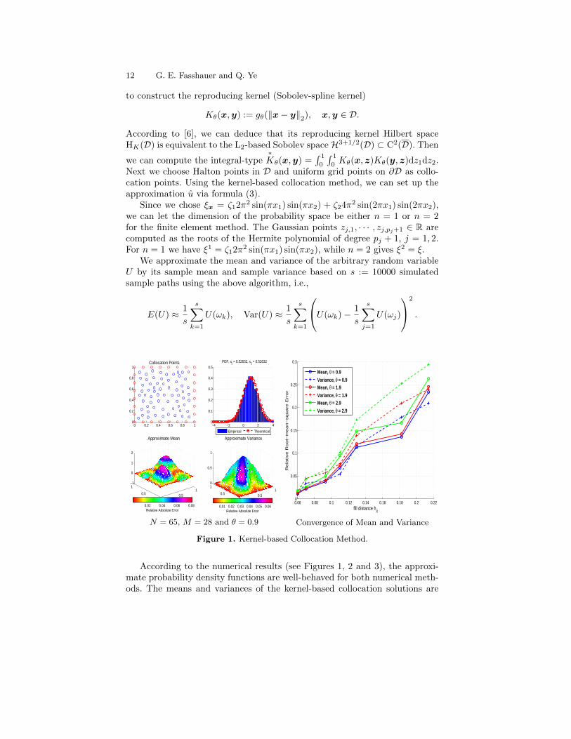
Next we choose Halton points in D and uniform grid points on ∂D as collo-cation points. Using the kernel-based collocation method, we can set up theapproximation u via formula (3).

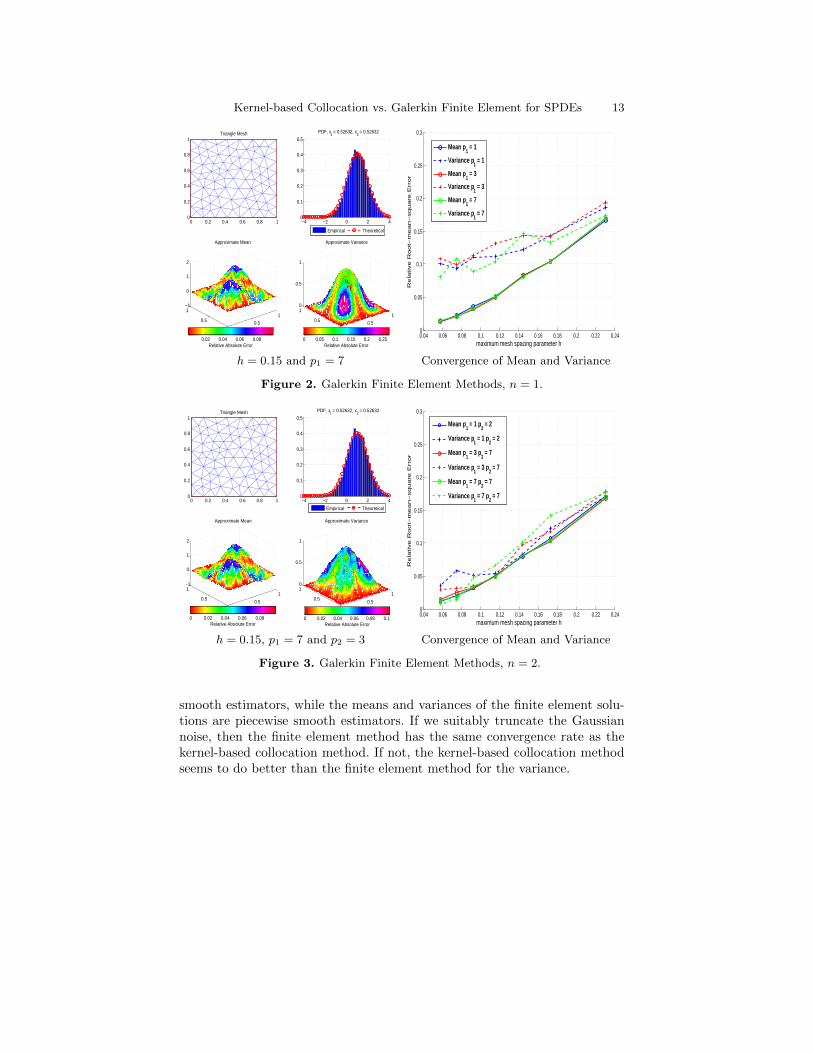
Since we chose ξx = ζ12π2 sin(πx1) sin(πx2) + ζ24π2 sin(2πx1) sin(2πx2),we can let the dimension of the probability space be either n = 1 or n = 2for the finite element method. The Gaussian points zj,1, · · · , zj,pj+1 ∈ R arecomputed as the roots of the Hermite polynomial of degree pj + 1, j = 1, 2.For n = 1 we have ξ1 = ζ12π2 sin(πx1) sin(πx2), while n = 2 gives ξ2 = ξ.

We approximate the mean and variance of the arbitrary random variableU by its sample mean and sample variance based on s := 10000 simulatedsample paths using the above algorithm, i.e.,

E(U) ≈ 1

s

s∑k=1

U(ωk), Var(U) ≈ 1

s

s∑k=1

U(ωk)− 1

s

s∑j=1

U(ωj)

2

.

00.5

1

0

0.5

1−1

0

1

2

Approximate Mean

Relative Absolute Error0.02 0.04 0.06 0.08

00.5

1

0

0.5

10

0.5

1

Approximate Variance

Relative Absolute Error0.01 0.02 0.03 0.04 0.05 0.06

−4 −2 0 2 40

0.1

0.2

0.3

0.4

0.5

PDF, x1 = 0.52632, x2 = 0.52632

Empirical Theoretical

0 0.2 0.4 0.6 0.8 10

0.2

0.4

0.6

0.8

1Collocation Points

N = 65, M = 28 and θ = 0.9

0.06 0.08 0.1 0.12 0.14 0.16 0.18 0.2 0.220

0.05

0.1

0.15

0.2

0.25

0.3

fill distance hX

Re

lative

Ro

ot−

me

an

−sq

ua

re E

rro

r

Mean, θ = 0.9

Variance, θ = 0.9Mean, θ = 1.9

Variance, θ = 1.9Mean, θ = 2.9

Variance, θ = 2.9

Convergence of Mean and Variance

Figure 1. Kernel-based Collocation Method.

According to the numerical results (see Figures 1, 2 and 3), the approxi-mate probability density functions are well-behaved for both numerical meth-ods. The means and variances of the kernel-based collocation solutions are


0 0.2 0.4 0.6 0.8 10

0.2

0.4

0.6

0.8

1Triangle Mesh

0

0.5

1

0

0.5

1−1

0

1

2

Approximate Mean

Relative Absolute Error0.02 0.04 0.06 0.08

0

0.5

1

0

0.5

10

0.5

1


Relative Absolute Error0 0.05 0.1 0.15 0.2 0.25

−4 −2 0 2 40

0.1

0.2

0.3

0.4

0.5

PDF, x1 = 0.52632, x2 = 0.52632


h = 0.15 and p1 = 7

0.04 0.06 0.08 0.1 0.12 0.14 0.16 0.18 0.2 0.22 0.240

0.05

0.1

0.15

0.2

0.25

0.3

maximum mesh spacing parameter h

Re

lative

Ro

ot−

me

an

−sq

ua

re E

rro

r

Mean p1 = 1

Variance p1 = 1

Mean p1 = 3

Variance p1 = 3

Mean p1 = 7

Variance p1 = 7


Figure 2. Galerkin Finite Element Methods, n = 1.

0 0.2 0.4 0.6 0.8 10

0.2

0.4

0.6

0.8

1Triangle Mesh

0

0.5

1

0

0.5

1−1

0

1

2

Approximate Mean

Relative Absolute Error0 0.02 0.04 0.06 0.08

0

0.5

1

0

0.5

10

0.5

1


Relative Absolute Error0 0.02 0.04 0.06 0.08 0.1

−4 −2 0 2 40

0.1

0.2

0.3

0.4

0.5

PDF, x1 = 0.52632, x2 = 0.52632


h = 0.15, p1 = 7 and p2 = 3

0.04 0.06 0.08 0.1 0.12 0.14 0.16 0.18 0.2 0.22 0.240

0.05

0.1

0.15

0.2

0.25

0.3

maximum mesh spacing parameter h

Re

lative

Ro

ot−

me

an

−sq

ua

re E

rro

r

Mean p1 = 1 p

2 = 2

Variance p1 = 1 p

2 = 2

Mean p1 = 3 p

2 = 7

Variance p1 = 3 p

2 = 7

Mean p1 = 7 p

2 = 7

Variance p1 = 7 p

2 = 7


Figure 3. Galerkin Finite Element Methods, n = 2.

smooth estimators, while the means and variances of the finite element solu-tions are piecewise smooth estimators. If we suitably truncate the Gaussiannoise, then the finite element method has the same convergence rate as thekernel-based collocation method. If not, the kernel-based collocation methodseems to do better than the finite element method for the variance.


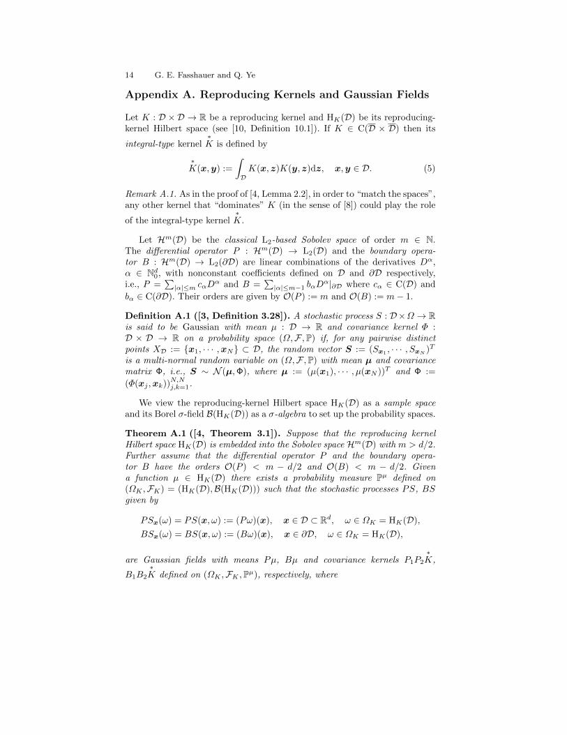
Appendix A. Reproducing Kernels and Gaussian Fields

Let K : D × D → R be a reproducing kernel and HK(D) be its reproducing-kernel Hilbert space (see [10, Definition 10.1]). If K ∈ C(D × D) then its

integral-type kernel∗K is defined by

∗K(x,y) :=

∫DK(x, z)K(y, z)dz, x,y ∈ D. (5)

Remark A.1. As in the proof of [4, Lemma 2.2], in order to “match the spaces”,any other kernel that “dominates” K (in the sense of [8]) could play the role

of the integral-type kernel∗K.

Let Hm(D) be the classical L2-based Sobolev space of order m ∈ N.The differential operator P : Hm(D) → L2(D) and the boundary opera-tor B : Hm(D) → L2(∂D) are linear combinations of the derivatives Dα,α ∈ Nd0, with nonconstant coefficients defined on D and ∂D respectively,i.e., P =

∑|α|≤m cαD

α and B =∑|α|≤m−1 bαD

α|∂D where cα ∈ C(D) and

bα ∈ C(∂D). Their orders are given by O(P ) := m and O(B) := m− 1.

Definition A.1 ([3, Definition 3.28]). A stochastic process S : D×Ω → Ris said to be Gaussian with mean µ : D → R and covariance kernel Φ :D × D → R on a probability space (Ω,F ,P) if, for any pairwise distinctpoints XD := x1, · · · ,xN ⊂ D, the random vector S := (Sx1 , · · · , SxN )T

is a multi-normal random variable on (Ω,F ,P) with mean µ and covariancematrix Φ, i.e., S ∼ N (µ,Φ), where µ := (µ(x1), · · · , µ(xN ))T and Φ :=

(Φ(xj ,xk))N,Nj,k=1.

We view the reproducing-kernel Hilbert space HK(D) as a sample spaceand its Borel σ-field B(HK(D)) as a σ-algebra to set up the probability spaces.

Theorem A.1 ([4, Theorem 3.1]). Suppose that the reproducing kernelHilbert space HK(D) is embedded into the Sobolev space Hm(D) with m > d/2.Further assume that the differential operator P and the boundary opera-tor B have the orders O(P ) < m − d/2 and O(B) < m − d/2. Givena function µ ∈ HK(D) there exists a probability measure Pµ defined on(ΩK ,FK) = (HK(D),B(HK(D))) such that the stochastic processes PS, BSgiven by

PSx(ω) = PS(x, ω) := (Pω)(x), x ∈ D ⊂ Rd, ω ∈ ΩK = HK(D),

BSx(ω) = BS(x, ω) := (Bω)(x), x ∈ ∂D, ω ∈ ΩK = HK(D),

are Gaussian fields with means Pµ, Bµ and covariance kernels P1P2

∗K,

B1B2

∗K defined on (ΩK ,FK ,Pµ), respectively, where


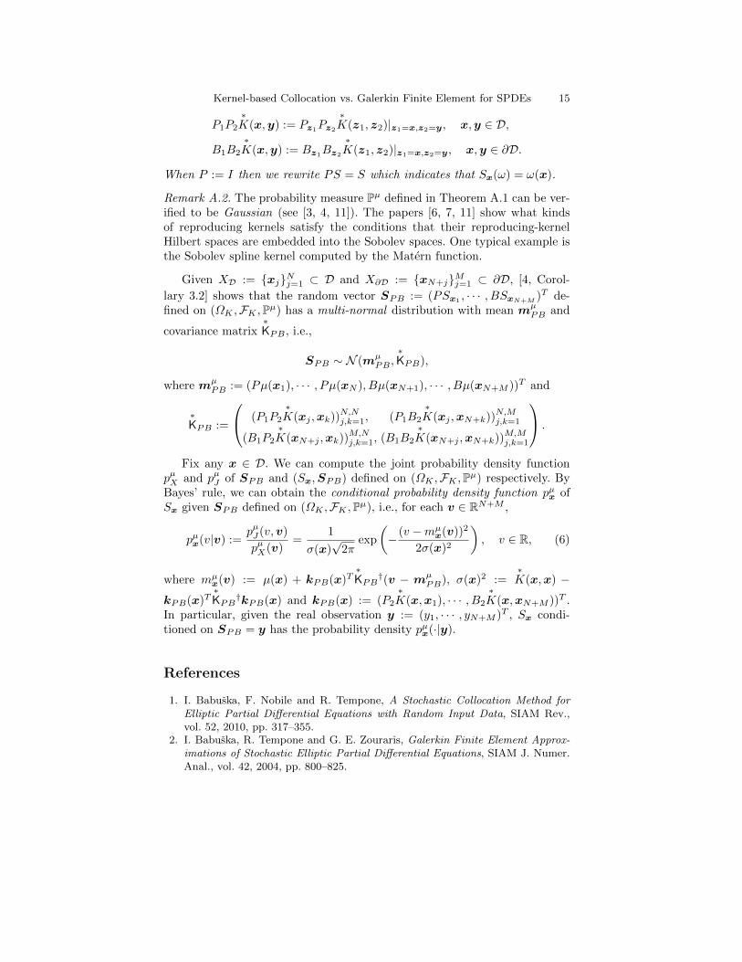
P1P2

∗K(x,y) := Pz1

Pz2

∗K(z1, z2)|z1=x,z2=y, x,y ∈ D,

B1B2

∗K(x,y) := Bz1

Bz2

∗K(z1, z2)|z1=x,z2=y, x,y ∈ ∂D.

When P := I then we rewrite PS = S which indicates that Sx(ω) = ω(x).

Remark A.2. The probability measure Pµ defined in Theorem A.1 can be ver-ified to be Gaussian (see [3, 4, 11]). The papers [6, 7, 11] show what kindsof reproducing kernels satisfy the conditions that their reproducing-kernelHilbert spaces are embedded into the Sobolev spaces. One typical example isthe Sobolev spline kernel computed by the Matern function.

Given XD := xjNj=1 ⊂ D and X∂D := xN+jMj=1 ⊂ ∂D, [4, Corol-

lary 3.2] shows that the random vector SPB := (PSx1, · · · , BSxN+M

)T de-fined on (ΩK ,FK ,Pµ) has a multi-normal distribution with mean mµ

PB and

covariance matrix∗KPB , i.e.,

SPB ∼ N (mµPB ,

∗KPB),

where mµPB := (Pµ(x1), · · · , Pµ(xN ), Bµ(xN+1), · · · , Bµ(xN+M ))T and

∗KPB :=

(P1P2

∗K(xj ,xk))N,Nj,k=1, (P1B2

∗K(xj ,xN+k))N,Mj,k=1

(B1P2

∗K(xN+j ,xk))M,N

j,k=1, (B1B2

∗K(xN+j ,xN+k))M,M

j,k=1

.

Fix any x ∈ D. We can compute the joint probability density functionpµX and pµJ of SPB and (Sx,SPB) defined on (ΩK ,FK ,Pµ) respectively. ByBayes’ rule, we can obtain the conditional probability density function pµx ofSx given SPB defined on (ΩK ,FK ,Pµ), i.e., for each v ∈ RN+M ,

pµx(v|v) :=pµJ(v,v)

pµX(v)=

1

σ(x)√

2πexp

(− (v −mµ

x(v))2

2σ(x)2

), v ∈ R, (6)

where mµx(v) := µ(x) + kPB(x)T

∗KPB

†(v − mµPB), σ(x)2 :=

∗K(x,x) −

kPB(x)T∗KPB

†kPB(x) and kPB(x) := (P2

∗K(x,x1), · · · , B2

∗K(x,xN+M ))T .

In particular, given the real observation y := (y1, · · · , yN+M )T , Sx condi-tioned on SPB = y has the probability density pµx(·|y).

References

1. I. Babuska, F. Nobile and R. Tempone, A Stochastic Collocation Method forElliptic Partial Differential Equations with Random Input Data, SIAM Rev.,vol. 52, 2010, pp. 317–355.

2. I. Babuska, R. Tempone and G. E. Zouraris, Galerkin Finite Element Approx-imations of Stochastic Elliptic Partial Differential Equations, SIAM J. Numer.Anal., vol. 42, 2004, pp. 800–825.


3. A. Berlinet and C. Thomas-Agnan, Reproducing Kernel Hilbert Spaces in Prob-ability and Statistics, Kluwer Academic Publishers, 2004.

4. I. Cialenco, G. E. Fasshauer and Q. Ye, Approximation of Stochastic PartialDifferential Equations by a Kernel-based Collocation Method, Int. J. Comput.Math., Special Issue: Recent Advances on the Numerical Solutions of StochasticPartial Differential Equations, 2012, to appear.

5. G. E. Fasshauer, Meshfree Approximation Methods with Matlab, World Scien-tific Publishing Co. Pte. Ltd., 2007.

6. G. E. Fasshauer and Q. Ye, Reproducing Kernels of Generalized Sobolev Spacesvia a Green Function Approach with Distributional Operators, Numer. Math.,vol. 119, 2011, pp. 585–611.

7. G. E. Fasshauer and Q. Ye, Reproducing Kernels of Sobolev Spaces via a GreenKernel Approach with Differential Operators and Boundary Operators, Adv.Comput. Math., DOI: 10.1007/s10444-011-9264-6.

8. M. N. Lukic and J. H. Beder, Stochastic Processes with Sample Paths in Repro-ducing Kernel Hilbert Spaces, Trans. Amer. Math. Soc., vol. 353, 2001, pp. 3945–3969.

9. M. Scheuerer, R. Schaback and M. Schlather, Interpolation of Spatial Data – AStochastic or A Deterministic Problem?, Data Page of R. Schaback’s ResearchGroup, 2010.

10. H. Wendland, Scattered Data Approximation, Cambridge University Press, 2005.11. Q. Ye, Analyzing Reproducing Kernel Approximation Methods via A Green

Function Approach, Ph.D. thesis, Illinois Institute of Technology, 2012.

Documents

Kernel-based Collocation Methods versus Galerkin Finite ...mypages.iit.edu/~qye3/Kernel_vs_Galerkin_SPDE_FasshauerYe.pdf · Galerkin Finite Element Methods for Approximating Elliptic