K&W 23 - 1

Keppel, G. & Wickens, T. D. Design and Analysis Chapter 23: Within-Subject and Mixed Designs

23.1 Varieties of Three-Factor Designs • Basically, we’re talking about three kinds of three-factor designs involving repeated measures: AxBxCxS, Ax(BxCxS), AxBx(CxS). That is, we will be considering a completely repeated measures three-factor design, a mixed design with one between factor and two repeated factors, and a mixed design with two between factors and one repeated factor. • The general approach to analyzing all of these designs is conceptually equivalent to the approach illustrated for a three-way between design. The differences emerge only in the way you’ll tell SPSS to analyze the data (and the resultant changes in the error terms used). 23.2 The Overall Analysis • The effects for any three-factor design are the same (A, B, C, AxB, AxC, BxC, AxBxC). However, as K&W illustrate in Table 23.2, the error terms appropriate for each effect do vary. You should have a sense of the source of these error terms, but realize that SPSS should compute the appropriate error terms for the overall ANOVA if you specify the design properly. The tricky part is determining error terms for post hoc analyses. J • The approach to interpreting the results of any three-factor design is the same, so the discussion of the three-way independent groups design applies here as well. That is, if the three-way interaction is significant, you should focus on interpreting that effect. If the three-way interaction is not significant, then you would focus your attention on the two-way interactions. If no interaction is significant, then you would focus your attention on the main effects. 23.3 Examples of Designs AND 23.4-5 Analytical Analyses

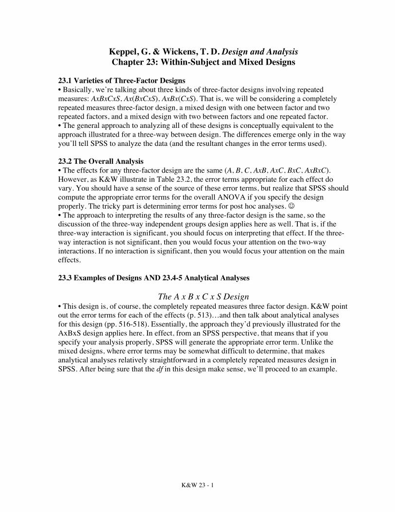
The A x B x C x S Design • This design is, of course, the completely repeated measures three factor design. K&W point out the error terms for each of the effects (p. 513)…and then talk about analytical analyses for this design (pp. 516-518). Essentially, the approach they’d previously illustrated for the AxBxS design applies here. In effect, from an SPSS perspective, that means that if you specify your analysis properly, SPSS will generate the appropriate error term. Unlike the mixed designs, where error terms may be somewhat difficult to determine, that makes analytical analyses relatively straightforward in a completely repeated measures design in SPSS. After being sure that the df in this design make sense, we’ll proceed to an example.

K&W 23 - 2

Suppose that you were conducting a 2x3x4 completely within design. Given counterbalancing issues, how many participants would you need? Suppose that you decided to use 24 participants. What df would you find in your source table?

Source df Subject A Error for A (AxS) B Error for B (BxS) C Error for C (CxS) AxB Error for AxB (AxBxS) AxC Error for AxC (AxCxS) BxC Error for BxC (BxCxS) AxBxC Error for AxBxC (AxBxCxS) Total

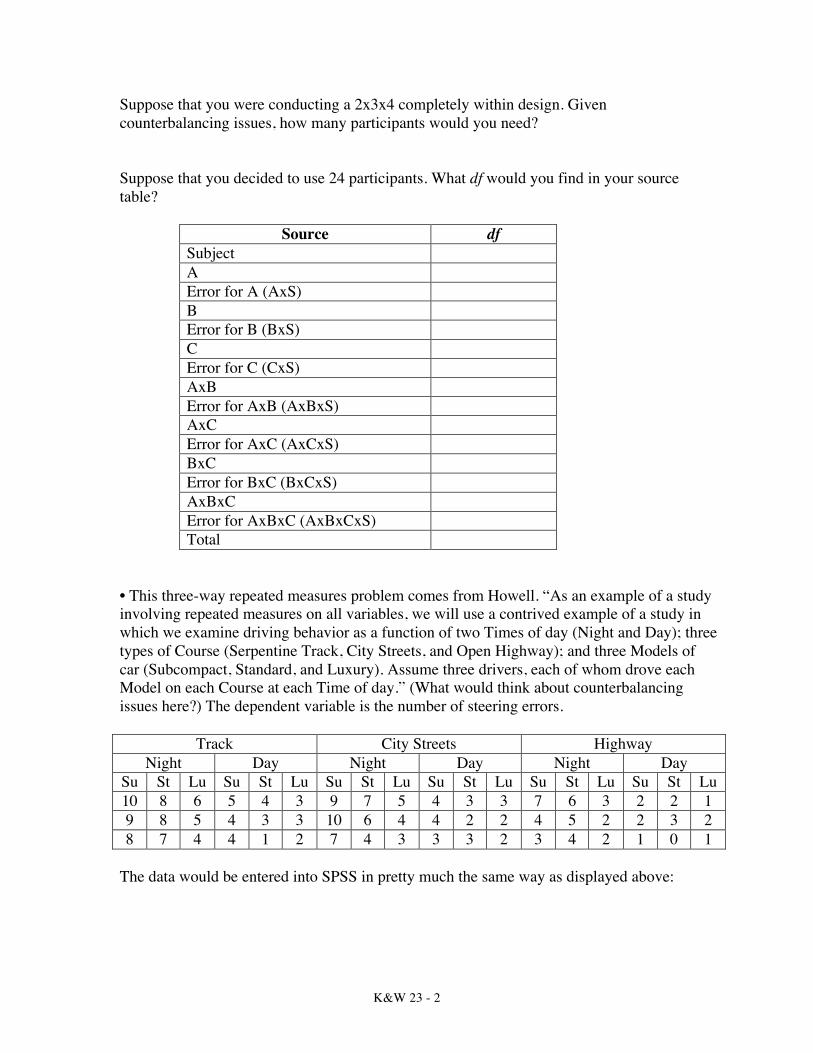
• This three-way repeated measures problem comes from Howell. “As an example of a study involving repeated measures on all variables, we will use a contrived example of a study in which we examine driving behavior as a function of two Times of day (Night and Day); three types of Course (Serpentine Track, City Streets, and Open Highway); and three Models of car (Subcompact, Standard, and Luxury). Assume three drivers, each of whom drove each Model on each Course at each Time of day.” (What would think about counterbalancing issues here?) The dependent variable is the number of steering errors.

Track City Streets Highway Night Day Night Day Night Day

Su St Lu Su St Lu Su St Lu Su St Lu Su St Lu Su St Lu 10 8 6 5 4 3 9 7 5 4 3 3 7 6 3 2 2 1 9 8 5 4 3 3 10 6 4 4 2 2 4 5 2 2 3 2 8 7 4 4 1 2 7 4 3 3 3 2 3 4 2 1 0 1

The data would be entered into SPSS in pretty much the same way as displayed above:

K&W 23 - 3

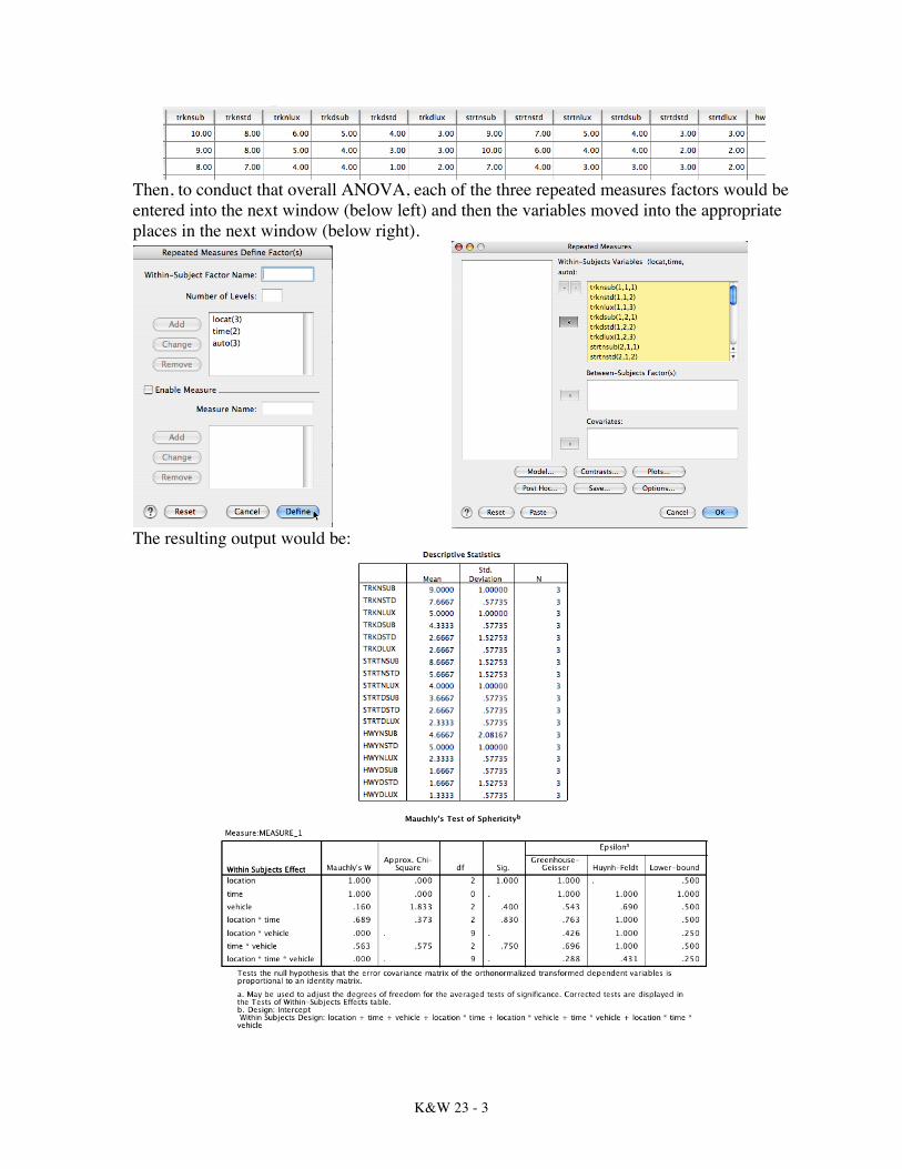
Then, to conduct that overall ANOVA, each of the three repeated measures factors would be entered into the next window (below left) and then the variables moved into the appropriate places in the next window (below right).

The resulting output would be:

K&W 23 - 4

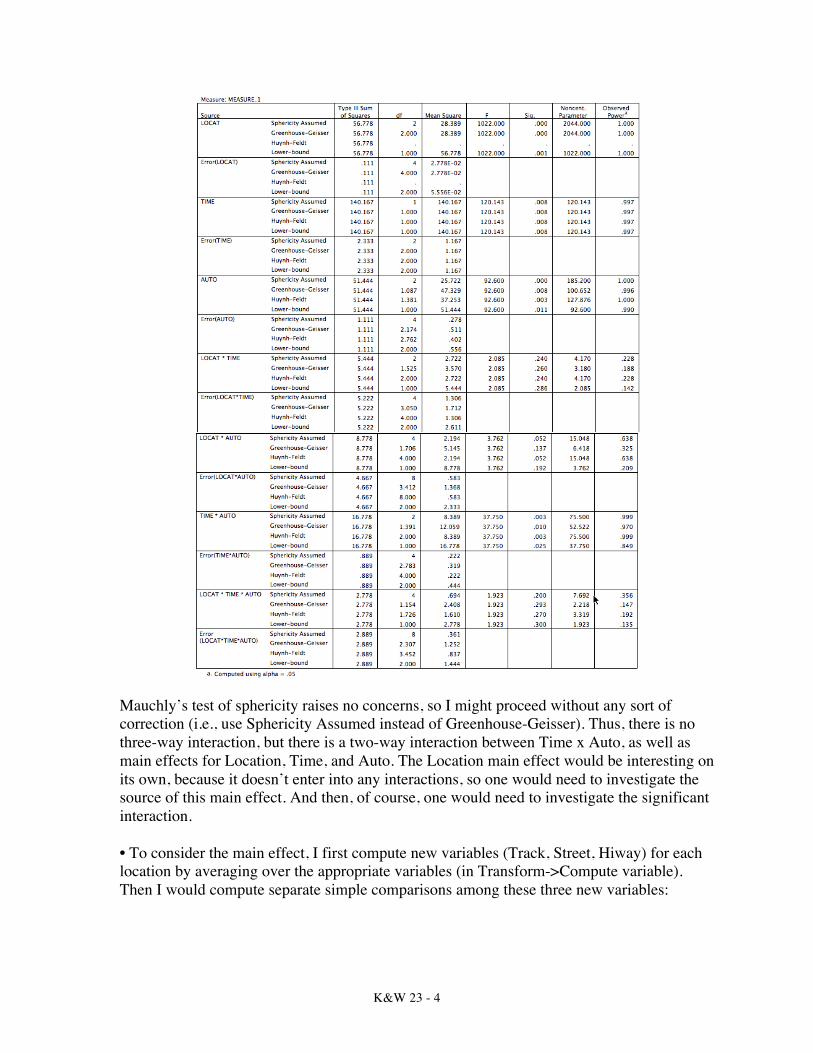
Mauchly’s test of sphericity raises no concerns, so I might proceed without any sort of correction (i.e., use Sphericity Assumed instead of Greenhouse-Geisser). Thus, there is no three-way interaction, but there is a two-way interaction between Time x Auto, as well as main effects for Location, Time, and Auto. The Location main effect would be interesting on its own, because it doesn’t enter into any interactions, so one would need to investigate the source of this main effect. And then, of course, one would need to investigate the significant interaction. • To consider the main effect, I first compute new variables (Track, Street, Hiway) for each location by averaging over the appropriate variables (in Transform->Compute variable). Then I would compute separate simple comparisons among these three new variables:

K&W 23 - 5

Thus, one could safely conclude that these drivers made significantly more errors on the track (M = 5.22) than on the street (M = 4.50) or the highway (M = 2.78), and more errors on the street than on the highway. However, if one wanted a somewhat conservative test, with three tests, the Sidák-Bonferroni procedure critical p-value would be .01695. Again, all three comparisons produced p values much less than .01695. • Alternatively, one might have SPSS compute a test of the main effect using the Sidák-Bonferroni test under Options, which would yield the same decision (all three conditions differ):

K&W 23 - 6

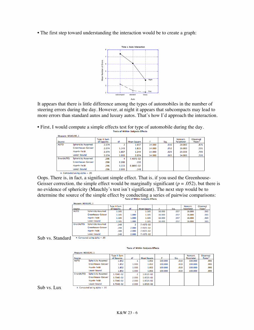
• The first step toward understanding the interaction would be to create a graph:

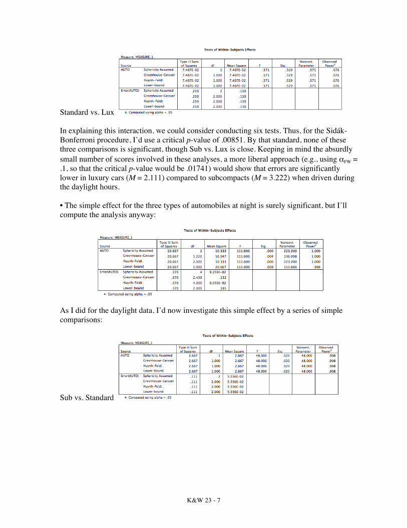
It appears that there is little difference among the types of automobiles in the number of steering errors during the day. However, at night it appears that subcompacts may lead to more errors than standard autos and luxury autos. That’s how I’d approach the interaction. • First, I would compute a simple effects test for type of automobile during the day.

Oops. There is, in fact, a significant simple effect. That is, if you used the Greenhouse-Geisser correction, the simple effect would be marginally significant (p = .052), but there is no evidence of sphericity (Mauchly’s test isn’t significant). The next step would be to determine the source of the simple effect by conducting a series of pairwise comparisons:

Sub vs. Standard

Sub vs. Lux

2

3

4

5

6

7

8

subcompact standard luxury

Time x Auto Interaction

Mea

n N

umbe

r of E

rrors

Auto

Night

Day

K&W 23 - 7

Standard vs. Lux In explaining this interaction, we could consider conducting six tests. Thus, for the Sidák-Bonferroni procedure, I’d use a critical p-value of .00851. By that standard, none of these three comparisons is significant, though Sub vs. Lux is close. Keeping in mind the absurdly small number of scores involved in these analyses, a more liberal approach (e.g., using αFW = .1, so that the critical p-value would be .01741) would show that errors are significantly lower in luxury cars (M = 2.111) compared to subcompacts (M = 3.222) when driven during the daylight hours. • The simple effect for the three types of automobiles at night is surely significant, but I’ll compute the analysis anyway:

As I did for the daylight data, I’d now investigate this simple effect by a series of simple comparisons:

Sub vs. Standard

K&W 23 - 8

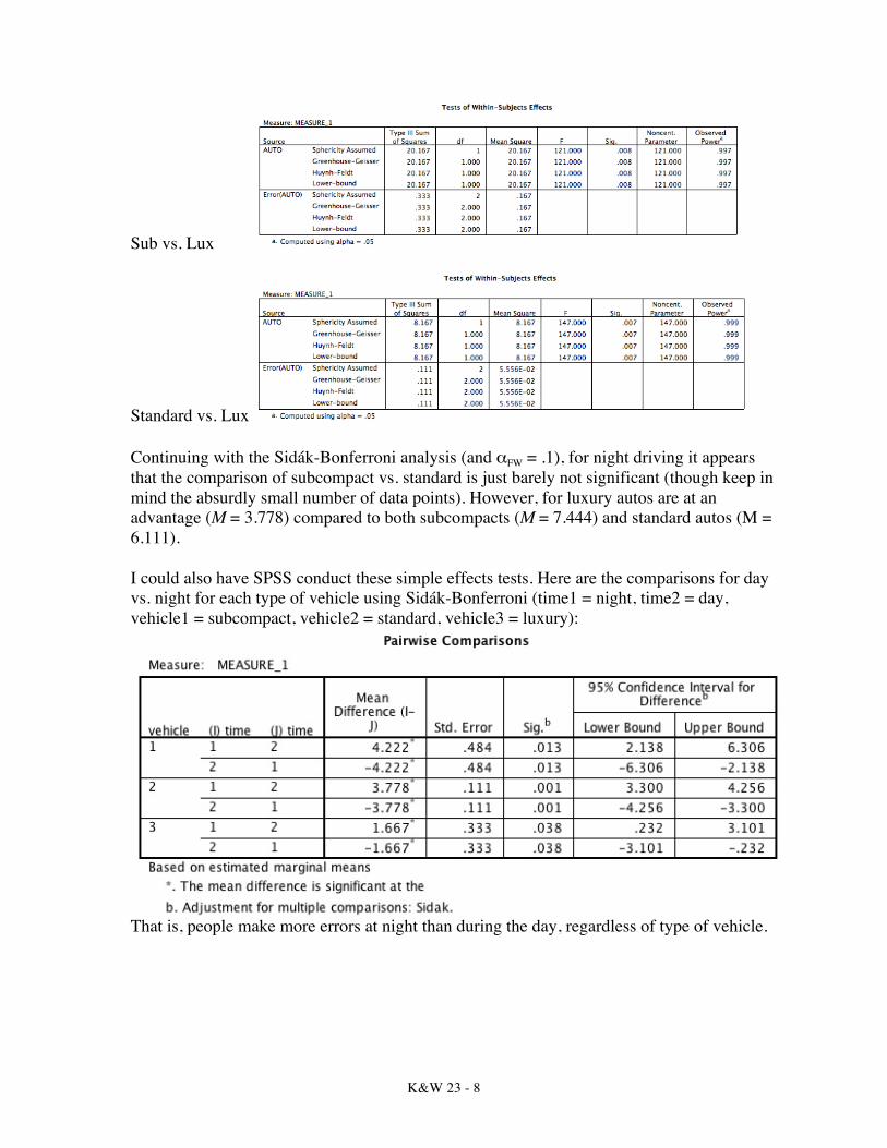
Sub vs. Lux

Standard vs. Lux Continuing with the Sidák-Bonferroni analysis (and αFW = .1), for night driving it appears that the comparison of subcompact vs. standard is just barely not significant (though keep in mind the absurdly small number of data points). However, for luxury autos are at an advantage (M = 3.778) compared to both subcompacts (M = 7.444) and standard autos (M = 6.111). I could also have SPSS conduct these simple effects tests. Here are the comparisons for day vs. night for each type of vehicle using Sidák-Bonferroni (time1 = night, time2 = day, vehicle1 = subcompact, vehicle2 = standard, vehicle3 = luxury):

That is, people make more errors at night than during the day, regardless of type of vehicle.

K&W 23 - 9

Here are the comparisons for type of vehicle at day vs. night using Sidák-Bonferroni:

Consistent with the earlier analyses, at night lux < std & sub (and std = sub). However, during day only lux < sub. • Results There was a significant main effect for location of the driving task, F(2,4) = 1022.0, MSE = .028, p < .001, η2 = .998. Post hoc tests using the Sidák-Bonferroni procedure demonstrated that there were significantly more steering errors on the track (M = 5.22) than on the street (M = 4.50) or the highway (M = 2.78), and more errors on the street than on the highway. (Maybe drivers are more foolhardy when on a track? Or maybe the track is a trickier path to drive on?) There was a main effect for time of day, F(1,2) = 120.143, MSE = 1.167, p < .001, η2 = .984. There was also a main effect for type of vehicle driven, F(2,4) = 92.6, MSE = .278, p < .001, η2 = .979. The three-way interaction among location, time of day, and type of vehicle was not significant, F(4,8) = 1.923, MSE = .361, p = .20, η2 = .49. Nor were the interactions between location and time [F(2,4) = 2.085, MSE = 1.306, p = .240, η2 = .51] and location and vehicle [F(4,8) = 3.762, MSE = .583, p = .052, η2 = .653]. However, there was an interaction between time of day and type of vehicle, F(2,4) = 37.75, MSE = .222, p = .003, η2 = .95. Post hoc tests using the Sidák-Bonferroni procedure demonstrated that under daylight driving conditions steering errors are significantly lower in luxury cars (M = 2.111) compared to subcompacts (M = 3.222). However, under night driving conditions luxury autos are at an advantage (M = 3.778) compared to both subcompacts (M = 7.444) and standard autos (M = 6.111). [I would likely refer the reader to a figure, rather than reporting all the means.]

K&W 23 - 10

The A x B x (C x S) Design

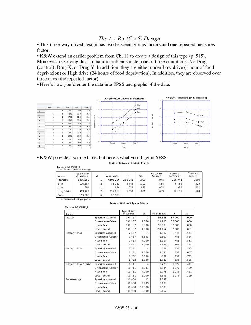
• This three-way mixed design has two between groups factors and one repeated measures factor. • K&W extend an earlier problem from Ch. 11 to create a design of this type (p. 515). Monkeys are solving discrimination problems under one of three conditions: No Drug (control), Drug X, or Drug Y. In addition, they are either under Low drive (1 hour of food deprivation) or High drive (24 hours of food deprivation). In addition, they are observed over three days (the repeated factor). • Here’s how you’d enter the data into SPSS and graphs of the data:

• K&W provide a source table, but here’s what you’d get in SPSS:

0

5

10

15

20

25

Control Drug X Drug Y

KW.p515.Low Drive (1 hr deprived)

Num

ber o

f Erro

rs

Drug

Day1

Day2

Day3

0

5

10

15

20

25

Control Drug X Drug Y

KW.p515.High Drive (24 hr deprived)

Num

ber o

f Erro

rs

Drug

Day1

Day2

Day3

K&W 23 - 11

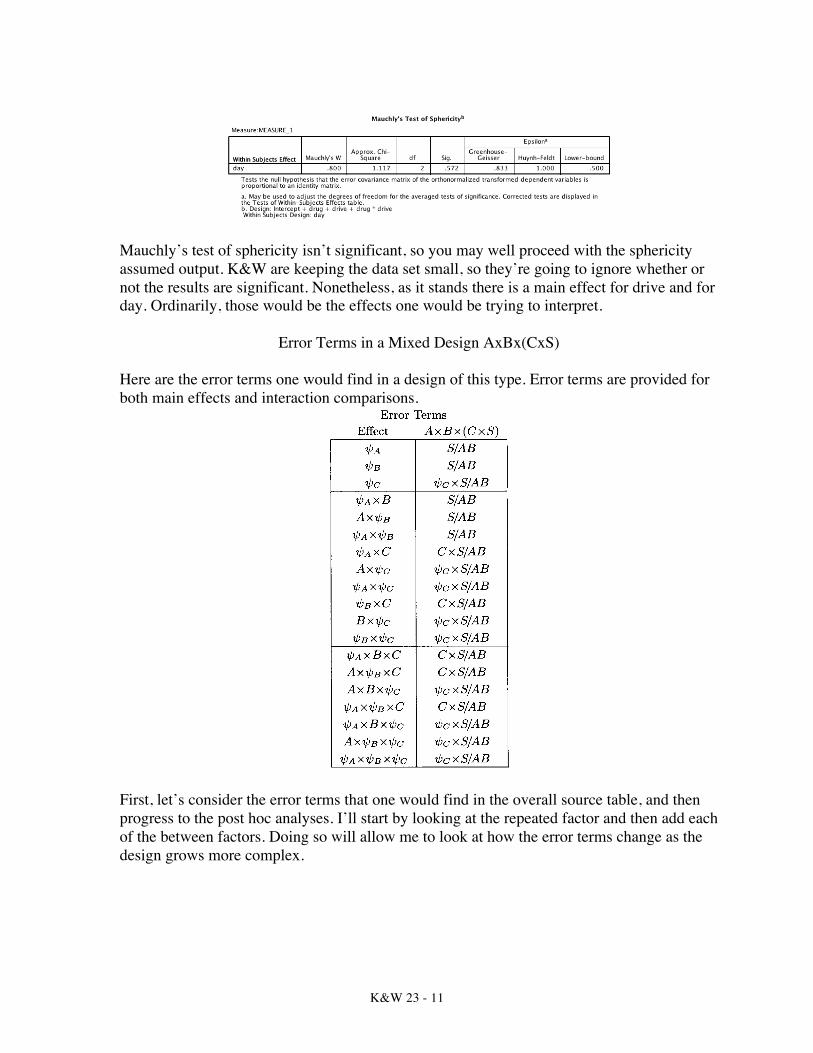
Mauchly’s test of sphericity isn’t significant, so you may well proceed with the sphericity assumed output. K&W are keeping the data set small, so they’re going to ignore whether or not the results are significant. Nonetheless, as it stands there is a main effect for drive and for day. Ordinarily, those would be the effects one would be trying to interpret.

Error Terms in a Mixed Design AxBx(CxS) Here are the error terms one would find in a design of this type. Error terms are provided for both main effects and interaction comparisons.

First, let’s consider the error terms that one would find in the overall source table, and then progress to the post hoc analyses. I’ll start by looking at the repeated factor and then add each of the between factors. Doing so will allow me to look at how the error terms change as the design grows more complex.

K&W 23 - 12

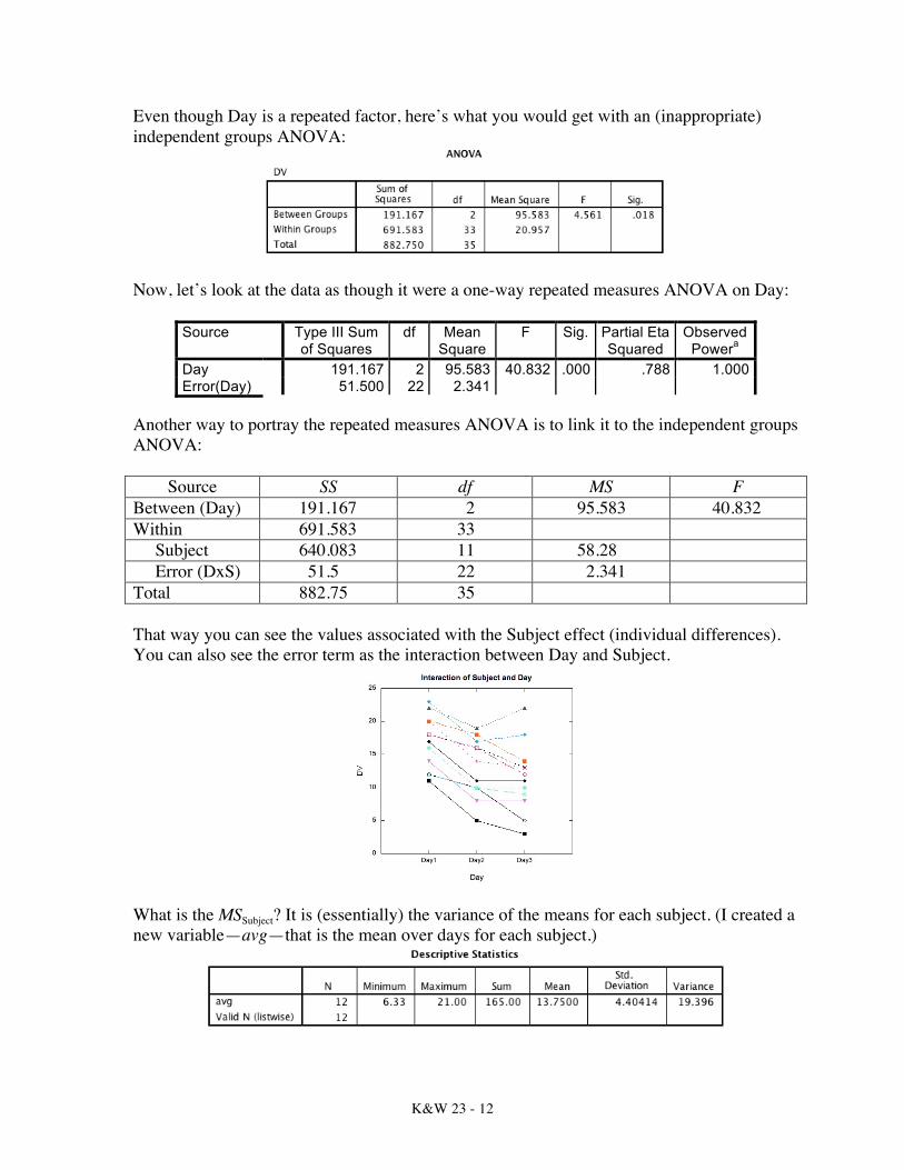
Even though Day is a repeated factor, here’s what you would get with an (inappropriate) independent groups ANOVA:

Now, let’s look at the data as though it were a one-way repeated measures ANOVA on Day:

Source Type III Sum of Squares

df Mean Square

F Sig. Partial Eta Squared

Observed Powera

Day 191.167 2 95.583 40.832 .000 .788 1.000 Error(Day) 51.500 22 2.341

Another way to portray the repeated measures ANOVA is to link it to the independent groups ANOVA:

Source SS df MS F Between (Day) 191.167 2 95.583 40.832 Within 691.583 33 Subject 640.083 11 58.28 Error (DxS) 51.5 22 2.341 Total 882.75 35 That way you can see the values associated with the Subject effect (individual differences). You can also see the error term as the interaction between Day and Subject.

What is the MSSubject? It is (essentially) the variance of the means for each subject. (I created a new variable—avg—that is the mean over days for each subject.)

K&W 23 - 13

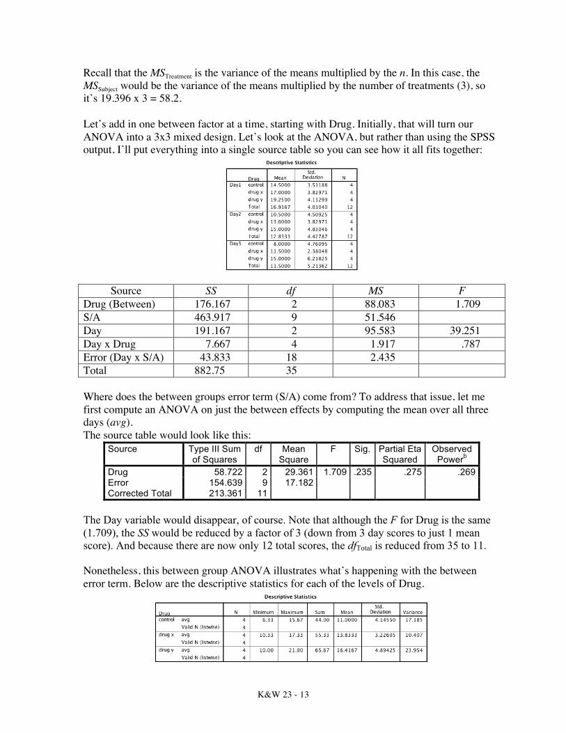
Recall that the MSTreatment is the variance of the means multiplied by the n. In this case, the MSSubject would be the variance of the means multiplied by the number of treatments (3), so it’s 19.396 x 3 = 58.2. Let’s add in one between factor at a time, starting with Drug. Initially, that will turn our ANOVA into a 3x3 mixed design. Let’s look at the ANOVA, but rather than using the SPSS output, I’ll put everything into a single source table so you can see how it all fits together:

Source SS df MS F Drug (Between) 176.167 2 88.083 1.709 S/A 463.917 9 51.546 Day 191.167 2 95.583 39.251 Day x Drug 7.667 4 1.917 .787 Error (Day x S/A) 43.833 18 2.435 Total 882.75 35 Where does the between groups error term (S/A) come from? To address that issue, let me first compute an ANOVA on just the between effects by computing the mean over all three days (avg). The source table would look like this:

Source Type III Sum of Squares

df Mean Square

F Sig. Partial Eta Squared

Observed Powerb

Drug 58.722 2 29.361 1.709 .235 .275 .269 Error 154.639 9 17.182 Corrected Total 213.361 11

The Day variable would disappear, of course. Note that although the F for Drug is the same (1.709), the SS would be reduced by a factor of 3 (down from 3 day scores to just 1 mean score). And because there are now only 12 total scores, the dfTotal is reduced from 35 to 11. Nonetheless, this between group ANOVA illustrates what’s happening with the between error term. Below are the descriptive statistics for each of the levels of Drug.

K&W 23 - 14

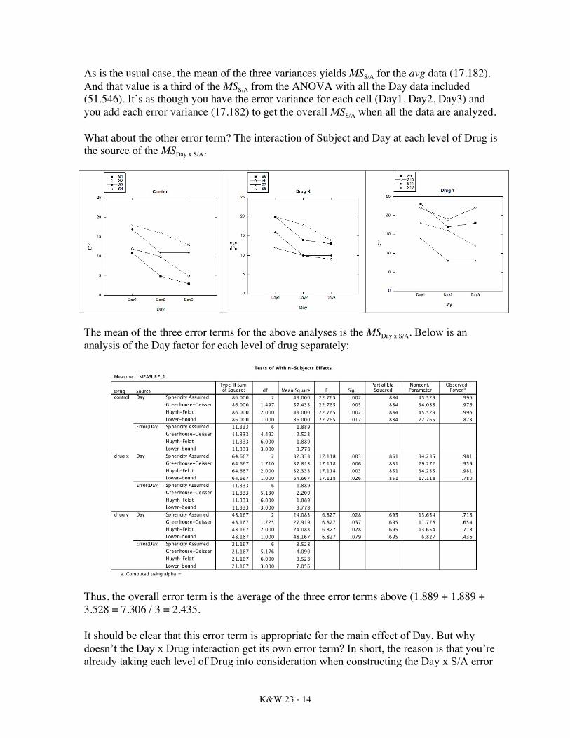
As is the usual case, the mean of the three variances yields MSS/A for the avg data (17.182). And that value is a third of the MSS/A from the ANOVA with all the Day data included (51.546). It’s as though you have the error variance for each cell (Day1, Day2, Day3) and you add each error variance (17.182) to get the overall MSS/A when all the data are analyzed. What about the other error term? The interaction of Subject and Day at each level of Drug is the source of the MSDay x S/A.

The mean of the three error terms for the above analyses is the MSDay x S/A. Below is an analysis of the Day factor for each level of drug separately:

Thus, the overall error term is the average of the three error terms above (1.889 + 1.889 + 3.528 = 7.306 / 3 = 2.435. It should be clear that this error term is appropriate for the main effect of Day. But why doesn’t the Day x Drug interaction get its own error term? In short, the reason is that you’re already taking each level of Drug into consideration when constructing the Day x S/A error

K&W 23 - 15

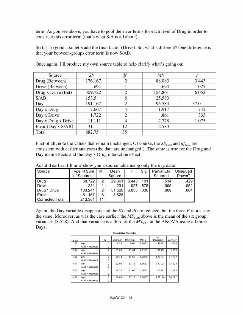
term. As you see above, you have to pool the error terms for each level of Drug in order to construct this error term (that’s what S/A is all about). So far, so good…so let’s add the final factor (Drive). So, what’s different? One difference is that your between-groups error term is now S/AB. Once again, I’ll produce my own source table to help clarify what’s going on:

Source SS df MS F Drug (Between) 176.167 2 88.083 3.443 Drive (Between) .694 1 .694 .027 Drug x Drive (Bet) 309.722 2 154.861 6.053 S/AB 153.5 6 25.583 Day 191.167 2 95.583 37.0 Day x Drug 7.667 4 1.917 .742 Day x Drive 1.722 2 .861 .333 Day x Drug x Drive 11.111 4 2.778 1.075 Error (Day x S/AB) 31 12 2.583 Total 882.75 35 First of all, note the values that remain unchanged. Of course, the SSTotal and dfTotal are consistent with earlier analyses (the data are unchanged!). The same is true for the Drug and Day main effects and the Day x Drug interaction effect. As I did earlier, I’ll now show you a source table using only the avg data: Source Type III Sum

of Squares df Mean

Square F Sig. Partial Eta

Squared Observed

Powerb Drug 58.722 2 29.361 3.443 .101 .534 .429 Drive .231 1 .231 .027 .875 .005 .052 Drug * Drive 103.241 2 51.620 6.053 .036 .669 .664 Error 51.167 6 8.528 Corrected Total 213.361 11

Again, the Day variable disappears and the SS and df are reduced, but the three F ratios stay the same. Moreover, as was the case earlier, the MSS/AB above is the mean of the six group variances (8.528). And that variance is a third of the MSS/AB in the ANOVA using all three Days.

K&W 23 - 16

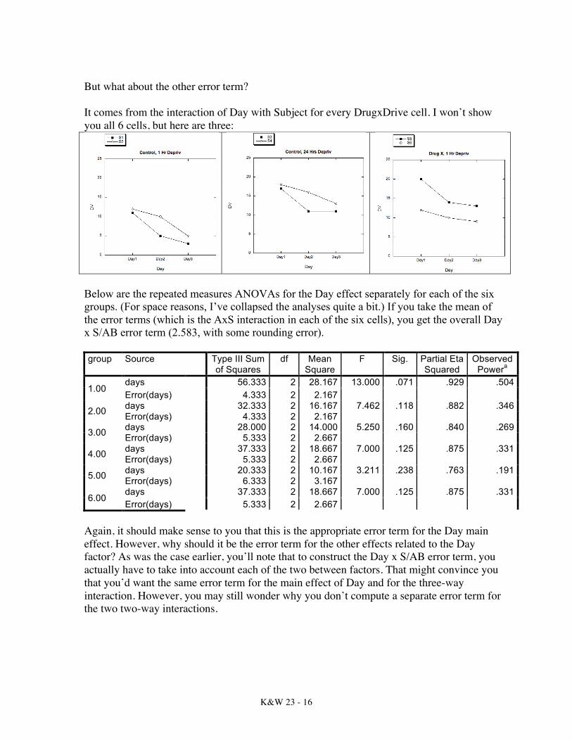
But what about the other error term? It comes from the interaction of Day with Subject for every DrugxDrive cell. I won’t show you all 6 cells, but here are three:

Below are the repeated measures ANOVAs for the Day effect separately for each of the six groups. (For space reasons, I’ve collapsed the analyses quite a bit.) If you take the mean of the error terms (which is the AxS interaction in each of the six cells), you get the overall Day x S/AB error term (2.583, with some rounding error). group Source Type III Sum

of Squares df Mean

Square F Sig. Partial Eta

Squared Observed

Powera

1.00 days 56.333 2 28.167 13.000 .071 .929 .504 Error(days) 4.333 2 2.167

2.00 days 32.333 2 16.167 7.462 .118 .882 .346 Error(days) 4.333 2 2.167

3.00 days 28.000 2 14.000 5.250 .160 .840 .269 Error(days) 5.333 2 2.667

4.00 days 37.333 2 18.667 7.000 .125 .875 .331 Error(days) 5.333 2 2.667

5.00 days 20.333 2 10.167 3.211 .238 .763 .191 Error(days) 6.333 2 3.167

6.00 days 37.333 2 18.667 7.000 .125 .875 .331 Error(days) 5.333 2 2.667

Again, it should make sense to you that this is the appropriate error term for the Day main effect. However, why should it be the error term for the other effects related to the Day factor? As was the case earlier, you’ll note that to construct the Day x S/AB error term, you actually have to take into account each of the two between factors. That might convince you that you’d want the same error term for the main effect of Day and for the three-way interaction. However, you may still wonder why you don’t compute a separate error term for the two two-way interactions.

K&W 23 - 17

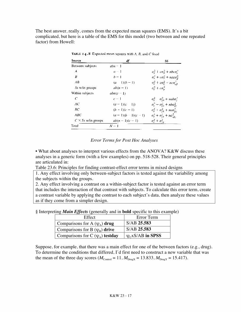
The best answer, really, comes from the expected mean squares (EMS). It’s a bit complicated, but here is a table of the EMS for this model (two between and one repeated factor) from Howell:

Error Terms for Post Hoc Analyses • What about analyses to interpret various effects from the ANOVA? K&W discuss these analyses in a generic form (with a few examples) on pp. 518-528. Their general principles are articulated in: Table 23.6: Principles for finding contrast-effect error terms in mixed designs 1. Any effect involving only between-subject factors is tested against the variability among the subjects within the groups. 2. Any effect involving a contrast on a within-subject factor is tested against an error term that includes the interaction of that contrast with subjects. To calculate this error term, create a contrast variable by applying the contrast to each subject’s data, then analyze these values as if they come from a simpler design. § Interpreting Main Effects (generally and in bold specific to this example)

Effect Error Term Comparisons for A (ψA) drug S/AB 25.583 Comparisons for B (ψB) drive S/AB 25.583 Comparisons for C (ψA) testday ψCxS/AB in SPSS

Suppose, for example, that there was a main effect for one of the between factors (e.g., drug). To determine the conditions that differed, I’d first need to construct a new variable that was the mean of the three day scores (MControl = 11, MDrugX = 13.833, MDrugY = 15.417).

K&W 23 - 18

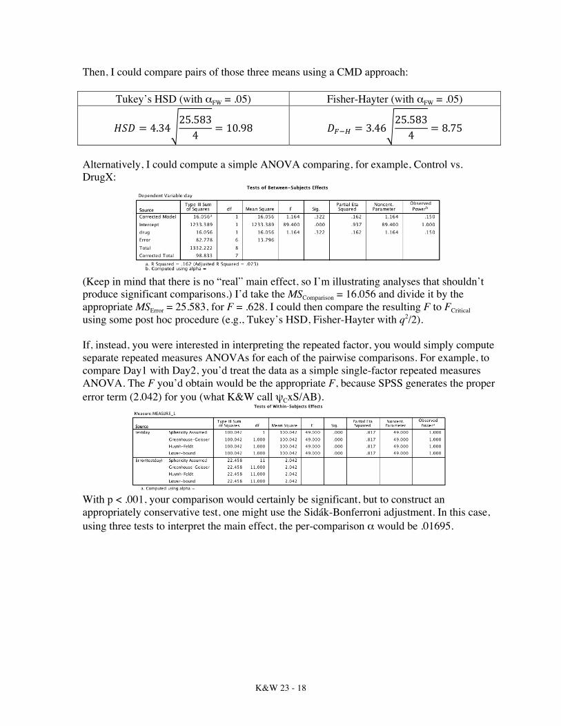
Then, I could compare pairs of those three means using a CMD approach:

Tukey’s HSD (with αFW = .05) Fisher-Hayter (with αFW = .05)

𝐻𝑆𝐷 = 4.3425.5834 = 10.98 𝐷!!! = 3.46

25.5834 = 8.75

Alternatively, I could compute a simple ANOVA comparing, for example, Control vs. DrugX:

(Keep in mind that there is no “real” main effect, so I’m illustrating analyses that shouldn’t produce significant comparisons.) I’d take the MSComparison = 16.056 and divide it by the appropriate MSError = 25.583, for F = .628. I could then compare the resulting F to FCritical using some post hoc procedure (e.g., Tukey’s HSD, Fisher-Hayter with q2/2). If, instead, you were interested in interpreting the repeated factor, you would simply compute separate repeated measures ANOVAs for each of the pairwise comparisons. For example, to compare Day1 with Day2, you’d treat the data as a simple single-factor repeated measures ANOVA. The F you’d obtain would be the appropriate F, because SPSS generates the proper error term (2.042) for you (what K&W call ψCxS/AB).

With p < .001, your comparison would certainly be significant, but to construct an appropriately conservative test, one might use the Sidák-Bonferroni adjustment. In this case, using three tests to interpret the main effect, the per-comparison α would be .01695.

K&W 23 - 19

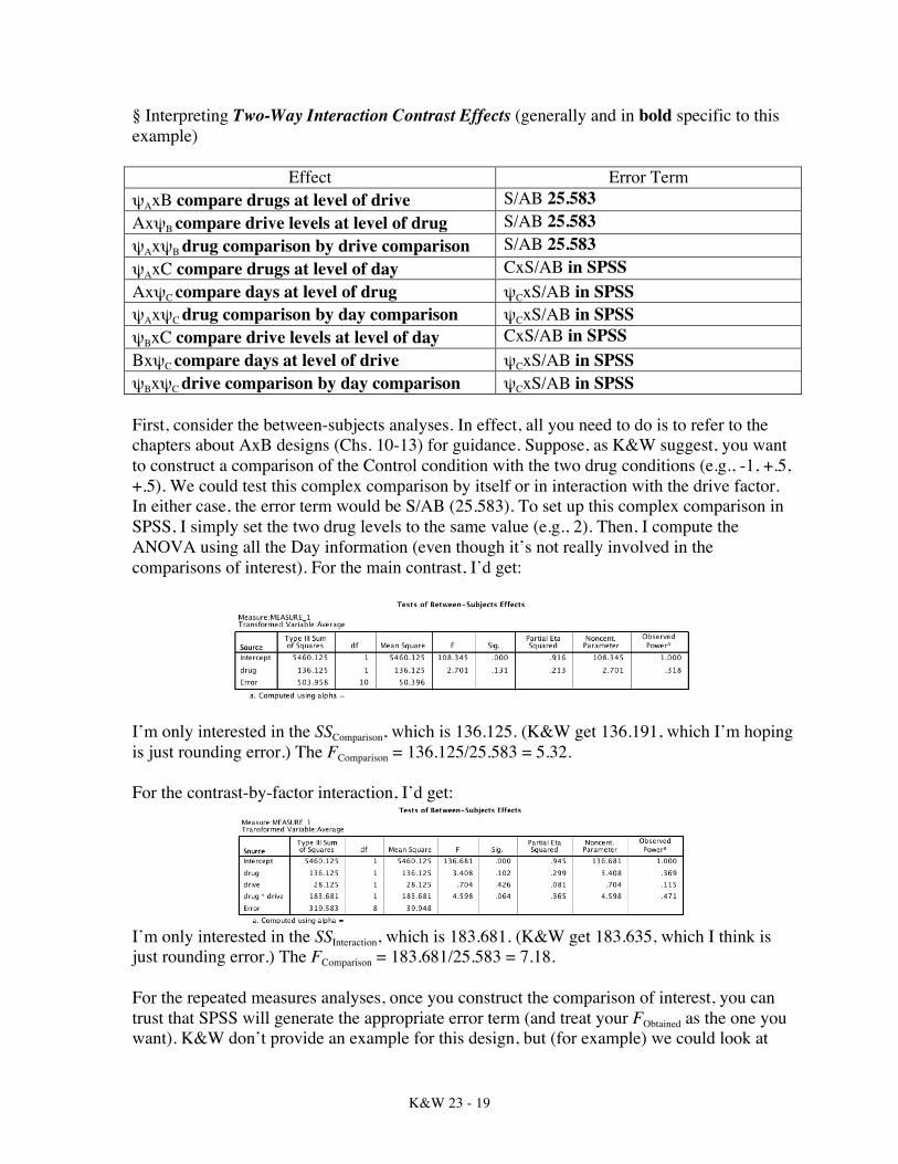
§ Interpreting Two-Way Interaction Contrast Effects (generally and in bold specific to this example)

Effect Error Term ψAxB compare drugs at level of drive S/AB 25.583 AxψB compare drive levels at level of drug S/AB 25.583 ψAxψB drug comparison by drive comparison S/AB 25.583 ψAxC compare drugs at level of day CxS/AB in SPSS AxψC compare days at level of drug ψCxS/AB in SPSS ψAxψC drug comparison by day comparison ψCxS/AB in SPSS ψBxC compare drive levels at level of day CxS/AB in SPSS BxψC compare days at level of drive ψCxS/AB in SPSS ψBxψC drive comparison by day comparison ψCxS/AB in SPSS First, consider the between-subjects analyses. In effect, all you need to do is to refer to the chapters about AxB designs (Chs. 10-13) for guidance. Suppose, as K&W suggest, you want to construct a comparison of the Control condition with the two drug conditions (e.g., -1, +.5, +.5). We could test this complex comparison by itself or in interaction with the drive factor. In either case, the error term would be S/AB (25.583). To set up this complex comparison in SPSS, I simply set the two drug levels to the same value (e.g., 2). Then, I compute the ANOVA using all the Day information (even though it’s not really involved in the comparisons of interest). For the main contrast, I’d get:

I’m only interested in the SSComparison, which is 136.125. (K&W get 136.191, which I’m hoping is just rounding error.) The FComparison = 136.125/25.583 = 5.32. For the contrast-by-factor interaction, I’d get:

I’m only interested in the SSInteraction, which is 183.681. (K&W get 183.635, which I think is just rounding error.) The FComparison = 183.681/25.583 = 7.18. For the repeated measures analyses, once you construct the comparison of interest, you can trust that SPSS will generate the appropriate error term (and treat your FObtained as the one you want). K&W don’t provide an example for this design, but (for example) we could look at

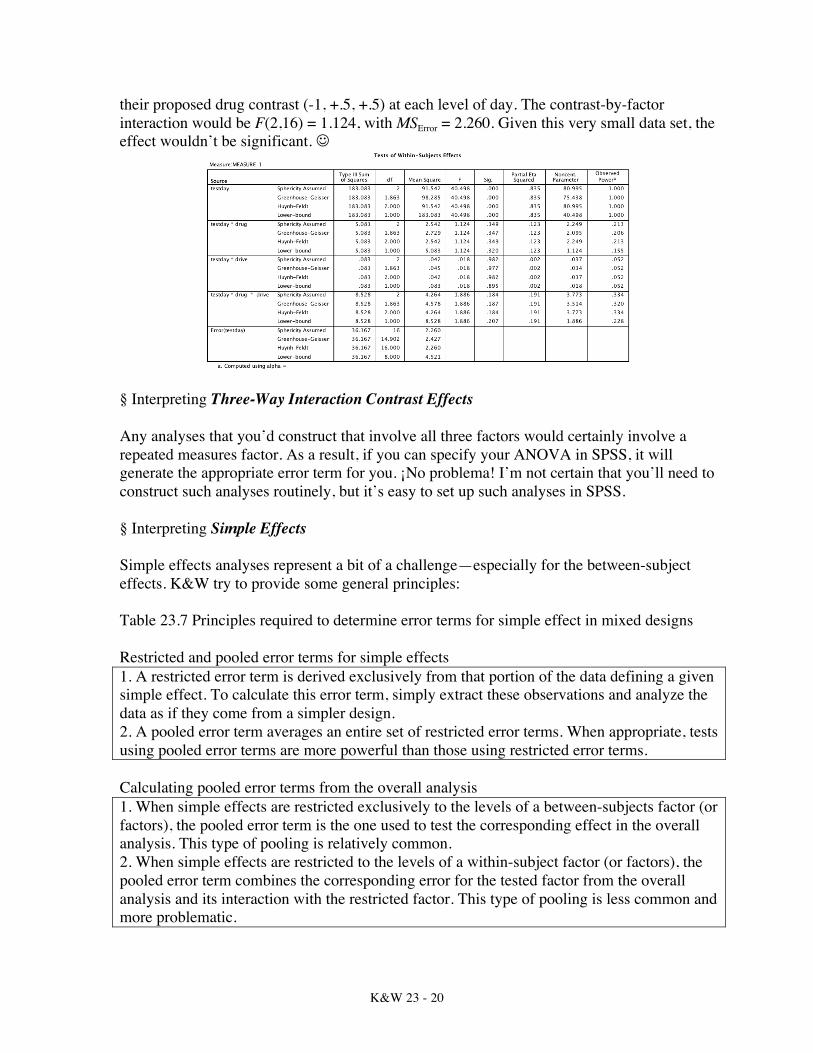
K&W 23 - 20

their proposed drug contrast (-1, +.5, +.5) at each level of day. The contrast-by-factor interaction would be F(2,16) = 1.124, with MSError = 2.260. Given this very small data set, the effect wouldn’t be significant. J

§ Interpreting Three-Way Interaction Contrast Effects Any analyses that you’d construct that involve all three factors would certainly involve a repeated measures factor. As a result, if you can specify your ANOVA in SPSS, it will generate the appropriate error term for you. ¡No problema! I’m not certain that you’ll need to construct such analyses routinely, but it’s easy to set up such analyses in SPSS. § Interpreting Simple Effects Simple effects analyses represent a bit of a challenge—especially for the between-subject effects. K&W try to provide some general principles: Table 23.7 Principles required to determine error terms for simple effect in mixed designs Restricted and pooled error terms for simple effects 1. A restricted error term is derived exclusively from that portion of the data defining a given simple effect. To calculate this error term, simply extract these observations and analyze the data as if they come from a simpler design. 2. A pooled error term averages an entire set of restricted error terms. When appropriate, tests using pooled error terms are more powerful than those using restricted error terms. Calculating pooled error terms from the overall analysis 1. When simple effects are restricted exclusively to the levels of a between-subjects factor (or factors), the pooled error term is the one used to test the corresponding effect in the overall analysis. This type of pooling is relatively common. 2. When simple effects are restricted to the levels of a within-subject factor (or factors), the pooled error term combines the corresponding error for the tested factor from the overall analysis and its interaction with the restricted factor. This type of pooling is less common and more problematic.

K&W 23 - 21

As a result, you have some suggested error terms in Table 23.8. I won’t bother repeating all of them here, but instead provide only a sampling of the ones that I think you’d find most useful for this AxBx(CxS) design.

Effect Restricted Pooled Compare levels of A @ one level of B S/AB Compare levels of B @ one level of A S/AB Compare levels of A @ one level of C S/AB @ that level of C S/AB + CxS/AB Compare levels of C @ one level of A ψCxS/B at a CxS/AB Compare levels of C @ one level of B ψCxS/A at b CxS/AB • Suppose, for example, as K&W illustrate, you’re interested in the simple effect of a between-subjects factor such as drug (or drive, except that it has only two levels) only on Day 3. You can see the results of that analysis in Table 23.10 (p. 526), or in the SPSS analysis below:

The F for drug (for example) is obtained using the restricted error term, which is what SPSS produces. However, if you were interested in the pooled error term, you would return to the original overall ANOVA and add together the S/AB and CxS/AB effects to form MSError:

𝑀𝑆!""#" =153.5+ 316+ 12 = 10.25

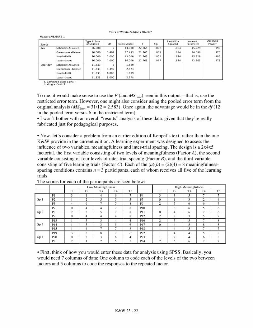
For this simple effect, F = 49/10.25 = 4.78. As K&W note, the real advantage is in the increased df that are attached to this pooled error term. You wouldn’t find a significant simple effect for drug on Day3 in this particular case, but the strategy is a sound one nonetheless. You would be able to test your F using FCrit(2,18) = 3.55, which would be an advantage. In this particular case, however, you’d be better off with the restricted error term. • Suppose that instead you were interested in the simple effects of a within-subjects factor. In this example, we could look at the effects of Day at each level of drug. Here is the output for the Control condition (and, using Split File, you’d have output for the other two levels as well):

K&W 23 - 22

To me, it would make sense to use the F (and MSError) seen in this output—that is, use the restricted error term. However, one might also consider using the pooled error term from the original analysis (MSError = 31/12 = 2.583). Once again, the advantage would be in the df (12 in the pooled term versus 6 in the restricted term). • I won’t bother with an overall “results” analysis of these data, given that they’re really fabricated just for pedagogical purposes. • Now, let’s consider a problem from an earlier edition of Keppel’s text, rather than the one K&W provide in the current edition. A learning experiment was designed to assess the influence of two variables, meaningfulness and inter-trial spacing. The design is a 2x4x5 factorial, the first variable consisting of two levels of meaningfulness (Factor A), the second variable consisting of four levels of inter-trial spacing (Factor B), and the third variable consisting of five learning trials (Factor C). Each of the (a)(b) = (2)(4) = 8 meaningfulness-spacing conditions contains n = 3 participants, each of whom receives all five of the learning trials. The scores for each of the participants are seen below: Low Meaningfulness High Meaningfulness T1 T2 T3 T4 T5 T1 T2 T3 T4 T5 Sp 1

P1 3 1 4 6 7 P4 3 3 5 7 7 P2 1 2 5 5 5 P5 0 1 3 2 4 P3 4 6 7 7 8 P6 2 5 6 6 7

Sp 2

P7 0 4 4 7 8 P10 1 3 6 5 6 P8 2 3 5 7 8 P11 0 4 6 7 6 P9 0 4 4 4 8 P12 2 2 3 5 7

Sp 3

P13 1 3 3 4 4 P16 2 3 5 7 8 P14 1 3 3 5 6 P17 0 4 5 8 8 P15 1 4 7 7 8 P18 1 4 5 7 7

Sp 4

P19 3 5 8 7 6 P22 1 4 4 5 8 P20 0 2 3 6 4 P23 1 2 4 6 8 P21 2 1 2 5 5 P24 2 5 6 7 7

• First, think of how you would enter these data for analysis using SPSS. Basically, you would need 7 columns of data: One column to code each of the levels of the two between factors and 5 columns to code the responses to the repeated factor.

K&W 23 - 23

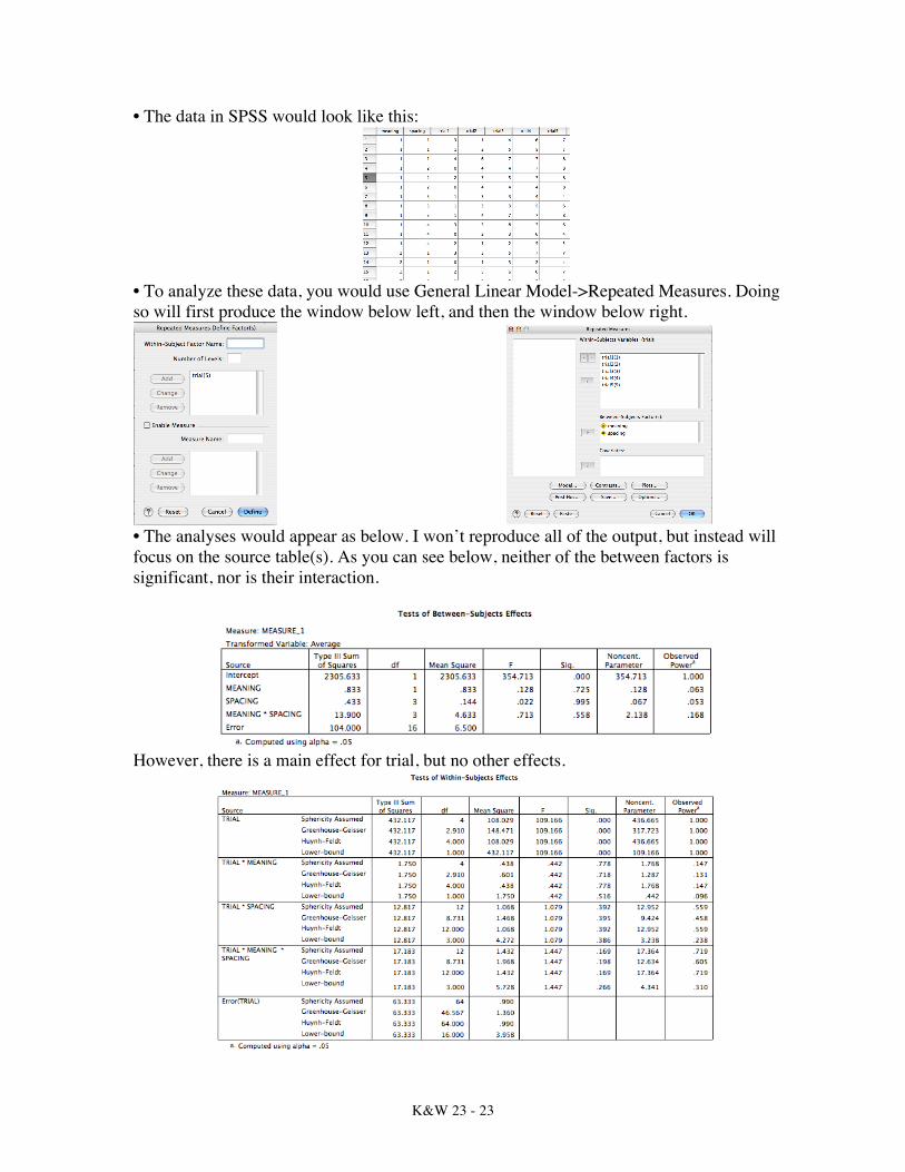
• The data in SPSS would look like this:

• To analyze these data, you would use General Linear Model->Repeated Measures. Doing so will first produce the window below left, and then the window below right.

• The analyses would appear as below. I won’t reproduce all of the output, but instead will focus on the source table(s). As you can see below, neither of the between factors is significant, nor is their interaction.

However, there is a main effect for trial, but no other effects.

K&W 23 - 24

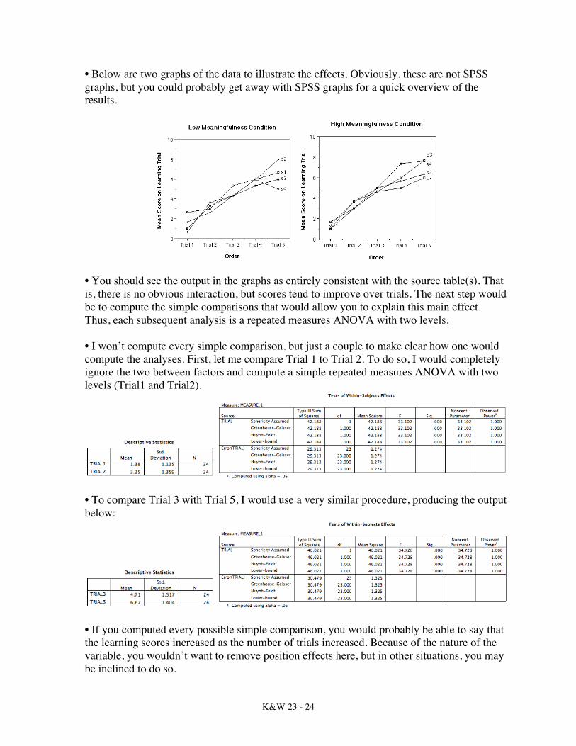
• Below are two graphs of the data to illustrate the effects. Obviously, these are not SPSS graphs, but you could probably get away with SPSS graphs for a quick overview of the results.

• You should see the output in the graphs as entirely consistent with the source table(s). That is, there is no obvious interaction, but scores tend to improve over trials. The next step would be to compute the simple comparisons that would allow you to explain this main effect. Thus, each subsequent analysis is a repeated measures ANOVA with two levels. • I won’t compute every simple comparison, but just a couple to make clear how one would compute the analyses. First, let me compare Trial 1 to Trial 2. To do so, I would completely ignore the two between factors and compute a simple repeated measures ANOVA with two levels (Trial1 and Trial2).

• To compare Trial 3 with Trial 5, I would use a very similar procedure, producing the output below:

• If you computed every possible simple comparison, you would probably be able to say that the learning scores increased as the number of trials increased. Because of the nature of the variable, you wouldn’t want to remove position effects here, but in other situations, you may be inclined to do so.

K&W 23 - 25

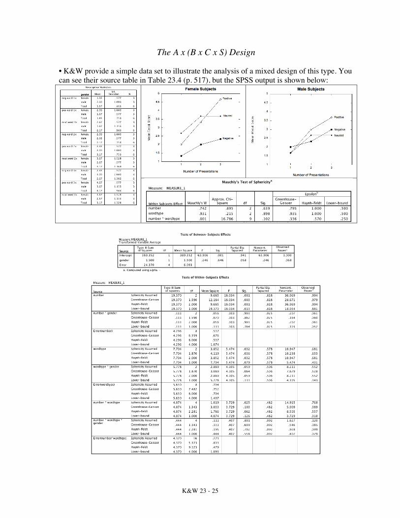
The A x (B x C x S) Design • K&W provide a simple data set to illustrate the analysis of a mixed design of this type. You can see their source table in Table 23.4 (p. 517), but the SPSS output is shown below:

K&W 23 - 26

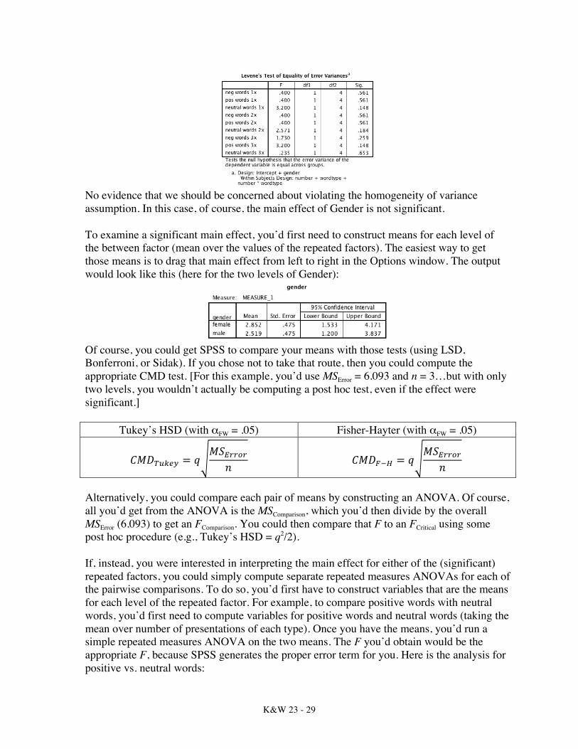
As they describe the memory (recall) study, male and female college students see a list of words to study, with a third positive, a third neutral, and a third negative. A third of the words of each type are presented once, a third presented two times, and a third presented three times. Thus, it’s a 2 (gender) x 3 (word type) x 3 (number of presentations) design. • K&W are really focused more on providing a simple data set from which they can make points about analysis, so we won’t make too much of these analyses. Nonetheless, it’s clear that there would be a main effect for word type, F(2,8) = 5.47, MSE = .704, p = .032, η2 = .578. There would also be a main effect for number of presentations, F(2,8) = 18.034, MSE = .537, p = .001, η2 = .818. There would also be an interaction between number of presentations and word type, F(4,16) = 3.729, MSE = .273, p = .025, η2 = .482. For some reason, K&W don’t think that this interaction is significant. However, they do think that the gender by word type interaction is significant, but SPSS says that it’s not quite significant (p = .059). Oh, well. J

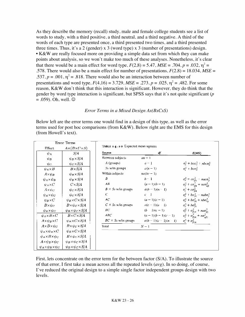
Error Terms in a Mixed Design Ax(BxCxS) Below left are the error terms one would find in a design of this type, as well as the error terms used for post hoc comparisons (from K&W). Below right are the EMS for this design (from Howell’s text).

First, lets concentrate on the error term for the between factor (S/A). To illustrate the source of that error, I first take a mean across all the repeated levels (avg). In so doing, of course, I’ve reduced the original design to a simple single factor independent groups design with two levels.

K&W 23 - 27

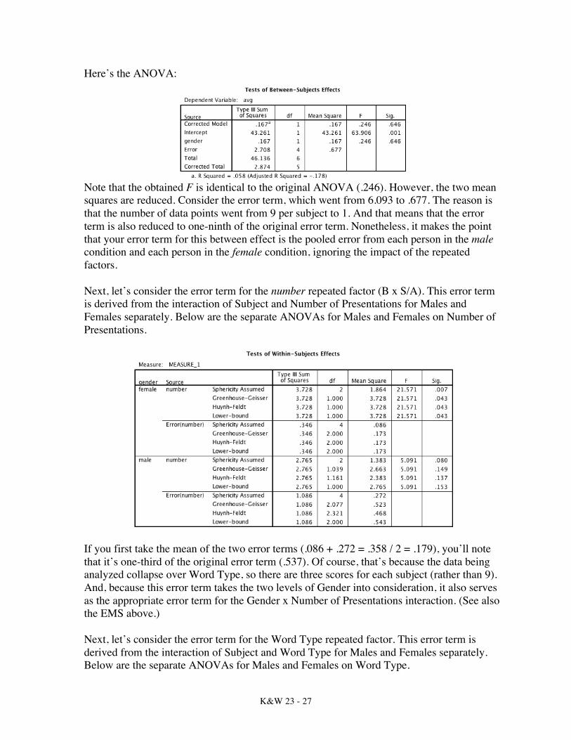
Here’s the ANOVA:

Note that the obtained F is identical to the original ANOVA (.246). However, the two mean squares are reduced. Consider the error term, which went from 6.093 to .677. The reason is that the number of data points went from 9 per subject to 1. And that means that the error term is also reduced to one-ninth of the original error term. Nonetheless, it makes the point that your error term for this between effect is the pooled error from each person in the male condition and each person in the female condition, ignoring the impact of the repeated factors. Next, let’s consider the error term for the number repeated factor (B x S/A). This error term is derived from the interaction of Subject and Number of Presentations for Males and Females separately. Below are the separate ANOVAs for Males and Females on Number of Presentations.

If you first take the mean of the two error terms (.086 + .272 = .358 / 2 = .179), you’ll note that it’s one-third of the original error term (.537). Of course, that’s because the data being analyzed collapse over Word Type, so there are three scores for each subject (rather than 9). And, because this error term takes the two levels of Gender into consideration, it also serves as the appropriate error term for the Gender x Number of Presentations interaction. (See also the EMS above.) Next, let’s consider the error term for the Word Type repeated factor. This error term is derived from the interaction of Subject and Word Type for Males and Females separately. Below are the separate ANOVAs for Males and Females on Word Type.

K&W 23 - 28

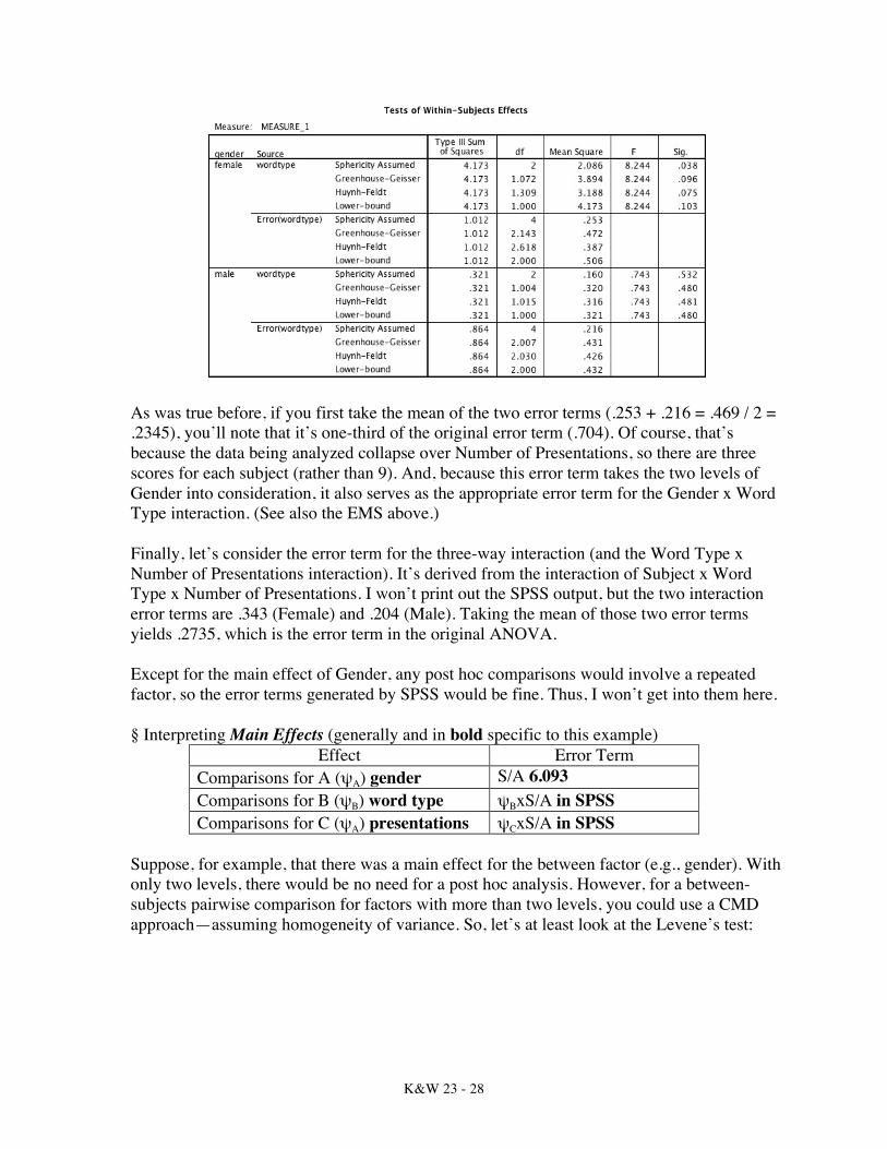
As was true before, if you first take the mean of the two error terms (.253 + .216 = .469 / 2 = .2345), you’ll note that it’s one-third of the original error term (.704). Of course, that’s because the data being analyzed collapse over Number of Presentations, so there are three scores for each subject (rather than 9). And, because this error term takes the two levels of Gender into consideration, it also serves as the appropriate error term for the Gender x Word Type interaction. (See also the EMS above.) Finally, let’s consider the error term for the three-way interaction (and the Word Type x Number of Presentations interaction). It’s derived from the interaction of Subject x Word Type x Number of Presentations. I won’t print out the SPSS output, but the two interaction error terms are .343 (Female) and .204 (Male). Taking the mean of those two error terms yields .2735, which is the error term in the original ANOVA. Except for the main effect of Gender, any post hoc comparisons would involve a repeated factor, so the error terms generated by SPSS would be fine. Thus, I won’t get into them here. § Interpreting Main Effects (generally and in bold specific to this example)

Effect Error Term Comparisons for A (ψA) gender S/A 6.093 Comparisons for B (ψB) word type ψBxS/A in SPSS Comparisons for C (ψA) presentations ψCxS/A in SPSS

Suppose, for example, that there was a main effect for the between factor (e.g., gender). With only two levels, there would be no need for a post hoc analysis. However, for a between-subjects pairwise comparison for factors with more than two levels, you could use a CMD approach—assuming homogeneity of variance. So, let’s at least look at the Levene’s test:

K&W 23 - 29

No evidence that we should be concerned about violating the homogeneity of variance assumption. In this case, of course, the main effect of Gender is not significant. To examine a significant main effect, you’d first need to construct means for each level of the between factor (mean over the values of the repeated factors). The easiest way to get those means is to drag that main effect from left to right in the Options window. The output would look like this (here for the two levels of Gender):

Of course, you could get SPSS to compare your means with those tests (using LSD, Bonferroni, or Sidak). If you chose not to take that route, then you could compute the appropriate CMD test. [For this example, you’d use MSError = 6.093 and n = 3…but with only two levels, you wouldn’t actually be computing a post hoc test, even if the effect were significant.]

Tukey’s HSD (with αFW = .05) Fisher-Hayter (with αFW = .05)

𝐶𝑀𝐷!"#$% = 𝑞𝑀𝑆!""#"

𝑛 𝐶𝑀𝐷!!! = 𝑞𝑀𝑆!""#"

𝑛

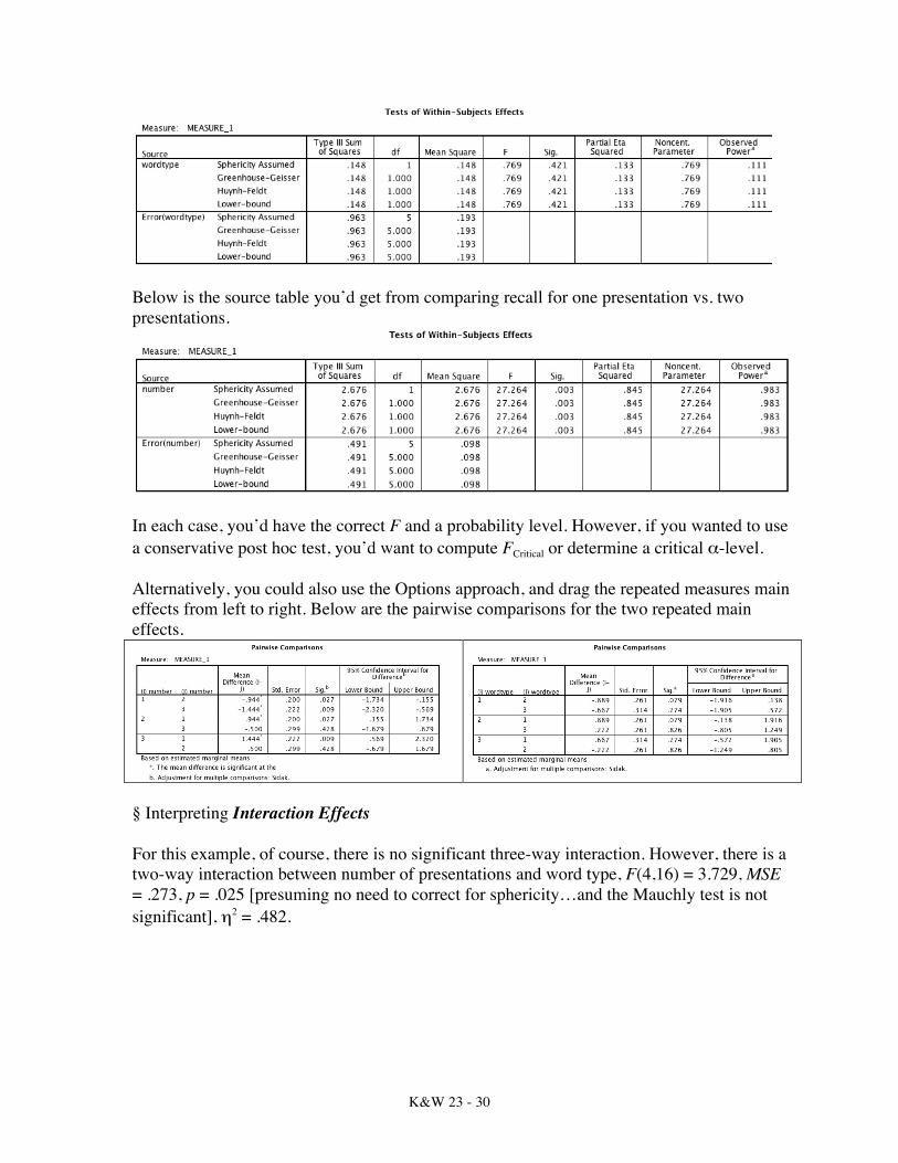
Alternatively, you could compare each pair of means by constructing an ANOVA. Of course, all you’d get from the ANOVA is the MSComparison, which you’d then divide by the overall MSError (6.093) to get an FComparison. You could then compare that F to an FCritical using some post hoc procedure (e.g., Tukey’s HSD = q2/2). If, instead, you were interested in interpreting the main effect for either of the (significant) repeated factors, you could simply compute separate repeated measures ANOVAs for each of the pairwise comparisons. To do so, you’d first have to construct variables that are the means for each level of the repeated factor. For example, to compare positive words with neutral words, you’d first need to compute variables for positive words and neutral words (taking the mean over number of presentations of each type). Once you have the means, you’d run a simple repeated measures ANOVA on the two means. The F you’d obtain would be the appropriate F, because SPSS generates the proper error term for you. Here is the analysis for positive vs. neutral words:

K&W 23 - 30

Below is the source table you’d get from comparing recall for one presentation vs. two presentations.

In each case, you’d have the correct F and a probability level. However, if you wanted to use a conservative post hoc test, you’d want to compute FCritical or determine a critical α-level. Alternatively, you could also use the Options approach, and drag the repeated measures main effects from left to right. Below are the pairwise comparisons for the two repeated main effects.

§ Interpreting Interaction Effects For this example, of course, there is no significant three-way interaction. However, there is a two-way interaction between number of presentations and word type, F(4,16) = 3.729, MSE = .273, p = .025 [presuming no need to correct for sphericity…and the Mauchly test is not significant], η2 = .482.

K&W 23 - 31

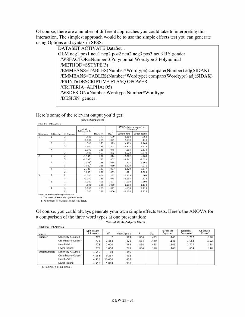
Of course, there are a number of different approaches you could take to interpreting this interaction. The simplest approach would be to use the simple effects test you can generate using Options and syntax in SPSS:

DATASET ACTIVATE DataSet1. GLM neg1 pos1 neu1 neg2 pos2 neu2 neg3 pos3 neu3 BY gender /WSFACTOR=Number 3 Polynomial Wordtype 3 Polynomial /METHOD=SSTYPE(3) /EMMEANS=TABLES(Number*Wordtype) compare(Number) adj(SIDAK) /EMMEANS=TABLES(Number*Wordtype) compare(Wordtype) adj(SIDAK) /PRINT=DESCRIPTIVE ETASQ OPOWER /CRITERIA=ALPHA(.05) /WSDESIGN=Number Wordtype Number*Wordtype /DESIGN=gender.

Here’s some of the relevant output you’d get:

Of course, you could always generate your own simple effects tests. Here’s the ANOVA for a comparison of the three word types at one presentation:

K&W 23 - 32

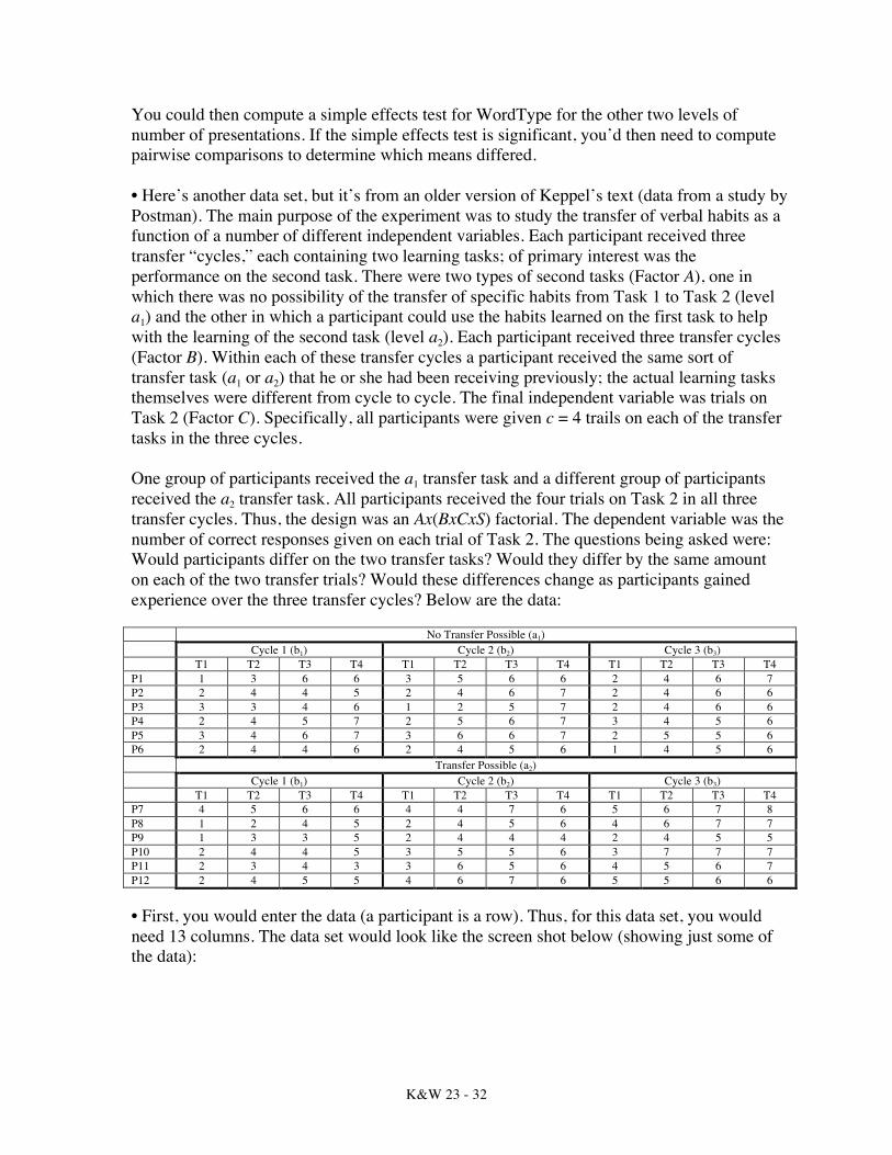
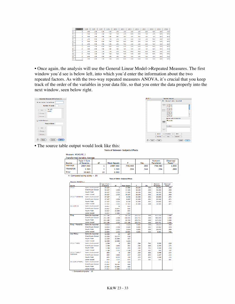
You could then compute a simple effects test for WordType for the other two levels of number of presentations. If the simple effects test is significant, you’d then need to compute pairwise comparisons to determine which means differed. • Here’s another data set, but it’s from an older version of Keppel’s text (data from a study by Postman). The main purpose of the experiment was to study the transfer of verbal habits as a function of a number of different independent variables. Each participant received three transfer “cycles,” each containing two learning tasks; of primary interest was the performance on the second task. There were two types of second tasks (Factor A), one in which there was no possibility of the transfer of specific habits from Task 1 to Task 2 (level a1) and the other in which a participant could use the habits learned on the first task to help with the learning of the second task (level a2). Each participant received three transfer cycles (Factor B). Within each of these transfer cycles a participant received the same sort of transfer task (a1 or a2) that he or she had been receiving previously; the actual learning tasks themselves were different from cycle to cycle. The final independent variable was trials on Task 2 (Factor C). Specifically, all participants were given c = 4 trails on each of the transfer tasks in the three cycles. One group of participants received the a1 transfer task and a different group of participants received the a2 transfer task. All participants received the four trials on Task 2 in all three transfer cycles. Thus, the design was an Ax(BxCxS) factorial. The dependent variable was the number of correct responses given on each trial of Task 2. The questions being asked were: Would participants differ on the two transfer tasks? Would they differ by the same amount on each of the two transfer trials? Would these differences change as participants gained experience over the three transfer cycles? Below are the data: No Transfer Possible (a1) Cycle 1 (b1) Cycle 2 (b2) Cycle 3 (b3) T1 T2 T3 T4 T1 T2 T3 T4 T1 T2 T3 T4 P1 1 3 6 6 3 5 6 6 2 4 6 7 P2 2 4 4 5 2 4 6 7 2 4 6 6 P3 3 3 4 6 1 2 5 7 2 4 6 6 P4 2 4 5 7 2 5 6 7 3 4 5 6 P5 3 4 6 7 3 6 6 7 2 5 5 6 P6 2 4 4 6 2 4 5 6 1 4 5 6 Transfer Possible (a2) Cycle 1 (b1) Cycle 2 (b2) Cycle 3 (b3) T1 T2 T3 T4 T1 T2 T3 T4 T1 T2 T3 T4 P7 4 5 6 6 4 4 7 6 5 6 7 8 P8 1 2 4 5 2 4 5 6 4 6 7 7 P9 1 3 3 5 2 4 4 4 2 4 5 5 P10 2 4 4 5 3 5 5 6 3 7 7 7 P11 2 3 4 3 3 6 5 6 4 5 6 7 P12 2 4 5 5 4 6 7 6 5 5 6 6 • First, you would enter the data (a participant is a row). Thus, for this data set, you would need 13 columns. The data set would look like the screen shot below (showing just some of the data):

K&W 23 - 33

• Once again, the analysis will use the General Linear Model->Repeated Measures. The first window you’d see is below left, into which you’d enter the information about the two repeated factors. As with the two-way repeated measures ANOVA, it’s crucial that you keep track of the order of the variables in your data file, so that you enter the data properly into the next window, seen below right.

• The source table output would look like this:

K&W 23 - 34

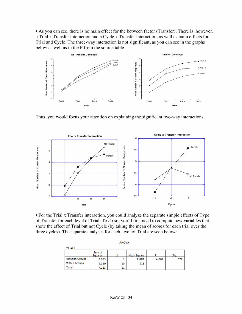
• As you can see, there is no main effect for the between factor (Transfer). There is, however, a Trial x Transfer interaction and a Cycle x Transfer interaction, as well as main effects for Trial and Cycle. The three-way interaction is not significant, as you can see in the graphs below as well as in the F from the source table.

Thus, you would focus your attention on explaining the significant two-way interactions.

• For the Trial x Transfer interaction, you could analyze the separate simple effects of Type of Transfer for each level of Trial. To do so, you’d first need to compute new variables that show the effect of Trial but not Cycle (by taking the mean of scores for each trial over the three cycles). The separate analyses for each level of Trial are seen below:

Trial 1 Trial 2 Trial 3 Trial 41

2

3

4

5

6

7

No Transfer Condition

Order

Mea

n Nu

mbe

r of C

orre

ct R

espo

nses

Cycle 1

Cycle 2Cycle 3

Trial 1 Trial 2 Trial 3 Trial 41

2

3

4

5

6

7

Transfer Condition

Order

Mea

n Nu

mbe

r of C

orre

ct R

espo

nses

Cycle 1

Cycle 2

Cycle 3

2

3

4

5

6

7

t1 t2 t3 t4

Trial x Transfer Interaction

Mea

n N

umbe

r of C

orre

ct R

espo

nses

Trial

No Transfer

Transfer

3.5

4

4.5

5

5.5

6

c1 c2 c3

Cycle x Transfer Interaction

Mea

n N

umbe

r of C

orre

ct R

espo

nses

Cycle

No Transfer

Transfer

K&W 23 - 35

Because these are between comparisons, with homogeneity of variance you would use a single MSError (not the MSError seen in each of the above ANOVAs). To get that MSError, I need to first compute the two-way ANOVA on the averaged Trial data. The source table would be:

To compute MSError, I would pool the two error terms in the above analysis:

€

MSError =4.069 +13.208

30 +10= .432

Trial 1 F = 2.083 / .432 = 4.82 Trial 2 F = .926 / .432 = 2.14 Trial 3 F = .009 / .432 = .02 Trial 4 F = 1.12 / .432 = 2.59

K&W 23 - 36

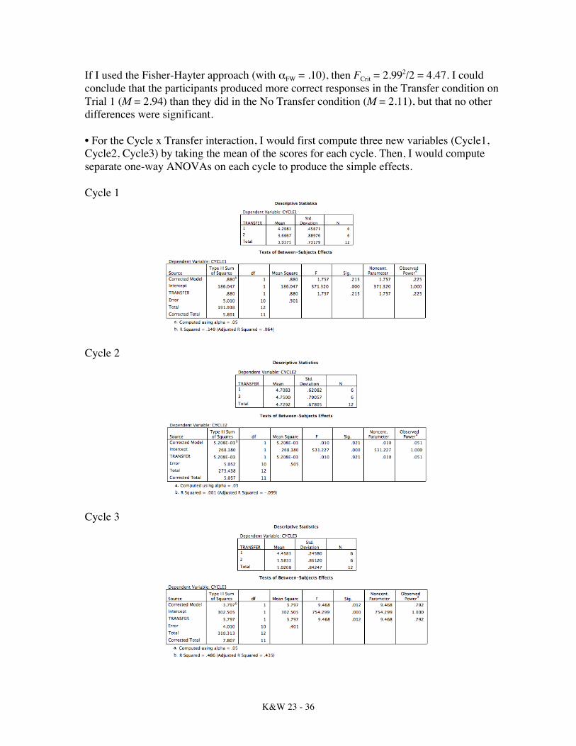
If I used the Fisher-Hayter approach (with αFW = .10), then FCrit = 2.992/2 = 4.47. I could conclude that the participants produced more correct responses in the Transfer condition on Trial 1 (M = 2.94) than they did in the No Transfer condition (M = 2.11), but that no other differences were significant. • For the Cycle x Transfer interaction, I would first compute three new variables (Cycle1, Cycle2, Cycle3) by taking the mean of the scores for each cycle. Then, I would compute separate one-way ANOVAs on each cycle to produce the simple effects. Cycle 1

Cycle 2

Cycle 3

K&W 23 - 37

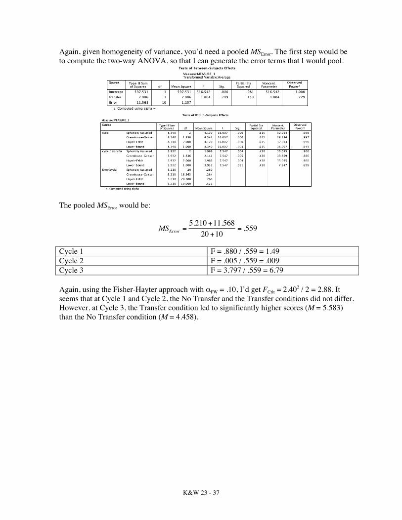
Again, given homogeneity of variance, you’d need a pooled MSError. The first step would be to compute the two-way ANOVA, so that I can generate the error terms that I would pool.

The pooled MSError would be:

€

MSError =5.210 +11.568

20 +10= .559

Cycle 1 F = .880 / .559 = 1.49 Cycle 2 F = .005 / .559 = .009 Cycle 3 F = 3.797 / .559 = 6.79 Again, using the Fisher-Hayter approach with αFW = .10, I’d get FCrit = 2.402 / 2 = 2.88. It seems that at Cycle 1 and Cycle 2, the No Transfer and the Transfer conditions did not differ. However, at Cycle 3, the Transfer condition led to significantly higher scores (M = 5.583) than the No Transfer condition (M = 4.458).