Kentucky’s Urban/Rural Landscape - University of …cedik.ca.uky.edu/files/kyruralurbanwealthdifferences.pdfKentucky’s Urban/Rural Landscape: What is driving the differences in

Kentucky Annual Economic Report 2009 25

Kentucky’s Urban/Rural Landscape: What is driving the differences in wealth across Kentucky?

Alison F. Davis

I. Introduction

While some of Kentucky’s neighboring states have improved their status in per capita income, Kentucky has remained stagnant. Kentucky, with a per capita income of $31,111, is currently ranked 46th in the nation with only South Carolina, Arkansas, West Virginia, and Mississippi faring worse.1 However, there are vast differences across the rural and urban areas of Kentucky that are driving this result. The urban areas of Kentucky have witnessed significant growth; in some instances outpacing the growth of many of the urban areas in Kentucky’s bordering states. Sanford and Troske (2007) found that the lack of progress in Kentucky is largely determined by the low level of growth in the rural areas of Kentucky, particularly in Eastern Kentucky. Policy that is created to address the economic issues of Kentucky, treating the state as a whole, will likely be unsuccessful because of the large degree of heterogeneity in its people, industry, and landscape. This paper examines the differences between urban and rural Kentucky and estimates the impact of demographic, economic, and quality of life

variables on per capita income at the county level. Kentucky is composed of 120 counties where

thirty-five counties are classified as urban and the remaining 85 counties are rural based on the Department of Agriculture’s Urban-Rural continuum codes (sometimes called Beale codes) produced by their Economic Research Service (ERS). These codes from 1 (most urban) to 9 (most rural) allow counties to be ranked on their degree of rurality. Figure 1 illustrates the distribution of rurality across Kentucky. Most of the rural areas are in Eastern, South Central and far Western Kentucky.

Figure 1: Kentucky’s Urban/Rural Landscape

Source: Author’s calculations from ERS Urban Rural Continuum Codes, 2003

Kentucky has persistently trailed behind its peer states in income and income growth, regardless of its relatively strong growth in the urban areas. It appears that Kentucky lags behind because of slow growth in its rural communities. This article empirically addresses the differences between the urban and rural counties of Kentucky. There is evidence that there are significant differences in many socio-economic and quality of life indicators between the rural and urban counties. In addition, while we typically classify Kentucky as either urban or rural, there is further significant variation among just the rural counties. Preliminary evidence suggests that the issues that plague rural areas, such as labor force participation rates, educational attainment levels, and lack of health insurance coverage, negatively influence the average household income in a county. Changes in industry, such as the loss of manufacturing or mining jobs, did not appear to be significantly related to income. Therefore, the results provide support for rural economic development policy to be directed towards the individual, specifically the improvement of workforce skills.

Center for Business and Economic Research 26


II. Kentucky Demographics

Approximately 4.2 million people live in Kentucky. The largest urban areas account for about 2.4 million people; thus there are about 1.8 million residents living in rural areas of Kentucky.2 From 2000 – 2006 there has been a slight outmigration of population from areas in Eastern Kentucky and Western Kentucky and a large influx of people into Kentucky’s metropolitan areas. From Figure 2, we cannot determine if the rural residents are moving into the Kentucky cities or are instead moving out of the state.

Education has always been considered the driving factor in economic growth in Kentucky. Many believe that implementing policies that would improve high school graduation rates would have an enormous impact on the incomes of rural areas. Of course, no such policy exists in any state to combat high school d r o p o u t r a t e s because researchers cannot explain why e d u c a t i o n r a t e s are low; without understanding the cause, it is impossible t o a d e q u a t e l y address the problem. Figure 3 illustrates t h e d i s t r i b u t i o n o f e d u c a t i o n a s measured by the average percentage of

individuals twenty-five years of age or older with at least a high school degree. In Eastern and South Central Kentucky, there are numerous c o u n t i e s w h e r e the high school graduation rate is hovering around 50 to 65%. These numbers have been improving over time, but many of the rural areas of Kentucky still fall

short of the national average. Figure 4 provides an interesting depiction of

the role age might play in rural economies. The Western portion of the state, where agriculture still plays a large role in economic development, has a high percentage of older individuals (aged 65 and older). These senior citizens are likely either still working on the farm or are retired. The future of agriculture is uncertain when there are not future generations willing to take over the family farm. Also one can assume that many Kentuckians would like to retire where they were born, particularly in these rural areas of Kentucky where land and nature are at its best. However, many of these areas lack the infrastructure to support a retirement community, such as health facilities and transportation services, and thus, at their current state, are not attractive to older individuals.

Figure 2: Kentucky Population Change 2000 - 2006

Source: Author’s calculations from U.S. Census Bureau, 2000 – 2006.

Figure 3: Percentage of individuals, 25 years of age or older, with at least a high school degree

Source: Author’s Calculations from U.S. Census Bureau, 2000



III. Agriculture in Kentucky

Kentucky’s rural areas were at one time dominated by agricultural activity. Thus, when describing activity at the county level, it is important to recognize the role of agriculture in today’s economy. In the past, tobacco production was typically a successful enterprise, regardless of farm acreage. The livestock industry and the equine markets also contributed to farm income. The tobacco buyout initiated in 2005 changed the agricultural landscape in Kentucky. The tobacco buyout program injected millions of dollars into rural areas as a result of land being taken from tobacco production because of changes in price floors and quotas. The intended goal was to promote local economic development either through new non-agricultural enterprises or other value-added, new agricultural opportunities in rural areas. The results from this relatively new program on Kentucky agriculture cannot be identified until at least the 2007 Census of Agriculture data are released. In addition, because of the newness of the program, significant impacts on a county’s economy in terms of jobs and income changes are not expected to be visible for quite some time.

Currently, Kentucky’s top five agricultural commodities are3:

Cattle and Calves ($623 Million)1. Poultry and Eggs ($561 Million)2. Grains and Oilseeds ($518 Million)3. Horses, ponies, donkeys and mules ($491 4. Million)Tobacco ($404 Million)5.

Overall, a large majority of the counties (83 of 120) either realized a substantial or moderate loss in agriculture, as measured by the difference in the market value of goods sold from 1997 to 2002 (Figure 5). All over the country, the age of the average farmer is in the fifties, and when they retire, there are not new farmers willing to take over. Thus, counties that used to rely on agriculture for a large portion of their income must turn to other industries for job and wealth creation.

Figure 4: Percentage of population aged 65 and older

Source: Author’s calculations from U.S. Census Bureau, 2000

Figure 5: Change in market value of agricultural goods sold, 1997 to 2002

Source: Author’s calculations from National Agricultural Statistics Service, 1997 and 2002



IV. Kentucky’s Economic Situation

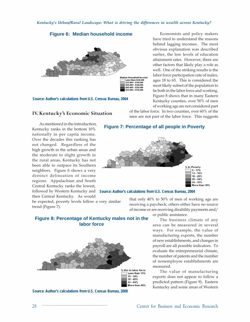
As mentioned in the introduction, Kentucky ranks in the bottom 10% nationally in per capita income. Over the decades this ranking has not changed. Regardless of the high growth in the urban areas and the moderate to slight growth in the rural areas, Kentucky has not been able to outpace its Southern neighbors. Figure 6 shows a very distinct delineation of income regions. Appalachian and South Central Kentucky ranks the lowest, followed by Western Kentucky and then Central Kentucky. As would be expected, poverty levels follow a very similar trend (Figure 7).

Economists and policy makers have tried to understand the reasons behind lagging incomes. The most obvious explanation was described earlier, the low levels of education attainment rates. However, there are other factors that likely play a role as well. One of the striking results is the labor force participation rate of males, ages 18 to 65. This is considered the most likely subset of the population to be both in the labor force and working. Figure 8 shows that in many Eastern Kentucky counties, over 50% of men of working age are not considered part

of the labor force. In two counties, over 60% of the men are not part of the labor force. This suggests

that only 40% to 50% of men of working age are receiving a paycheck; others either have no source of income or are receiving disability payments and/

or public assistance. The business climate of any

area can be measured in several ways. For example, the value of manufacturing exports, the number of new establishments, and changes in payroll are all possible indicators. To evaluate the entrepreneurial climate, the number of patents and the number of nonemployee establishments are measured.

The value of manufacturing exports does not appear to follow a predicted pattern (Figure 9). Eastern Kentucky and some areas of Western

Figure 6: Median household income


Figure 8: Percentage of Kentucky males not in the labor force


Figure 7: Percentage of all people in Poverty




Kentucky have very little if not zero manufacturing exports. Counties on the Tennessee border and the Ohio River have higher levels of exports as well as some of the urban counties. Many rural counties did not receive a single patent in 1999 (Figure 10), the most recent year of data available. It is of little surprise that the counties with higher levels of patents per capita are in the metropolitan areas where the universities and high-tech firms are located. In addition, rural counties have a smaller share of nonemployment establishments, suggesting a smaller number of entrepreneurs (Figure 11).

Figure 9: Manufacturing exports per capita

Source: Author’s calculations from Economic Census, 2002

Figure 10: Patents per capita

Source: Author’s calculations from U.S. Patents Office, 1999

Figure 11: Nonemployer Establishments Per Capita

Source: Author’s calculations from Economic Census, 2002 Nonemployer Statistics



V. Kentucky’s Quality of Life

There are other factors that indicate the satisfaction of an individual living in a particular county or region besides income-related measures. These indicators include accessibility, transportation, crime, health, and natural amenities. Figures 12 and 13 provide a brief overview of how some of these indicators vary over the state and throughout different rural regions. Commuting long distances takes time away from other activities. Figure 12 is interesting in that it has several interpretations. In the counties that surround the three major metropolitan areas, Lexington, Louisville, and Northern Kentucky, many individuals commute out of their county into an urban county. Thus we expect that fewer people would be working in their county of residence. However, once we move out to the rural counties, m a n y i n d i v i d u a l s are commuting out of their county either to work in the urban areas or commuting to surrounding counties because the jobs are not available within the i r own county . Essentially, this figure shows that there might be a differentiation

between necessity and choice. Those who live near urban count ies might have made the job choice first and then purchased a home in a surrounding county. In rural counties, residents have chosen where to live first and then m u s t c o m m u t e out of the county because of limited job selection.

Another factor contr ibut ing to

quality of life is health status. There are numerous indicators that measure health status: lack of physical activity, prevalence of obesity, smoking rates, cancer rates, access to primary care, and the percentage uninsured. Figure 13 illustrates the uninsured rates across Kentucky. High rates of uninsured can be found in Eastern and South Central Kentucky. The problems of not having health insurance are two-fold. One, individuals do not seek preventative care and only visit a health care provider after they are already ill or in an emergency situation. Second, the uninsured often visit public hospitals for non-life threatening issues and thus put a strain on hospital finances when they are unable to pay their bill.

Figure 13: Percentage of individuals without health insurance

Source: Author’s calculations from www.kentuckyhealthfacts.org, 2007

Figure 12: Percentage of individuals working within county of residence




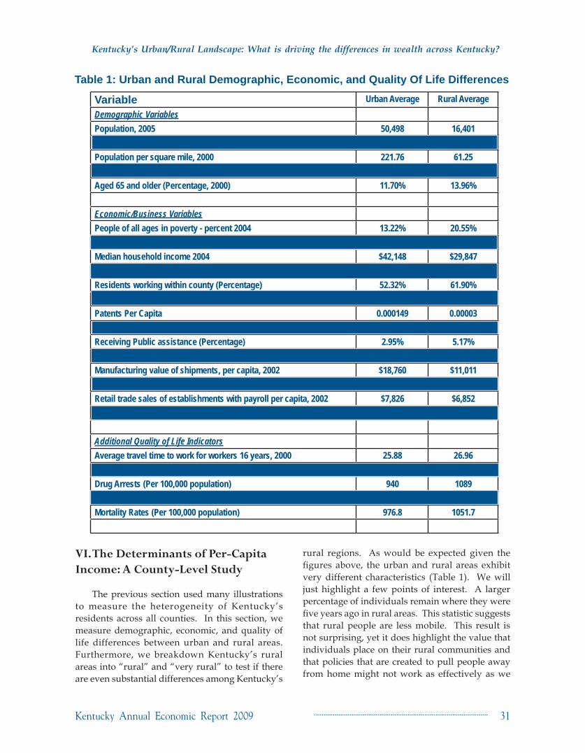
Variable Urban Average Rural AverageDemographic VariablesPopulation, 2005 50,498 16,401Population 5 years in same house, (1995-2000 Percentage) 54.47% 61.95%Population per square mile, 2000 221.76 61.25High school degree or more (Percentage, 2000) 79.72% 67.30%Aged 65 and older (Percentage, 2000) 11.70% 13.96%

Economic/Business VariablesPeople of all ages in poverty - percent 2004 13.22% 20.55%Median value of specified owner-occupied housing units, 2000 $90,403 $61,925 Median household income 2004 $42,148 $29,847 Males not in labor force (Percentage) 27.72% 39.17%Residents working within county (Percentage) 52.32% 61.90%Federal Government expenditure per capita FY, 2004 $5,873 $7,164 Patents Per Capita 0.000149 0.00003Not in labor force (Percentage) 35.70% 46.03%Receiving Public assistance (Percentage) 2.95% 5.17%Civilian labor force unemployment rate, 2006 5.50% 6.80%Manufacturing value of shipments, per capita, 2002 $18,760 $11,011 Wholesale sales of establishments with payroll, per capita, 2002 $16,096 $2,293 Retail trade sales of establishments with payroll per capita, 2002 $7,826 $6,852 Working in White Collar job (Percentage) 27.09% 25.79%

Additional Quality of Life IndicatorsAverage travel time to work for workers 16 years, 2000 25.88 26.96Uninsured Rate, 2007 (Percentage) 12.42% 15.92%Drug Arrests (Per 100,000 population) 940 1089Crime Per Capita 0.036 0.019Mortality Rates (Per 100,000 population) 976.8 1051.7

Table 1: Urban and Rural Demographic, Economic, and Quality Of Life Differences

VI. The Determinants of Per-Capita Income: A County-Level Study

The previous section used many illustrations to measure the heterogeneity of Kentucky’s residents across all counties. In this section, we measure demographic, economic, and quality of life differences between urban and rural areas. Furthermore, we breakdown Kentucky’s rural areas into “rural” and “very rural” to test if there are even substantial differences among Kentucky’s

rural regions. As would be expected given the figures above, the urban and rural areas exhibit very different characteristics (Table 1). We will just highlight a few points of interest. A larger percentage of individuals remain where they were five years ago in rural areas. This statistic suggests that rural people are less mobile. This result is not surprising, yet it does highlight the value that individuals place on their rural communities and that policies that are created to pull people away from home might not work as effectively as we



Variable Very Rural(Beale Codes 7-9)

Rural Average(Beale Codes 4-6)

Demographic VariablesPopulation, 2005 14,434 20,841Population 5 years in same house, (1995-2000 Percentage) 63.84% 57.90%Population per square mile, 2000 52.26 80.57High school degree or more (Percentage, 2000) 64.7% 72.7%Aged 65 and older (Percentage, 2000) 14.04% 13.78%

Economic/Business VariablesPeople of all ages in poverty - percent 2004 22.3% 16.8%Median value of owner-occupied housing units, 2000 $57,879 $70,614Median household income 2004 $24,609 $31,537Males not in labor force (Percentage) 42.0% 33.1%Residents working within county (Percentage) 60.1% 64.4%Federal Government expenditure per capita FY, 2004 $7,710 $6,910Patents Per Capita 0.34 1.07Not in labor force (Percentage) 48.5% 40.8%Receiving Public assistance (Percentage) 5.9% 3.6%Civilian labor force unemployment rate, 2006 7.11% 6.15%Manufacturing value of shipments, per capita, 2002 $6,852 $17,012Wholesale sales of establishments, per capita, 2002 $2,019 $2,688Retail trade sales of establishments per capita, 2002 $6,881.8 $6,870.8Working in White Collar job (Percentage) 26.9% 23.4%

Additional Quality of Life IndicatorsAverage travel time to work for workers 16 years, 2000 27.75 25.25Uninsured Rate (Percentage) 17.0% 13.6%Drug Arrests (Per 100,000 population) 1063.4 1143.9Crime Per Capita 0.016 0.026Mortality Rates (Per 100,000 population) 1063.3 1026.7

Table 2: Examining Differences Across Rural Counties

would believe. There are significantly higher rates of public assistance, federal spending, poverty, and unemployment in rural counties. In addition, while drug arrests are higher in rural areas, crime is lower.

We were also interested in examining differences among rural counties. We have seen that urban counties are quite different than rural but are there discernible differences between rural counties with rural-urban continuum codes between four and

six (rural but could be close to an urban area) and those that are between seven and nine (most rural). Table 2 provides the averages for the same variables as Table 1 but for the two different rural areas. Using a difference in means t-test with α = 0.05, those variables that were found to be significantly different between the two rural areas are in bold. There are few surprises in the results. In most instances the very rural counties are significantly more “distressed” in all three categories, particularly



Table 3: Semilog Regression ResultsDependent Variable is Log Median Household Income†

Coefficients Standard ErrorIntercept 9.4560 0.1471Demographic IndicatorsPopulation Change (%) 0.0055 0.0012Aged 65 and older (%)* -0.0053 0.0031High School Degree or more (%) 1.8723 0.1421Economic IndicatorsNot in Labor Force, male (%) -0.3746 0.1137Manufacturing Per Capita 0.0007 0.0003White Collar Worker (%) -0.2865 0.0988Quality of Life IndicatorsCommute Within County of Residence (%) -0.0024 0.0004Uninsured Population (%) -0.0088 0.0029Crime Per Capita 0.5550 0.2448R2 = 0.9464† All variables listed are statistically significant with α = .05, except for variables denoted with an asterisk which is significant at α = 0.10.

when measured with economic indicators.Successful rural economic development policy

relies on understanding the factors that influence the targeted intended outcome. In most instances, policy is created to improve the wealth of a region’s residents. Thus, in the section, we will investigate what factors influence household income at the county level. We will utilize the data in the previous section because all of these variables are expected to impact income, either directly or indirectly. The results from the regression analysis are given in Table 3. In total, there were 120 observations, one representing each county in Kentucky. The dependent variable was defined as the natural log of median household income. We will briefly interpret the results. All of the signs on the coefficients for the three significant demographic variables were as hypothesized. Population growth is typically a consequence of a region successfully attracting new residents. Individuals of working age would likely only move to an area where job prospects were promising, thus we would expect incomes to be higher in these communities. Counties with a high percentage of senior citizens are expected to have lower incomes because senior citizens are typically either not working or they are working part-time at relatively lower incomes. Of course, areas with higher educational attainments are associated with

higher incomes on average. Small positive changes in educational attainment will reap relatively large income gains.

The results for the economic indicators suggest that the higher the percentage of males not in the labor force, the lower the median household income. This result was anticipated and is believed to be a very large influence on income. Improvements in male labor-force participation rates are associated with higher incomes.

We expected that white-collar workers earn on average higher incomes than blue-collar workers and therefore we would predict that counties with a high percentage of white-collar workers would have relatively higher household incomes. The results indicated that this prediction only holds in urban areas. In rural areas, white-collar workers likely get paid below-average incomes for their profession compared to urban areas, as well as below-prevailing wages in the blue-collar professions paid to workers in rural counties. Counties with a high value of manufacturing exports have higher incomes. This result was expected for two reasons. Manufacturing plants will likely hire some share of local workers. The more valuable the produced goods, the higher the incomes the firm will be able to pay their workers. In addition, manufacturing plants might also purchase some of their inputs



locally, thus infusing the local economy with dollars generated from a valuable export business.

There were three statistically significant quality-of-life indicators: the percentage of households commuting within the county, the percentage of uninsured individuals, and crime per capita. A county with a large share of households working within their county of residence will have lower average income, all else held constant. This result appears to support the notion that out of necessity people leave their home county and commute to surrounding counties or urban areas for work; staying home results in lower incomes. Counties with high levels of uninsured populations experience lower levels of income. This variable could be a proxy for a quality-of-job variable. Lower-quality jobs are typically low paying and often do not offer health insurance. Finally, areas with higher crime will have higher incomes. This result was not as hypothesized but this variable could also be measuring other indicators that might describe positive opportunities that you might also find in an urban area, such as high growth and quality job opportunities.

VII. Conclusion

In the past, we have explored Kentucky’s standing in relation to the rest of the nation and the surrounding southern states. However, little has been done in the literature to examine how the rural and urban areas of Kentucky differ from one another. We have always known that we have at least two distinct economies, the cities of Kentucky

and the lagging rural areas. This study examines, at the county level, the differences in demographic, economic, and quality of life conditions for urban and rural areas. We further differentiate the rural areas by rural-urban continuum codes to explore possible subtle differences that might be useful in designing effective policy tools.

In addition, we also investigate the factors that are correlated with household income at the county level. This county-level study has not been done in Kentucky before, and the results reveal that effective economic development policies should target the improvement in both high school education attainment rates and male labor force participation rates. Although it is uncertain exactly how to achieve improvements in both of these variables, we can conclude that there would likely be large payoffs to the rural regions of Kentucky in terms of higher incomes.

VIII. References

Sanford, Kenneth, and Kenneth Troske (2007), “Why Is Kentucky So Poor? A Look at the Factors Affecting Cross-State Differences in Income,” 2007 Kentucky Annual Report,” 1-10.

(Endnotes)

1 Bureau of Economic Analysis, State Personal Income 2007 2 U.S. Census Bureau 2006 estimate based on 2003 ERS

Urban-Rural continuum codes. 3 U.S. Census of Agriculture, 2002

Documents

Kentucky’s Urban/Rural Landscape - University of …cedik.ca.uky.edu/files/kyruralurbanwealthdifferences.pdfKentucky’s Urban/Rural Landscape: What is driving the differences in