KALMAN FILTERS

IRINA CAZAN

Abstract. The Kalman Filter is a statistical method that involves an algorithmwhich provides an efficient recursive approach to estimatating the states of a processby minimizing the mean of the squared error. The filter is a powerful tool instatistical signal processing that allows for acurate estimations of past, present andfuture states, even with an incomplete or imprecise system model.

1. Introduction and Motivation

Rudolf Kalman is an electrical engineer noted for his co-invention of the KalmanFilter, a mathematical technique widely used in the digital computing of controlsystems, navigation systems, avionics, and outer-space vehicles. The Kalman Filterextracts a signal from a long sequence of noisy or incomplete technical measurements,usually made by electronic systems.Professor Kalman developed his theory in the late 1950s while working at the Re-

search Institute for Advanced Studies in Baltimore, Maryland. His breakthrough isdescribed in the paper ”A New Approach to Linear Filtering and Prediction Prob-lems” in 1960. [2]The Kalman filter, and its later extensions to nonlinear problems, represents one of

the most widely applied products of modern control theory. It has been used in spacevehicle navigation and control (e.g. the Apollo vehicle), radar tracking algorithms foranti-ballistic missile applications, process control, and socio-economic systems. Itspopularity in a variety of applications is due to the fact that the digital computeris effectively used in both the design phase as well as the implementation phase ofthe application. From a theoretical point of view, it brought under a common roofrelated concepts of filtering and control, and the duality between these two problems.The Kalman filter uses elements of estimation theory to obtain the best unbiased

estimator of a state of a dynamic system using previous measurement knowledge.Previous algorithms suffer from the computational limitation of using all previous in-formation to estimate the state of the system at the next time step. In contrast, theKalman filtering method makes use of the previous time step information and makesa-priori and a-posteriori predictions which are corrected using the new measurement.The prediction-correction iterations make use of Bayes’ Rule and a collection of con-cepts which will be presented in section 2. Section 3 will cover in detail the systemmodel. Section 4 contains a description of the Kalman filtering algorithm, whichwill be derived using two different approaches, followed by section 5 presenting onepossible application of the filtering method.

1

2 IRINA CAZAN

2. Preliminaries

2.1. Estimation Theory. Estimation theory is a branch of statistics used in signalprocessing that deals with methods of extracting information from noisy observations.Its goal is to estimate the values of parameters based on measured data that has arandom component. The parameters govern an underlying physical setting in such away that the values of the parameters describe the distribution of the measured data.An estimator attempts to approximate the unknown parameters using measurementsobtained from a population. A population can be defined as the set of elements withthe characteristic one wishes to understand. Because there is rarely enough time ormoney to gather information from everyone or everything in a population, the goalbecomes finding a representative sample (or subset) of that population. Estimationtheory assumes that the observations contain an information-bearing quantity, there-fore assuming that detection-based preprocessing has been performed (it is askingwhether there is something in the observations worth estimating).

Definition 2.1. (Random Variable) A random variable X is a function that assigns

a real number, X(ξ), to each outcome ξ in the sample space of a random experiment.

X : S → R. The range of the random variable is a subset of the set of all real

numbers.

Remark. The function that assigns values to each outcome is fixed and deterministic.The randomness in the observed values is due to the underlying randomness of thearguments of the function X, namely the experiment outcomes ξ. In other words,the randomness in the observed values of X is induced by the underlying randomexperiment, and we should therefore be able to compute the probabilities of theobserved values in terms of the probabilities of the underlying outcomes.

The behavior of a random variable is governed by chance, thus we can describethe behavior of a random variable in terms of probabilities. A random variable iscompletely described by telling the probability of each outcome.The most fundamental property of an random variable X is its probability distri-

bution function (PDF) FX(x), defined as

(2.1) FX(x) = P (X ≤ x)

In the above equation, FX(x) is the PDF of the random variable X, and x is anonrandom independent variable or constant. The probability density function (pdf)fx(x) is defined as the derivative of the PDF.

(2.2) fX(x) =dFX(x)

dx

One of the most commonly used pdfs of a random variable and the one that wewill be using later on in postulating the system model is the Gaussian or normaldistribution. A random variable is called Gaussian or normal if its pdf is given by

KALMAN FILTERS 3

the following equation

(2.3) fX(x) =1

σ√2π

exp [−(x− µx)2

2σ2]

The quantities in the above equation will be explained in the following definitions.Furthermore, we will drop the index for the pdf fX(x), to simplify the notation.Let X be a random variable and let g : R → R be a real-valued function defined

on the sample space of X. Define Y = g(X), that is Y is determined by evaluatingthe function g(x) at the value assumed by the random variable X. Then g(X) is alsoa random variable. The probabilities with which Y takes on various values dependon the function g(x) as well as the distribution function of X.

Remark. The density function of a random variable completely describes the behav-ior of the variable. However, associated with any random variable are constants, orparameters, which are descriptive. Knowledge of the numerical values of these param-eters gives the researcher quick insight into the nature of the variables. We considerthree such parameters: the mean µ, the variance σ

2 and the covariance Σ.

To understand the reasoning behind many statistical methods, it is necessary to be-come familiar with one general concept, namely, the idea of mathematical expectationor expected value.

Definition 2.2. (Expected Value) Let X be a real-valued random variable with density

function f(x). The expected value µ = E[X] is defined by

µ = E[X] =

� ∞

−∞xf(x)dx

provided the integral � ∞

−∞|x|f(x)dx

is finite. When used in a statistical context, the expected value of a random variable

X is referred to as its mean and is denoted by µ or µx. The mean can be thought

of as a measure of the ”center of location” in the sense that it indicates where the

”center” of the density lies.

Theorem 2.3. (Properties of the expected value) Let X and Y be real-valued random

variables and c ∈ R a scalar, then

E[X + Y ] = E[X] + E[Y ]

E[cX] = cE[X]

Definition 2.4. Let X and Y be independent real-valued continuous random variables

with finite expected values. Then we have

E[XY ] = E[X]E[Y ]

4 IRINA CAZAN

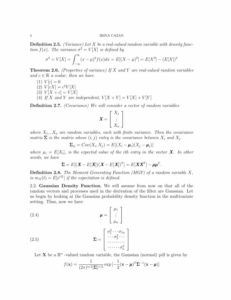
Definition 2.5. (Variance) Let X be a real-valued random variable with density func-

tion f(x). The variance σ2 = V [X] is defined by

σ2 = V [X] =

� ∞

−∞(x− µ)2f(x)dx = E[(X − µ)2] = E[X2]− (E[X])2

Theorem 2.6. (Properties of variance) If X and Y are real-valued random variables

and c ∈ R a scalar, then we have

(1) V [c] = 0(2) V [cX] = c

2V [X]

(3) V [X + c] = V [X](4) If X and Y are independent, V [X + Y ] = V [X] + V [Y ]

Definition 2.7. (Covariance) We will consider a vector of random variables

X =

X1...

Xn

where X1, , Xn are random variables, each with finite variance. Then the covariance

matrix ΣΣΣ is the matrix whose (i, j) entry is the covariance between Xi and Xj

ΣΣΣij = Cov(Xi, Xj) = E[(Xi − µµµi)(Xj − µµµj)]

where µi = E[Xi], is the expected value of the ith entry in the vector X. In other

words, we have

ΣΣΣ = E[(X− E[X])(X− E[X])T ] = E[XXT ]− µµµµµµT.

Definition 2.8. The Moment Generating Function (MGF) of a random variable X,

is mX(t) = E[etX ] if the expectation is defined.

2.2. Gaussian Density Function. We will assume from now on that all of therandom vectors and processes used in the derivation of the filter are Gaussian. Letus begin by looking at the Gaussian probability density function in the multivariatesetting. Thus, now we have

µµµ =

µ1...µn

(2.4)

ΣΣΣ =

σ21 · · · σ1n

· · · σ22 · · ·

· · · · · · · · ·· · · · · · σ2

n

(2.5)

Let X be a Rn -valued random variable, the Gaussian (normal) pdf is given by

f(x) =1

(2π)n/2|ΣΣΣ|1/2 exp [−1

2(x− µµµ)TΣΣΣ−1(x− µµµ)]

KALMAN FILTERS 5

where � ∞

−∞· · ·

� ∞

−∞f(x)dx1 · · · dxn = 1,

E[X] = µµµ = mean value of vector,

E[(X− µµµ)(X− µµµ)T ] = ΣΣΣ = covariance matrix of vector,

Also, |ΣΣΣ| is the determinant of ΣΣΣ, ΣΣΣ−1 is the matrix inverse of ΣΣΣ. We can observethat f(X) is completely characterized via two parameters - mean and covariancematrix.It is important to note that adding two (or more) Gaussian random vectors produces

a Gaussian random vector with mean equal to the sum of means and variance equalto the sum of variances of the two random vectors. Expressed more formally,

Theorem 2.9. Let X and Y be two normal (Gaussian) independent random vectors.

Then X + Y is also normally distributed. In particular, if X ∼ N(µxµxµx,ΣxΣxΣx) (X has

a normal distribution) and Y ∼ N(µµµy,ΣyΣyΣy) and X and Y are independent, then

Z = X+Y ∼ N(µxµxµx + µyµyµy,ΣxΣxΣx +ΣyΣyΣy).

Proof. The moment generating function of the sum of two independent random vari-ables X and Y is just the product of the two separate moment generating functions:

(2.6) mX+Y (t) = E[et(X+Y )] = E[etX ]E[etY ] = mX(t)mY (t)

Remark. For a random variable X ∼ N(µ, σ2), we can determine the moment gener-ating function to be

(2.7) mX(t) =

� ∞

−∞

etx

σ√2π

e− (x−µ)2

2σ2 dx = eµt +

σ2t2

2

Therefore, using this in the above equation, we obtain

(2.8) mX+Y (t) = mX(t)mX(t) = etµx−

σ2xt2

2 etµx−

σ2yt2

2 = et(µx+µy)−

(σ2x+σ2

y)t2

2

This is the moment generating function of the normal distribution with expectedvalue µx+µy and variance σ2

x+σ2y . Recall that two distinct distributions cannot both

have the same moment generating function, hence the distribution of X +Y must bethis normal distribution.Let

XXX =

X1...

Xn

and

YYY =

Y1...Yn

6 IRINA CAZAN

Then

X + YX + YX + Y =

X1 + Y1

...Xn + Yn

Since by taking the expected value of a vector of random variables we take theexpected value of each of its components, we obtain

E[X + YX + YX + Y ] =

E[X1 + Y1]

...E[Xn + Yn]

=

E[X1] + E[Y1]

...E[Xn] + E[Yn]

=

µx,1 + µy,1

...µx,n + µy,n

= µxµxµx + µyµyµy

ΣXXX+YYYΣXXX+YYYΣXXX+YYY = E[(XXX + YYY )(XXX + YYY )T ]− (µXµXµX + µYµYµY )(µXµXµX + µYµYµY )T

= E[(X1 + Y1)2 + · · ·+ (Xn + Yn)

2]− (µXµXµX + µYµYµY )(µXµXµX + µYµYµY )T

= E[(X21 + · · ·+X

2n) + (Y 2

1 + · · ·+ Y2n )] + 2E[X1Y1 + · · ·+XnYn]

− ((µx,1 + µy, 1)2 + · · ·+ (µx,n + µy, n)2)

= E[(X21 + · · ·+X

2n)] + E[(Y 2

1 + · · ·+ Y2n )] + 2E[X1Y1 + · · ·+XnYn]

− ((µ2x,1 + · · ·+ µ

2x,n) + (µ2

y,1 + · · ·+ µ2y,n) + 2(µx,1µy,1 + · · ·+ µx,nµy,n))

= E[(X21 + · · ·+X

2n)]− (µ2

x,1 + · · ·+ µ2x,n) + E[(Y 2

1 + · · ·+ Y2n )]− (µ2

y,1 + · · ·+ µ2y,n)

= ΣXΣXΣX +ΣYΣYΣY

This completes our proof.�

2.3. Random Processes and the Markov Property. A random process is a col-lection of continuous-valued random variables indexed by a continuous-valued param-eter x(t), t0 ≤ t ≤ tf . Since the state of continuous dynamic processes that occur innatural or man-made systems can never be known exactly, since they are subject todisturbances, these processes are random processes. To have a complete descriptionof such a random process, we would need to know all possible joint density functions

f [x(t1), x(t2), . . . , x(tN)]

for all t’s in the interval (t0, tf ), where the index of t runs from 1 to ∞. It is notfeasible to supply and use such a large amount of information for a given process.Most common processes have the property of being Markovian, with a Markov processbeing completely specified by giving the joint density function

f [x(t), x(τ)] = f [x(t)|x(τ)]f [x(τ)]for all t, τ in the interval (t0, tf ). [4]

KALMAN FILTERS 7

Definition 2.10. (Purely Random Process or White Noise) In the case that p[x(t)|x(τ)] =p[x(t)] for all t and τ in (t0, tf ) the process is called a purely random process or white

noise. If the process involves an outside disturbance f(t), with p[f(t)|f(τ)] ∼= p[f(t)]for |t − τ | ≥ T , with T much smaller that the average response time of the system

analyzed, then f(t) may be considered as white noise relative to the system. [4]

Gauss-Markov Random Process. A Gauss-Markov random process is a Markovrandom process with the added restriction that p[x(τ)] and p[x(t)|x(τ)] are Gauss-ian density functions for all t, τ in the interval (t0, tf ). Therefore, the densityfunction p[x(t)] of a Gauss-Markov process is completely described by giving themean or expected value vector µx(t) = E[x(t)] and the covariance matrix Covx(t) =E[x(t)− µx(t)][x(t)− µx(t)]T . The importance of this type of process flows from thefact that most natural and man-made dynamic processes may be approximated ratheraccurately using Gauss-Markov processes. [4] Furthermore, it is very common to ap-proximate a non-Gaussian Markov process by a Gauss-Markov random process be-cause there is usually limited statistical knowledge available about the actual process.[4]

2.4. Least Squares Estimator and the Gauss - Markov Theorem.Least squares estimation (LSE) can be used whenever the probabilistic information

about the data is not given. The approach here is to assume a system model (ratherthan probabilistic assumptions about the data) and achieve a design goal assumingthis model. In order to do so, we will use a linear regression model to execute theestimation.

Definition 2.11. Given a data set {Yi, Xi1, . . . , Xim}ni=1, a linear regression model

assumes that the relationship between the dependent variable Yi and the m-vector of

input random variables is linear. This relationship is modeled through a disturbance

term �i, an unobserved random variable that adds noise to the linear relationship

between the dependent variable and regressors. Thus the model takes the form

(2.9) Yi = β1Xi1 + · · ·+ βmXim + �i = XTi β + �i i=1, . . . ,n

so that XTi β is the inner product between vectors Xi and β. This can also be written

in matrix form as

(2.10) Y = XTβββ + ���

where

Y =

Y1...

Yn

,X =

X

T1...

XTn

=

X11 · · ·X1m

X21 · · ·X2m.... . .

...

Xn1 · · ·Xnm

,βββ =

β1...

βm

, ��� =

�1...

�n

8 IRINA CAZAN

In concise form, the Gauss - Markov theorem states that in a linear regression modelin which the errors have expectation zero, are uncorrelated and have equal variances,the best linear unbiased estimator (BLUE) of the coefficients is given by the ordinaryleast squares estimator. ”Best” means giving the minimum mean squared error ofthe estimate. [8]More precisely,

Theorem 2.12. (Gauss-Markov) Assuming the following linear regression model

(2.11) Y = XTβββ + ���

where βββ is a vector of non-random unobservable parameters, Xij are non-random and

observable vectors, ��� is a vector of random variables, therefore the Y’s are random

vectors. If the following conditions are met:

(1) E[�i] = 0, V [�i] = σ2and Cov(�i, �j) = 0 for all i �= j.

(2) βββ is an estimator of βββ. We say that the estimator is unbiased if the following

relationship holds: E[βββ] = βββ.

(3) Let�m

j=1 λjβj be any linear combination of the coefficients, then the mean

squared error of the estimation is E

��mj=1 λj(βj − βj)

�.

Then the BLUE of βββ is the estimator with the minimum mean squared error for

every linear combination parameters. The ordinary least squares estimator is the

function:

βββ = (XTX)−1XTY of X and Y that minimizes the sum squares of residuals :n�

i=1

(Yi − Yi)2 =

n�

i=1

(Yi −K�

j=1

βjYij)2

Hence, the ordinary least squares estimator is a BLUE.

We will skip the proof of the theorem here since it is not needed for our purposes.

Conditional expectations will play a crucial role in deriving the recursive LSE andin obtaining the Kalman filter. The calculus of conditional expectations is used in thecontext of a simple regression model in which a regression relationship is postulatedin which the unknown parameters are regarded as fixed quantities. The next fewderivations are meant to present some essential relationships within the underlyingtheoretical regression relationship. These will prove necessary in deriving the KalmanFilter algorithm in the next sections.Let X and Y be random vectors with a joint distribution completely characterized

by first and second order moments. We can define the second order moments of X

KALMAN FILTERS 9

and Y:

V [X] = E[XXT ]− E[X]E[XT ](2.12)

V [Y] = E[YYT ]− E[Y]E[YT ](2.13)

Cov(Y,X) = E[YXT ]− E[Y]E[XT ](2.14)

Let the conditional expectation of Y given X be a linear functional of X:

(2.15) E[Y|X] = ααα +BTX

The goal is to find vector ααα and matrix B in terms of the second order momentsdescribed above. First, multiply the conditional expectation by the marginal densityfunction of X and integrate with respect to X to get E[E[Y|X]] = E[Y]Using this on the above conditional expectation we obtain E[Y] = ααα + BT

E[X]and the following expression for ααα:

(2.16) ααα = E[Y]− BTE[X]

Second, we will multiply E[Y|X] by XT and by the marginal density function of Xand take its expectation

(2.17) E[YXT ] = αααE[X] +BTE[XXT ]

Multiplying E[Y] = ααα +BTE[X] by E[XT ] gives us

(2.18) E[Y]E[XT ] = αααE[X] +BTE[X]E[XT ]

Subtracting equation (2.12) from (2.13) and using the definitions for the second ordermoments in (2.10), we have

(2.19) Cov(Y,X) = BTCov(X) or BT = Cov(Y,X)Cov

−1(X)

Substituting the derived expressions for ααα, (2.12), and for BT , (2.14), into thedefinition for E[Y|X], we obtain E[Y|X] = ααα +BTX, or

(2.20) E[Y|X] = E[Y] + Cov(Y,X)Cov−1(X)(X− E[X])

Below is a summary of our findings and other equations which can be derivedsimilarly:

E[Y|X] = E[Y] + Cov(Y,X)Cov−1(X)(X− E[X])(2.21)

Cov(Y|X) = Cov(Y)− Cov(Y,X)Cov−1(X)Cov(X,Y)(2.22)

E[E[Y|X]] = E[Y](2.23)

Cov(E[Y|X]) = Cov(Y,X)Cov−1(X)Cov(X,Y)(2.24)

Cov(Y) = Cov(Y,X) + Cov(E[Y|X])(2.25)

Cov(Y− E[Y|X],X) = 0(2.26)

These will later be used in order to determine the recursive algorithm for Kalmanfiltering.

10 IRINA CAZAN

3. The Model

To begin deriving a model and solving the filtering problem, it is necessary to under-stand what is our goal and what is the information available from the instruments orsensors used to detect the desired signal. We want to estimate the state of the sys-tem, X, which is a random vector containing n different system states, and we haveavailable a set of measurements X, which is a random vector composed of m mea-surements. State X is a random variable and belongs to the following time-controlledprocess governed by the linear stochastic difference equation:

(3.1) Xk = aXk−1 + buk−1 +Wk−1

and the sensors have the following sensing model:

(3.2) Zk = hXk +Vk

where Wk and Vk are the process and measurement noise, respectively, which arezero-mean white-Gaussian random processes independent of each other: W ∼ N(0,Q)and V ∼ N(0,R), where Q and R covariance matrices defined as follows:

Q = E[WWT ],

R = E[VVT ].

The n× n matrix a relates state X at time step k − 1 to the state at time step k,the n× l matrix b relates the optional control input u ∈ Rl to state X, and the m× n

matrix h relates state Xk to measurement Zk. The above matrices are assumed to beconstant for the simplicity of the derivation. In practice, they might change at eachtime step. [1]In order to proceed with the derivation, it is necessary to introduce some notation

that will be heavily used later on. The following definitions make use of Bayes’ Rule.The essence of the Bayesian approach is to provide a mathematical rule explaininghow one should change the existing beliefs in the light of new evidence. In other words,it allows scientists to combine new data with their existing knowledge. The processinvolves a prediction-correction algorithm: one makes an assumption (prediction)about the behavior of the system at the next time step (a priori estimate) and adjustsit (a posteriori estimate) using data from sensors or measuring instruments as soonas it becomes available (correction). Therefore, we define

KALMAN FILTERS 11

X−k ∈ Rn(3.3)

Xk ∈ Rn(3.4)

e−k = Xk − X−k(3.5)

ek = Xk − Xk(3.6)

ΣΣΣ−k = E[e−k (e

−k )

T ](3.7)

ΣΣΣk = E[ekeTk ](3.8)

where X−k is the a - priori state estimate at step k (which means that we know the

process prior to step k), Xk is the a - posteriori state estimate at step k (which meansthat we know measurement Zk), e

−k is the a - priori estimate error, ek is the a -

posteriori estimate error, ΣΣΣ−k is the a - priori estimate error covariance matrix and ΣΣΣk

is the a - posteriori estimate error covariance matrix.We want to find an equation that computes an a posteriori state estimate Xk as a

linear combination of an a priori estimate X−k and a weighted difference between an

actual measurement Zk and a measurement prediction hX−k .

(3.9) Xk = X−k +Kk(Zk − hX

−k )

In equation (3.9) there are two quantities playing a significant role: Zk − hX−k is

called the measurement innovation or the residual and Kk is a n ×m matrix calledthe Kalman gain.We now need to formulate an estimation algorithm such that the following statis-

tical conditions hold:

(1) The expected value of the state estimate is equal to the expected value of thetrue state. That is,on average,the estimate of the state will equal the truestate.

(2) We want an estimation algorithm that minimizes the expected value of thesquare of the estimation error. That is,on average,the algorithm gives thesmallest possible estimation error.

In order to do so, we need to identify the optimal value for the Kalman gain,Kk. The above conditions translate into the following steps that need to be taken.First, we will take the expected value of the a posteriori error covariance and observewhether the estimator is biased. Then we will analyze the variances of the estimationerrors in order to determine whether the Kalman gain computed by the error varianceminimization process is optimal.

Theorem 3.1. The optimal value of the Kalman gain matrix (the value which mini-

mizes error covariance or achieves the best estimate) is

(3.10) Kk = ΣΣΣ−k h

T (hΣΣΣ−k h

T +R)−1

12 IRINA CAZAN

Proof. The main steps of the derivation are presented here, with the complete equa-tions included in the appendix. Consider the dynamic process model and sensingmodel as stated in the beginning of the section with ek = Xk − Xk the a posterioriestimate error. Let’s begin by looking at the mean of this error by taking its expectedvalue.

E[ek] = E[Xk − Xk] = E[(I−Kkh)e−k −KkVk].

Remark. Since Kk and h are constant at each time step and we are aiming to derivethe expression for Kk, we know that

E[Kk] = Kk

E[h] = h

E[KTk ] = KT

k

E[hT ] = hT

Given the above observation, we can now rewrite the mean of the a posteriori errorcovariance as follows

E[ek] = (I−Kkh)E[e−k ]−KkE[Vk].

Therefore, if E[Vk] = 0 and E[e−k ] = 0, then E[ek] = 0. This means that ifthe measurement noise is zero-mean for all k (which we know to be true because ofthe system model), and the initial estimate of the system state is set equal to itsexpected value, X0 = E[X0], then the expected value of Xk will be equal to Xk forall k. Because of this, the estimator of the system state is unbiased, a property whichholds regardless of the value of the gain matrix. Thus, the first requirement that wehave outlined above is satisfied.Keep in mind that the goal is to determine the optimal value of the Kalman gain

matrix. The optimality criterion used is to minimize the aggregate variance of theestimation errors at time k. Let Mk be the aggregate variance of the estimation errorsat time k. Then

Mk = E[||Xk − Xk||2] = E[eTk ek]

= E[tr(ekeTk )] = tr(E[eke

Tk ]) = tr(ΣΣΣk)

where tr is the trace operator and ΣΣΣk is the a posteriori estimate error. Let us nowget an expression for ekeTk , take its expected value and finally compute its trace. Thederivations are below.Step 1: First, we will derive an expression for ekeTk .

ekeTk = ((I−Kkh)e

−k −KkVk)((I−Kkh)e

−k −KkVk)

T

= (I−Kkh)e−k e

−Tk (I−Kkh)

T − (I−Kkh)e−k V

TkK

Tk

−KkVke−Tk (I−Kkh)

T +KkVkVTkK

Tk

KALMAN FILTERS 13

Step 2: Second, we will take the expected value of ekeTk , or E[ekeTk ].

E[ekeTk ] = E[I−Kkh]ΣΣΣ

−k E[(I−Kkh)

T ]− E[(I−Kkh)e−k V

TkK

Tk ]

− E[KkVke−Tk (I−Kkh)

T ] + E[KkVkVTkK

Tk ]

Remark. E[Vk] = 0, E[VTk ] = 0 and Vk is independent of the other terms in the

expectation it appears in (thus its expectation can be factored out), because itwas defined as a measurement noise, which is white Gaussian noise. Thus, E[(I −Kh)e−k V

TkK

T ] = 0 = E[KVke−Tk (I−Kh)T ].

Therefore, ΣΣΣk = E[ekeTk ] becomes:

E[ekeTk ] = E[I−Kkh]ΣΣΣ

−k E[(I−Kkh)

T ] + E[KVkVTkK

Tk ]

Step 3: In order to minimize matrix ΣΣΣk, we need to minimize its trace. Therefore,the goal now is to minimize tr(E[ekeTk ]). We will do this by taking the derivative ofthe trace with respect to Kk. To this effect, replace Kk with Kk + tU , where t is ascalar and U is a direction matrix, and take the derivative with respect to t at t = 0.Hence we get the following expression

Mk = tr((I−Kkh)ΣΣΣ−k (I−Kkh)

T − t((IΣΣΣ−k h

TU

T + UhΣ−k (I−Kkh)

T )

+ t2(. . .) +KkRKT

k + tKkRUT + tURKT

k + t2(. . .))

Now take the derivative with respect to t at t = 0 and set equal to 0. Only thecoefficients of the linear terms will remain.

∂Mk

∂Kk=− tr((I−Kh)ΣΣΣ−

k (Uh)T )− tr(UhΣΣΣ−k (I−Kh)T

+ tr(KRUT ) + tr(URKT ) = 0

Since tr(AT ) = tr(A) because diagonals are preserved, notice that tr(UTK) =tr((KT

U)T ) = tr(KTU). Also, by the same reasoning, tr(UhΣΣΣ−

k (I − Kh)T ) =tr((IKh)ΣΣΣ−

k (UH)T ). Thus, the above expression becomes:

∂Mk

∂Kk= tr(−UhΣΣΣ−

k (I−Kh)T +KTUR) = 0

Since R = E[VVT ] andΣΣΣ−k = E[e−k e

−Tk ], they are both symmetric matrices. Hence,

RT = R and ΣΣΣ−Tk = ΣΣΣ−

k . Also, for symmetric matrix R and matrices A,B,C, thefollowing are true: tr(RA) = tr((AT

R)T ) = tr(ATR) = tr(RA

T ) and tr(ABC) =tr(CAB) = tr(BCA).Using these, we get

∂Mk

∂Kk= tr(−hΣ−

k (I−Kh)T +RKT )U) = 0

14 IRINA CAZAN

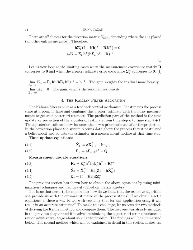
There are n2 choices for the direction matrix Un×n, depending where the 1 is placed(all other entries are zeros). Therefore:

− hΣΣΣ−k (I−Kh)T +RKT ) = 0

⇔K = ΣΣΣ−k h

T (hΣΣΣ−k h

T +R)−1

�Let us now look at the limiting cases when the measurement covariance matrix R

converges to 0 and when the a priori estimate error covariance ΣΣΣ−k converges to 0. [1]

limRk→0

Kk = ΣΣΣ−k h

T (hΣΣΣ−k h

T )−1 = h−1 The gain weights the residual more heavily

limΣΣΣ−

k →0Kk = 0 The gain weights the residual less heavily

4. The Kalman Filter Algorithm

The Kalman filter is built as a feedback control mechanism. It estimates the processstate at a point in time and combines this a priori estimate with the noisy measure-ments to get an a posteriori estimate. The prediction part of the method is the timeupdate, or projection of the a posteriori estimate from time step k to time step k+1.The a posteriori estimate now becomes the new a priori estimate after the projection.In the correction phase the system receives data about the process that it postulateda belief about and adjusts the estimator in a measurement update at that time step.Time update equations:

X−k = a ˆXk−1 + buk−1(4.1)

ΣΣΣ−k = aΣΣΣk−1a

T +Q(4.2)

Measurement update equations:

Kk = ΣΣΣ−k h

T (hΣΣΣ−k h

T +R)−1(4.3)

Xk = X−k +Kk(Zk − hX

−k )(4.4)

ΣΣΣk = (I−Kkh)ΣΣΣ−k(4.5)

The previous section has shown how to obtain the above equations by using mini-mization techniques and had heavily relied on matrix algebra.The issue that needs to be explored is: how do we know that the recursive algorithm

will provide us with the optimal estimator of the process states? If we obtain a set aequations, is there a way to tell with certainty that for any application using it willresult in an accurate estimator? To tackle this challenge, let us consider two methodsof deriving the Kalman method and compare them. The first one was already includedin the previous chapter and it involved minimizing the a posteriori error covariance, arather intuitive way to go about solving the problem. The findings will be summarizedbelow. The second method which will be explained in detail in this section makes use

KALMAN FILTERS 15

of recursive least square estimation and will hinge on the Gauss - Markov Theorempresented in the Preliminaries section. According to the theorem, the recursive LSEmethod will allow us to find the best linear unbiased estimator (BLUE) every timeif the underlying assumptions are satisfied. After the derivation is complete we willcompare the methods and draw our conclusions.We are given the following regression model, which is the sensing model for the

dynamic process assumed in section 3:

Zk = hXk +Vk

where E[Vk] = 0, V [Vk] = R, and Cov(Vk,Vl) = 0 for k �= l. We also know thatthe system states, the Xs are related in the following way:

Xk = aXk−1 + buk−1 +Wk−1

with Xk a linear estimator of Xk. Since the assumptions of the Gauss - MarkovTheorem are satisfied, we know that the estimators for Xk at each time step will beBLUEs.Now, given a set of observations at time k, Zk, we want to derive the a posteriori

estimates Xk = E[Xk|Zk] and Σk = Cov(Xk|Zk) from the a priori estimates X−k and

ΣΣΣ−k . To begin with, let X be Zk and Y be Xk in (2.17) and get:

(4.6) E[Xk|Zk] = E[Xk|Zk−1]+Cov(Xk,Zk|Zk−1)Cov−1(Zk|Zk−1)(Zk−E[Zk|Zk−1])

Following E[Xk|Zk−1], there are three quantities that we are particularly interestedin: the covariance, the variance-covariance, and the error from predicting Zk usingthe available observations or measurements.

Cov(Xk,Zk|Zk−1) = E[(Xk − X−k )Z

Tk ] = E[(Xk − X

−k )(hXk)

T ] = ΣΣΣ−k h(4.7)

Cov(Zk|Zk−1) = Cov(h(Xk − X−k ) + Cov(Vk) = h SigmaSigmaSigma

−k h

T +R(4.8)

Zk − E[Zk|Zk−1] = Zk − hX−k := Fk(4.9)

Using these derivations, we can return to equation (2.21) and get

(4.10) Xk = X−k +ΣΣΣ−

k hT (h SigmaSigmaSigma

−k h

T +R)−1)(Zk − hX−k )

Similarly, using equation (2.16) we have that

Cov(Xk|Zk) = Cov(Xk|Zk−1) = Cov(Xk,Zk|Zk−1)Cov−1(Zk,Xk|Zk−1)(4.11)

ΣΣΣk = ΣΣΣ−k −ΣΣΣ−

k hT (hΣΣΣ−

k +R)−1hΣΣΣ−k(4.12)

16 IRINA CAZAN

Summing up, we now have the measurement update equations to run the recursiveleast-squares algorithm.

Fk = Zk − hX−k Residual(4.13)

Sk = hΣΣΣ−k h

T +R Error covariance(4.14)

Kk = ΣΣΣ−k h

TSk Filter gain(4.15)

Xk = X−k +KkFk Parameter estimate(4.16)

ΣΣΣk = (I−KkhT )ΣΣΣ−

k Estimate covariance(4.17)

The time update is performed as stated in the previous model, since it does notdepend on the derivation method. The time update only involves the forward projec-tion of the a priori estimate and error covariance using the system model. Therefore,we now have the full set of prediction-correction equations:

Time update/ Prediction phase X−k = aXk−1 + buk−1(4.18)

ΣΣΣ−k = aΣΣΣk−1a

T +Q(4.19)

Measurement update/ Correction phase Kk = ΣΣΣ−k h

TSk(4.20)

Xk = X−k +KkFk(4.21)

ΣΣΣk = (I−KkhT )ΣΣΣ−

k(4.22)

The results obtained by the two optimization methods used in the last two sectionsto obtain the Kalman gain for the best state estimator coincide. Therefore, theKalman filter algorithm derived by the two methods is optimal under the modelassumptions. In the first method I approached the problem by minimizing the aposteriori error covariance using the first order condition of setting the derivativeequal to 0 and solving for the gain. The second method relies heavily on the Gauss- Markov Theorem assumptions to conclude that the estimator obtained using thecomputed Kalman gain is the best linear unbiased estimator. Because the same resulthas been reached using two very different methods points out that, given the assumedmodel, we have come up with the best estimator for the system states at each timestep.

Below is a representation of the predictor-corrector mechanism that constitutesthe Kalman filter. Each time an input passes through a box, it gets multiplied withthe amount written inside. Inputs are added/subtracted at each node, accordingto indications. All notation appearing in the figure have been defined in the modelsection, and T represents the time delay from one time step to another.

KALMAN FILTERS 17

The top part in the dashed box simply represents the system model characterizedby equations (3.8) and (3.9). The whole picture shows the time and measurementupdates that happen at each iteration.

5. Application: Estimate the Position and Velocity of a MovingVehicle

The Kalman filter is a tool that can estimate the parameters of a wide range ofprocesses. From the statistical point of view, a Kalman filter estimates the states ofa linear system. The Kalman filter is not only an excellent practical tool, but it istheoretically attractive as well because, as we have shown in section 3, it minimizesthe variance of the estimation error. This section will present the use of the filter tosolve a vehicle navigation problem. In order to control the position of an automatedvehicle, we must first have a reliable estimate of the vehicle’s present position. Kalmanfiltering provides a tool for obtaining the best linear unbiased estimate.Suppose we want to model a vehicle driving in a straight line. The state consists of

the vehicle position p and velocity v. The input u is the commanded acceleration andthe output z is the measured position. Suppose we are able to change the accelerationand measure the position every T seconds. In this case, the position p and the velocityv will be governed by the following equations:

pk+1 = pk + Tvk +1

2T

2uk(5.1)

vk+1 = vk + Tuk(5.2)

However, the previous equations do not give a precise value for pk+1 or for vk+1:the position and velocity will be perturbed by noise due to wind, road conditions,

18 IRINA CAZAN

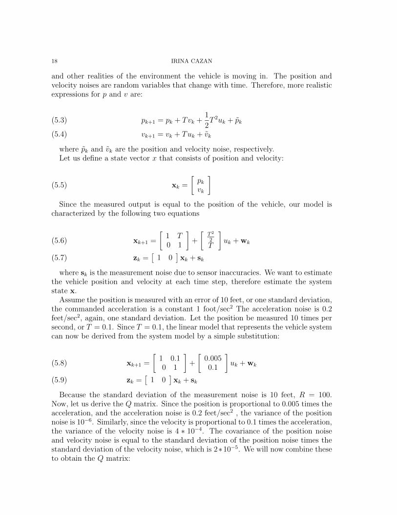
and other realities of the environment the vehicle is moving in. The position andvelocity noises are random variables that change with time. Therefore, more realisticexpressions for p and v are:

pk+1 = pk + Tvk +1

2T

2uk + pk(5.3)

vk+1 = vk + Tuk + vk(5.4)

where pk and vk are the position and velocity noise, respectively.Let us define a state vector x that consists of position and velocity:

(5.5) xk =

�pk

vk

�

Since the measured output is equal to the position of the vehicle, our model ischaracterized by the following two equations

xk+1 =

�1 T

0 1

�+

�T 2

2T

�uk +wk(5.6)

zk =�1 0

�xk + sk(5.7)

where sk is the measurement noise due to sensor inaccuracies. We want to estimatethe vehicle position and velocity at each time step, therefore estimate the systemstate x.Assume the position is measured with an error of 10 feet, or one standard deviation,

the commanded acceleration is a constant 1 foot/sec2 The acceleration noise is 0.2feet/sec2, again, one standard deviation. Let the position be measured 10 times persecond, or T = 0.1. Since T = 0.1, the linear model that represents the vehicle systemcan now be derived from the system model by a simple substitution:

xk+1 =

�1 0.10 1

�+

�0.0050.1

�uk +wk(5.8)

zk =�1 0

�xk + sk(5.9)

Because the standard deviation of the measurement noise is 10 feet, R = 100.Now, let us derive the Q matrix. Since the position is proportional to 0.005 times theacceleration, and the acceleration noise is 0.2 feet/sec2 , the variance of the positionnoise is 10−6. Similarly, since the velocity is proportional to 0.1 times the acceleration,the variance of the velocity noise is 4 ∗ 10−4. The covariance of the position noiseand velocity noise is equal to the standard deviation of the position noise times thestandard deviation of the velocity noise, which is 2∗10−5. We will now combine theseto obtain the Q matrix:

KALMAN FILTERS 19

(5.10) Q =

�10−6 2 ∗ 10−5

2 ∗ 10−5 4 ∗ 10−4

�

We will work with the following initial conditions: x0 as initial estimate of positionand velocity and Σ0) as the uncertainty in the initial estimate. Running the Kalmanfilter equations using a MATLAB routine, the following results were obtained:

20 IRINA CAZAN

Figure 1 shows the true position of the vehicle, the measured position, and theestimated position. The two smooth curves are the true position and the estimatedposition, and they almost coincide. The noisy curve is the measured position. Figure2 shows the error between the true position and the measured position, and the errorbetween the true position and the Kalman filtered estimated position. Figure 3 showsthe advantage that we get from the Kalman filter: since the vehicle velocity is partof the state x, we get a velocity estimate along with the position estimate. Figure 4shows the error between the true velocity and the Kalman filtered estimated velocity.

KALMAN FILTERS 21

Acknowledgements

I would like to thank Professors Liam O’Brian and Andreas Malmendier for theirsupervision and support.

References

[1] G. Welch, G. Bishop, An Introduction to the Kalman Filter, Department of ComputerScience, University of North Carolina at Chapel Hill, TR 95-041.

[2] R.E. Kalman, A New Approach to Linear Filtering and Prediction Problems, Transaction ofthe ASME - Journal of Basic Engineering, pp. 35-45 (March 1960).

[3] H.W. Sorenson, Least Squares Estimation: from Gauss to Kalman, IEEE Spectrum, vol. 7,pp. 63-68, July 1970.

[4] A. Bryson, Y.-C Ho, Applied Optimal Control: Optimization, Estimation, and Control[5] S. M. Kay, Fundamentals of Statistical Signal Processing: Estimation Theory, Prentice-Hall,

1993[6] P. Zarchan, H. Musoff, Fundamentals of Kalman Filtering: A Practical Approach, 3rd Edi-

tion, 2009[7] G. Casella, R. Berger, Statistical Inference, Second Edition, Thomson Learning, 2001[8] D.S.G. Pollock, The Kalman Filter etc., 2000

22 IRINA CAZAN

Appendix

Kalman Gain Derivation

E[ek] = E[Xk − Xk] = E[Xk − X−k −K(Zk − hX

−k )]

= E[Xk − (I−Kkh)X−k −KkZk]

= E[Xk − (I−Kkh)X−k −Kk(hXk +Vk)]

= E[(I−Kkh)Xk − (I−Kkh)X−k −KkVk]

= E[(I−Kkh)(Xk − X−k )−KkVk]

= E[(I−Kkh)e−k −KkVk].

E[ek] = (I−Kkh)E[e−k ]−KkE[Vk].

Mk = E[||Xk − Xk||2] = E[eTk ek]

= E[tr(ekeTk )] = tr(E[eke

Tk ]) = tr(ΣΣΣk)

Step 1:

ekeTk = ((I−Kkh)e

−k −KkVk)((I−Kkh)e

−k −KkVk)

T

= ((I−Kkh)e−k −KkVk)(e

−Tk (I−Kkh)

T − vTk K

Tk )

= (I−Kkh)e−k e

−Tk (I−Kkh)

T − (I−Kkh)e−k V

TkK

Tk

−KkVke−Tk (I−Kkh)

T +KkVkVTkK

Tk

Step 2:

E[ekeTk ] = E[I−Kkh]ΣΣΣ

−k E[(I−Kkh)

T ]− E[(I−Kkh)e−k V

TkK

Tk ]

− E[KkVke−Tk (I−Kkh)

T ] + E[KkVkVTkK

Tk ]

Therefore, ΣΣΣk = E[ekeTk ] becomes:

E[ekeTk ] = E[I−Kkh]ΣΣΣ

−k E[(I−Kkh)

T ] + E[KVkVTkK

Tk ]

Step 3: Minimize tr(E[ekeTk ]). We will do this by taking the derivative of the tracewith respect to Kk. To this effect, replace Kk with Kk + tU , where t is a scalar andU is a direction matrix, and take the derivative with respect to t at t = 0.

KALMAN FILTERS 23

Mk = tr((I− (Kk + tU)h)Σ−k (I− (Kk + tU)h)T + (Kk + tU)R(Kk + tU)T )

= tr((I−Kkh− tUh)Σ−k (I−Kkh− tUh)T + (Kk + tU)R(KT

k + tUT ))

= tr((I−Kkh)Σ−k − tUhΣ−

k )((I−Kkh)T − (thT

UT )) + (KkR+ tUR)(KT

k + tUT )

= tr((I−Kkh)ΣΣΣ−k (I−Kkh)

T − t((IΣΣΣ−k h

TU

T + UhΣ−k (I−Kkh)

T )

+ t2(. . .) +KkRKT

k + tKkRUT + tURKT

k + t2(. . .))

Now take the derivative with respect to t at t = 0 and set equal to 0. Only thecoefficients of the linear terms will remain.

∂Mk

∂Kk=− tr((I−Kh)ΣΣΣ−

k (Uh)T )− tr(UhΣΣΣ−k (I−Kh)T

+ tr(KRUT ) + tr(URKT ) = 0

∂Mk

∂Kk= −2tr(UhΣ−

k (IKh)T ) + 2tr(KTUR) = 0

⇔∂Mk

∂Kk= tr(−UhΣΣΣ−

k (I−Kh)T +KTUR) = 0

∂Mk

∂Kk= tr(−hΣ−

k (I−Kh)TU +RKTU) = 0

⇔∂Mk

∂Kk= tr(−hΣ−

k (I−Kh)T +RKT )U) = 0

There are n2 choices for the direction matrix Un×n, depending where the 1 is placed(all other entries are zeros). Therefore:

− hΣΣΣ−k (I−Kh)T +RKT ) = 0

(−hΣ−k (I−Kh)T +RKT )T = 0

− (I−Kh)Σ−k h

T +KR = 0

− Σ−k h

T +KhΣ−k h

T +KR = 0

K(hΣ−k h

T +R) = Σ−k h

T

⇔K = ΣΣΣ−k h

T (hΣΣΣ−k h

T +R)−1