Embed Size (px)
Citation preview
i
KADOMTSEV-PETVIASHVILI (KP)
NONLINEAR WAVES IDENTIFICATION
ASSOC PROF DR ONG CHEE TIONG (Project Leader)
&
MR. TIONG WEI KING
ASSOC PROF DR MOHD NOR BIN MOHAMAD
ASSOC PROF DR ZAINAL BIN ABD AZIZ
EN ISMAIL KAMIS
FINAL REPORT RMC RESEARCH VOT 75023
JANUARY 2005

ii
We declare that this report entitled “KADOMTSEV-PETVIASHVILI (KP)
NONLINEAR WAVES IDENTIFICATION ” is the result of our own re-
search except as cited in references. The report has not been accepted for
any publication and is not concurrently submitted in candidature of any
degree.
Signature : ..............................................
Project Leader : Dr. Ong Chee Tiong
Date : ....31 December 2004..................

iii
A CKNOW LED G EMEN TS
We wish to express our deepest appreciations to the Department of Mathemat-
ics, Faculty of Science for granting us this opportunity to pursue this advanced research
on nonlinear waves. The funding from RMC UTM; Research Vot 75023 amounted to
RM 16,000 is generous and sufficient for us to carry out our research.
iv
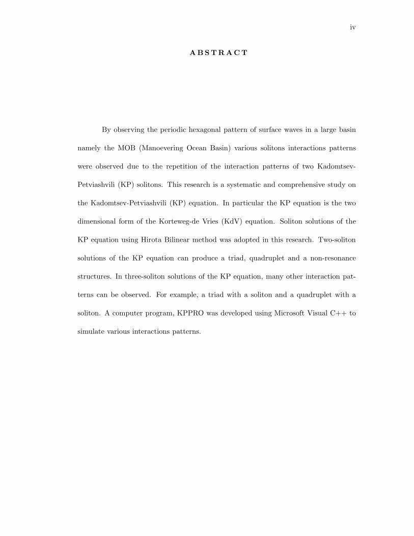
A BS TR ACT
By observing the periodic hexagonal pattern of surface waves in a large basin
namely the MOB (Manoevering Ocean Basin) various solitons interactions patterns
were observed due to the repetition of the interaction patterns of two Kadomtsev-
Petviashvili (KP) solitons. This research is a systematic and comprehensive study on
the Kadomtsev-Petviashvili (KP) equation. In particular the KP equation is the two
dimensional form of the Korteweg-de Vries (KdV) equation. Soliton solutions of the
KP equation using Hirota Bilinear method was adopted in this research. Two-soliton
solutions of the KP equation can produce a triad, quadruplet and a non-resonance
structures. In three-soliton solutions of the KP equation, many other interaction pat-
terns can be observed. For example, a triad with a soliton and a quadruplet with a
soliton. A computer program, KPPRO was developed using Microsoft Visual C++ to
simulate various interactions patterns.
v
A BS TR AK
Dengan memerhatikan bentuk gelombang permukaan dalam sebuah tangki lau-
tan (MOB: “Manoevering Ocean Basin”) berbagai bentuk interaksi soliton telah diper-
hatikan serupa dengan corak ulangan interaksi dua soliton Kadomtsev-Petviashvili
(KP). Penyelidikan ini adalah kajian yang sistematik dan menyeluruh mengenai per-
samaan Kadomtsev-Petviashvili (KP). Secara umumnya, persamaan KP merupakan
sejenis persamaan dua dimensi Korteweg-de Vries (KdV). Penyelesaian persamaan KP
yang menggunakan kaedah Bilinear Hirota dipilih dalam kajian ini. Penyelesaian dua
soliton persamaan KP akan menghasilkan struktur-struktur berbentuk “triad”, kuadru-
plet dan struktur tak beresonan dalam interaksi soliton. Dalam penyelesaian tiga soli-
ton persamaan KP, banyak lagi struktur interaksi soliton dapat diperhatikan. Con-
tohnya antara “triad” dengan satu soliton dan antara kuadruplet dengan satu soliton.
Satu program komputer yang dinamakan sebagai KPPRO telah dibangunkan dengan
menggunakan Microsoft Visual C++ supaya pelbagai struktur interaksi soliton dapat
dihasilkan.

vi
CONTENTS
Declarations ii
Acknowledgements iii
Abstract iv
Abstrak v
Contents vi
List of Figures ix
CHAPTER SUBJECT PAGE
I. INTRODUCTION 1
1.1 Preface 1
1.2 Background of The Problem 2
1.3 Statement of The Problem 2
1.4 Objective of The Study 3
1.5 Importance of The Study 3
1.6 Scope of The Research 4
1.7 Methodology of The Research 4
1.8 History Of Soliton 4
1.8.1 The Korteweg-de Vries (KdV) Equation 6
1.8.2 Properties of Solitons 9
1.8.3 The Kadomtsev-Petviashvili (KP) Equation 13
1.9 Outline Of Report RMC Vot 75023 13
1.10 Conclusion 14
vii
II. INTERACTIONS OF TWO SOLITONS 15
2.1 Introduction 15
2.2 The Kadomtsev-Petviashvili (KP) Equation 15
2.3 Interaction Of Two Solitons 18
2.3.1 Case 1: η1 Fixed; η2 Tends To +∞ 19
2.3.2 Case 2: η1 Fixed; η2 Tends To −∞ 20
2.3.3 Case 3: η2 Fixed; η1 Tends To +∞ 21
2.3.4 Case 4: η2 Fixed; η1 Tends To −∞ 21
2.4 Condition For Resonances 22
2.5 Resonances In The KP Equation 23
2.5.1 Full Resonance: A Triad 23
2.5.2 Partially Resonance: A Quadruplet 24
2.5.3 Non-Resonance: A Cross 25
2.6 Computer Simulation 26
2.7 Conclusion 36
III. INTERACTIONS OF THREE SOLITONS 37
3.1 Introduction 37
3.2 General Solution For Three Solitons 37
3.3 The Wronskian Techniques 40
3.4 Solution For Two Solitons In Full Resonance 41
3.5 Solution For Interaction Between A Triad And A Soliton 43
3.6 Computer Simulation 52
3.6.1 A Triad Interacts With A Soliton 52
3.6.1.1 Type 1: n1 = n2 ≈ n3 52
3.6.1.2 Type 2: n2 = n3 ≈ n1 64
3.6.1.3 Type 3: n1 = n3 ≈ n2 69
viii
3.6.2 A Quadruplet Interacts With A Soliton 74
3.7 Conclusion 79
IV. SUMMARY AND CONCLUSIONS 80
4.1 Introduction 80
4.2 Summary 81
4.3 Suggestion 82
4.4 Application Of The KP Equation 83
4.5 Future Research 85
REFERENCES 87
ix
LIST OF FIGURES
Figure No. Title Page
1.1 Solitary Wave. 8
1.2 3D plot of two-soliton interactions. 11
1.3 Two-soliton interactions at t = −10. 12
1.4 Two-soliton interactions at t = 0 12
1.5 Two-soliton interactions at t = +10. 12
2.1 Contour plot for two-soliton interaction 22
2.2 A triad 24
2.3 A quadruplet 25
2.4 A cross 26
2.5 A triad with n1 = n2 27
2.6 A triad with l1 = l2 28
2.7 Movement of a triad 29
2.8 A quadruplet 30
2.9 The length of resonant soliton with different p 31
2.10 Movement of a quadruplet with p = 10 32
2.11 2D non-resonant soliton 34
2.12 3D non-resonant soliton 34
2.13 Movement of a cross 35
3.1 A triad interacts with a soliton at at t = 0.5s 55
x
3.2 Geometry of a triad interacts with a soliton at t = 0.5s 55
3.3 A triad interacts with a soliton at t = 0s 56
3.4 Geometry of a triad interacts with a soliton at t = 0s 56
3.5 A triad interacts with a soliton at t = −1s 57
3.6 Geometry of a triad interacts with a soliton at t = −1s 57
3.7 Geometry of a triad interacts with a soliton at t = −1s 58
3.8 A triad cross with soliton at t = −1s 61
3.9 A triad cross with soliton at t = 0s 62
3.10 A triad cross with soliton at t = 1s 62
3.11 A triad cross with soliton at t = −1s 63
3.12 A triad cross with soliton at t = 0s 63
3.13 A triad cross with soliton at t = 1s 64
3.14 A triad interacts with soliton at t = 1s 65
3.15 Geometry of a triad interacts with a soliton at t = 1s 66
3.16 A triad interacts with soliton at t = 0.25s 66
3.17 A triad interacts with soliton at t = 0s 67
3.18 A triad interacts with soliton at t = −1s 67
3.19 Geometry of a triad interacts with a soliton at t = −1s 68
3.20 A triad interacts with a soliton at t = 1s 70
3.21 Geometry of a triad interacts with a soliton at t = 1s 70
3.22 A triad interacts with a soliton at t = 0.25s 71
3.23 A triad interacts with a soliton at t = 0s 71
3.24 A triad interacts with a soliton at t = −1s 72
3.25 Geometry of a triad interacts with a soliton at t = −1s 72
3.26 A quadruplet interacts with a soliton at t = 2s 75
3.27 Geometry of a quadruplet interacts with a soliton at t = 2s 75
xi
3.28 A quadruplet interacts with a soliton at t = 0.5s 76
3.29 A quadruplet interacts with a soliton at t = 0s 76
3.30 A quadruplet interacts with a soliton at t = −0.25s 77
3.31 A quadruplet interacts with a soliton at t = −1s 77
3.32 Geometry of a quadruplet interacts with a soliton at t = −1s 78
CHAPTER I
INTRODUCTION
1.1 Preface
More than 170 years ago, the phenomenon of the solitary wave, which was dis-
covered by the famous British scientist, John Scott Russell as early in 1834, has been
greatly concerned with the development of physics and mathematics. Interest in it is
growing constantly-now it has been proved that a large number of the nonlinear evolu-
tion equations have soliton solutions by using numerical calculations and the theoretical
analysis.
Solitary waves have the striking property since they can keep the shape of the
wave unchanged even after interaction. This is similar to the colliding property of
particles. So Kruskal and Zabusky (1965) named them “solitons” due to the recurrence
property. The solitary waves not only have been observed in nature, some of them
recently have also been produced in laboratories.
The theory of soliton is closely related to modern physics. On one hand, this
theory is also applied to explain a lot of physical problems and on the other hand,
the theory of soliton is continuously progressing and developing. We will give a brief
account of the history of soliton theory so as to understand this relationship more
clearly in the literature review section.
1
2
1.2 Background of The Problem
There are many examples of resonance in physics. However, resonance in soli-
ton interaction is an interesting phenomena. In this paper, we will use the Kadomtsev-
Petviashvili (KP) equation to model the two-soliton interactions,Freeman, 1978. In par-
ticular, the KP equation is a two-dimensional of the Korteweg-de Vries (KdV) equation.
Miles (1977),discovered that in the interaction of two solitons, the interaction region
between the incident solitons and the centered-shifted solitons after interaction is essen-
tially itself a single soliton leads to a very simple conceptual picture of the interaction
process. This interaction soliton is the resonant soliton associated with the two incident
solitons.
1.3 Statement of The Problem
A wide range of one-dimensional, nonlinear waves in weakly dispersing media
such as waves in shallow water, ion acoustic and magneto acoustic waves in plasma,
etc. are described by the Korteweg-de Vries equation. This equation can be equally
well applied to media with negative or positive dispersion.
The extension of this equation to motions in more than one dimension were
given by Kadomtsev and Petviashvili (1970), who generalized the dispersion relation
to give an extra term in the equation due to the extra dimension and Satsuma (1976)
had solved the Kadomtsev-Petviashvili (KP) equation by using Bilinear method while
Ong (1993) had studied the solution given by Satsuma.
Earlier studies have indicated that motion of solitons of classical nonlinear evolu-
tion equations for example, the Korteweg-de Vries (KdV) equation and the Kadomtsev-
3
Petviashvili (KP) equation can exhibit resonance. This occurs if certain constraints on
the wave numbers and frequencies of the nonlinear waves are satisfied (Chow, 1997).
Since Satsuma (1976) had solved the KP equation by using Hirota Bilinear method,
therefore it is possible to investigate the interactions patterns for two, three and four
KP solitons resonating among themselves.
1.4 Objective of The Study
The main objectives of this research are to:
1. Study the interactions patterns of two KP solitons.
2. Study the interactions patterns of three KP solitons.
1.5 Importance of The Study
Since we cannot spend so much fund to set up an MOB that is very costly to
maintain, thus this research will provide another avenue to solve KP equation using
KPPRO which is a numerical solver to produce the simulation of interaction patterns
of two and three KP solitons. This research will be at par with the most recent devel-
opments in nonlinear fields especially in the research of soliton. The outcomes of this
research will be published in international journals and talks presented in local and
international colloquiums, conferences and seminars.
4
1.6 Scope of The Research
In this research, we will only consider the positive dispersion of the KP equation
which is shown as below.
(ut + 6uux + uxxx)x − 3uyy = 0. (1.1)
We wish to observe the interactions patterns of two, three and four-soliton
solutions of the above KP equation. Various interactions patterns involving a soliton,
a triad or a quadruplet will be studied.
1.7 Methodology of The Research
This research adopted the analytic solution given by Satsuma (1976) using
Hirota Bilinear method as
u(x, y, t) = 2∂2
∂x2ln f (1.2)
By using this method, we will study the interactions patterns for two, three and four
KP solitons solutions. To solve Equation (1.1), we will develop a computer program
namely KPPRO by using Microsoft Visual C++ Professional Edition to automatically
solve Equation (1.1). Later we will plot the 2D and 3D graphs of soliton interactions.
1.8 History Of Soliton
Solitons made their first appearance in the world of science with the beautiful
report on waves, presented by J. Scott Russell in 1844 at the British Association for the
Advancement of Science. In his ‘Report on Waves’, he vividly wrote (Newell, 1985):
“I believe I shall best introduce the phenomenon by describing the circumstances
5
of my first acquaintance with it. I was observing the motion of a boat which was rapidly
drawn along a narrow channel by a pair of horses, when the boat suddenly stopped-not
so the mass of water in the channel which it had put in motion; it accumulated round
the prow of the vessel in a state of violent agitation, then suddenly leaving it behind,
rolled forward with great velocity, assuming the form of a large solitary elevation, a
rounded, smooth and well-defined heap of water, which continued its course along the
channel apparently without change of form or diminution of speed. I followed it on
horseback, and overtook it still rolling on at a rate of some thirty feet long and a foot
to a foot and half in height. Its height gradually diminished, and after a chase of one or
two miles I lost it in the windings of the channel. Such, in the month of August 1834,
was my first chance interview with that singular and beautiful phenomenon which I
have called the Wave of Translation, a name which it now greatly bears”.
This is the unique phenomenon observed by Russell on the Edinburgh-Glasgow
canal in 1834. Moreover, he thought it to be a stable solution of fluid motion and
coined the word “solitary waves” to name it. However, Russell could not prove his
conclusion or made physicists believe it at that time. Since then, the problems about
solitary waves has caused a wide range of arguments among physicists of the time.
Until 1895, after sixty years, the famous Dutch mathematician Korteweg and
his student de Vries began to study the equation for the motion of the shallow water
waves along a direction using the long wave approximation and the small amplitude
assumption,
∂η
∂t=
32
√g
l
∂
∂x
(12η2 +
23αη +
σ
3∂2η
∂x2
)(1.3)
where η is the height of the peak, l is the depth of the water, g is the gravitational
acceleration, α and σ are physical constants (Guo, 1995). They made complete analysis
on the solitary wave phenomenon and from the above equation, they obtain the pulse
6
like solution of the solitary wave whose shape is not changeable, and is consistent with
Russell’s descriptions about the solitary wave. So the existence of solitary waves was
confirmed by the theory.
In 1965, the famous American physicist and the member of the American Acad-
emy of Science, Kruskal and the physicist Zabusky investigated and analyzed the non-
linear simulation in detail and obtained more complete and rich results, which confirmed
the conclusion that the solitary wave do not change the shapes after the interaction.
Since the solitary waves have the unchangeable property like the collision of particles,
they named them “solitons”.
Kruskal and Zabusky’s work was an important milestone in the history of the
soliton theory. The concept of the “soliton” introduced by them correctly revealed
the substance of solitary waves and had been accepted in general. Hence forward, the
study of soliton theory had been developed more vigorously and caused a world wide
study. Besides the study of solitons in the fields such as fluid dynamics, elementary
particle physics, plasma physics, etc., the solitons were also found one after another
in condensed matter physics, superconductivity physics, laser physics, biophysics etc..
Up to now, a rather complete mathematical and physical theory of soliton has been
formed.
1.8.1 The Korteweg-de Vries (KdV) Equation
Here is a little biography of Korteweg and de Vries. Diederik Johannes Korteweg
(1848-1941) was a student of J. D. van der Waals and received the first doctoral degree
of the University of Amsterdam in 1878 for his dissertation on the motion of a viscous
fluid in an elastic tube, with application to arterial blood flow. He occupied the chair of
7
Mathematics and Mechanics at the same university from 1881 to 1918. His biographical
memoir does not mention any of his work on water waves nor does it cite his 1895 paper
with de Vries.
Korteweg appears to have believe that the paradox posed by the solitary wave,
vis-a-vis the prediction of Airy’s shallow-water theory that long waves in a rectangular
canal must necessarily change their form as they advance, becoming steeper in front and
less steep behind and he suggested the problem of long waves to his student Gustav
de Vries. Biographical data on Gustav de Vries are difficult to obtain (he is not to
be confused with the Dutch mathematician H. de Vries), but it is known that he
was a member of the Wiskundig Genootschap which is Dutch Mathematical Society
from 1892, defended his thesis in 1894 and subsequently taught at the Gymnasiums in
Alkmaar and Haarlem. He had published two papers on cyclones in the Verhandlingen
of the Royal Dutch Academy of Arts and Sciences in 1896 and 1897. The 1895 paper of
Korteweg & de Vries was excerpted and translated from de Vries’s 1894 thesis (Miles,
1981; Kox, 1995; Bullough and Caudrey, 1995).
The equation they used to study long water waves in a rectangular canal was
named after them. The KdV equation is a nonlinear partial differential equation given
by
ut + 6uux + uxxx = 0, (1.4)
where subscripts denote partial differentiations. In general the KdV equation describes
the unidirectional propagation of small but finite amplitude waves in a nonlinear dis-
persive medium.
Historically, Korteweg and de Vries set out to settle the question: If friction is
neglected, do long water waves necessarily continue to steepen in front and become less
8
steep behind? Their answer was no; in particular they showed that Equation (1.4) has
steady progressing wave solutions, namely the solitary wave
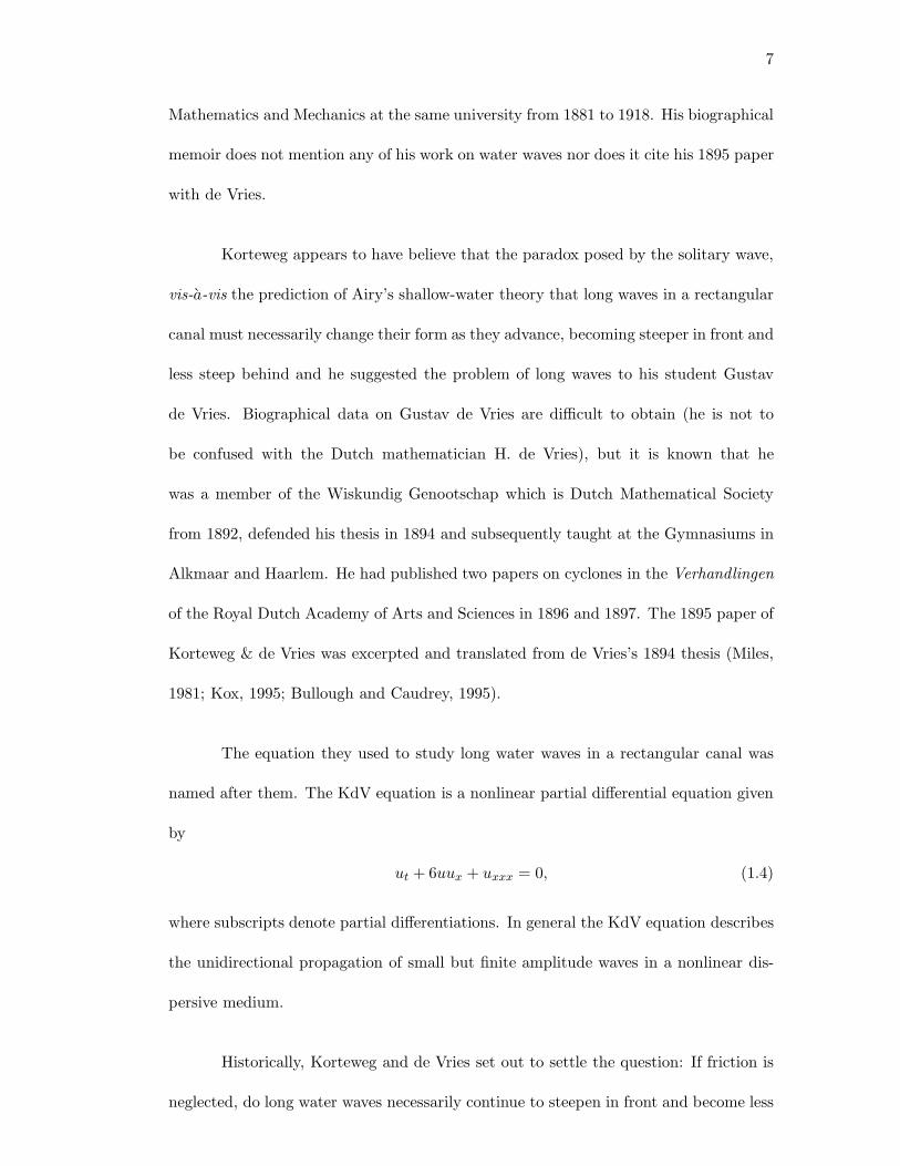
u(x, t) =12a2sech2
[12a
(x − x0 − c2t
)](1.5)
and the periodic cnoidal wave which can be written in terms of Jacobi elliptic functions.
The solitary waves form a one parameter family of pulse-shaped solutions, aside from
the trivial translation in x, where the velocity c2 is proportional to the amplitude,12a2
and the width1a
is inversely proportional to the square root of the amplitude (see
Figure 1.1). Therefore, taller solitary wave travel faster and are narrower than the
shorter ones (Miura, 1978).
Figure 1.1: Solitary Wave
Although many nonlinear dynamical systems have solitary waves associated
with them, the solitary waves of the KdV equation and some other nonlinear evolution
equations has distinguished property. Consider the initial-value problem where two
solitary waves of distinct amplitudes are placed on the real line with the taller one to
9
the left of the shorter one. They should be spaced enough apart so that only their
exponentially small tails overlap (see Figure 1.1).
This initial condition is then evolved in time according to the KdV equation
and because the taller solitary wave is to the left, it will travel faster to the right, catch
up with the shorter one and they will undergo a nonlinear interaction according to the
KdV equation.
Surprisingly, they emerge from the interaction unchanged in waveform and am-
plitude, but slightly shifted from where they would have been had no interaction oc-
curred (see Figure 1.2). It was this particle like properties of the solitary waves which
are:
1. steady progressing pulse like solution, and
2. the preservation of their shape and speeds after interaction
which led Zabusky and Kruskal to call them solitons. Thus a single soliton is a solitary
wave but solitary waves are solitons only if they have the above described properties.
The proof that two solitons emerge from the interaction unchanged was first
given by Lax and the general case of N solitons is obtained using the inverse scattering
method by Gardner, Greene, Kruskal and Miura (1967).
1.8.2 Properties of Solitons
Since the first discovery of solitary waves by Scott Russell, many happenings
about solitary waves were discovered experimentally or theoretically. In 1965, Zabusky
and Kruskal reported the celebrated numerical computation of solutions of the KdV
10
equation and revealed remarkable stability of the solitary waves, each of which behaved
like a “particle”. After an interaction of two solitary waves, each wave restore its
original shape and continues its course of travel. This is an example of the recurrence
process. Thus, the wave behaves like “particle”. Because of this behavior, the solitary
waves are called “solitons”. Solitary waves have the following properties:
1. These localized waves are bell-shaped and travel with permanent form and con-
stant speed.
2. Speed of soliton is proportional to its amplitude, which means, that taller solitary
waves travel faster than shorter ones.
3. The width of a soliton (at half the height) is inversely proportional to the square
root of its amplitude, which mean, that a taller solitary wave is much thinner
compare to the shorter ones.
4. Three fundamental physical quantities namely mass, momentum and energy of
solitons were always conserved. In fact there are infinitely many conserved quan-
tities satisfied by solitons.
5. Solitons can interact with each other without change of shape and will eventually
emerge as it is after the interaction. The only indication that a linear interaction
has not occurred is that the two waves are phase-shifted that is they do not in
the positions after interaction which would be anticipated if each were to move
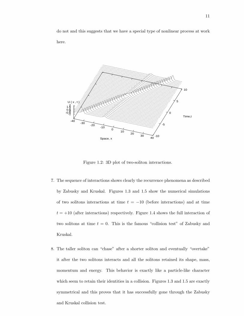
at a constant speed throughout the collision. The 3D plot of this phenomena is
given in Figure 1.2.
6. The taller one, therefore, appears to overtake the shorter one and continue on
its way intact and undistorted. This, of course, is what we would expect if the
two waves were to satisfy the linear superposition principle. But they certainly
11
do not and this suggests that we have a special type of nonlinear process at work
here.
-40-30
-20-10
010
2030
40Space, x-10
-5
0
5
10
Time,t-1-0.50
0.511.52U ( x , t )
Figure 1.2: 3D plot of two-soliton interactions.
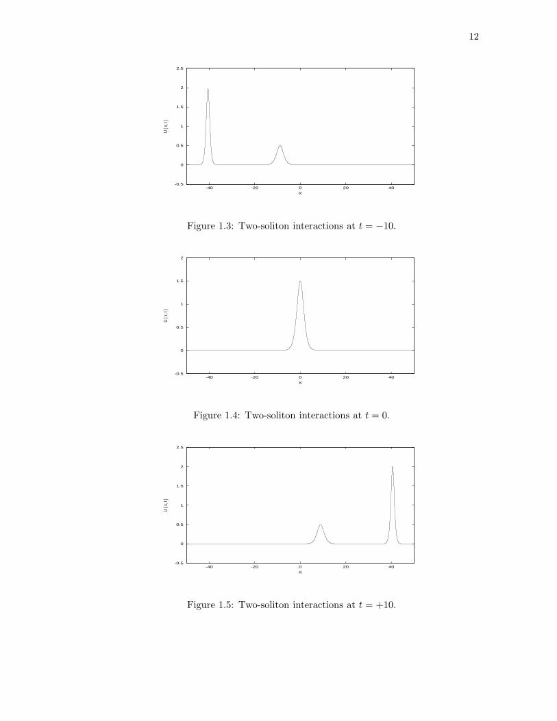
7. The sequence of interactions shows clearly the recurrence phenomena as described
by Zabusky and Kruskal. Figures 1.3 and 1.5 show the numerical simulations
of two solitons interactions at time t = −10 (before interactions) and at time
t = +10 (after interactions) respectively. Figure 1.4 shows the full interaction of
two solitons at time t = 0. This is the famous “collision test” of Zabusky and
Kruskal.
8. The taller soliton can “chase” after a shorter soliton and eventually “overtake”
it after the two solitons interacts and all the solitons retained its shape, mass,
momentum and energy. This behavior is exactly like a particle-like character
which seem to retain their identities in a collision. Figures 1.3 and 1.5 are exactly
symmetrical and this proves that it has successfully gone through the Zabusky
and Kruskal collision test.
12
-0.5
0
0.5
1
1.5
2
2.5
-40 -20 0 20 40
U ( x
, t )
X
Figure 1.3: Two-soliton interactions at t = −10.
-0.5
0
0.5
1
1.5
2
-40 -20 0 20 40
U ( x
, t )
X
Figure 1.4: Two-soliton interactions at t = 0.
-0.5
0
0.5
1
1.5
2
2.5
-40 -20 0 20 40
U ( x
, t )
X
Figure 1.5: Two-soliton interactions at t = +10.
13
1.8.3 The Kadomtsev-Petviashvili (KP) Equation
In the early 1970s, attempts have been made to look for other sort of interactions
apart from one dimensional approximation. Kadomtsev and Petviashvili (1970) used
the idea of the parabolic Leontovich equation and the KdV equation to derive an
equation describing the propagating of weakly non one dimensional acoustic waves in a
dispersive medium. That equation has the same degree of universal applicability as the
KdV equation. Thus, Kadomtsev and Petviashvili proposed a generalization of KdV
equation to two space dimensions. In the differential form the KP equation looks
like
∂
∂x
(∂u
∂t+ 6u
∂u
∂x+
∂3u
∂x3
)+ 3σ2uyy = 0, (1.6)
where u(x, y, t) is a scalar functions and σ2 = ±1. We can simply write the KP equation
as
(ut + 6uux + uxxx)x ± 3uyy = 0, (1.7)
where subscripts denote the derivatives of the corresponding variables. The upper plus
sign in Equation (1.7) pertains to a medium with negative dispersion and the lower
minus sign to positive dispersion (Tajiri and Murakami, 1989).
1.9 Outline Of Report RMC Vot 75023
This report examines the interactions patterns produced by the KP equation.
We will use the analytic solution given by Satsuma (1976) by using Hirota Bilinear
method. Our main interest is the interactions patterns produced by solitons interaction
in the KP equation.
Chapter 2 will discuss about the interactions of two KP solitons. In this chap-
14
ter we will look for the general solution of two KP soliton. After that, we will build a
computer program to generate the wave structure so that we can produce interaction
patterns. Besides that, we also discuss about the condition for resonance to happen and
provide condition for three types of resonances which are full resonance, partially reso-
nance and non resonance to happen. Each of these resonances will produce structures
like triad, quadruplet and a cross. Since we have these resonance structures, we
can discuss more about the interactions of three KP soliton in Chapter 3 that involves
three KP soliton interactions. We will discuss about two types of interactions which are
interactions between triad and a soliton and also interactions between quadruplet and
a soliton. Moreover, in the interactions of triad and a soliton, we have three versions of
interactions where we use the same parametric values but with different sequences. To
have interactions between quadruplet and a soliton, we need to have general solution
for three KP solitons. Hence we show this process of derivation in this chapter. On the
other hand, we also show that the solution for some specific case can be transformed
into Wronskian determinant. The conclusion and summary about our discussion
can be found in the last chapter and we also propose some other research area that we
can do in future.
1.10 Conclusion
This chapter gives an overview of what is going to be discussed in the following
chapters. A good reason on why we do this study is stated in the background of the
problem as well as in the problem statement. The objective of the study was also given
in details. However, there is some limitation in this study and is stated in the scope of
the study. How we carry out the study is mentioned in the methodology of the study
and the outlines of the report is given at the end of this chapter.
CHAPTER II
INTERACTIONS OF TWO SOLITONS
2.1 Introduction
This chapter will discuss about the Kadomtsev-Petviashvili (KP) equation and
the derivation of the general solution for the two KP solitons. Moreover we will look
at the soliton interaction patterns. All illustrations of the interaction patterns were
included in the computer simulation section. Besides that, we will also discuss more
about the condition for resonances to occur.
2.2 The Kadomtsev-Petviashvili (KP) Equation
An extension of the Korteweg-de Vries (KdV) equation to the two-dimensional
case was given by Kadomtsev and Petviashvili in order to discuss the stability of the
one dimensional soliton in weakly dispersive media. It is now called the Kadomtsev-
Petviashvili (KP) equation. This equation describes a slow variations in y direc-
tion of the waves propagating along the x direction. The KP equation is the most
studied of nonlinear integrable equations in three independent variables x, y and t
(Konopelchenko, 1993).
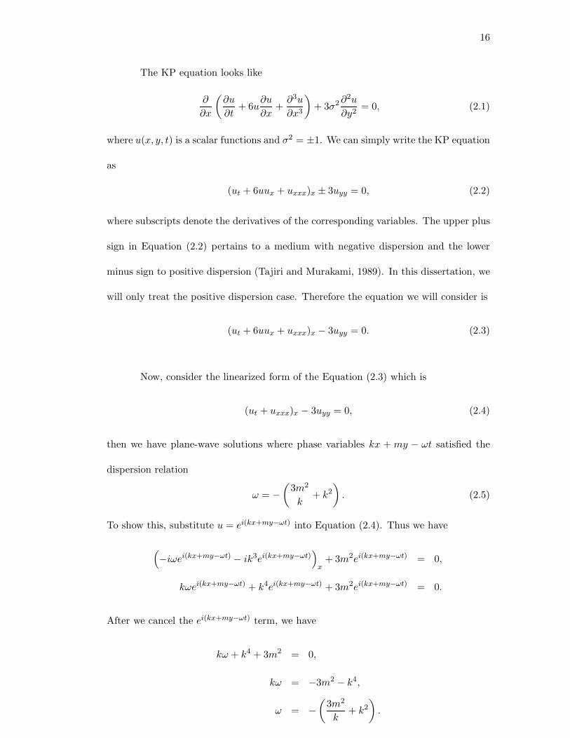
16
The KP equation looks like
∂
∂x
(∂u
∂t+ 6u
∂u
∂x+
∂3u
∂x3
)+ 3σ2 ∂2u
∂y2= 0, (2.1)
where u(x, y, t) is a scalar functions and σ2 = ±1. We can simply write the KP equation
as
(ut + 6uux + uxxx)x ± 3uyy = 0, (2.2)
where subscripts denote the derivatives of the corresponding variables. The upper plus
sign in Equation (2.2) pertains to a medium with negative dispersion and the lower
minus sign to positive dispersion (Tajiri and Murakami, 1989). In this dissertation, we
will only treat the positive dispersion case. Therefore the equation we will consider is
(ut + 6uux + uxxx)x − 3uyy = 0. (2.3)
Now, consider the linearized form of the Equation (2.3) which is
(ut + uxxx)x − 3uyy = 0, (2.4)
then we have plane-wave solutions where phase variables kx + my − ωt satisfied the
dispersion relation
ω = −(
3m2
k+ k2
). (2.5)
To show this, substitute u = ei(kx+my−ωt) into Equation (2.4). Thus we have
(−iωei(kx+my−ωt) − ik3ei(kx+my−ωt)
)x
+ 3m2ei(kx+my−ωt) = 0,
kωei(kx+my−ωt) + k4ei(kx+my−ωt) + 3m2ei(kx+my−ωt) = 0.
After we cancel the ei(kx+my−ωt) term, we have
kω + k4 + 3m2 = 0,
kω = −3m2 − k4,
ω = −(
3m2
k+ k2
).
17
A more convenient way to parameterize this relation is to write k = l+n and m = n2−l2
whence
ω = −(
3(n2 − l2)2
l + n+ (l + n)2
),
= −4(l3 + n3). (2.6)
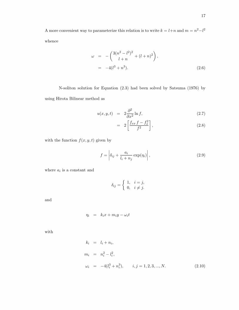
N-soliton solution for Equation (2.3) had been solved by Satsuma (1976) by
using Hirota Bilinear method as
u(x, y, t) = 2∂2
∂x2ln f, (2.7)
= 2[fxx f − f2
x
f2
], (2.8)
with the function f(x, y, t) given by
f =∣∣∣∣δij +
ai
li + njexp(ηi)
∣∣∣∣ , (2.9)
where ai is a constant and
δij ={
1, i = j,0, i 6= j.
and
ηi = kix + miy − ωit
with
ki = li + ni,
mi = n2i − l2i ,
ωi = −4(l3i + n3i ), i, j = 1, 2, 3, ..., N. (2.10)
18
In this chapter we only consider N = 2, therefore we have
f =
∣∣∣∣∣∣∣∣∣∣
1 +a1
l1 + n1exp(η1)
a1
l1 + n2exp(η1)
a2
l2 + n1exp(η2) 1 +
a2
l2 + n2exp(η2)
∣∣∣∣∣∣∣∣∣∣
, (2.11)
f = 1 +a1
l1 + n1exp(η1) +
a2
l2 + n2exp(η2) +
a1
l1 + n1
a2
l2 + n2exp(η1 + η2)
− a1
l1 + n2
a2
l2 + n1exp(η1 + η2),
f = 1 +a1
l1 + n1exp(η1) +
a2
l2 + n2exp(η2)
+ a1a2
((l1 + n2)(l2 + n1) − (l1 + n1)(l2 + n2)(l1 + n2)(l2 + n1)(l1 + n1)(l2 + n2)
)exp(η1 + η2),
f = 1 +a1
l1 + n1exp(η1) +
a2
l2 + n2exp(η2)
+ a1a2
((l1 − l2)(n1 − n1)
(l1 + n2)(l2 + n1)(l1 + n1)(l2 + n2)
)exp(η1 + η2).
Suppose that εi =ai
li + ni, then
f = 1 + ε1 exp(η1) + ε2 exp(η2) +(
(l1 − l2)(n1 − n2)(l1 + n2)(l2 + n1)
)ε1ε2 exp(η1 + η2). (2.12)
Thus we have
f = 1 + ε1 exp(η1) + ε2 exp(η2) + A12ε1ε2 exp(η1 + η2), (2.13)
where
A12 =(l1 − l2)(n1 − n2)(l1 + n2)(l2 + n1)
. (2.14)
2.3 Interaction Of Two Solitons
We will use the function f(x, y, t) which is given in Equation (2.13) to study the
position of each soliton while interacting. Hence we have the following 4 cases (Ong,
1993).
19
2.3.1 Case 1: η1 Fixed; η2 Tends To +∞
In this case, we can observe that the value of 1+ε1 exp(η1) is very small compared
to the value of ε2 exp(η2)+A12ε1ε2 exp(η1+η2). Therefore Equation (2.13) will produce
f ≈ ε2 exp(η2) + A12ε1ε2 exp(η1 + η2),
≈ ε2 exp(η2) [1 + A12ε1 exp(η1)] . (2.15)
We know that η2 is a linear function of x, therefore it will become zero after we
differentiate it twice with respect to x. To explain this, let say we take
f = exp(η)(Q(x)). (2.16)
Substitute the above equation into Equation (2.7), then we have
u = 2∂2
∂x2ln(exp(η)Q(x)),
= 2∂2
∂x2(ln exp(η) + lnQ(x)),
= 2∂2
∂x2(η) + 2
∂2
∂x2(ln Q(x)),
= 0 + 2∂2
∂x2(lnQ(x)).
From the above result, it is shown that we can cancel the exp(η) term without affecting
the value of u. Thus we can use the same concept on Equation (2.15).
u = 2∂2
∂x2ln(ε2 exp(η2) [1 + A12ε1 exp(η1)]),
= 2∂2
∂x2(ln ε2 + ln exp(η2) + ln [1 + A12ε1 exp(η1)]),
= 2∂2
∂x2(ln ε2) + 2
∂2
∂x2(η2) + 2
∂2
∂x2(ln [1 + A12ε1 exp(η1)]),
= 0 + 0 + 2∂2
∂x2(ln [1 + A12ε1 exp(η1)]).
20
Hence our function f(x, y, t) will becomes
f ≈ 1 + A12ε1 exp(η1),
≈ 1 + ε1 exp(η1 + lnA12). (2.17)
From Equation (2.15) and Equation (2.17), we noticed that they are different
equation but still produced same soliton. We named the soliton by Equation (2.17) as
soliton 1* and denoted by S∗1 . This soliton is centered at
η1 + lnA12 = 0. (2.18)
There is a phase shift of lnA12.
2.3.2 Case 2: η1 Fixed; η2 Tends To −∞
Since exp(η2) and A12ε1ε2 exp(η1 + η2) tends to zero, thus the function f(x, y, t)
in Equation (2.13) becomes
f ≈ 1 + ε1 exp(η1) (2.19)
Soliton solution produced by Equation (2.19) has the same characteristic with
soliton by Equation (2.17). The only difference is their position. Thus, we named the
soliton produced by Equation (2.19) as soliton 1 and denoted by S1. This soliton has
center at η1 = 0 and we also noticed that there is no phase shift of lnA12.
21
2.3.3 Case 3: η2 Fixed; η1 Tends To +∞
With the above condition, the function f(x, y, t) in Equation (2.13) becomes
f ≈ ε1 exp(η1) + A12ε1ε2 exp(η1 + η2) (2.20)
because the value of ε1 exp(η1) and A12ε1ε2 exp(η1+η2) are larger that 1 and ε2 exp(η2).
Thus from Equation (2.20)
f = ε1 exp(η1) [1 + A12ε2 exp(η2)] . (2.21)
By using the same concept when deriving Equation (2.17), we obtained
f = 1 + A12ε2 exp(η2),
= 1 + ε2 exp(η2 + lnA12). (2.22)
We called this soliton as soliton 2*, denoted by S∗2 and centered at
η2 + lnA12 = 0. In this case there is a phase shift of lnA12.
2.3.4 Case 4: η2 Fixed; η1 Tends To −∞
In this case, we found that the value ε1 exp(η1) and A12ε1ε2 exp(η1 + η2) become
very small compared to 1 and ε1 exp(η2) and thus Equation (2.13) becomes
f ≈ 1 + ε2 exp(η2). (2.23)
The soliton given by Equation (2.23) is named as soliton 2 and denoted by S2. This
soliton is centered at η2 = 0 and there is no phase shift.
22
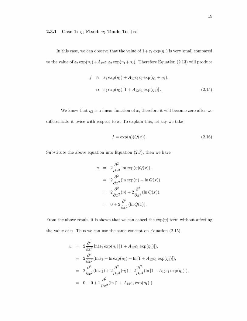
By using the result from the above 4 cases, we have an illustration as given in
Figure 2.1.
S1 : η1 = 0
S2 : η2 = 0
S12
S∗1 : η1 + lnA12 = 0
S∗2 : η2 + lnA12 = 0
.............................................
............................................
.............................................
.............................................
.............................................
.............................................
..........................................
.............................................................................................................................................................................................................................................................................................................
................................
................................
................................
................................
................................
................................
................................
................................
................................
.
.............................................................................................................................................................................................................................................................................................................
.................................................................................................................................................................................................................................................................................................
Figure 2.1: Contour plot for two-soliton interaction
2.4 Condition For Resonances
From Figure 2.1, it can be observed that the length of S12 depends on lnA12.
The bigger the value of lnA12, the longer S12 will be. Therefore we can conclude that
resonance will only occurs when
lnA12 → −∞, (2.24)
or
A12 → 0, (2.25)
In this dissertation, we will only consider A12 tends to zero as a condition for resonance.

23
2.5 Resonances In The KP Equation
Miles (1977b) in his study discovered that when two solitons interact, they will
form one soliton only which is shown in Figure 2.1 (Anker and Freeman, 1978). This
phenomenon is called resonance. There are three types of resonances in the KP solitons
interaction which are full resonance, partial resonance and non-resonance. Resonance
will only occurs when the value of A12 is approaching zero. Therefore the values of
n1, n2, l1 and l2 will determined the resonant structure. If we fix the values of l1 and
l2, then n1 and n2 will determined the value of A12.
2.5.1 Full Resonance: A Triad
As mentioned above, we should fix the value of A12 close to zero in order for
resonance to occur. From Equation (2.14), it can be observed that we have to fix the
value of n1 = n2 or l1 = l2 in order to make the value of A12 to be close to zero. If we
fix the value of l1 and l2 with real number but l1 6= l2, then the resonances occurrence
will be determined by the value of n1 and n2 or the other way round. For the full
resonance case, as A12 = 0 (n1 = n2), Equation (2.13) will become
f = 1︸︷︷︸(1)
+ ε1 exp(η1)︸ ︷︷ ︸(2)
+ ε2 exp(η2)︸ ︷︷ ︸(3)
. (2.26)
Any combination of (1), (2) and (3) from Equation (2.26) will form another
soliton which is the first soliton, S1, the second soliton, S2 and the resonant soliton,
S12 and they can be represented by the combination of (12), (13) and (23) respectively.
Soliton S1, (12) : f = 1 + ε1 exp(η1), (2.27)
Soliton S2, (13) : f = 1 + ε2 exp(η2), (2.28)
Soliton S12, (23) : f = ε1 exp(η1) + ε2 exp(η2). (2.29)
24
By referring to Figure 2.1, when the value of A12 tends to zero, lnA12 will
approach infinity. Thus the length of the resonant soliton will tends to be very long
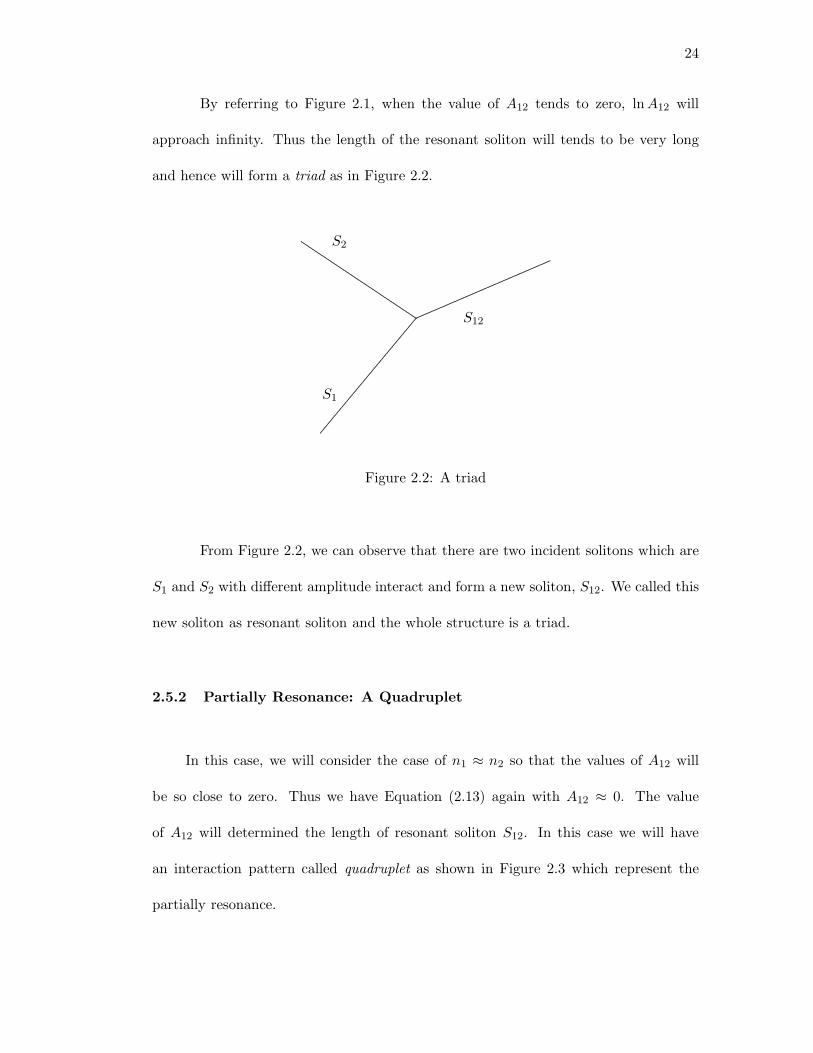
and hence will form a triad as in Figure 2.2.
S1
S2
S12....................
........................................
........................................
........................................
........................................
........................................
........................................
................
...........................................................................................................................................................................................................................................................................................
............................
............................
.............................
............................
............................
.............................
............................
............................
.............................
......
Figure 2.2: A triad
From Figure 2.2, we can observe that there are two incident solitons which are
S1 and S2 with different amplitude interact and form a new soliton, S12. We called this
new soliton as resonant soliton and the whole structure is a triad.
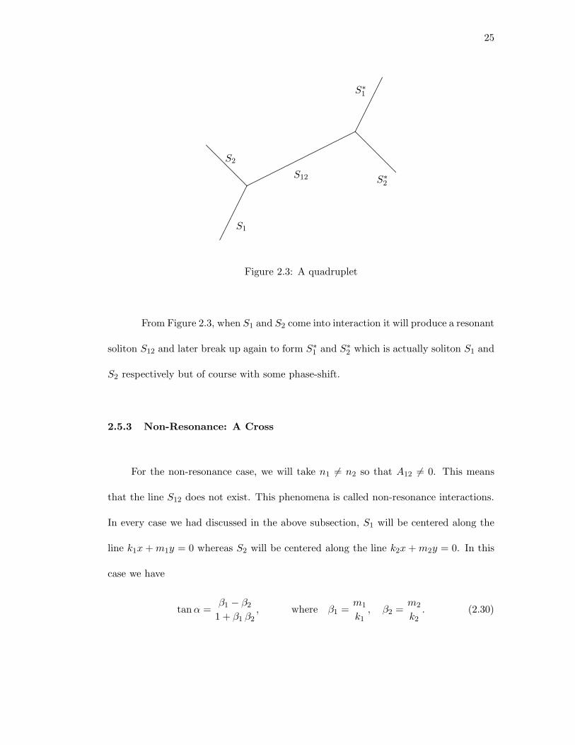
2.5.2 Partially Resonance: A Quadruplet
In this case, we will consider the case of n1 ≈ n2 so that the values of A12 will
be so close to zero. Thus we have Equation (2.13) again with A12 ≈ 0. The value
of A12 will determined the length of resonant soliton S12. In this case we will have
an interaction pattern called quadruplet as shown in Figure 2.3 which represent the
partially resonance.
25
S1
S2
S12
S∗1
S∗2.................
....................................
...................................
...................................
...................................
...................................
...................................
...................................
...................................
..........................
..................................................................................................................................................................
.......................
......................
.......................
.......................
......................
.......................
..................
..........................................................................................................................................................
..................................................................................................................................................................
Figure 2.3: A quadruplet
From Figure 2.3, when S1 and S2 come into interaction it will produce a resonant
soliton S12 and later break up again to form S∗1 and S∗
2 which is actually soliton S1 and
S2 respectively but of course with some phase-shift.
2.5.3 Non-Resonance: A Cross
For the non-resonance case, we will take n1 6= n2 so that A12 6= 0. This means
that the line S12 does not exist. This phenomena is called non-resonance interactions.
In every case we had discussed in the above subsection, S1 will be centered along the
line k1x + m1y = 0 whereas S2 will be centered along the line k2x + m2y = 0. In this
case we have
tan α =β1 − β2
1 + β1 β2, where β1 =
m1
k1, β2 =
m2
k2. (2.30)
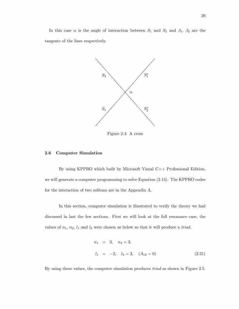
26
In this case α is the angle of interaction between S1 and S2 and β1, β2 are the
tangents of the lines respectively.
S1
S2 S∗1
S∗2
α
..................................................................................................................................................................................................................................................................................................................................................................................................................................................................................................................................................................................................................................................................................................................................................................................................................................................................................................................................................................................................................................................................................................................................................................................................
Figure 2.4: A cross
2.6 Computer Simulation
By using KPPRO which built by Microsoft Visual C++ Professional Edition,
we will generate a computer programming to solve Equation (2.13). The KPPRO codes
for the interaction of two solitons are in the Appendix A.
In this section, computer simulation is illustrated to verify the theory we had
discussed in last the few sections. First we will look at the full resonance case, the
values of n1, n2, l1 and l2 were chosen as below so that it will produce a triad.
n1 = 3, n2 = 3,
l1 = −2, l2 = 3, (A12 = 0) (2.31)
By using these values, the computer simulation produces triad as shown in Figure 2.5.
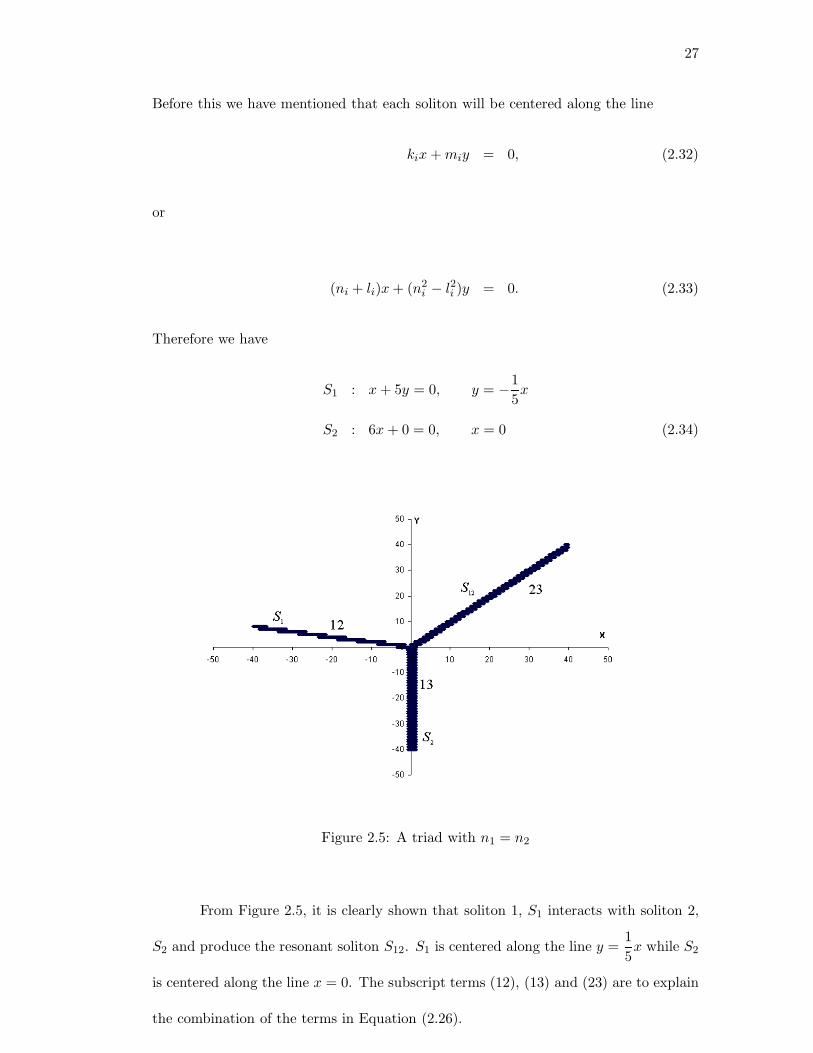
27
Before this we have mentioned that each soliton will be centered along the line
kix + miy = 0, (2.32)
or
(ni + li)x + (n2i − l2i )y = 0. (2.33)
Therefore we have
S1 : x + 5y = 0, y = −15x
S2 : 6x + 0 = 0, x = 0 (2.34)
Figure 2.5: A triad with n1 = n2
From Figure 2.5, it is clearly shown that soliton 1, S1 interacts with soliton 2,
S2 and produce the resonant soliton S12. S1 is centered along the line y =15x while S2
is centered along the line x = 0. The subscript terms (12), (13) and (23) are to explain
the combination of the terms in Equation (2.26).
28
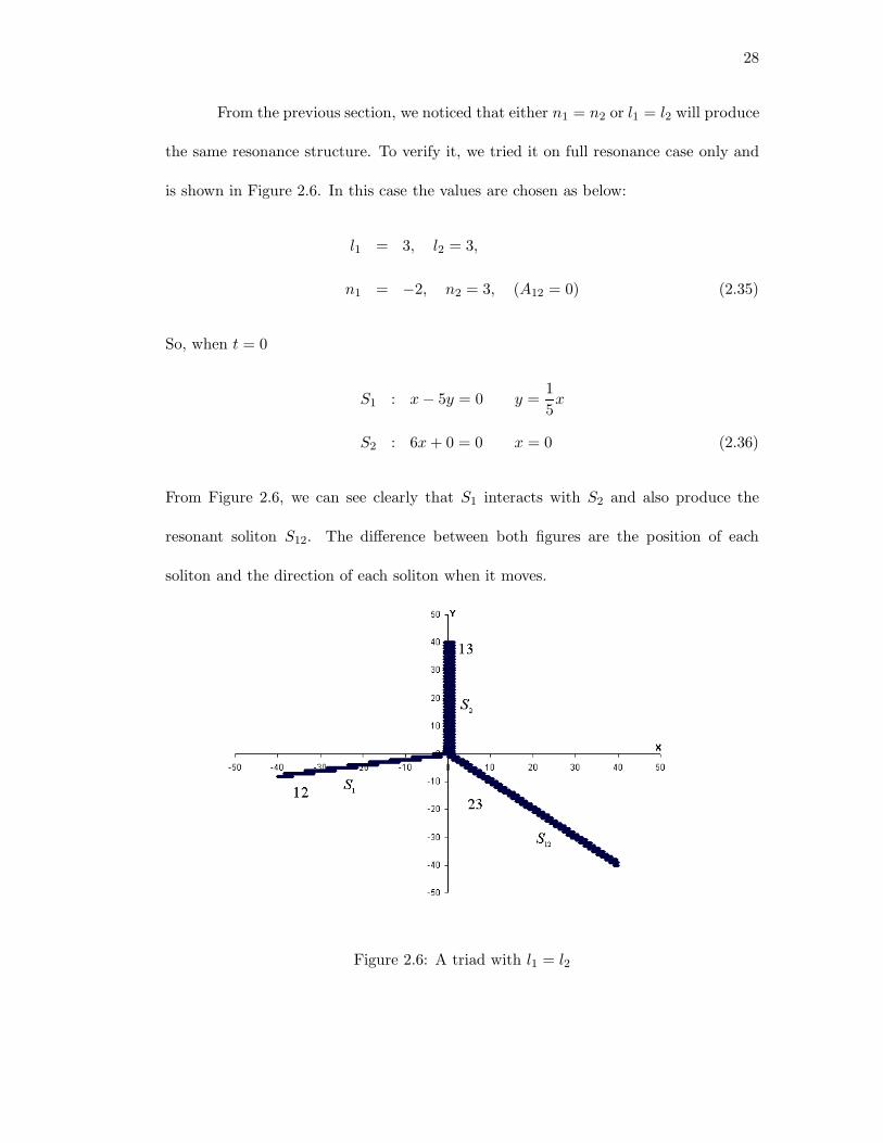
From the previous section, we noticed that either n1 = n2 or l1 = l2 will produce
the same resonance structure. To verify it, we tried it on full resonance case only and
is shown in Figure 2.6. In this case the values are chosen as below:
l1 = 3, l2 = 3,
n1 = −2, n2 = 3, (A12 = 0) (2.35)
So, when t = 0
S1 : x − 5y = 0 y =15x
S2 : 6x + 0 = 0 x = 0 (2.36)
From Figure 2.6, we can see clearly that S1 interacts with S2 and also produce the
resonant soliton S12. The difference between both figures are the position of each
soliton and the direction of each soliton when it moves.
Figure 2.6: A triad with l1 = l2
29
Figure 2.7a: t = −0.25
Figure 2.7b: t = 0
Figure 2.7c: t = −0.25
Figure 2.7: Movement of a triad
30
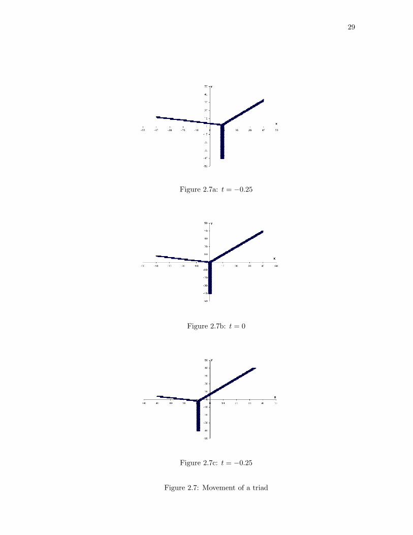
A triad will move as one entity as t changes. This is shown in Figure 2.7. The
only difference is the phase shift. We can notice that Figure 2.7a is symmetry with
Figure 2.7c.
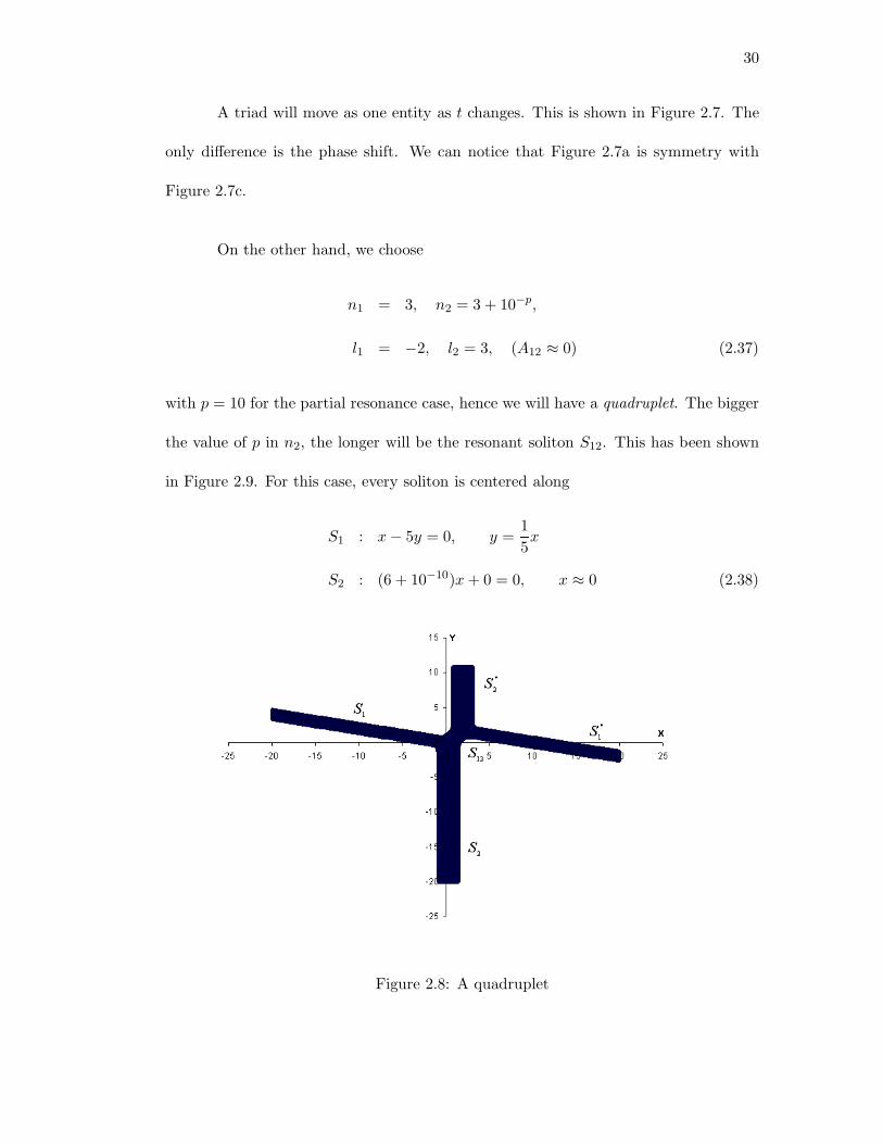
On the other hand, we choose
n1 = 3, n2 = 3 + 10−p,
l1 = −2, l2 = 3, (A12 ≈ 0) (2.37)
with p = 10 for the partial resonance case, hence we will have a quadruplet. The bigger
the value of p in n2, the longer will be the resonant soliton S12. This has been shown
in Figure 2.9. For this case, every soliton is centered along
S1 : x − 5y = 0, y =15x
S2 : (6 + 10−10)x + 0 = 0, x ≈ 0 (2.38)
Figure 2.8: A quadruplet
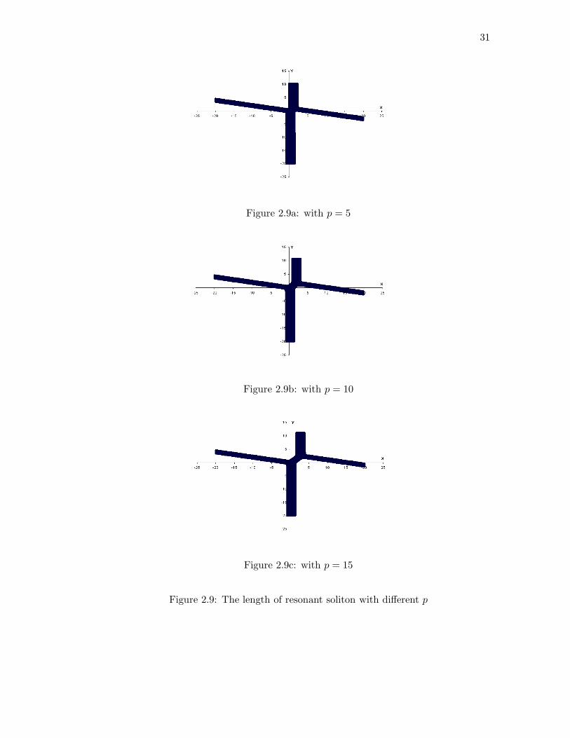
31
Figure 2.9a: with p = 5
Figure 2.9b: with p = 10
Figure 2.9c: with p = 15
Figure 2.9: The length of resonant soliton with different p
32
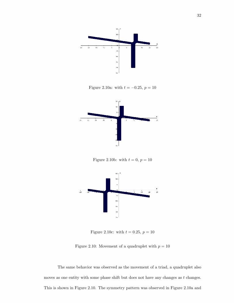
Figure 2.10a: with t = −0.25, p = 10
Figure 2.10b: with t = 0, p = 10
Figure 2.10c: with t = 0.25, p = 10
Figure 2.10: Movement of a quadruplet with p = 10
The same behavior was observed as the movement of a triad, a quadruplet also
moves as one entity with some phase shift but does not have any changes as t changes.
This is shown in Figure 2.10. The symmetry pattern was observed in Figure 2.10a and
33
Figure 2.10c
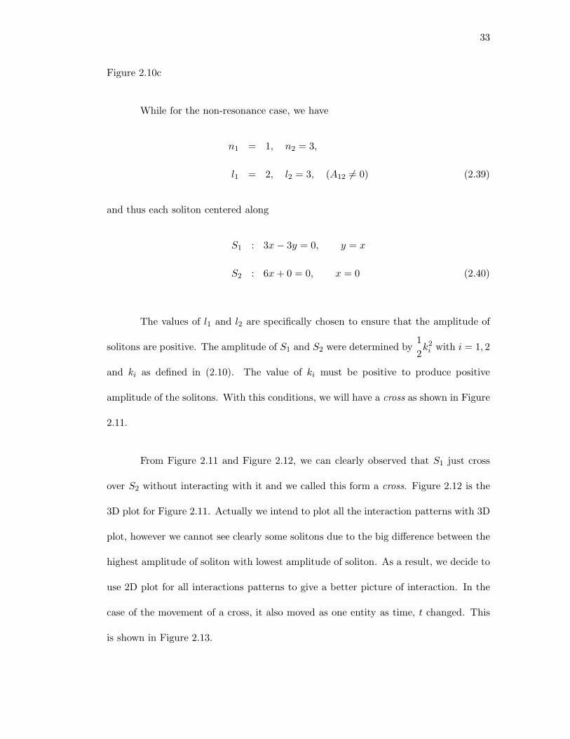
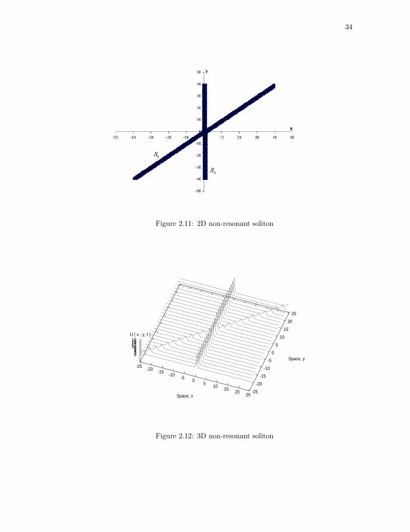
While for the non-resonance case, we have
n1 = 1, n2 = 3,
l1 = 2, l2 = 3, (A12 6= 0) (2.39)
and thus each soliton centered along
S1 : 3x − 3y = 0, y = x
S2 : 6x + 0 = 0, x = 0 (2.40)
The values of l1 and l2 are specifically chosen to ensure that the amplitude of
solitons are positive. The amplitude of S1 and S2 were determined by12k2
i with i = 1, 2
and ki as defined in (2.10). The value of ki must be positive to produce positive
amplitude of the solitons. With this conditions, we will have a cross as shown in Figure
2.11.
From Figure 2.11 and Figure 2.12, we can clearly observed that S1 just cross
over S2 without interacting with it and we called this form a cross. Figure 2.12 is the
3D plot for Figure 2.11. Actually we intend to plot all the interaction patterns with 3D
plot, however we cannot see clearly some solitons due to the big difference between the
highest amplitude of soliton with lowest amplitude of soliton. As a result, we decide to
use 2D plot for all interactions patterns to give a better picture of interaction. In the
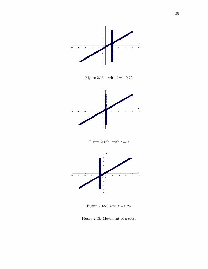
case of the movement of a cross, it also moved as one entity as time, t changed. This
is shown in Figure 2.13.
34
Figure 2.11: 2D non-resonant soliton
-25-20
-15-10
-50
510
1520
25Space, x-25
-20
-15
-10
-5
0
5
10
15
20
25
Space, y024681012141618
U ( x , y, t )
Figure 2.12: 3D non-resonant soliton
35
Figure 2.13a: with t = −0.25
Figure 2.13b: with t = 0
Figure 2.13c: with t = 0.25
Figure 2.13: Movement of a cross
36
2.7 Conclusion
In this chapter, we have shown that resonance in two KP soliton interactions
will form interaction patterns which are triad, quadruplet and cross. These basic pat-
terns will lead us to see more about resonances in KP N-soliton interactions such as
three-soliton interactions and four-soliton interactions in the following chapter. All the
movement of triad, quadruplet and cross move as an entity. This is again another
evidence that these structures are indeed soliton in nature.
CHAPTER III
INTERACTIONS OF THREE SOLITONS
3.1 Introduction
In this chapter, we will discuss more about three KP solitons’ interactions. First
we will look at the derivation of general solution for three KP solitons’ interactions.
Then we can observe the interactions between a triad with a soliton and the interaction
between a quadruplet and a soliton. Besides that, we also can show that the solution
of interactions between triad and a soliton is Wronskian determinant.
Then, we showed that in some cases we can simplify the process of searching
the function f(x, y, t). We will also look at the illustration of the interaction of three
solitons. Computer simulation provides clear evidences and able to verify it accurately.
3.2 General Solution For Three Solitons
In this section, the derivation of the general soliton solution for three-soliton
interactions are shown. The KP equation that we consider is
(ut + 6uux + uxxx)x − 3uyy = 0. (3.1)
This equation had been solved by Satsuma (1976) by using Hirota Bilinear method as
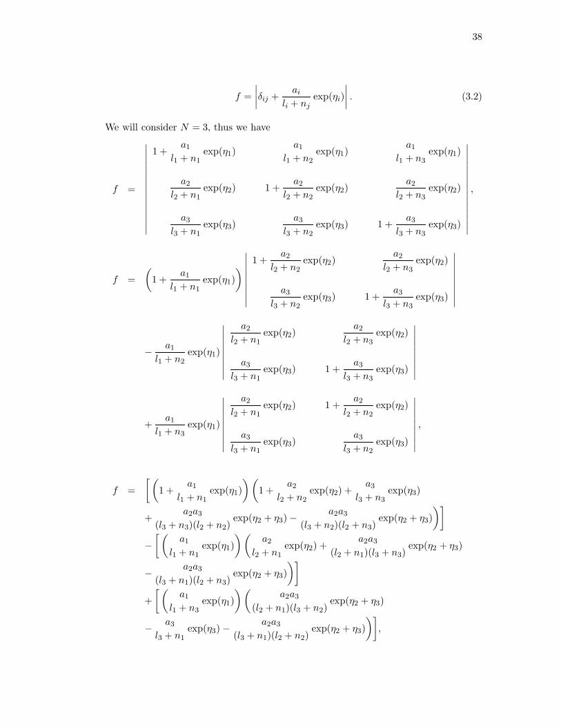
38
f =∣∣∣∣δij +
ai
li + njexp(ηi)
∣∣∣∣ . (3.2)
We will consider N = 3, thus we have
f =
∣∣∣∣∣∣∣∣∣∣∣∣∣∣∣
1 +a1
l1 + n1exp(η1)
a1
l1 + n2exp(η1)
a1
l1 + n3exp(η1)
a2
l2 + n1exp(η2) 1 +
a2
l2 + n2exp(η2)
a2
l2 + n3exp(η2)
a3
l3 + n1exp(η3)
a3
l3 + n2exp(η3) 1 +
a3
l3 + n3exp(η3)
∣∣∣∣∣∣∣∣∣∣∣∣∣∣∣
,
f =(
1 +a1
l1 + n1exp(η1)
)∣∣∣∣∣∣∣∣∣
1 +a2
l2 + n2exp(η2)
a2
l2 + n3exp(η2)
a3
l3 + n2exp(η3) 1 +
a3
l3 + n3exp(η3)
∣∣∣∣∣∣∣∣∣
− a1
l1 + n2exp(η1)
∣∣∣∣∣∣∣∣∣
a2
l2 + n1exp(η2)
a2
l2 + n3exp(η2)
a3
l3 + n1exp(η3) 1 +
a3
l3 + n3exp(η3)
∣∣∣∣∣∣∣∣∣
+a1
l1 + n3exp(η1)
∣∣∣∣∣∣∣∣∣
a2
l2 + n1exp(η2) 1 +
a2
l2 + n2exp(η2)
a3
l3 + n1exp(η3)
a3
l3 + n2exp(η3)
∣∣∣∣∣∣∣∣∣,
f =[(
1 +a1
l1 + n1exp(η1)
)(1 +
a2
l2 + n2exp(η2) +
a3
l3 + n3exp(η3)
+a2a3
(l3 + n3)(l2 + n2)exp(η2 + η3) −
a2a3
(l3 + n2)(l2 + n3)exp(η2 + η3)
)]
−[(
a1
l1 + n1exp(η1)
) (a2
l2 + n1exp(η2) +
a2a3
(l2 + n1)(l3 + n3)exp(η2 + η3)
− a2a3
(l3 + n1)(l2 + n3)exp(η2 + η3)
)]
+[(
a1
l1 + n3exp(η1)
) (a2a3
(l2 + n1)(l3 + n2)exp(η2 + η3)
− a3
l3 + n1exp(η3) −
a2a3
(l3 + n1)(l2 + n2)exp(η2 + η3)
)],
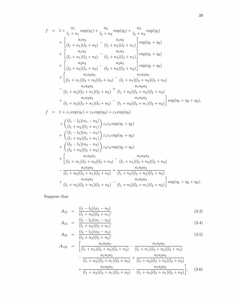
39
f = 1 +a1
l1 + n1exp(η1) +
a2
l2 + n2exp(η2) +
a3
l3 + n3exp(η3)
+[
a1a2
(l1 + n1)(l2 + n2)− a1a2
(l1 + n2)(l2 + n1)
]exp(η1 + η2)
+[
a1a3
(l1 + n1)(l3 + n3)− a1a3
(l1 + n3)(l3 + n1)
]exp(η1 + η3)
+[
a2a3
(l2 + n2)(l3 + n3)− a2a3
(l2 + n3)(l3 + n2)
]exp(η2 + η3)
+[
a1a2a3
(l1 + n1)(l2 + n2)(l3 + n3)− a1a2a3
(l1 + n1)(l3 + n2)(l2 + n3)
− a1a2a3
(l1 + n2)(l2 + n1)(l3 + n3)+
a1a2a3
(l1 + n2)(l3 + n2)(l2 + n3)
+a1a2a3
(l1 + n3)(l2 + n1)(l3 + n2)− a1a2a3
(l1 + n3)(l3 + n1)(l2 + n2)
]exp(η1 + η2 + η3),
f = 1 + ε1 exp(η1) + ε2 exp(η2) + ε3 exp(η3)
+(
(l1 − l2)(n1 − n2)(l1 + n2)(l2 + n1)
)ε1ε2 exp(η1 + η2)
+(
(l1 − l3)(n1 − n3)(l1 + n3)(l3 + n1)
)ε1ε3 exp(η1 + η3)
+(
(l2 − l3)(n2 − n3)(l2 + n3)(l3 + n2)
)ε2ε3 exp(η2 + η3)
+[
a1a2a3
(l1 + n1)(l2 + n2)(l3 + n3)− a1a2a3
(l1 + n1)(l3 + n2)(l2 + n3)
− a1a2a3
(l1 + n2)(l2 + n1)(l3 + n3)+
a1a2a3
(l1 + n2)(l3 + n2)(l2 + n3)
+a1a2a3
(l1 + n3)(l2 + n1)(l3 + n2)− a1a2a3
(l1 + n3)(l3 + n1)(l2 + n2)
]exp(η1 + η2 + η3).
Suppose that
A12 =(l1 − l2)(n1 − n2)(l1 + n2)(l2 + n1)
, (3.3)
A13 =(l1 − l3)(n1 − n3)(l1 + n3)(l3 + n1)
, (3.4)
A23 =(l2 − l3)(n2 − n3)(l2 + n3)(l3 + n2)
, (3.5)
A123 =[
a1a2a3
(l1 + n1)(l2 + n2)(l3 + n3)− a1a2a3
(l1 + n1)(l3 + n2)(l2 + n3)
− a1a2a3
(l1 + n2)(l2 + n1)(l3 + n3)+
a1a2a3
(l1 + n2)(l3 + n2)(l2 + n3)
+a1a2a3
(l1 + n3)(l2 + n1)(l3 + n2)− a1a2a3
(l1 + n3)(l3 + n1)(l2 + n2)
], (3.6)
40
therefore f(x, y, t) becomes
f = 1 + ε1 exp(η1) + ε2 exp(η2) + ε3 exp(η3)
+A12ε1ε2 exp(η1 + η2) + A13ε1ε3 exp(η1 + η3)
+A23ε2ε3 exp(η2 + η3) + A123ε1ε2ε3 exp(η1 + η2 + η3). (3.7)
From this derivations, it can be observed that the derivation of the general
solution for three solitons interactions is complicated. It will be more complicated
as N increases because we are looking for the determinant of a matrix. After the
general solution had been obtained, we can use this solution to produce a sequence of
interactions. For example, we can observe the interaction when a triad interacts with
a soliton, a quadruplet interacts with a soliton and so on. However, for some cases we
can simplify the process of searching the function of f(x, y, t). For example, the process
to get the function f(x, y, t) in the interaction between a triad and a soliton can be
simplify into Wronskian determinant which will be discussed in the following section.
3.3 The Wronskian Techniques
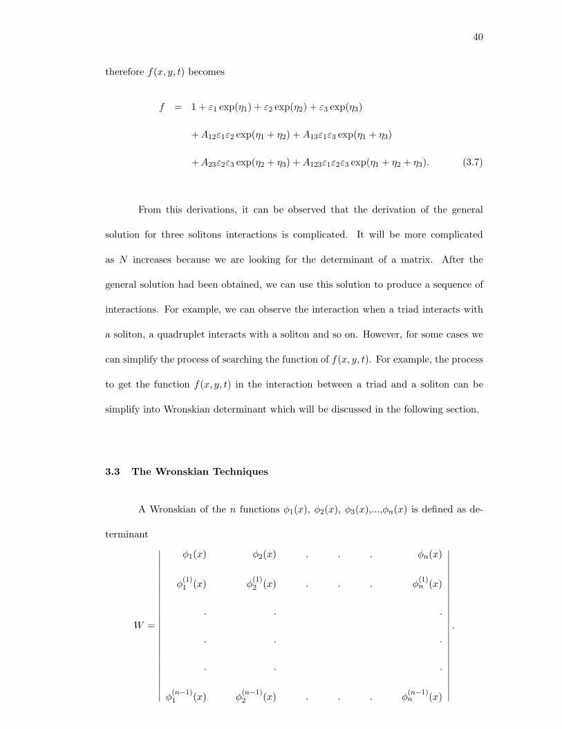
A Wronskian of the n functions φ1(x), φ2(x), φ3(x),...,φn(x) is defined as de-
terminant
W =
∣∣∣∣∣∣∣∣∣∣∣∣∣∣∣∣∣∣∣∣∣∣∣∣∣
φ1(x) φ2(x) . . . φn(x)
φ(1)1 (x) φ
(1)2 (x) . . . φ
(1)n (x)
. . .
. . .
. . .
φ(n−1)1 (x) φ
(n−1)2 (x) . . . φ
(n−1)n (x)
∣∣∣∣∣∣∣∣∣∣∣∣∣∣∣∣∣∣∣∣∣∣∣∣∣
.
41
This is often written as W (φ1(x), φ2(x), ..., φn(x)) (Freeman, 1984; Mukheta,
1989). For our discussion, the KP equation we considered is Equation (3.1). It is well
known that this equation has soliton solutions which can best be expressed in the form
u = 2∂2
∂x2ln f. (3.8)
The N -soliton solution of this equation has been obtained by Satsuma (1976) in Equa-
tion (3.2) and can be written in the form
f =∣∣∣∣δij +
ai
li + njexp(θi + γj)
∣∣∣∣ (3.9)
where
θi = lix − l2i y + 4l3i t, (3.10)
γj = njx + n2jy + 4n3
j t (3.11)
with δij is Kronecker delta, li, ni and ai are real constants and i, j = 1, 2, ..., N . Freeman
and Nimmo (1983) had showed that the above determinant which is Equation (3.2) or
Equation (3.9) is a Wronskian determinant.
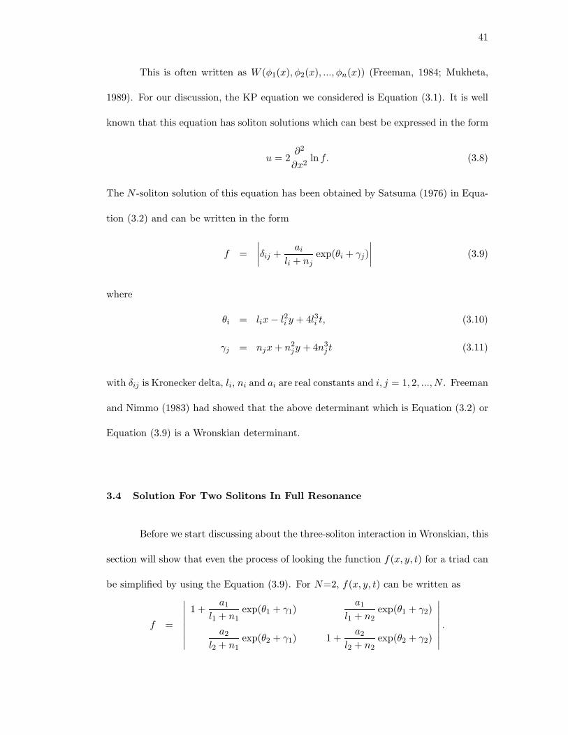
3.4 Solution For Two Solitons In Full Resonance
Before we start discussing about the three-soliton interaction in Wronskian, this
section will show that even the process of looking the function f(x, y, t) for a triad can
be simplified by using the Equation (3.9). For N=2, f(x, y, t) can be written as
f =
∣∣∣∣∣∣∣∣
1 +a1
l1 + n1exp(θ1 + γ1)
a1
l1 + n2exp(θ1 + γ2)
a2
l2 + n1exp(θ2 + γ1) 1 +
a2
l2 + n2exp(θ2 + γ2)
∣∣∣∣∣∣∣∣.
42
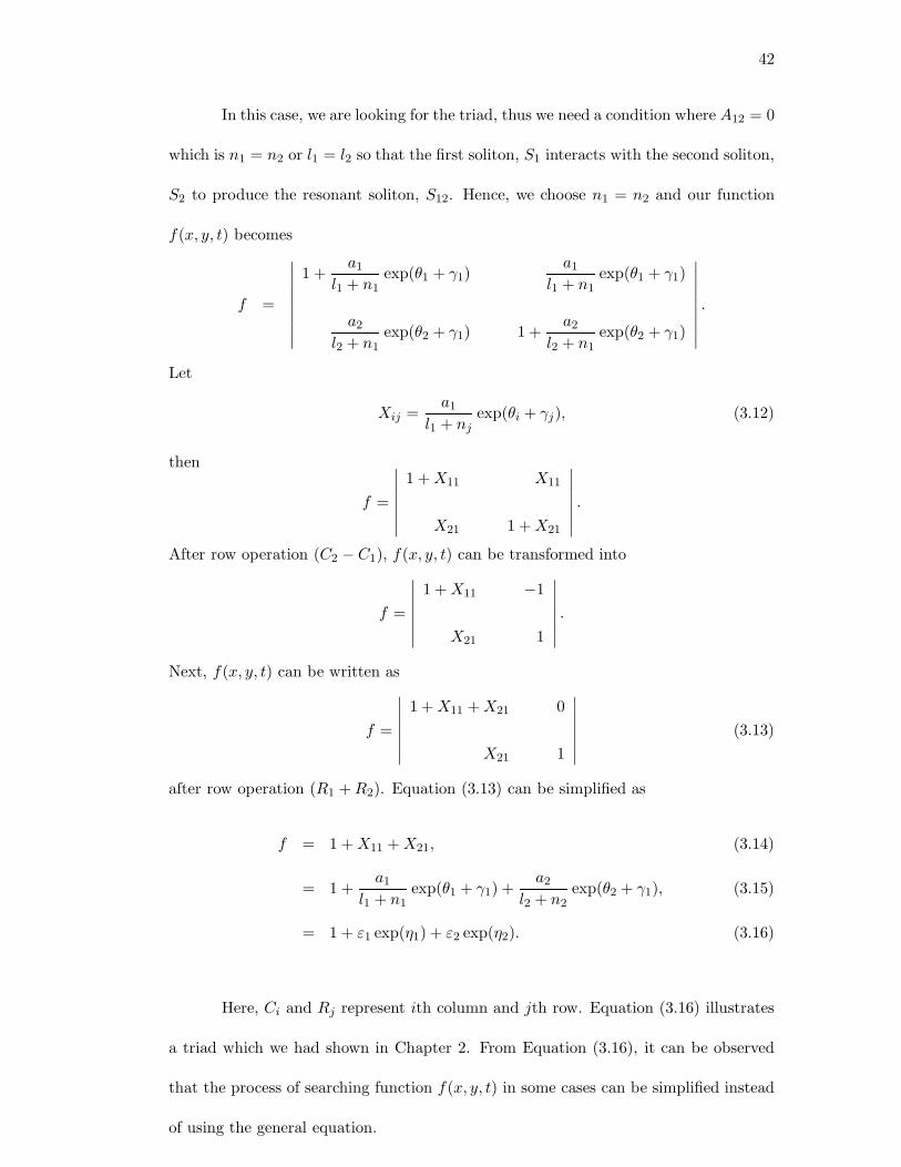
In this case, we are looking for the triad, thus we need a condition where A12 = 0
which is n1 = n2 or l1 = l2 so that the first soliton, S1 interacts with the second soliton,
S2 to produce the resonant soliton, S12. Hence, we choose n1 = n2 and our function
f(x, y, t) becomes
f =
∣∣∣∣∣∣∣∣∣
1 +a1
l1 + n1exp(θ1 + γ1)
a1
l1 + n1exp(θ1 + γ1)
a2
l2 + n1exp(θ2 + γ1) 1 +
a2
l2 + n1exp(θ2 + γ1)
∣∣∣∣∣∣∣∣∣.
Let
Xij =a1
l1 + njexp(θi + γj), (3.12)
then
f =
∣∣∣∣∣∣∣
1 + X11 X11
X21 1 + X21
∣∣∣∣∣∣∣.
After row operation (C2 − C1), f(x, y, t) can be transformed into
f =
∣∣∣∣∣∣∣
1 + X11 −1
X21 1
∣∣∣∣∣∣∣.
Next, f(x, y, t) can be written as
f =
∣∣∣∣∣∣∣
1 + X11 + X21 0
X21 1
∣∣∣∣∣∣∣(3.13)
after row operation (R1 + R2). Equation (3.13) can be simplified as
f = 1 + X11 + X21, (3.14)
= 1 +a1
l1 + n1exp(θ1 + γ1) +
a2
l2 + n2exp(θ2 + γ1), (3.15)
= 1 + ε1 exp(η1) + ε2 exp(η2). (3.16)
Here, Ci and Rj represent ith column and jth row. Equation (3.16) illustrates
a triad which we had shown in Chapter 2. From Equation (3.16), it can be observed
that the process of searching function f(x, y, t) in some cases can be simplified instead
of using the general equation.
43
3.5 Solution For Interaction Between A Triad And A Soliton
We cannot reduced the function f(x, y, t) into Wronskian type in all cases. In
three-soliton interactions, we only can consider the case where a triad interacts with a
soliton. To produce a triad, we have to set a condition which is n1 = n2 6= n3 so that
soliton 1 interacts with soliton 2 in full resonance and produce a triad. Generally the
function f(x, y, t) can be written as
f = | I + X | (3.17)
where I is a identity matrix and X can be written as
X =
a1
l1 + n1eθ1+γ1
a1
l1 + n2eθ1+γ2
a1
l1 + n3eθ1+γ3
a2
l2 + n1eθ2+γ1
a2
l2 + n2eθ2+γ2
a2
l2 + n3eθ2+γ3
a3
l3 + n1eθ3+γ1
a3
l3 + n2eθ3+γ2
a3
l3 + n3eθ3+γ3
(3.18)
After substitution by Equation (3.12), Equation (3.18) becomes
X =
X11 X12 X13
X21 X22 X23
X31 X32 X33
. (3.19)
If we put the condition n1 = n2 6= n3 or γ1 = γ2 6= γ3, the function f(x, y, t) can be
transformed into
f =
∣∣∣∣∣∣∣∣∣∣∣∣
1 + X11 X11 X13
X21 1 + X21 X23
X31 X31 1 + X33
∣∣∣∣∣∣∣∣∣∣∣∣
. (3.20)
By using row operation (C2 − C1), Equation (3.20) becomes
f =
∣∣∣∣∣∣∣∣∣∣∣∣
1 + X11 −1 X13
X21 1 X23
X31 0 1 + X33
∣∣∣∣∣∣∣∣∣∣∣∣
. (3.21)
44
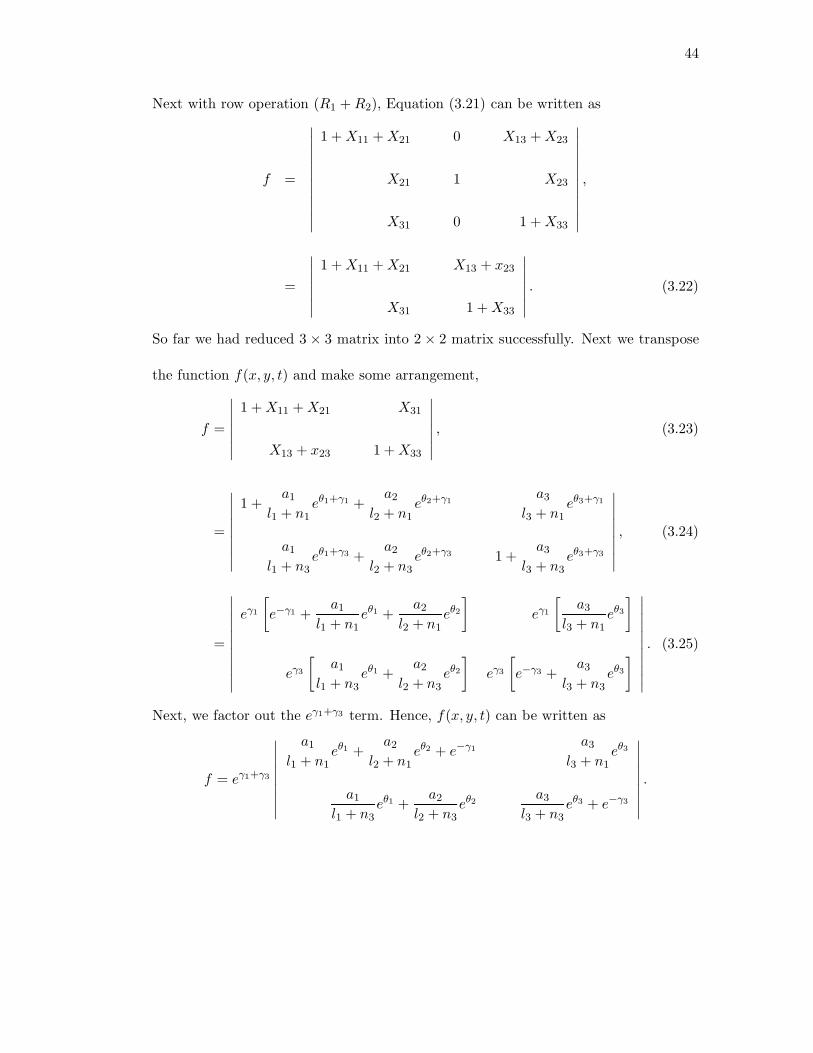
Next with row operation (R1 + R2), Equation (3.21) can be written as
f =
∣∣∣∣∣∣∣∣∣∣∣∣
1 + X11 + X21 0 X13 + X23
X21 1 X23
X31 0 1 + X33
∣∣∣∣∣∣∣∣∣∣∣∣
,
=
∣∣∣∣∣∣∣
1 + X11 + X21 X13 + x23
X31 1 + X33
∣∣∣∣∣∣∣. (3.22)
So far we had reduced 3 × 3 matrix into 2 × 2 matrix successfully. Next we transpose
the function f(x, y, t) and make some arrangement,
f =
∣∣∣∣∣∣∣
1 + X11 + X21 X31
X13 + x23 1 + X33
∣∣∣∣∣∣∣, (3.23)
=
∣∣∣∣∣∣∣∣∣
1 +a1
l1 + n1eθ1+γ1 +
a2
l2 + n1eθ2+γ1
a3
l3 + n1eθ3+γ1
a1
l1 + n3eθ1+γ3 +
a2
l2 + n3eθ2+γ3 1 +
a3
l3 + n3eθ3+γ3
∣∣∣∣∣∣∣∣∣, (3.24)
=
∣∣∣∣∣∣∣∣∣∣∣
eγ1
[e−γ1 +
a1
l1 + n1eθ1 +
a2
l2 + n1eθ2
]eγ1
[a3
l3 + n1eθ3
]
eγ3
[a1
l1 + n3eθ1 +
a2
l2 + n3eθ2
]eγ3
[e−γ3 +
a3
l3 + n3eθ3
]
∣∣∣∣∣∣∣∣∣∣∣
. (3.25)
Next, we factor out the eγ1+γ3 term. Hence, f(x, y, t) can be written as
f = eγ1+γ3
∣∣∣∣∣∣∣∣∣
a1
l1 + n1eθ1 +
a2
l2 + n1eθ2 + e−γ1
a3
l3 + n1eθ3
a1
l1 + n3eθ1 +
a2
l2 + n3eθ2
a3
l3 + n3eθ3 + e−γ3
∣∣∣∣∣∣∣∣∣.
45
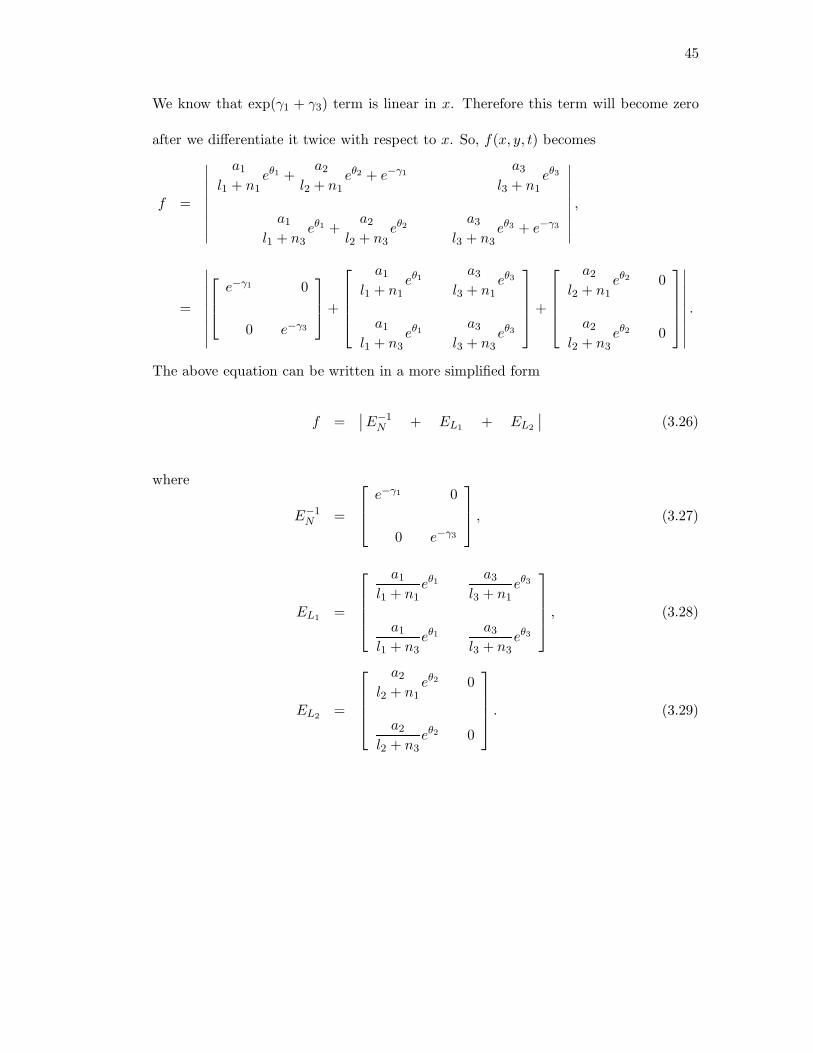
We know that exp(γ1 + γ3) term is linear in x. Therefore this term will become zero
after we differentiate it twice with respect to x. So, f(x, y, t) becomes
f =
∣∣∣∣∣∣∣∣∣
a1
l1 + n1eθ1 +
a2
l2 + n1eθ2 + e−γ1
a3
l3 + n1eθ3
a1
l1 + n3eθ1 +
a2
l2 + n3eθ2
a3
l3 + n3eθ3 + e−γ3
∣∣∣∣∣∣∣∣∣,
=
∣∣∣∣∣∣∣∣∣
e−γ1 0
0 e−γ3
+
a1
l1 + n1eθ1
a3
l3 + n1eθ3
a1
l1 + n3eθ1
a3
l3 + n3eθ3
+
a2
l2 + n1eθ2 0
a2
l2 + n3eθ2 0
∣∣∣∣∣∣∣∣∣.
The above equation can be written in a more simplified form
f =∣∣ E−1
N + EL1 + EL2
∣∣ (3.26)
where
E−1N =
e−γ1 0
0 e−γ3
, (3.27)
EL1 =
a1
l1 + n1eθ1
a3
l3 + n1eθ3
a1
l1 + n3eθ1
a3
l3 + n3eθ3
, (3.28)
EL2 =
a2
l2 + n1eθ2 0
a2
l2 + n3eθ2 0
. (3.29)
46
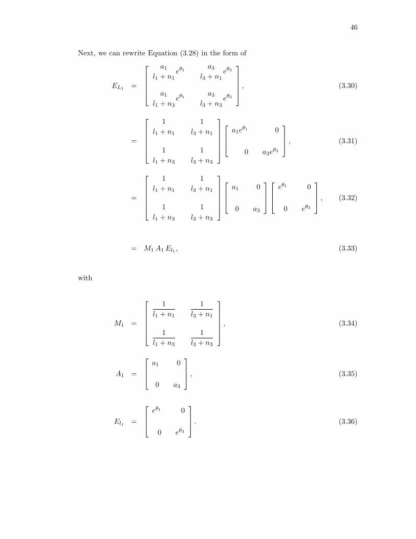
Next, we can rewrite Equation (3.28) in the form of
EL1 =
a1
l1 + n1eθ1
a3
l3 + n1eθ3
a1
l1 + n3eθ1
a3
l3 + n3eθ3
, (3.30)
=
1l1 + n1
1l3 + n1
1l1 + n3
1l3 + n3
a1eθ1 0
0 a3eθ3
, (3.31)
=
1l1 + n1
1l3 + n1
1l1 + n3
1l3 + n3
a1 0
0 a3
eθ1 0
0 eθ3
, (3.32)
= M1 A1 El1 , (3.33)
with
M1 =
1l1 + n1
1l3 + n1
1l1 + n3
1l3 + n3
, (3.34)
A1 =
a1 0
0 a3
, (3.35)
El1 =
eθ1 0
0 eθ3
. (3.36)
47
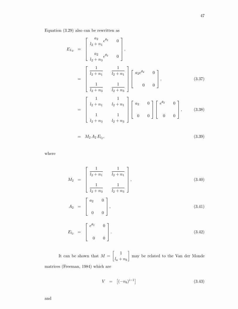
Equation (3.29) also can be rewritten as
EL2 =
a2
l2 + n1eθ2 0
a2
l2 + n3eθ2 0
,
=
1l2 + n1
1l2 + n1
1l2 + n3
1l2 + n3
a2eθ2 0
0 0
, (3.37)
=
1l2 + n1
1l2 + n1
1l2 + n3
1l2 + n3
a2 0
0 0
eθ2 0
0 0
, (3.38)
= M2 A2 El2 , (3.39)
where
M2 =
1l2 + n1
1l2 + n1
1l2 + n3
1l2 + n3
, (3.40)
A2 =
a2 0
0 0
, (3.41)
El2 =
eθ2 0
0 0
. (3.42)
It can be shown that M =[
1la + nb
]may be related to the Van der Monde
matrices (Freeman, 1984) which are
V =[(−nb)i−1
](3.43)
and
48
W =[(−1)j−1(la)i−1
]. (3.44)
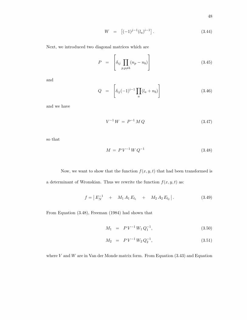
Next, we introduced two diagonal matrices which are
P =
δij
∏
p,p 6=b
(np − nb)
(3.45)
and
Q =
[δij(−1)i−1
∏
a
(la + nb)
](3.46)
and we have
V −1 W = P−1 M Q (3.47)
so that
M = P V −1 W Q−1 (3.48)
Now, we want to show that the function f(x, y, t) that had been transformed is
a determinant of Wronskian. Thus we rewrite the function f(x, y, t) as:
f =∣∣ E−1
N + M1 A1 El1 + M2 A2 El2
∣∣ . (3.49)
From Equation (3.48), Freeman (1984) had shown that
M1 = P V −1 W1 Q−11 , (3.50)
M2 = P V −1 W2 Q−12 , (3.51)
where V and W are in Van der Monde matrix form. From Equation (3.43) and Equation
49
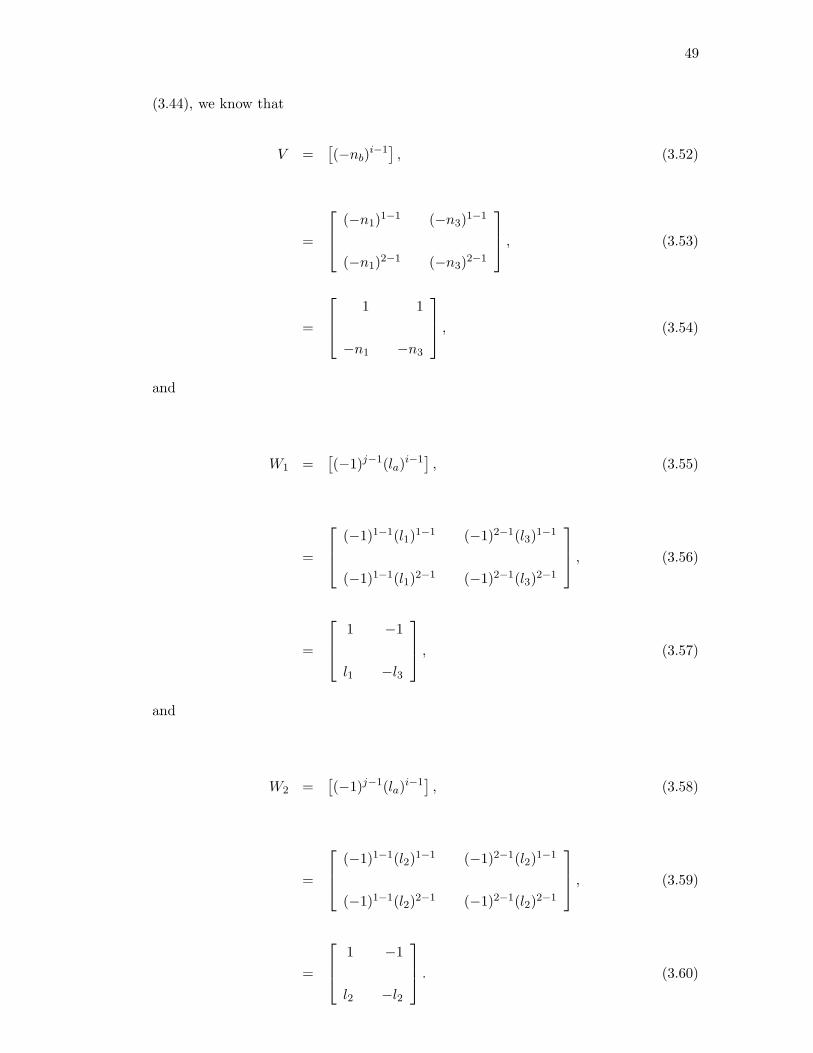
(3.44), we know that
V =[(−nb)i−1
], (3.52)
=
(−n1)1−1 (−n3)1−1
(−n1)2−1 (−n3)2−1
, (3.53)
=
1 1
−n1 −n3
, (3.54)
and
W1 =[(−1)j−1(la)i−1
], (3.55)
=
(−1)1−1(l1)1−1 (−1)2−1(l3)1−1
(−1)1−1(l1)2−1 (−1)2−1(l3)2−1
, (3.56)
=
1 −1
l1 −l3
, (3.57)
and
W2 =[(−1)j−1(la)i−1
], (3.58)
=
(−1)1−1(l2)1−1 (−1)2−1(l2)1−1
(−1)1−1(l2)2−1 (−1)2−1(l2)2−1
, (3.59)
=
1 −1
l2 −l2
. (3.60)
50
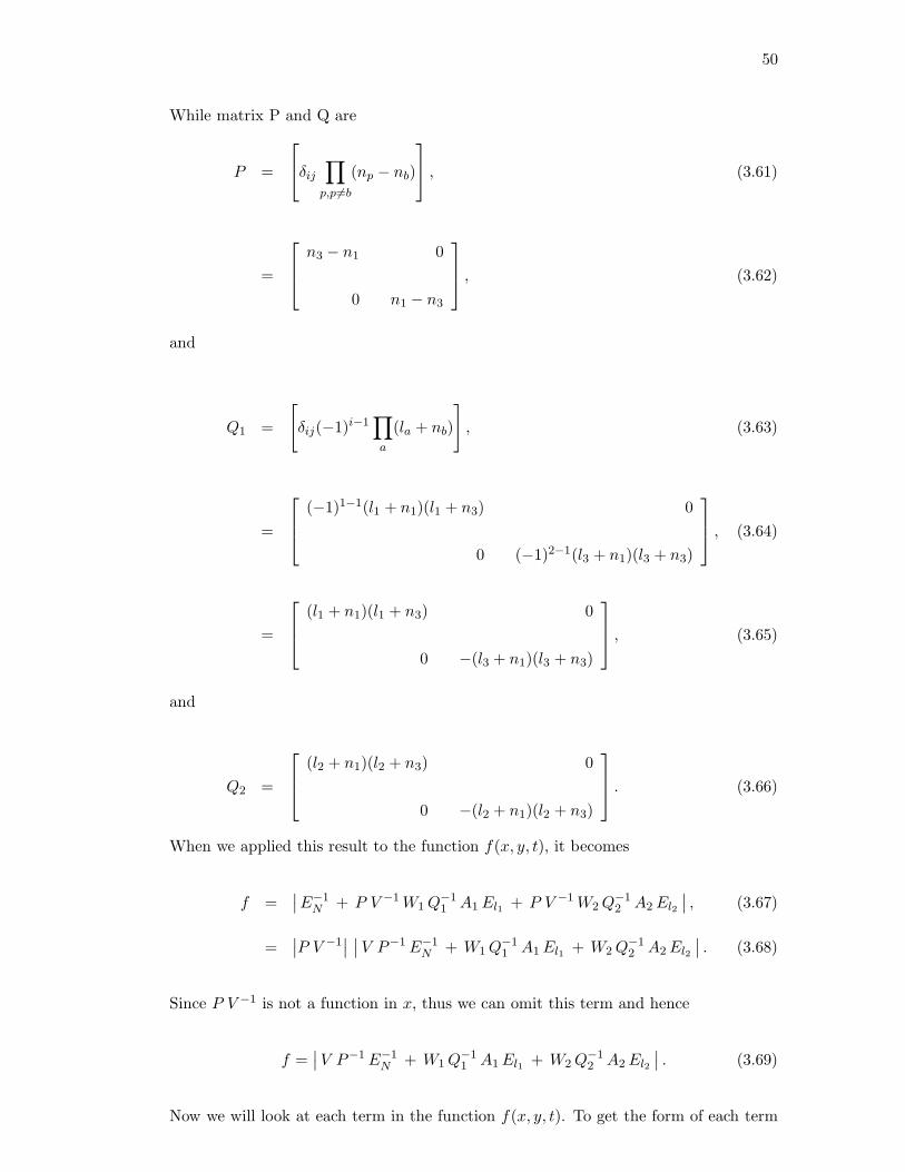
While matrix P and Q are
P =
δij
∏
p,p 6=b
(np − nb)
, (3.61)
=
n3 − n1 0
0 n1 − n3
, (3.62)
and
Q1 =
[δij(−1)i−1
∏
a
(la + nb)
], (3.63)
=
(−1)1−1(l1 + n1)(l1 + n3) 0
0 (−1)2−1(l3 + n1)(l3 + n3)
, (3.64)
=
(l1 + n1)(l1 + n3) 0
0 −(l3 + n1)(l3 + n3)
, (3.65)
and
Q2 =
(l2 + n1)(l2 + n3) 0
0 −(l2 + n1)(l2 + n3)
. (3.66)
When we applied this result to the function f(x, y, t), it becomes
f =∣∣E−1
N + P V −1 W1 Q−11 A1 El1 + P V −1 W2 Q−1
2 A2 El2
∣∣ , (3.67)
=∣∣P V −1
∣∣ ∣∣ V P−1 E−1N + W1 Q−1
1 A1 El1 + W2 Q−12 A2 El2
∣∣ . (3.68)
Since P V −1 is not a function in x, thus we can omit this term and hence
f =∣∣ V P−1 E−1
N + W1 Q−11 A1 El1 + W2 Q−1
2 A2 El2
∣∣ . (3.69)
Now we will look at each term in the function f(x, y, t). To get the form of each term
51
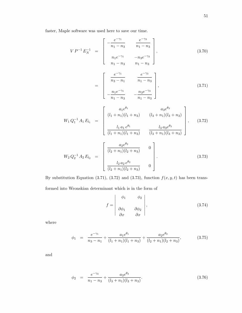
faster, Maple software was used here to save our time.
V P−1 E−1N =
− e−γ1
n1 − n3
e−γ3
n1 − n3
n1e−γ1
n1 − n3
−n3e−γ3
n1 − n3
, (3.70)
=
e−γ1
n3 − n1
e−γ3
n1 − n3
− n1e−γ1
n1 − n3− n3e
−γ3
n1 − n3
, (3.71)
W1 Q−11 A1 El1 =
a1eθ1
(l1 + n1)(l1 + n3)a3e
θ3
(l3 + n1)(l3 + n3)
l1 a1 eθ1
(l1 + n1)(l1 + n3)l3 a3e
θ3
(l3 + n1)(l3 + n3)
, (3.72)
W2 Q−12 A2 El2 =
a2eθ2
(l2 + n1)(l2 + n3)0
l2 a2 eθ2
(l2 + n1)(l2 + n3)0
. (3.73)
By substitution Equation (3.71), (3.72) and (3.73), function f(x, y, t) has been trans-
formed into Wronskian determinant which is in the form of
f =
∣∣∣∣∣∣∣∣
φ1 φ2
∂φ1
∂x
∂φ2
∂x
∣∣∣∣∣∣∣∣, (3.74)
where
φ1 =e−γ1
n3 − n1+
a1eθ1
(l1 + n1)(l1 + n3)+
a2eθ2
(l2 + n1)(l2 + n3), (3.75)
and
φ2 =e−γ3
n1 − n3+
a3eθ3
(l3 + n1)(l3 + n3). (3.76)
52
3.6 Computer Simulation
In this section, illustration of the interactions of three solitons are shown. The
codes of KPPRO which is the computer program to simulate the three solitons inter-
actions are included in the Appendix A.
3.6.1 A Triad Interacts With A Soliton
We have three types of interactions for the interactions between a triad with a
soliton which are n1 = n2 ≈ n3, n2 = n3 ≈ n1 and n1 = n3 ≈ n2 respectively.
3.6.1.1 Type 1: n1 = n2 ≈ n3
From the previous section, we have shown that the function f(x, y, t) for inter-
action of a triad with a soliton can be simplified into Wronskian determinant. Thus,
before we discuss more about the illustration of the interactions, let us look at the
function f(x, y, t) which will govern the interaction. From Equation (3.74), (3.75) and
(3.76), we know that
f =
∣∣∣∣∣∣∣∣∣∣∣
e−γ1
n3 − n1+
a1eθ1
(l1 + n1)(l1 + n3)+
a2eθ2
(l2 + n1)(l2 + n3)eγ3
n1 − n3+
a3eθ3
(l3 + n1)(l3 + n3)
−n1e−γ1
n3 − n1+
a1l1eθ1
(l1 + n1)(l1 + n3)+
a2l2eθ2
(l2 + n1)(l2 + n3)−n3e
−γ3
n1 − n3+
a3l3eθ3
(l3 + n1)(l3 + n3)
∣∣∣∣∣∣∣∣∣∣∣
,
53
f =[(
e−γ1
n3 − n1+
a1eθ1
(l1 + n1)(l1 + n3)+
a2eθ2
(l2 + n1)(l2 + n3)
)
(−n3e
−γ3
n1 − n3+
a3l3eθ3
(l3 + n1)(l3 + n3)
)
−(−n1e
−γ1
n3 − n1+
a1l1eθ1
(l1 + n1)(l1 + n3)+
a2l2eθ2
(l2 + n1)(l2 + n3)
)
(eγ3
n1 − n3+
a3eθ3
(l3 + n1)(l3 + n3)
)],
f =(−n3 + n1)e−γ1−γ3
(n3 − n1)(n1 − n3)+
(l3 + n1)a3e−γ1+θ3
(n3 − n1)(l3 + n1)(l3 + n3)
− (n3 + l1)a1e−γ3+θ1
(n1 − n3)(l1 + n1)(l1 + n3)+
(l3 − l1)a1a3eθ1+θ3
(l1 + n1)(l1 + n3)(l3 + n1)(l3 + n3)
− (n3 + l2)a2e−γ3+θ2
(l2 + n1)(l2 + n3)(n1 − n3)+
(l3 + l2)a2a3eθ2+θ3
(l2 + n1)(l2 + n3)(l3 + n1)(l3 + n3).
Let εi =ai
li + niand make some simplification, the above equation becomes
f =e−γ1−γ3
(n3 − n1)+
ε3eγ1+θ3
(n3 − n1)− ε1e
−γ3+θ1
(n1 − n3)+
(l3 − l1)ε1ε3eθ1+θ3
(l1 + n3)(l3 + n1)
− a2e−γ3+θ2
(l2 + n1)(n1 − n3)+
(l3 − l2)a2ε3eθ2+θ3
(l2 + n1)(l2 + n3)(l3 + n1). (3.77)
Multiply Equation (3.77) with (n3 − n1), then f(x, y, t) becomes
f = e−γ1−γ3 + ε3eγ1+θ3 + ε1e
−γ3+θ1 +(l3 − l1)(n3 − n1)ε1ε3e
θ1+θ3
(l1 + n3)(l3 + n1)
+a2e
−γ3+θ2
(l2 + n1)+
(l3 + l2)(n3 − n1)a2ε3eθ2+θ3
(l2 + n1)(l2 + n3)(l3 + n1). (3.78)
Next, we multiply the function f(x, y, t) with eγ1
f = e−γ3 + ε3eθ3 + ε1e
γ1−γ3+θ1 +(l3 − l1)(n3 − n1)ε1ε3e
γ1+θ1+θ3
(l1 + n3)(l3 + n1)
+a2e
γ1−γ3+θ2
(l2 + n1)+
(l3 + l2)(n3 − n1)a2ε3eγ1+θ2+θ3
(l2 + n1)(l2 + n3)(l3 + n1). (3.79)
After that, multiply again Equation (3.79) with eγ3
f = 1 + ε3eγ3+θ3 + ε1e
γ1+θ1 +(l3 − l1)(n3 − n1)ε1ε3e
γ1+θ1+γ3+θ3
(l1 + n3)(l3 + n1)
+a2e
γ1+θ2
(l2 + n1)+
(l3 + l2)(n3 − n1)a2ε3eγ1+θ2+γ3+θ3
(l2 + n1)(l2 + n3)(l3 + n1). (3.80)
54
From Equation (3.9), we had stated that ηi = θi + γi, thus Equation (3.80) can be
rewritten as
f = 1 + ε3eη3 + ε1e
η1 +(l3 − l1)(n3 − n1)ε1ε3e
η1+η3
(l1 + n3)(l3 + n1)
+a2e
γ1+θ2
(l2 + n1)+
(l3 + l2)(n3 − n1)a2ε3eγ1+θ2+η3
(l2 + n1)(l2 + n3)(l3 + n1). (3.81)
For this case, we had set the condition which is n1 = n2 or γ1 = γ2, therefore Equation
(3.81) becomes
f = 1 + ε3eη3 + ε1e
η1 +(l3 − l1)(n3 − n1)ε1ε3e
η1+η3
(l1 + n3)(l3 + n1)
+ ε2eη2 +
(l3 − l2)(n3 − n2)ε2ε3eη2+η3
(l2 + n3)(l3 + n2), (3.82)
f = 1 + ε1eη1 + ε2e
η2 + ε3eη3 + A13ε1ε3e
η1+η3 + A23ε2ε3eη2+η3 (3.83)
where
A13 =(l1 + l3)(n1 + n3)l1 + n3)(l3 + n1)
, (3.84)
A23 =(l2 + l3)(n2 + n3)l2 + n3)(l3 + n2)
, (3.85)
or we can conclude that
Aij =(li + lj)(ni + nj)li + nj)(lj + ni)
. (3.86)
Now we want to discuss the interaction between a triad and a soliton. For this
purpose we will use KPPRO. The following is the series of picture about the interactions
of three KP solitons, where a triad interacts with a soliton.
For this case the values of parameter were chosen as follow where soliton 1, S1
and soliton 2, S2 will be in full resonance (n1 = n2 = 3) and we also choose n3 to be
very close to n1, n2 so that it will then go into resonance process with the other two
55
solitons.
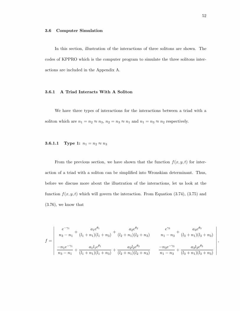
n1 = 3 n2 = 3 n3 = 3 + 10−11
l1 = −2 l2 = 3 l3 = 2 (3.87)
Figure 3.1: A triad interacts with a soliton at t = 0.5s
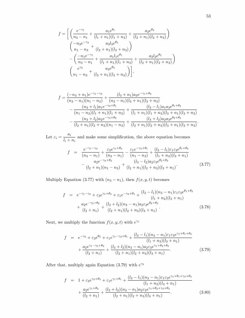
S1
S2
S12S3
12
13
2314
.................................................................
.................................................................
.................................................................
.
.............................................................................................................................................
........................................................................................................................................................................................................................................................................................................................................................................................................................................
.................................................................................................................................................................................................................................................................................................................................................................................................................................................................................................................................
Figure 3.2: Geometrical representation of a triad interacts with a soliton at t = 0.5s
56
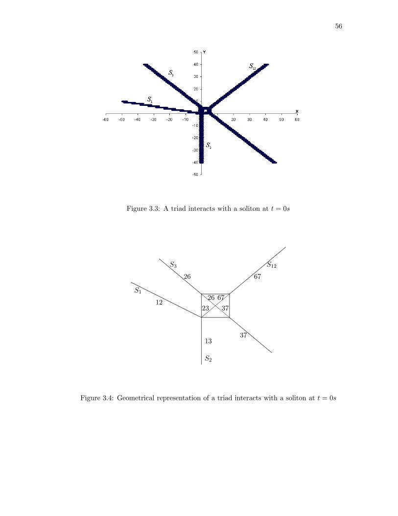
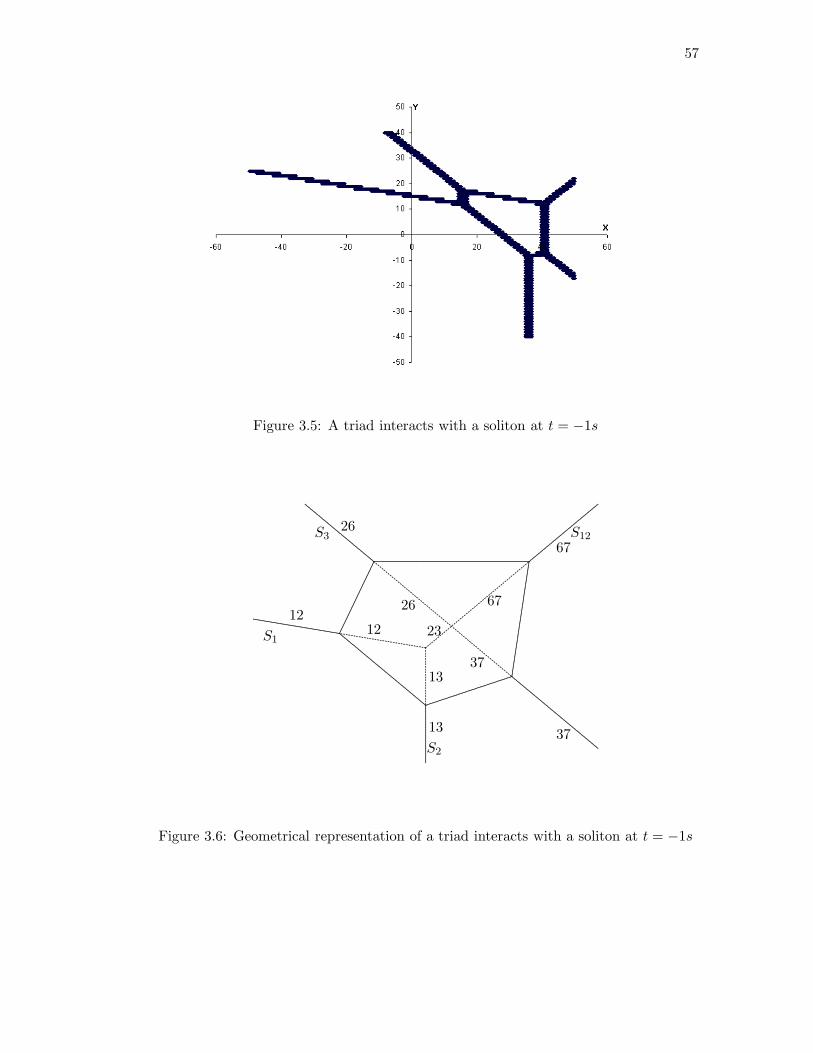
Figure 3.3: A triad interacts with a soliton at t = 0s
S1
S2
S12S3
12
13
6726
2326
3767
37
....................................
...................................
...................................
....................................
....................................
...................................
...................................
...................................
.....................
................................................................................................................................................................................................................................................................................
.................................................................................................................................................................................................................................................................................................................................
.........................
.........................
........................
.........................
..........................
.........................
.........................
.........................
....................................................................................................................................................................................................................
...........................................................................................................................................................................................................................................................................................
............................................................................................................................................................................
Figure 3.4: Geometrical representation of a triad interacts with a soliton at t = 0s
57
Figure 3.5: A triad interacts with a soliton at t = −1s
S3
S2
S12
S112
12
13
13
67
26
23
26
67
37
37
........
........
........
........
........
........
........
........
........
........
........
........
........
..........................................
.................................................
..................................................
........................................................................................................................................................................................................................................................
........
........
........
........
........
........
........
........
........
........
........
........
........
........
........
........
........
........
........
........
........
........
........
........
........
........
........
....................................................................................................................................................................................................................................................................................................................................................................................................................................................................................................................................................................................................................................................................................
..............................................................................................
.......................................................................
.........................
.........................
.........................
..........................
.........................
........................
....................
..........................................................................................................................................................................
..................................................................
.........................................................
..........................................
.....................................................................................................................................................................................................................................................................................................................................................................
Figure 3.6: Geometrical representation of a triad interacts with a soliton at t = −1s
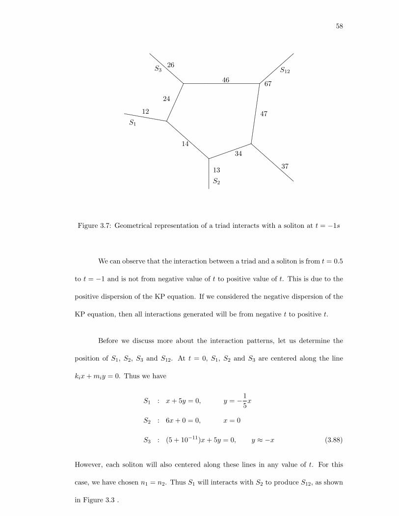
58
S3
S2
S12
S1
12
13
67
26
14
24
46
47
34
37
........
........
........
........
........
........
........
........
........
........
........
........
........
........
..........................................
...............................................
..............................................
....................................................................................................................................................................................................................................................................
........
........
........
........
........
........
........
........
........
........
........
........
........
........
........
........
........
........
........
........
........
........
........
........
........
........
........
........
........
................................................................................................................................................................................................................................................................................................................................................................................................................................................................................................................................................................................................................................................................................................
..........................................................................................
............................................................................
........................
........................
........................
........................
........................
........................
........................
.......
...............................................................................................................................................................................
Figure 3.7: Geometrical representation of a triad interacts with a soliton at t = −1s
We can observe that the interaction between a triad and a soliton is from t = 0.5
to t = −1 and is not from negative value of t to positive value of t. This is due to the
positive dispersion of the KP equation. If we considered the negative dispersion of the
KP equation, then all interactions generated will be from negative t to positive t.
Before we discuss more about the interaction patterns, let us determine the
position of S1, S2, S3 and S12. At t = 0, S1, S2 and S3 are centered along the line
kix + miy = 0. Thus we have
S1 : x + 5y = 0, y = −15x
S2 : 6x + 0 = 0, x = 0
S3 : (5 + 10−11)x + 5y = 0, y ≈ −x (3.88)
However, each soliton will also centered along these lines in any value of t. For this
case, we have chosen n1 = n2. Thus S1 will interacts with S2 to produce S12, as shown
in Figure 3.3 .
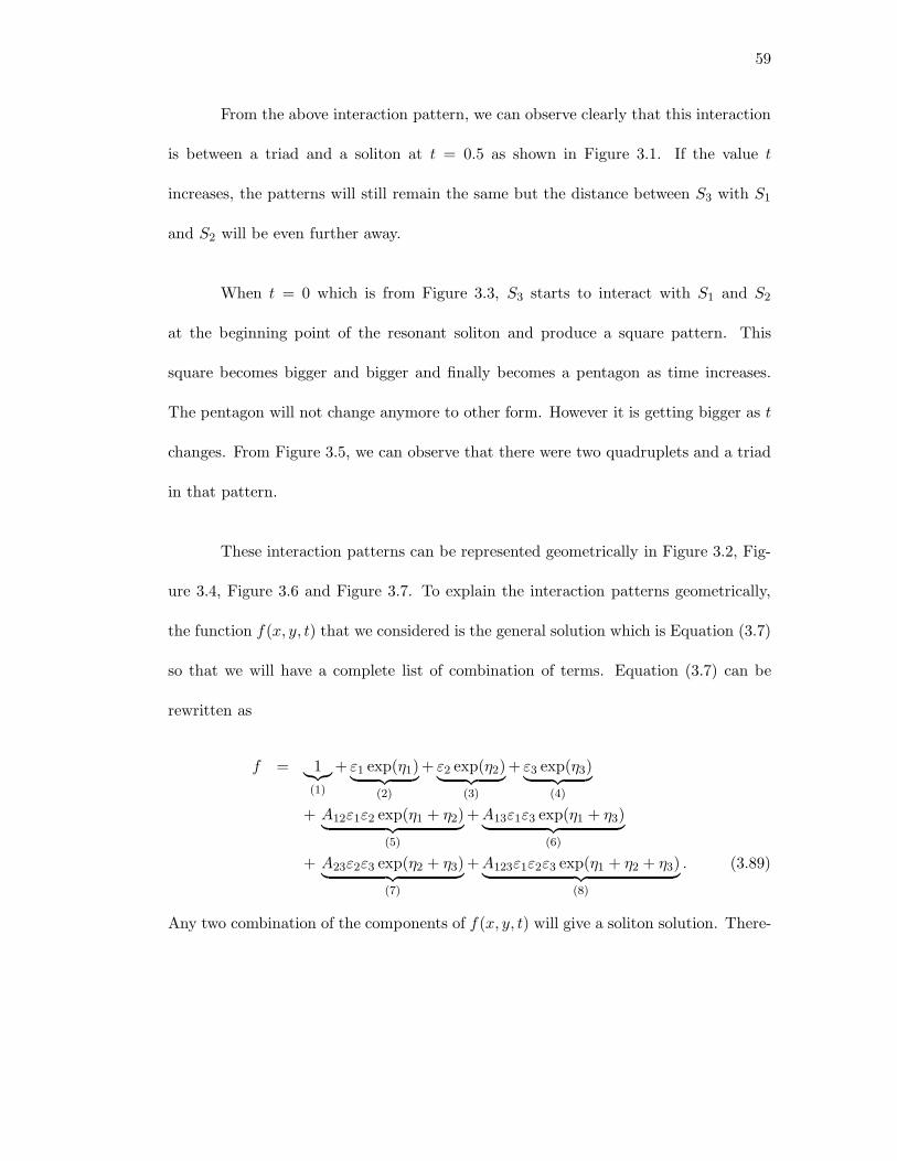
59
From the above interaction pattern, we can observe clearly that this interaction
is between a triad and a soliton at t = 0.5 as shown in Figure 3.1. If the value t
increases, the patterns will still remain the same but the distance between S3 with S1
and S2 will be even further away.
When t = 0 which is from Figure 3.3, S3 starts to interact with S1 and S2
at the beginning point of the resonant soliton and produce a square pattern. This
square becomes bigger and bigger and finally becomes a pentagon as time increases.
The pentagon will not change anymore to other form. However it is getting bigger as t
changes. From Figure 3.5, we can observe that there were two quadruplets and a triad
in that pattern.
These interaction patterns can be represented geometrically in Figure 3.2, Fig-
ure 3.4, Figure 3.6 and Figure 3.7. To explain the interaction patterns geometrically,
the function f(x, y, t) that we considered is the general solution which is Equation (3.7)
so that we will have a complete list of combination of terms. Equation (3.7) can be
rewritten as
f = 1︸︷︷︸(1)
+ ε1 exp(η1)︸ ︷︷ ︸(2)
+ ε2 exp(η2)︸ ︷︷ ︸(3)
+ ε3 exp(η3)︸ ︷︷ ︸(4)
+ A12ε1ε2 exp(η1 + η2)︸ ︷︷ ︸(5)
+A13ε1ε3 exp(η1 + η3)︸ ︷︷ ︸(6)
+ A23ε2ε3 exp(η2 + η3)︸ ︷︷ ︸(7)
+A123ε1ε2ε3 exp(η1 + η2 + η3)︸ ︷︷ ︸(8)
. (3.89)
Any two combination of the components of f(x, y, t) will give a soliton solution. There-
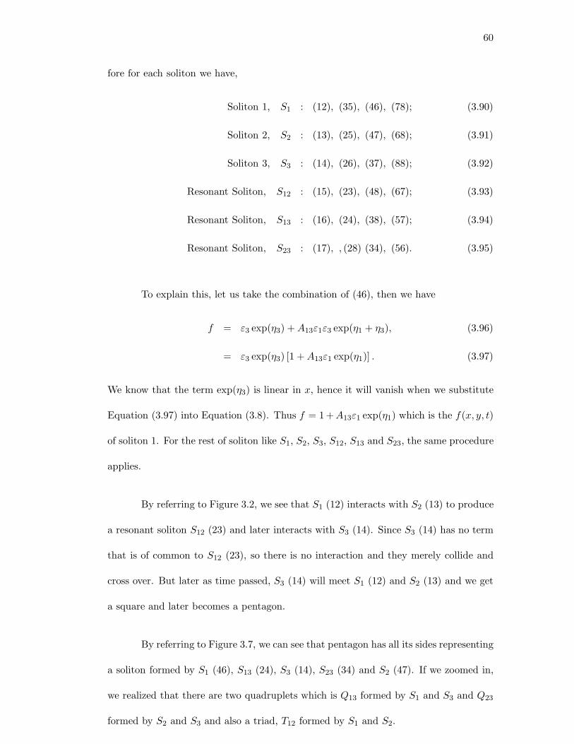
60
fore for each soliton we have,
Soliton 1, S1 : (12), (35), (46), (78); (3.90)
Soliton 2, S2 : (13), (25), (47), (68); (3.91)
Soliton 3, S3 : (14), (26), (37), (88); (3.92)
Resonant Soliton, S12 : (15), (23), (48), (67); (3.93)
Resonant Soliton, S13 : (16), (24), (38), (57); (3.94)
Resonant Soliton, S23 : (17), , (28) (34), (56). (3.95)
To explain this, let us take the combination of (46), then we have
f = ε3 exp(η3) + A13ε1ε3 exp(η1 + η3), (3.96)
= ε3 exp(η3) [1 + A13ε1 exp(η1)] . (3.97)
We know that the term exp(η3) is linear in x, hence it will vanish when we substitute
Equation (3.97) into Equation (3.8). Thus f = 1 +A13ε1 exp(η1) which is the f(x, y, t)
of soliton 1. For the rest of soliton like S1, S2, S3, S12, S13 and S23, the same procedure
applies.
By referring to Figure 3.2, we see that S1 (12) interacts with S2 (13) to produce
a resonant soliton S12 (23) and later interacts with S3 (14). Since S3 (14) has no term
that is of common to S12 (23), so there is no interaction and they merely collide and
cross over. But later as time passed, S3 (14) will meet S1 (12) and S2 (13) and we get
a square and later becomes a pentagon.
By referring to Figure 3.7, we can see that pentagon has all its sides representing
a soliton formed by S1 (46), S13 (24), S3 (14), S23 (34) and S2 (47). If we zoomed in,
we realized that there are two quadruplets which is Q13 formed by S1 and S3 and Q23
formed by S2 and S3 and also a triad, T12 formed by S1 and S2.
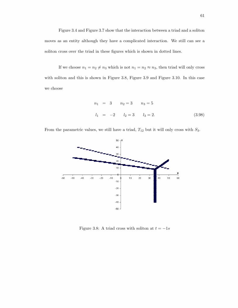
61
Figure 3.4 and Figure 3.7 show that the interaction between a triad and a soliton
moves as an entity although they have a complicated interaction. We still can see a
soliton cross over the triad in these figures which is shown in dotted lines.
If we choose n1 = n2 6= n3 which is not n1 = n2 ≈ n3, then triad will only cross
with soliton and this is shown in Figure 3.8, Figure 3.9 and Figure 3.10. In this case
we choose
n1 = 3 n2 = 3 n3 = 5
l1 = −2 l2 = 3 l3 = 2. (3.98)
From the parametric values, we still have a triad, T12 but it will only cross with S3.
Figure 3.8: A triad cross with soliton at t = −1s
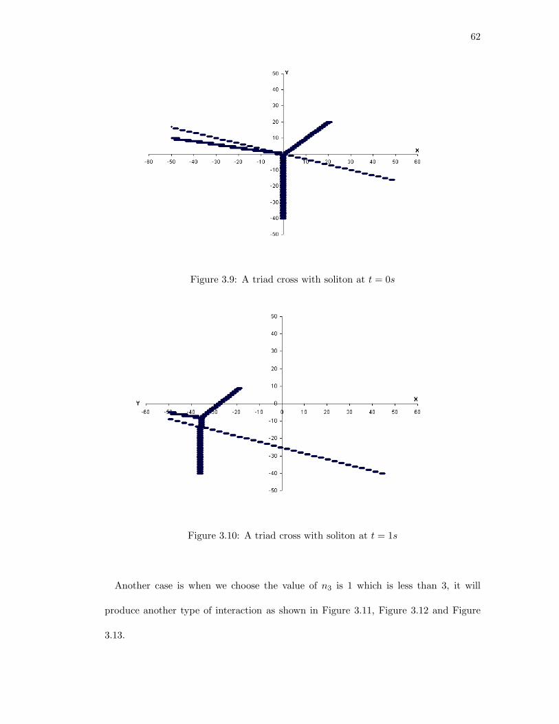
62
Figure 3.9: A triad cross with soliton at t = 0s
Figure 3.10: A triad cross with soliton at t = 1s
Another case is when we choose the value of n3 is 1 which is less than 3, it will
produce another type of interaction as shown in Figure 3.11, Figure 3.12 and Figure
3.13.
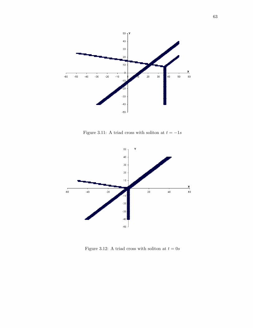
63
Figure 3.11: A triad cross with soliton at t = −1s
Figure 3.12: A triad cross with soliton at t = 0s
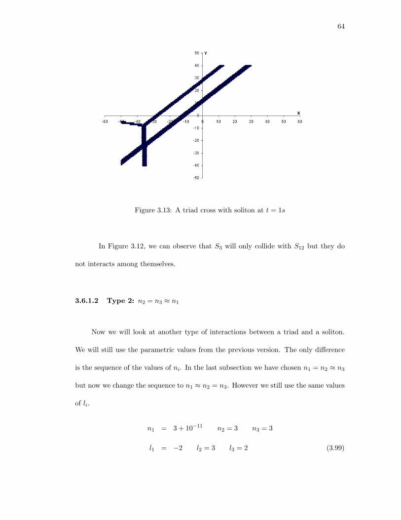
64
Figure 3.13: A triad cross with soliton at t = 1s
In Figure 3.12, we can observe that S3 will only collide with S12 but they do
not interacts among themselves.
3.6.1.2 Type 2: n2 = n3 ≈ n1
Now we will look at another type of interactions between a triad and a soliton.
We will still use the parametric values from the previous version. The only difference
is the sequence of the values of ni. In the last subsection we have chosen n1 = n2 ≈ n3
but now we change the sequence to n1 ≈ n2 = n3. However we still use the same values
of li.
n1 = 3 + 10−11 n2 = 3 n3 = 3
l1 = −2 l2 = 3 l3 = 2 (3.99)
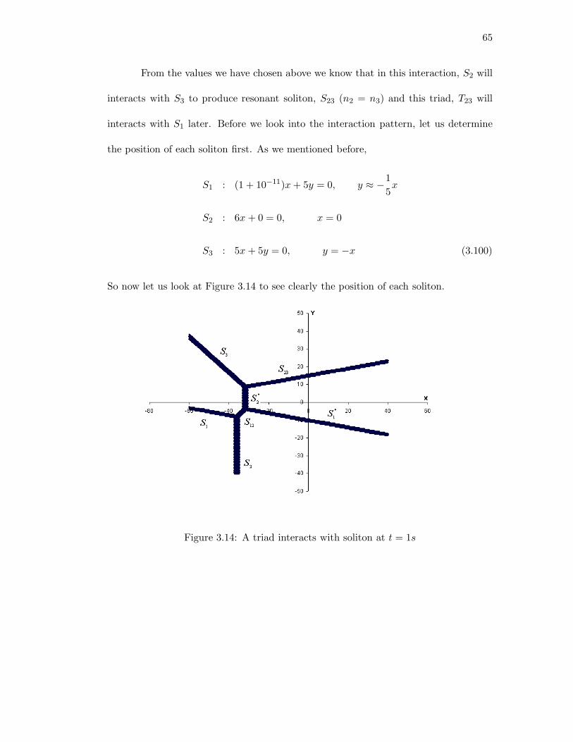
65
From the values we have chosen above we know that in this interaction, S2 will
interacts with S3 to produce resonant soliton, S23 (n2 = n3) and this triad, T23 will
interacts with S1 later. Before we look into the interaction pattern, let us determine
the position of each soliton first. As we mentioned before,
S1 : (1 + 10−11)x + 5y = 0, y ≈ −15x
S2 : 6x + 0 = 0, x = 0
S3 : 5x + 5y = 0, y = −x (3.100)
So now let us look at Figure 3.14 to see clearly the position of each soliton.
Figure 3.14: A triad interacts with soliton at t = 1s
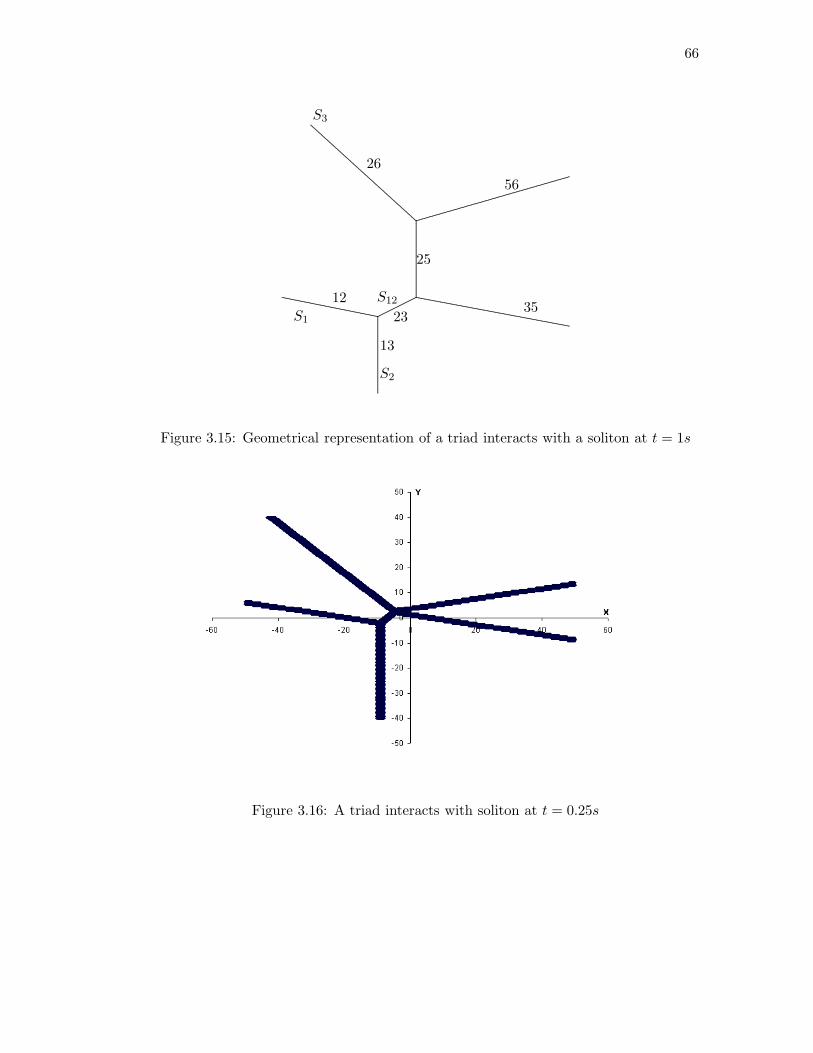
66
S3
S2
S12
S1
12
13
56
25
23
26
35
........
........
........
........
........
........
........
........
........
........
........
........
........
........
........
........
........
........
.................................................................................
................................................................................
.........................
....................................
....................................
................................................................................................................................................................................................................................................................................................................
........
........
........
........
........
........
........
........
........
........
........
........
........
........
........
........
........
........
..........................................................
........................................................
.........................................................
........................................................
.........................................................
..................
........................
........................
........................
........................
........................
........................
........................
........................
........................
........................
........................
.....
Figure 3.15: Geometrical representation of a triad interacts with a soliton at t = 1s
Figure 3.16: A triad interacts with soliton at t = 0.25s
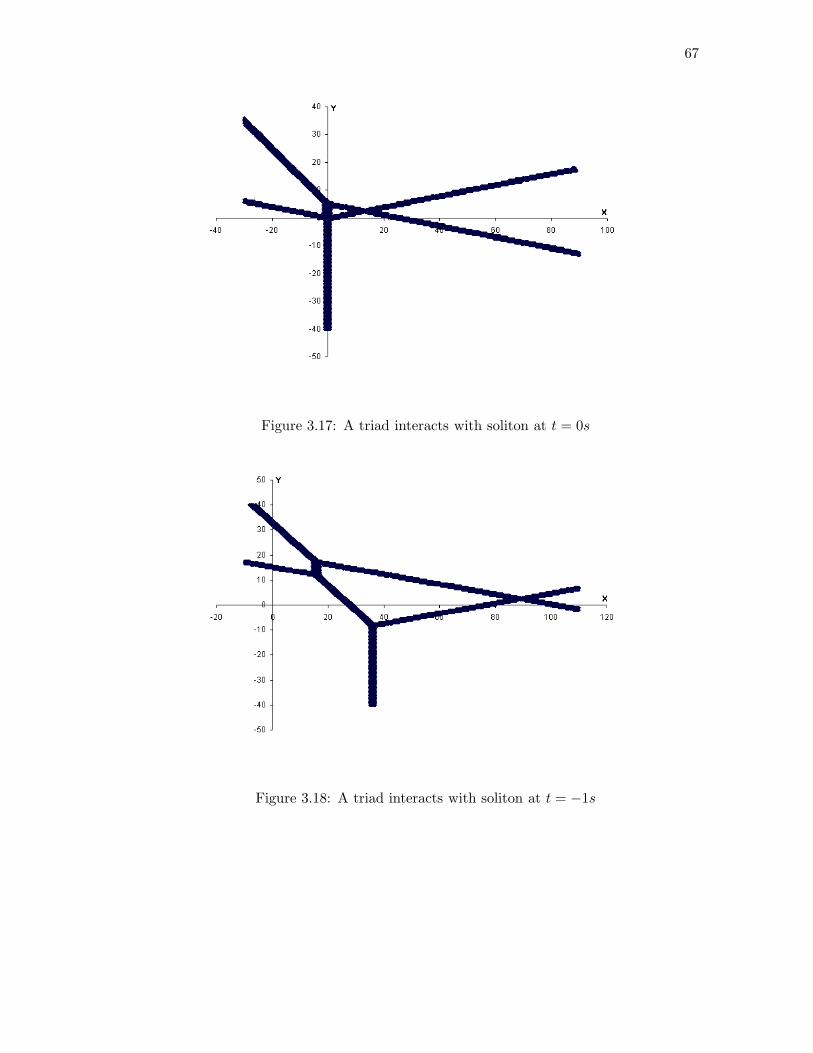
67
Figure 3.17: A triad interacts with soliton at t = 0s
Figure 3.18: A triad interacts with soliton at t = −1s
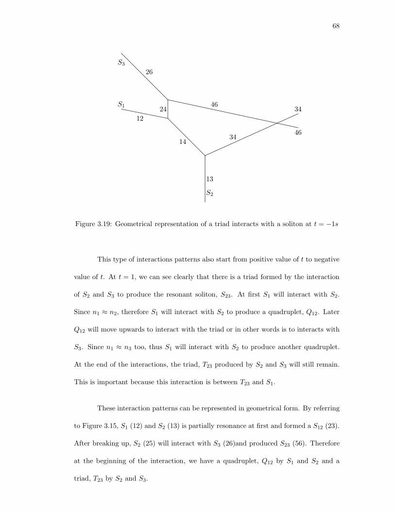
68
S3
S2
S1
12
13
14
24 34
34
26
46
46
........
........
........
........
........
........
........
........
........
........
........
........
........
........
........
........
........
........
........
........
........
........
.................................
......................................
.......................................
......................................
.......................................
......................................
.......................................
......................................
.......................................
......................................
.......................
.......................
......................
.......................
.......................
......................
.......................
.......................
......................
.......................
.................................................................................
................................................................................
.........................
........
........
........
........
........
........
........
........
........
........................
......................
.......................
.......................
......................
.......................
.......................
......................
.......................
.......................
......................
.......
......................................................................................................................................................................................................................................................................................................................................................................................................................................................................................................................................
Figure 3.19: Geometrical representation of a triad interacts with a soliton at t = −1s
This type of interactions patterns also start from positive value of t to negative
value of t. At t = 1, we can see clearly that there is a triad formed by the interaction
of S2 and S3 to produce the resonant soliton, S23. At first S1 will interact with S2.
Since n1 ≈ n2, therefore S1 will interact with S2 to produce a quadruplet, Q12. Later
Q12 will move upwards to interact with the triad or in other words is to interacts with
S3. Since n1 ≈ n3 too, thus S1 will interact with S2 to produce another quadruplet.
At the end of the interactions, the triad, T23 produced by S2 and S3 will still remain.
This is important because this interaction is between T23 and S1.
These interaction patterns can be represented in geometrical form. By referring
to Figure 3.15, S1 (12) and S2 (13) is partially resonance at first and formed a S12 (23).
After breaking up, S2 (25) will interact with S3 (26)and produced S23 (56). Therefore
at the beginning of the interaction, we have a quadruplet, Q12 by S1 and S2 and a
triad, T23 by S2 and S3.
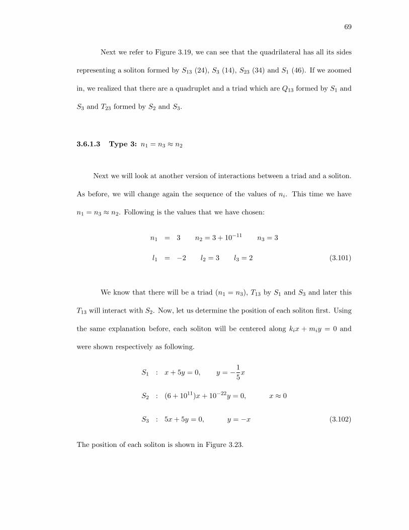
69
Next we refer to Figure 3.19, we can see that the quadrilateral has all its sides
representing a soliton formed by S13 (24), S3 (14), S23 (34) and S1 (46). If we zoomed
in, we realized that there are a quadruplet and a triad which are Q13 formed by S1 and
S3 and T23 formed by S2 and S3.
3.6.1.3 Type 3: n1 = n3 ≈ n2
Next we will look at another version of interactions between a triad and a soliton.
As before, we will change again the sequence of the values of ni. This time we have
n1 = n3 ≈ n2. Following is the values that we have chosen:
n1 = 3 n2 = 3 + 10−11 n3 = 3
l1 = −2 l2 = 3 l3 = 2 (3.101)
We know that there will be a triad (n1 = n3), T13 by S1 and S3 and later this
T13 will interact with S2. Now, let us determine the position of each soliton first. Using
the same explanation before, each soliton will be centered along kix + miy = 0 and
were shown respectively as following.
S1 : x + 5y = 0, y = −15x
S2 : (6 + 1011)x + 10−22y = 0, x ≈ 0
S3 : 5x + 5y = 0, y = −x (3.102)
The position of each soliton is shown in Figure 3.23.
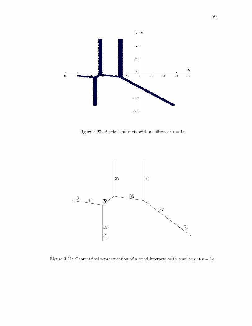
70
Figure 3.20: A triad interacts with a soliton at t = 1s
S3
S2
S1 12
13
23
25
35
57
37
........
........
........
........
........
........
........
........
........
........
........
........
........
........
........
........
........
........
........
........
........
........
........
........
........
........
........
............................................................................................
........................................................................................................
...............................................................................
........
........
........
........
........
........
........
........
........
........
........
........
........
........
........
........
........
........
........
........
........
........
........
........
........
........
........
.
.................................................................................................................................................................................................................................................................................................................................................................................................................................................................................................................................................................
........
........
........
........
........
........
........
........
........
........
........
........
........
........
........
........
........
........
........
........
........
........
........
........
........
........
........
........
........
........
....
Figure 3.21: Geometrical representation of a triad interacts with a soliton at t = 1s
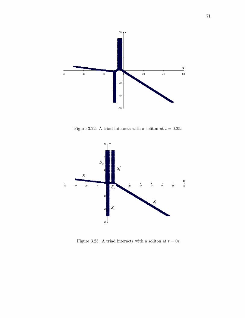
71
Figure 3.22: A triad interacts with a soliton at t = 0.25s
Figure 3.23: A triad interacts with a soliton at t = 0s
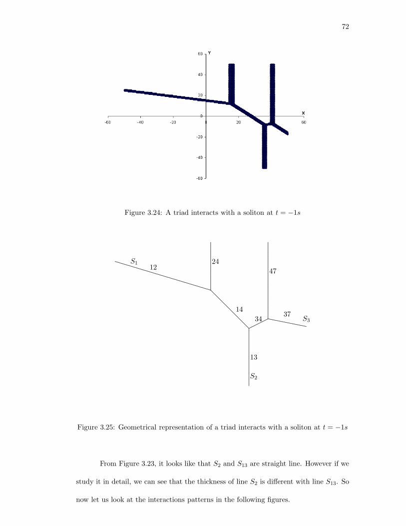
72
Figure 3.24: A triad interacts with a soliton at t = −1s
S3
S2
S112
13
24
1434
47
37
........
........
........
........
........
........
........
........
........
........
........
........
........
........
........
........
........
........
........
........
........
........
........
........
........
........
........
....................................
....................................
..............................................................................................................................................................
........
........
........
........
........
........
........
........
........
........
........
........
........
........
........
........
........
........
........
........
........
........
........
........
........
........
........
........
........
........
........
........
........
........
........
........
..
......................
......................
.......................
......................
.......................
.......................
......................
.......................
.......................
..........
........
........
........
........
........
........
........
........
........
........
........
........
........
........
........
........
........
........
........
........
........
.....
......................................................
.......................................................
......................................................
.......................................................
......................................................
.......................................................
...................................................
Figure 3.25: Geometrical representation of a triad interacts with a soliton at t = −1s
From Figure 3.23, it looks like that S2 and S13 are straight line. However if we
study it in detail, we can see that the thickness of line S2 is different with line S13. So
now let us look at the interactions patterns in the following figures.
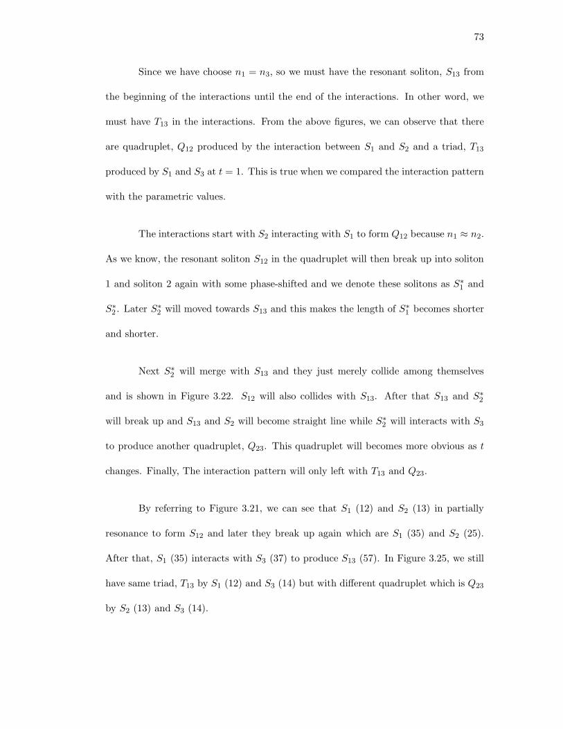
73
Since we have choose n1 = n3, so we must have the resonant soliton, S13 from
the beginning of the interactions until the end of the interactions. In other word, we
must have T13 in the interactions. From the above figures, we can observe that there
are quadruplet, Q12 produced by the interaction between S1 and S2 and a triad, T13
produced by S1 and S3 at t = 1. This is true when we compared the interaction pattern
with the parametric values.
The interactions start with S2 interacting with S1 to form Q12 because n1 ≈ n2.
As we know, the resonant soliton S12 in the quadruplet will then break up into soliton
1 and soliton 2 again with some phase-shifted and we denote these solitons as S∗1 and
S∗2 . Later S∗
2 will moved towards S13 and this makes the length of S∗1 becomes shorter
and shorter.
Next S∗2 will merge with S13 and they just merely collide among themselves
and is shown in Figure 3.22. S12 will also collides with S13. After that S13 and S∗2
will break up and S13 and S2 will become straight line while S∗2 will interacts with S3
to produce another quadruplet, Q23. This quadruplet will becomes more obvious as t
changes. Finally, The interaction pattern will only left with T13 and Q23.
By referring to Figure 3.21, we can see that S1 (12) and S2 (13) in partially
resonance to form S12 and later they break up again which are S1 (35) and S2 (25).
After that, S1 (35) interacts with S3 (37) to produce S13 (57). In Figure 3.25, we still
have same triad, T13 by S1 (12) and S3 (14) but with different quadruplet which is Q23
by S2 (13) and S3 (14).
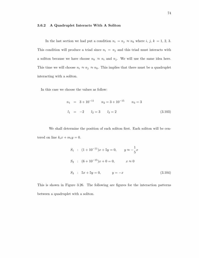
74
3.6.2 A Quadruplet Interacts With A Soliton
In the last section we had put a condition ni = nj ≈ nk where i, j, k = 1, 2, 3.
This condition will produce a triad since ni = nj and this triad must interacts with
a soliton because we have choose nk ≈ ni and nj. We will use the same idea here.
This time we will choose ni ≈ nj ≈ nk. This implies that there must be a quadruplet
interacting with a soliton.
In this case we choose the values as follow:
n1 = 3 + 10−11 n2 = 3 + 10−15 n3 = 3
l1 = −2 l2 = 3 l3 = 2 (3.103)
We shall determine the position of each soliton first. Each soliton will be cen-
tered on line kix + miy = 0.
S1 : (1 + 10−11)x + 5y = 0, y ≈ −15x
S2 : (6 + 10−15)x + 0 = 0, x ≈ 0
S3 : 5x + 5y = 0, y = −x (3.104)
This is shown in Figure 3.26. The following are figures for the interaction patterns
between a quadruplet with a soliton.
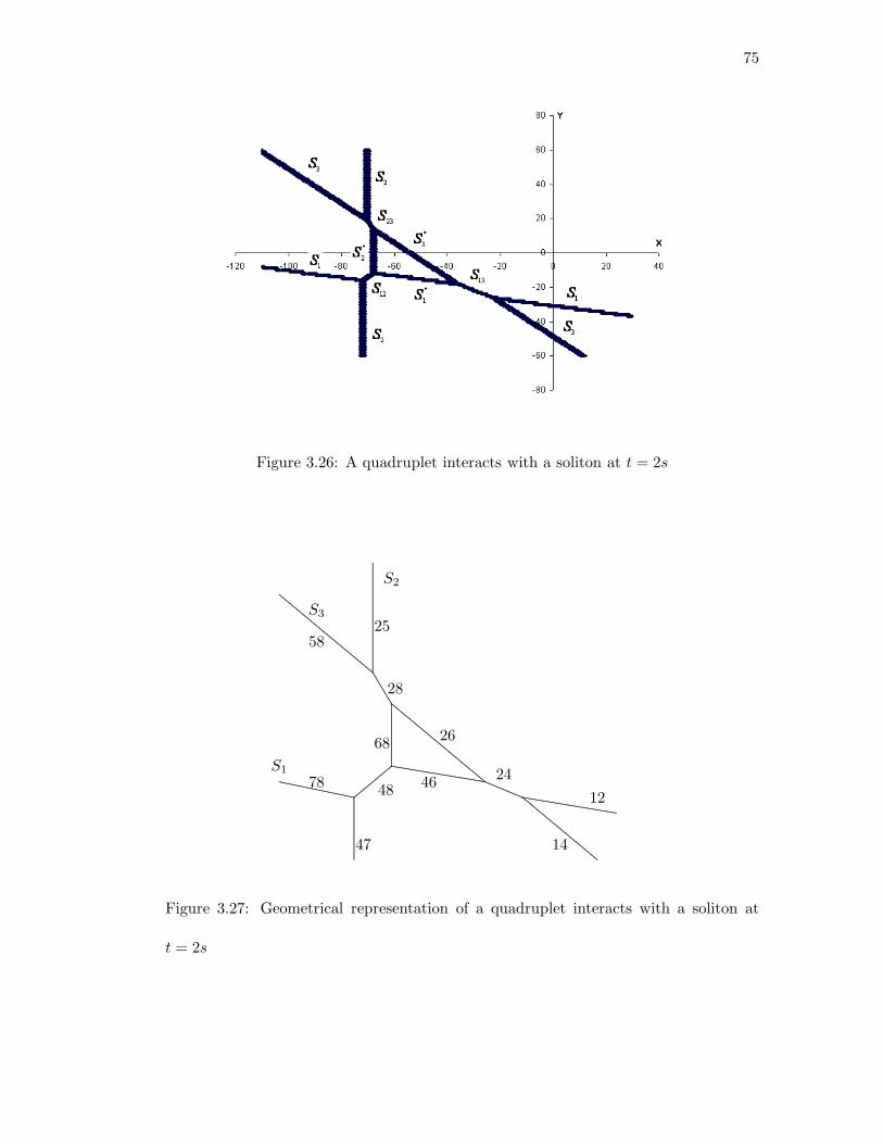
75
Figure 3.26: A quadruplet interacts with a soliton at t = 2s
S3
S2
S1
12
14
24
26
4648
47
78
68
28
5825
..............................................................................................................................................................................................
..................................................................................................................................................................................................................................................................................................................................................................................................................................................................................................................................................................
.........................................................
.............................................................................................................
....................................................................................................................................................................................................................
.................................................................................................................................................................................................................................................................................................................................................................................................................
..........................................................................................................................................................................
Figure 3.27: Geometrical representation of a quadruplet interacts with a soliton at
t = 2s
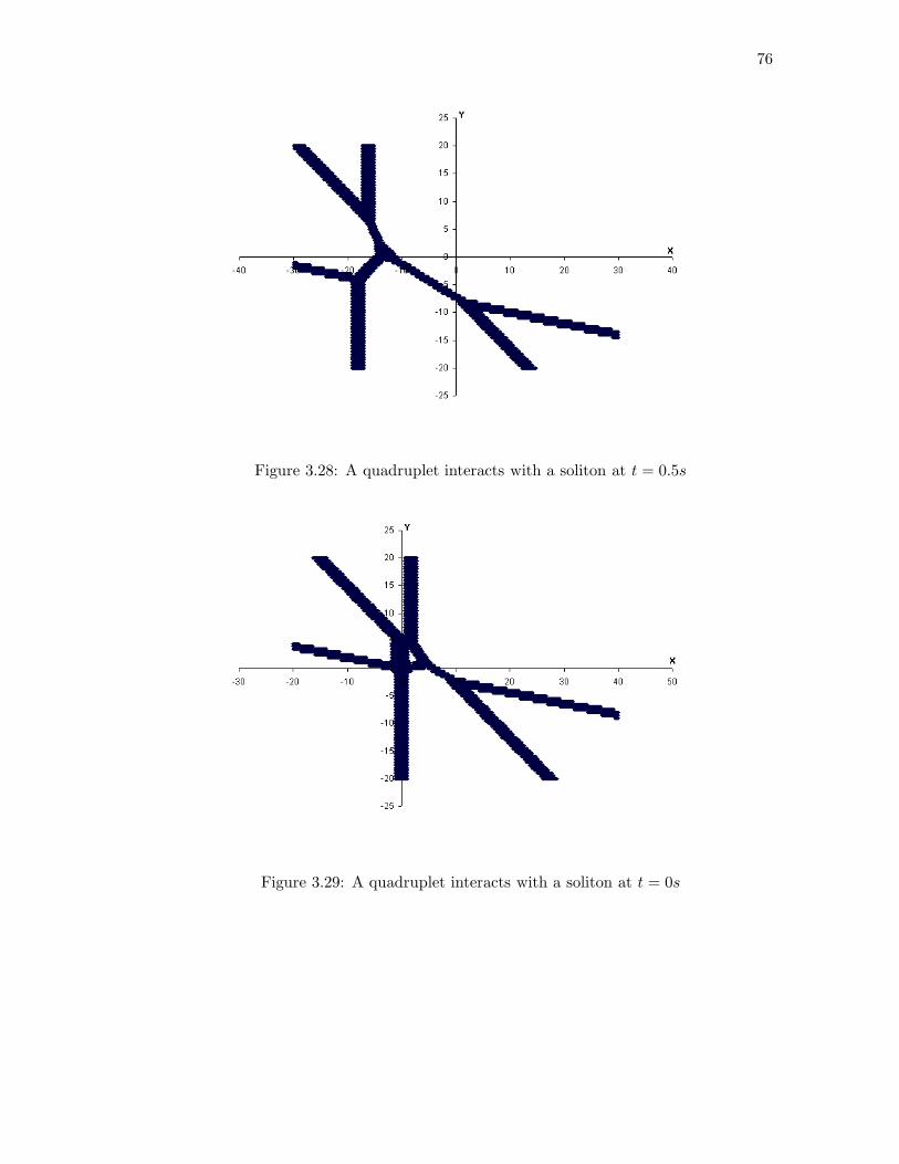
76
Figure 3.28: A quadruplet interacts with a soliton at t = 0.5s
Figure 3.29: A quadruplet interacts with a soliton at t = 0s
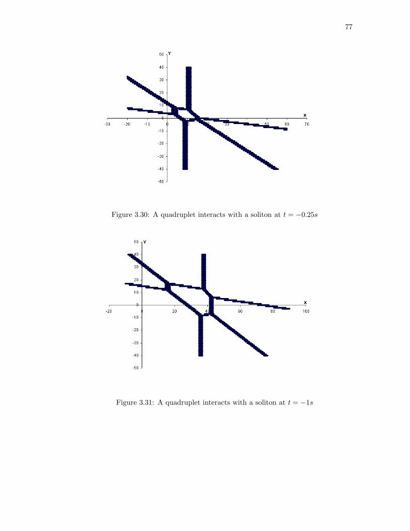
77
Figure 3.30: A quadruplet interacts with a soliton at t = −0.25s
Figure 3.31: A quadruplet interacts with a soliton at t = −1s
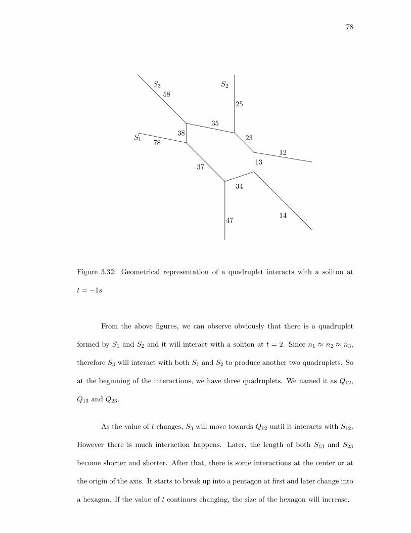
78
S3 S2
S1
12
14
13
23
34
37
47
7838
5825
35
........
........
........
........
........
........
........
........
........
........
........
........
........
........
........
........
........
........
........
........
........
........
........
........
........
........
........
...................................................
.................................................
...................................................................................................................................................................................................................................................................................................................................
........
........
........
........
........
........
........
........
........
.............................................................................................................................................................................................................................
.......................
......................
.......................
.......................
.....................................................................................................................................................................................................................................
................................................................................
................................................................................
.........................................
......................
......................
......................
.......................
.......................
......................
.......................
.......................
......................
.......................
...............
.........................................................................................................................................................
................................................................................
.........................
.............................................................................................................................................................................................................
Figure 3.32: Geometrical representation of a quadruplet interacts with a soliton at
t = −1s
From the above figures, we can observe obviously that there is a quadruplet
formed by S1 and S2 and it will interact with a soliton at t = 2. Since n1 ≈ n2 ≈ n3,
therefore S3 will interact with both S1 and S2 to produce another two quadruplets. So
at the beginning of the interactions, we have three quadruplets. We named it as Q12,
Q13 and Q23.
As the value of t changes, S3 will move towards Q12 until it interacts with S12.
However there is much interaction happens. Later, the length of both S13 and S23
become shorter and shorter. After that, there is some interactions at the center or at
the origin of the axis. It starts to break up into a pentagon at first and later change into
a hexagon. If the value of t continues changing, the size of the hexagon will increase.
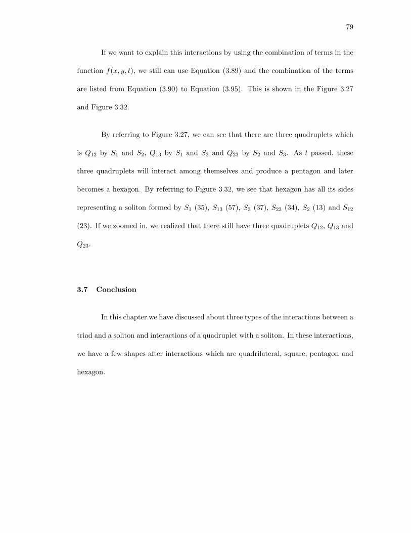
79
If we want to explain this interactions by using the combination of terms in the
function f(x, y, t), we still can use Equation (3.89) and the combination of the terms
are listed from Equation (3.90) to Equation (3.95). This is shown in the Figure 3.27
and Figure 3.32.
By referring to Figure 3.27, we can see that there are three quadruplets which
is Q12 by S1 and S2, Q13 by S1 and S3 and Q23 by S2 and S3. As t passed, these
three quadruplets will interact among themselves and produce a pentagon and later
becomes a hexagon. By referring to Figure 3.32, we see that hexagon has all its sides
representing a soliton formed by S1 (35), S13 (57), S3 (37), S23 (34), S2 (13) and S12
(23). If we zoomed in, we realized that there still have three quadruplets Q12, Q13 and
Q23.
3.7 Conclusion
In this chapter we have discussed about three types of the interactions between a
triad and a soliton and interactions of a quadruplet with a soliton. In these interactions,
we have a few shapes after interactions which are quadrilateral, square, pentagon and
hexagon.
CHAPTER IV
SUMMARY AND CONCLUSIONS
4.1 Introduction
Nonlinearity is a fascinating element of nature whose importance has been ap-
preciated for many years when considering large-amplitude wave motions observed in
various fields ranging from fluids and plasma to solid-state, chemical, biological, and
geological systems. Localized large-amplitude waves called solitons, which propagate
without spreading and have particle-like properties, represent one of the most striking
aspects of nonlinear phenomena.
Today, many scientists see nonlinear science as the most deeply important fron-
tier for fundamental understanding of nature. The soliton concept was firmly estab-
lished after a gestation period of about 150 years. Since then, different kinds of solitons
have been observed experimentally in various real systems, and today, they have cap-
tured the imagination of scientist in most physical discipline. They are widely accepted
as a structural basis for viewing and understanding the dynamics behavior of complex
nonlinear systems.
81
4.2 Summary
In this research we have studied the KP equation and the interactions patterns
produced by solitons interacting. In first chapter, we did some literature review on his-
tory of soliton, properties of soliton, the KdV equation and finally the two dimensional
equation of the KdV equation which is the KP equation.
Furthermore, we have discussed the condition of resonance of the KP equation
in Chapter 2 and we found out that we must have a condition where A12 ≈ 0 so that
resonances occur. Therefore for two-soliton solution, we have three structures which
are triad, quadruplet and cross. The position and direction for every soliton depends
on the values of ni and li. Although we choose and fix the value of ni, we will have
different structures for different value of li since every soliton is centered on the line
kix + miy = 0 or specifically (ni + li)x + (n2i − l2i )y = 0.
From these structures, we can proceed to the interactions of the three KP
solitons. In Chapter 3, we discussed about the interactions patterns between a triad
with a soliton and between a quadruplet and a soliton. We have three versions of the
interactions patterns between triad and a soliton. The difference between these versions
is the sequence for the value of ni with the same value of li. The choice of the sequence
will determine the structure of the triad. Hence this will influence the interactions
patterns. In the interactions of three KP solitons, we can see some patterns produced
after the interactions. For example, we have square, pentagon and hexagon which have
all its sides representing a soliton. On the other hand, we can noticed that the solution
for the interaction between a triad and a soliton can be transformed into Wronskian
determinant.
82
4.3 Suggestion
Since the KP equation has rich mathematical structures, we need to explore
further. We only know little about this equation compared to the KdV equation. Thus
there is a lot of things about the KP equation we can explore. Since the KP equation
is the two dimensional equation for the KdV equation, it is more applicable to the
physical problems. It can be applied into fluid dynamics and other problem in real
world.
The KP equation has been an intensively studied model equation in fluid dynam-
ics. Furthermore, Taniuti and Hasegawa (1991) recently have shown that the nonlinear
development of the magneto sonic waves are governed by the KP equation with the
positive dispersion in some parameter regions (Tajiri and Murakami, 1992). The above
examples show that the KP equation describes many other physical phenomena which
deserves details investigation on it.
Not only the KP equation with the positive dispersion, we also can do some
research on the KP equation with the negative dispersion and forced KP equation.
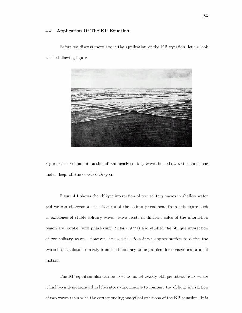
83
4.4 Application Of The KP Equation
Before we discuss more about the application of the KP equation, let us look
at the following figure.
Figure 4.1: Oblique interaction of two nearly solitary waves in shallow water about one
meter deep, off the coast of Oregon.
Figure 4.1 shows the oblique interaction of two solitary waves in shallow water
and we can observed all the features of the soliton phenomena from this figure such
as existence of stable solitary waves, wave crests in different sides of the interaction
region are parallel with phase shift. Miles (1977a) had studied the oblique interaction
of two solitary waves. However, he used the Boussinesq approximation to derive the
two solitons solution directly from the boundary value problem for inviscid irrotational
motion.
The KP equation also can be used to model weakly oblique interactions where
it had been demonstrated in laboratory experiments to compare the oblique interaction
of two waves train with the corresponding analytical solutions of the KP equation. It is
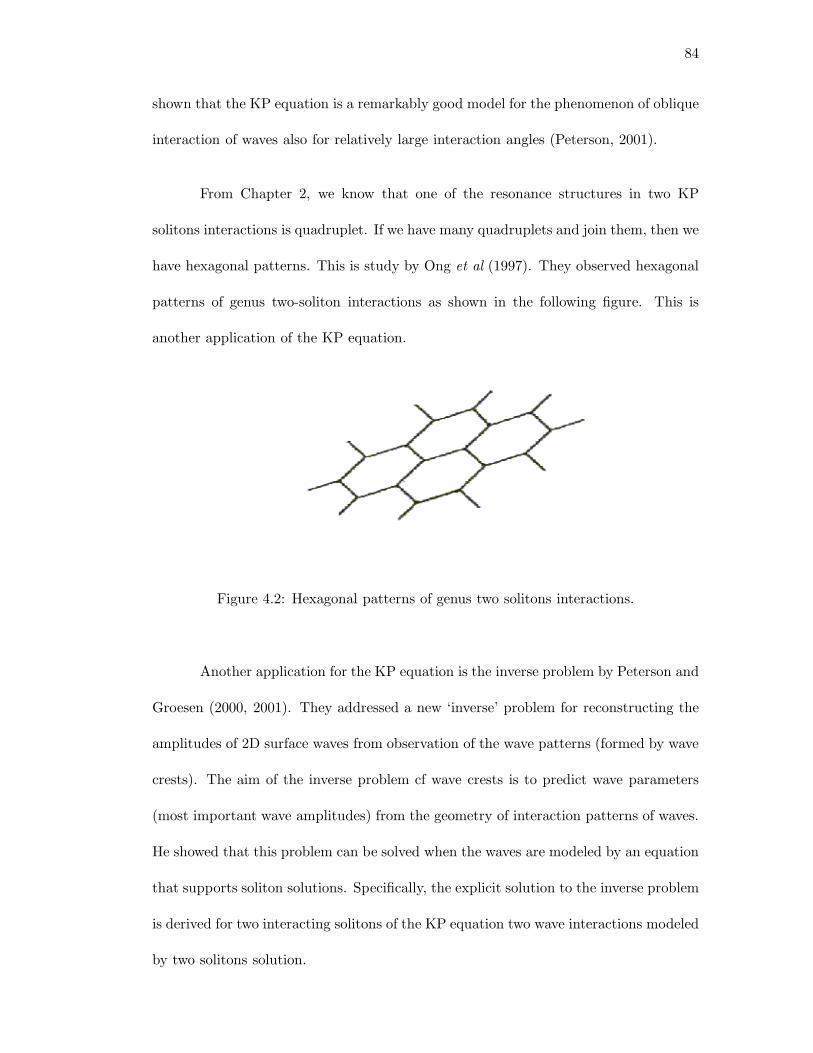
84
shown that the KP equation is a remarkably good model for the phenomenon of oblique
interaction of waves also for relatively large interaction angles (Peterson, 2001).
From Chapter 2, we know that one of the resonance structures in two KP
solitons interactions is quadruplet. If we have many quadruplets and join them, then we
have hexagonal patterns. This is study by Ong et al (1997). They observed hexagonal
patterns of genus two-soliton interactions as shown in the following figure. This is
another application of the KP equation.
Figure 4.2: Hexagonal patterns of genus two solitons interactions.
Another application for the KP equation is the inverse problem by Peterson and
Groesen (2000, 2001). They addressed a new ‘inverse’ problem for reconstructing the
amplitudes of 2D surface waves from observation of the wave patterns (formed by wave
crests). The aim of the inverse problem cf wave crests is to predict wave parameters
(most important wave amplitudes) from the geometry of interaction patterns of waves.
He showed that this problem can be solved when the waves are modeled by an equation
that supports soliton solutions. Specifically, the explicit solution to the inverse problem
is derived for two interacting solitons of the KP equation two wave interactions modeled
by two solitons solution.
85
4.5 Future Research
For future research, we are looking into telecommunication sector, the nano–
technology and also optical solitons. In 1973 Hasegawa and Tappert had proposed that
soliton pulses could be used in optical communications through the balance of non-
linearity and dispersion. They showed that these solitons would propagate according
to the nonlinear Schrodinger equation (NLS), which had been solved by the inverse
scattering method a year earlier by Zakharov and Shabat. At that time there was
no capability to produce the fibers with the proper characteristics for doing this and
the dispersive properties of optical fibers were not known. Also, the system required
a laser which could produce very small wavelengths, which also was unavailable. It
wasn’t until seven years later, when Mollenauer, Stollen and Gordon at AT&T Bell
Laboratories had experimentally demonstrated the propagation of solitons in optical
fibers. The original communications systems employed pulse trains with widths of
about one nanosecond. However, there was still some distortion due to fiber loss. This
was corrected by placing repeaters every several of tens of kilometers. As the width
of the available pulses was decreased, the spacing of the repeaters was increased. In
the mid 1980’s it was proposed that by sending in an additional pump wave along the
fiber, the dispersion of a soliton could be halted through a process known as Raman
scattering. In 1988 Mollenauer and his group had shown that this could be done by
propagating a soliton over 6000 km without the need for repeaters.
Research into the use of solitons as information carriers in optical systems is
still being heavily researched. Soliton pulses are not immune to fiber losses, leading
to pulse broadening. As the pulses broaden, neighboring solitons will overlap and this
overlap is not fully understood. Systems, which allow the propagation of envelope
solitons, operate in the region of negative group velocity dispersion (GVD). However,
86
for positive GVD it has been recently found that a different type of soliton, the so-called
dark soliton, can propagate through optical fibers. The characteristics of these fibers
is currently being investigated. These are just a few of the directions that theoretical
and experimental investigations have taken over the last decade in this rapidly growing
field. It is clear that solitons will play a major role in the next generation of optical
communication systems.
Solitons have been studied in many fields of science; however, the most promis-
ing applications of soliton theory are in the field of optical communications. In such
systems information is encoded into light pulses and transmitted through optical fibers
over large distances. Optical communication systems are the pipe dreams of the future.
Commercial systems have been in operation since 1977. Recently, a transatlantic un-
dersea optical cable has been developed, which is expected to transmit around 40,000
telephone conversations simultaneously. The development of optical fibers, which are
the basis of such systems, has lead to a revolution in communications technology.
Future commercial applications could include adding side branches similar to
those used by the Japanese team to exhaust pipes and other machinery, which might
tame the emitted noise by transforming the loud shock waves into milder solitary waves.
And because the solitary waves can transport energy steadily over a long distance, the
Japanese are exploring potential applications in acoustic compressors, heat engines,
and even heat pumps. Other applications await conceptualization.
Maybe solitons will even find application in the exhaust system of motorcycles,
which would decrease environmental noise pollution.
87
REFERENCES
Anker, D. and Freeman, N. C. (1978). Interpretation of Three-Soliton Interactions
in Terms of Resonant Triads. J. Fluid Mech.. 87: 17-31.
Bhatnagar, P. L. (1979). Nonlinear Waves in One -Dimensional Dispersive Systems.
Oxford: Oxford University Press.
Bullough, R. K. and Caudrey, P. J. (1995). Solitons and the Korteweg-de Vries
Equation: Integrable Systems in 1834-1995. Acta Applicandae Mathematicae.
39: 193-228.
Chow, K. W. (1997). Resonances of Solitons and Dromions. Journal of the Physical
Society of Japan. 66(5): 1282-1287.
Freeman, N. C. (1984). Soliton Solutions of Non-linear Evolution Equations. IMA
Journal of Applied Mathematics. 32: 125-145.
Freeman, N. C. and Nimmo, J. J. C. (1983). Soliton Solutions of the Korteweg de
Vries and the Kadomtsev Petviashvili Equations: the Wronskian Technique.
Proc. R. Soc. Lond.. 389: 319-329.
Gardner, C. S., Greene, J. M., Kruskal, M. D. and Miura, R. M. (1967). Method
for Solving the Korteweg-deVries Equation. Physical Review Letters. 19(19):
1095-1097.
Guo, B. L. (1995). Soliton Theory and Modern Physics. In: Gu, C. H.. Soliton
Theory and Its Application. New York: Springer. 1-5.

88
Kadomtsev, B. B. and Petviashvili, V. I. (1970). On the Stability of Solitary Waves
in Weakly Dispersing Media. Soviet Physics-Doklady. 15(6): 539-541.
Konopelchenko, B. G. (1993). Solitons in Multidimensions: Inverse Spectral Trans-
form Method. Singapore: World Scientific.
Kox, A. J. (1995). Korteweg, de Vries, and Dutch Science at the Turn of the Century.
Acta Applicandae Mathematicae. 39: 91-92.
Kruskal, M. D. and Zabusky, N. J. (1965). Interaction of “Soliton” in a Collisionless
Plasma and the Recurrence of Initial States. Physical Review Letters. 15(6):
240-243.
Miles, J. W. (1977a). Obliquely interacting solitary waves. J. Fluid Mech.. 79:
157-169.
Miles, J. W. (1977b). Resonantly interacting solitary waves. J. Fluid Mech.. 79:
171-179.
Miles, J. W. (1981). The Korteweg-de Vries Equation: A Historical Essay. J. Fluid
Mech.. 106: 131-147.
Miura, R. M. (1978). An Introduction to Solitons and the Inverse Scattering Method
via the Korteweg-deVries Equation. In: Lonngren, K., and Scott A.. Soliton
in Action. United Kingdom: Academic Press. 1-19.
Mukheta bin Isa. Kaedah Penurunan dalam Persamaan Soliton. Seminar Ke-
bangsaan Matematik Gunaan. 3th December 1989-4th December 1989. UTM:
Universiti Teknologi Malaysia. 1989. 1-13.

89
Newell, A. C. (1985). Solitons in Mathematics and Physics. Philadelphia: Society
for Industrial and Applied Mathematics.
Ong, C. T. (1993). Various Aspects in Solitons Interactions. Universiti Teknologi
Malaysia: M.Sci. Thesis.
Ong, C. T. (2002). Development of Numerical Package (FORSO) and Its Applica-
tions on Forced Korteweg-de Vries and Other Nonlinear Evolution Equations.
Universiti Teknologi Malaysia: Ph.D. Thesis.
Ong, C. T., Yuwono, I., Jamaluddin, A. and Jafar. Kadomtsev-Petviashvili (KP)
Wave Identification From Laboratory Observations. RWS’97: Research Work-
shop ‘Aspects of Computational Fluid Dynamics. 9th June 1997-1st August
1997. ITB, Indonesia: Pusat Mathematika, ITB. 1997. 1-14.
Peterson, P. (2001). Multi-Soliton Interactions and the Inverse Problem of Wave
Crests. Tallinn Technical University: Ph.D. Thesis.
Peterson, P. and Groesen, E. V. (2000). A Direct and Inverse Problem for Wave
Crests Modelled by Interactions of Two Solitons. Physica D. 141: 316-332.
Peterson, P. and Groesen, E. V. (2001). Sensitivity of the Inverse Wave Crest Prob-
lem. Wave Motion. 34: 391-399.
Satsuma, J. (1976). N-Soliton Solution of the Two-Dimensional Korteweg-deVries
Equation. Journal of the Physical Society of Japan. 40(1): 286-290.
90
Tajiri, M. and Murakami Y. (1989). Two-Dimensional Multisoliton Solutions: Pe-
riodic Soliton Solution to the Kadomtsev Petviashvili Equation with Positive
Dispersion. Journal of the Physical Society of Japan. 58(9): 3029-3032.
Tajiri, M. and Murakami, Y. (1992). Resonant Interactions between Line Soliton
and Y-Periodic Soliton: Solutions to the Kadomtsev-Petviashvili Equation with
Positive Dispersion. Journal of the Physical Society of Japan. 61(3): 791-805.
Taniuti, T. and Hasegawa, A. (1991). Reductive Perturbation Method for Quasi One-
Dimensional Nonlinear Wave Propagation II: Applications to Magnetosonic
Waves. Wave Motion. 13: 133-146.