Jumpy or Kinky? Regression Discontinuity without theDiscontinuity

Yingying Dong�Department of Economics

University of California Irvine

First draft August 2010, revised July 2012

Abstract

Regression Discontinuity (RD) models identify local treatment effects by associatinga discrete change in the mean outcome with a corresponding discrete change in the prob-ability of treatment at a known threshold of a running variable. This paper shows that it ispossible to identify the RD model treatment effect without a discontinuity. In particular,identi�cation can come from a slope change (a kink) instead of a discrete level change (ajump) in the treatment probability. The intuition is based on L'hopital's rule. The iden-ti�cation results can also be interpreted using instrumental variables models. Estimatorsare proposed that can be applied in the presence or absence of a discontinuity, by exploit-ing either a jump, or a kink, or both. The proposed estimators are applied to investigatethe "retirement-consumption puzzle." In particular, I estimate the impact of retirement onhousehold food consumption by exploiting changes in the retirement probability at 62,the early retirement age in the US.

JEL Codes: C21, C25Keywords: Regression discontinuity, Fuzzy design, Local average treatment effect, Iden-ti�cation, Jump, Kink, Threshold, Retirement, Consumption

�Correspondence: Department of Economics, 3151 Social Science Plaza, University of California Irvine, CA 92697-5100, USA. Email: yyd@uci.edu. http://yingyingdong.com/.

The author would like to thank Arthur Lewbel, Joshua Angrist, James Heckman, Han Hong for very helpful com-ments, and thank Peter Gottschalk and Devlin Hanson for providing the data. Thanks also go to seminar participants atUCI, CSULB and CUHK, as well as conference participants at the SOLE, CEA, and WEAI annual conferences. Anyerrors are my own.

1

1 Introduction

Let T be a binary indicator for some treatment such as participation in a social program or repeating

a grade (grade retention) in school, let Y be some associated outcome of interest such as employment

or academic performance, and let X be a so-called running or forcing variable that affects both T and

Y . For example, X could be age or the income level that affects eligibility for a social program, or

an exam score affecting a grade retention decision. In the standard Regression Discontinuity (RD)

framework, the probability of treatment given by f .x/ D E .T j X D x/ changes discretely at a

threshold point x D c. Under general conditions, this discontinuity or jump in the treatment probabil-

ity f .x/, along with any observed corresponding jump in the mean outcome g .x/ D E .Y j X D x/

at x D c, can be used to recover a local average treatment effect. See, e.g., Hahn, Todd, and van

der Klaauw (2001), Imbens and Lemieux (2008), chapter 6 of Angrist and Pischke (2008), Imbens

and Wooldridge (2009), and Lee and Lemieux (2010). The intuition is that if X and all the other

observed and unobserved covariates determining Y and T are continuous at the threshold c, then in-

dividuals having X just below the threshold will be comparable to those having X just above, and

hence may provide valid counterfactuals. Any mean difference in their outcomes can be attributed to

the difference in their treatment probability.

In this paper I show that the same RD local average treatment effects that are usually identi�ed

by discontinuities can still be identi�ed even if there is no discontinuity or jump, given that there is a

kink, i.e., a slope change in f .x/ at x D c. I also provide estimators that can be used regardless of

whether identi�cation comes from a jump, a kink, or both. This paper focuses on fuzzy design RD

models, since in a sharp design, the treatment probability changes by 1 by di�nition and there is no

slope change at the cutoff. Just as the standard fuzzy design RD estimator is numerically equivalent to

an instrumental variable (IV) estimator (Hahn, Todd, van der Klaauw, 2001), I show that the proposed

estimators are numerically equivalent to IV estimators.

One may wonder where the slope change comes from in real applications. Most existing applica-

tions of fuzzy design RD models already acknowledge slope changes in the treatment probability by

allowing the slopes to be different on both sides of the cutoff. However, they don't utilize the slope

change for identi�cation. For a standard fuzzy design RD model, the size of the discontinuity in the

treatment probability can be any value between zero and one (not including one). In any particular

empirical application, how large the discontinuity is depends on the incentive generated by the partic-

2

ular policy rule. One would not be able to tell beforehand the size of the discontinuity even if knowing

the institutions. Estimating the exact size of the discontinuity showing how strong the policy incentive

is might be an interesting empirical issue itself. It is possible that when the incentive is weak enough,

one won't see a signi�cant jump at the cutoff. This paper's approaches can be applied to situations

like this when the standard RD identi�cation fails.

Assume that the treatment probability changes smoothly with the running variable in the absence

of the policy rule (e.g. the retirement rate changes smoothly with age without the pension rule). The

discrete change in slope at the cutoff can occur if the policy bene�ts or incentives depend on how far

one is from the threshold, or an administrator's discretion or incentive to assign treatment depends

on one's distance from the threshold. In other words, the policy incentive is interacted with the

distance from the cutoff. In these cases, the added probability of treatment associated with crossing a

threshold may rise as one gets further away from the threshold. Treatment effects based on standard

RD estimators would either be weakly identi�ed, if the jump is small, or unidenti�ed if the jump is

zero, regardless of how much the slope changes. In contrast, the estimators proposed in this paper

make use of any changes in either the intercept or the slope of the treatment probability at the point

x D c.

Jacob and Lefgren (2004) examine the effect of remedial education programs, including grade

retention, on later academic performance, where the treatment, grade retention, is incurred by failing

summer school tests. They note that "the probability of retention does not drop sharply (discontinu-

ously) at the exact point of the cutoff , ...it rapidly decreases over a narrow range of values just below

the cutoff." Indeed, their Figure 7 (reproduced in Figure 1 here) clearly shows a dramatic slope change

and a zero discontinuity gap in the retention probability at the cutoff (normalized to zero). In this case,

the standard RD estimation based on a discrete change in the treatment probability is not applicable,

whereas the estimators proposed in this paper may still apply. Note that the result in this �gure is not

an artifact of the discretization of test scores.1;2

1Test scores in this case are grade equivalents (GEs), and they are typically reported up to the tenths place. Another�gure of the paper, Figure 4 shows the probability of attending summer school conditioning on the same measures of testscore. Clearly the probability of attending summer school has a much sharper change at the cutoff than the probabilityof repeating a grade. The standard RD model applies, and in fact the authors use the standard RD model to estimate theeffect of attending summer school. It can be shown that discretization or rounding error would bias upward, rather thandownward, the estimated discontinuity in the probability of grade retention (Dong, 2012).

2This lack of a jump in the retention rate at the cutoff score can be further justi�ed on institutional grounds. Actualretention policies vary across school districts in the US. At least in some schools, the decision of holding students backis made in part based on whether their standard test scores fall below a cutoff. However, given that repeating a grade is acostly decision, the cutoff is usually used only as a reference, and schools take into account how far students fall below

3

Figure 1: Retention Rate and Reading Test Scores Relative to the Cutoff

In some potential applications of RD models, there is debate about whether the probability of

treatment actually jumps at a threshold. When a discrete change is small, it could be indistinguishable

from a kink. An example is Figure 2, which reproduces Figure 4 from Card, Dobkin, and Maestas

(2008), showing the employment rates in the US by age. It is dif�cult to determine whether a small

jump appears at age 65, the eligibility age for full social security bene�ts, but there is an obvious

difference in slopes above and below this threshold. The estimators proposed in this paper might then

be used to identify the impact of employment on outcomes like heath conditions among the close to

retirement age people, based just on the knowledge that the propensity to work has either a jump or a

kink at 65.3

For simplicity, this paper will mostly not deal with covariates other than the running variable

X in the analysis. The standard RD argument applies that covariates are generally not needed for

consistency in estimating the average (unconditional) treatment effect, though they may be useful for

the cutoff. Those students who are right at the cutoff between passing and failing are less likely to be held back, whilethose who score further below the cutoff are more likely to repeat a grade. This is precisely what could cause a kink ratherthan a jump, as is seen in Figure 1 here.

3Since age (in quarters) is used as a running variable, individuals are not likely to manipulate their age to sort near thecutoff, and so the observed kink should not be caused by endogenous sorting.

4

Figure 2: Employment Rates by Age and Demographic Group (1992�2003 NHIS)

ef�ciency or for testing the validity of RD assumptions. However, if desired, additional covariates Z

could be included in the analysis by letting all the assumptions hold conditional upon the values Z

may take on.4 In applications, one could either partial out these covariates prior to analysis, or include

them in the models as additional regressors.

I apply the proposed estimators to estimate the impact of retirement on household food consump-

tion at 62, the early retirement age in the US. Graph analyses show that food consumption and retire-

ment may have a jump and/or a kink at 62, so estimators based on either a jump, or a kink, or both

are performed. It's shown that using either one or both sharp changes in the retirement probability at

62 yields very similar estimates and that the results are robust to different estimation windows (band-

widths) and weightings (kernel functions). Food consumption is estimated to drop by about 15% to

23% when household heads retire at 62.

The rest of the paper is organized as follows. Section 2 reviews the related literature. Section 3

provides the main identi�cation results. Section 4 gives an instrumental variables interpretation of the

identi�cation results. Section 5 discusses some extensions, including possible identi�cation based on

higher order derivatives. Section 6 provides associated estimators. Section 7 presents an empirical4Conditional on Z is necessary if treatment effects vary across covariate values and if one is interested in estimating

conditional treatment effects.

5

application, and Section 8 concludes.

2 Literature Review

This section reviews two strands of literature, the standard RD literature and the recent regression

kink design literature. This paper is directly built upon the standard RD literature, which is originated

in Thistlethwaite and Campbell (1960). Recent comprehensive reviews of the RD literature include

Imbens and Lemieux (2008), van der Klaauw (2008), and Lee and Lemieux (2010).

In a seminal paper, Hahn, Todd, and van der Klaauw (2001) formally show the RD identi�cation

in the treatment effect framework and provide assumptions required to identify causal effects. They

also propose local linear estimators for nonparametric estimation of the RD treatment effect. Porter

(2003) proposes alternative nonparametric estimators and discusses optimal convergence rates. Lee

(2008) establishes weak behavioral conditions under which causal inferences from RD analysis can

be credible. In particular, Lee (2008) shows that when agents have only imprecise control over the

running variable and hence the running variable, along with other covariates, is continuous at the

cutoff (due to the random component), RD analysis can still deliver valid inferences. Lee suggests

to test this assumption by examining whether baseline covariates are continuous at the threshold of

the running variable. McCrary (2008) develops a formal density test to test the manipulation of

the running variable. Lee and Card (2008) consider the case when the running variable is discrete.

They interpret deviations of the chosen approximating regression function from the true regression

function as random speci�cation errors and discuss the impact of this on inference. In particular, they

recommend clustering the standard error at the cell level and show how to do more ef�cient estimation

in this case. Imbens and Kalyanaraman (2012) discuss the optimal bandwidth choice for RD models.

A recent literature considers a regression kink design. Important work in this literature include

Nielsen, Sorensen, and Taber (2009), and Card, Lee, and Pei (2009). Nielsen, Sorensen, and Taber

(2009) �rst introduce Regression kink design (RKD) in their study of �nancial aid effect on college

enrollment. They propose an estimand for their RKD, which takes the form of the ratio of the slope

change or kink in the conditional mean of outcome and the kink (the subsidy rate change) in the

magnitude of a continuous treatment (the amount of subsidy) as a function of the running variable

(family income). Other empirical studies that use kinks to identify effects of continuous endogenous

regressors include Guryan (2003) and Simonsen et al. (2009).

6

Related to RKD, the paper by Card, Lee, and Pei (2009) considers nonparametric identi�cation

of the average marginal effect of a continuous endogenous treatment variable in a generalized non-

separable model, where the treatment of interest is a known, deterministic but kinked function of an

observed continuous assignment variable. They also characterize a broad class of models for which a

RKD provides valid inferences regarding the underlying marginal effects. Under suitable conditions

they show that the RKD estimand identi�es the "treatment on the treated" parameter.

The models in Nielsen, Sorensen, and Taber (2009) and Card, Lee, and Pei (2009) can be taken

as sharp designs in the sense that everyone is a complier and obeys the same treatment assignment

rule, but the treatment intensity varies. In particular, the treatment is continuous and is assumed to

be a known deterministic function of the running variable. The fundamental identi�cation problem

is then to separate the effect of the potentially endogenous running variable from that of treatment

in a general nonparametric model, because the latter is completely determined by the former. The

identi�cation is based on the magnitude of the treatment as a kinked function of the running variable.

The goal of this paper, however, is to identify the same treatment effect parameter of interest

as in the standard fuzzy design RD models, but under more general conditions. In particular, this

paper considers RD models where the treatment is binary, and the functional form for the treatment

is unknown. As in the standard RD literature, the estimated effect is a local average effect local at the

threshold of the running variable. The identi�cation is based on a kink instead of or in addition to a

jump.

The purely kink-based estimand (Theorem 1) in this paper super�cially resembles the RKD esti-

mand as in Nielsen, Sorensen, and Taber (2009) and Card, Lee, and Pei (2009). A key difference is

that the RKD estimand depends on the derivative of the treatment variable, which would be infeasible

when treatment is binary, while the estimand here depends on the derivative of the expected value of

a binary treatment, i.e., the treatment probability. This paper also discusses generalizations that work

regardless of whether the treatment probability has a jump, a kink, or both. In addition, this paper

shows the identi�cation results (and the proposed estimators) can be intuitively interpreted using IV

models. This extends the known result that the standard RD estimator is numerically equivalent to an

IV estimator although the IV validity assumption does not hold, as noted by Hahn, Todd, and van der

Klaauw (2001).

7

3 RD Treatment Effects without A Discontinuity

I will use Rubin's (1974) potential outcome notation. Let Y .1/ and Y .0/ denote an individual's

potential outcomes from being treated or not, respectively. The observed outcome can then be written

as Y D Y .1/ T C Y .0/ .1� T /. As in the introduction, de�ne g .x/ D E .Y j X D x/ and f .x/ D

E .T j X D x/, so g .x/ and f .x/ are the expected outcome and expected probability of treatment

when the running or forcing variable is X D x . In the standard RD model one would expect both

f .x/ and g .x/ to have a jump (discontinuity) at the �xed threshold x D c.

Let T � be a dummy for crossing the threshold c, i.e., T � D I .X � c/, so T � is one for individuals

who have X above the threshold and zero otherwise. De�ne the potential treatment status variables

T .0/ and T .1/, i.e., what an individual's treatment status would be if T � D 0 or T � D 1. A complier

can then be de�ned as an individual who has T .0/ < T .1/, so a complier is an individual who takes

up treatment if and only if he crosses the threshold. Let D� be a binary indicator for compliers, i.e.,

D� D 1 if an individual is a complier and 0 otherwise. E .D� j X D x/ then equals the compliance

rate among all individuals having X D x for x in a neighborhood of c. We do not observe D� and

so do not know who are compliers. Assumption A1 below and Lemma 1 later make it clear that

by conditioning on compliers, one does not have to impose additional conditions like the conditional

mean independence or alternative assumptions as imposed by Hahn, Todd, and van der Klaauw (2001,

Theorem 2) for identi�cation of the RD model treatment effect in a general setup.5

The standard RD model requires E .D� j X D c/ 6D 0, which would result in f .x/ having a

discontinuity at c. The sharp design RD model is the special case where E .D� j X D c/ D 1 so

everyone is a complier.

ASSUMPTION A1: Assume that for each unit (individual) i we observe Yi , Ti , and X i . The

threshold c is a known constant. The conditional means E.Y .t/ j X D x; D� D 1/ for t D 0; 1,

E.Y j X D x; D� D 0/, and E.T j X D x; D� D 0/, as well as E.D� j X D x/, are continuously

differentiable for all x in a neighborhood of x D c.

For ease of notation I will drop the i subscript when referring to the random variables Y , T , and

X .5Battistin et al. (2009) similarly derive the treatment effect estimator without imposing the conditional mean indepen-

dence assumption for their one-sided fuzzy design RD model. They do so by conditioning on treatment equal to one rightabove the cutoff (equation (16) in their Web Appendix), which given the one-sided fuzziness of their RD model is thesame as conditioning on compliers.

8

Assumption A1 says that for compliers the conditional mean potential outcomes E.Y .t/ j X D

x; D� D 1/ for t D 0; 1 are smooth, for noncompliers the conditional mean outcome E.Y j X D

x; D� D 0/ and treatment probability E.T j X D x; D� D 0/ are smooth, and the treatment proba-

bility change or the compliance rate E.D� j X D x/ is also smooth. All this required smoothness is

in the sense of continuous differentiability. Intuitively, these assumptions rule out individuals' sort-

ing behavior, i.e., it is assumed that individuals can not precisely manipulate the running variable

to be just above or below the threshold and hence take or avoid the treatment (more discussion on

this can be found in Lee 2008). These assumptions also rule out de�ers, i.e., individuals who have

T D 1� T � for all x in the neighborhood of c, guaranteeing that any jumps or kinks in the outcome

or the treatment probability are due only to compliers. Below provides further discussion.

Assumption A1 differs from the standard RD assumptions in requiring more smoothness. For

example, standard RD models require only continuity of the conditional mean potential outcomes for

identi�cation rather than continuous differentiability. This paper requires additional smoothness to

rule out not only jumps but also kinks (formally de�ned below) caused by factors other than changes

in the treatment probability at the threshold x D c. In practice, estimators of standard RD models

generally impose at least as much smoothness as Assumption A1. For example, standard asymptotic

properties of kernel or local linear regressions require continuous differentiability. Similar continuous

differentiability of conditional potential outcomes in the running variable X is also used by Dong and

Lewbel (2010) to identify the treatment effect change given a marginal change in the threshold.

Assumption A1 imposes smoothness on the conditional mean potential outcomes conditioning on

compliers (D� D 1).6 One could instead impose smoothness without conditioning on D� D 1 by

having either a constant treatment effect or a local conditional independence of treatment assumption,

i.e., having potential outcomes conditional on X D x be independent of treatment in a neighborhood

of x D c, as in Hahn, Todd, and van der Klaauw (2001).

For noncompliers (D� D 0), Assumption A1 requires their conditional mean outcome E.Y j

X D x; D� D 0/ to be smooth at the cutoff, so the observed outcome difference when crossing the

threshold are from compliers. By assuming smoothness of E.T j X D x; D� D 0/, Assumption A1

rules out a positive probability of de�ers.6Intuitively, the smoothness of potential outcomes along with the de�nition of compliers means that among compliers

those just below the cutoff would provide valid counterfactuals for those just above. Note that this still allows for self-selection into the group of compliers.

9

One way to interpret the smoothness of E.Y j X D x; D� D 0/ is to assume that there exists

a small neighborhood of c where noncompliers consist of always-takers and/or never-takers. Then a

suf�cient condition for the smoothness of the conditional mean outcome for noncompliers would be

continuous differentiability of their conditional mean potential outcomes, i.e., E.Y .t/ j X D x; D� D

0/ for t D 0; 1. This is due to the fact that for both always-takers and never-takers, treatment status

does not change and hence is smooth when crossing the threshold, i.e., treatment is always one for

always-takers, and zero for never-takers, and that E.T j X D x; D� D 0/ and E.D� j X D x/ are

assumed to be smooth at the cutoff.

Smoothness of E.T j X D x; D� D 0/, i.e., no de�ers, means that E.D� j X D x/ equals the

change in the treatment probability at X D x . The smoothness of E.D� j X D x/ then guarantees that

its ordinary derivative exists and that its one-sided derivatives equal the ordinary derivative at x D c.

Results in this paper require one-sided limits and one-sided derivatives. For any function h .x/, de-

�ne (when they exist) hC .x/ and h� .x/ as the right-sided and left-sided limits, and de�ne h0C .x/ and

h0� .x/ as the right-sided and left-sided derivatives, respectively. Also let h0 .x/ D @h .x/ =@x . A stan-

dard result is that if h .x/ is differentiable, then h0C .x/, h0� .x/, and h0 .x/ exist and h0C .x/ D h0� .x/ D

h0 .x/. With these notations, a discontinuity at x D c means fC .c/ � f� .c/ 6D 0, and the treatment

effect estimated by standard RD models can be written as .gC.c/� g�.c// = . fC.c/� f�.c//.

LEMMA 1: If Assumption A1 holds then

gC.c/� g�.c/ D � .c/ E�D� j X D c

�(1)

and

fC.c/� f�.c/ D E�D� j X D c

�, (2)

where

� .c/ D E�Y .1/� Y .0/ j X D c; D� D 1

�. (3)

Proofs are in the Appendix. Lemma 1 shows that Assumption A1 suf�ces to reproduce the stan-

dard result in the RD literature. In particular, it follows immediately from Lemma 1 that if there is a

10

discontinuity, meaning that fC.c/� f�.c/ 6D 0, then

� .c/ DgC.c/� g�.c/fC.c/� f�.c/

. (4)

That is, the standard RD treatment effect estimator estimates � .c/ D E.Y .1/� Y .0/ j X D c;

D� D 1/, the average treatment effect for the compliers (D� D 1) at the threshold c, as discussed

in, e.g., Hahn, Todd, and van der Klaauw (2001) and Imbens and Lemieux (2008). Under some

conditions Assumption A1 can be extended to allow for de�ers.7

I now consider identifying this RD model treatment effect under alternative assumptions. In par-

ticular, I consider: What if there is no jump in the treatment probability? Can we still identify the RD

local average treatment effect when there is no discontinuity? Formally de�ne a jump and a kink as

follows.

DEFINITION: At the point x , a jump in the function f .x/ (or simply a jump) is de�ned as

fC .x/� f� .x/ 6D 0 and a kink in the function f .x/ (or simply a kink) is de�ned as f 0C .x/� f 0� .x/ 6D

0.

THEOREM 1: Let Assumption A1 hold. Assume there is a kink but no jump at x D c. Then

�.c/ Dg0C .c/� g0� .c/f 0C .c/� f 0� .c/

: (5)

Theorem 1 shows that the RD treatment effect is identi�ed without a discontinuity, and an esti-

mator can be easily constructed based on Theorem 1. Note that Assumption A1 suf�ces to guarantee

that the one-sided derivatives g0C .x/, g0� .x/, f 0C .x/, and f 0� .x/ exist at x D c. Theorem 1 says that

if there is no jump in f .x/, then the treatment effect will equal the ratio of the kinks in g.x/ and

f .x/ at x D c instead of the ratio of the jumps. The reasoning is that if f .x/ does not have a jump,

then both the denominator and the numerator of the standard RD estimator given by equation (4) will7For example if one is willing to assume locally constant treatment effects, then Assumption A1 could be easily

extended to allow for de�ers as follows. Let d� be a binary indicator for de�ers, so d� D 1 for individuals who haveT .1/ < T .0/. Then in addition to assuming smoothness of E.Y .t/ j X D x; D� D 1/, one also needs to similarly assumesmoothness of E.Y .t/ j X D x; d� D 1/. Furthermore, one needs to replace E.Y j X D x; D� D 0/ and E.T j X Dx; D� D 0/ in Assumption A1 with E.Y j X D x; D� D d� D 0/ and E.T j X D x; D� D d� D 0/, respectively, andreplace E.D� j X D x/ with E.D� � d� j X D x/. In this case, Lemma 1 would hold by replacing equation (2) withfC.c/� f�.c/ D E.D� � d� j X D c/ and replacing equation (3) with � .c/ D E .Y .1/� Y .0/ j X D c/.

11

equal zero as x goes to c. Intuitively in this case, by L'hopital's rule, that ratio will equal the ratio

of derivatives of the numerator and denominator, given that these derivatives exist. A formal proof is

provided in the Appendix.

Theorem 1 requires that the slope of the treatment probability changes at the threshold, which pro-

vides identi�cation. So unlike in the standard RD model where the treatment effect �.c/ is identi�ed

off a jump in the treatment probability, here �.c/ is identi�ed off a kink.

In a standard RD model individuals just below the cutoff and those just above are comparable

and so their mean outcome difference can be attributed to the treatment probability change. Here,

individuals just below the kink point and those just above are also comparable, so one can use the

slope change of their mean outcome and the associated slope change of their treatment probability to

identify the local average treatment effect at the cutoff.

Just as jumps in the density of X or conditional means of other baseline covariates at the threshold

would cast doubt on the validity of the smoothness assumption in standard RD models, unusual jumps

and kinks in the density of X or conditional means of other baseline covariates at the threshold would

indicate individual sorting or manipulation of the running variable, and hence would cast doubt on the

validity of the smoothness assumption in A1, and hence in this case, the identi�ed �.c/ in Theorem

1 would not be interpretable purely as a causal effect. To address this concern, one can easily extend

the standard RD validity tests, e.g., tests on the smoothness of the density of the running variable and

the smoothness of the conditional means of covariates, to this paper's case.

A formal test of continuity of density can be found in McCrary (2008). More informally, one

could draw a histogram of X based on a �xed number of bins on each side of the cutoff. The overall

shape of the distribution can provide a sense whether there is an unusual jump or kink in the density of

X at the cutoff. Alternatively, on each side of the cutoff one could do a linear regression of the number

of observations in each bin on the mid-point value of each bin and examine if there is a signi�cant

intercept or slope change.

For other base-line covariates, analogous to the test suggested by Lee (2008) and Lee and Lemieux

(2010), one could do a parallel RD analysis by replacing the outcome variable Y with these covariates

and examine the signi�cance of the coef�cients on T , for which the equation includes both a jump

T � and a kink .X � c/T �. Finding a signi�cant effect of treatment on these pre-determined baseline

covariates would suggest unusual jumps or kinks of these covariates at the cutoff. Alternatively, one

could do local linear regressions of these covariates at each side of the threshold to examine if there

12

is an intercept or slope change in those variables at the threshold.8

Combining Lemma 1 with Theorem 1 gives the following Corollary.

ASSUMPTION A2: Assume there is either a jump or a kink (or both) at x D c.

COROLLARY 1: Let Assumptions A1 and A2 hold. Assume that the one-sided limits and one-

sided derivatives of f .x/ and g.x/ at x D c are identi�ed from the data. Then �.c/ is identi�ed.

The econometrician does not need to know if there is a jump, a kink, or both. As long as either one

or both are present, Corollary 1 says that the treatment effect can be identi�ed. Given the identi�cation

in Corollary 1, the following Theorem 2 provides a way to estimate the treatment effect. In each of

the remaining theorems and corollaries, estimators are obtained by replacing functions g and f with

corresponding estimatesbg and bf .THEOREM 2: Assume A1 and A2 hold. Given any sequence of nonzero weights wn such that

limn!1wn D 0, then

�.c/ DgC .c/� g� .c/C wn

�g0C .c/� g0� .c/

�fC .c/� f� .c/C wn

�f 0C .c/� f 0� .c/

� . (6)

Theorem 2 uses a weight wn to combine both the standard RD estimator (4) and the new kink

based estimator (5). When there is no jump, i.e., fC.c/� f�.c/ D 0, then equation (6) will reduce to

equation (5). Similarly when there is no kink, i.e., f 0C .c/� f 0� .c/ D 0, then equation (6) will reduce

to equation (4). In practice, if one is sure that there is no jump or no kink, then it will generally be

preferable to base estimation directly on equation (4) or equation (5) rather than equation (6), because

in that case equation (6) will entail estimation of the terms that are known to equal zero.

When one is unsure whether an observed break at X D c is a jump or a kink, or both, The-

orem 2 can be applied to construct consistent estimators for �.c/, which might be appealing em-

pirically. Theorem 2 requires the weight to go to zero as the sample size goes to in�nity, so as-

ymptotically it sets �.c/ equal to the standard RD estimator as long as there is a jump, regardless

whether there is a kink. The following Corollary 2 makes it clear that the kink based estimator

g0C .c/ � g0� .c/ =�f 0C .c/� f 0� .c/

�does not converge to the same local average treatment effect as

8The latter, when using a uniform kernel, visually corresponds to using a �xed number of bins on each side of X D cand graphing the mean value of each covariate in each bin against the mid-point of those bins.

13

the jump based estimator when there is a jump, unless � 0.c/ D 0 holds. In Section 4, I show that the

weights in the local 2SLS estimator, a special case of the proposed estimator here, have this property.

Theorem 2 justi�es on a formal ground that local 2SLS estimators utilizing both the jump and kink as

IV's are valid estimators when one is not sure whether there is a jump, a kink or both.

All the results so far place no restriction on � 0.c/. The following Corollary provides a weighted

estimator that does not require the weight to have the feature as in Theorem 2. Essentially any weights

can be used to combine identi�cation from the jump and that from the kink. Corollary 2 instead

requires � 0.c/ D 0. Results from Corollary 2 can in fact be used to test this condition. Compared with

Theorem 2, the advantage of Corollary 2 is that when this condition holds, Corollary 2 can exploit

information from both the jump and the kink to identify �.c/ instead of just the jump asymptotically

as Theorem 2.

COROLLARY 2: Assume A1 and A2. When both a jump and a kink exist, assume � 0.c/ D 0.

Then

�.c/ DgC .c/� g� .c/C w

�g0C .c/� g0� .c/

�fC .c/� f� .c/C w

�f 0C .c/� f 0� .c/

� (7)

for any w 6D � . fC .c/� f� .c// =�f 0C .c/� f 0� .c/

�.

� 0.c/ D 0 means that the treatment effect does not vary linearly with the running variable X , as

in the case where the treatment effect is locally constant. The proof of Corollary 2 shows that given

� 0.c/ D 0, both gC .c/ � g� .c/ = . fC .c/� f� .c// and g0C .c/ � g0� .c/ =�f 0C .c/� f 0� .c/

�can be

valid estimands for the treatment effect �.c/, i.e., they converge to the same limiting value, so they

can be combined using any valid weights. When the treatment effect varies linearly with X , however,

the kink based estimator would not converge to same the local average treatment effect as the jump

based estimator does.

Note that � 0.c/ D 0 is a strictly weaker condition than assuming a locally constant treatment

effect, because the latter would imply that all derivatives of �.c/ were zero, not just the �rst derivative

� 0.c/. I will discuss the interpretation of this restriction in more detail in Section 4, and provide an

extension to Corollary 2 in Section 5. This extension will permit � 0.c/ to be non-zero.

Except for providing a way to estimate the standard RD treatment effect regardless one has a jump,

a kink, or both, Corollary 2 can also be used is to construct a simple test regarding locally constant

14

treatment effects when the treatment probability has both a jump and a kink. De�ne � 1 and � 2 by

� 1 D .gC .c/� g� .c// = . fC .c/� f� .c//

� 2 D�g0C .c/� g

0� .c/

�=�f 0C .c/� f 0� .c/

�.

If the treatment effect is locally constant, then � 0.c/ D 0, and by Corollary 2 one will have both

� 1 D � 2 D �.c/, so one could test � 0.c/ D 0 by testing whether the difference between the two

corresponding estimatesb� 1 andb� 2 is signi�cant. Failing this test indicates that the treatment effect isnot locally constant. For parametric RD models, this amounts to a simple t test with the test statistic

.b� 1 �b� 2/ =� .b�1�b�2/, where the denominator is the standard error of the differenceb� 1 �b� 2.The weightw could be chosen to maximize ef�ciency, i.e., choosing the value ofw that minimizes

the estimated standard error of the corresponding estimate of �.c/. The following Section 4 provides a

two stage least squares estimator (2SLS) that uses weights based on a measure of the relative strength

of the two possible sources of identi�cation, the jump and kink.9 For any �nite sample, the weights

are non-zero, but asymptotically, the strength of the kink goes to zero as the sample size goes to

in�nity and hence the bandwidth shrinks to zero.

Estimators based on the above theorems and corollaries are discussed in greater detail later. For

now observe that one could directly construct nonparametric estimators of gC .c/ and g0C .c/ as the

intercept and slope of a local linear regression of Y on X � c just using data having X > c. Doingthe same with data having X < c will give estimators of g� .c/ and g0� .c/. Replacing Y with T in

the local linear regressions above and below the threshold will give estimates of fC .c/, f 0C .c/, f� .c/

and f 0� .c/. These could then be substituted into equations (6) or (7) to obtain consistent estimates of

�.c/.

4 Instrumental Variables Interpretation

This section provides an instrumental variables interpretation for the identi�cation results of the pre-

vious section. This extends the known result by Hahn, Todd and van der Klaauw (2001) that the

standard fuzzy design RD estimator based on discontinuities is numerically equivalent to an IV esti-9The result is not surprising. It is in fact a generic feature of 2SLS that when there exit more than one instrumental

variables, 2SLS uses ef�cient weights in combining these instrumental variables (see, e.g., Davidson and MacKinnon,1993, and Chapter 4 of Angrist and Pischke, 2008).

15

mator. I show that when there is either a jump, or a kink, or both, the RD treatment effect estimators

are numerically equivalent to IV estimators. I will also show how instrumental variable methods can

be used to construct simple estimators based on these results.

Suppose that for c � " � X � c C " for some small positive ", one has the outcome model

Y D � C �.X � c/C �T C e; (8)

where �, �, and � are coef�cients, and the error e may be correlated with the treatment indicator T .

In general, e might also be correlated with X and hence T � for strictly positive ". Hahn, Todd, and

van der Klaauw (2001) show that the standard fuzzy design RD estimator given by equation (4) is

numerically equivalent to the IV estimator of � in equation (8), using .X � c/ and T � as instruments

for any given ", even though the IV zero correlation assumption is violated. Continuity of potential

outcomes (essentially continuity of X and e in this case) at the threshold and having the bandwidth "

! 0 as the sample size n!1 establish the consistency of the standard RD estimator.

The above model can be taken as a nonparametric regression function having X and hence T �

become independent of e (i.e., X and T � become randomly determined) as " gets arbitrarily close

to zero. For compliers, treatment is entirely determined by T � and so is independent of e in the

arbitrarily small neighborhood of c. In this paper's notation, it means T ? e j D� D 1; X D x for

c � " � x � c C " as " ! 0. The local randomness of T � and hence T for compliers will hold

if compliers who have x close to c can not precisely manipulate the running variable X , and hence

they will be randomly distributed just above vs. just below the threshold (see details regarding this

assignment mechanism in Lee, 2008).

For example, let T be a grade retention treatment, X be negative test score, and c be a negative

threshold score. T � then indicates whether one fails the test or not. Y could be later academic

performance. One component of e could be ability, which in general is correlated with test score X

and hence T �. Marginal students may try to be just below the threshold and hence avoid the treatment;

however, depending on whether or not they are lucky on the test day, they will score randomly below

or above the threshold, which implies a local independence (randomization) of X and hence T � from

e.

Since strictly speaking equation (8) holds only in the limit as " ! 0, the model does not place

any functional restrictions on the function � .c/. For example, if the true model contains higher order

16

terms like .X�c/2 or any interaction terms like .X�c/T and .X�c/2T , those terms would converge

to zero as " ! 0.10 Similarly, if the true model has other covariates in it, or the treatment effect in

the true model depends on covariates that are omitted, the misspeci�cation of equation (8) may cause

e to be correlated with X for " > 0; however, in the limit as " ! 0 this correlation will go away, as

long as the omitted covariates are smooth at X D c. Therefore, � in the above equation would still

consistently identify the local average (unconditional) treatment effect even when there are omitted

variables or when there are unknown forms of treatment effect heterogeneity, as long as the omitted

component is smooth around the cutoff.

Note that e could still be correlated with T in the limit, due to the existence of noncompliers

whose treatment is not determined by T �. Correlation of e with T means that there could be (self-

)selection into treatment based on factors other than X that affect Y . For example, if the treatment

is grade retention and the decision of who to retain is based both on whether test score X is below a

threshold as well as on teachers' judgments of who would bene�t the most from being retained, then

that judgement criterion could induce a correlation between T and e.

If the treatment probability f .x/ has a jump at x D c, T � D I .X � c/ will be correlated

with f .x/, which means T � can be a valid instrument for T asymptotically in equation (8). One

could then perform 2SLS to estimate equation (8), using X � c and T � as instruments.

Similar to how a jump in f .x/ at x D c implies that T � can be used as an instrument, a kink in

f .x/ at the threshold implies that the interaction term .X � c/ T � could also be an instrument for T .

So if there is no jump but a kink in the treatment probability, one would still be able to use this kink,

the slope change in the treatment probability, to identify the RD model treatment effect.

To include either T �, or .X � c/ T �, or both as possible instruments for T , write the reduced-form

treatment as

T D r C s.X � c/C pT � C q.X � c/T � C V; (9)

for c � " � X � c C " for some arbitrarily small ", where r , s, p, and q , are the coef�cients of this

equation.10One does not have to include these term, unless one is interested in estimating the coef�cients of these terms, For

example, the coef�cient of .X � c/T represents the derivative treatment effect (how the treatment changes the slope of theoutcome function), which might be of interest.

17

Substituting equation (9) into equation (8) yields the reduced form Y equation

Y D A1 C A2.X � c/C BT � C C.X � c/T � CU , (10)

where A1 D � C �r , A2 D � C � s, B D p� , C D q� , and U D �V C e.

Given equations (9) and (10), one has

fC.c/� f�.c/ D p, f 0C.c/� f 0�.c/ D q, (11)

gC.c/� g�.c/ D B, g0C.c/� g0�.c/ D C . (12)

Equations (9) and (10) with c � " � X � c C " are numerically identical to local linear regressions

of T and Y respectively on X , using a uniform kernel and bandwidth ". Since the coef�cients in local

linear regressions equal conditional means and derivatives of conditional means regardless of their

true functional forms (as long as they are suf�ciently smooth), equations (11) and (12) would hold

regardless of the true functional forms of Y and T .

Let y, t , t�, and z be Y , T , T �, and .X � c/ T � after partialling out .X � c/, respectively, i.e., they

are the residuals from local linear regressions of Y , T , T �, and .X � c/ T � on a constant and .X � c/.

Then the �rst and second stage regression equations can be rewritten as

t D pt� C qz C v;

y D � t C e;

and the reduced form for y as

y D Bt� C Cz CU:

18

The IV estimator in this case is then

� Dcov .y; pt� C qz/cov .t; pt� C qz/

Dcov .Bt� C Cz; pt� C qz/

cov .t; pt� C qz/

Dvar .t�/ Bp C cov .t�; z/ .Bq C Cp/C var .z/Cq

cov .t; t�/ p C cov .t; z/ q

D

�var .t�/ p C cov .t�; z/ q

�B C

�cov .t�; z/ p C var .z/ q

�C

cov .t; t�/ p C cov .t; z/ q

Dcov .t; t�/ B C cov .t; z/Ccov .t; t�/ p C cov .t; z/ q

which is the same as

� Dw1B C w2Cw1 p C w2q

where the weights are given by w1 D cov .t; t�/ and w2 D cov .t; z/, so the relative weight re�ects

the relative strength of the two IVs, T � and .X � c/T �. Plugging in B, C , p, and q, gives

� Dw1B C w2Cw1 p C w2q

Dw1 .gC.c/� g�.c//C w2

�g0C.c/� g0�.c/

�w1 . fC.c/� f�.c//C w2

�f 0C.c/� f 0�.c/

� . (13)

This shows that, the IV estimator corresponding to equation (13) is numerically equivalent to the

special case of the estimator in Corollary 2 where w D w2=w1. Below I show that the weights here

actually have the property speci�ed in Theorem 2.

In equation (13), if q D 0 and p 6D 0, meaning there is a jump, but no kink, then C D 0 and

w2 D 0, and hence � equals equation (4), which is the standard fuzzy design RD treatment effect

estimator. Identi�cation comes from T � being an instrument for T in this case.

If p D 0 and q 6D 0, meaning there is no jump, but a kink, then B D 0 and w1 D 0, and hence the

IV estimator reduces to (5), which is the estimator proposed in Theorem 1. In this case T � drops out

of both the instrument equation (9) and the reduced form Y equation (10), but .X � c/T � appears in

both, providing an instrument for T . The resulting estimator for � , given by equation (5), equals the

ratio of the coef�cients for T �.X � c/ in the reduced-form Y and T equations, which con�rms that

the slope change of the treatment probability provides identi�cation.

More importantly, note that this local 2SLS estimator has a variable bandwidth " ! 0 as the

sample size n !1. Because of the variable bandwidth, it has the property speci�ed in Theorem 2,

i.e., asymptotically this local 2SLS puts a zero weight on the kink as long as there is a jump. Because

19

when the sample size n ! 1, the bandwidth used in the local regressions shrinks to zero (using

observations closer and closer to the threshold), so X � c and hence .X � c/T � goes to zero, which

makes z go to zero. It follows that w2 D cov .t; z/, and hence w2=w1 goes to zero. So with the local

2SLS if there is a jump, i.e., p D fC.c/� f�.c/ 6D 0, the 2SLS weight w2=w1 D wn ! 0 as n!1.

Alternatively, if the treatment probability does not have a jump, i.e., p D fC.c/ � f�.c/ D 0 and

hence B D gC.c/� g�.c/ D 0, then the weights are asymptotically irrelevant, since in that case one

has

w1B C w2Cw1 p C w2q

Dw2Cw2q

DCqDg0C.c/� g0�.c/f 0C.c/� f 0�.c/

;

which by Theorem 1 is equal to the standard RD treatment effect �.c/.

5 Extensions

The previously described estimands in Theorem 2 and Corollary 2 use either a jump, or a kink, or

both, but asymptotically if there is a jump, then the only case in which the kink information is used

is when � 0 .c/ D 0. As mentioned, having � 0 .c/ D 0 means that the treatment effect does not vary

linearly with X . For example, in the true parametric form, Y cannot be a function of .X � c/T .

This section provides extensions of Theorem 2 and Corollary 2 to allow � 0 .c/ 6D 0 while still

exploiting information in a kink in addition to a jump. For example, if the treatment is grade retention,

the running variable is test score, and the outcome is later academic performance, then � 0 .c/ 6D 0

would mean that the effect of repeating a grade on later performance depends on the pre-treatment

test score, and in this case one still could use both jump and kink information to estimate the treatment

effect.

For convenience of notation, formally de�ne B.c/ D gC .c/ � g� .c/, C.c/ D g0C .c/ � g0� .c/,

p.c/ D fC .c/ � f� .c/, and q.c/ D f 0C .c/ � f 0� .c/. Further de�ne D.c/ D g00C .c/ � g00� .c/ and

r.c/ D f 00C .c/� f 00� .c/. So B.c/, C.c/, D.c/, p.c/, q.c/, and r.c/ are the intercept (level), slope, and

second derivative changes of the conditional means of outcome and treatment, respectively. The proof

of Theorem 1 shows that B 0.c/ D C.c/ and p0.c/ D q.c/. Similarly it follows that B 00.c/ D D.c/ and

p00.c/ D r.c/. Whenever possible, I will drop the argument .c/, and simply use B, C , p, q , D, and r ,

but note that all these parameters are in general functions of c.

20

THEOREM 3: Assume A1 and A2 hold. Given any sequence of nonzero weights !n such that

limn!1 !n D 0, then

�.c/ DB C !n .2qC � Dp/p C !n

�2q2 � rp

� (14)

If the conditional means in Assumption A1 are twice differentiable, then all the involved deriva-

tives in B, C , D, p, q , and r exist. They can be estimated by regression coef�cients if one does local

quadratic regressions at each side of the cutoff c.

When the treatment effect is locally linear instead of locally constant, the above estimand uses

this information, while the estimand in Theorem 2 does not. In particular, when the treatment effect is

either locally constant or locally linear, given a kink (q 6D 0), .2qC � Dp/ =�2q2 � rp

�would equal

the treatment effect �.c/ regardless whether there is a jump or not, while C=q would not unless the

treatment effect is locally constant or there is no jump .p D 0/.

Note that the above estimand exploits possible higher order derivative changes for identi�cation.

For example, in the absence of both a jump and a kink, the above estimand reduces to D=r . Similar

to C=q identifying the RD model treatment effect in the absence of a jump, applying L'hopital's rule

to C=q gives D=r as a valid estimand when there is neither a jump nor a kink, but a second derivative

change. However, a disadvantage of using Theorem 3 for estimation instead of Theorem 2 is that

Theorem 3 requires estimation of higher order derivatives (second instead of �rst), which in practice

might be very imprecisely estimated.

From Theorem 3, one has the following corollary.

COROLLARY 3: Assume A1, A2, and further assume that the conditional means speci�ed in A1

are continuously twice differentiable. If either there is no jump or � 00 .c/ D 0, then

� .c/ DB C w .2qC � Dp/p C w

�2q2 � rp

� (15)

for any weights w 6D �p=�2q2 � rp

�.

Analogous to Corollary 2, the assumption for Corollary 3 that � 00.c/ D 0 will hold if the treatment

effect is locally linear or locally constant. However, while a locally linear or constant treatment effect

is suf�cient for � 00.c/ D 0, it is stronger than necessary, because it implies that all derivatives higher

21

than the �rst are zero, instead of just the second derivative being zero. With the assumption � 00 .c/ D

0, the corresponding estimator does not allow the treatment effect to vary quadratically with .X �

c/, because in this case the estimator using the second derivative changes .2qC � Dp/ =�2q2 � rp

�would not be a valid estimator for the local treatment effect at c. So for example, in the parametric

form, Y cannot be a function of T .X � c/2, but can be a function of T or T .X � c/ or both.

Similar to the estimand in Corollary 2, when there is no jump, i.e., p D 0 and B D 0, then the

above estimand reduces to C=q , which is the estimand in Theorem 1. So when one is sure there is

no jump, it is more ef�cient to use the estimator in Theorem 1. Otherwise if one assumes that the

treatment effect is locally linear or locally constant, then this estimator works regardless of whether

there is a jump, a kink, or both, and exploits the identi�cation information in both when both are

present.

Similar estimands can be constructed if the d-th derivative � .d/ .c/ D 0, as is the case if the treat-

ment effect is up to a polynomial of degree d � 1 in .X � c/, for any positive integer d. Construction

of the estimand when � .d/ .c/ D 0 for any �nite d is brie�y discussed in the Appendix. In this case,

the treatment effect can be an arbitrarily high-order (e.g., up to the .d � 1/-th order) polynomial of

.X � c/, as long as the order is �nite.

So far, all the estimators have been discussed without considering other covariates except for

X . It is worth emphasizing that if one is interested in estimating the average treatment effect, or

the unconditional treatment effect, covariates are not necessary for consistency, but may be useful

to increase ef�ciency or for robustness check. If desired, one can directly include covariates in the

treatment and outcome equations, or partial covariates out by �rst regressing Y and T on covariates

both above and below the threshold, and then use the residuals from those regressions in place of Y

and T in estimation.

If in a particular application, one believes that treatment effects vary with other covariates, and

one is interested in estimating the conditional treatment effect, then covariates are necessary. In this

case, additional covariates Z can be included by letting all the assumptions hold conditional upon

the values Z may take on. The RD treatment effect estimators are then all conditional on the speci�c

value of Z . For estimation, one could directly include Z , allowing Z to be interacted with T and X , as

additional regressors in the local polynomial or IV regressions. Or more generally, one can estimate

the treatment effect conditional on a speci�c value of Z , say z, i.e., estimate � .cjZ D z/.

22

6 Estimation

In this section I describe how to implement the proposed RD estimators. The estimation methods

provided here are not new. All that is new is their application to the Theorems in this paper.

One convenient way to implement the proposed RD estimators is to do local linear or polynomial

regressions using a uniform kernel. The proposed estimators are simple functions of the coef�cients

in these local linear or polynomial regression. For example, one could estimate gC .X/ D E.Y j

X; T � D 1/ D BC C .X � c/CC and fC .X/ D E.T j X; T � D 1/ D pC C .X � c/ qC by ordinary

least squares regressions of Y and T on a constant and .X � c/ using observations right above the

threshold c, and estimate g� .X/ D E.Y j X; T � D 0/ D B� C .X � c/C� and f� .X/ D E.T j

X; T � D 0/ D p� C .X � c/ q� using observations right below the threshold. Here B, C , p, and

q are constant regression coef�cients, and the subscripts C and � denote whether they are estimated

using data from above or below the threshold. With these estimates the standard RD treatment effect

estimator given a jump is

b� .c/ D bBC � bB�bpC � bp� : (16)

This estimator can also be implemented as the estimated coef�cient of T using IV estimation, regress-

ing Y on a constant, X � c, and T , using .X � c/ and T � as instrumental variables.

The RD treatment effect estimator given a kink but no jump at the threshold c (the estimator in

Theorem 1) can be estimated by b� .c/ D bCC � bC�bqC �bq� . (17)

Equivalently, one could takeb� .c/ to be the estimated coef�cient of T in an IV estimation, regressingY on a constant, X � c, and T , using .X � c/ and .X � c/T � as instrumental variables.

The RD treatment effect estimator proposed in Corollary 2 can be implemented as

b�.c/ D bBC � bB� C bw �bCC � bC��bpC � bp� C bw .bqC �bq�/ . (18)

where the weight bw can be chosen to minimize the bootstrapped standard error forb�.c/. Alternatively,equation (18) could be estimated by a 2SLS regression of Y on a constant, X � c, T , and .X � c/T ,

using as instruments .X � c/, T �, and .X � c/T �. The resulting estimator corresponds to the one in

Theorem 2, and the estimated weights will then be as described in Section 4.

23

For all the estimators in the above, one could use the Delta method to calculate standard errors.

Alternatively, IV estimation provides standard errors along with the point estimate of the local average

treatment effect.

These estimators can be interpreted as a special case of nonparametric local linear based estima-

tion, using a uniform kernel. The bandwidth might be chosen using cross validation or other methods

as described in, e.g., Ludwig and Miller (2007), Imbens and Lemieux (2008), Imbens and Kalya-

naraman (2009) or Lee and Lemieux (2010) and references therein. Just as Hahn, Todd, and van der

Klaauw (2001) and Porter (2003) recommend using local linear or local polynomial estimation to

reduce boundary bias in the estimated constant terms of these regressions, it might be advisable to use

local quadratic or higher-order polynomial rather than local linear estimation for reducing boundary

bias in the derivative estimates.

To apply the estimators proposed in Theorem 3 and Corollary 3, where the treatment effect is

allowed to vary with X , one would need to estimate local quadratic or higher-order polynomial re-

gressions to obtain the second or higher-order derivatives involved in those estimators. Similarly,

IV estimation can be implemented using the higher-order interaction terms as additional instruments.

Since these extensions are straightforward, I do not explicitly give their formulas here.

7 Empirical Application

This section applies the results in the previous sections to estimate the effect of retirement on food

consumption using changes in the retirement probability at age 62, the early retirement age in the US.

The existing literature generally reports a greater change in retirement rates around 62 than at the full

retirement age 65 in US, which is con�rmed later in this paper's sample.11

Many empirical studies document a signi�cant decrease in consumption at retirement. The es-

timated drops range from about 10% to more than 40% (Ameriks et al. 2007). The �nding that

consumption drops at retirement is referred to as the �retirement-consumption puzzle,� because a sys-

tematic fall in consumption is inconsistent with the life cycle/permanent income hypothesis (LCPIH),11In the US, the normal or full retirement age is typically 65 for the sample of individuals used in this paper, but starting

from 62 (referred to as the early retirement age), individuals start to qualify for social security retirement bene�ts andcan choose to retire. For each month they retired earlier than the full retirement age, their social security bene�ts willbe reduced by a certain percentage. However, the percentage schedule is claimed to be set so that the expected values oflife-time bene�ts are about the same regardless when one chooses to retire. If this is true, then it may explain why thereare no obvious sharp changes in retirement probabilities at age 65.

24

which holds that rational people smooth consumption over their life-cycle and so consumption should

not fall when the future date of retirement is anticipated.

To the extent that retirement can be affected by a negative employment or health shock such

as a job loss or a disability (so that retirement is endogenous), the observed consumption fall does

not necessarily contradict the LCPIH. This section estimates the size of the drop in household food

consumption due to household head's retirement, exploiting changes in retirement probabilities when

these household heads turn 62 and hence �rst become eligible for social security retirement bene�ts.

In this case, an RD design essentially compares individuals who just turn 62 with those who are just

under, and identi�es the retirement effect for individuals who retire because they qualify for social

security retirement bene�ts. Given that the early retirement age 62 is fully anticipated, the estimated

effect is therefore the causal impact of retiring at 62. I examine food consumption because food is a

nondurable good and is what is typically examined in the literature.

The data are from the 1994 to 2007 US Panel Study of Income Dynamics (PSID). Food consump-

tion is measured by the total expenditure on food consumed at home, delivered to door, and eaten

out per week. Y is then de�ned as the logarithm of food consumption adjusted for family size and

composition using an equivalence scale. I use the equivalence scale that was recommended to the US

Census by the National Resource Council's Panel on Poverty and Family Assistance (see Citro and

Michaels 1995).1213 Since multiple years' data are used, food expenditures are adjusted for in�ation.

T is a dummy indicating whether a household head is retired or not. T equals one when the household

head self-reported to be retired and zero otherwise. X is household head's age, and the cutoff c is 62.

The sample is restricted to labor-force participants, so e.g., students, the disabled, or homemakers

are not included. To avoid measurement and behavioral issues associated with the use of food stamps,

the sample is further restricted to households who did not use food stamps to buy food. Detailed

information on food expenditures and food stamp usage is available on a consistent basis in the PSID

starting from 1994. There are ten waves of data in this sample period (data are collected every two

years since 1997). Years 2001 and 2003 are arguably recession years, when individuals may have12This equivalence scale assigns a value of 1 to each adult and of 0.5 to each child in a household and raises the sum of

these assigned values to the power of 0.7.13Instead of dividing food expenditure by family size, I divide it by an equivalence scale to account for economies of

scale to consumption (for food, these can take the form of reduced waste and other gains from joint food preparation). Intheory, consistency of the RD estimator when the bandwidth shrinks to zero does not depend on the choice of equivalencescale, because the RD model assumes that family size and other related variables are distributed smoothly around thecutoff, as is con�rmed in Figure 5 later. An equivalence scale adjustment (especially for observations some distance fromthe cutoff) is mainly intended to improve ef�ciency and reduce �nite sample bias.

25

0.2

.4.6

.8

50 52 54 56 58 60 62 64 66 68 70 72Household head's age

Ret

irem

ent r

ate

Figure 3: Retirement rate by age for window [-10, +10]

different retirement and consumption behavior, so the analysis here focuses on the sample excluding

these two years of data. However the main results are reported both with and without using these two

years of data. The differences between including and excluding these recession years are found to be

modest. To reduce the impact of outliers, households in the top 1% of food consumption are trimmed

out of the sample. Three windows consisting of 6, 8, or 10 years at each side of the cutoff, age 62, are

used for estimation, yielding �nal sample sizes of 6,278, 8,565, and 11,048 observations, respectively.

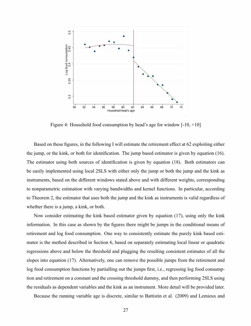
Figures 3 and 4 show changes in retirement rates and food consumption at 62, based on a ten-year

window at each side of the cutoff. The scatter plots in these �gures show sample averages by age.

Also shown are �tted quadratic regression lines above and below the cutoff age 62.14 As one can see,

the retirement rate has plausibly a small jump and may also have a small kink (slope change) at 62,

whereas the food consumption has a more obvious kink than a jump at the cutoff. In particular, the

age pro�le of food consumption jumps around a relatively �at line before age 62, but then steeply

declines afterwards.15 Since the data appear to be noisier at younger ages, a speci�cation considered

later incorporates variation in within cell sampling variances. Note that no particular jumps or kinks

are present in the retirement rate at 65.14These scatter plots are equivalent to histograms or bin average graphs that are recommended in the standard RD

literature (see, e.g., Imbens and Lemieux 2008 and Lee and Lemieux 2010), since the reported age is in years.15Questions regarding food consumption changed somewhat after 1997, and overall the food consumption data are

noisier for early waves of PSID, which may contribute to the observed larger variances at younger ages.

26

3.3

3.35

3.4

3.45

3.5

50 52 54 56 58 60 62 64 66 68 70 72Household head's age

Log 

food

 con

sum

ptio

n

Figure 4: Household food consumption by head's age for window [-10, +10]

Based on these �gures, in the following I will estimate the retirement effect at 62 exploiting either

the jump, or the kink, or both for identi�cation. The jump based estimator is given by equation (16).

The estimator using both sources of identi�cation is given by equation (18). Both estimators can

be easily implemented using local 2SLS with either only the jump or both the jump and the kink as

instruments, based on the different windows stated above and with different weights, corresponding

to nonparametric estimation with varying bandwidths and kernel functions. In particular, according

to Theorem 2, the estimator that uses both the jump and the kink as instruments is valid regardless of

whether there is a jump, a kink, or both.

Now consider estimating the kink based estimator given by equation (17), using only the kink

information. In this case as shown by the �gures there might be jumps in the conditional means of

retirement and log food consumption. One way to consistently estimate the purely kink based esti-

mator is the method described in Section 6, based on separately estimating local linear or quadratic

regressions above and below the threshold and plugging the resulting consistent estimates of all the

slopes into equation (17). Alternatively, one can remove the possible jumps from the retirement and

log food consumption functions by partialling out the jumps �rst, i.e., regressing log food consump-

tion and retirement on a constant and the crossing threshold dummy, and then performing 2SLS using

the residuals as dependent variables and the kink as an instrument. More detail will be provided later.

Because the running variable age is discrete, similar to Battistin et al. (2009) and Lemieux and

27

Milligan (2008), I adopt speci�cations based on age-cell means. In particular, the outcome model is

speci�ed as

YeX D �0 C �1eX C �2eX2 C �3ReX C e; (19)

where eX D X � 62, and represents the distance to the cutoff. YeX is the average logged food con-sumption in each age cell and ReX is the empirical probability of retirement, i.e., the observed fractionof household heads who are retired at each age. Both are indexed by eX to emphasize that they arede�ned as sample averages by age. As noted by Lemieux and Milligan (2008), the corresponding

regression estimates based on micro-data are identical to weighted estimates of equation (19) if the

weight used is the number of observations by age, while weighting only affects the ef�ciency, but not

the consistency of least squares estimation.16

The sample size in each age cell for the ten-year windows below and above the cutoff age 62

(covering 52 to 71) ranges from a minimum of 479 to a maximum of 868 observations. Table 1 shows

the number of observations at each age.

Table 1 Number of observations at each age

eX -10 -9 -8 -7 -6 -5 -4 -3 -2 -1No. ofobservations

868 831 763 725 678 655 609 572 552 578

eX 0 1 2 3 4 5 6 7 8 9No. ofobservations

527 520 530 517 576 538 488 483 489 479

Ideally observations of the running variable would be continuous, not discretized by year as in

Table 1. However, as discussed by Lee and Card (2008), given a discretely observed running variable,

if the deviations of the speci�ed approximating function from the true regression function can be taken

to be random speci�cation errors, then the point estimates will still be consistent, though calculation

of standard errors for micro-data regressions would then need to take into account the clustered nature

of these speci�cation errors at the cell level. They show that under certain conditions, robust standard

errors from this cell level regression are valid.16An alternative speci�cation would be to use year speci�c cell means and then include in the model year dummies.

However, since in this case cross-year variations are captured by those dummies, it would be similar to using averagesover all years. A small disadvantage of using year speci�c cell means is having to estimate year speci�c effects.

28

Corresponding to the food consumption equation (19), retirement is speci�ed as

ReX D 0 C 1eX C 2eX2 C 3T � C 4eXT � C u; (20)

where T � D 1.eX > 0/ is the crossing threshold dummy indicating exceeding the early retirement age.Based on the identi�cation theorems provided earlier, either 3 or 4 could be set to zero, depending

on whether the source of identi�cation is a jump or a kink. Allowing both 3 and 4 to be nonzero

permits identi�cation based on either a jump or a kink, or both.

Log food consumption and retirement are speci�ed in equations (19) and (20) as second order

polynomial regressions in eX . Given asymptotically shrinking bandwidth, these may be interpretedas nonparametric local quadratic regressions, as recommended by Porter (2003). Although in theory

one could include higher order polynomial terms, higher order terms are asymptotically unnecessary

for consistency, and empirically cause numerical multicollinearity issues, given the relatively small

number of age cell means used for estimation here.

For a given degree of polynomial, shrinking the bandwidth generally reduces bias (at the cost of

increasing variance by reducing the effective sample size). For example, although Figure 4 based

on a ten-year window looks like a quadratic form might not be a good �t for log food consumption

below the cutoff, when looking at a narrower window, say 8 or 6 years from the cutoff, the scatter

plot would be better �tted by simple quadratics. This is con�rmed empirically below, where quadratic

speci�cations are shown to provide good �t and yield estimates that are robust across speci�cations,

including varying window widths and kernel weights.

Using either only the jump or both the jump and the kink, equation (19) is estimated by a weighted

2SLS, with the �rst stage given by equation (20), where 4 is set to zero for the former. Using only the

kink, 3 is set to zero in equation (20), and YeX and ReX in these two equations are replaced by residualsfrom regressions of YeX and ReX on one and T �, respectively. This way, the jumps are partialled outfrom the conditional means of YeX and ReX , which guarantees that identi�cation comes from only thekink. They are then estimated similarly by a weighted 2SLS.17

17For the kink based estimator, if one restricts the second derivatives to be the same at each side of the threshold sothat the (residualized) retirement treatment equation does not include an interaction term between eX2 and T �, then theresulting 2SLS estimator would correspond directly to the estimator given by equation (17). Alternatively, one can includethis interaction term to allow the second derivatives to be different. Either way in existence of kinks, the resulting kinkestimator converges to the same limiting value (analogous to the way either local linear or local quadratic regressions willconsistently estimate the same regression slope). In most cases examined in this paper, the results are not very different,though including this interaction yields estimates that are slightly more stable across different windows widths.

29

In all the weighted 2SLS, each observation is weighted by 1=.1 C jeX j/, so the observation at thecutoff having eX D 0 is weighted by one, whereas those further away are weighted by values less

than one. This weighting gives the greatest in�uence to observations that are most informative about

the treatment effect, that is, the observations that are closest to the cutoff. This weighting also makes

each stage of the 2SLS equivalent to a local polynomial regression at the cutoff point, with the weights

corresponding to the kernel function.

Besides the above kernel weighting, I also try weighting each observations additionally by the

inverse sample standard deviation of the dependent variable YeX , log food consumption within eachage cell. This weighting scheme takes into account differences in the sampling variances of log food

consumption at different ages, as indicated by Figure 4. This weighting was used by Lemieux and

Milligan (2008) for RD estimation of the disincentive effects of social assistance. As shown below,

the results are not sensitive to the different choices of weighting.

Table 2 Estimated retirement effects on food consumption at age 62-(I)

Jump Kink Both jump and kink(1) (2) (1) (2) (1) (2)

[-6,+6] -0.191 -0.171 -0.221 -0.226 -0.181 -0.181(0.089)** (0.086)** (0.045)*** (0.043)*** (0.090)** (0.085)**

[-8,+8] -0.211 -0.198 -0.194 -0.200 -0.226 -0.215(0.089)** (0.085)** (0.035)*** (0.033)*** (0.087)*** (0.084)***

[-10,+10] -0.206 -0.194 -0.211 -0.216 -0.225 -0.215(0.080)*** (0.077)** (0.027)*** (0.026)*** (0.077)*** (0.075)***

Note: estimates are based on the 1994 - 2007 PSID data, with data from the recessionyears 2001 and 2003 omitted. (1) uses the inverse distance weighting; (2) adds the inversesampling standard deviation weighting. Using weight (1), the �rst stage F statistics rangefrom 35.64 to 12579.95. Using weight (2), the �rst stage F statistics range from 75.45 to15304.00. For all speci�cations, the instrumental variables are (jointly) signi�cant at the 1%level in the �rst stage regression of the 2SLS. Robust standard errors are in parentheses; *signi�cant at the 10% level, ** signi�cant at the 5% level, *** signi�cant at the 1% level.

Table 2 presents the main estimation results. Each estimate in Table 2, when multiplied by 100,

equals the estimated average percentage change in food consumption at retirement, when retirement

is caused by reaching the age at which one quali�es for social security bene�ts. The �rst two columns

present jump based estimates. The middle two columns present kink based estimates as discussed

above. The last two columns present estimates using both the jump and kink for identi�cation. By

Theorem 2 and the properties of the 2SLS weights discussed in Section 4, this estimator is valid

30

regardless whether there is a kink, a jump, or both. For each of these three estimators, Column (1)

uses the inverse distance weighting, and Column (2) uses both the inverse distance and the inverse

sampling standard deviation weighting as discussed above.

For all the speci�cations, the �rst stage regression of the 2SLS is highly signi�cant with instru-

mental variables that are (jointly) signi�cant at the 1% level. The estimates remain similar regardless

of whether identi�cation is based on the jump, the kink, or both. For example, when using a six-

year window (covering age 56 to 67) and inverse distance weighting, the estimated food consumption

drops based on the jump, the kink, or both, are 20.6%, 21.1%, and 21.5%, respectively. Note that

Theorem 2 shows that when there is a jump, the kink based estimator given by equation (17), the ratio

of two kinks, is valid only when the derivative of the treatment effect with respect to the cutoff age 62

is zero, i.e., the treatment effect does not vary linearly with age. The fact that these three estimators

all yield similar results therefore suggests that this derivative may be zero, as would be the case if the

retirement treatment effect is locally constant.

The results are also robust to different weightings. For example, by the kink based estimator and

the inverse distance weighting (marked by (1) in Table 1) the estimated food consumption drops are

21.1%, 19.4%, and 21.1% for the 6, 8, and 10 years windows, respectively, in contrast to 22.6%,

20.0%, and 21.6% based on the alternative weighting. In all speci�cations, estimates based on the

two different ways of weighting are within one standard error of each other. Furthermore, the results

are not very sensitive to different window widths. For example, using only the jump for identi�cation

and the inverse distance weighting, the estimated drops in food consumption for the 6, 8, and 10 years

windows are 19.1%, 21.1%, and 20.6%, respectively. Results based on alternative equivalence scales

are reasonably close. For example, when using another commonly used equivalence scale, the OECD

equivalence scale or the Oxford scale, the estimated retirement effects are between 15% and 22%

(Appendix B Table A1).18

Estimates in this paper are largely consistent with what is documented in the literature. For ex-

ample, Ameriks et al. (2007) �nd that a typical U.S. household experiences roughly a 20% fall in

consumption at retirement. Bernheim et al. (2001) estimate an average 10%�20% downward shift in

the consumption pro�le around the time of retirement based on the 1978-1990 PSID. Hurd and Ro-

hwedder (2005) estimate the decline at 15%�20% using data from the Health and Retirement Study18The OECD equivalence scale assigns a value of 1 to the �rst household member, of 0.7 to each additional adult and

of 0.5 to each child. The equivalence scale then equals the sum of these values across all household members.

31

(HRS) and from a supplemental survey to the HRS, the Consumption and Activities Mail Survey

(CAMS). More recently, using panel data from 1980 to 2000 Consumer Expenditure Survey (CEX),

Aguila, Attanasio, and Meghir (2010) �nd that food expenditure declines at retirement, but not non-

durable expenditure.

Table 3 Estimated retirement effects on food consumption at age 62-(II)

Jump Kink Both jump and kink(1) (2) (1) (2) (1) (2)

[-6,+6] -0.226 -0.228 -0.226 -0.227 -0.215 -0.219(0.088)** (0.083)*** (0.036)*** (0.035)*** (0.083)** (0.079)***

[-8,+8] -0.220 -0.241 -0.210 -0.212 -0.239 -0.224(0.080)*** (0.081)*** (0.027)*** (0.026)*** (0.085)*** (0.076)***

[-10,+10] -0.240 -0.242 -0.211 -0.211 -0.217 -0.222(0.079)*** (0.076)*** (0.021)*** (0.021)*** (0.079)*** (0.070)***

Note: estimates are based on the 1994 - 2007 PSID data, including data from the recessionyears 2001 and 2003. (1) uses the inverse distance weighting, (2) adds the inverse samplingstandard deviation weighting. Using weight (1), the �rst stage F statistics range from 96.89to 5273.45. Using weight (2), the �rst stage F statistics range from 116.82 to 6094.19. Forall speci�cations, the instrumental variables are (jointly) signi�cant at the 1% level in the�rst stage regression of the 2SLS. Robust standard errors are in parentheses. * signi�cant atthe 10% level; ** signi�cant at the 5% level;*** signi�cant at the 1% level.

For another robustness check, I re-estimate the model using all years' data from 1994 to 2007,

including those from the recession years 2001 and 2003. The results are presented in Table 3. The

estimated consumption drops are comparable to and are only slightly larger on average than the es-

timates reported in Table 2 where the recession year's data are omitted. It is plausible that food

consumption drops more at retirement during recessions than in other time periods.

Table 4 reports 2SLS and OLS regression results based on individual household micro-data in-

stead of cell means, using data either omitting the recession years (Sample (I) in Table 4) and not

omitting (Sample (II)). Since these are not cell mean data, the estimates are weighted only by the

inverse distance weighting, not by within cell standard deviations. The speci�cations are the same

as equations (19) and (20), except that year dummies are added as additional covariates in these two

equations. Note that use of age-cell means averages over, and hence smooths out, variation across

years, which is analogous to including year dummies in the micro-data regressions. The difference

is that estimating the year speci�c effects tends to increase the standard errors (see, e.g., Lee and

Lemieux, 2010). Not surprisingly, for all three window widths (6, 8, or 10 years from the cutoff), the

32

point estimates based on the micro-data 2SLS remain reasonably close to the cell-mean based esti-

mates, while the standard errors are much larger. These increased standard errors cause the estimated

retirement effects to become statistically insigni�cant at conventional signi�cance levels.

Table 4 Estimated retirement effect on food consumption based on micro-data

Sample (I) Sample (II)(a) (b) (c) (d) (a) (b) (c) (d)

[-6,+6] -0.258 -0.198 -0.273 0.006 -0.253 -0.223 -0.255 -0.010(0.304) (0.199) (0.297) (0.023) (0.333) (0.195) (0.322) (0.022)

[-8,+8] -0.261 -0.185 -0.282 0.003 -0.249 -0.214 -0.244 -0.011(0.265) (0.177) (0.246) (0.023) (0.285) (0.173) (0.261) (0.022)

[-10,+10] -0.231 -0.210 -0.251 0.002 -0.233 -0.216 -0.221 -0.012(0.202) (0.165) (0.209) (0.123) (0.250) (0.061) (0.221) (0.022)

Note: Sample (I) omits years 2001 and 2003 data; Sample (II) includes years 2001 and2003 data. (a) Jump based 2SLS; (b) Kink based (partialling out jumps) 2SLS; (c) Jumpand kink based 2SLS; (d) OLS. All speci�cations are weighted by the inverse distanceweight. Robust standard errors are in parentheses.

Estimates based on OLS are in striking contrast to those by IV 2SLS. OLS yields effects that are

mostly small and insigni�cant and also vary in signs depending on the samples used. In particular,

when using the sample that leaves out recession years, OLS estimates of retirement effects have

implausible positive signs.

To evaluate the plausibility of the RD assumptions, I examine whether the baseline covariates have

any unusual jumps or kinks at the cutoff. The RD modeling assumption implies that individuals do

not have precise manipulation of the running variable. If this is true, then there should be no sharp

changes at the cutoff age 62 in variables that are determined prior to the treatment. Otherwise it would

cast doubt on the validity of the smoothness assumption of potential outcomes as speci�ed in assump-

tion A1. I test smoothness of the conditional means of a battery of baseline covariates, conditional

on household head's age. The covariates tested include household head's gender, white/non-white,

Hispanic/non-Hispanic, marital status, wife's age, education (in years), and family size. As examples,

�gures 7 and 8 show the average values of wife's age and family size by head's age. One can see that

they both change smoothly with household head's age and there are no unusual jumps or kinks at 62.

Formally, this imprecise manipulation assumption can be tested by the method proposed by Lee

(2008) and Lee and Lemieux (2010). First choose covariates that are known to be unaffected by re-

tirement but are correlated with food consumption, and then test the null hypothesis of a zero average

33

5055

6065

70W

ife's

 age

50 52 54 56 58 60 62 64 66 68 70 72Household head's age

Figure 5: Wife's age by household head's age

effect on these pseudo outcomes by conducting parallel RD analyses, i.e., replacing the dependent

variable in the second stage of 2SLS with these covariates and performing similar 2SLS estimation.

The test results are reported in Appendix B Table A2. For all the covariates listed above, the coef�-

cients of retirement are not statistically signi�cant at any conventional levels and hence con�rm the

imprecise manipulation assumption.

I next test the smoothness of the density of age at the cutoff, though intuitively it is unlikely

that individuals could manipulate age to qualify for social security retirement bene�ts. Following

the general idea of the density test in McCrary (2008), I estimate a local regression the same as the

retirement equation except that the retirement rate ReX is now replaced by the fraction of observationsat each age. I then test the signi�cance of the estimated coef�cients of 1.eX > 0/ and eXT � to determinewhether there is a signi�cant jump or kink at the cutoff. This regression is intuitively equivalent to

graphing the fraction of each age (or a histogram) and inspecting if there are jumps or kinks at the

cutoff. As shown in Table A2 in Appendix B, the estimated coef�cients are not statistically signi�cant

at any conventional levels, thereby indicating no signi�cant jumps or kinks in the density of age at the

cutoff, which further con�rms the validity of the RD model here.

34

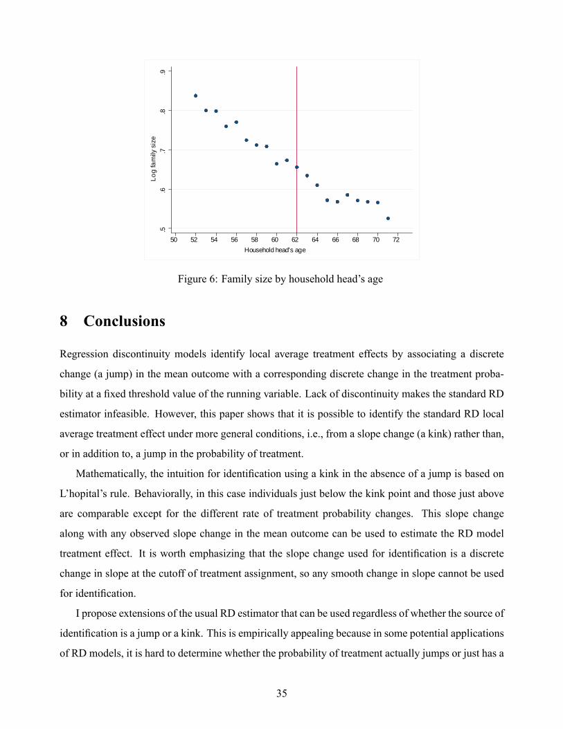
.5.6

.7.8

.9Lo

g fa

mily

 siz

e

50 52 54 56 58 60 62 64 66 68 70 72Household head's age

Figure 6: Family size by household head's age

8 Conclusions

Regression discontinuity models identify local average treatment effects by associating a discrete

change (a jump) in the mean outcome with a corresponding discrete change in the treatment proba-

bility at a �xed threshold value of the running variable. Lack of discontinuity makes the standard RD

estimator infeasible. However, this paper shows that it is possible to identify the standard RD local

average treatment effect under more general conditions, i.e., from a slope change (a kink) rather than,

or in addition to, a jump in the probability of treatment.

Mathematically, the intuition for identi�cation using a kink in the absence of a jump is based on

L'hopital's rule. Behaviorally, in this case individuals just below the kink point and those just above

are comparable except for the different rate of treatment probability changes. This slope change

along with any observed slope change in the mean outcome can be used to estimate the RD model

treatment effect. It is worth emphasizing that the slope change used for identi�cation is a discrete

change in slope at the cutoff of treatment assignment, so any smooth change in slope cannot be used

for identi�cation.

I propose extensions of the usual RD estimator that can be used regardless of whether the source of

identi�cation is a jump or a kink. This is empirically appealing because in some potential applications

of RD models, it is hard to determine whether the probability of treatment actually jumps or just has a

35

kink at the threshold. In these cases, treatment effects based on standard RD estimators would either

be weakly identi�ed, if the jump is small, or unidenti�ed if the jump is zero, regardless of how much

the slope changes. In contrast, this paper's estimators make use of any changes in either the intercept

or the slope of the treatment probability at a threshold of the running variable.

The identi�cation results in this paper can be intuitively interpreted using IV models. Just as

the standard fuzzy design RD estimator is numerically equivalent to an IV estimator, I show that the

proposed estimators are numerically equivalent to IV estimators. In particular, a kink in the treatment

probability provides an additional instrument that one can use to identify the RD treatment effect. If

there is no jump but a kink in the treatment probability, one would still be able to use this kink at

the threshold to identify the same local average treatment effect as would be identi�ed by a jump, if

the jump were to exist. A caveat is that this kink can be a valid instrument asymptotically only when

either there is no jump, or if there is a jump, � 0.c/ D 0 holds.

This paper proposes a local 2SLS estimator using both a jump and a kink as instruments. A nice

feature of this estimator is that it provides the type of weights Theorem 2 requires, so in practice,

one does not have to know beforehand whether there is a jump, or a kink, or both in the treatment

probability at the cutoff. This local 2SLS estimator yields consistent estimates for the RD local

average treatment effect regardless whether there is a jump, or a kink, and both.

All of the proposed estimators can be computed using just the estimated coef�cients from the same

local linear or polynomial regressions that are typically used to estimate standard RD models, so no

new estimation methods are required. As usual, one can alternatively do IV or 2SLS estimation using

observations in the neighborhood of the threshold to obtain not only point estimates of the treatment

effect, with an added advantage in this paper's context that 2SLS provides the type of weights that

some of the proposed estimators require.

The identi�cation results are applied to estimate the retirement impact on household food con-

sumption at the early retirement age 62 using the PSID data in the US. Graphical analyses show that

there might be a jump, a kink, or both in food consumption and retirement probabilities at 62. Es-

timators based on either a jump, or a kink, or both are performed. I show that all three yield very

similar estimates and that the results are robust to different window widths and weightings. Food

consumption is estimated to drop by about 15% to 23% when household heads retire. The estimates

are largely consistent with what is documented in the literature.

Similar to the standard RD identi�cation, this paper discusses the kink based identi�cation in a

36

static RD model setup. Extending the results to a dynamic setup to deal with, e.g., dynamic treatment

choices or dynamic treatment effects may be interesting directions of future research. Also given this

paper's results, it would be useful to explore identi�cation and estimation of other treatment related

parameters in the presence of kinks instead of jumps, such as the marginal policy effects of Carneiro,

Heckman, and Vytlacil (2010) and Heckman (2010).

9 Appendix A: Proofs

First note that for any x such that c� " � x � cC ", given Assumption A1, E .Y .1� D�/ j X D x/

and E .T .1� D�/ j X D x/ are continuously differentiable in the neighborhood of x D c, since

E .Y j X D x; D� D 0/, E .T j X D x; D� D 0/ and E .D� j X D x/ are assumed to be continuously

differentiable. The following proof will use these results.

PROOF of LEMMA 1:

Consider the conditional mean of Y in an RD model for a �xed threshold c,

E .Y j X D x/ D E�Y D� C Y

�1� D�

�j X D x

�D E

�Y j X D x; D� D 1

�E�D� j X D x

�C E

�Y�1� D�

�j X D x

�.

For any x > c, by the de�nition of compliers D� D 1, and the continuity of E .Y .1/ j X D x; D� D 1/

and E .Y .1� D�/ j X D x/, one has

gC.c/ D limx#cE .Y j X D x/

D E�Y .1/ j X D c; D� D 1

�E�D� j X D c

�C E

�Y�1� D�

�j X D c

�.

Similarly, for any x < c, by the de�nition of compliers D� D 1 and continuity of E .Y .0/ j X D x; D� D 1/

and E .Y .1� D�/ j X D x/, one has

g�.c/ D limx"cE .Y j X D x/

D E�Y .0/ j X D c; D� D 1

�E�D� j X D c

�C E

�Y�1� D�

�j X D c

�.

Therefore,

37

gC.c/� g�.c/ D E�Y .1/� Y .0/ j X D c; D� D 1

�E�D� j X D c

�.

E .Y .1/� Y .0/ j X D c; D� D 1/ is denoted as �.c/, so one has

gC.c/� g�.c/ D �.c/E�D� j X D c

�,

which is equation (1).

Similarly, given T D T D� C T .1� D�/ and the de�nition of compliers, one has

E .T j X D x/ D E�T j X D x; D� D 1

�E�D� j X D x

�C E

�T�1� D�

�j X D x

�D E

�T � j X D x; D� D 1

�E�D� j X D x

�C E

�T�1� D�

�j X D x

�.

E .T � j X D x; D� D 1/ D 1 for all x � c. Also E .T � j X D x; D� D 1/ D 0 for all x < c, so it

must hold in the limit as x " c. By continuity of E .T .1� D�/ j X D x/ and E .D� j X D x/, one

has

fC.c/� f�.c/ D limx#cE .T j X D x/� lim

x"cE .T j X D x/

D E�D� j X D c

�,

which is equation (2).

PROOF of THEOREM 1:

For t D 0; 1, de�ne the function G t .x/ by

G t .x/ D E�Y .t/ j X D x; D� D 1

�E�D� j X D x

�C E

�Y�1� D�

�j X D x

�:

Taking the ordinary derivative of this function gives

G 0t .x/ D@E .Y .t/ j X D x; D� D 1/ E .D� j X D x/

@xC@E .Y .1� D�/ j X D x/

@x:

This derivativeG 0t .x/ exists and is continuous at x D c because E .Y .t/ j X D x; D� D 1/, E .D� j X D x/,

38

and E .Y .1� D�/ j X D x/ are all continuously differentiable at x D c. It follows that

G 01 .c/� G00 .c/ D

@E .Y .1/� Y .0/ j X D c; D� D 1/ E .D� j X D c/@c

D � 0 .c/ E�D� j X D c

�C � .c/

@E .D� j X D c/@c

:

By the proof of Lemma 1 for x in the neighborhood of c we have g .x/ D G1 .x/ for x > c,

and by continuity of G 0t .x/ we have g0C .c/ D G 01 .c/. In the same way based on x 6 c we get

g0� .c/ D G 00 .c/, and so

g0C .c/� g0�.c/ D �

0 .c/ E�D� j X D c

�C � .c/

@E .D� j X D c/@c

: (21)

Similarly, we have

fC .c/ D limx#cE.T j X D x/ D E

�D� j X D c

�C E

�T�1� D�

�j X D c

�and

f� .c/ D limx"cE.T j X D x/ D E

�T�1� D�

�j X D c

�.

Given the continuous differentiability of E .T .1� D�/ j X D x/ and E .D� j X D x/ at the point

x D c, the ordinary derivatives of the right-hand side in the above two equations exist. So analogous

to the above analysis we obtain

f 0C .c/� f 0�.c/ D@E .D� j X D c/

@c. (22)

Given equations (21) and (22) and the assumption E .D� j X D c/ D 0, one has

g0C .c/� g0� .c/ D � .c/

�f 0C .c/� f 0�.c/

�, (23)

and so

� .c/ Dg0C .c/� g0� .c/f 0C .c/� f 0�.c/

.

Note that the above can be alternatively shown by L'hopital's rule. To see this, let B .x/ D

G1 .x/ � G0 .x/ for all x in the neighborhood of c. Similarly, let p .x/ D E .D� j X D x/. By

39

Assumption A1, both B .x/ and p .x/ are continuously differentiable.

From the above, one has B .c/ D G1 .c/�G0 .c/ D gC .c/� g� .c/ and p .c/ D fC .c/� fC .c/,

as well as B 0 .c/ D G 01 .c/�G00 .c/ D g

0C .c/� g0� .c/ and p0 .c/ D f 0C .c/� f 0� .c/. Lemma 1 shows

B .c/ D � .c/ p .c/, so given p .c/ D 0, one has B .c/ D � .c/ p .c/ D 0. Then

� .c/ Dlimx!c B .x/limx!c p .x/

Dlimx!c B 0 .x/limx!c p0 .x/

DB 0.c/p0.c/

Dg0C .c/� g0� .c/f 0C .c/� f 0� .c/

,

where the second equality follows from L'hopital's rule, and the third from the continuous differen-

tiability of B .x/ and p .x/.19

PROOF of COROLLARY 1:

If there is a jump, i.e, the identi�ed difference fC.c/ � f�.c/ is nonzero, then �.c/ is identi�ed

by equation (4). Alternatively, if there is no jump ( fC.c/� f�.c/ D 0), then by Assumption A2 there

must be a kink. So by Theorem 1 �.c/ is identi�ed by equation (5).

PROOF of THEOREM 2:

Suppose �rst that there is a jump, fC .c/� f� .c/ 6D 0, then

limn!1

gC .c/� g� .c/C wn�g0C .c/� g0� .c/

�fC .c/� f� .c/C wn

�f 0C .c/� f 0� .c/

� D gC .c/� g� .c/fC .c/� f� .c/

D �.c/.

Alternatively, suppose there is no jump, fC .c/� f� .c/ D 0 and gC .c/�g� .c/ D �.c/ . fC .c/� f� .c// D

0, thengC .c/� g� .c/C wn

�g0C .c/� g0� .c/

�fC .c/� f� .c/C wn

�f 0C .c/� f 0� .c/

� D wn�g0C .c/� g0� .c/

�wn�f 0C .c/� f 0� .c/

� D �.c/;where the last equality follows from Theorem 1. Since this equality holds for all n, it must hold in the

limit as n!1.

PROOF of COROLLARY 2:

For convenience, I will continue to use B .c/, p .c/, B 0.c/, and p0.c/ as in the proof of Theorem

1. If there is no jump, i.e., p.c/ D 0 and hence B.c/ D � .c/ p .c/ D 0, by Assumption A2, there is a19These derivations involve conditioning on set of measure zero. However, issues of nonuniqueness of the limiting

argument (the Borel-Kolmogorov paradox) do not arise here, since our methodology consists only of transformations ofsmooth conditional expectation functions.

40

kink. Then Theorem 1 gives

� .c/ DB 0 .c/p0 .c/

DB .c/C wB 0 .c/p .c/C wp0 .c/

:

Now consider the case where � 0 .c/ D 0. By equations (21) and (22), if � 0 .c/ D 0 then B 0 .c/ D

� .c/ p0 .c/, and in addition it has already been shown that B .c/ D � .c/ p .c/ with equations (1) and

(2). Taking a weighted sum of these two equations gives B .c/ C wB 0 .c/ D � .c/ .p .c/ C wp0 .c//.

Then

� .c/ DB .c/C wB 0 .c/p .c/C wp0 .c/

.

The denominator of this equation is nonzero, since by Assumption A2 either p .c/ or p0 .c/ is nonzero.

PROOF of THEOREM 3:

Similar to Theorem 2, suppose �rst that there is a jump, p 6D 0, then

limn!1

B C !n .2qC � Dp/p C !n

�2q2 � rp

� DBpD �.c/.

Alternatively, suppose there is no jump, p D 0, and hence B D �.c/p D 0, so

B C !n .2qC � Dp/p C !n

�2q2 � rp

� D!n .2qC � Dp/!n�2q2 � rp

� D CqD �.c/,

where the last equality follows from Theorem 1. It holds for all n, so it holds in the limit as n!1.

PROOF of COROLLARY 3:

Use the notation in the proof of Theorem 1, and for simplicity replace B.c/ and p.c/ with B and

p, respectively. From Lemma 1,

B D � .c/ p:

Twice differentiability gives

B 0 D � 0 .c/ p C � .c/ p0; (24)

B 00 D � 00 .c/ p C 2�.c/0 p0 C �.c/p00: (25)

41

Recall by notation in the text B 0 D C , p0 D q, B 00 D D, and p00 D r . If there is no jump, p D 0.

By Assumption A2, there is a kink, so p0 D q 6D 0. From Theorem 1, one has

� .c/ DB 0

p0DCqDB C w .2qC � Dp/p C w

�2q2 � rp

�for any w 6D �p=

�2q2 � rp

�. The last equality follows from p D 0 and hence B D � .c/ p D 0.

If � 00 .c/ D 0, then solving for � .c/ from equations (24) and (25) gives

� .c/ D2qC � Dp2q2 � rp

.

Also if there is a jump, the standard RD estimator applies, � .c/ D Bp . By the rule of fraction,

one has

� .c/ DB C w .2qC � Dp/p C w

�2q2 � rp

�for any w 6D �p=

�2q2 � rp

�.

The same procedure can be applied to cases where the d-th derivative � .d/ .c/ D 0 for any �nite

positive integer d. Keep taking derivatives on both sides of B D � .c/ p, until the d-th derivative.

With the system of d equations and � .d/ .c/ D 0, one can back out � .c/, as the system of equations

are recursive in nature.

42

10 Appendix B: Tables

Table A1 Estimated retirement effects on food consumption at age 62 - (III)Jump Kink Both jump and kink(1) (2) (1) (2) (1) (2)

[-6,+6] -0.186 -0.176 -0.175 -0.180 -0.193 -0.184(0.097)* (0.093)* (0.048)*** (0.046)*** (0.096)** (0.091)**

[-8,+8] -0.212 -0.200 -0.150 -0.155 -0.223 -0.212(0.095)** (0.091)** (0.037)*** (0.036)*** (0.092)** (0.088)**

[-10,+10] -0.205 -0.194 -0.166 -0.170 -0.219 -0.210(0.085)** (0.082)** (0.029)*** (0.028)*** (0.081)*** (0.079)***

Note: estimates are based on the 1994 - 2007 PSID data, not including the recession years2001 and 2003. Food consumption is scaled by an alternative OECD equivalence scale. (1)uses the inverse distance weighting; (2) uses both the inverse distance and inverse samplingstandard deviation weighting. Using weight (1), the �rst stage F statistics range from 63.44to 12579.95. Using weight (2), the �rst stage F statistics range from 74.03 to 15122.38. Forall speci�cations, the instrumental variables are (jointly) signi�cant at 1% level in the �rststage regression of the 2SLS. Robust standard errors are in the parentheses. * signi�cant atthe 10% level; ** signi�cant at the 5% level; *** signi�cant at the 1% level.

Table A2 The smoothness of conditional means of covariates and density of ageRetirement effects on base-line covariate:Male 0.089 (0.066)White -0.060 (0.058)Married 0.112 (0.069)Wife's age 1.197 (1.000)Hispanic -0.031 (0.037)Education 1.041(0.705)Family size -0.014 (0.061)

Density of household head's age:Jump -0.000 (0.002)Kink 0.001 (0.001)Note: Robust standard errors are in the parentheses; All the estimatesare not statistically signi�cant at the conventional signi�cance levels;Estimation is based on a 10 years window with the inverse densityweighting and inverse sampling standard deviation weighting.

References

[1] Aguila, E., O. Attanasio, and C. Meghir (2010), "Changes in consumption at retirement: evi-

dence from panel data," forthcoming, The Review of Economics and Statistics.

43

[2] Ameriks, J., A. Caplin, and J. Leahy (2007), "Retirement Consumption: Insights from a Survey,"

The Review of Economics and Statistics 89, 265-274.

[3] Angrist, J. D. and J.-S. Pischke (2008), Mostly Harmless Econometrics: An Empiricist's Com-

panion, Princeton University Press.

[4] Battistin E., A. Brugiavini, E. Rettore, and G. Weber (2009), "The Retirement Consumption

Puzzle: Evidence from a Regression Discontinuity Approach," American Economic Review 99,

2209�2226.

[5] Bernheim, B. D., J. Skinner, and S. Weinberg (2001), "What Accounts for the Variation in

Retirement Wealth Among U.S. Households?" American Economic Review 91, 1�26.

[6] Card, D., C. Dobkin, and N. Maestas (2008), "The Impact of Nearly Universal Insurance Cov-

erage on Health Care Utilization: Evidence from Medicare," American Economic Review 98,

2242�2258.

[7] Card, D., D. S. Lee and Z. Pei (2009), "Quasi-Experimental Identi�cation and Estimation in the

Regression Kink Design," Princeton University, WP # 553.

[8] Carneiro, P., J. J. Heckman, and E. Vytlacil, (2010), "Evaluating Marginal Policy Changes and

the Average Effect of Treatment for Individuals at the Margin," Econometrica 78, 377�394.

[9] Citro, C. F. and R. T. Michaels (1995), Measuring Poverty: A New Approach, C. F. Citro and R.

T. Michaels (Eds.) National Academy Press, 161-162.

[10] Davidson, R. and J. G. MacKinnon (1993), Estimation and Inference in Econometrics, Oxford

University Press.

[11] Dong, Y. (2012), "Regression Discontinuity Applications with Rounding Errors in the Running

Variable," University of California Irvine working paper numer 11-12-06

[12] Guryan, J. (2003), "Does Money Matter? Regression-Discontinuity Estimates from Education

Finance Reform in Massachusetts," National Bureau of Economic Research, WP8269.

[13] Hahn, J., P. E. Todd, and W. van der Klaauw (2001), "Identi�cation and Estimation of Treatment

Effects with a Regression-Discontinuity Design," Econometrica 69, 201�09.

44

[14] Heckman, J. J. (2010), "Building Bridges Between Structural and Program Evaluation Ap-

proaches to Evaluating Policy," Journal of Economic Literature 48, 356-398.

[15] Hurd, M., and S. Rohwedder (2005), "The Retirement-Consumption Puzzle: Anticipated and

Actual Declines in Spending at Retiremen," RAND Labor and Population working paper series

WR-242.

[16] Imbens, G. W. and K. Kalyanaraman (2012), "Optimal Bandwidth Choice for the Regression

Discontinuity Estimator," Review of Economic Studies 79(3), 933-959

[17] Imbens, G.W. and T. Lemieux (2008), "Regression Discontinuity Designs: A Guide to Practice,"

Journal of Econometrics 142, 615�35.

[18] Imbens, G. W. and J. M. Wooldridge (2009), "Recent Developments in the Econometrics of

Program Evaluation," Journal of Economic Literature 47, 5�86.

[19] Jacob, B. A., and L. Lefgren (2004), "Remedial Education and Student Achievement: A

Regression-Discontinuity Analysis," The Review of Economics and Statistics 86, 226�244.

[20] Lee, D. S. (2008), "Randomized Experiments from Non-random Selection in U.S. House Elec-

tions," Journal of Econometrics, 142(2), 675�697.

[21] Lee, D. S. and T. Lemieux (2010), "Regression Discontinuity Designs in Economics," Journal

of Economic Literature 48, 281�355.

[22] Lemieux, T. and K. Milligan (2008), "Incentive effects of social assistance: A regression dis-

continuity approach," Journal of Econometrics 142, 807�828.

[23] Ludwig, J., and D. L. Miller (2007), �Does Head Start Improve Children's Life Chances? Evi-

dence from a Regression Discontinuity Design,� Quarterly Journal of Economics, 122, 159�208.

[24] Mariger, R. (1987), "A Life-Cycle Consumption Model with Liquidity Constraints: Theory and

Empirical Results," Econometrica 55, 533�557.

[25] McCrary, J. (2008), "Manipulation of the running variable in the regression discontinuity design:

A density test," Journal of Econometrics 142,698�714.

45

[26] Nielsen, H. S., T. Sorensen, and C. R. Taber (2009), "Estimating the Effect of Student Aid on

College Enrollment: Evidence from a Government Grant Policy Reform,� American Economic

Journal: Economic Policy," forthcoming.

[27] Porter, J. R. (2003), "Estimation in the Regression Discontinuity Model," Unpublished Manu-

script.

[28] Rubin, D. B. (1974), "Estimating Causal Effects of Treatments in Randomized and Nonrandom-

ized Studies," Journal of Educational Psychology 66, 688�701.

[29] Simonsen, M., L. Skipper, and N. Skipper (2009), �Price Sensitivity of Demand of Prescrip-

tion Drugs: Exploiting a Kinked Reimbursement Scheme,� University of Aarhus Economics

Working Papers no. 2010-03.

[30] Thistlethwaite, D. L. and D. T. Campbell (1960), "Regression-Discontinuity Analysis: An Al-

ternative to the Ex-Post Facto Experiment," Journal of Educational Psychology 51, 309�317.

46