Quantitative Finance, 2014Vol. 14, No. 8, 1427–1444, http://dx.doi.org/10.1080/14697688.2013.830320

Jump detection with wavelets for high-frequencyfinancial time series

YI XUE†, RAMAZAN GENÇAY‡§∗ and STEPHEN FAGAN‡¶

†Department of Finance, School of International Trade and Economics, University of International Business and Economics,#10 Huixin Dongjie, Chaoyang District, Beijing, China

‡Department of Economics, Simon Fraser University, 8888 University Drive, Burnaby, British Columbia, V5A 1S6, Canada§Rimini Center for Economic Analysis, Rimini, Italy

(Received 6 December 2011; accepted 25 July 2013)

This paper introduces a new nonparametric test to identify jump arrival times in high frequencyfinancial time series data. The asymptotic distribution of the test is derived. We demonstrate that thetest is robust for different specifications of price processes and the presence of the microstructurenoise. A Monte Carlo simulation is conducted which shows that the test has good size and power.Further, we examine the multi-scale jump dynamics in US equity markets. The main findings are asfollows. First, the jump dynamics of equities are sensitive to data sampling frequency with significantunderestimation of jump intensities at lower frequencies. Second, although arrival densities of positivejumps and negative jumps are symmetric across different time scales, the magnitude of jumps isdistributed asymmetrically at high frequencies. Third, only 20% of jumps occur in the trading sessionfrom 9:30AM to 4:00 PM, suggesting that illiquidity during after-hours trading is a strong determinantof jumps.

Keywords: Jump detection; Wavelets; Directional jumps; Positive jumps; Negative jumps

JEL Classification: G10, G11, D43, D82

1. Introduction

In the last two decades, a substantial amount of empiricalevidence has been found to support the existence of surpriseelements, commonly called jumps, in financial time series. Itis well understood that compared to continuous price changes,jumps have distinctly different modeling, inference, and testingrequirements. These differences impact how we perform manyimportant financial tasks such as valuing derivative securities,inferring extreme risks, and determining optimal portfolio allo-cations. Thus, understanding what drives jumps in underlyingsecurities, how to characterize jumps both theoretically andempirically, and having efficient tests available for jumps thatare sufficiently robust to withstand mis-specification and smallsample bias is imperative.

This paper proposes a new method to estimate a jump’slocation and size, as well as the number of jumps in a giventime interval from high frequency data. In addition to providinga practical jump detection criterion, we derive the asymptoticdistribution of the test statistic and demonstrate that the test hasgood size and power properties. Our methodology is based ona wavelet decomposition of the data and we show that the test

∗Corresponding author. Email: rgencay@sfu.ca¶Current address: BlackRock, Inc., New York, NY, USA.

of Lee and Mykland (2008) is a special case of a wavelet-typetest. Additionally, we show that when a wavelet filter withless leakage is used, the performance of the test improves.‖This improvement originates from the fact that the waveletcoefficients with less leakage are better able to isolate thehigh frequency components of the price process where jumps,when they occur, will dominate other components such ascontinuous changes and microstructure effects. Thus, we canavoid identifying spurious jumps while preserving power indetecting true jumps.††

A substantial amount of research has been dedicated todetecting jumps in asset prices. Among previous studies,Andersen et al. (2003) proposed a method using a jump-robustestimator of realized volatility. Barndorff-Nielsen andShephard (2004, 2006) proposed a bi-power variation (BPV)measure to separate the jump variance and diffusive variance.Lee and Mykland (2008) developed a rolling-based nonpara-metric test for jumps and a method for estimating jump sizes

‖A filter with less leakage is one that is closer to being an ideal band-pass filter.††Spurious jumps are observations where no jump actually occurred,but the test incorrectly identified one to have occurred due to largemovements originating from the presence of microstructure effects orlarge spot volatility.

© 2013 Taylor & Francis

Dow

nloa

ded

by [

Sim

on F

rase

r U

nive

rsity

] at

18:

20 1

6 A

ugus

t 201

4

1428 Y. Xue et al.

and jump arrival times. Jiang and Oomen (2008) proposed ajump test based on the idea of a ‘variance swap’ and explicitlyaccounted for market microstructure effects. Johannes (2004)and Dungey et al. (2009) found significant evidence for jumpsin US treasury bond prices and rates. Piazzesi (2003) demon-strated that jump modeling leads to improved bond pricing inthe US treasury market. Andersen et al. (2007) showed thatincorporation of jump components could improve the fore-casting of return volatility. Fan and Wang (2007) showed thatwhen market returns contain jumps, separating the variation inreturns into jump and diffusion components is important forefficient estimation of realized volatility.

Wavelets can be a powerful tool for detecting jumps fortwo reasons. First, the ability of wavelets to decompose noisytime series data into separate time-scale components helpsus to distinguish jumps from continuous price changes andmicrostructure effects.The high-frequency wavelet coefficientsat jump locations are larger than other wavelet coefficients dueto the fact that wavelet coefficients decay at a different ratefor continuous processes and jump processes. In a given smalltime interval, changes in continuous price processes are closeto zero while jumps are not.† Such information is containedin wavelet coefficients at the jump locations (see Wang (1995)and Fan and Wang (2007)).‡ Second, estimation of jump sizeis closely related to the estimation of integrated volatility. AsFan and Wang (2007) demonstrated, wavelets allow superiorestimation of the integrated volatility, which can improve theefficiency of the estimation of jump size.

This paper implements our wavelet jump test to examinethe jump dynamics of three US equities and finds that theirestimated jump dynamics are sensitive to the data samplingfrequency. This emphasizes the importance of an optimal sam-pling frequency to extract full jump dynamics. Our resultssuggest that the popular choice of 5-min sampling frequencymay neglect a large proportion of jump dynamics embeddedin transaction prices. Additionally, although jump arrival den-sities of positive jumps and negative jumps are symmetricacross time scales, the magnitude of jumps is asymmetricallydistributed at high frequencies. This suggests that a skeweddistribution for the magnitude of jumps should be employed inrisk management and asset pricing practices for high frequencytrading. Finally, only 20% of jumps occur in the trading sessionfrom 9:30 AM to 4:00 PM, suggesting that illiquidity duringafter-hours trading is a strong determinant of jumps.

Overall, the main contributions of the paper are as follows.First, a nonparametric jump detection test based on wavelettransformations is proposed and the asymptotic distribution ofthe test statistic is established. This test is shown to improvejump detection by avoiding the identification of spurious jumpsand providing improved estimation of jump locations. Second,we show that the jump detection test is robust in the presence ofmicrostructure noise. Finally, the empirical implementation of

†Continuous price processes include cusps which are nondifferen-tiable kinks connecting two differentiable intervals. Differences in aprice process at a heavy cusp converge to zero much more slowlythan at a differentiable point. In the limit cusps are jumps.‡Wang (1995) and Fan and Wang (2007) proposed a wavelets-based procedure using the different convergence rates of waveletcoefficients with or without jumps. In addition to jump size,Fan and Wang (2007) could estimate the number of jumps and anestimated interval of jump location.

the wavelet test in US equity markets demonstrates a dramaticchange of jump dynamics across time scales, the asymmetricdistribution of jump magnitudes at high frequencies and theoccurrence of the majority of jumps outside of the primarytrading session.

In Section 2, we provide the theoretical framework for jumpdetection in the absence of microstructure effects and introducethe wavelet-based jump test statistic. The asymptotic distribu-tion of the test statistic follows a scaled normal distributionand the scalar is determined by the properties of the waveletfilter. Section 3 extends the framework to investigate the per-formance of the test in the presence of microstructure effects.We show that the asymptotic distribution of the test statisticunder the null hypothesis remains the same. Section 4 presentsMonte Carlo simulation results which demonstrate the finitesample behavior of the proposed test. We show that the test hasdesirable size and power in small samples. Section 5 discussesthe empirical examination of jump dynamics in equity markets.

2. The jump test without microstructure noise

Wavelets have been shown to be useful for jump detection whenprices are following a jump-diffusion process. Fan and Wang(2007) used the localization property of wavelet expansion todetect jumps. This property entails that if a function containsa jump but is otherwise Holder-continuous,§ then the waveletcoefficients of the high-pass filter close to the jump point decayat order 2

12 j , where j is a scale of the wavelet decomposition.

If there is no jump, the wavelet coefficients of the high passfilter decay at order 2

32 j . This special feature was used to

separate jumps from the continuous and microstructure noisecomponents of the process (Wang 1995).

Although Fan and Wang (2007) showed the effectivenessof the wavelets method for jump detection with a diffusionprocess convincingly, the distributional properties of the jumpdetection test statistic were not formally defined. Additionally,because a discrete wavelet transformation (DWT) was appliedto the data, the jump location could only be estimated with aninformational loss in time domain.

This paper proposes a framework for jump detection usingwavelets and formally develops the test statistic. Before wemathematically define this jump detection statistic JW , wedescribe the basic intuition behind the proposed detection tech-nique. Imagine that asset prices evolve continuously over time,but due to an announcement or some other informational shock,a jump in prices occurs at time t . Given the additive nature ofthe jump, we expect to see the mean level of the price processabruptly shift. The large return at this point could be due toany combination of the drift, diffusion, or jump components ofthe price process, but as our sampling frequency gets higher,the contribution of the drift and diffusion components getssmaller. The contribution of an instantaneous jump howeverwill not get smaller. Thus, we should expect to see a relativelylarge absolute value for the return rt at the jump location.

§A function g : Rd → R is said to be Holder-continuous if thereexist constants C and 0 ≤ E ≤ 1 such that for all u and v in Rd :|g(u)− g(v)| ≤ C ||u − v||E .

Dow

nloa

ded

by [

Sim

on F

rase

r U

nive

rsity

] at

18:

20 1

6 A

ugus

t 201

4

Jump detection with wavelets for high-frequency financial time series 1429

This intuitive description of a jump test transfers easily toone using wavelet coefficients rather than returns. Like returns,wavelet coefficients contain information on differenced prices.Unlike returns however, wavelet coefficients break the priceseries down into different components which correspond todifferent frequencies.Atechnical introduction to wavelet trans-formations is presented in Appendix A1. Since jumps are un-expected and instantaneous, their contribution will be cap-tured in the wavelet coefficients corresponding to the highestfrequency. Using wavelet coefficients from this scale shouldtherefore provide a cleaner jump test statistic since low-frequency components have been filtered out. Thus, our jumptest is based on the expectation that we should see a relativelylarge wavelet coefficient at jump locations.

If prices were continuously observed, jumps would be easyto identify. However, with discrete price observations, we canobserve a large price change even without a jump if spot volatil-ity is large enough. Thus, it is difficult to distinguish whetherthe observed large movement in prices is due to a jump inprice process or a volatility of large magnitude. High fre-quency price data reduces the severity of this problem, butsince spot volatility may vary over time, we normalize theabsolute value of wavelet coefficients by the estimated spotvolatility. To get a consistent estimate of the spot volatility inthe presence of jumps, we apply the BPV estimator suggestedby Barndorff-Nielsen and Shephard (2004).

Furthermore, we use the maximum overlap discrete wavelettransformation (MODWT) instead of DWT. MODWT gener-ates an equal number of wavelet coefficients (high pass filter)as the original data series. Combined with zero phase correc-tion, the locations of the wavelet coefficients naturally revealinformation concerning the original data in the time domain.Thus, the jump location detection is reduced to a jump detectionproblem.

2.1. Definition of the test

We employ a one-dimensional asset return process. Let thelogarithm of the market price of the asset be Pt = log St

where St is the asset price at time t . When there are no jumpsin the market price, Pt is represented as

Pt =∫ t

0μsds +

∫ t

0σsdWs (1)

where the two terms correspond to the drift and diffusion com-ponents of Pt . In the diffusion term, Wt is a standard Brownianmotion, and the square root of the diffusion variance σ 2

t iscalled spot volatility. Equivalently, Pt can be characterized as

d Pt = μt dt + σt dWt . (2)

When there are jumps, Pt is given by

Pt =∫ t

0μsds +

∫ t

0σsdWs +

Nt∑l=1

Ll (3)

where Nt represents the number of jumps in Pt up to time tand Ll denotes the jump size. Equivalently, Pt can be modeledas

d Pt = μt dt + σt dWt + Lt d Nt (4)

where Nt is a counting process that is left unmodeled. Weassume jump sizes Ll are independently and identically dis-tributed. They are also independent of other random compo-nents Wt and Nt .

Observations of Pt , the log price, are only available at dis-crete times 0 = t0 < t1 < t2 < . . . < tn = T . For simplicity,we assume observations are equally spaced: �t = ti − ti−1.Following Lee and Mykland (2008), we impose the followingassumptions on price processes throughout the paper: For anysmall ε > 0,

A1 supi supti ≤u≤ti+1|μu − μti | = Op

(�t

12 −ε)

A2 supi supti ≤u≤ti+1|σu − σti | = Op

(�t

12 −ε)

The assumption A1 and A2 can be interpreted as the driftand diffusion coefficients not changing dramatically over ashort time interval.† Formally, this states that the maximumchange in mean and spot volatility in a given time interval isbounded above. The assumptions A1 and A2 guarantee that theavailable discrete data are reasonably well-behaved such thatthe data are a good approximation of the continuous processof the underlying asset. The availability of high frequencyfinancial data allows us to improve the approximation of thecontinuous underlying asset process using discrete data.

Now, let P1,t be the wavelet coefficients of Pt = log(St ) fora first scale MODWT. We define the test statistic as JW , whichtests whether a jump occurs at time ti for i = 3, . . . , T as

JW (i) = P1,ti

σti−1

(5)

where σ 2ti−1

= 1i−2

i−1∑k=2

|P1,tk ||P1,tk−1 |.Following Lee and Mykland (2008), we employ a BPV

method to estimate the integrated volatility of the underlyingprocess. However, there are two major differencesbetween our approach and theirs. First, we apply BPV onwavelet transformed data (wavelet coefficients calculated fromthe raw data) rather on the raw data. Wavelets have the ability todecompose the raw data into high frequency components andlow frequency components. Since jumps are unexpected andinstantaneous, we believe that jump dynamics should be con-tained in the high frequency components of prices. By usingwavelet coefficients rather than returns, we rely on the abilityof wavelet filter to extract the return dynamics to estimate thehigh-frequency component of instantaneous volatility. Second,we use all of the data points available up the jump locationrather than a choice of window size K as in Lee and Mykland(2008). The choice of K is to minimize the impact of the jumpson the estimation of the instantaneous volatility within thewindow. As argued in Fan and Wang (2007), wavelets havethe ability to estimate the instantaneous volatility with thepresence of the jumps. We conjecture that using more sophisti-cated wavelet filters, e.g. S8 filter rather Haar filter, can helpus to detect jumps in the stochastic volatility framework. Thatis, we choose a wavelet filter rather window size to minimize

†Following Pollard (2002) and Lee and Mykland (2008), we use Opnotation throughout this article to mean that, for random vectors{Xn}, and non-negative random variable {dn}, Xn = Op(dn),if for each δ > 0, there exists a finite constant Mδ such thatP(|Xn | > Mδdn) < δ.

Dow

nloa

ded

by [

Sim

on F

rase

r U

nive

rsity

] at

18:

20 1

6 A

ugus

t 201

4

1430 Y. Xue et al.

the impact of the jumps on the estimation of the instantaneousvolatility.

There are alternative methods for estimating the integratedvolatility including the two scale realized volatility estima-tors (TSRV) (Zhang et al. 2005) and the multi-scale realizedvolatility estimators (MSRV) (Zhang 2006). However,Barndorff-Nielsen and Shephard (2004) demonstrated that thepresence of jumps will change the asymptotic behavior of thesetests. Additionally, they showed that a BPV estimator is robustin the presence of the jumps.

2.2. A general filter case

In this section, we demonstrate the test statistics with ageneral wavelet filter, i.e. we L wavelet filter coefficients,h0, . . . , hL−1, such that

∑L−1l=0 hl = 0. Under the null hypoth-

esis that no jump occurs at time ti , as �t goes to zero, JW (i)should converge to a normal distribution under the assumptionsof A1 and A2. Theorem 1 demonstrates the distribution ofthe proposed statistic in the case of MODWT with a generalfilter. As argued in Lee and Mykland (2008), when workingwith high-frequency data, the drift (of order dt) is mathemati-cally negligible compared to the diffusion (of order

√dt) and

the jump component (of order 1). In fact, the drift estimateshave higher standard errors, so that they cause the precisionof variance estimates to decrease if included in the varianceestimation. Therefore, we assume zero drift in this study.†

Theorem 1 Assuming zero drift and constant spot volatilityin the underlying price process and assuming A1 and A2 aresatisfied, if there is no jump in (ti−1, ti ), as �t → 0

supi |JW (i)− JW (i)| = Op

(�t

32 −δ−ε) ,

where δ satisfies 0 < δ < 3/2 and JW (i) = Ui

d. (6)

where Wt follows a Brownian motion process. AndUi = 1√

�t(Wti − Wti−1), a standard normal variable, and

a constant d =√

E[B PVG ]√∑L−2l=0 (

∑lj=0 h j )

2, where

E[B PVG ]

=∫ ∞

−∞. . .

∫ ∞

−∞E[B PVG |x1, . . . , xL−2]φ(x1)

. . . φ(xL−2)dx1 . . . dxL−2,

E[B PVG |r1, . . . , rL−2]

= 2σ 2 f

⎛⎝−∑L−2l=1

(∑lj=0 h j

)(rL−l−l)

h0

⎞⎠× f

⎛⎝−∑L−3l=0

(∑lj=0 h j

)(rL−l−l)(∑L−2

j=0 h j

)⎞⎠ ,

†We do study the statistics under non-zero drift case by simulationsand demonstrate that the performance of the test is not changed undernon-zero drift case.

where f (a) = 2φ(a)+2a�(a)−a, and rt s are independentlyand identically distributed (iid) standard normal variables.

Comments:

(1) The distribution of the test statistic is asymptoticallynormally distributed.

(2) Since JW (i) is asymptotically independent and nor-mally distributed over time, one can easily use ajoint normal distribution of the test statistics to detectmultiple jumps.

(3) In addition, the scaling factor d only depends on thewavelet filter coefficients. That is, when a particularwavelet filter is used, d can be computed based onthe values of hls.

Next, we demonstrate the implementation of the proposedtest using two popular wavelets filters, i.e. Haar filter (pro-posed by Haar (1910)) and D4 filter (proposed by Daubechies(1988)).‡ If we implement the jump detection test using aHaar filter, i.e. h1 = 1/2, h2 = −1/2. In this case, wehave the following proposition which is a direct applicationof Theorem 1.

Proposition 2 (Haar filter case) Assuming zero drift andA1 and A2 are satisfied. If there is no jump in (ti−1, ti ), as�t → 0,

supi |JW (i)− JW (i)| = Op

(�t

32 −δ−ε) ,

where δ satisfies 0 < δ < 3/2 and JW (i) = Ui

d. (7)

where Wt follows a Brownian motion process. Here Ui =1√�t(Wti −Wti−1), a standard normal variable, and d = E[|Ui |]

=√

2√π

is a constant.

It is worth noting that the test statistics JW (i) in Proposition 2,i.e. the test statistics in the case of Haar filter, is equivalent totest statistics proposed in Lee and Mykland (2008).

Similarly, in the case of D(4) filter , i.e. h1 = 18 (1 − √

3),h2 = 1

8 (√

3 − 3), h3 = 18 (3 + √

3), h4 = 18 (−1 − √

3), wecan show that

Proposition 3 (D4 filter) Assuming zero drift and constantspot volatility in the underlying price process and assuming A1and A2 are satisfied, if there is no jump in (ti−1, ti ), as�t → 0

supi |JW (i)− JW (i)| = Op

(�t

32 −δ−ε) ,

where δ satisfies 0 < δ < 3/2 and JW (i) = Ui

d. (8)

where Wt follows a Brownian motion process. Here Ui =1√�t(Wti − Wti−1), a standard normal variable, and a constant

d =√

2√3

.

3. The jump test with microstructure noise

At high sampling frequencies, market microstructure effectsintroduce noise into financial data. We accommodate sucheffects by assuming that the observed high-frequency prices

‡See Gençay et al. (2001) for a good discussion on various waveletsfilters.

Dow

nloa

ded

by [

Sim

on F

rase

r U

nive

rsity

] at

18:

20 1

6 A

ugus

t 201

4

Jump detection with wavelets for high-frequency financial time series 1431

P∗t are equal to the latent, true price process Pt plus market

microstructure noise εt , thus:

P∗t = Pt + εt . (9)

We consider a simple specification of microstructure noisewhere this noise is independently and identically distributed.More specifically, let εt be an i id normal random variable withzero mean and variance η2 that is independent of Pt . Whenthere are no jumps in the market price, P∗

t is represented as

P∗t =

∫ t

0μsds +

∫ t

0σsdW1,s + εt (10)

where the three terms correspond to the drift and diffusioncomponents of Pt and the i id market microstructure noise.When there are jumps, P∗

t is given by

P∗t =

∫ t

0μsds +

∫ t

0σsdW1,s + εt +

Nt∑l=1

Ll (11)

where Nt represents the number of jumps in P∗t up to time

t and Ll denotes the jump size. Note that Nt is a countingprocess that is left un-modeled. We assume jump sizes Ll areindependently and identically distributed and also independentof other random components Wt and Nt .

Generally, for i id microstructure noise, the denominator ofJW (i)will be biased estimator of integrated volatility. This wasdemonstrated by Jiang and Oomen (2008), and they propose amethod for correcting this bias. Let the spot volatility of theprice process be constant, σt = σ , and let B PV ∗ and B PVbe the BPV estimator based on noisy data and noise-free data,P∗

t and Pt . With i id microstructure noise and constant spotvolatility,

E[B PV ∗] = 2

π(1 + c(γ ))E[B PV ]

where

c(γ ) = (1 + γ )

√1 + γ

1 + 3γ+ γ

π

2− 1

+ 2γ

(1 + λ)√

2λ+ 1+ 2γπk(λ)

with γ = Tη2/σ , λ = γ1+γ , k(λ) = ∫∞

−∞ x2�(x√λ)

(�(x√λ) − 1)φ(x)dx , and �(.) and φ(.) are the CDF and

PDF of the standard normal, respectively. The numerator ofthe test statistic JW (i) using MODWT with a Haar filter isthe wavelet coefficient at scale level 1, which is given by

P∗1,t = 1

2(P∗

t − P∗t−1) = 1

2(log St − log St−1 + εt − εt−1) .

Thus, it is a linear combination of two independent randomvariables which are normally distributed, with the mean 0and variance σ 2�t + 4η2. Thus, the distribution of JW (i) isasymptotically normal with mean 0 and variance σ 2�t+4η2

c2σ 2 .Formally,

Theorem 4 With iid microstructure noise and constant spotvolatility, i.e. σt = σ , assuming zero drift in the underlyingprocess and that assumption A2 is satisfied, if there is no jumpin (ti−1, ti ), as �t → 0,

supi |JW (i)− JW (i)| = Op(�t32 −ε) where JW (i) = dUi .

Here Ui = 1√�t

(Wti − Wti−1

)is a standard normal variable

and d = 2η√π

(1+c(γ ))σ√

2is a constant, where

c(γ ) = (1 + γ )

√1 + γ

1 + 3γ+ γ

π

2− 1

+ 2γ

(1 + λ)√

2λ+ 1+ 2γπk(λ)

with γ = Tη2/σ , λ = γ1+γ , k(λ) = ∫∞

−∞ x2�(x√λ)

(�(x√λ) − 1)φ(x)dx, and �(.) and φ(.) are the CDF and

PDF of the standard normal, respectively.

Given the above considerations, the proof proceeds alongsimilar lines as the earlier theorems. Additionally, since thenoise ratio γ is not observed, we need to estimate it from thedata. Hansen and Lunde (2006) proposed the estimator

γ = η2

I V

where η2 is the daily average estimate of variance of mi-crostructure noise, and I V is the daily average estimate of inte-grate volatility.They suggest as an estimate forη, RV (m)−RV (30)

2(m−30) ,where m is a sampling frequency and RV (30) is based onintraday returns that span about 30 min each.† Therefore, whenmicrostructure noise is i id , the asymptotic distribution of thetest statistic is still normal but with a correction of the standarddeviation.

Jiang and Oomen (2008) noted that when samplingfrequency is not sufficiently high and microstructure noise isrelatively small, i.e. γ ≈ 0, the correction for the standard de-viation of the test statistic is approximately zero. Therefore, thedistribution of test statistic is close to that in no-microstructurenoise case, i.e.

supi |JW (i)− JW (i)| = Op

(�t

32 −δ−ε) where JW (i) = Ui

d.

It is challenging to analytically derive the distribution of thetest statistics with filters other than the Haar filter, and sowe leave it for future research. Given that a zero-phase filtermay separate continuous and noise components more effec-tively as argued in Fan and Wang (2007), we conjecture thatthe zero-phase filter may perform better in the presence of themicrostructure noise.

Issues related to microstructure noise are important consid-erations in many areas of the finance literature, including theestimation of integrated volatility. Microstructure noise mightbe due to the imperfections in trading processes, including pricediscreteness, infrequent trading, and bid-ask bounce effects. Itis well-known that higher price sampling frequencies are linkedto a larger the impact of microstructure noise. Zhang et al.(2005) demonstrated that estimation of integrated volatility viaa realized volatility method using very high-frequency data isseverely contaminated by microstructure noise. Fan and Wang(2007) assumes a very small noise ratio in detecting jumps.The distribution of the test proposed in Ait-Sahalia and Jacod(2009) is different in the presence of microstructure noise.

†For example, for foreign exchange market, there are 24 trading hoursper day. If sampling frequency is 1 min, m = 24 ∗ 60 = 1440.

Dow

nloa

ded

by [

Sim

on F

rase

r U

nive

rsity

] at

18:

20 1

6 A

ugus

t 201

4

1432 Y. Xue et al.

Lee and Mykland (2008) chose a rather low samplingfrequency (15 min) in an empirical study in order to avoid theimpact of microstructure noise. Because the asymptotic distri-bution of this statistic is robust in the presence of microstructurenoise, we do not need to decrease the sampling frequency.

In practice, the microstructure noise can have a more generalform than the i id case. It is also very challenging to derive thedistribution of the statistics when the microstructure noise isof other general form. But the basic intuition is that given thefact that in the high frequency data, the statistic in the unit rootcase and i id case are approximately identical, it might be thecase that a more general form of microstructure noise will notaffect the performance of the test significantly.

To see this, let us assume the microstructure noise is unitroot process, i.e.

d P∗t = μt dt + σt dW1,t + ηdW2,t + Lt d Nt , (12)

where the first three terms correspond to the drift and diffusionparts of Pt and the market microstructure noise, and Nt isa counting process that is left un-modeled. We assume jumpsizes Ll are independently and identically distributed and alsoindependent of other random components Wt and Nt .

It is easy to see that with such persistent microstructureprocess, the above price diffusion can be rewritten as d P∗

t =d P∗

t = μt dt +σ ∗t dWt , where σ ∗

t is a function of spot volatilityσt and the volatility of microstructure noise η. Thus, it is equiv-alent to observe a larger spot of volatility. If we want to estimatethe integrated volatility i.e. disentangling the spot volatility ofthe underlying process (σt ) from the microstructure noise (η)is a challenging task, since σ ∗

t is the only information available(See Zhang et al. (2005) and Zhang (2006)). However, in thecase of the jump detection, it is equivalent to have a largerspot volatility. Hence, we only need to estimate the ‘new spotvolatility’ of the underlying process, σ ∗

t . Note that the newunderlying process is well-defined so that the BPV estimatoris a consistent estimator of σ ∗

t (or σt + η). Therefore, theasymptotic distribution of the test is not changed in the presenceof unit root microstructure noise.

Notice that our proposed jump detection method utilizes theability of wavelets to extract the high frequency component,i.e. the jump component, from the data. The outcome of the‘extracting the high frequency component’ from the data is thewavelets coefficients after a particular wavelets filter is appliedto the data and the MODWT is done. That is the numeratorof the test statistics. To disentangle the true ‘jump’ from thelarge movement due to the volatility effect discussed earlier,we need to use the estimated volatility which is robust to thepresence of the jumps to standardize the numerator. In ourpaper, BPV method is applied not to the data, but to the waveletcoefficients. Our method to estimate the volatility is consistentwith the ‘pre-averaging’ method proposed and developed byPodolskij and Vetter (2009) and Jacod et al. (2009). It is shownin Podolskij and Vetter (2009) that the volatility estimates insuch method is robust to the presence of both microstructurenoise and jumps. We use such estimated volatility in the denom-inator to standardize the high frequency component in order tofind the ‘true jump’. Thus, the efficiency of ‘finding a true jump’relies on how efficient the wavelets filters can do to extract thehigh frequency component. As argued in Gençay et al. (2001),the less leakage wavelet filters can extract the high frequency

component more efficiently from the data than other filters.We expect to see a better performance in terms of the jumpdetection of wavelet filter of less leakage, e.g. S8 filter. In thefollowing section, we will conduct the Monte Carlo simulationto illustrate the size and power performance of the tests usingdifferent wavelet filters.

4. Monte Carlo simulations

In this section, we examine the effectiveness of the wavelet-based jump test using Monte Carlo simulations. The perfor-mance of the test statistic is examined at different samplingfrequencies. An Euler method is used to generate continu-ous diffusion processes and the burn-in period observations isdiscarded to avoid the effects of the initial value.

4.1. Under the null of no jumps

This subsection illustrates the simulated test statistic under thenull hypothesis of no jumps within a given period of time.Formally, we consider

d Pt = μt dt + σt dWt . (13)

whereμt is the drift in price process and σt is the spot volatilityof the price process. We consider four scenarios: μt = 0 andσt = σ (zero drift and constant volatility as the benchmark),μt = 0 and σt = σ (non-zero drift and constant volatility),μt = 0 and σt = σ (zero drift and stochastic volatility), andμt = 0 and σt = σ (non-zero drift and stochastic volatility).Specifically, we assume μt = 1 or μt = 0 for non-zeroand zero drift cases, respectively.† We employ an Ornstein-Uhlenbeck process as the volatility model for the stochasticvolatility case:

d Pt = μt dt + σt dW1,t

d log σ 2t = k(log σ 2 − log σ 2

t )+ δdW2,t (14)

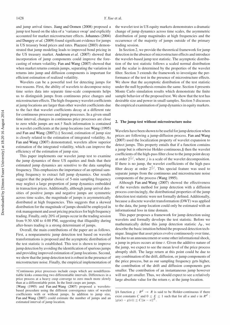
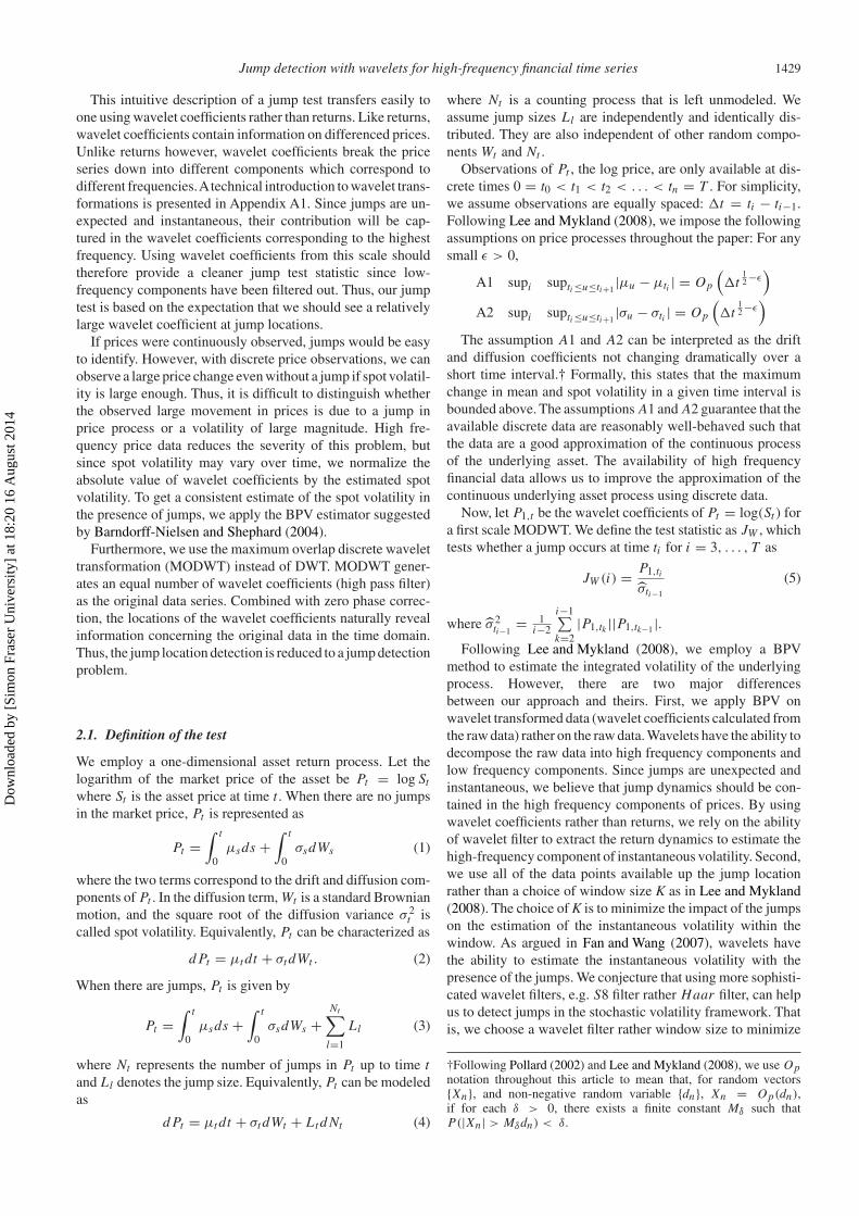
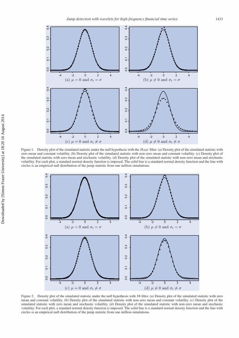
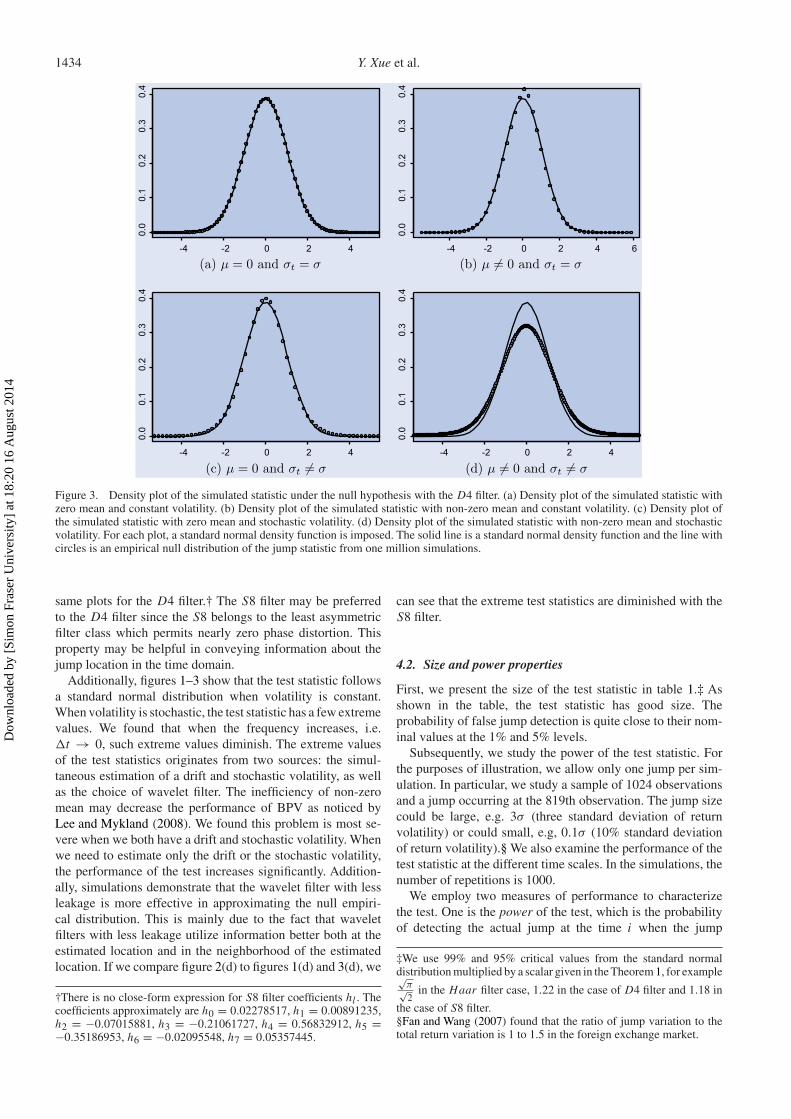
where k measures the recovery rate of volatility to the mean,log σ 2 is the long-run mean of variance, and δ is the diffusionparameter for the volatility process.‡ Following Fan and Wang(2007), we assume that the correlation between W1,t and W2,tis ρ, which is negative and captures the asymmetric impact ofthe innovation in price process. We set k = −0.1, log σ 2 =−6.802, and δ = 0.25. Figure 1 shows the density plot of thestatistic for 1 million observations when a Haar filter is used.The top left panel shows the zero mean and constant volatilitycase; the top right panel depicts the non-zero mean and constantvolatility case; the bottom left panel shows the zero mean andstochastic volatility case; and the bottom right panel depictsthe non-zero mean and stochastic volatility case.

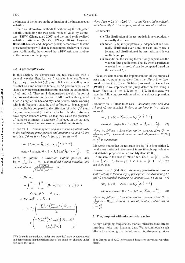
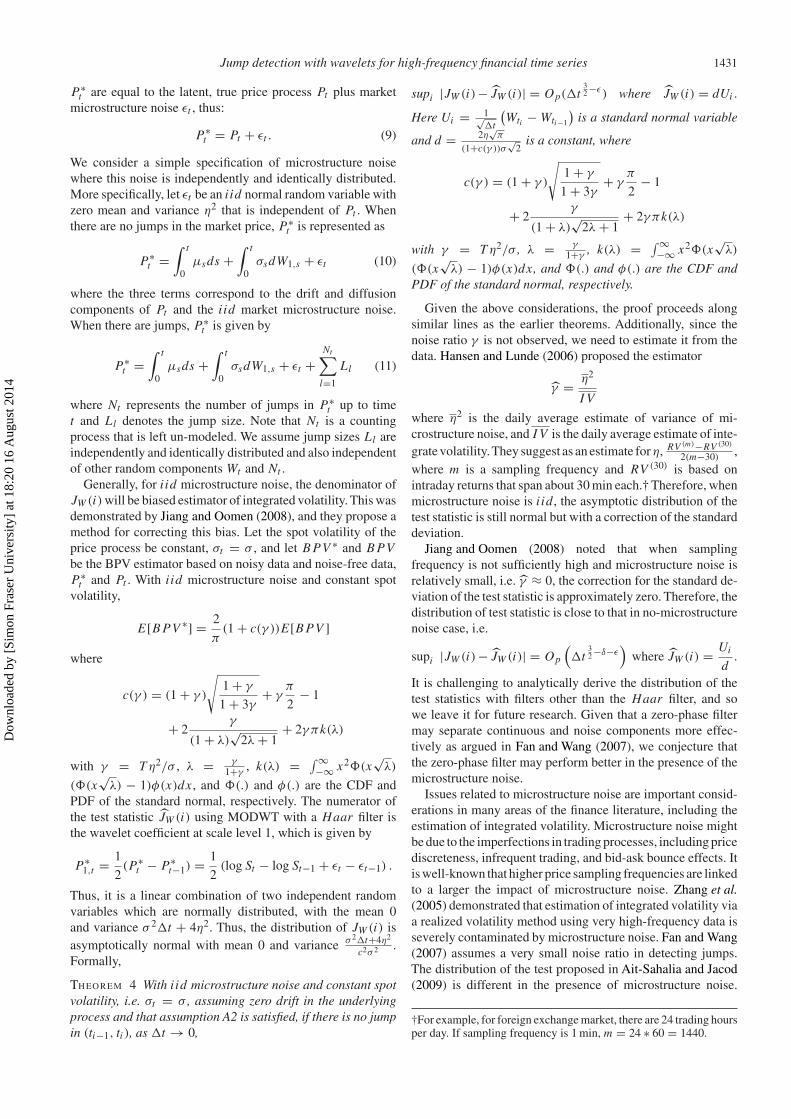
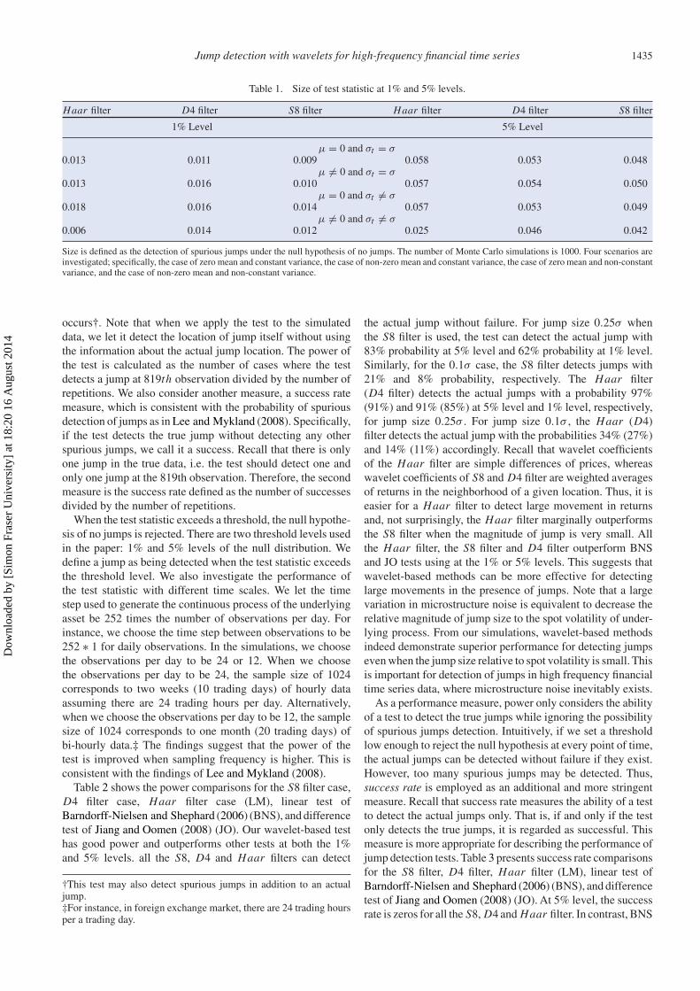
Figure 2 shows the density plot of the statistic for one millionobservations when an S8 filter is used, and figure 3 shows the

†We also investigated various specifications with drift and the driftpart has negligible impact on the main results.‡We also investigated other specifications of the process and foundthat different specifications of volatility processes did not qualitativelychanged the main results.

Dow

nloa

ded

by [

Sim

on F

rase

r U

nive

rsity

] at

18:

20 1

6 A

ugus

t 201

4

Jump detection with wavelets for high-frequency financial time series 1433

-4 -2 0 2 4

0.0

0.1

0.2

0.3

0.4

-4 -2 0 2 4

0.0

0.1

0.2

0.3

0.4

-4 -2 0 2 4

0.0

0.1

0.2

0.3

0.4

-4 -2 0 2 4

0.0

0.1

0.2

0.3

0.4

Figure 1. Density plot of the simulated statistic under the null hypothesis with the Haar filter. (a) Density plot of the simulated statistic withzero mean and constant volatility. (b) Density plot of the simulated statistic with non-zero mean and constant volatility. (c) Density plot ofthe simulated statistic with zero mean and stochastic volatility. (d) Density plot of the simulated statistic with non-zero mean and stochasticvolatility. For each plot, a standard normal density function is imposed. The solid line is a standard normal density function and the line withcircles is an empirical null distribution of the jump statistic from one million simulations.

-4 -2 0 2 4

0.0

0.1

0.2

0.3

0.4

-4 -2 0 2 4

0.0

0.1

0.2

0.3

0.4

-4 -2 0 2 4

0.0

0.1

0.2

0.3

0.4

-4 -2 0 2 4

0.0

0.1

0.2

0.3

0.4

Figure 2. Density plot of the simulated statistic under the null hypothesis with S8 filter. (a) Density plot of the simulated statistic with zeromean and constant volatility. (b) Density plot of the simulated statistic with non-zero mean and constant volatility. (c) Density plot of thesimulated statistic with zero mean and stochastic volatility. (d) Density plot of the simulated statistic with non-zero mean and stochasticvolatility. For each plot, a standard normal density function is imposed. The solid line is a standard normal density function and the line withcircles is an empirical null distribution of the jump statistic from one million simulations.

Dow

nloa

ded

by [

Sim

on F

rase

r U

nive

rsity

] at

18:

20 1

6 A

ugus

t 201

4

1434 Y. Xue et al.

-4 -2 0 2 4

0.0

0.1

0.2

0.3

0.4

-4 -2 0 2 4 6

0.0

0.1

0.2

0.3

0.4

-4 -2 0 2 4

0.0

0.1

0.2

0.3

0.4

-4 -2 0 2 4

0.0

0.1

0.2

0.3

0.4

Figure 3. Density plot of the simulated statistic under the null hypothesis with the D4 filter. (a) Density plot of the simulated statistic withzero mean and constant volatility. (b) Density plot of the simulated statistic with non-zero mean and constant volatility. (c) Density plot ofthe simulated statistic with zero mean and stochastic volatility. (d) Density plot of the simulated statistic with non-zero mean and stochasticvolatility. For each plot, a standard normal density function is imposed. The solid line is a standard normal density function and the line withcircles is an empirical null distribution of the jump statistic from one million simulations.

same plots for the D4 filter.† The S8 filter may be preferredto the D4 filter since the S8 belongs to the least asymmetricfilter class which permits nearly zero phase distortion. Thisproperty may be helpful in conveying information about thejump location in the time domain.

Additionally, figures 1–3 show that the test statistic followsa standard normal distribution when volatility is constant.When volatility is stochastic, the test statistic has a few extremevalues. We found that when the frequency increases, i.e.�t → 0, such extreme values diminish. The extreme valuesof the test statistics originates from two sources: the simul-taneous estimation of a drift and stochastic volatility, as wellas the choice of wavelet filter. The inefficiency of non-zeromean may decrease the performance of BPV as noticed byLee and Mykland (2008). We found this problem is most se-vere when we both have a drift and stochastic volatility. Whenwe need to estimate only the drift or the stochastic volatility,the performance of the test increases significantly. Addition-ally, simulations demonstrate that the wavelet filter with lessleakage is more effective in approximating the null empiri-cal distribution. This is mainly due to the fact that waveletfilters with less leakage utilize information better both at theestimated location and in the neighborhood of the estimatedlocation. If we compare figure 2(d) to figures 1(d) and 3(d), we

†There is no close-form expression for S8 filter coefficients hl . Thecoefficients approximately are h0 = 0.02278517, h1 = 0.00891235,h2 = −0.07015881, h3 = −0.21061727, h4 = 0.56832912, h5 =−0.35186953, h6 = −0.02095548, h7 = 0.05357445.

can see that the extreme test statistics are diminished with theS8 filter.

4.2. Size and power properties

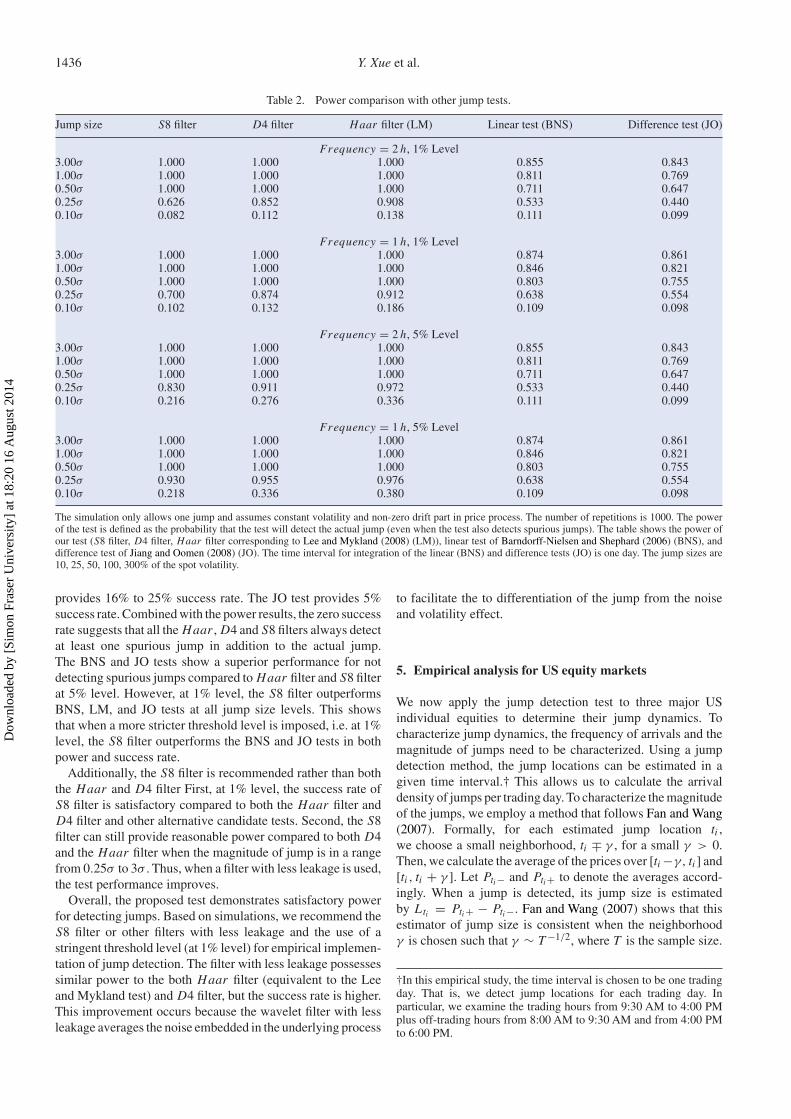
First, we present the size of the test statistic in table 1.‡ Asshown in the table, the test statistic has good size. Theprobability of false jump detection is quite close to their nom-inal values at the 1% and 5% levels.

Subsequently, we study the power of the test statistic. Forthe purposes of illustration, we allow only one jump per sim-ulation. In particular, we study a sample of 1024 observationsand a jump occurring at the 819th observation. The jump sizecould be large, e.g. 3σ (three standard deviation of returnvolatility) or could small, e.g, 0.1σ (10% standard deviationof return volatility).§ We also examine the performance of thetest statistic at the different time scales. In the simulations, thenumber of repetitions is 1000.

We employ two measures of performance to characterizethe test. One is the power of the test, which is the probabilityof detecting the actual jump at the time i when the jump

‡We use 99% and 95% critical values from the standard normaldistribution multiplied by a scalar given in the Theorem 1, for example√π√2

in the Haar filter case, 1.22 in the case of D4 filter and 1.18 in

the case of S8 filter.§Fan and Wang (2007) found that the ratio of jump variation to thetotal return variation is 1 to 1.5 in the foreign exchange market.

Dow

nloa

ded

by [

Sim

on F

rase

r U

nive

rsity

] at

18:

20 1

6 A

ugus

t 201

4

Jump detection with wavelets for high-frequency financial time series 1435

Table 1. Size of test statistic at 1% and 5% levels.

Haar filter D4 filter S8 filter Haar filter D4 filter S8 filter

1% Level 5% Level

μ = 0 and σt = σ0.013 0.011 0.009 0.058 0.053 0.048

μ = 0 and σt = σ0.013 0.016 0.010 0.057 0.054 0.050

μ = 0 and σt = σ0.018 0.016 0.014 0.057 0.053 0.049

μ = 0 and σt = σ0.006 0.014 0.012 0.025 0.046 0.042

Size is defined as the detection of spurious jumps under the null hypothesis of no jumps. The number of Monte Carlo simulations is 1000. Four scenarios areinvestigated; specifically, the case of zero mean and constant variance, the case of non-zero mean and constant variance, the case of zero mean and non-constantvariance, and the case of non-zero mean and non-constant variance.

occurs†. Note that when we apply the test to the simulateddata, we let it detect the location of jump itself without usingthe information about the actual jump location. The power ofthe test is calculated as the number of cases where the testdetects a jump at 819th observation divided by the number ofrepetitions. We also consider another measure, a success ratemeasure, which is consistent with the probability of spuriousdetection of jumps as in Lee and Mykland (2008). Specifically,if the test detects the true jump without detecting any otherspurious jumps, we call it a success. Recall that there is onlyone jump in the true data, i.e. the test should detect one andonly one jump at the 819th observation. Therefore, the secondmeasure is the success rate defined as the number of successesdivided by the number of repetitions.

When the test statistic exceeds a threshold, the null hypothe-sis of no jumps is rejected. There are two threshold levels usedin the paper: 1% and 5% levels of the null distribution. Wedefine a jump as being detected when the test statistic exceedsthe threshold level. We also investigate the performance ofthe test statistic with different time scales. We let the timestep used to generate the continuous process of the underlyingasset be 252 times the number of observations per day. Forinstance, we choose the time step between observations to be252 ∗ 1 for daily observations. In the simulations, we choosethe observations per day to be 24 or 12. When we choosethe observations per day to be 24, the sample size of 1024corresponds to two weeks (10 trading days) of hourly dataassuming there are 24 trading hours per day. Alternatively,when we choose the observations per day to be 12, the samplesize of 1024 corresponds to one month (20 trading days) ofbi-hourly data.‡ The findings suggest that the power of thetest is improved when sampling frequency is higher. This isconsistent with the findings of Lee and Mykland (2008).

Table 2 shows the power comparisons for the S8 filter case,D4 filter case, Haar filter case (LM), linear test ofBarndorff-Nielsen and Shephard (2006) (BNS), and differencetest of Jiang and Oomen (2008) (JO). Our wavelet-based testhas good power and outperforms other tests at both the 1%and 5% levels. all the S8, D4 and Haar filters can detect

†This test may also detect spurious jumps in addition to an actualjump.‡For instance, in foreign exchange market, there are 24 trading hoursper a trading day.

the actual jump without failure. For jump size 0.25σ whenthe S8 filter is used, the test can detect the actual jump with83% probability at 5% level and 62% probability at 1% level.Similarly, for the 0.1σ case, the S8 filter detects jumps with21% and 8% probability, respectively. The Haar filter(D4 filter) detects the actual jumps with a probability 97%(91%) and 91% (85%) at 5% level and 1% level, respectively,for jump size 0.25σ . For jump size 0.1σ , the Haar (D4)filter detects the actual jump with the probabilities 34% (27%)and 14% (11%) accordingly. Recall that wavelet coefficientsof the Haar filter are simple differences of prices, whereaswavelet coefficients of S8 and D4 filter are weighted averagesof returns in the neighborhood of a given location. Thus, it iseasier for a Haar filter to detect large movement in returnsand, not surprisingly, the Haar filter marginally outperformsthe S8 filter when the magnitude of jump is very small. Allthe Haar filter, the S8 filter and D4 filter outperform BNSand JO tests using at the 1% or 5% levels. This suggests thatwavelet-based methods can be more effective for detectinglarge movements in the presence of jumps. Note that a largevariation in microstructure noise is equivalent to decrease therelative magnitude of jump size to the spot volatility of under-lying process. From our simulations, wavelet-based methodsindeed demonstrate superior performance for detecting jumpseven when the jump size relative to spot volatility is small. Thisis important for detection of jumps in high frequency financialtime series data, where microstructure noise inevitably exists.

As a performance measure, power only considers the abilityof a test to detect the true jumps while ignoring the possibilityof spurious jumps detection. Intuitively, if we set a thresholdlow enough to reject the null hypothesis at every point of time,the actual jumps can be detected without failure if they exist.However, too many spurious jumps may be detected. Thus,success rate is employed as an additional and more stringentmeasure. Recall that success rate measures the ability of a testto detect the actual jumps only. That is, if and only if the testonly detects the true jumps, it is regarded as successful. Thismeasure is more appropriate for describing the performance ofjump detection tests. Table 3 presents success rate comparisonsfor the S8 filter, D4 filter, Haar filter (LM), linear test ofBarndorff-Nielsen and Shephard (2006) (BNS), and differencetest of Jiang and Oomen (2008) (JO). At 5% level, the successrate is zeros for all the S8, D4 and Haar filter. In contrast, BNS

Dow

nloa

ded

by [

Sim

on F

rase

r U

nive

rsity

] at

18:

20 1

6 A

ugus

t 201

4

1436 Y. Xue et al.

Table 2. Power comparison with other jump tests.

Jump size S8 filter D4 filter Haar filter (LM) Linear test (BNS) Difference test (JO)

Frequency = 2 h, 1% Level3.00σ 1.000 1.000 1.000 0.855 0.8431.00σ 1.000 1.000 1.000 0.811 0.7690.50σ 1.000 1.000 1.000 0.711 0.6470.25σ 0.626 0.852 0.908 0.533 0.4400.10σ 0.082 0.112 0.138 0.111 0.099

Frequency = 1 h, 1% Level3.00σ 1.000 1.000 1.000 0.874 0.8611.00σ 1.000 1.000 1.000 0.846 0.8210.50σ 1.000 1.000 1.000 0.803 0.7550.25σ 0.700 0.874 0.912 0.638 0.5540.10σ 0.102 0.132 0.186 0.109 0.098

Frequency = 2 h, 5% Level3.00σ 1.000 1.000 1.000 0.855 0.8431.00σ 1.000 1.000 1.000 0.811 0.7690.50σ 1.000 1.000 1.000 0.711 0.6470.25σ 0.830 0.911 0.972 0.533 0.4400.10σ 0.216 0.276 0.336 0.111 0.099

Frequency = 1 h, 5% Level3.00σ 1.000 1.000 1.000 0.874 0.8611.00σ 1.000 1.000 1.000 0.846 0.8210.50σ 1.000 1.000 1.000 0.803 0.7550.25σ 0.930 0.955 0.976 0.638 0.5540.10σ 0.218 0.336 0.380 0.109 0.098

The simulation only allows one jump and assumes constant volatility and non-zero drift part in price process. The number of repetitions is 1000. The powerof the test is defined as the probability that the test will detect the actual jump (even when the test also detects spurious jumps). The table shows the power ofour test (S8 filter, D4 filter, Haar filter corresponding to Lee and Mykland (2008) (LM)), linear test of Barndorff-Nielsen and Shephard (2006) (BNS), anddifference test of Jiang and Oomen (2008) (JO). The time interval for integration of the linear (BNS) and difference tests (JO) is one day. The jump sizes are10, 25, 50, 100, 300% of the spot volatility.

provides 16% to 25% success rate. The JO test provides 5%success rate. Combined with the power results, the zero successrate suggests that all the Haar , D4 and S8 filters always detectat least one spurious jump in addition to the actual jump.The BNS and JO tests show a superior performance for notdetecting spurious jumps compared to Haar filter and S8 filterat 5% level. However, at 1% level, the S8 filter outperformsBNS, LM, and JO tests at all jump size levels. This showsthat when a more stricter threshold level is imposed, i.e. at 1%level, the S8 filter outperforms the BNS and JO tests in bothpower and success rate.

Additionally, the S8 filter is recommended rather than boththe Haar and D4 filter First, at 1% level, the success rate ofS8 filter is satisfactory compared to both the Haar filter andD4 filter and other alternative candidate tests. Second, the S8filter can still provide reasonable power compared to both D4and the Haar filter when the magnitude of jump is in a rangefrom 0.25σ to 3σ . Thus, when a filter with less leakage is used,the test performance improves.

Overall, the proposed test demonstrates satisfactory powerfor detecting jumps. Based on simulations, we recommend theS8 filter or other filters with less leakage and the use of astringent threshold level (at 1% level) for empirical implemen-tation of jump detection. The filter with less leakage possessessimilar power to the both Haar filter (equivalent to the Leeand Mykland test) and D4 filter, but the success rate is higher.This improvement occurs because the wavelet filter with lessleakage averages the noise embedded in the underlying process

to facilitate the to differentiation of the jump from the noiseand volatility effect.

5. Empirical analysis for US equity markets

We now apply the jump detection test to three major USindividual equities to determine their jump dynamics. Tocharacterize jump dynamics, the frequency of arrivals and themagnitude of jumps need to be characterized. Using a jumpdetection method, the jump locations can be estimated in agiven time interval.† This allows us to calculate the arrivaldensity of jumps per trading day. To characterize the magnitudeof the jumps, we employ a method that follows Fan and Wang(2007). Formally, for each estimated jump location ti ,we choose a small neighborhood, ti ∓ γ , for a small γ > 0.Then, we calculate the average of the prices over [ti −γ, ti ] and[ti , ti + γ ]. Let Pti − and Pti + to denote the averages accord-ingly. When a jump is detected, its jump size is estimatedby Lti = Pti + − Pti −. Fan and Wang (2007) shows that thisestimator of jump size is consistent when the neighborhoodγ is chosen such that γ ∼ T −1/2, where T is the sample size.

†In this empirical study, the time interval is chosen to be one tradingday. That is, we detect jump locations for each trading day. Inparticular, we examine the trading hours from 9:30 AM to 4:00 PMplus off-trading hours from 8:00 AM to 9:30 AM and from 4:00 PMto 6:00 PM.

Dow

nloa

ded

by [

Sim

on F

rase

r U

nive

rsity

] at

18:

20 1

6 A

ugus

t 201

4

Jump detection with wavelets for high-frequency financial time series 1437

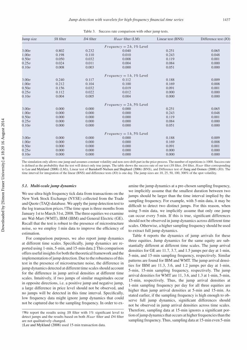
Table 3. Success rate comparison with other jump tests.

Jump size S8 filter D4 filter Haar filter (LM) Linear test (BNS) Difference test (JO)

Frequency = 2 h, 1% Level3.00σ 0.802 0.232 0.040 0.251 0.0651.00σ 0.198 0.110 0.010 0.243 0.0480.50σ 0.050 0.032 0.008 0.119 0.0010.25σ 0.024 0.011 0.004 0.084 0.0000.10σ 0.008 0.003 0.000 0.051 0.000

Frequency = 1 h, 1% Level3.00σ 0.240 0.117 0.112 0.188 0.0091.00σ 0.212 0.104 0.100 0.169 0.0080.50σ 0.156 0.032 0.019 0.091 0.0010.25σ 0.112 0.022 0.012 0.000 0.0000.10σ 0.004 0.005 0.004 0.000 0.000

Frequency = 2 h, 5% Level3.00σ 0.000 0.000 0.000 0.251 0.0651.00σ 0.000 0.000 0.000 0.243 0.0480.50σ 0.000 0.000 0.000 0.119 0.0010.25σ 0.000 0.000 0.000 0.084 0.0000.10σ 0.000 0.000 0.000 0.051 0.000

Frequency = 1 h, 5% Level3.00σ 0.000 0.000 0.000 0.188 0.0091.00σ 0.000 0.000 0.000 0.169 0.0080.50σ 0.000 0.000 0.000 0.091 0.0010.25σ 0.000 0.000 0.000 0.000 0.0000.10σ 0.000 0.000 0.000 0.000 0.000

The simulation only allows one jump and assumes constant volatility and non-zero drift part in the price process. The number of repetitions is 1000. Success rateis defined as the probability that the test will detect only true jumps. The table shows the success rate of our test (S8 filter, D4 filter, Haar filter correspondingto Lee and Mykland (2008) (LM)), Linear test of Barndorff-Nielsen and Shephard (2006) (BNS), and Difference test of Jiang and Oomen (2008) (JO). Thetime interval for integration of the linear (BNS) and difference tests (JO) is one day. The jump sizes are 10, 25, 50, 100, 300% of the spot volatility.

5.1. Multi-scale jump dynamics

We use ultra-high frequency tick data from transactions on theNew York Stock Exchange (NYSE) collected from the Tradeand Quote (TAQ) database. We apply the jump detection test tothe log transaction prices.†The time span is three months fromJanuary 1st to March 31st, 2008. The three equities we examineare Wal-Mart (WMT), IBM (IBM) and General Electric (GE).Recall that the test is robust to the presence of microstructurenoise, so we employ 1 min data to improve the efficiency ofestimation.

For comparison purposes, we also report jump dynamicsat different time scales. Specifically, jump dynamics are re-ported using 1-min, 5-min, and 15-min data.‡ This comparisonoffers useful insights for both the theoretical framework and theimplementation of jump detection. Due to the robustness of thistest in the presence of microstructure noise, the difference injump dynamics detected at different time scales should accountfor the difference in jump arrival densities at different timescales. Intuitively, if two jumps of similar magnitudes occurin opposite directions, i.e. a positive jump and negative jump,a large difference in price level should not be observed, andno jumps will be detected in this time interval. Specifically,low frequency data might ignore jump dynamics that couldnot be captured due to the sampling frequency. In order to ex-

†We report the results using S8 filter with 1% significant level todetect jumps and the results based on both Haar filter and D4 filterare not qualitatively changed.‡Lee and Mykland (2008) used 15-min transaction data.

amine the jump dynamics at a pre-chosen sampling frequency,we implicitly assume that the smallest duration between twojumps should be larger than the time interval implied by thesampling frequency. For example, with 5-min data, it may bedifficult to detect two distinct jumps. For this reason, whenusing 5-min data, we implicitly assume that only one jumpcan occur every 5 min. If this is true, significant differencesshould not be observed in jump dynamics across different timescales. Otherwise, a higher sampling frequency should be usedto extract full jump dynamics.

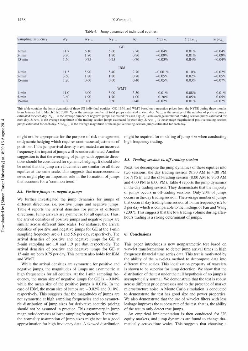
Table 4 reports the dynamics of jump arrivals for thesethree equities. Jump dynamics for the same equity are sub-stantially different at different time scales. The jump arrivaldensities for GE are 11.7, 3.7, and 1.5 jumps per day at 1-min,5-min, and 15-min sampling frequency, respectively. Similarpatterns are found for IBM and WMT. The jump arrival densi-ties for IBM are 11.3, 3.6, and 1.2 jumps per day at 1-min,5-min, 15-min sampling frequency, respectively. The jumparrival densities for WMT are 11, 3.6, and 1.3 at 1-min, 5-min,15-min, respectively. Thus, the jump arrival densities at1-min sampling frequency per day for all three equities arehigher than jump arrival densities at 5-min and 15-min. Asstated earlier, if the sampling frequency is high enough to ob-serve full jump dynamics, significant differences shouldnot be observed in jump arrival densities across time scales.Therefore, sampling data at 15-min ignores a significant por-tion of jump dynamics that occurs at higher frequencies than thesampling frequency. Thus, sampling data at 15-min even 5-min

Dow

nloa

ded

by [

Sim

on F

rase

r U

nive

rsity

] at

18:

20 1

6 A

ugus

t 201

4

1438 Y. Xue et al.

Table 4. Jump dynamics of individual equities.

Sampling frequency NT NT,+ NT,− Nt Si zeNt Si zeNt,+ SizeNt,−

GE1-min 11.7 6.10 5.60 2.70 −0.04% 0.01% −0.04%5-min 3.70 1.80 1.90 0.90 −0.09% 0.01% −0.09%15-min 1.50 0.75 0.75 0.70 −0.03% 0.04% −0.04%

IBM1-min 11.3 5.90 5.40 2.70 −0.001% 0.10% −0.02%5-min 3.60 1.80 1.80 0.70 −0.05% 0.02% −0.05%15-min 1.20 0.60 0.60 0.40 −0.05% 0.03% −0.07%

WMT1-min 11.0 6.00 5.00 3.50 −0.01% 0.08% −0.01%5-min 3.60 1.90 1.70 1.00 −0.20% 0.05% −0.05%15-min 1.30 0.80 0.50 0.40 −0.02% 0.01% −0.02%

This table contains the jump dynamics of three US individual equities: GE, IBM, and WMT based on transaction prices from the NYSE during three monthsfrom January 1st to March 31st, 2008. NT is the average number of total jumps estimated in each day. NT,+ is the average of the number of positive jumpsestimated for each day. NT,− is the average number of negative jumps estimated for each day. Nt is the average number of trading session jumps estimated foreach day. SizeNt is the average magnitude of the trading-session jumps estimated for each day. SizeNt,+ is the average magnitude of positive trading-sessionjumps estimated for each day. SizeNt,− is the average magnitude of the negative trading-session jumps estimated for each day.

might not be appropriate for the purpose of risk managementor dynamic hedging which requires continuous adjustments ofpositions. If the jump arrival density is estimated at an incorrectfrequency, the impact of jumps will be underestimated.Anothersuggestion is that the averaging of jumps with opposite direc-tions should be considered for dynamic hedging. It should alsobe noted that the jump arrival densities are similar for all threeequities at the same scale. This suggests that macroeconomicnews might play an important role in the formation of jumpsthat accounts for a ‘common trend.’

5.2. Positive jumps vs. negative jumps

We further investigated the jump dynamics for jumps ofdifferent directions, i.e. positive jumps and negative jumps.Table 4 reports the arrival densities for jumps of differentdirections. Jump arrivals are symmetric for all equities. Thus,the arrival densities of positive jumps and negative jumps aresimilar across different time scales. For instance, the arrivaldensities of positive and negative jumps for GE at the 1-minsampling frequency are 6.1 and 5.6 per day, respectively. Thearrival densities of positive and negative jumps for GE at5-min sampling are 1.8 and 1.9 per day, respectively. Thearrival densities of positive and negative jumps for GE at15-min are both 0.75 per day. This pattern also holds for IBMand WMT.

While the arrival densities are symmetric for positive andnegative jumps, the magnitudes of jumps are asymmetric athigh frequencies for all equities. At the 1-min sampling fre-quency, the mean size of negative jumps for GE is −0.04%while the mean size of the positive jumps is 0.01%. In thecase of IBM, the mean size of jumps are −0.02% and 0.10%,respectively. This suggests that the magnitudes of jumps arenot symmetric at high sampling frequencies and so symmet-ric distribution of jump sizes for derivative security pricingshould not be assumed in practice. This asymmetry in jumpmagnitude decreases at lower sampling frequencies. Therefore,the normality assumption of jump sizes might not be a goodapproximation for high frequency data. A skewed distribution

might be required for modeling of jump size when conductinghigh frequency trading.

5.3. Trading session vs. off-trading session

Next, we decompose the jump dynamics of these equities intotwo sessions: the day trading session (9:30 AM to 4:00 PMfor NYSE) and the off-trading session (8:00 AM to 9:30 AMand 4:00 PM to 6:00 PM). Table 4 reports the jump dynamicsin the day trading session. They demonstrate that the majorityof jumps occurs in off-trading sessions. Only 20% of jumpsoccurs in the day trading session. The average number of jumpsthat occur in day trading time session at 1-min frequency is 2 to3 per day which is comparable to the findings of Fan and Wang(2007). This suggests that the low trading volume during after-hours trading is a strong determinant of jumps.

6. Conclusions

This paper introduces a new nonparametric test based onwavelet transformations to detect jump arrival times in highfrequency financial time series data. This test is motivated bythe ability of the wavelets method to decompose data intodifferent time scales. This localization property of waveletsis shown to be superior for jump detection. We show that thedistribution of the test under the null hypothesis of no jumps isasymptotically normal. We demonstrate that the test is robustacross different price processes and to the presence of marketmicrostructure noise. A Monte Carlo simulation is conductedto demonstrate the test has good size and power properties.We also demonstrate that the use of wavelet filters with lessleakage improves the success rate of the test, that is, the abilityof the test to only detect true jumps.

An empirical implementation is then conducted for USequity markets, and jump dynamics are found to change dra-matically across time scales. This suggests that choosing a

Dow

nloa

ded

by [

Sim

on F

rase

r U

nive

rsity

] at

18:

20 1

6 A

ugus

t 201

4

Jump detection with wavelets for high-frequency financial time series 1439

proper sampling frequency is very important for investigatingjump dynamics. Additionally, the arrival densities of positivejumps and negative jumps are similar, but the magnitudes ofthe jumps are asymmetrically distributed at high frequencies.Finally, the majority of jumps occur outside of the day tradingsession with only 20% of jumps occuring within these sessions.

Acknowledgements

Yi Xue gratefully acknowledge financial support from theNational Natural Science Foundation of China (NSFC), projectNo. 71101031. Ramazan Gençay gratefully acknowledgesfinancial support from the Natural Sciences and EngineeringResearch Council of Canada and the Social Sciences and Hu-manities Research Council of Canada. This paper is supportedby Program for Innovative Research Team in UIBE. We wouldlike to thank two referees for their helpful comments and valu-able suggestions which have improved the paper greatly. Theremaining errors are ours.

References

Ait-Sahalia,Y. and Jacod, J., Testing for jumps in a discretely observedprocess. Ann. Stat., 2009, 37, 184–222.

Andersen, T., Bollerslev, T., Diebold, F. and Labys, P., Modeling andforecasting realized volatility. Econometrica, 2003, 71, 579–625.

Andersen, T., Bollerslev, T. and Diebold, F., Roughing it up: Includingjump components in the measurement modeling and forecasting ofreturn volatility. Rev. Econ. Stat., 2007, 89, 701–720.

Barndorff-Nielsen, O.E. and Shephard, N., Power and bipowervariation with stochastic volatility and jumps. J. Financ. Econom.,2004, 2, 1–37.

Barndorff-Nielsen, O.E. and Shephard, N., Economettrics of testingfor jumps in financial economics using bipower variation. J.Financ. Econom., 2006, 4, 1–30.

Daubechies, I., Orthonormal bases of compactly supported wavelets.Comm. Pure Appl. Math., 1988, 41, 909–996.

Dungey, M., McKenzie, M. and Smith, V., Empirical evidence onjumps in the term structure of the US treasury market. J. Empir.Finance, 2009, 16, 430–445.

Fan, J. and Wang,Y., Multi-scale jump and volatility analysis for high-frequency financial data. J. Am. Stat. Assoc., 2007, 102, 1349–1362.

Gençay, R., Selçuk, F. and Whitcher, B., An Introduction to Waveletsand Other Filtering Methods in Finance and Economics, 2001(Academic Press: New York).

Haar, A., Zur theorie der orthogonalen funktionensysteme. Math.Ann., 1910, 69, 331–371.

Hansen, P.R. and Lunde, A., Realized variance and marketmicrostructure noise. J. Bus. Econ. Stat., 2006, 24, 127–161.

Jacod, J., Li, Y., Mykland, P.A., Podolskij, M. and Vetter, M.,Microstructure noise in the continuous case: The pre-averagingapproach. Stoch. Process. Appl., 2009, 119, 2249–2276.

Jiang, G.J. and Oomen, R.C., Testing for jumps when asset prices areobserved with noise – a swap variance approach. J. Econom., 2008,144, 352–370.

Johannes, M., The statistical and economic role of jumps incontinuous-time interest rate models. J. Finance, 2004, 59, 227–260.

Lee, S.S. and Mykland, P.A., Jumps in financial markets: A newnonparametric test and jump dynamics. Rev. Financ. Stud., 2008,21, 2535–2563.

Leone, F.C., Nelson, L.S. and Nottingham, R.B., The folded normaldistribution. Technometrics, 1961, 3, 543–550.

Piazzesi, M., Bond yields and the federal reserve. J. Polit. Econ.,2003, 113, 311–344.

Podolskij, M. and Vetter, M., Estimation of volatility functionalsin the simultaneous presence of microstructure noise and jumps.Bernoulli, 2009, 315, 634–658.

Pollard, D., A User’s Guide of Measure Theoretic Probability, 2002(Cambridge University Press: Cambridge).

Protter, P., Stochastic Integration and Differential Equations: A NewApproach, 2004 (Springer: New York).

Wang, Y., Jump and sharp cusp detection by wavelets. Biometrika,1995, 82, 385–397.

Zhang, L., Efficient estimation of stochastic volatility using noisyobservations: A multi-scale approach. Working Paper, CarnegieMellon University, 2006.

Zhang, L., Ait-Sahalia, Y. and Mykland, A., A tale of two time scales:Determining integrated volatility with noisy high-frequency data.J. Am. Stat. Assoc., 2005, 100, 1394–1411.

Appendix A1. Wavelet Transformations†

A wavelet is a small wave which grows and decays in a lim-ited time period.‡ To formalize the notion of a wavelet, letψ(.) be a real valued function such that its integral is zero,∫∞−∞ ψ(t) dt = 0, and its square integrates to unity,

∫∞−∞ ψ(t)2

dt = 1. Thus, althoughψ(.)has to make some excursions awayfrom zero, any excursions it makes above zero must cancel outexcursions below zero, i.e. ψ(.) is a small wave, or a wavelet.

Fundamental properties of the continuous wavelet functions(filters), such as integration to zero and unit energy, havediscrete counterparts. Let h = (h0, . . . , hL−1) be a finitelength discrete wavelet (or high pass) filter such that it in-tegrates (sums) to zero,

∑L−1l=0 hl = 0, and has unit energy,∑L−1

l=0 h2l = 1. In addition, the wavelet filter h is orthogonal to

its even shifts; that is,

L−1∑l=0

hlhl+2n =∞∑

l=−∞hlhl+2n = 0, for all nonzero integers n.

(15)The natural object to complement a high-pass filter is a low-

pass (scaling) filter g. We will denote a low-pass filter asg = (g0, . . . , gL−1). The low-pass filter coefficients are de-termined by the quadrature mirror relationship§

gl = (−1)l+1hL−1−l for l = 0, . . . , L − 1 (16)

and the inverse relationship is given by hl = (−1)l gL−1−l .The basic properties of the scaling filter are:

∑L−1l=0 gl = √

2,∑L−1l=0 g2

l = 1,

L−1∑l=0

gl gl+2n =∞∑

l=−∞gl gl+2n = 0, (17)

for all nonzero integers n, and

L−1∑l=0

glhl+2n =∞∑

l=−∞glhl+2n = 0 (18)

†This appendix offers a brief introduction to Wavelet transformations.Interested readers can consult Gençay et al. (2001) for more details.‡This section closely follows Gençay et al. (2001). The contrastingnotion is a big wave such as the sine function which keeps oscillatingindefinitely.§Quadrature mirror filters (QMFs) are often used in the engineeringliterature because of their ability for perfect reconstruction of a signalwithout aliasing effects. Aliasing occurs when a continuous signal issampled to obtain a discrete time series.

Dow

nloa

ded

by [

Sim

on F

rase

r U

nive

rsity

] at

18:

20 1

6 A

ugus

t 201

4

1440 Y. Xue et al.

for all integers n. Thus, scaling filters are average filters andtheir coefficients satisfy the orthonormality property that theypossess unit energy and are orthogonal to even shifts. By ap-plying both h and g to an observed time series, we can sep-arate high-frequency oscillations from low-frequency ones.In the following sections, we will briefly describe DWT andMODWT.

A1.1 Discrete wavelet transformation

With both wavelet filter coefficients and scaling filter coeffi-cients, we can decompose the data using the (discrete) wavelettransformation (DWT). Formally, let us introduce the DWTthrough a simple matrix operation. Let y to be the dyadiclength vector (T = 2J ) of observations. The length T vectorof discrete wavelet coefficients w is obtained via

w = Wy

where W is an T × T orthonormal matrix defining the DWT.The vector of wavelet coefficients can be organized intoJ +1 vectors, w = [w1,w2, . . . ,wJ , vJ ]′ , where w j is a lengthT/2 j vector of wavelet coefficients associated with changes ona scale of length λ j = 2 j−1, and vJ is a length T/2J vectorof scaling coefficients associated with averages on a scale oflength 2J = 2λJ .

The matrix W is composed of the wavelet and scaling filtercoefficients arranged on a row-by-row basis. Let

h1 = [h1,N−1, h1,N−2, . . . , h1,1, h1,0]′

be the vector of zero-padded unit scale wavelet filter coeffi-cients in reverse order. Thus, the coefficients h1,0, . . . , h1,L−1are taken from an appropriate ortho-normal wavelet family oflength L , and all values L < t < T are defined to be zero.Now circularly shift h1 by factors of two so that

h(2)1 = [h1,1, h1,0, h1,N−1, h1,N−2 . . . , h1,3, h1,2]′

h(4)1 = [h1,3, h1,2, h1,1, h1,0 . . . , h1,5, h1,4]′

and so on. Define the T/2 × T dimensional matrix W1 to bethe collection of T/2 circularly shifted versions of h1. Hence,

W1 = [h(2)1 ,h(4)1 , . . . ,h(T/2−1)1 ,h1]′

Let h2 be the vector of zero-padded scale 2 wavelet filtercoefficients defined similarly to h1. W2 is constructed by cir-cularly shifting the vector h2 by factor of four. Repeat this toconstruct W j by circularly shifting the vector h j (the vectorof zero-padded scale j wavelet filter coefficients) by 2 j . Thematrix VJ is simply a column vector whose elements are allequal to 1/

√T . Then, the T × T dimensional matrix W is

W = [W1,W2, . . . ,WJ ,VJ ]′ .When we are provided with a dyadic length time series, it

is not necessary to implement the DWT down to level J =log2(T ). A partial DWT may be performed instead that ter-minates at level Jp < J . The resulting vector of waveletcoefficients will now contain T − T/2Jp wavelet coefficientsand T/2Jp scaling coefficients.

The orthonormality of the matrix W implies that the DWTis a variance preserving transformation:

‖w‖2 =T/2J∑t=1

v2t,J +

J∑j=1

⎛⎝T/2 j∑t=1

w2t, j

⎞⎠ =T∑

t=1

y2t = ‖y‖2 .

This can be easily proven through basic matrix manipulationvia

‖y‖2 = y′y = (W−1w)

′W−1w = w′(WW ′

)−1w

= w′w = ‖w‖2 .

The first equality holds because of definition of ‖y‖2. Thesecond equality holds because that given w = Wy, we havey = W−1w. Therefore, substituting y = W−1w into y

′y leads

to the second equality. The third equality holds because of theproperties of matrix inversion and transposition. The fourthequality holds the property of orthonormal matrix. Notice thatsince W is orthonormal matrix, we have W−1 = W ′

. Thus,WW ′ = WW−1 = I , where I is identity matrix.

Given the structure of the wavelet coefficients, ‖y‖2 is de-composed on a scale-by-scale basis via

‖y‖2 =J∑

j=1

∥∥w j∥∥2 + ‖vJ ‖2 (19)

where∥∥w j

∥∥2 =∑T/2 j

t=1 w2t, j is the sum of squared variation of

y due to changes at scale λ j and ‖vJ ‖2 = ∑T/2J

t=1 v2t,J is the

information due to changes at scales λJ and higher.

A1.2 Maximum overlap discrete wavelet transformation

An alternative wavelet transform is MODWT which is com-puted by not subsampling the filtered output. Let y be anarbitrary length T vector of observations. The length (J +1)Tvector of MODWT coefficients w is obtained via

w = Wy,

where W is a (J +1)T × T matrix defining the MODWT. Thevector of MODWT coefficients may be organized into J + 1vectors via

w = [w1, w2, . . . , wJ , vJ ]T , (20)

where w j is a length T vector of wavelet coefficients associatedwith changes on a scale of length λ j = 2 j−1 and vJ is a lengthT vector of scaling coefficients associated with averages on ascale of length 2J = 2λJ , just as with the DWT.

Similar to the orthonormal matrix defining the DWT, thematrix W is also made up of J + 1 submatrices, each of themT × T , and may be expressed as

W =

⎡⎢⎢⎢⎢⎢⎣W1

W2...

WJ

VJ

⎤⎥⎥⎥⎥⎥⎦ .The MODWT utilizes the rescaled filters ( j = 1, . . . , J )

h j = h j/2j/2 and gJ = gJ/2

J/2.

To construct the T × T dimensional submatrix W1, we circu-larly shift the rescaled wavelet filter vector h1 by integer unitsto the right so that

Dow

nloa

ded

by [

Sim

on F

rase

r U

nive

rsity

] at

18:

20 1

6 A

ugus

t 201

4

Jump detection with wavelets for high-frequency financial time series 1441

W1 =[h(1)1 , h(2)1 , h(3)1 , . . . , h(N−2)

1 , h(N−1)1 , h1

]T. (21)

This matrix may be interpreted as the interweaving of the DWTsubmatrix W1 with a circularly shifted (to the right by one unit)version of itself. The remaining submatrices W2, . . . , WJ areformed similarly to equation (21), only replace h1 by h j .

In practice, a pyramid algorithm is utilized similar to that ofthe DWT to compute the MODWT. Starting with the data xt

(no longer restricted to be a dyadic length), filter it using h1and g1 to obtain the length T vectors of wavelet and scalingcoefficients w1 and v1, respectively.

For each iteration of the MODWT pyramid algorithm, werequire three objects: the data vector x, the wavelet filter hl andthe scaling filter gl . The first iteration of the pyramid algorithmbegins by filtering (convolving) the data with each filter toobtain the following wavelet and scaling coefficients:

w1,t =L−1∑l=0

hl yt−l mod T and v1,t =L−1∑l=0

gl yt−l mod T ,

where t = 1, . . . , T . The length T vector of observations hasbeen high- and low-pass filtered to obtain T coefficients asso-ciated with this information. The second step of the MODWTpyramid algorithm starts by defining the data to be the scalingcoefficients v1 from the first iteration and apply the filteringoperations as above to obtain the second level of wavelet andscaling coefficients

w2,t =L−1∑l=0

hl v1,t−2l mod T and v2,t =L−1∑l=0

gl v1,t−2l mod T ,

t = 1, . . . , T . Keeping all vectors of wavelet coefficients,and the final level of scaling coefficients, we have the fol-lowing length T decomposition: w = [w1 w2 v2]′ . After thethird iteration of the pyramid algorithm, where we apply filter-ing operations to v2, the decomposition now looks like w =[w1 w2 w3 v3]′ . This procedure may be repeated up to Jtimes where J = log2(T ) and gives the vector of MODWTcoefficients in equation (20).

Similar to DWT, MODWT wavelet and scaling coefficientsare variance preserving

‖w‖2 =T∑

t=1

v2t,J +

J∑j=1

(T∑

t=1

w2t, j

)=

T∑t=1

y2t = ‖y‖2 .

and a partial decomposition Jp < J may be performed whenit deems necessary.

The following properties are important for distinguishingthe MODWT from the DWT. The MODWT can accommodateany sample size T , while the Jpth order partial DWT restrictsthe sample size to a multiple of 2Jp . The detail and smoothcoefficients of a MODWTare associated with zero phase filters.Thus, events that feature in the original time series can beproperly aligned with features in the MODWT multiresolutionanalysis. The MODWT is invariant to circular shifts in theoriginal time series. This property does not hold for the DWT.The MODWT wavelet variance estimator is asymptoticallymore efficient than the same estimator based on the DWT.For both MODWT and DWT, the scaling coefficients containthe lowest frequency information. But each level’s wavelet

coefficients contain progressively lower frequency informa-tion.

Appendix A2. Proofs of Theorems

Theorem 1 Assuming zero drift and constant spot volatilityin the underlying price process and assuming A1 and A2 aresatisfied, if there is no jump in (ti−1, ti ), as �t → 0

supi |JW (i)− JW (i)| = Op(�t32 −δ−ε),

where δ satisfies 0 < δ < 3/2 and JW (i) = Ui

d. (22)

where Wt follows a Brownian motion process. AndUi = 1√

�t(Wti − Wti−1), a standard normal variable, and

a constant d =√

E[B PVG ]√∑L−2l=0 (

∑lj=0 h j )

2, where

E[B PVG]=∫ ∞

−∞. . .

∫ ∞

−∞E[B PVG |x1, . . . , xL−2]φ(x1)

. . . φ(xL−2)dx1 . . . dxL−2,

E[B PVG |r1, . . . , rL−2]

= 2σ 2 f

⎛⎝−∑L−2l=1

(∑lj=0 h j

)(rL−l−l)

h0

⎞⎠× f

⎛⎝−∑L−3l=0

(∑lj=0 h j

)(rL−l−l)(∑L−2

j=0 h j

)⎞⎠ ,

where f (a) = 2φ(a)+2a�(a)−a, and rt s are independentlyand identically distributed (iid) standard normal variables.

Proof Assuming zero drift, using MODWT with a generalfilter to transform the data, the wavelet coefficients at scale 1are

P1,ti =L−1∑l=0

hl(Pti−l − Pti−l−1). (23)

Since∑L−1

l=0 hl = 0, we have hL−1 = −∑L−2l=0 hl . Therefore,

equation (23) can be rewritten as

P1,ti =L−2∑l=0

⎛⎝ l∑j=0

h j

⎞⎠(Pti−l − Pti−l−1

). (24)

Hence we have

Pti−l − Pti−l−1 = log Sti −l − log Sti−l−1

=∫ ti−l

ti−l−1

μudu +∫ ti−l

ti−l−1

σudW (u). (25)

Imposing assumption A1, we have∫ ti

ti−1

μudu − μti−1�t = Op

(�t

32 −ε) (26)

This implies

sup|∫ ti

ti−1

[μu − μu−1]du| = Op

(�t

32 −ε) (27)

Dow

nloa

ded

by [

Sim

on F

rase

r U

nive

rsity

] at

18:

20 1

6 A

ugus

t 201

4

1442 Y. Xue et al.

Similarly, applying Burkholder’s inequality (Protter 2004),†we have

sup|∫ ti

ti−1

[σu − σu−1]dW (u)| = Op

(�t

32 −δ−ε) (28)

where δ can be any number in 0 < δ < 3/2. Therefore overthe window, for t ∈ [ti−1, ti ], d log St can be approximated byd log Si

t , such that

d log Sit = μti−1dt + σti−1dW (t) (29)

because

|(log Sti − log Sti−1)− (log Siti − log Si

ti−1)|

= |∫ ti

ti−1

(μu − μti−1

)du +

∫ ti

ti−1

(σu − σti−1

)dW (u)|

= OP

(�t

32 −δ−ε) (30)

Therefore, for all i, j and t j ∈ [ti−1, ti ], the numerator is

log St j − log St j−1 = log Sit j

− log Sit j−1

+ OP

(�t

32 −δ−ε)

= σti−1 W�t + OP

(�t

32 −δ−ε)

= σti−1

√�tUi + Op

(�t

32 −δ−ε) (31)

where W�t = Wti − Wti−1 , Ui = 1√�t(Wti − Wti−1), which is

an independently identically distributed (i id) normal.Hence, P1,ti is a linear combination of i id normal variables

Ui s. Therefore, P1,ti is normally distributed with mean 0 andvariance

σP,ti =

√√√√√L−2∑l=0

⎛⎝ l∑j=0

h j

⎞⎠2

σ 2ti−l−1

�t (32)

And it is σ

√∑L−2l=0

(∑lj=0 h j

)2�t if σt = σ . Formally,

P1,ti =

⎛⎜⎜⎝√√√√√L−2∑

l=0

⎛⎝ l∑j=0

h j

⎞⎠2⎞⎟⎟⎠ σ√

�tUi + Op

(�t

32 −δ−ε)

where Ui = 1√∑L−2l=0

(∑lj=0 h j

)2

∑L−2l=0

(∑lj=0 h j

)(Ui−l),

which is standard normal but not independent anymore.For the denominator, notice that increment of the numer-

ator is not independent anymore, i.e. a direct application ofBarndorff-Nielsen and Shephard (2004) is not applicable. Forexpositional purpose, let rL−l−1 = log Sti−l − log Sti−l−1 andrL−l−1 = rL−l−1

σ�t ∼ i id N(0,1). Consequently, we have:

†This inequality gives bounds for the maximum of a martingale interms of the quadratic variation. For a local martingale M startingat zero, with maximum denoted by M∗

t = sups≤t |Ms |, and for any

real number p ≥ 1, the inequality is cp E([M]p2t ) ≤ E((M∗

t )p) ≤

C p E([M]p2t ), where cp ≤ C p are constant depending on the choice

of p, but not depending on the martingale M and t used. If M iscontinuous martingale, then this inequality holds for any p.

E[B PVG ]

= σ 2 E |L−2∑l=0

⎛⎝ l∑j=0

h j

⎞⎠ (rL−l−1) ||L−2∑l=0

⎛⎝ l∑j=0

h j

⎞⎠ (rL−l−2) |

Conditional on r1, . . ., rL−2 and we can get‡

E[B PVG |r1, . . . , rL−2]

= 2σ 2 f

(−∑L−2l=1 (

∑lj=0 h j )(rL−l−1)

h0

)

× f

(−∑L−3l=0 (

∑lj=0 h j )(rL−l−1)

(∑L−2

j=0 h j )

)with

f (a) = 2φ(a)+ 2a�(a)− a

where a is a constant, x ∼ i id N(0,1) and φ(.) and�(.) denotethe PDF and CDF of a standard normal. Notice that r1, . . ., rL−2are i id standard normals, Thus,

E[B PVG]=∫ ∞

−∞. . .

∫ ∞

−∞E[B PVG |r1, . . . , rL−2]φ(r1)

. . . φ(rL−2)dr1 . . . drL−2

That is,

JW (i) =σ

√∑L−2l=0 (

∑lj=0 h j )2

σ√

E[B PVG] Ui + Op

(�t

32 −δ−ε)

Let d =√

E[B PVG ]√∑L−2l=0 (

∑lj=0 h j )

2, we have

= Ui

d+ Op

(�t

32 −δ−ε) .

�Proposition 2 (Haar filter case) Assuming zero drift andA1 and A2 are satisfied. If there is no jump in (ti−1, ti ), as�t → 0,

supi |JW (i)− JW (i)| = Op(�t32 −δ−ε),

where δ satisfies 0 < δ < 3/2 and JW (i) = Ui

d. (33)

where Wt follows a Brownian motion process. HereUi = 1√

�t(Wti − Wti−1), a standard normal variable, and

d = E[|Ui |] =√

2√π

is a constant.

Proof This proof follows a similar line of reasoning toTheorem 1 and 1.1 in Lee and Mykland (2008). Using MODWTwith the Haar filter to transform the data, the wavelet coeffi-cients at scale level 1 are

P1,ti = 1

2

(Pti − Pti−1

) = 1

2

(log Sti − log Sti−1

). (34)

That is, our test statistic is of the form

JW (i) =12 (log Sti − log Sti−1)

12 σti−1

(35)

‡Given a normally distributed random variable X with mean μ andvariance σ 2, the random variable Y = |X | has a folded normaldistribution. For further reference, please see Leone et al. (1961).

Dow

nloa

ded

by [

Sim

on F

rase

r U

nive

rsity

] at

18:

20 1

6 A

ugus

t 201

4

Jump detection with wavelets for high-frequency financial time series 1443

which is equivalent to the Lee and Mykland (2008) test withthe window size of one data point prior to the location to bedetected. The numerator, under the no-drift assumption, is

log Sti − log Sti−1 =∫ ti

ti−1

σudW (u). (36)

Applying Burkholder’s inequality (Protter 2004), we have

sup|∫ ti

ti−1

[σu − σu−1]dW (u)| = Op

(�t

32 −δ−ε) (37)

where δ can be any number in 0 < δ < 3/2. Therefore, fort ∈ [ti−1, ti ], d log St can be approximated by d log Si

t , suchthat

d log Sit = σti−1dW (t) (38)

because

|(log Sti − log Sti−1)− (log Siti − log Si

ti−1)|

=∣∣∣∣∫ ti

ti−1

(σu − σti−1)dW (u)

∣∣∣∣= OP

(�t

32 −δ−ε) . (39)

Therefore, for all i, j and t j ∈ [ti−1, ti ], the numerator of thetest statistic is

log St j − log St j−1 = log Sit j

− log Sit j−1

+ OP

(�t

32 −δ−ε)

= σti−1 W�t + OP

(�t

32 −δ−ε)

= σti−1

√�tUi + Op

(�t

32 −δ−ε) (40)

where W�t = Wti −Wti−1 , Ui = 1√�t(Wti −Wti−1), which is an

independently identically distributed normal random variable.Notice the second equality follows directly from equation (38)and third equality follows directly from our definition. For thedenominator,

1

i − 2

i−1∑k=2

|P1,tk ||P1,tk−1 |

= 1

4

1

(i − 2)

i−1∑k=2

| log Stk − log Stk−1 || log Stk−1 − log Stk−2 |(41)

Following Barndorff-Nielsen and Shephard (2004), we have

plim�t→0c2σ 2ti−1

= plim�t→01

(i − 2)�t

i−1∑k=2

| log Stk − log Stk−1 || log Stk−1 − log Stk−2 |= d2σ 2

ti−1(42)

where d = E[|Ui |] =√

2√π

. Hence

plim�t→01

(i − 2)�t

i−1∑k=2

|P1,tk ||P1,tk−1 | = 1

4d2σ 2

ti−1(43)

Therefore, the test statistics is

JW (i) = Ui

d+ Op(�t

32 −δ−ε). (44)

�

Proposition 3 (D4 filter) Assuming zero drift and constantspot volatility in the underlying price process and assuming A1and A2 are satisfied, if there is no jump in (ti−1, ti ), as�t → 0

supi |JW (i)− JW (i)| = Op

(�t

32 −δ−ε) ,

where δ satisfies 0 < δ < 3/2 and JW (i) = Ui

d. (45)

where Wt follows a Brownian motion process. Here Ui =1√�t(Wti − Wti−1), a standard normal variable, and a constant

d ≈√

2√3

.

Proof Assuming zero drift and using MODWT with the D(4)filter to transform the data, the wavelet coefficients at scale 1are

P1,ti = 1

8((1 − √

3)Pti + (√

3 − 3)Pti−1 + (3 + √3)Pti−2

+ (−1 − √3)Pti−3)

= 1

8((1 − √

3)(Pti − Pti−1)+ (1 + √3)(Pti−2 − Pti−3)

− 2(Pti−1 − Pti−2))

= 1

8((1 − √

3)(log Sti − log Sti−1)+ (1 + √3)

(log Sti−2 − log Sti−3)− 2(log Sti−1 − log Sti−2)).

(46)

Hence, we have

log Sti − log Sti−1 =∫ ti

ti−1

σudW (u)

log Sti−1 − log Sti−2 =∫ ti−1

ti−2

σudW (u)

log Sti−2 − log Sti−3 =∫ ti−2

ti−3

σudW (u). (47)

From Burkholder’s inequality, we have

sup|∫ ti

ti−1

[σu − σu−1]dW (u)| = Op

(�t

32 −δ−ε) (48)

Using the results in the proof of Theorem 2, we have

log Sti − log Sti−1 = σti−1

√�tUi + Op

(�t

32 −δ−ε)

log Sti−1 − log Sti−2 = σti−2

√�tUi−1 + Op

(�t

32 −δ−ε)

log Sti−2 − log Sti−3 = σti−3

√�tUi−2 + Op

(�t

32 −δ−ε)

(49)

where Ui = 1√�t(Wti − Wti−1), which is an independently

identically distributed normal random variable.Hence, P1,ti is approximated by a linear combination of i id

normal variables Ui s. Therefore, P1,ti is normally distributed

with mean 0 and standard deviation σP,ti =√

34 σ

√�t when

Dow

nloa

ded

by [

Sim

on F

rase

r U

nive

rsity

] at

18:

20 1

6 A

ugus

t 201

4

1444 Y. Xue et al.

σti = σ .† Formally,

P1,ti =√

3

4σ√�tUi + Op

(�t

32 −δ−ε)

where Ui = 1√12((1−√

3)Ui +(1+√3)Ui−2−2Ui−1), which

is standard normal variable but is no longer independent.As noted by Jiang and Oomen (2008), with such depen-

dence, BPV is still robust to the presence of jumps but isbiased. If we know the explicit form of the bias, we can conductbias correction as in Jiang and Oomen (2008). For expositionalpurpose, let us assume constant variance.

E[B PVD4]= 1

64E |(1 − √

3)(log Sti − log Sti−1)

+ (1 + √3)(log Sti−2 − log Sti−3)

− 2(log Sti−1 − log Sti−2)||(1 − √

3)(log Sti−1 − log Sti−2)

+ (1 + √3)(log Sti−3 − log Sti−4)

− 2(log Sti−2 − log Sti−3)|

Following Jiang and Oomen (2008), let r j = log Sti+ j−3 −log Sti+ j−4 and r j = r j

σ�t ∼ i id N(0,1). Consequently, we have:

E[B PVD4]= σ 2

64E |(1 − √

3)r3 + (1 + √3)r1 − 2r2||(1 − √

3)r2

+ (1 + √3)r0 − 2r1|

Conditional on r2 and r1, E[B PVD4] is the expectation ofa product of two independent variables so it is equal to the

†To see this, notice that

P1,ti

= 1

8((1 − √

3)(log Sti − log Sti−1)

+ (1 + √3)(log Sti−2 − log Sti−3)

− 2(log Sti−1 − log Sti−2))

= 1

8((1 − √

3)(σ√�tUi )

+ (1 + √3)(σ

√�tUi−2)

− 2(σ√�tUi−1)).

Because Ui ’s are i id ,

Var(P1,ti )

= 1

64((4 − 2

√3)σ 2�t + (4 + 2

√3)σ 2�t + 4σ 2�t))

= 3

16σ 2�t.

product of the expectations. Therefore, we can get

E[B PVD4 |r1, r2]= σ 2

64E |(1 − √

3)r3 + (1 + √3)r1

− 2r2 |r1, r2|E |(1 − √3)r2 + (1 + √

3)r0 − 2r1 |r1, r2|= σ 2

64(√

3 + 1)(√

3 − 1)|r3 − 2r2 − (1 + √3)r1

1 − √3

|r1, r2||r0

− 2r1 − (1 − √3)r2)

1 + √3

|r1, r2|

= σ 2

32f

(2r2 − (1 + √

3)r1

1 − √3

)f

(2r1 − (1 − √

3)r2√3 + 1

)with

f (a) = E[|x − a|] = 2φ(a)+ 2a�(a)− a

where a is a constant, x ∼ i id N(0,1) and φ(.) and�(.) denotethe PDF and CDF of a standard normal. Notice f (.) is a directapplication of the expectation of a folded normal formula.Notice that r2 and r1 are i id standard normal variables. Thus,we calculate the unconditional expectation by integrating theconditional expectation over the bi-variate normal distributionof r2 and r1. That is,

E[B PVD4] =∫ ∞

−∞

∫ ∞

−∞E[B PVD4|x, y]φ(x)φ(y)dxdy

Therefore,

E[B PVD4] ≈ σ 2

8Since

plim�t→0 B PVD4 = plim�t→01

(i − 2)�t

i−1∑k=2

|P1,tk ||P1,tk−1 |

= E[B PVD4] ≈ σ 2

8That is,

JW (i) = P1,t√B PVD4

=√

3/4σ

1/(2√

2)σUi + Op

(�

32 −δ−ε)

Let d = 1/(2√

2)σ√3/4σ

=√

2√3

, we have

= Ui

d+ Op

(�t

32 −δ−ε) .

�

Dow

nloa

ded

by [

Sim

on F

rase

r U

nive

rsity

] at

18:

20 1

6 A

ugus

t 201

4